traceroute - major.io · pdf filetraceroute probe, since the only absolute requirement is that...
TRANSCRIPT
© 2011 All Rights Reserved Richard A Steenbergen Page 1
Traceroute
The Traceroute utility is one of the most commonly used, not to mention useful, diagnostic tools
available to any network operator. Traceroute allows you to examine the path a packet takes across the
Internet, showing you each of the individual routers that handle the packet, as well as measuring the
time (network latency) it takes to deliver the packet to each router. Looking at a Traceroute is similar to
having a bird’s eye view of a car drive from one location to another, showing you each of the roads
(paths) and intersections (routers) encountered along the way.
Using the data provided in a Traceroute, network operators can verify that packets are being routed via
optimal paths, as well as troubleshoot network issues like packet loss and excessive latency. Traceroute
tools come built in to most operating systems, allowing end users to submit Traceroute information to
their Internet providers when there is a routing issue. There are also a wide variety of websites (known
as “looking glasses”) on the Internet which allow you to run a Traceroute from a remote location on
someone else’s network, making the tool widely accessible.
But correctly interpreting a Traceroute can be extremely difficult, and requires a large amount of
operator skill and experience to do it right. In many ways it is as much of an art as a science, since a
single Traceroute will often not provide a complete picture, requiring the network operator to fill in the
missing data with their own experience in order to correctly diagnose the issue. The unfortunate reality
is that most ISP NOCs, and even many otherwise experienced network engineers, are not always able to
correctly interpret a complex Traceroute. This all too often results in misdiagnosed issues, incorrect
assignment of blame, and the general presumption that many Traceroute based complaints are bogus.
As IP networks become more robust, and more complex, a naïve interpretation of a Traceroute result
can often do more harm than good. In the following sections, we will provide a step by step guide to
correctly interpreting Traceroute information in order to diagnose common network issues.
The Basics of Traceroute
The following is an example of a simple Traceroute, directed to www.ntt.net. Each numbered line
represents one router “hop”, and shows the path that the packet takes from the source to the specified
destination. By default, most classic Traceroute applications will send three probes per router hop,
resulting in three latency measurements to each hop. These measurements are reported on the right
hand side, and are generally given in milliseconds (ms). In some instances, such as in hops 6 and 7, the
three probes will traverse different paths, resulting in the multiple lines of output for a single hop.
traceroute to www.ntt.net (130.94.58.116), 64 hops max, 52 byte packets
1 ge0-34.aggrFZ155-2.ord6.us.scnet.net (204.93.176.73) 4.558 ms 2.030 ms 2.730 ms
2 ge9-47.ar1.ord6.us.scnet.net (75.102.0.65) 0.405 ms 0.297 ms 0.265 ms
3 61.po4.ar1.ord1.us.scnet.net (75.102.3.225) 1.305 ms 1.249 ms 1.232 ms

© 2011 All Rights Reserved Richard A Steenbergen Page 2
4 ae0-81.cr1.ord1.us.nlayer.net (69.31.111.1) 1.135 ms 59.441 ms 1.144 ms
5 ae1.ar2.ord1.us.nlayer.net (69.31.111.146) 1.419 ms 2.249 ms 1.452 ms
6 as2914.xe-6-0-3.ar2.ord1.us.nlayer.net (69.31.111.233) 1.450 ms
as2914.xe-6-0-2.ar1.ord1.us.nlayer.net (69.31.111.209) 1.608 ms
as2914.xe-6-0-3.ar2.ord1.us.nlayer.net (69.31.111.233) 1.497 ms
7 ae-7.r21.chcgil09.us.bb.gin.ntt.net (129.250.4.201) 9.476 ms
ae-6.r21.chcgil09.us.bb.gin.ntt.net (129.250.2.26) 1.389 ms 9.325 ms
8 ae-5.r20.snjsca04.us.bb.gin.ntt.net (129.250.3.107) 52.695 ms 54.304 ms 57.892 ms
9 ae-1.r06.snjsca04.us.bb.gin.ntt.net (129.250.5.13) 54.316 ms 54.275 ms 52.426 ms
10 130.94.58.116 (130.94.58.116) 52.211 ms 58.061 ms 54.065 ms
How Traceroute Works
The high level theory behind Traceroute is relatively straight-forward. Within each IP packet, there is a
field known as the Time To Live (TTL) value. This field records the remaining lifespan of the packet,
measured in number of router hops, and functions to prevent routing loops from consuming an infinite
amount of network resources by setting a finite limit on the number of hops that a packet can be routed
through. As part of the IP routing process, each router which handles a packet will decrement the value
of the TTL field by 1. If the TTL value ever reaches 0, the packet is dropped, and an ICMP TTL Exceed
message is returned to the original sender letting it know that the packet was dropped. Traceroute
exploits this inherent behavior of the IP routing process to map out each router that a packet if
forwarded through, by sending out a series of probe packets which are intended to expire before
reaching their final destination, and capturing the resulting ICMP TTL Exceed messages.
Every Traceroute probe follows this basic pattern:
1. Traceroute launches a probe packet towards the final destination, with an initial TTL value of 1.
2. Each router that handles the packet along the way decrements the TTL by 1, until the TTL reaches 0.
3. When the TTL value reaches 0, the router which discarded the packet sends an ICMP TTL Exceed
message back to the original sender, along with the first 28 bytes of the original probe packet.
4. The Traceroute utility receives this ICMP TTL Exceed packet, and uses the time difference between
the original probe packet and the returned ICMP packet to calculate the round-trip latency for this
router “hop”.
5. This process again from step 1, with a new initial TTL value of N+1, until…
SRC Router 1 Router 2 Router 3 Router 4 DST
TTL=1 TTL=2 TTL=3 TTL=4 TTL=5
ICMP Dest Unreach
ICMP TTL Exceed
ICMP TTL Exceed
ICMP TTL Exceed
ICMP TTL Exceed

© 2011 All Rights Reserved Richard A Steenbergen Page 3
6. The final destination receives the Traceroute probe packet, and sends back a reply packet other
than an ICMP TTL Exceed. The Traceroute utility uses this to know that the Traceroute is now
complete, and ends the process.
What Hops Are You Seeing In Traceroute?
When a router drops a packet because the TTL value has reached 0, it generates an ICMP TTL Exceed
message with the source address set to the IP of the ingress interface over which it received the original
packet. When the Traceroute utility later receives this ICMP reply, it uses the source address to
represent the router hop as reported to the end-user. Thus, Traceroute only allows you to see the IPs of
the ingress interface on each router hop.
In the example above, the Traceroute that will be returned is:
1. 172.16.2.1
2. 10.3.2.2
It is important to remember that Traceroute does not provide any visibility into the egress interfaces, or
the return paths of the ICMP TTL Exceed message. This fact will become increasingly important in later
sections, as we talk about how to accurately diagnose network issues with Traceroute.
Random Factoid: This behavior is actually not standards compliant. RFC1812 specifies that the source
address of the ICMP message generated by the routers should be that of the egress interface over
which the ICMP message will return to the original sender. If this standard was actually followed in
practice, it would completely change the Traceroute results, effectively rendering it useless. As of this
writing, no new RFC has officially obsoleted this standard.
Router 1
TTL=1
ICMP TTL Exceed ICMP Return Interface
192.168.2.1/30
Ingress Interface
172.16.2.1/24 Router 2
TTL=2
ICMP Return Interface
ICMP TTL Exceed
SRC
Ingress Interface
10.3.2.2/30
Egress Interface
10.3.2.1/30

© 2011 All Rights Reserved Richard A Steenbergen Page 4
Traceroute Implementation Details
Traceroute probe packets can take many forms. In fact, essentially any IP packet can be used in a
Traceroute probe, since the only absolute requirement is that the packet has an incrementing TTL field
with each probe. Two other practical considerations are that the probe packet should not be blocked by
firewalls, and that the final destination should return a reply to the probe packet so the Traceroute
implementation knows it has reached the end. Some of the most common Traceroute implementations
include:
Classic UNIX Traceroute, which uses UDP packets with destination ports starting at 33434, and
incrementing by 1 with each probe. Typical defaults are 3 probes per hop (or TTL increment),
but this is usually configurable. The UDP destination port number is used to identify which probe
the ICMP response is talking about. When the probe packet reaches the final destination, the
host will return an ICMP Destination Unreachable packet (assuming no application is listening on
those UDP ports, which is not common), denoting the end of the Traceroute. Many modern
Traceroute implementations allow the user to specify UDP, ICMP, or TCP probe packets.
Random Factoid: The value of 33434 as the starting port for Traceroute comes from adding
the numbers 32768 (215, or half of the maximum value of the UDP port range) and 666 (the
mark of Satan).
Windows Traceroute (or more specifically, tracert.exe) is notable for its use of ICMP Echo
Request probes, rather than the UDP probes of classic UNIX Traceroute implementations. When
the probe packet reaches the final destination, an ICMP Echo Reply packet is returned,
indicating the end of the Traceroute.
MTR is another popular program which also uses ICMP probe packets. The most notable
difference between MTR and other programs is that it performs its Traceroute probes in an
infinite loop, using a curses-style interface to update the results. MTR is extremely good at
finding multiple parallel paths, since it sends so many probes over a long period of time, but it is
also known to overload the ICMP TTL Exceed generation capacity of some routers if multiple
copies are left running.
Traceroute Latency
Traceroute reports the round-trip time (RTT) to each hop, by calculating the time difference between
when it launched the original probe packet and when it receives the ICMP TTL Exceed reply. The routers
along the way do not have any active involvement in timestamping or time measurement; they simply
reflect the original packet back to the Traceroute utility as part of the ICMP TTL Exceed packet. Many
implementations will encode the original launch timestamp into the probe packet payload, which

© 2011 All Rights Reserved Richard A Steenbergen Page 5
increases timing accuracy and reduces the amount of state information that the Traceroute utility must
maintain. The most important thing to remember about Traceroute latency is that it reports the round-
trip time (RTT), even though it only shows you the forward path. Any delays which occur on the “reverse
path” (the path taken by the ICMP TTL Exceed message, between the router which generated the ICMP
and the original Traceroute sender) will be included in the round-trip latency calculation, even though
these hops will be invisible in the Traceroute output.
Understanding Network Latency
There are three main types of network induced latency which are likely to be observable in Traceroute,
serialization delay, queuing delay, and propagation delay.
Serialization Delay
A packet traveling through a packet-switched network moves as a discrete unit. In most modern
router architectures it is generally not possible to begin transmitting the packet to the egress
interface until the entire packet has been received from the ingress interface. The latency caused by
this movement of data in packet sized chunks is called serialization delay. To calculate the
serialization delay for a packet, you simply divide the size of the packet by the speed of the link. For
example, a 900 byte packet transmitted over a 10Mbps link will incur (900 bytes * 8 bytes/bit) / 10M
bits/sec = 0.72ms of serialization delay.
On low-speed networks serialization delay can be a major component of the observed network
latency, but fortunately it is relatively minor issue in modern high-speed networks. While interface
speeds have increased by many orders of magnitude over the years, packet sizes have stayed
relatively fixed. The most common “large” packet size on the Internet is still 1500 bytes, as defined
by the standard Ethernet MTU.
Packet Size (Bytes) Link Speed Serialization Delay
1500 56Kbps 214.2ms
1500 T1 (1.536Mbps) 7.8ms
1500 Fast Ethernet (100Mbps) 0.12ms
1500 Gigabit Ethernet (1Gbps) 0.012ms
1500 10 Gigabit Ethernet (10Gbps) 0.0012ms
Queuing Delay
To understand queuing delays, first you must understand the nature of interface utilization. For
example, a 1GE port may be said to be “50% utilized” when doing 500Mbps, but what this actually
means is 50% utilized over some period of time (for example, over 1 second). At any given instant,
an interface can only be either transmitting (100% utilized), or not transmitting (0% utilized).

© 2011 All Rights Reserved Richard A Steenbergen Page 6
When a packet is routed to an interface but that interface is currently in use, the packet must be
queued. Queuing is a natural function of all routers, and normally contributes very little latency to
the overall forwarding process. But as an interface approaches the point of saturation, the
percentage of packets which must be queued for significant periods of time increases exponentially.
The amount of queuing delay that can be caused by a congested interface depends on the type of
router. A large carrier-class router typically has a significant amount of packet buffering, and can add
many hundreds or thousands of milliseconds of latency when routing over a congested interface. In
comparison, many enterprise-class devices (such as Layer 3 switches) typically have very small
buffers, and may simply drop packets when congested, without ever causing a significant increase in
latency.
Propagation Delay
Propagation delay is caused by the time that the packet spends “in flight” on the wire, during which
the signal is propagating over the physical medium. This is primarily a limitation based on the speed
of light, or other electromagnetic propagation delays, over large distances.
To get an idea of the amount of latency introduced by propagation delays, consider the simple
example of a long-haul fiber optic network. As you no doubt remember from any Physics class, the
speed of light in a vacuum is approximately 300,000 km/s. But fiber-optic cables are not a vacuum;
they are made of glass, and so light travels more slowly through them. Fiber optic cores have a
typical refractive index of ~1.48, which means that light propagates through them at approximately
1/1.48 = 0.67c (67% the speed of light in a vacuum), which around 200,000 km/s. Stated another
way, light travels through fiber at approximately 200km per millisecond. Also remember that
Traceroute shows you the round-trip latency, so divide this figure in half, and you come up with the
rule of thumb that every 100 km of fiber between two points will result in approximately 1ms of
propagation delay as observed in Traceroute.
As an example, the distance around the world at the equator is approximately 40,000 km. If you had
a perfectly straight fiber path, this distance would be responsible for about 400ms of round-trip
propagation delay. But remember that fiber is almost never laid in a straight line between two
points. Right-of-Ways, economic considerations (such as stopping off in cities with large
populations), and network ring designs are often significant contributors to the overall distances.
Interpreting DNS in Traceroute
In addition to a list of router hops and latency values, one of the most important pieces of information
provided in a Traceroute is the reverse DNS data for each hop. Using this information, you can turn a
series of otherwise meaningless IP addresses into a far more complete picture of how the traffic is
actually being routed. When well configured, reverse DNS can help you uncover important details like

© 2011 All Rights Reserved Richard A Steenbergen Page 7
physical router locations, interface types and capacities, router types and roles, network boundaries,
and the type of relationship between two interconnecting networks. The deductions you make from this
information can be absolutely essential to properly analyzing a complex Traceroute.
Location Identifiers
Typically one of the easiest pieces of information to gather from DNS data is the physical location of
the router hop in question. Why is this important? Because network latency is often affected by the
distances between routers, you need to know where the routers are located in order to make
intelligent guesses about whether a particular latency value is justified. For example, while 100ms of
round-trip latency might be perfectly reasonable when crossing an ocean, it usually indicates some
kind of problem when you’re just going across town. It is also important to be able to identify
suboptimal routing. For, example if you find that you’re routing from Atlanta to Miami via Los
Angeles, it usually indicates some kind of problem (even though there may not otherwise be packet
loss, and the latency values are normal for the distances involved).
The two most commonly used location identifier codes in IP networking are IATA airport codes, and
CLLI codes, though some networks will simply choose to use a complete city name or a non-standard
abbreviation based on the city name.
IATA Airport Codes
IATA stands for the International Air Transport Association, an aviation industry trade group which is
responsible for (among other things) standardizing airport codes. IATA airport codes are a unique 3-
letter identifier assigned to each airport around the world, for the purposes of identification. Since
there is usually a widespread distribution of airports in most population centers of developed
countries, these codes are often used in network POP names to establish the approximate
geographic location of the site. Due to the large physical area which can be represented by an
airport code, typically these codes are used by networks which operate a relatively small number of
POPs. Some airport codes are relatively straight forward to figure out based on the city name, for
example SJC is the code for San Jose, California. Other airport codes are slightly harder, for example
IAD is the airport code for Dulles, Virginia, outside of Washington DC. There are also pseudo-airport
codes which represent multiple airports within a region, for example the code NYC represents the
JFK, LGA, and EWR airports. Similarly, the code WDC represents the IAD, DCA, and BWI airports.
The advantage of using airport codes for abbreviations is that they follow an international standard,
and can be easily referenced with a simple Internet search. They also have very good coverage
internationally, and can easily represent most of the major population centers where networking
equipment is deployed. The major disadvantages are that they do not provide much geographic
specificity, may overlap with one another in many dense regions, and are not always easy for the
lay-person to interpret.
CLLI Codes

© 2011 All Rights Reserved Richard A Steenbergen Page 8
CLLI (pronounced silly) stands for Common Language Location Identifier, and is a location identifier
standard primarily used within the North American telecommunications industry. A complete CLLI
code (for example, HSTNTXMOCG0) is generally used by a telephone company to represent a
specific piece of equipment (such as a phone switch) in a specific building, but for the purposes of IP
networks often only the first 6 letters (known as the geographical and geopolitical codes) are used.
In the previous example, HSTNTX stands for Houston Texas.
The advantages of CLLI codes over airport codes is that they describe a much more specific location,
and there are CLLI codes assigned to essentially every city and state which has telephone service.
The major disadvantage is that CLLI codes are not formally assigned outside of North America, and
so lack good international coverage.
For many networks with a small number of POPs, a CLLI code may actually be too specific of a
location identifier. For example, a network with only 3 POPs in the greater New York area may be
fine with naming them NYC1, NYC2, and NYC3, and may not care that one is located in NYCMNY
(Manhattan), one is in NYCKNY (Brooklyn), and one is in NYCXNY (Bronx). But for a network with
hundreds of POPs in a major metropolitan area, this level of detail may be extremely important.
Arbitrary Values
A major problem with both IATA airport codes and CLLI codes is that they are not always easy for
the lay-person to interpret. For example, Toronto Ontario in Canada is serviced by two main
airports, YYZ (Pearson) and YTZ (City Center), while the CLLI code is TOROON. None of these codes
may be particularly obvious to the lay-person looking at them, so some networks find themselves
inventing arbitrary POP codes such as TOR to represent Toronto. Similarly, the two major airports
that service Chicago are ORD (O’Hare) and MDW (Midway), neither of which is particularly obvious,
so many networks will use the arbitrary non-standard code of CHI instead. These are often well-
intentioned names, designed to make the process of identifying locations easier for everyone, but a
major disadvantage is that they do not follow any standards and thus may not be easier for a third
party to identify.
Major US Internet Location Codes
Location Name Airport Codes CLLI Code Other Codes / Names
Ashburn, VA IAD ASBNVA WDC, DCA, ASH
Atlanta, GA ATL ATLNGA
Chicago, IL ORD, MDW CHCGIL CHI
Dallas, TX DFW,DAL DLLSTX
Houston, TX IAH, HOU HSTNTX
Los Angeles, CA LAX LSANCA LA
© 2011 All Rights Reserved Richard A Steenbergen Page 9
Miami, FL MIA MIAMFL
Newark, NJ EWR NWRKNJ NEW, NWK
New York, NY JFK, LGA NYCMNY NYC, NYM
San Jose, CA SJC SNJSCA SJO, SV, SFB
Palo Alto, CA PAO PLALCA PAIX, PA
Seattle, CA SEA STTLWA
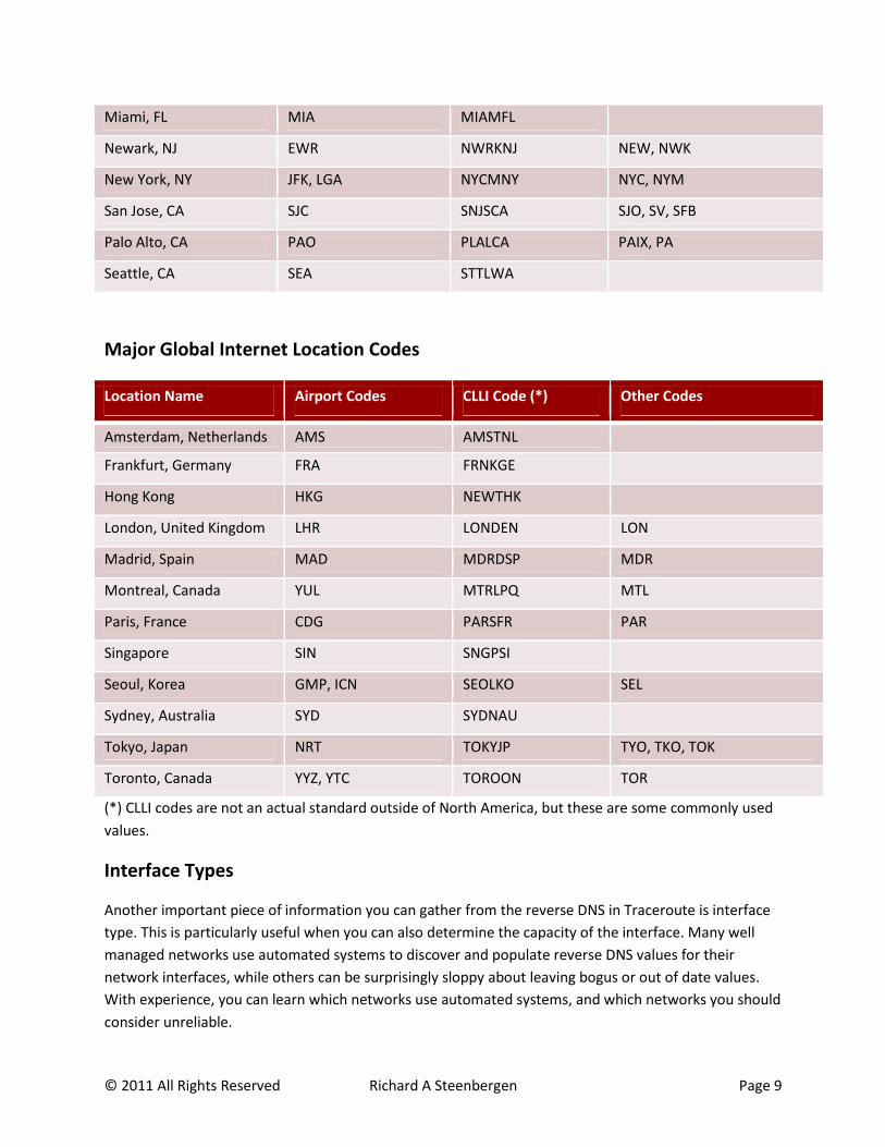
Major Global Internet Location Codes
Location Name Airport Codes CLLI Code (*) Other Codes
Amsterdam, Netherlands AMS AMSTNL
Frankfurt, Germany FRA FRNKGE
Hong Kong HKG NEWTHK
London, United Kingdom LHR LONDEN LON
Madrid, Spain MAD MDRDSP MDR
Montreal, Canada YUL MTRLPQ MTL
Paris, France CDG PARSFR PAR
Singapore SIN SNGPSI
Seoul, Korea GMP, ICN SEOLKO SEL
Sydney, Australia SYD SYDNAU
Tokyo, Japan NRT TOKYJP TYO, TKO, TOK
Toronto, Canada YYZ, YTC TOROON TOR
(*) CLLI codes are not an actual standard outside of North America, but these are some commonly used
values.
Interface Types
Another important piece of information you can gather from the reverse DNS in Traceroute is interface
type. This is particularly useful when you can also determine the capacity of the interface. Many well
managed networks use automated systems to discover and populate reverse DNS values for their
network interfaces, while others can be surprisingly sloppy about leaving bogus or out of date values.
With experience, you can learn which networks use automated systems, and which networks you should
consider unreliable.

© 2011 All Rights Reserved Richard A Steenbergen Page 10
In many circumstances, the interface numbering scheme can even help you identify the make and even
the model of the router in question. For example, consider xe-11-1-0.edge1.NewYork1.Level3.net. The
naming scheme xe-#-#-# is a Juniper 10GE port in slot 11, port 1. You immediately know that you are
dealing with a 12-slot device, and since the 10GE port is showing up as “port 1” you know that there is
more than one 10GE port per slot. This must be a Juniper MX960 router; no other router could possibly
fit this interface name profile.
The following table shows the naming schemes used by the most common types of routers:
Interface Type Cisco IOS Cisco IOS XR Juniper
Fast Ethernet Fa#/# fe-#/#/#
Gigabit Ethernet Gi#/# Gi#/#/#/# ge-#/#/#
10 Gigabit Ethernet Te#/# Te#/#/#/# xe-#/#/# (*)
SONET Pos#/# POS#/#/#/# so-#/#/#
T1 Se#/# t1-#/#/#
T3 t3-#/#/#
Ethernet Bundle Po# / Port-channel# BE#### ae#
SONET Bundle PosCh# BS#### as#
Tunnel Tu# TT# or TI# ip-#/#/# or gr-#/#/#
ATM ATM#/# AT#/#/#/# at-#/#/#
Vlan Vl### Gi#/#/#/#.### ge-#-#-#.###
(*) Some Juniper routers used interface names of “ge-“ for 10 Gigabit Ethernet interfaces on certain
early revisions of hardware.
Router Types / Roles
Identifying router types and roles can also be useful in understanding a Traceroute. For example, if you
can tell that a router is named BR1, and is most likely a border router, you may be able to quickly
identify the next hop as belonging to a different network even if there is no reverse DNS provided. The
hardest part about interpreting this data is that every network using their own naming convention, so
you need to know something about the network in question in order to make an educated guess about
their router types. Still, many networks use common themes based off of generic names and concepts,
so you at least have a reasonable shot at getting this right.

© 2011 All Rights Reserved Richard A Steenbergen Page 11
Common names for core routers include CR (Core Router), Core, GBR (Gigabit Backbone Router), BB
(Backbone), CCR, EBR (Ethernet Backbone Router), etc. Common names for peering edge routers include
BR (Border Router), Border, Edge, IR (Interconnection Router), IGR (Internet Gateway Router), Peer, etc.
Common names for customer aggregation routers include AR (Aggregation Router), Aggr, Cust, CAR
(Customer Access Router), HSA (High Speed Access), GW (Gateway), etc.
Of course, not every network following their own naming conventions, so don’t get too caught up in
identifying these roles. Some networks are better than others about following these standards, so while
one network might one day decide to terminate a customer on a border router because it is convenient,
another network might NEVER do this. Experience will help you determine which networks are likely to
fall into which category.
Network Boundaries
Identifying network boundaries (where the packet crosses from one network to another) is extremely
important to troubleshooting problems with Traceroute, because these tend to be the points at which
administrative policies change, greatly influencing the final results. For example, when crossing from
network A to network B, you may find that different local-preference values (based on administrative
policies like the price of transit from a particular provider) have completely changed the return path of
the ICMP TTL Exceed packet.
Network boundaries also tend to be points where capacity and routing policy is the most constrained
(after all, it’s usually harder to work with another network than it is to work within your own network),
and are thus more likely to be problem areas. Identifying the type of relationship between two networks
(i.e. transit provider, peer, or customer) can also be helpful in understanding where the problem is
occurring, though often more for political than technical reasons. Having knowledge about which
direction the money is flowing can help reveal which side is responsible for fixing the problem, or for not
maintaining sufficient capacity on a particular link.
Sometimes it is very easy to spot a network boundary just by looking for the DNS change. For example:
4 te1-2-10g.ar3.DCA3.gblx.net (67.17.108.146)
5 sl-st21-ash-8-0-0.sprintlink.net (144.232.18.65)
Unfortunately, it isn’t always that easy. The problem usually stems from the process of assigning the /30
(or /31) IPs used on the network boundary interface. The convention followed by most networks is that
in a provider/customer relationship the provider supplies the interface IPs, but in a relationship between
peers there may be no clear answer as to which side should provide the /30, or they may simply take
turns. The network who supplies the /30 for the interface maintains control over the DNS for the entire
block, which usually means that the only way for the other party to request a particular DNS value is to
send an e-mail and ask for it. This often leads to DNS values such as:
4 po2-20G.ar5.DCA3.gblx.net (67.16.133.90)
5 cogent-1.ar5.DCA3.gblx.net (64.212.107.90)

© 2011 All Rights Reserved Richard A Steenbergen Page 12
In the above example, hop 5 is actually terminated on Cogent’s router, but the /30 between these two
networks is being provided by gblx.net. You can further confirm this by looking at the other side of the
/30, i.e. the egress interface that you can’t see in Traceroute.
> host 64.212.107.89
89.107.212.64.in-addr.arpa domain name pointer te2-3-10GE.ar5.DCA3.gblx.net.
The multiple references to the ar5.DCA3 router is a clear indicator that hop 5 is NOT a Global Crossing
router, even with the “cogent” hint in DNS. In this particular instance, the interface IPs between these
two networks is 64.212.107.88/30, where 64.212.107.89 is the Global Crossing side, and 64.212.107.90
is the Cogent side.
Sometimes there will be no useful DNS data at all, for example:
2 po2-20G.ar4.DCA3.gblx.net (67.16.133.82)
3 192.205.34.109 (192.205.34.109)
4 cr2.wswdc.ip.att.net (12.122.84.46)
In the above Traceroute, is the border between Global Crossing and AT&T router at hop 3, or hop 4?
One way you may be able to identify the boundary is to look at the owner of the IP block. In the example
above, the “whois” tool shows that the 192.205.34.109 IP is owned by AT&T. Using this information, you
know that hop 3 is the border between these two networks, and AT&T is the one supplying the /30.
Being able to identify network boundaries is critical for troubleshooting, so you know which network to
contact when there is a problem. For example, imagine you saw the following Traceroute:
4 po2-20G.ar5.DCA3.gblx.net (67.16.133.90)
5 cogent-1.ar5.DCA3.gblx.net (64.212.107.90)
6 * * *
7 * * *
etc, etc, the packet never reaches the destination following this point
Who would you contact about this issue, Global Crossing or Cogent? If you couldn’t identify the network
boundary, you might naively assume that you should be contacting Global Crossing about the issue,
since gblx.net is the last thing that shows up in the Traceroute. Unfortunately, they wouldn’t be able to
help you, all they would be able to say is “we’re successfully handing the packet off to Cogent, you’ll
have to talk to them to troubleshoot this further”. Being able to identify the network boundary greatly
reduces the amount of time it takes to troubleshoot an issue, and the number of unnecessary tickets
you will need to open with another network’s NOC.
Some networks will try to make it obvious where their customer demark is, with clear naming schemes
like networkname.customer.alter.net. Other networks are a little more subtle about it, sometimes
referencing the ASN or name of the peer. These are almost always indicators of a network boundary,
which should help steer your troubleshooting efforts.

© 2011 All Rights Reserved Richard A Steenbergen Page 13
Prioritization and Rate Limiting
The latency values reported by Traceroute are based on the following 3 components:
1. The time taken for the probe packet to reach a specific router, plus
2. The time taken for that router to generate an ICMP TTL Exceed packet, plus
3. The time taken for the ICMP TTL Exceed packet to return to the Traceroute source.
Items #1 and #3 are based on actual network conditions which affect all forwarded traffic in the same
way, but item #2 is not. Any delay caused by the router generating the ICMP TTL Exceed packet will
show up in a Traceroute as an increase in latency, or even a completely dropped packet.
To understand how routers handle Traceroute packets, you need to understand the basic architecture of
a modern router. Even state-of-the-art hardware based routers capable of handling terabits of traffic do
not handle every function in hardware. All routers have some software components to handle complex
or unusual “exception packets”, and the ICMP generation needed by Traceroute falls into this category.
Data Plane – Packets forwarded through the router.
o Fast Path – Hardware based forwarding of ordinary packets.
Examples: Almost every packet in normal Internet traffic.
o Slow Path – Software based handling of “exception packets”.
Examples: IP Options, ICMP Generation, etc.
Control Plane – Packets forwarded to the router.
o Examples: BGP, IGP, SNMP, CLI (telnet/ssh), ping, or any other packet sent
directly to a local IP address on the router.
Depending on the design of the router, the “Slow Path” of ICMP generation may be handled by
a dedicated CPU (on larger routers these are often distributed onto each line-card), or it may
share the same CPU as the Control Plane. Either way, ICMP generation is considered to be one
of the lowest priority functions of the router, and is typically rate-limited to very low values
(typically in the 50-300 packets/sec range, depending on the device).
When ICMP generation occurs on the same CPU as the Control Plane, you may notice that
events like BGP churn or even heavy CLI use (such as running a computationally intensive
“show” command) will noticeably delay the ICMP generation process. One of the biggest
examples of this type of behavior is the Cisco “BGP Scanner” process, which runs every 60
seconds to perform internal BGP maintenance functions on most IOS based devices. On a
router without a dedicated “Data Plane - Slow Path” CPU (such as on the popular Cisco 6500
and 7600-series platforms), Traceroute users will notice latency spikes on the device every 60
seconds as this scanner runs.

© 2011 All Rights Reserved Richard A Steenbergen Page 14
It is important to note that this type of latency spike is cosmetic, and only affects Traceroute (by
delaying the returning ICMP TTL Exceed packet). Traffic forwarded through the router via the
normal “Fast Path” method will be unaffected. An easy way to detect these cosmetic spikes is
to look at the future hops in the Traceroute. If there was a real issue causing increased latency
or packet loss on all traffic forwarded through the interface, then by definition you would see
the cumulative effects in all future Traceroute hops. If you see a latency spike on one
Traceroute hop, and it goes away in the next hop, you can easily deduce that the spike was
actually caused by a cosmetic delay in the ICMP generation process.
In the following example, you can see a cosmetic latency spike which is not a real issue. Note
that the increased latency does not continue into future hops.
1 xe-4-1-0.cr2.ord1.us.nlayer.net (69.22.142.32) 18.957 ms 18.950 ms 18.991 ms
2 ae3-40g.cr1.ord1.us.nlayer.net (69.31.111.153) 19.056 ms 19.008 ms 19.129 ms
3 te7-1.ar1.slc1.us.nlayer.net (69.22.142.102) 54.105 ms 90.090 ms 54.285 ms
4 xe-2-0-1.cr1.sfo1.us.nlayer.net (69.22.142.97) 69.403 ms 68.873 ms 68.885 ms
Asymmetric Routing
One of the most basic concepts of routing on the Internet is that there is absolutely no guarantee of
symmetrical routing of traffic flowing between the same end-points but in opposite directions. Regular
IP forwarding is done by destination-based routing lookups, and each router can potentially have its own
idea about where traffic should be forwarded.
As we discussed earlier, Traceroute is only capable of showing you the forward path between the source
and destination you are trying to probe, even though latency incurred on the reverse path of the ICMP
TTL Exceed packets is part of the round-trip time calculation process. This means that you must also
examine the reverse path Traceroute before you can be certain that a particular link is responsible for
any latency values you observe in a forward Traceroute.
Asymmetric paths most often start at network boundaries, because this is where administrative policies
are most likely to change. For example, consider the following Traceroute:
3 te1-1.ar2.DCA3.gblx.net (69.31.31.209) 0.719 ms 0.560 ms 0.428 ms
4 te1-2-10g.ar3.DCA3.gblx.net (67.17.108.146) 0.574 ms 0.557 ms 0.576 ms
5 sl-st21-ash-8-0-0.sprintlink.net (144.232.18.65) 100.280 ms 100.265 ms 100.282 ms
6 144.232.20.149 (144.232.20.149) 102.037 ms 101.876 ms 101.892 ms
7 sl-bb20-dc-15-0-0.sprintlink.net (144.232.15.0) 101.888 ms 101.876 ms 101.890 ms
This Traceroute shows a 100ms increase in latency between Global Crossing in Ashburn VA and Sprint in
Ashburn VA, and you’re trying to figure out why. Obviously distance isn’t the cause for the increased

© 2011 All Rights Reserved Richard A Steenbergen Page 15
latency, since these devices are both in the same city. It could be congestion between Global Crossing
and Sprint, but this isn’t guaranteed. After the packets cross the boundary between Global Crossing and
Sprint, the administrative policy is also likely to change. In this specific example, the reverse path from
Sprint to the original Traceroute source travels via a different network, which happens to have a
congested link. Someone looking at only the forward Traceroute would never know this though, which is
why obtaining both forward and reverse Traceroutes is so important to proper troubleshooting.
But asymmetric paths don’t only start at network borders, they can potentially occur at each and every
router along the way. A common example of this is when two networks interconnect with each other in
multiple locations. Most routing between networks on the Internet uses a concept called “hot potato”,
i.e. the goal is to get the traffic off of your network and onto the other network as quickly as possible.
This means that a Traceroute which spans a large distance and goes by multiple interconnection points
can have many different return paths, even between the same two networks. Consider the following
example:
In this scenario, traffic is passing between two independent networks, one with grey routers and one
with blue routers. All of the forward path traffic is coming in via Washington DC, but the path of the
return traffic changes at each hop. At the first hop, indicated in purple, the return traffic comes back
over the same interface in Washington DC as the forward traffic. By the second hop, indicated in red,
the packet has made its way to Chicago, and the ICMP TTL Exceed return packet will now traverse the
interconnection in Chicago rather than the one in Washington DC. By the third hop, indicated in green,
the reverse path has changed again.
If there was congestion between the blue and grey networks in Chicago, a Traceroute might show the
increased latency for one hop, but by the next hop the packets would no longer be traversing this
interface. Alternatively, there could be congestion on the grey network’s backbone between San Jose
and Washington DC, which the first two probes would not encounter because they do not traverse that
path. The forward Traceroute would indicate a severe increase in latency and/or packet loss on the blue
Washington DC
Chicago IL
San Jose CA
© 2011 All Rights Reserved Richard A Steenbergen Page 16
network between Chicago and San Jose, even though the actual cause of the problem lies with the grey
network.
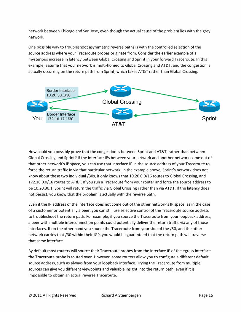
One possible way to troubleshoot asymmetric reverse paths is with the controlled selection of the
source address where your Traceroute probes originate from. Consider the earlier example of a
mysterious increase in latency between Global Crossing and Sprint in your forward Traceroute. In this
example, assume that your network is multi-homed to Global Crossing and AT&T, and the congestion is
actually occurring on the return path from Sprint, which takes AT&T rather than Global Crossing.
How could you possibly prove that the congestion is between Sprint and AT&T, rather than between
Global Crossing and Sprint? If the interface IPs between your network and another network come out of
that other network’s IP space, you can use that interface IP in the source address of your Traceroute to
force the return traffic in via that particular network. In the example above, Sprint’s network does not
know about these two individual /30s, it only knows that 10.20.0.0/16 routes to Global Crossing, and
172.16.0.0/16 routes to AT&T. If you run a Traceroute from your router and force the source address to
be 10.20.30.1, Sprint will return the traffic via Global Crossing rather than via AT&T. If the latency does
not persist, you know that the problem is actually with the reverse path.
Even if the IP address of the interface does not come out of the other network’s IP space, as in the case
of a customer or potentially a peer, you can still use selective control of the Traceroute source address
to troubleshoot the return path. For example, if you source the Traceroute from your loopback address,
a peer with multiple interconnection points could potentially deliver the return traffic via any of those
interfaces. If on the other hand you source the Traceroute from your side of the /30, and the other
network carries that /30 within their IGP, you would be guaranteed that the return path will traverse
that same interface.
By default most routers will source their Traceroute probes from the interface IP of the egress interface
the Traceroute probe is routed over. However, some routers allow you to configure a different default
source address, such as always from your loopback interface. Trying the Traceroute from multiple
sources can give you different viewpoints and valuable insight into the return path, even if it is
impossible to obtain an actual reverse Traceroute.
You
Global Crossing
AT&T Sprint
Border Interface 10.20.30.1/30
Border Interface 172.16.17.1/30

© 2011 All Rights Reserved Richard A Steenbergen Page 17
Load Balancing Across Multiple Paths
Within a complex IP network, there is often a need to load balance traffic across multiple physical links
between a particular source and destination. There are two primary ways to accomplish this, a layer-2
based Link Aggregation protocol (often called a LAG, such as 802.3ad), and layer-3 based Equal Cost
Multi-Path (ECMP) routing. Layer 2 based LAGs are invisible to Traceroute, but layer-3 based ECMP is
often detectable. When multiple paths are included in Traceroute results, it can significantly increase
the difficulty of correctly interpreting the results and diagnosing any potential problems.
In order to prevent packet reordering within a flow, which would be detrimental to many applications,
all load balancing techniques use a hash algorithm to keep individual layer 4 flows mapped onto the
same physical path. But as we discussed earlier, many Traceroute implementations send multiple probes
per hop, and the incrementing layer 4 port numbers will be interpreted by the load balancing hashing
algorithms as unique flows. This means that each Traceroute probe has the potential to travel down a
different path, depending on how the hashing algorithms are configured on each individual router.
In the simplest ECMP configuration, consider the following scenario:
An example of the kind of output you will see from this configuration is:
6 ldn-bb2-link.telia.net (80.91.251.14) 74.139 ms 74.126 ms
ldn-bb1-link.telia.net (80.91.249.77) 74.144 ms
7 hbg-bb1-link.telia.net (80.91.249.11) 89.773 ms
hbg-bb2-link.telia.net (80.91.250.150) 88.459 ms 88.456 ms
8 s-bb2-link.telia.net (80.91.249.13) 105.002 ms
s-bb2-link.telia.net (80.239.147.169) 102.647 ms 102.501 ms
Depending on the Traceroute utility the output may not be formatted quite as nicely as this, but you can
easily see the multiple routers that are being encountered at each hop count position. In the example
above, Telia is load balancing traffic between pairs of routers (bb1 and bb2) in each city.
A slightly more complex example illustrates what happens when packets are ECMP routed between two
“somewhat” parallel paths:
Router B2 Router C2
SRC Router A Router B1 Router C1 Router D
DST
© 2011 All Rights Reserved Richard A Steenbergen Page 18
4 p16-1-0-0.r21.asbnva01.us.bb.gin.ntt.net (129.250.5.21) 0.571 ms 0.604 ms 0.594 ms
5 p16-4-0-0.r00.chcgil06.us.bb.gin.ntt.net (129.250.5.102) 25.981 ms
p16-1-2-2.r21.nycmny01.us.bb.gin.ntt.net (129.250.4.26) 7.279 ms 7.260 ms
6 p16-2-0-0.r21.sttlwa01.us.bb.gin.ntt.net (129.250.2.180) 71.027 ms
p16-1-1-3.r20.sttlwa01.us.bb.gin.ntt.net (129.250.2.6) 66.730 ms 66.535 ms
In this example, NTT is load balancing traffic across the following two paths:
Ashburn VA – New York NY – Seattle WA
Ashburn VA – Chicago IL – Seattle WA
This is a perfectly valid configuration, the flow hashing algorithm protects against any packet reordering,
but the resulting Traceroute output is potentially confusing. Someone who didn’t understand what was
happening here might think that the packet was traveling from Ashburn to Chicago to New York to
Seattle, routing “backwards” from the normal path it should be following.
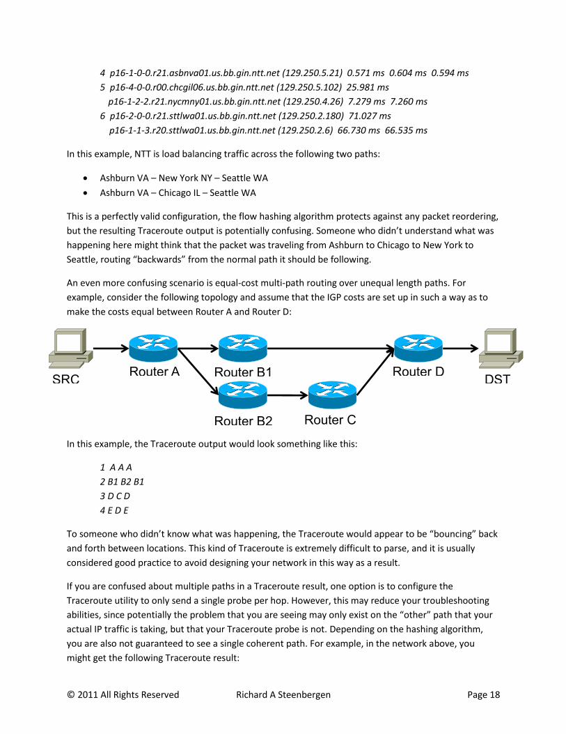
An even more confusing scenario is equal-cost multi-path routing over unequal length paths. For
example, consider the following topology and assume that the IGP costs are set up in such a way as to
make the costs equal between Router A and Router D:
In this example, the Traceroute output would look something like this:
1 A A A
2 B1 B2 B1
3 D C D
4 E D E
To someone who didn’t know what was happening, the Traceroute would appear to be “bouncing” back
and forth between locations. This kind of Traceroute is extremely difficult to parse, and it is usually
considered good practice to avoid designing your network in this way as a result.
If you are confused about multiple paths in a Traceroute result, one option is to configure the
Traceroute utility to only send a single probe per hop. However, this may reduce your troubleshooting
abilities, since potentially the problem that you are seeing may only exist on the “other” path that your
actual IP traffic is taking, but that your Traceroute probe is not. Depending on the hashing algorithm,
you are also not guaranteed to see a single coherent path. For example, in the network above, you
might get the following Traceroute result:
Router B2 Router C
SRC Router A Router B1 Router D
DST

© 2011 All Rights Reserved Richard A Steenbergen Page 19
1 A
2 B1
3 C
4 DST
It is also possible that the routers your Traceroute probes are traveling through are configured to
perform flow hashing based on only the layer 3 fields of the packet, and not to use any of the layer 4
fields. When this happens, the path that your traffic takes through the network depends on the specific
combination of source and destination IP addresses, and Traceroute probes may not be able to see the
other possible paths simply by incrementing the layer 4 port values. If you see connectivity issues
between a particular source and destination pair, but are unable to perform a Traceroute between
those exact same IPs, one possible technique to locate the other paths is simply to manually increment
the destination IP address by 1. For example, if you are performing a Traceroute to 172.16.2.3 try also
performing a Traceroute to 172.16.2.4 and 172.16.2.5 to see if the path in the middle changes.
MPLS and Traceroute
When networks use Multi-Protocol Label Switching (MPLS) to carry IP traffic across their backbone, it
can have several effects on Traceroute results.
Disabling TTL Decrement
One feature of MPLS is the ability to hide router hops inside of a label switched path (LSP), by disabling
the decrementing of the TTL value on label switching routers (LSRs). Because an LSP acts as a virtual
layer 2 path, and has its own TTL value on the MPLS label, there is no need to decrement the IP packet
TTL at every router along the way. Some networks choose to configure this behavior in order to hide
portions of their topology, for a wide variety of technical or business reasons.
ICMP Tunneling
Some very large networks choose to operate an MPLS-only core infrastructure, using routers which
don’t carry an actual IP routing table. This is perfectly fine for most traffic in the core, which is already
encapsulated inside MPLS and thus doesn’t ever need to do an IP routing lookup, but it presents a
problem for Traceroute; How can a router in the middle of a Traceroute return an ICMP TTL Exceed
message if it can’t do a routing lookup to deliver the ICMP message?
One solution to this problem is a technique called ICMP Tunneling. When doing ICMP Tunneling, if a
MPLS label-switching router (LSR) is forced to drop a packet and generate an ICMP response while the
packet is inside of an LSP, it will insert the ICMP message back into the same LSP as the original packet.
This has the effect of forcing the ICMP message to travel all the way to the original destination of the
probe packet, rather than immediately returning to the sender. The message will eventually get there,
but it makes the latency reported in Traceroute appear to all be the same value as the final destination
for every hop inside of the LSP.
© 2011 All Rights Reserved Richard A Steenbergen Page 20
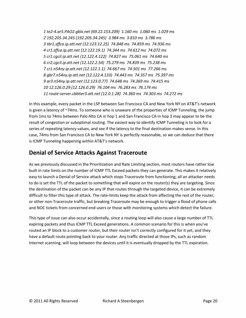
1 te2-4.ar5.PAO2.gblx.net (69.22.153.209) 1.160 ms 1.060 ms 1.029 ms
2 192.205.34.245 (192.205.34.245) 3.984 ms 3.810 ms 3.786 ms
3 tbr1.sffca.ip.att.net (12.123.12.25) 74.848 ms 74.859 ms 74.936 ms
4 cr1.sffca.ip.att.net (12.122.19.1) 74.344 ms 74.612 ms 74.072 ms
5 cr1.cgcil.ip.att.net (12.122.4.122) 74.827 ms 75.061 ms 74.640 ms
6 cr2.cgcil.ip.att.net (12.122.2.54) 75.279 ms 74.839 ms 75.238 ms
7 cr1.n54ny.ip.att.net (12.122.1.1) 74.667 ms 74.501 ms 77.266 ms
8 gbr7.n54ny.ip.att.net (12.122.4.133) 74.443 ms 74.357 ms 75.397 ms
9 ar3.n54ny.ip.att.net (12.123.0.77) 74.648 ms 74.369 ms 74.415 ms
10 12.126.0.29 (12.126.0.29) 76.104 ms 76.283 ms 76.174 ms
11 route-server.cbbtier3.att.net (12.0.1.28) 74.360 ms 74.303 ms 74.272 ms
In this example, every packet in the LSP between San Francisco CA and New York NY on AT&T’s network
is given a latency of ~74ms. To someone who is unaware of the properties of ICMP Tunneling, the jump
from 1ms to 74ms between Palo Alto CA in hop 1 and San Francisco CA in hop 3 may appear to be the
result of congestion or suboptimal routing. The easiest way to identify ICMP Tunneling is to look for a
series of repeating latency values, and see if the latency to the final destination makes sense. In this
case, 74ms from San Francisco CA to New York NY is perfectly reasonable, so we can deduce that there
is ICMP Tunneling happening within AT&T’s network.
Denial of Service Attacks Against Traceroute
As we previously discussed in the Prioritization and Rate Limiting section, most routers have rather low
built in rate limits on the number of ICMP TTL Exceed packets they can generate. This makes it relatively
easy to launch a Denial of Service attack which stops Traceroute from functioning; all an attacker needs
to do is set the TTL of the packet to something that will expire on the router(s) they are targeting. Since
the destination of the packet can be any IP that routes through the targeted device, it can be extremely
difficult to filter this type of attack. The rate-limits keep the attack from affecting the rest of the router,
or other non-Traceroute traffic, but breaking Traceroute may be enough to trigger a flood of phone calls
and NOC tickets from concerned end-users or those with monitoring systems which detect the failure.
This type of issue can also occur accidentally, since a routing loop will also cause a large number of TTL
expiring packets and thus ICMP TTL Exceed generations. A common scenario for this is when you’ve
routed an IP block to a customer router, but their router isn’t correctly configured for it yet, and they
have a default route pointing back to your router. Any traffic directed at those IPs, such as random
Internet scanning, will loop between the devices until it is eventually dropped by the TTL expiration.