Computer Vision November 2003 L1.1© 2003 by Davi Geiger

Tracking

We are given a contour with coordinates ={x1 , x2 , … , xN} at the initial frame were the image is IWe are interested in tracking this contour through several image frames, say through T image frames given by

We will denote each of these contours by t and so 1 = t=1 . We will track each of the coordinates of the initial contour, i.e., we will focus on the tracking of the N initial coordinates. Thus, at any time the new contour will be characterized by t = {x1 , x2 , … , xN }, and these coordinates need not be connected. In order to create a connected contour at each frame one may fit a spline or another form of linking of this sequence of N coordinates. In a Bayesian framework we attempt to obtain the probability

)1()|( 11 Ip

11,...,, IIII TTT

We can make measurements at each image frame, accumulate them over time denoting by and we ask “Which state (coordinates) the contour will be at that time given all the measurements ?”

1I

Computer Vision November 2003 L1.2© 2003 by Davi Geiger

Propagating Probability Density

)2()|(),|()|(

),|(

)|,()|(

),|(

)|()|(

),|(

)|(),|()|(

1

),|()|(

11

11

11

11

11

11

1111

1111

dIPIpIIp

IIp

dIpIIp

IIp

IpIIp

IIp

IpIIpIIp

IIPIP

An interesting expansion of (1) is given by:

Assuming that such probabilities can be obtained, namely

than we have a recursive method to estimate,)|(),,|(),,|( 1111 IIpIpIIp

)|( 11 IP

PredictCorrect or make

Measurements)|(),|()|,( CBPCBAPCBAP

)|(),|()|(

1),|( :)on al(condition sBaye' CAPCABP

CBPCBAPC

B

CBAPCAP )|,()|( :yProbabilit Marginal

Computer Vision November 2003 L1.3© 2003 by Davi Geiger

Assumptions

Independence assumption on data generation, i.e., the current state completely defines the probability of the measurements/data (often the previous data is also neglected)

First order Markov process, i.e., the current state of the system is completely described by the immediate previous state, and possibly the data (often the data is also neglected).

)|( 1 IIp

)|(

),|(

1

1

p

or

Ip

)|(

),|(

11

11

Ip

or

IIp

This is a normalization constant that can always be computed by normalizing the recurrence equation (2)

Computer Vision November 2003 L1.4© 2003 by Davi Geiger

Linear Dynamics

);()|(

);()|( 111

m

d

MNIp

DNp

matrices.linear are and .matrix covariance and r mean vectowith

Gaussian a i.e., ,on distributi normal blemultivaria theis );(where

DM

N

Examples

Random Walk

Points moving with constant velocity

Points moving with constant acceleration

Periodic motion

Computer Vision November 2003 L1.5© 2003 by Davi Geiger

noise todue ismotion all

10

01);()|( 1111

DxDNxxpy

xx dx

Drift: New position is the previous one plus noise d

Random Walk of a Point

Computer Vision November 2003 L1.6© 2003 by Davi Geiger

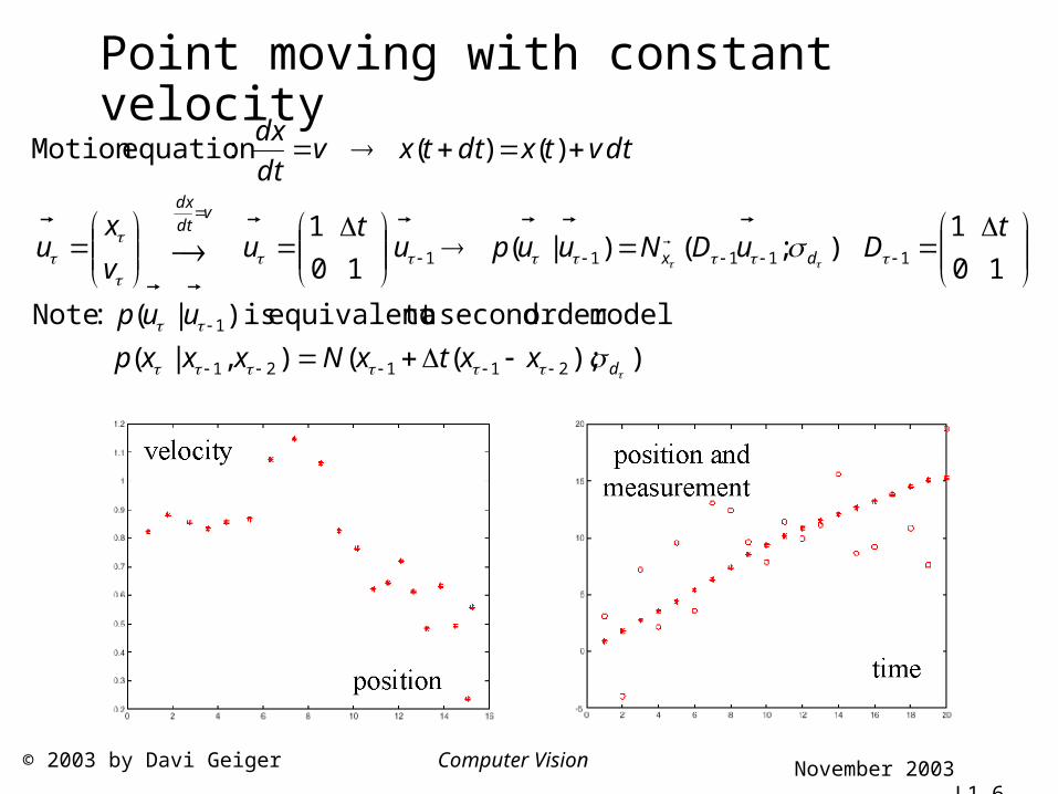
Point moving with constant velocity

));((),|(

modelorder second a toequivalent is)|( :Note

10

1);()|(

10

1

)()( :equationMotion

21121

1

11111

d

dx

vdt

dx

xxtxNxxxp

uup

tDuDNuupu

tu

v

xu

dtvtxdttxvdt

dx

Computer Vision November 2003 L1.7© 2003 by Davi Geiger

Point moving with constant acceleration

d

du

xxxtxxtxNxxxxp

dtadttvtxtxuup

t

t

DuDNuup

a

v

x

u

dtatvdttv

);2()(2

1)(),,|(

,)(2

1)()()(using model,order thirda toequivalent is)|(:Note

100

10

01

);()|(

)()( :onacceleraticonstant h Motion wit

2312

211321

21

1111

Computer Vision November 2003 L1.8© 2003 by Davi Geiger

Point moving with periodic motion

0

0);()|(

)()()()(

)()()()( equations coupledorder first toequivalent

cos)(solution periodic)( :Motion Periodic

1111

2

2

t

tDuDNuup

v

xu

dttxtvdttvtxdt

dv

dttvtxdttxtvdt

dx

tAtxtxdt

xd

du

Computer Vision November 2003 L1.9© 2003 by Davi Geiger

111111

1 )|(),|()|(

),|()|(

1

dxIxPIxxpIIp

IxIpIxP

x

Tracking one point (dynamic programming like)

Equation (2) is written as

t

)|( 11 xIP

)|( 1 xxp

xx

x

IxFIIpIxF

IxFIxP

IxPIxxpIxIpIxF

)|()|(: thatnote)|(

)|()|(

)|(),|(),|()|(

1

11111

1

)|( xIp

x1x

)|( IxP

)|( 11 IxP

Computer Vision November 2003 L1.10© 2003 by Davi Geiger

Kalman Filter (Special Case of a Linear System)Simplify calculation of the probabilities due to good Gaussian properties (applied to ) ),|(and),|( 111 IpIIp

)|( IP

111111

1 )|(),|()|(

),|()|(

1

dIPIpIIp

IIpIP

Reminder: From equation (2) we have

1D case: For one dimension point and Gaussian distributions

11111

)|();()|(

);()|(

1

dxyxPxdNyyp

xmNyxP

x

dxmy

Kalman observed the recurrence: if

then

where

);()|( 1111 1

x

NyxP

21

222

2

)(,)()(

)(

ddm

m22

21

2

)(

)(and

m

m

m

dym

);()|( x

NyxP

Computer Vision November 2003 L1.11© 2003 by Davi Geiger

Then

21

21

11'

21

2111'

1'

11111

111

)()(;);(

)(

)()(;);(

)(,

);();();(

)(

);();();()|(

1

1

1

1

1

1

ddNmymNc

i

ddxdNxmNc

iidcc

dxNdxdNxmNdc

i

dxNxdNxmNcyxP

dxmx

dmy

x

x

dxmy

x

x

dxmy

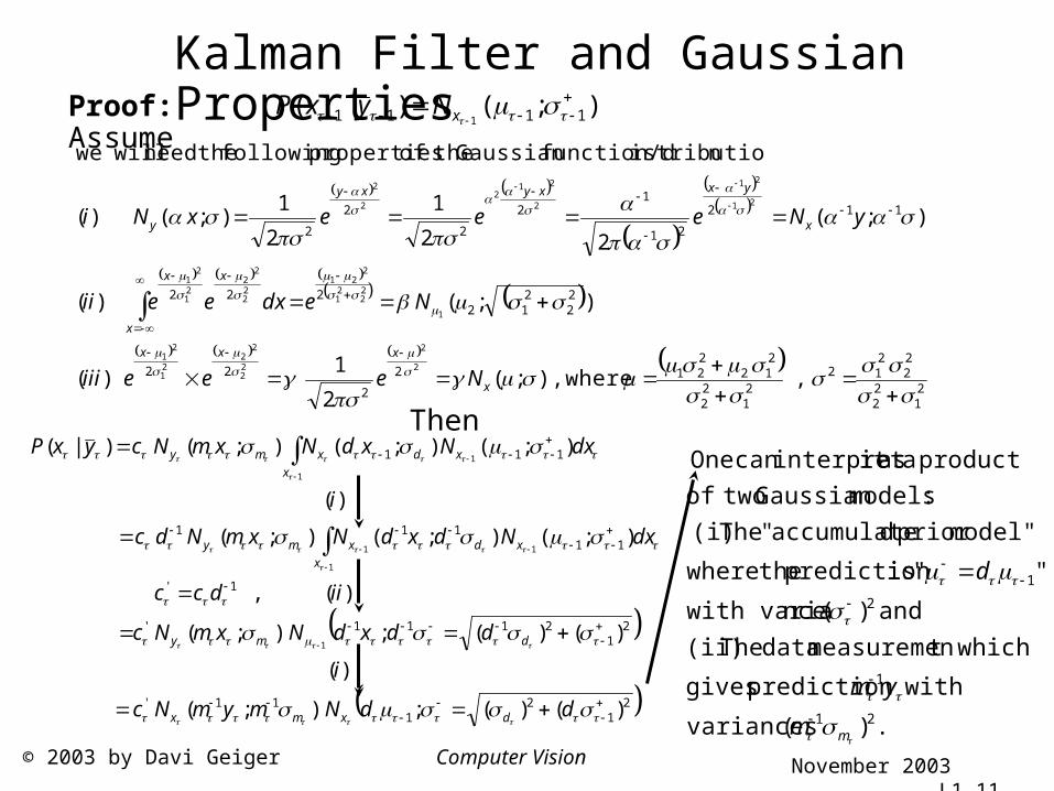
Kalman Filter and Gaussian PropertiesProof: Assume );()|( 1111 1

x

NyxP

21

22

22

212

21

22

212

2212

2

22

22

212

222

112

21

12

2

2

2

, where),;(2

1)(

);()(

);(22

1

2

1);()(

nistributiofunction/dGaussian theof properties following theneed willwe

2

2

22

22

21

21

1

22

21

221

22

22

21

21

21

21

2

212

2

2

x

xxx

x

-x

x

x

yxxyxy

y

Neeeiii

Nedxeeii

yNeeexNi

.)( variances

with prediction gives

t which measuremen data The (ii)

and)( ncewith varia

"" is prediction thewhere

model"prior daccumulate" The (i)

:modelsGaussian twoof

product a asit interpret can One

21

1

2

1

mm

ym

d

Computer Vision November 2003 L1.12© 2003 by Davi Geiger

Kalman Filter …(continuing the proof)

;

)(

)(;

)(

)(

)()(

)()(;

)()(

)()(

)(

)()(;);(

...)|(

22

22

22

21

2

212

221

212

211

21'

21

21

11'

x

m

m

m

mx

m

m

m

mx

dxmx

N

mm

dymN

m

m

m

mdymNc

iii

ddNmymNc

yxP

Computer Vision November 2003 L1.13© 2003 by Davi Geiger

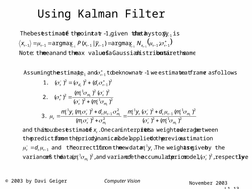
Using Kalman Filter

ly.respective ,)(,modelprior daccumulate theof varianceand ,)( data, theof variances

by thegiven are weightsThe. data new thefrom "correction" theand

estimationpreviou the toapplied model dynamical (prior) thefrom prediction the

between average weighteda asit interpret can One. of estimatebest our is that and

)()(

)()(

)(

)(.3

)()(

)()()(.2

)()()(.1

follows as frameat estimate we 1-at known be to and estimate theAssuming

221

11

212

211

21

22

21

21

212

2212

21

22

11

m

m

m

m

m

m

m

d

m

ymd

x

m

mdym

m

dmym

m

m

d

τx

same theare onsdistributiGaussian a of max values theandmean the:Note

; argmax)|( argmax

is hystory data given the,1-atpoint theof estimatebest The

111111

1

111

xxx NyxPx

yx

Computer Vision November 2003 L1.14© 2003 by Davi Geiger

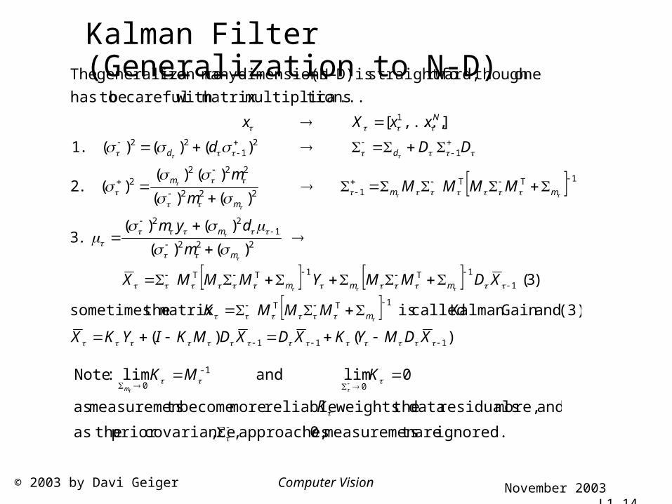
Kalman Filter (Generalization to N-D)

)()(

(3)andGain Kalman called is matrix thesometimes

)3(

)()(

)()(.3

)()(

)()()(.2

)()()(.1

],...,[

... tionsmultiplicamatrix with careful be tohas

one though rward,straightfo is D)-(N dimensionsmany tion togeneraliza The

111

1TT

1

1T1TT

222

122

1TT1222

2222

12

122

1

XDMYKXDXDMKIYKX

MMMK

XDMMYMMMX

m

dym

MMMMm

m

DDd

xxXx

m

mmm

m

m

mmm

m

dd

N

ignored. are tsmeasuremen 0, approaches, ,covarianceprior theas

and more, residuals data theweights reliable more become tsmeasuremen as

0lim andlim :Note0

-1

0

K

KMKm