Tracking aircraft with PARSAX

Master of Science Thesis

For the degree of Master of Science in

Microwave Sensing, Signals and Systems (MS3)

at the Department of Telecommunications

at Delft University of Technology

Jacco Schreuders 9749278

July 7, 2014

Faculty of Electrical Engineering, Mathematics, and Computer Science

Delft University of Technology

Delft, the Netherlands

Preface

During the period 2007-2011, the Microwave Sensing, Signals and Systems (MS3) division of TU

Delft developed PARSAX, a high resolution FMCW research radar. Since it moves relatively slow,

and it cannot utilize techniques such as monopulse or conical scanning, it is unable to track aircraft

by itself. An external source of information is needed, which is provided by ADS-B, a technique

which allows aircraft to broadcast their own position and velocity at regular intervals. This thesis

presents the development of a tracking algorithm which can be used to automatically track aircraft

with PARSAX by using the information sent via ADS-B.

I would like to thank my supervisor Dr. Krasnov for his advice and encouragement. Also thanks to

Prof. Yarovoy for the interesting assignment and for his advice about presentations. I would also

like to thank Etiënne Goossens for his help with programming, and lastly, thanks to Dr. Janssen for

keeping tabs on things.

The thesis committee members are:

Prof. dr. A. Yarovoy, Microwave Sensing, Signals and Systems (MS3), TU Delft

Dr. O. Krasnov, Microwave Sensing, Signals and Systems (MS3), TU Delft

Dr. ir. G.J.M. Janssen, Wireless and Mobile Communications (WMC), TU Delft

Ir. R. Harmanny, Thales, Delft

i

Contents

Preface …............................................................................................................ i

List of figures ................................................................................................... iv

Chapter 1

Introduction …................................................................................................... 1

Chapter 2

Literature survey …............................................................................................ 3

Chapter 3

Analysis ............................................................................................................. 8

3.1 PARSAX .................................................................................................... 9

3.1.1 Characteristics of PARSAX ................................................................. 9

3.1.2 Movement of PARSAX ...................................................................... 9

3.2 ADS-B explained ....................................................................................... 12

3.3 Earth model of GPS …............................................................................... 15

3.4 Calculation of the target position relative to the radar ….................................. 18

3.4.1 Calculation of azimuth and elevation ….............................................. 19

3.4.2 Calculation of aircraft altitude …........................................................ 22

3.4.3 Calculation of the slant range …......................................................... 25

3.5 Extrapolation of the aircraft position …......................................................... 25

3.6 Simulations ….......................................................................................... 28

ii

3.6.1 Relative angular velocities of aircraft ….............................................. 29

3.6.2 Simulations of tracking aircraft with PARSAX …................................. 34

3.7 Tracking aircraft ........................................................................................ 44

3.7.1 Target model …............................................................................... 44

3.7.2 Measurement model …..................................................................... 45

3.7.3 Kalman filter …............................................................................... 45

3.7.4 Tracking algorithm …....................................................................... 46

3.8 Summary ….............................................................................................. 47

Chapter 4

Implementation …............................................................................................ 48

4.1 Hardware interfaces …............................................................................... 48

4.2 Three phases …......................................................................................... 49

4.3 Implementation of tracking time estimation …............................................... 51

4.3.1 Calculating the in-range interval ….................................................... 51

4.3.2 Calculating the interception intervals ….............................................. 52

4.3.3 Calculating simulated tracking times …............................................... 52

4.4 Implementation of the Kalman filter …......................................................... 52

4.5 Weather information …............................................................................... 53

Chapter 5

Conclusion …................................................................................................... 54

List of Acronyms ….......................................................................................... 55

Bibliography …................................................................................................ 56

iii

List of figures

3.1. The axes of rotation of PARSAX ….................................................................... 9

3.2. Elevation as a function of inclination …............................................................. 11

3.3. Azimuth offset as a function of inclination …..................................................... 11

3.4. The Kinetic SBS-3 ADS-B receiver ….............................................................. 13

3.5. Ellipsoidal model of Earth (cross-section normal to equatorial plane) …................. 15

3.6. Distances between ground level, geoid, and ellipsoid …....................................... 16

3.7. Calculation of azimuth (left) and elevation (right) …........................................... 17

3.8. ECEF and ENU coordinate systems ….............................................................. 18

3.9. The length of the normal N …......................................................................... 19

3.10. Pressure altitude versus true altitude …............................................................ 22

3.11. Required altitude accuracy as a function of range and elevation …....................... 23

3.12. Difference between geocentric and geodetic latitude …...................................... 26

3.13. Comparison between extrapolated and real trajectories …................................... 27

3.14. Differences between extrapolated and ADS-B values …..................................... 28

3.15. Angular velocities in azimuth for h = 1000 m and v = 300 kts ….......................... 29

3.16. Angular velocities in azimuth for h = 5000 m and v = 300 kts ….......................... 30

3.17. Angular velocities in azimuth for h = 10000 m and v = 300 kts …........................ 31

3.18. Angular velocities in elevation for h = 1000 m and v = 300 kts …........................ 32

3.19. Angular velocities in elevation for h = 5000 m and v = 300 kts …........................ 33

3.20. Angular velocities in elevation for h = 10000 m and v = 400 kts …...................... 34

3.21. Simulation plots of tracking a target with h = 1000, v = 300, yENU = 0, and good offset …...................................................................................................... 36

3.22. Simulation plots of tracking a target with h = 1000, v = 300, yENU = 0, and bad offset .......................................................................................................... 37

3.23. Simulation plots of tracking a target with h = 1000, v = 300, yENU = 2000, and good offset .................................................................................................. 38

iv

3.24. Simulation plots of tracking a target with h = 1000, v = 300, yENU = 2000, and bad offset .................................................................................................... 39

3.25. Simulation plots of tracking a target with h = 1000, v = 300, yENU = 3000, and good offset .................................................................................................. 40

3.26. Tracking targets with θ = 90º, h = 1000 m, v = 300 kts, and good offset …............ 41

3.27. Tracking targets with θ = 90º, h = 1000 m, v = 300 kts, and bad offset ….............. 42

3.28. Tracking simulation for combinations of altitude, speed, and azimuth offset …...... 43

4.1. System architecture ........................................................................................ 49

4.2. Tracking in progress ....................................................................................... 50

v

To my mother

Chapter 1

Introduction

During 2007-2011, the Microwave Sensing, Signals and Systems (MS3) division of TU Delft

developed the Polarimetric Agile Radar in S- And X-band (PARSAX) [1]. It is a unique, high-

resolution FMCW radar which can measure the full polarisation scattering matrix of a radar target

in one sweep by using dual orthogonal signals. It can be used in many applications, such as real-

time atmospheric and ground remote sensing, aerial and ground traffic monitoring, and as a test-bed

for the development and validation of advanced radar signals and processing algorithms.

PARSAX has not been designed to automatically track moving targets by using techniques

such as monopulse channels or fast antenna beam steering. Instead, an Automatic Dependent

Surveillance Broadcast (ADS-B) receiver can be used to decode the navigational messages which

aircraft periodically transmit. This information can be used to dynamically position the radar to

extend the observation time for fast moving targets. With this approach, data can be collected to

study airborne targets and related atmospheric phenomena such as wake vortexes. A feasibility

study and initial software development has been performed in a previous BSc project [2].

The goal of this study is to integrate the ADS-B receiver into the PARSAX radar system and

to provide the capability for stable and reliable tracking of airborne targets and related atmospheric

phenomena, during at least a few tens of seconds.

The outline of the thesis is as follows. Chapter 2 presents the results of a literature survey on

using ADS-B as an information source for tracking aircraft. Several research groups have been

trying to use ADS-B as an extra source of information to assist in aircraft tracking in the

conventional way. Since PARSAX is not a conventional tracking radar, a different approach is

needed to solve the problem. Chapter 3 describes the analysis of the problem, the limitations of

1

PARSAX, and characteristics of ADS-B. As the position of aircraft in ADS-B messages is supplied

by an on-board GPS receiver, the coordinates need to be transformed to local coordinates in order to

carry out any calculations. This transformation and a way to extrapolate the position of aircraft

allows for a simulation of the target's movement in a radar-centred spherical coordinate system, to

estimate components of its relative angular velocities, and to analyze the ability of the PARSAX

radar antenna's steering system to follow that specific target. Finally, a tracking algorithm is

developed. The implementation of this algorithm is described in Chapter 4. The conclusion and

recommendations can be found in Chapter 5.

2

Chapter 2

Literature survey

To get an idea of how to approach the problem, a literature study was performed. The results are

presented in this chapter.

For an optical communication system, a static ground station needs to be able to track a moving

receiver, and point the transmitter's telescope in its direction [3]. Important parameters are the

positions of the transmitter and receiver, and their uncertainties. The pointing resolution, which is

the smallest pointing change the transmitter can make, depends on the mechanics of the transmitter.

The update rate of the receiver's position information needs to be high enough for the transmitter to

react in time, especially in case when the receiver moves with high velocity or when the receiver is

nearby. Both these cases can be characterized by high angular velocities of the receiver relative to

the transmitter. Transmission delays and calculation times should be low enough to be negligible.

For the position determination, a GPS receiver can be used because it provides geographic positions

with good accuracy and availability. For testing purposes, the ground station consisted of a camera,

mimicking the optical transmitter, a GPS-aided inertial navigation system and an ADS-B receiver.

The receivers were represented by aircraft flying overhead with ADS-B transmitting capability.

Position information from the inertial navigation system and ADS-B messages were fed into a

tracking computer, which drove the transmitter to the correct attitudes. The maximum ADS-B

message rate is 2 Hz, which in reality will be lower since some messages will be corrupted. Bad

messages need to be filtered out before they are used and future positions of the target need to be

estimated in order to make tracking with ADS-B a success. Position and velocity predictions were

made with a g-h filter, which is a simplified version of a Kalman filter [20], where the velocity was

considered constant. This assumption is reasonable for small accelerations of the target or when

3

ADS-B updates are frequent enough. ADS-B messages were considered corrupted when the

predicted position differed by more than 1 km from the measured position.

In air traffic management (ATM), ADS-B could make a welcome additional sensor to the

standard radar trackers [4]. Increased positional accuracy would result in higher safety, efficiency

and capacity of the airspace. Accurate measurements and modelling of aircraft movements are vital

for tracking. A Kalman filter is used because it can accommodate multiple sensors and it has low

computational cost. Aircraft are modelled as points in space and their accelerations are considered

as white noise. Despite the fact that aircraft models are non-linear and that noise in reality is not

Gaussian and white, the Kalman filter has been used extensively in aircraft tracking. ADS-B and

radar measurements can be fused in a centralised or decentralised way. Centralised data fusion

merges data from several sensors to improve each measurement by itself. Decentralised data fusion

lets each sensor pre-process their data and the resulting tracks are then fused. The Covariance

Intersection algorithm was used, which can fuse tracks without taking into account the dependence

of measurements. It was found that the weight of ADS-B data in fusion algorithms needs to be

considerably larger than the weight in radar data in order to get good results. A radar measures

aircraft coordinates in polar coordinates while the position in ADS-B data is given in geodetic

coordinates. A coordinate conversion is therefore needed.

The Interacting Multiple Model (IMM) algorithm uses multiple models to represent the

target, which can be combined to generate a better tracking model than a Kalman filter can provide

[5]. Examples of the models are the constant velocity and constant acceleration models, when

moving in a straight line, or the turning model, when the other models could not be applied.

In [6], ADS-B messages were received through the VHF data link (VDL) Mode IV, which

implies an update rate of roughly one message every five seconds. When the ADS-B position is

taken from an inertial navigation system (INS), there will be a low frequency error of up to 50 m

RMS. In case of GPS position usage, the error will be a high frequency error in the order of 10 m

RMS. Furthermore, there is a channel quantification error that depends on the data link used. VDL

Mode IV has a maximum quantification step of 29.7 m in geodetic latitude and 59.3 m in longitude,

2 knots in ground speed and 0.2 degrees in heading. In the prediction model, the acceleration was

considered to be piecewise-constant with white Gaussian noise. For the measurement model, the

noise in the position depended on the position, and the noise in the velocity depended on the

heading. The 3D geodetic ADS-B coordinates were converted to a 2D stereographic plane. The

conversion of the radar plots was more complex, but necessary in order to avoid corrupting

subsequent data processing. First, a conversion to the radar-centred stereographic plane was

4

performed, followed by a conversion to central coordinates. Here, the radar bias could be estimated

and cancelled to avoid its influence on data fusion. The bias of each radar was estimated by

comparing the measurements of pairs of all radars. The low frequency error of ADS-B was found

by comparing unbiased radar plots with the extrapolated ADS-B track.

As ADS-B is a relatively new technique, it needs to be integrated in the already existing

multiradar tracking system [7]. To avoid increasing the computational load, ADS-B data were

presented as radar data. Nowadays, the aircraft position in ADS-B messages is taken from GPS

data. An inertial navigation system will only be used in case of GPS failure. For air traffic control

purposes, the GPS position can be considered unbiased, there is only a variance in the aircraft's

location. In reality, the ADS-B position is biased however, because the time of measurement is not

sent by the aircraft. This time bias results in a position error of about 100 m for commercial aircraft

in cruise flight. Measurement coordinates were converted to stereographic tracking coordinates in

which the measurement covariance matrix was calculated. The time bias and integrity of ADS-B

messages was determined by comparing with associated radar plots. An IMM filter was used for the

estimation and prediction of the position and velocity.

Every radar has several types of biases: location bias, azimuth bias and range bias [8].

Location bias is around 200 ft and reflects the uncertainty of the radar's own position. Azimuth bias

stems from the incorrect alignment of the zero degree mark and misalignments between the

antenna's soft- and hardware. The magnitude of this bias is around 0.3 degrees. It is azimuth

dependent and varies with time. It causes a position error which increases with range. Range bias, in

the order of 300 ft, is introduced by the normal design limits such as the range sampling clock.

When ADS-B and radar work together, attention needs to be paid to time synchronization, bias

minimization and manoeuvre detection. Time synchronization is needed because ADS-B and radar

have different update frequencies. Biases include wind loading of the radar, coordinate conversion

errors from ADS-B (latitude,longitude) to radar (range,azimuth), error in the position of the radar,

and azimuth calibration errors. The limited probability of a correct reception of ADS-B messages

also has to be taken into account. There is a 95% chance of receiving an ADS-B report within 3

seconds in the terminal area and a 95% chance of receiving a message within 5 seconds while en-

route.

The air traffic control surveillance system needs to be robust against sensor errors to ensure

separation between flying aircraft at all times [9]. An aircraft is modelled by a Stochastic Linear

Hybrid System (SLHS) which estimates continuous and discrete states at the same time. Aircraft are

expected to have flight modes such as constant velocity, constant height, and constant

5

descent/climb. Knowledge of flight plans, aircraft intent and flight procedures helps to predict

aircraft manoeuvres. Transitions between flight modes can be described by a Markov-jump

transition model or by a state-dependent model. The latter is more accurate since aircraft are

expected to change flight modes near waypoints. Because ADS-B gets its position from GPS,

aircraft positioning errors mostly stem from GPS errors. They can be modelled as bias errors or

large deviation errors, with white Gaussian noise.

A Kalman filter gives the optimal solution to an approximate model whereas a particle filter

approximates the optimal solution numerically based on a physical model [10]. The downside of a

particle filter is the computational burden, but it is feasible if the measurement update frequency is

relatively low.

In theory, the estimation error of a particle filter is independent of the number of states, but

in practice more particles are necessary for higher dimension states. Models with linear state

dynamics and nonlinear measurement equations were considered. A particle filter was compared to

an IMM filter for aircraft tracking. By choosing the state coordinates such that the state equation

will be linear, opens the possibility to use a Kalman filter for this part of the model, and a particle

filter for the nonlinear part, reducing the computational complexity.

There are dozens of data fusion architectures, but the most cited model is the JDL model

which divides data fusion into four hierarchy levels [11]. Level one algorithms deal with data

registration, data association, state estimation, and identification. Data registration is the process of

translating data to a common frame of reference, for example converting positions in geodetic

coordinates to a local Cartesian reference frame. Linking measurements to specific objects is called

data association. The problem here is to determine which measurements belong to the same object.

The nearest neighbour algorithm simply adds measurements from nearby to an existing track.

Related to this technique is the Probabilistic Data Association filter (PDA). It updates tracks with

measurements weighted by their probability of association. For state estimation, the Kalman filter is

the most commonly used technique in target tracking. It is an optimal estimator for linear Gaussian

systems. The Extended Kalman filter can be used when the system is non-linear, but it is suboptimal

because of linearisation. A filter will diverge when it is unable to model the behaviour of the target.

Multiple models are needed to capture, for example, straight flight and coordinated turns. The

Generalized Pseudo-Bayesian (GPB) and Interacting Multiple Model (IMM) techniques use banks

of filters, which may be standard Kalman filters, to track all target manoeuvres. It is important to

detect when a manoeuvre starts in order to switch to the right model. When data is split into several

layers of accuracy, manoeuvres can be checked for at the lowest accuracy level and highest

6

computing speed. If a manoeuvre is detected, calculations can be taken to the next accuracy level

for confirmation. This approach saves computing power when there are no manoeuvre changes.

While a system is usually non-linear with non-Gaussian noise, a particle filter may be used to

describe the probability density function. To avoid the particle filter to collapse into a single point,

particles with low weight are removed and particles are added around the highest weight. When

there is no statistical model of the error available, techniques such as fuzzy logic and neural

networks will have to be tried. Due to transmission lags or signal processing timings, measurements

may arrive out of sequence or with different time stamps. Care must be taken to fuse measurements

in the right sequence and with the same time stamp. A Kalman filter requires that either the

measurements are independent or that the cross-covariance is known. A common simplification is to

assume the cross-covariance to be zero, but this causes an artificially high confidence level, which

can lead to filter divergence. Data may be correlated when there are multiple paths of propagation.

As estimating the cross-covariance is computationally expensive, the Covariance Intersection

algorithm may be used which makes sure that the covariance of two fused signals never becomes

smaller than the overlapping covariance. The algorithm is pessimistic however, reducing the

performance.

There is no perfect data fusion algorithm, it depends on the problem at hand and on the

circumstances [12]. The mathematical assumptions upon which an algorithm is formulated need to

be satisfied. It is a common misconception that fusing several bad sensors will improve the result,

on the contrary. To achieve a good performance, signal processing of every individual sensor needs

to be correct before fusion takes place. Because data coming from a dynamic process is fused,

multiple models may be necessary for different situations. Sensors themselves are dynamic as well,

knowledge about their error statistics is vital in order to get good results.

Summarizing, ADS-B is a valuable technique which can assist in tracking aircraft. Aircraft

positions contained in ADS-B messages stem from an on-board GPS receiver. Since GPS

coordinates are earth-centred and a radar performs its calculations in radar-centred coordinates, a

coordinate conversion is needed. Kalman filtering has proven itself as a reliable means of aircraft

tracking in the past. When the movements of aircraft are described by a mathematical model, a

Kalman filter may be used to accurately predict the aircraft position.

7

Chapter 3

Analysis

PARSAX is a high-resolution full polarimetric FMCW research radar, primarily meant to study

atmospheric phenomena. It cannot track aircraft by using techniques such as monopulse or conical

scanning, but ADS-B messages that are periodically sent by aircraft can be used to dynamically

position the radar. At this moment, ADS-B messages are the only source of information as radar

measurements cannot be used in real-time yet to assist in tracking. Once aircraft can be tracked, it

will be possible, for example, to study the wake vortexes produced by the wings.

Sections 3.1 and 3.2 treat the PARSAX radar antenna steering system and ADS-B in detail.

As PARSAX uses polar coordinates centred at the radar site and GPS works with earth-centred

ellipsoidal coordinates, a coordinate transformation is needed. The earth model that GPS uses is

described in section 3.3. The coordinate transformation allows for calculations to be performed,

which are listed in section 3.4. As the PARSAX radar antenna steering system has serious

limitations of angular movement velocities compared to aircraft, it is necessary to be able to

extrapolate the position of aircraft in order to calculate a possible interception point. These

equations are derived in section 3.5. In order to get an idea of which targets PARSAX will be able

to track, several scenarios were simulated. The results are summarized in section 3.6. Lastly, a

tracking algorithm is developed in section 3.7. The last section gives a summary of the analysis

presented in this chapter.

8

3.1 PARSAX

3.1.1 Characteristics of PARSAX

The location of PARSAX is 51.9987° latitude, 4.3736° longitude, and 96 m height. The transmitter

has a beam-width of 1.8° and the receiver’s beam-width is 3.5°. For calculations, the beam-width of

the whole system can be considered to be 2.5°. The available range of elevation angle is -5 to 90°.

The azimuth range is 360° maximum, how far it can rotate depends on the cables. The radar's range

resolution is 3 m with a maximum range of 15 km around the radar position, and it can be

reprogrammed to a larger maximum range, but with a lower resolution. The maximum rotation rate

of the radar antenna steering system is 36°/min and it takes around two seconds to reach this

velocity. Because of the limited rotation rate, the manoeuvres of agile aircraft such as fighter

aircraft will not be able to be tracked.

3.1.2 Movement of PARSAX

The PARSAX radar antenna steering system is unusual for most radar systems and has two axes of

rotation, indicated by the red lines in Figure 3.1. It originates from the initial design for satellite

tracking in the 1970s. The horizontal axis is in the azimuth plane while the other axis lies in the

inclination plane, so called because it is inclined at an angle of 47.5° to the azimuth axis. Rotation

in the azimuth plane is limited to 360° because of the cable lengths. The viewing direction of

PARSAX can be expressed in angles of azimuth and elevation. The possible elevation of PARSAX

lies between -5° and 90°, which corresponds to an inclination of 0° and ±180°. It is impossible to

rotate through the 180° position in inclination.

9

Figure 3.1. The axes of rotation of PARSAX

The elevation is determined by the inclination in the following way

sin( β )= sin2(42.5°)− cos2

(42.5 °)cos (Inc) (3.1)

The azimuth angle of PARSAX is not only determined by the rotation in the azimuth plane, but by

the inclination as well. The inclined axis gives an offset in azimuth and is given by

tan (α offset) =

−tan (Inc2

)

sin(42.5° ) (3.2)

10

The azimuth viewing angle of PARSAX is just the sum of the azimuth offset and the internal

azimuth angle

α viewing = α internal + αoffset (3.3)

All aircraft that are closing will rise in elevation with respect to the radar. The resulting azimuth

offset can work with or against the target movement, giving more tracking time in the best case

scenario. Suppose an aircraft rises in elevation from 30° to 70°. In Figure 3.2 the radar antenna's

elevation is shown as a function of inclination. There are two choices for the corresponding

inclination, as shown by the arrows. Figure 3.3 shows the resulting azimuth offset for the two cases.

It can be seen that the directions of the offset are opposed to each other: case 1 moves towards a

more positive azimuth angle, while case 2 moves into the other direction. Depending on the

direction of the aircraft, one case will have a good offset where the offset moves in the same

direction as the target, while in the other case the offset is bad and the radar has to overcome the

offset before it can start moving into the right azimuth direction.

Figure 3.2. Elevation as a function of inclination

11

Figure 3.3. Azimuth offset as a function of inclination

Effectively, the radar loses rotation speed in the azimuth direction because of the bad offset. This

does not necessarily mean that having a bad offset will give less tracking time, however, because

the time it takes to intercept the target has to be taken into account as well.

3.2 ADS-B explained

Historically, Air Traffic Control (ATC) uses Primary Surveillance Radars (PSR) to manage the

airspace. Pulses are sent and reflections are collected to build tracks of all aircraft nearby. These

radars revolve continuously in the azimuth plane at a constant speed. The data gathered in this way

is limited because the ID of the aircraft and the altitude remains unknown. For this reason, a

Secondary Surveillance Radar (SSR) is needed which interrogates aircraft by sending pulses that

are received by transponders on-board the aircraft. Depending on the interrogation mode, it will

send its ID or altitude in the direction of the SSR. ADS-B is a technique which uses the Mode S

interrogation mode to periodically send aircraft data. The acronym stands for Automatic Dependent

Surveillance Broadcast. It is automatic because no interrogation is needed, and it is dependent on

the on-board systems to collect the data to send. The ADS-B Out service provides the transmitting

capability and the ADS-B In service takes care of the reception of ADS-B messages. In this way,

12

aircraft equipped with ADS-B In can see other aircraft that are in the neighbourhood.

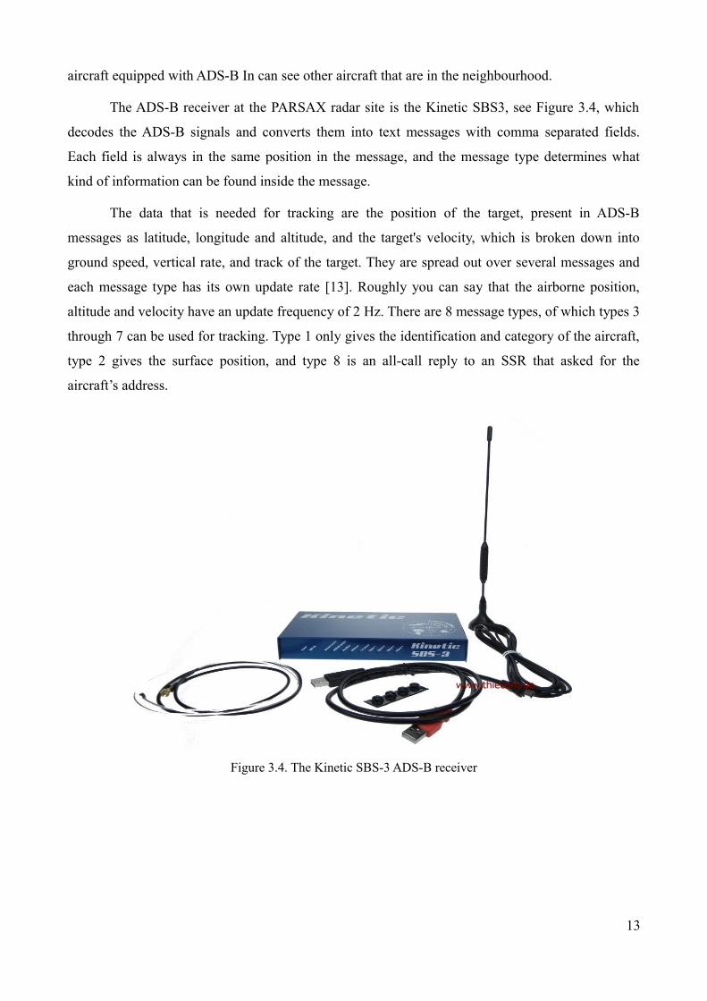
The ADS-B receiver at the PARSAX radar site is the Kinetic SBS3, see Figure 3.4, which

decodes the ADS-B signals and converts them into text messages with comma separated fields.

Each field is always in the same position in the message, and the message type determines what

kind of information can be found inside the message.

The data that is needed for tracking are the position of the target, present in ADS-B

messages as latitude, longitude and altitude, and the target's velocity, which is broken down into

ground speed, vertical rate, and track of the target. They are spread out over several messages and

each message type has its own update rate [13]. Roughly you can say that the airborne position,

altitude and velocity have an update frequency of 2 Hz. There are 8 message types, of which types 3

through 7 can be used for tracking. Type 1 only gives the identification and category of the aircraft,

type 2 gives the surface position, and type 8 is an all-call reply to an SSR that asked for the

aircraft’s address.

Figure 3.4. The Kinetic SBS-3 ADS-B receiver

13

Type 3 is the airborne position message and looks like this:

Type Aircraft Hex-ID Time of Generation Altitude

| | | |

MSG,3,496,211,4CA2D6,10057,2008/11/28,14:53:50.594,2008/11/28,14:58:51.153,,37000,,,

51.45735,-1.02826,,,0,0,0,0

| |

Latitude Longitude

The aircraft Hex-ID is a 6 digit hexadecimal number used to identify the aircraft. The time of

generation can be used to extrapolate the position to the current value. The other time in the

message is the time when the ADS-B receiver sent the message over the network, which is not very

useful here. The altitude is either the true altitude or the pressure altitude, which is not necessarily

equal to the true altitude, see section 3.4.2 for an explanation of the difference. Latitude and

longitude are provided by the on-board GPS device.

Here is an example of a type 4 ADS-B message, which holds the airborne velocity information:

Type Aircraft Hex-ID Time of Generation Ground Speed

| | | |

MSG,4,496,469,4CA767,27854,2010/02/19,17:58:13.039,2010/02/19,17:58:13.368,,,288.6,

103.2,,,-832,,,,,

| |

Track Climb Rate

Ground speed is the speed of the aircraft relative to the ground, given in kts, and the vertical rate is

given in ft/min. The track is the heading of the target in degrees, compensated for the wind. Zero

degrees is in the direction of true north and 90° is due east.

Message types 5 and 6 are triggered by Secondary Surveillance Radars that interrogate aircraft for

their altitude. The reply uses the same frequency as the other ADS-B messages: 1090 MHz.

14

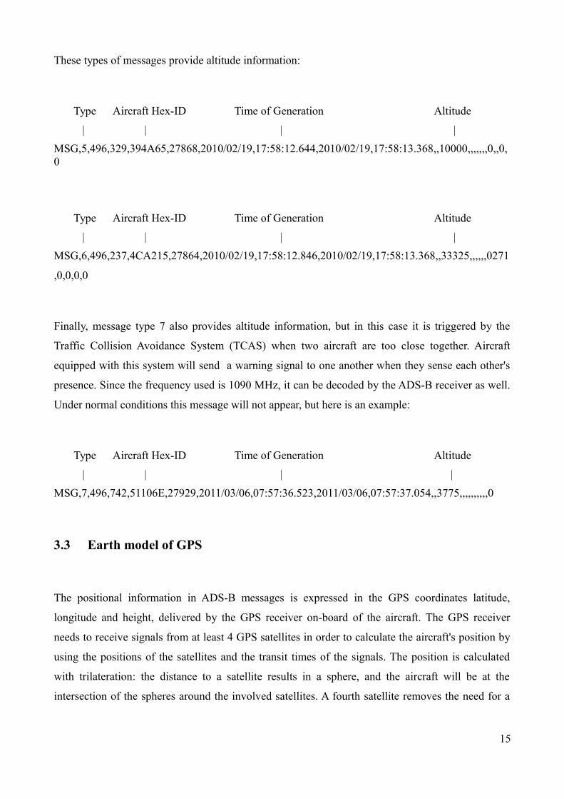
These types of messages provide altitude information:

Type Aircraft Hex-ID Time of Generation Altitude

| | | |

MSG,5,496,329,394A65,27868,2010/02/19,17:58:12.644,2010/02/19,17:58:13.368,,10000,,,,,,,0,,0,0

Type Aircraft Hex-ID Time of Generation Altitude

| | | |

MSG,6,496,237,4CA215,27864,2010/02/19,17:58:12.846,2010/02/19,17:58:13.368,,33325,,,,,,0271

,0,0,0,0

Finally, message type 7 also provides altitude information, but in this case it is triggered by the

Traffic Collision Avoidance System (TCAS) when two aircraft are too close together. Aircraft

equipped with this system will send a warning signal to one another when they sense each other's

presence. Since the frequency used is 1090 MHz, it can be decoded by the ADS-B receiver as well.

Under normal conditions this message will not appear, but here is an example:

Type Aircraft Hex-ID Time of Generation Altitude

| | | |

MSG,7,496,742,51106E,27929,2011/03/06,07:57:36.523,2011/03/06,07:57:37.054,,3775,,,,,,,,,,0

3.3 Earth model of GPS

The positional information in ADS-B messages is expressed in the GPS coordinates latitude,

longitude and height, delivered by the GPS receiver on-board of the aircraft. The GPS receiver

needs to receive signals from at least 4 GPS satellites in order to calculate the aircraft's position by

using the positions of the satellites and the transit times of the signals. The position is calculated

with trilateration: the distance to a satellite results in a sphere, and the aircraft will be at the

intersection of the spheres around the involved satellites. A fourth satellite removes the need for a

15

highly accurate clock in the GPS receiver, which is needed if only three satellites are available.

The earth model of GPS is the World Geodetic System 1984 (WGS84), which is a collection

of models developed by the U.S. Department Of Defence [14]. It describes two models: a geometric

model captures the oblate spheroid shape of the earth, while a physical model relates to the average

level of the oceans. The geometric model describes the shape of the earth as an ellipsoid of

revolution, characterized by the semi-major axis and earth flattening, see Figure 3.5 [15], in which

φ denotes geodetic latitude.

Figure 3.5. Ellipsoidal model of Earth (cross-section normal to equatorial plane)

Points on the earth with equal latitude form circles, of which the equator is an example. Points with

equal longitude, the meridians, are ellipses.

WGS84 is characterized by:

– Semi-major axis a = 6378137 m

– Semi-minor axis b = 6356752.3142 m

– Flattening f = 298.257223563-1

– First eccentricity squared e2 = 2f - f2

16

The physical model Earth Gravitational Model 1996 (EGM96) describes the geoid, which is a

gravitational equipotential surface. There are many of these surfaces, where the gravitational pull of

the earth is constant, but the geoid coincides with the average level of the world oceans, also known

as Mean Sea Level (MSL). It is relatively flat, although there are ridges and valleys, which can be

as much as 100 m apart from the reference ellipsoid.

The third surface is the earth surface, or ground level. Figure 3.6 shows these surfaces;

ground level, the reference ellipsoid, and the geoid.

Figure 3.6. Distances between ground level, geoid, and ellipsoid1

The distance between the earth surface and the reference ellipsoid, designated by the letter h, is the

height a GPS receiver shows. It is the geodetic height, also called Height Above Ellipsoid (HAE).

The orthometric height H equals the distance between ground level and the geoid, and lastly, N is

the geoid height, the local distance between the ellipsoid and the geoid.

In general:

h=H +N (3.4)

1 From http://www.esri.com/news/arcuser/0703/geoid1of3.html, accessed last: June 2014

17

3.4 Calculation of the target position relative to the radar

The azimuth and elevation angle of the target with respect to the radar can be calculated when the

Cartesian distances between them are known. Figure 3.7 shows the calculation of the azimuth and

elevation angle, by using a Cartesian coordinate system centred at the radar site.

Figure 3.7. Calculation of azimuth (left) and elevation (right)

The left diagram shows a top view where the x-axis points east and the y-axis points north. The

diagram on the right is a side view of the target where the x-axis is parallel to the ground and the z-

axis points upward. This coordinate system is known as the ENU (East-North-Up) system. The

problem is however, that the location of an aircraft in an ADS-B message is given in GPS

coordinates, which are centred at the centre of the earth instead of at the radar site. A coordinate

transformation is therefore needed. Section 3.4.1 shows how to perform this transformation, and

the equations to calculate azimuth and elevation of the target with respect to the radar.

The specifications of ADS-B say that the messages can contain both GPS altitude and

pressure altitude. What is needed is the height of the aircraft above PARSAX. Section 3.4.2 gives

the equations to calculate this height for both cases.

18

3.4.1. Calculation of azimuth and elevation

GPS uses an Earth-Centred Earth-Fixed coordinate system, centred at the centre of mass of the

earth. The X-axis goes through the prime meridian and the equator, the Y-axis points east, and the

Z-axis goes through the north pole. Figure 3.8 shows this system in blue, and the ENU system in

green.

Figure 3.8. ECEF and ENU coordinate systems

The radar site is located at the centre of the green square at geodetic coordinates (φR, λR) where φR

is the latitude and λR is the longitude. It is possible to go from ECEF to ENU by translating the

origin from the centre of the earth to the radar site, followed by rotating the axes until they are

aligned [16].

19

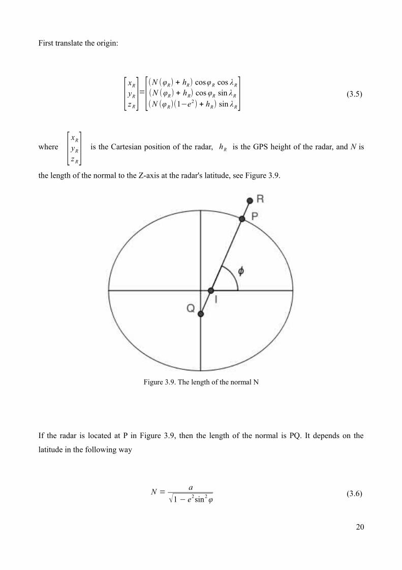
First translate the origin:

[xR

yR

z R]=[

(N (φR) + hR) cosφR cos λR

(N (φR) + hR) cos φR sin λR

(N (φR)(1−e2) + hR) sin λR] (3.5)

where [xR

yR

z R] is the Cartesian position of the radar, hR is the GPS height of the radar, and N is

the length of the normal to the Z-axis at the radar's latitude, see Figure 3.9.

Figure 3.9. The length of the normal N

If the radar is located at P in Figure 3.9, then the length of the normal is PQ. It depends on the

latitude in the following way

N =a

√1 − e2sin2 φ (3.6)

20

The target position in Cartesian coordinates is given by

[xT

yT

zT]=[

(N (φT) + hT) cosφT cos λT

(N (φT ) + hT) cosφT sin λT

(N (φT )(1−e2) + hT) sin λT] (3.7)

Now the target position in local coordinates can be found by using a rotation matrix that rotates the

ECEF axes to align with the ENU axes:

[xT 'yT 'zT ' ]=[

−sin λR cos λR 0−sin φR cos λR −sin φRsin λR cos φR

cosφR cos λR cosφR sin λR sin φR][

xT − xR

yT − yR

zT − z R] (3.8)

The azimuth angle in local (ENU) coordinates of the target with respect to the radar reads

tanα= xT '

yT ' (3.9)

The elevation angle in local coordinates of the target with respect to PARSAX is given by

tan β =zT '

√ xT ' 2+ yT ' 2

(3.10)

Using Eqs. 3.5-3.10, the azimuth and elevation angle of an aircraft with respect to the radar can be

found with the geodetic coordinates of the target and the radar.

21

3.4.2 Calculation of aircraft altitude

From Eq. 3.7 it can be seen that the altitude of the target that is necessary to perform the

calculations is a geodetic altitude. If the ADS-B messages contain GPS altitudes, then they can be

readily used. It is a different matter if the altitude is pressure altitude.

Aircraft are more interested in the difference in altitude between other aircraft than their own

altitude when they are high above the ground. An aircraft calculates its altitude by measuring the

outside air pressure with a device that is calibrated for the International Standard Atmosphere (ISA).

It is a model that describes the relationship with air pressure and temperature as a function of

altitude, based on a standard air pressure of 1013.25 hPa and a temperature of 15ºC. All aircraft use

the same model resulting in accurate relative distances. ADS-B messages can hold both pressure

altitude and true altitude, Figure 3.10 shows the difference between the two.

In the figure the air pressure on the ground is higher than the pressure datum so that the true

altitude is higher than the pressure altitude. Conversely, if there is a low pressure region on the

ground, the pressure datum lies below ground level and the true altitude will be lower than the

pressure altitude.

Figure 3.10. Pressure altitude versus true altitude

22

During take-off or landing, it is important to know the true altitude. The altimeter is then set to the

local air pressure at the airport. The altitude for which the standard pressure datum is used instead

of the air pressure at the airport is called the transition altitude, which is at 3000 ft in Europe.

It is important to have a good estimate of the true altitude to make sure the target is inside

the radar antenna beam. Given that the beam-width of PARSAX is 2.5°, the required altitude

accuracy as a function of range and elevation can be calculated, it is shown in Figure 3.11. Typical

elevation angles for aircraft range from 10° to 50°.

Figure 3.11. Required altitude accuracy as a function of range and elevation

The air pressure outside the aircraft can be found with [17]

p = p0 (1 + τ 0

H b

T 0

)−μgRτ 0 (3.11)

23

where p0 = 1013.25 hPa is the ISA air pressure at sea level,

τ 0 =−6.5⋅10−3 K⋅m−1 is the ISA temperature lapse rate,

H b is the pressure (or barometric) altitude [m],

T 0 = 288.15 K is the ISA temperature at sea level,

μ = 2.89644⋅10−2 kg⋅mol−1 is the molar mass of air,

g = 9.8125 m⋅s−2 is the gravitational acceleration near PARSAX, and

R = 8.31432 J⋅mol−1⋅K−1 is the universal gas constant for air.

Using the outside air pressure, the true altitude can be found by using MSL as the vertical reference

datum:

H =T MSL

τ0

[1 −p

pMSL

]−Rτ 0

μg (3.12)

Using Eq. 3.1, the geodetic altitude of the target is then given by

hT =T MSL

τ0

[1−p

pMSL

]−Rτ 0

μg + N (3.13)

The geoid height N near PARSAX is about 44 m.

Eq. 3.7 needs the geodetic altitude of the target, which is equal to the GPS altitude, and can

be used directly if it is present in the ADS-B messages. If on the other hand, the altitude in the ADS-

B messages is the pressure altitude, then Eqs. 3.12-3.13 will calculate the geodetic altitude of the

target, when the air pressure and temperature on the ground are supplied.

24

3.4.3 Calculation of the slant range

Now that the Cartesian positions of the aircraft and the radar are known, the slant range between

them can be calculated by

R = √(x R − xT)2+ ( yR − yT)

2+ (z R − zT )

2 (3.14)

3.5 Extrapolation of the aircraft position

Because the PARSAX antenna steering system moves relatively slowly, it is necessary to

extrapolate the position of the target in order to calculate where PARSAX can intercept the target

selected for tracking. It is convenient to treat the earth as a sphere, so that the trajectory of a target

with a constant altitude will be an arc of a circle, instead of a part of an ellipse when the WGS84

model is used. The arc will have a radius of Re + hT, where Re is the local radius of the earth, and hT

is the geodetic altitude of the target. The earth radius depends on latitude and can be calculated as

follows:

Re = √(a2cos φR)

2+ (b2 sin φR)

2

(a cos φR)2+ (b sin φR)

2 = 6364900 m (3.15)

where a and b are the semi-major and semi-minor axes, respectively. The velocity components in

the ADS-B messages are ground speed and vertical rate. Ground speed is parallel to the surface of

the earth, and the vertical rate is perpendicular to it. The extrapolation equations then become

φT (t) = φ0 +v⋅t cosθ

Re

λT (t )= λ0 +1

cosφT

v⋅t sin θR e

hT (t) = h0 + vz⋅t

(3.16)

25

where v is the ground speed, vz is the vertical rate (or climb rate), and θ is the track value. It is

assumed that during the observation interval, the ground speed, climb rate, and track are constant.

This is not unreasonable for airliners since this is the case for the most part of the flight. The target

altitude hT is neglected in the first two equations because hT << Re. The factor1

cosφT

in the

second equation of Eq. 3.15 accounts for the fact that the distance between meridians depends on

latitude. A similar factor is unnecessary when extrapolating the latitude, as circles of equal latitude

are equidistant, no matter what the longitude is.

In reality, because of the ellipsoidal shape of the earth, the latitude will differ when a

spherical model is used because the normal will go through the centre of the earth, while with the

ellipsoidal model it will miss it, see Figure 3.12.

Figure 3.12. Difference between geocentric and geodetic latitude

The difference between geocentric and geodetic latitude is exaggerated in the figure, but it is in fact

largest around PARSAX's latitude: about 0.2º. In Eq. 3.16, the geodetic latitude is extrapolated.

Experiments will show if this is allowed, it may be necessary to first convert the geodetic latitude to

geocentric latitude, then extrapolate, and finally convert to geodetic latitude again for further use.

The relation between the two is given by

tan ψ =N (φ)(1 − f )2 + hT

N (φ) + hT

tan φ (3.17)

26

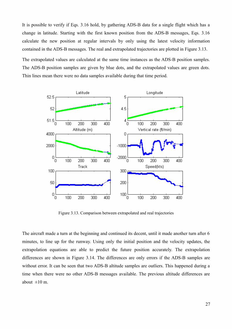
It is possible to verify if Eqs. 3.16 hold, by gathering ADS-B data for a single flight which has a

change in latitude. Starting with the first known position from the ADS-B messages, Eqs. 3.16

calculate the new position at regular intervals by only using the latest velocity information

contained in the ADS-B messages. The real and extrapolated trajectories are plotted in Figure 3.13.

The extrapolated values are calculated at the same time instances as the ADS-B position samples.

The ADS-B position samples are given by blue dots, and the extrapolated values are green dots.

Thin lines mean there were no data samples available during that time period.

Figure 3.13. Comparison between extrapolated and real trajectories

The aircraft made a turn at the beginning and continued its decent, until it made another turn after 6

minutes, to line up for the runway. Using only the initial position and the velocity updates, the

extrapolation equations are able to predict the future position accurately. The extrapolation

differences are shown in Figure 3.14. The differences are only errors if the ADS-B samples are

without error. It can be seen that two ADS-B altitude samples are outliers. This happened during a

time when there were no other ADS-B messages available. The previous altitude differences are

about ±10 m.

27

From Figures 3.13 and 3.14., it is clear that the extrapolation equations 3.16 were able to

predict the future position of the target for several minutes into the future by only using the velocity

information from ADS-B. It is therefore assumed that the equations are correct and that it is allowed

to extrapolate the geodetic latitude directly, without converting to geocentric latitude first.

Figure 3.14. Differences between extrapolated and ADS-B values

3.6 Simulations

To get an idea which flying aircraft PARSAX is able to track, several Matlab simulations were

performed. The ground speed, vertical rate, and track were kept constant, as an airliner behaves like

this most of the time when it is en-route. As seen from the radar, all targets either have a track of

90° when they come from the left, or 270° when they come from the right. Therefore it is only

necessary to regard one track value, plus the starting position of the target relative to PARSAX. The

first simulation only looks at the relative angular velocities of an aircraft with respect to a stationary

point. This will give an indication where aircraft will not be able to be tracked, considering the

28

maximum rotation rate of the PARSAX radar antenna steering system is 36º/min in both angular

directions - azimuth and inclination. The results are shown in section 3.6.1. It is also possible to

simulate tracking an aircraft by PARSAX, using the framework developed in the previous sections.

In this case the coupling of inclination and azimuth of the PARSAX antenna steering system is

taken into account. The results are presented in section 3.6.2.

3.6.1. Relative angular velocities of aircraft

The relative angular velocities of a target with respect to a stationary point is a good indicator of

areas, where PARSAX will have problems with tracking, because of the limited rotation rate of

PARSAX. As previously noted, it is only necessary to regard one flight direction, or track, value

because of symmetry. A track value of 90º is chosen, and the range limit is set to 15 km.

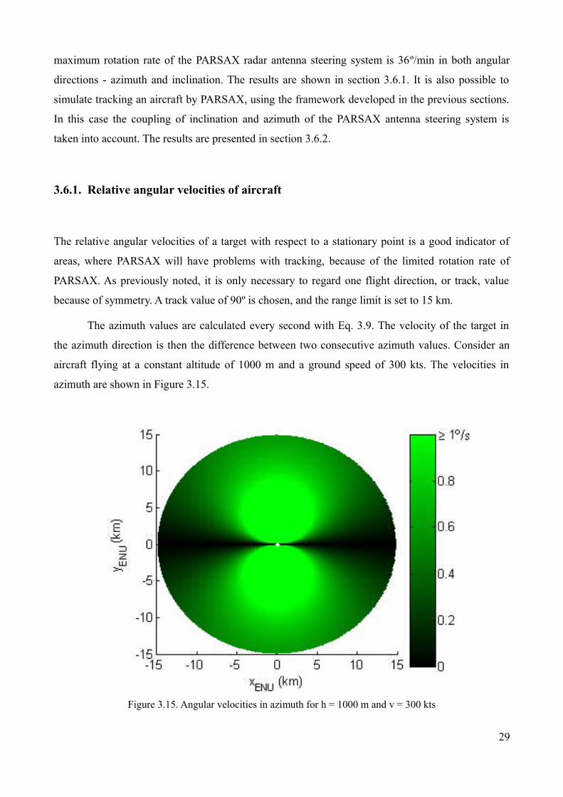
The azimuth values are calculated every second with Eq. 3.9. The velocity of the target in

the azimuth direction is then the difference between two consecutive azimuth values. Consider an

aircraft flying at a constant altitude of 1000 m and a ground speed of 300 kts. The velocities in

azimuth are shown in Figure 3.15.

Figure 3.15. Angular velocities in azimuth for h = 1000 m and v = 300 kts

29

The axes are the ENU axes: the x-axis points east and the y-axis points north. The velocities are

relative to the white dot at the origin. The picture is made of many horizontal flight trajectories from

left to right, since the track is 90º. Starting with a y-value of 0 m, the aircraft flies straight overhead

the origin. The velocity in azimuth is zero, it only rises in elevation at first. Just when it passes

overhead, the azimuth changes from 0º to 180º instantly, giving a momentary peak velocity in

azimuth of 180 º/s. Looking at trajectories with starting y-values above zero, the velocity in

azimuth at the beginning increases, while the maximum velocity, which occurs when the aircraft

crosses the x-axis, decreases. The velocity at the edge of the bright green circle is 1 º/s, already too

fast for PARSAX to follow. The maximum rotation rate of PARSAX is 36 º/min, or 0.6 º/s. Inside

the green circle, the maximum velocity can go up to dozens of degrees per second. It is clear that at

this altitude and speed, PARSAX can possibly track aircraft when they are closing, or when they are

moving away, but not during the entire trajectory. Figure 3.16 shows the velocities in azimuth for an

aircraft flying at a constant altitude of 5000 m and a constant speed of 300 kts.

Figure 3.16. Angular velocities in azimuth for h = 5000 m and v = 300 kts

The angular velocities are identical to the previous case, apparently because an altitude difference of

5 km is insufficient to make a difference. The disc is smaller, as the maximum range is still set at 15

km. It can be seen that it is still impossible for PARSAX to track aircraft during the entire in-range

30

interval. The angular velocities in azimuth for aircraft flying at a constant cruise altitude of 10000 m

and a constant ground speed of 400 kts are shown in Figure 3.17. The velocities at this altitude at

300 kts were the same as in the previous cases. Also, aircraft at the cruise altitude fly approximately

at this speed of 400 kts.

Figure 3.17. Angular velocities in azimuth for h = 10000 m and v = 400 kts

The disc has again become considerably smaller, leaving less time for tracking. The green discs

have become larger as well, as can be expected from the higher ground speed. In any case, it is safe

to say that the maximum velocity in azimuth of an aircraft is too fast for PARSAX to follow. Only

tracking aircraft that are closing, or ones that are moving away from the radar is possible for dozens

of seconds at a time. Especially in the vicinity of the radar.

The same procedure can be applied to plot the angular velocities in elevation. Eq. 3.10 is

used to calculate the elevation angle every second, so that the differences in consecutive values

gives the angular velocity. Figure 3.18 shows the results for an aircraft flying at a constant altitude

of 1000 m and a constant velocity of 300 kts.

31

Figure 3.18. Angular velocities in elevation for h = 1000 m and v = 300 kts

Again the angular velocities are relative to the white dot at the origin. It is clear that the velocities in

elevation are much smaller than the ones in azimuth. The velocities in elevation are symmetrical in

both x- and y-axis, just like the velocities in azimuth, the difference is that the elevation rates are

opposite in sign on both sides of the y-axis. Elevation will rise when an aircraft approaches, and it

will fall when it is moving away. The maximum elevation rates occur when the aircraft passes

straight overhead, with a magnitude of 9 º/s. Trajectories for which yENU > 2200 m have a maximum

angular rate smaller than 0.6 º/s. The elevation angular velocities for an aircraft flying at 5000 m,

and with a ground speed of 300 kts are shown in Figure 3.19.

32

Figure 3.19. Angular velocities in elevation for h = 5000 m and v = 300 kts

The velocities are higher at this altitude than at 1000 m. Trajectories for which yENU > 3700 m have

an angular velocity below PARSAX's maximum rotation rate. Lastly, Figure 3.20 shows the angular

elevation rates for an aircraft at a cruise altitude of 10000 m and a ground speed of 300 kts. In this

case, PARSAX will have no problem tracking the elevation through the entire trajectory when

yENU > 2600 m.

In general, tracking aircraft in elevation is a lot easier than tracking in azimuth. The angular

velocity in azimuth seems to be the bottleneck that causes loss of target when the range is minimal,

for every combination of altitude and ground speed. The best chance for long tracking times is

probably when the minimum range is relatively small. For these trajectories the azimuth velocity

will remain small at first, but on the other hand, the angular rates in elevation will be higher. Section

3.4.2 shows simulations of trajectories where PARSAX itself is taken into account. This will shed

more light on how much tracking time can be expected in reality.

33

Figure 3.20. Angular velocities in elevation for h = 10000 m and v = 300 kts

3.6.2. Simulations of tracking aircraft with PARSAX

The previous section showed the angular velocities of aircraft with respect to a stationary point.

This section presents the results of simulations of PARSAX tracking aircraft. It should provide more

insight into what the impact is of the azimuth offset on tracking duration.

The simulations were performed in Matlab as follows. A target has a constant altitude and a

constant ground speed. It starts out of range of PARSAX with a track of 90º and the position is

extrapolated by Eqs. 3.16. When the range equals the maximum range of 15 km, the time is set to

zero. At this moment PARSAX is positioned so that the target is in the centre of the beam. The

azimuth and elevation angle of the target are calculated by Eqs. 3.9 and 3.10, respectively. Every

second, the aircraft is extrapolated one second ahead. The inclination which corresponds to the new

elevation of the target is calculated by Eq. 3.1. If the difference between the new inclination and the

old one is larger than the maximum rotation rate of 0.6 º/s, PARSAX will add the maximum rate to

the old inclination, otherwise it will assume the new inclination. The corresponding azimuth offset

is obtained from Eq. 3.2, and the azimuth viewing angle from Eq. 3.3. It is assumed that the cables

are not an issue so that PARSAX can rotate freely in the azimuth direction. PARSAX's new azimuth

34

angle is also compared with the old one to prevent moving faster than the maximum rotation rate.

The current viewing angle of PARSAX is compared with the angles of the target to see if it is still

inside the beam. This is done with the following test

(az P − azT)2+ (el P − elT)

2 ⩽(beamwidth2 )

2

(3.18)

where az P is the azimuth viewing angle of PARSAX, azT is the azimuth angle of the target with

respect to the radar, elP is the elevation viewing angle of PARSAX, and elT is the elevation

angle of the target with respect to the radar. For the entire system, a beam-width of 2.5º may be

assumed. To visualize if the target is inside the beam or not, the plots have colours, where green

means that the target is in the centre of the beam, yellow means the target is inside the beam, but not

inside the centre, and when a line is red the target is lost.

Figure 3.21 shows the results of the simulation when tracking a target flying straight

overhead at a constant altitude of 1000 m and a ground speed of 300 kts with a good azimuth offset,

meaning the offset is in the same direction as in which the target moves. The x-axis shows the

transpired time in seconds.

From Figure 3.2 it can be seen that the inclination can be either positive or negative to

achieve the same elevation. The sign of the inclination, together with the track of the target,

determines if the azimuth offset will be good, meaning it will assist in following the target, or not. A

bad offset forces PARSAX to overcome the offset while tracking the target, thus effectively losing

speed.

The top left plot in Figure 3.21 shows the inclination, which is negative because the offset

needs to be good and the target moves towards a higher azimuth, also see Figure 3.3. Right next to

it is the inclination angular rate. It shows that the limited angular rate of PARSAX in inclination is

responsible for not being able to track the aircraft when it goes into the yellow phase once the

inclination saturates.

The middle left plot shows the target azimuth angle as a dashed blue line. The jump from

-90º to 90º is clearly visible. The green-yellow-red line is PARSAX's azimuth viewing angle, and

the azimuth angular rate is shown in the plot right next to it. It shows that saturation only takes

35

place after the target has been lost. The azimuth offset is visible as well; even though the target

azimuth angle is constant, PARSAX needs to counteract the offset to keep its azimuth viewing angle

constant as well.

Figure 3.21. Simulation plots of tracking a target with h = 1000, v = 300, yENU = 0, and good offset

The bottom pair of plots shows the elevation angles of the target and PARSAX on the left,

and the slant range on the right. The rise in elevation is much too steep for PARSAX to follow,

causing loss of target. The range plot shows that the target closes from the maximum range of 15

km, but it is lost before it reaches the minimum range.

Figure 3.22 shows the plots for the same target, but in this case PARSAX has a bad azimuth

offset. Because the target azimuth is constant, the azimuth offset has no effect and the tracking time

will be the same. The only difference is that the inclination and azimuth angular rate have changed

sign.

36

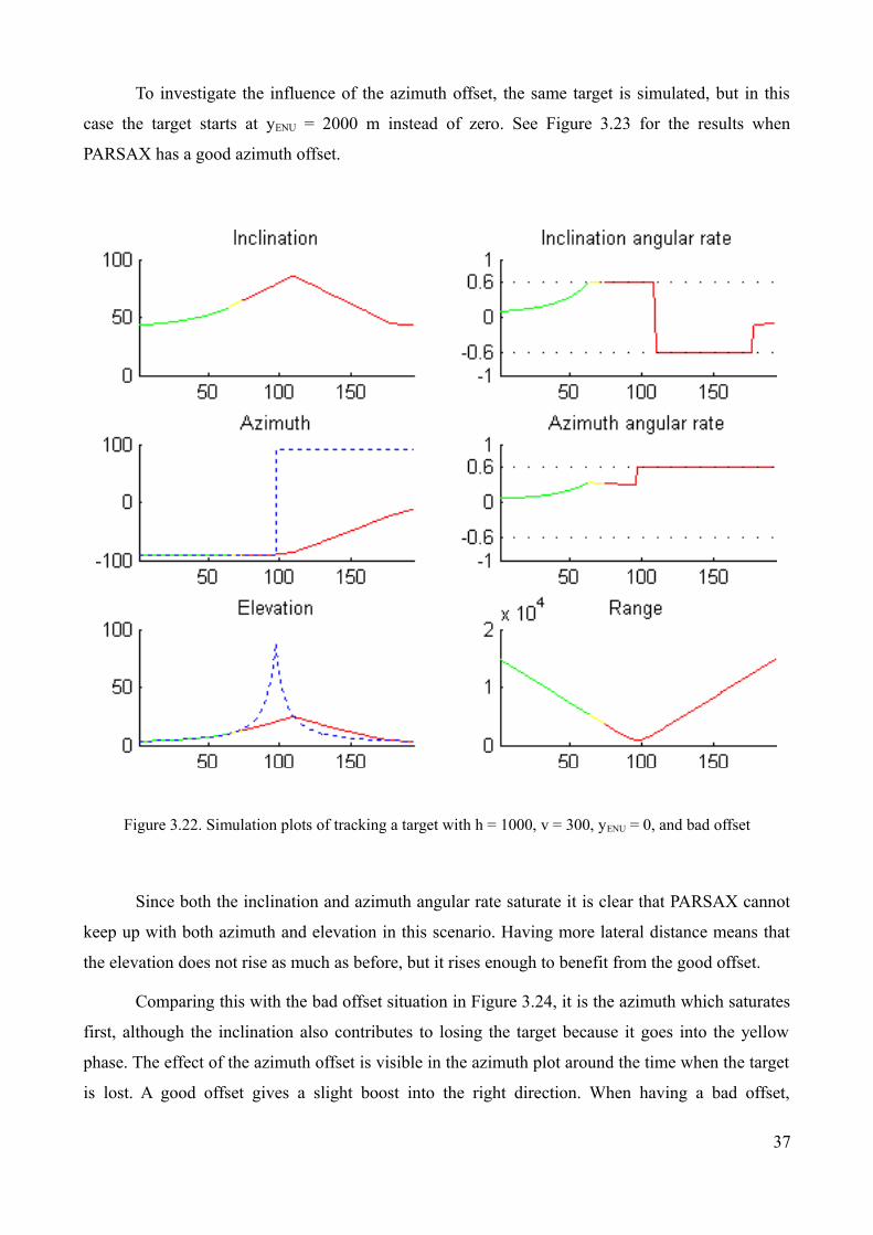
To investigate the influence of the azimuth offset, the same target is simulated, but in this

case the target starts at yENU = 2000 m instead of zero. See Figure 3.23 for the results when

PARSAX has a good azimuth offset.

Figure 3.22. Simulation plots of tracking a target with h = 1000, v = 300, yENU = 0, and bad offset

Since both the inclination and azimuth angular rate saturate it is clear that PARSAX cannot

keep up with both azimuth and elevation in this scenario. Having more lateral distance means that

the elevation does not rise as much as before, but it rises enough to benefit from the good offset.

Comparing this with the bad offset situation in Figure 3.24, it is the azimuth which saturates

first, although the inclination also contributes to losing the target because it goes into the yellow

phase. The effect of the azimuth offset is visible in the azimuth plot around the time when the target

is lost. A good offset gives a slight boost into the right direction. When having a bad offset,

37

PARSAX has to waste speed to overcome the azimuth offset, resulting in 13 seconds less tracking

time in this situation.

Figure 3.23. Simulation plots of tracking a target with h = 1000, v = 300, yENU = 2000, and good offset

When the lateral distance yENU is increased further, there comes a point where the elevation

can be followed without a problem and it is only the change in azimuth that causes a loss of target.

For the current altitude of 1000 m and ground speed of 300 kts, this happens when yENU = 3000 m

with a good offset, see Figure 3.25. If PARSAX has a bad offset, then the elevation can be followed

with no problem when the lateral distance is at least 3000 m as well, although it is the rate in

azimuth that purely causes a loss of target for lower lateral distances as well.

38

Figure 3.24. Simulation plots of tracking a target with h = 1000, v = 300, yENU = 2000, and bad offset

Just as with the simulations of the angular velocities in section 3.4.1, it is possible to show

many trajectories in one plot. Figure 3.26 shows all possible trajectories for a target flying at a

constant altitude of 1000 m and a constant ground speed of 300 kts. PARSAX is located at the white

dot at the origin and starts tracking when an aircraft reaches the maximum range, flying in from the

left. Again, the colours tell where the target is with respect to the beam: green when it is in the

centre of the beam, yellow if it is still inside the beam, but outside the centre because PARSAX

cannot keep up, and red once the target is lost.

39

Figure 3.25. Simulation plots of tracking a target with h = 1000, v = 300, yENU = 3000, and good offset

Figure 3.27 shows a plot of the same trajectories, but this time PARSAX tracks with a bad

offset. Comparing both figures, the advantage of tracking with a good offset is visible by the red

lobes that are less pronounced than the ones when using a bad offset. The result of making these

plots for combinations of altitude, speed, and azimuth offset is presented in Figure 3.28.

The top row shows plots of tracking targets with a good offset and a ground speed of 300

kts, and altitudes of 1000, 5000, and 10000 m, respectively. The circles become smaller because of

the higher altitude, while the maximum range stays the same. The effect of the azimuth offset is

apparent when the plots are compared to the ones in the second row, which have the same

trajectories, only tracked with a bad offset. Tracking times look better for most trajectories, except

for straight overhead, where the offset does not matter.

40

Figure 3.26. Tracking targets with θ = 90º, h = 1000 m, v = 300 kts, and good offset

In the third row are plots of tracking targets with a ground speed of 400 kts this time, a good

offset, and again altitudes of 1000, 5000, and 10000 m, respectively. Because of the higher ground

speed, the relative velocities will be higher, causing loss of target to occur earlier. The last row has

plots of the same trajectories, but tracked with a bad offset. Also for this velocity, the effect of the

azimuth offset is clear. It is also clear that tracking aircraft that are at cruise altitude will not be

possible for long periods of time. The ground speed at these altitudes is usually a little over 400 kts.

41

Figure 3.27. Tracking targets with θ = 90º, h = 1000 m, v = 300 kts, and bad offset

Table 3.1 shows the overhead and maximum tracking time for targets with varying speeds, altitudes,

and azimuth offset. The overhead tracking time is the tracking time for an aircraft that passes

straight overhead. The difference between tracking with a good or bad offset can be as much as 25

seconds, depending on the altitude and ground speed.

Altitude

Ground speed

1 km

300 kts

5 km

300 kts

10 km

300 kts

1 km

400 kts

5 km

400 kts

10 km

400 kts

Overhead 73 44 22 52 26 8

Max. good 76 62 41 54 38 20

Max. bad 74 47 28 52 27 10

Table 3.1. Tracking times for targets at various altitudes, ground speeds, and azimuth offsets

42

Figure 3.28. Tracking simulation for combinations of altitude, speed, and azimuth offset

43

3.7 Tracking aircraft

In conventional tracking, the problem is to determine which radar echo belongs to which target,

while the range and azimuth are measured. The problem in this study resembles the inverse: to

dynamically position the radar given the target ID and its position. The ADS-B signals are provided

at discrete time instances. Between two updates, the state of the target needs to be estimated, given

the last (noisy) update and a model of the target. A target model describes how the target state

evolves in time, given an initial state. At the next measurement, the target state can be updated to a

more accurate value. This is captured by the measurement model. These models are described in

sections 3.7.1 and 3.7.2, respectively. A good way of dealing with state estimation and noisy

measurements is to use a Kalman filter. This is discussed in section 3.7.3. The last section describes

what the tracking algorithm will look like.

3.7.1 Target model

The motion of a target is usually represented by a state-space model,

xk+1 = f k( xk , uk) + w k (3.19)

where xk is the state, uk is the input provided by the (auto)pilot, and w k is the process noise,

all at time instant k [18]. A discrete state space model is given here, because the ADS-B updates

occur at discrete time intervals, and PARSAX will receive move instructions once every second.

Tracking in local coordinates will be difficult, judging from Eqs. 3.9 and 3.10: azimuth and

elevation are highly non-linear and coupled between coordinates. The extrapolation equations 3.16

are a better candidate. Although they are non-linear, they are linear during a short timespan of a

couple of seconds. The update intervals of ADS-B messages are below 1 s, so it is reasonable to

assume that the velocity remains constant during this time. This is actually the case, as shown in

section 3.5. The target model is then a nearly Constant Velocity (CV) model.

44

The state equation then yields

φk+ 1 = φk +vk cos θk

Re

+ wφ

λk+1 = λk +1

cos φk

v k sin θ k

Re

+ w λ

hk+1 = hk + vz + wv

(3.20)

when the state is calculated every second. Note that there is no input, only the state, a constant Re

and the process noise is used.

3.7.2 Measurement model

The measurement equation in general reads

z k = hk (xk ) + vk (3.21)

where z k is the observation and vk is the measurement noise, both at time instant k [19]. The

measurement noise is determined by the GPS error, the resolution of the ADS-B data, and the fact

that it is possible that two ADS-B messages may corrupt each other when they collide at the

receiver. It will have to be estimated in order to get good results.

3.7.3. Kalman filter

An efficient way of dealing with state estimation and noisy measurements is to use a Kalman filter

[20]. It only needs the latest state and measurements to calculate the next estimate, so it can be used

in real time. When the models are correct, the filter will minimize the error covariance. It does this

by assigning weights to the measurements. If the error covariance is small, then the measurements

45

will be trusted and the weights will be high. When on the other hand, the error covariance is large,

then it will rely more on the system equations by making the weights small. A Kalman filter acts

like a predictor-corrector, because the predictions by using the state equations are corrected by the

measurements.

3.7.4 Tracking algorithm

The tracking procedure can be divided into three phases: a surveillance phase, an interception

phase, and a tracking phase.

Surveillance phase

In the surveillance phase all aircraft that are within range of the ADS-B receiver are regarded.

Given the current position and velocity, the position can be extrapolated in order to determine if a

target will be in range in the future. Aircraft that are out of range and will not be in range with the

current track can be dismissed until their track changes. For aircraft that are predicted to be in

range, the tracking intervals can be calculated. The actual expected tracking time can be found by

taking the current radar position into account. First the interception point is calculated, after which

simulating tracking from that point will give an estimate of the tracking time. The calculations can

be performed once per second, as measurements the latest ones will be used. A list with aircraft and

their expected tracking times can be shown for the user to decide which target to track.

Interception phase

A target has been selected and PARSAX is moving towards the position where the target is expected

to be tracked first. During this phase, this position is continuously updated, possibly resulting in a

different starting position for PARSAX and a different total expected tracking time. It is possible

that the current target has become impossible to track because of a turn or that another target is

expected to have a much longer tracking time. In these cases, a different target may be selected and

the interception phase starts again for the new target.

46

Tracking phase

This phase starts with the arrival of the target at the interception point and PARSAX starts moving

along with it. It keeps tracking until the target goes out of range or when an angular velocity

becomes too large and the target is lost. Tracking may also stop when PARSAX cannot rotate any

longer because of the cables. Tracking is made possible by predicting the future position of the

target given its current position and velocity, and measurements from the ADS-B messages. A

Kalman filter should give the best estimates for the states. If the Kalman filter is tuned correctly,

then the estimates it makes will be better than the measurements alone.

3.8 Summary

This chapter analyzed the peculiar movement of the PARSAX antenna steering system. The azimuth

offset induced by the movement in inclination can give a boost to the rotation speed in azimuth, or

reduce it, depending on the attitude of PARSAX and the flight direction of the target.

Calculations are performed in a radar-centred coordinate system, but as the aircraft position

from GPS contained in the ADS-B messages is in earth-centred coordinates, a coordinate

transformation is needed. This transformation allows for simulations which showed the relative

angular velocities with respect to a stationary point. It can be concluded that only closing aircraft, or

aircraft that are moving away may be tracked because of their high maximum angular velocities in

azimuth. The elevation angular velocities pose a lesser problem, especially for aircraft that have a

larger minimum range.

The effect of the azimuth offset on tracking time was studied by simulating aircraft with a

constant velocity. The result was that aircraft may be tracked for dozens of seconds if they are

flying at moderate altitudes, for example aircraft that are preparing to land at Schiphol airport.

Because of the limited rotational speed of the PARSAX antenna, it is necessary to

extrapolate aircraft positions in order to calculate the interception points. The extrapolation

equations were derived by modelling the earth as a sphere, a test with real ADS-B data showed that

this is allowed.

Finally, a tracking algorithm is described which uses a Kalman filter to continuously

estimate aircraft positions and steer the PARSAX antennas.

47

Chapter 4

Implementation

Initial software development was performed in an earlier project [2]. The C# programming

language was used in the project, but because the author is not proficient in that language, the

software for the developed algorithms is written in C++ in the .NET framework. Section 4.1

describes the hardware interfaces that the software should have to control the PARSAX antennas

steering system. The tracking phases, as described in section 3.7.4 are treated in section 4.2. One of

the main functions that needs to be implemented is the function which calculates the estimated

tracking time. Its implementation is described in section 4.3. The Kalman filter that was used is

shown in section 4.4. When pressure altitude is used, the air pressure and temperature are needed in

the calculations, section 4.5 shows where to get this information.

4.1 Hardware interfaces

Besides the radar, there is other hardware that needs interfacing. The system architecture is shown

in Figure 4.1. The hardware is shown on the left, and the software on the right hand side. There is a

camera mounted onto the radar, in the line of sight. The pictures taken by the camera are sent via

the network, where they can be processed by a computer. Image processing performed on these

images is a possibility, when an aircraft is being tracked, or in post-processing. Since it is a pan-tilt-

zoom (PTZ) camera, commands given via the network can make it pan, tilt, or zoom.

The ADS-B receiver continuously decodes the ADS-B messages it receives and sends text

messages over the network. It comes with the Base-station software, in which some settings can be

changed, but the receiver acts basically as a transmitter of ADS-B messages, as far as PARSAX is

concerned.

48

The PARSAX radar has an antenna steering programmable controller which receives,

executes and reports commands from the radar-control software, running on a main host computer

under the Windows 7 OS. This software also controls the current radar configuration (including

transmitted waveforms, power and digital signal processing algorithms), receives data, acquired and

pre-processed with specialized FPGA-based PC boards, for further real-time parallel GPU-based

processing and final storage on hard disks. All range-Doppler processing in four polarimetric

channels of radar is done in real-time. The final goal of this research project is to develop software,

which will be a part of a radar-control package and provide the possibility to collect long time

records of polarimetric signals reflected by tracked flying aircraft.

Figure 4.1. System architecture

4.2 Three phases

In all three phases, the ADS-B receiver delivers text messages in a separate thread. The aircraft list

is updated accordingly. The three phases are surveillance, interception, and tracking. In the

surveillance phase, the expected tracking time of every aircraft in the aircraft list is calculated, and

shown to the user via the user interface. When the user clicks the intercept button, the interception

phase begins.

In the interception phase the estimated tracking time is continuously calculated, also for the

aircraft that is being intercepted, as it is possible that the target will make a turn and the expected

49

tracking time will change. The interception point is calculated at the same time, and PARSAX is

moving toward it at maximum speed. When the user hits the stop button, the interception phase

ends, returning to the surveillance phase. Once the target arrives at the interception point, the

tracking phase begins.

Even in the tracking phase the estimated tracking time is calculated for all aircraft, since it is

possible a better candidate will become available for the user during tracking. What is actually

happening during tracking is depicted in Figure 4.2. The ADS-B receiver relays the messages from

the target. The noisy position and velocity information is filtered by the Kalman filter and it

produces the future position one second ahead. The coordinate transformation calculates the

corresponding inclination and azimuth, which are given to the steering controller, with the correct

speed so that the calculated angles will be reached one second from now. This process is repeated

until the tracking phase ends.

Figure 4.2. Tracking in progress

50

4.3 Implementation of tracking time estimation

This is the main function of the implementation, which uses almost all equations from Chapter 3.

The following steps are taken to find the expected tracking time:

– Calculate the in-range interval. If the interval is empty, return 0.

– In the in-range interval, calculate the interception intervals with a good and a bad azimuth

offset. If the target cannot be intercepted, return 0.

– In the interception interval(s), simulate tracking and return the maximum tracking time.

Section 4.3.1. shows how to calculate the in-range interval. The calculation of the interception

intervals is treated in section 4.3.2, and section 4.3.3 describes how to simulate tracking in the

interception intervals.

4.3.1. Calculating the in-range interval

The range is calculated with Eq. 3.14. If the aircraft is out of range, then the minimum range needs

to be found. If it is larger than PARSAX's maximum range, then it will stay out of range. Trying to

find the minimum of Eq. 3.14 analytically is too complicated, the equations will become quite large.

It will have to be solved numerically. Brent's method is a good way of accomplishing this, it is a

root-finding method that is almost as fast as Newton's method, but it is more robust at the same time

than other methods2 [21]. It uses two inputs for which the function values must be opposite in sign.

Because the minimum range is not known, Brent's method cannot be used yet. The minimum is

found by using the bisection method instead. Suppose the minimum occurs at time T1. The left side

of the in-range interval may now be found by using Brent's method on the function

f = R(t)− Rmin , where Rmin = 15 km is PARSAX's minimum range, and feeding it f (T 0)

and f (T 1) . The right hand side can be found in a similar way, by passing f (T 1) and f (T 2)

to Brent's method, where T2 > T1 is a time for which the target is out of range.

2 http://www.codeproject.com/Articles/79541/Three-Methods-for-Root-finding-in-C, last accessed: June 2014

51

If the target is already in range, then the left side of the interval is zero and the right side of

the interval can be found with Brent's method as described above.

4.3.2. Calculating the interception intervals

An interception point is a point where PARSAX will have the target in the centre of the beam. Both

sides of the interception interval are found by using binary search. There is a separate function that

calculates the rotating time when rotating from one attitude to the next, taking the azimuth offset

and the cables into account. Both intercepting with good and bad offset needs to be looked at,

because tracking with a bad offset may give much more tracking time than tracking with a good

offset, in some cases.

4.3.3. Calculating simulated tracking times

The estimated tracking time for a target that is closing, can be found in the same way as was done in

section 3.6.2, starting from the left part of an interception interval. Since the trajectories are

symmetrical in the yENU-axis, the tracking time for a target that is moving away is the same as for a

target that is closing and that flies to the interception point. Tracking a target that is moving away is

different in that the relative velocity of the target is at maximum at the start, while for a target that is

closing the maximum relative velocity is largest at the end. The tracking time can then be found by

starting at the right side of the interception interval, when the target is in the centre of the beam, and

then tracking backwards in time, until the target is lost. At that point the target will be just outside

the beam, this is the optimal interception point. Some margin needs to be built in though, because if

the tracking starts too soon, PARSAX will not be able to catch up with the target.

4.4 Implementation of the Kalman filter

Because Eqs. 3.20 are non-linear, an Extended Kalman Filter (EKF) is used3, which is a Kalman

filter that works on a linearised version of the state equations. The Kalman filter can be tuned by

3 Taken from http://kalman.sourceforge.net, last accessed: June 2014

52

first gathering ADS-B data for individual flights. By letting the filter estimate the positions and

comparing them with the ADS-B data, the values for the process and measurement noise can be set

to values that give the smallest prediction error.

4.5 Weather information

If pressure altitude is used in the ADS-B messages, then the true altitude can be calculated by Eqs.

3.11 and 3.13, which needs the air pressure and temperature at MSL. METAR messages are short

weather reports for pilots, which also contain air pressure and temperature at an airport4. In reality

the air pressure and temperature right below the aircraft is needed, but this is impossible to get. The

deviation will not be enormous though. The data that is used is for Rotterdam Airport (EHRD),

which is close to the radar site. When the user clicks a button, the report is downloaded, and the air

pressure and temperature is filtered out.

4 http://www.knmi.nl/actueel/metar.html, last accessed: June 2014

53

Chapter 5

Conclusion

The novelty of the research is defined by the study of the ability of the PARSAX radar antenna

steering system to automatically track flying aircraft. The PARSAX radar has quite limited angular

velocities (below 36 degrees per minute in both axes) and is unable to use techniques such as

conical scanning or monopulse. A simulation framework has been developed and intensively used

to study the resulting tracking capability. A method for estimation of radar potential to track aircraft

with specific trajectories and relative location to the radar has been developed. It can be used to

support the radar's operator in the selection of a "trackable" target. As soon as a target is selected for

tracking, a developed Kalman-filter based algorithm uses broadcasted ADS-B information to steer

the radar's antennas continuously in the direction of the flying aircraft.

The developed algorithms have been tested in simulations in the MATLAB environment and

implemented in C++ in the .NET framework for real-time operation in integrated radar-control

software. Unfortunately, full integration and validation of the algorithms have been delayed by the

discovered problems with the PARSAX radar's antennas steering controller firmware (the controller

frequently crashes when antennas move in both axes at the same time). The developed approach,

algorithms and implementation codes are quite general and also can be used with the X-band radar,

which is currently under development of the Microwave Sensing, Signals and Systems section and

has a faster antenna steering system. The analysis of the simulations shows that the system should

be able to automatically track aircraft for dozens of seconds, as was required.

54

List of Acronyms

ADS-B Automatic Dependent Surveillance – Broadcast

AMSL Above Mean Sea Level

ATC Air Traffic Control

ECEF Earth-Centred Earth-Fixed coordinate system

EGM96 Earth Gravitational Model 1996

EKF Extended Kalman Filter

ENU East-North-Up coordinate system

GPS Global Positioning System

HAE Height Above Ellipsoid

ISA International Standard Atmosphere

MSL Mean Sea Level

PARSAX Polarimetric Agile Radar in S- and X-band

PSR Primary Surveillance Radar

SSR Secondary Surveillance Radar

TCAS Traffic Collision Avoidance System

WGS84 World Geodetic System 1984

55

Bibliography

1. Krasnov, O.A., Ligthart, L.P., Zhijian Li, Lys, P., & van der Zwan, F., “The PARSAX - full

polarimetric FMCW radar with dual-orthogonal signals”, EuRAD Radar Conference, pp. 84-

87, Oct. 2008

2. van den Kerkhoff, M., Ontwikkeling van een stedelijk toezichtsysteem v1.0, BSc. Thesis, de

Haagse Hogeschool / Thales, Sept. 2012

3. Wilkerson, B.L., Giggenbach, D., & Epple, B., “Concepts for fast acquisition in optical

communications systems”, Proceedings of the SPIE 6304, 63040A, 2006

4. Da Silva, J.L.R., Brancalion J.F.B., & Fernandes, D., “Data fusion techniques applied to

scenarios including ADS-B and radar sensors for air traffic control”, 12th International Conference on Information Fusion, pp. 1481-1488, July 2009

5. Chaozhu Zhang, & Shuai Shao, “Research on ADS-B target trajectory tracking”, International

Conference on Multimedia Technology (ICMT), pp. 3619-3622, 2011

6. Besada, J.A., Garcia, J., De Miguel, G., Casar, J.R., & Gavin, G., “ADS bias cancellation

based on data fusion with radar measurements”, Proceedings of the Third International

Conference on Information Fusion, vol. 2, July 2000

7. de Vela, G., Alvarez, J.I., Portas, J.B., & Herrero, J.G., “Integration of ADS-B surveillance

data in operative multiradar tracking processors”, 11th International Congres on Information

Fusion, pp. 1-8, July 2008

8. Campbell, S.D., Grappel, R.D., & Flavin, J.M., “Multi-sensor processing for aircraft

surveillance in mixed radar/ADS-B environments”, Tyrrhenian International Workshop on

Enhanced Surveillance of Aircraft and Vehicles, pp. 1-6, Sept. 2008

56

9. Weiyi Liu, Jian Wei, Mengchen Liang, Yi Cao, & Inseok Hwang, “Multi-sensor fusion and

fault detection for air traffic surveillance”, IEEE Transactions on Aerospace and Electronic

Systems, vol. 49, no. 4, pp. 2323-2339, Oct. 2013

10. Gustafsson, F., Gunnarsson, F., Bergman, N., Forssell, U., Jansson, J., Karlsson, R., &

Nordlund, PJ, “Particle filters for positioning, navigation, and tracking”, IEEE Transactions

on Signal Processing, vol. 50, no. 2, pp. 425-437, Feb. 2002

11. Smith, D., & Singh, S., “Approaches to multisensor data fusion in target tracking: A

survey”, IEEE Transactions on Knowledge and Data Engineering (TKDE), vol. 18, no. 12,

pp. 1696-1710, 2006

12. Hall, D.L., & Garga, A.K., “Pitfalls in data fusion (and how to avoid them)”, Proceedings of

Fusion '99, July 1999

13. ICAO, “Technical provisions for Mode S services and Extended Squitter (doc 9871) ”, 2nd

ed. (draft), 2011

14. Department of Defence World Geodetic System 1984 – Its Definition and Relationships with

Local Geodetic Systems, National Imagery and Mapping Agency (NIMA), TR8350.2, Jan. 2000

15. Kaplan, E.D., & Hegarty, C.J., Understanding GPS: Principles and Applications, 2nd ed.,

Norwood: Artech House, Inc., 2006

16. Soler, T., “A compendium of transformation formulas useful in GPS work”, Journal of Geodesy,

72, pp. 482-490, 1998

17. Grigorie, L.T., Dinca, L., & Corcau, J., “Aircrafts' altitude measurement using pressure

information: barometric altitude and density altitude”, WSEAS Transactions on Circuits and

Systems, 7, pp. 503-512, 2010

18. Li, X.R., & Jilkov, V.P., “Survey of maneuvering target tracking - part I: Dynamic models”,

IEEE Transactions on Aerospace and Electronic Systems, vol 39, no. 4, pp. 1333-1364, Oct.

2003

57

19. Li, X.R., & Jilkov, V.P., “Survey of maneuvering target tracking - part III: Measurement

models”, Proc. 2001 SPIE Conference on Signal and Data Processing of Small Targets, pp.

423-446, 2001

20. Brookner, E., Tracking and Kalman Filtering Made Easy, John Wiley & Sons, Inc., New

York, 1998

21. Moré, J.J., & Cosnard, M.Y., “Numerical solution of nonlinear equations”, ACM Trans. Math.

Software, 5, pp. 64-85, 1979

58