tracking simulation based on pi controllers and · pdf filetracking simulation based on pi...

Tracking Simulation Based on PI Controllers and Autotuning

Mats Friman and Pasi Airikka

Metso, Automation Business Segment, Tampere, Finland (e-mail:[email protected])

Abstract: A mechanism for automatic update of tracking simulator parameters is suggested. A trackingsimulator is a simulator, which runs in real time, and which corrects its own behavior (models) bycomparing real process measurements to simulator outputs. Typically, a process simulator, no matter ifstatic or dynamic, cannot adapt its behavior to reality, but the tracking simulator has this ability due to itsintegrated update mechanism. A tracking simulator is commonly used for state estimation of non-linearprocess models (simulation models). The suggested invention utilizes standard PI controllers, whichenables fast update of parameters. A major advantage with the PI controllers is that autotuning can beapplied and, hence, no tuning parameters need to be plucked out of the air. With the proposed innovation,it will be easy to extend an ordinary process simulator to a tracking simulator, which can be used formany purposes, including predictive and fault tolerant control, soft sensors, prediction of future plantbehavior, parameter estimation, and plant optimization.

Keywords: Dynamic Simulation, Tracking Simulation, PI control, Autotuning

1. INTRODUCTION

There are many reasons for using dynamic simulation. Thethreshold for using simulation tools is basically a question ofenthusiasm and motivation since there is a very largeselection of high-quality solvers, modelling tools, andlibraries available for free. Many of these are open source(Fritzson, 2003, Åkesson et al. 2009).

Traditionally, it has been time-consuming and expensive tobuild and maintain simulation models, and this has efficientlyhindered their industrial use in daily operation. This problemis gradually disappearing. More and more engineeringplatforms utilize dynamic simulation already at processdesign phase, and those models could be re-used duringoperation, without any additional cost. Process &Instrumentation diagrams that previously have been used todocument process design are already replaced with dynamicsimulations models. With such systems, simulation modelscan easily be generated from a menu, for free.

Despite the long history of using dynamic simulation, it ismostly used off-line. However, there are really hugeopportunities for using dynamic process models on-line, forexample in monitoring, control, and optimization tasks.

Examples of on-line usage of dynamic models include MPCcontrollers (Richalet et al., 1978) and Kalman Filters(Kalman, 1960). These applications, however, traditionallyemploy linear models. Even though several nonlinear MPCapplications have been reported (Rawlings et al., 1994), theadvantage of non-linear models is not justified with the addedcomplexity in the optimization phase.

Simulation models are seldom re-used as such, e.g. fromtraining simulators. Sometimes a plant may use linear models

for MPC control and nonlinear simulations models foroperator training for the same unit process. In that case, thesame unit process model must be modelled twice.

Process models are built with a wide degree of complexityand accuracy. In order to clarify this aspect, standards havebeen developed. For example fossil fuel power plants havebeen divided into three levels according to their complexityand accuracy (ANSI/ISA, 1993).

A difficulty with simulation models is that the state of theprocess cannot, as such, be copied into the simulator. If we,for example, want to simulate an industrial process from thecurrent state, e.g. to show what will happen in the near future,we should first initialize the state of the dynamic model tomatch the state of the process. This task is far from trivial.Even though some measurements are available on-line, thestate of the dynamic model may depend on some actions thatwere implemented long ago.

One way of estimating the state of the process is to run thesimulator in parallel with the process with the inputs of theprocess connected to the simulator, see Fig. 1a. With thisconnection, the outputs of the process and simulator will,however, usually diverge due to unknown or varyingparameters. To overcome this difficulty, a tracking simulatoris used (Fig. 1b).

IFAC Conference on Advances in PID Control PID'12 Brescia (Italy), March 28-30, 2012 FrA1.4

mailto:[email protected])

Fig. 1a. A process simulator may be connected to a real process andrun in real-time. However, outputs from real process and simulatorwill usually diverge if no update mechanism is used.

Fig. 1b. A tracking simulator is a process simulator with an updatemechanism, which tries to match simulator outputs with real processoutputs.

A tracking simulator is a simulator that is run in real-time, inparallel to the process. It utilizes process measurements toupdate its states and parameters, so that simulator outputs andprocess measurements converge.

A problem with tracking simulators is that the adaptingmechanism may be slow due to the primitive updatemechanism used. It is common to use a mechanism thatupdates parameters with an amount proportional to thedeviation between simulator and process measurement.Although being simple, this mechanism is sometimes veryslow. Another problem is the selection of the numericalvalues for the update, since they are usually tuned with trialand error.

In this paper we present an innovative solution, whichovercomes the problems discussed above. We use PIcontroller for speeding up the estimation of simulation modelparameters, and we use autotuning (Åström and Hägglund,1984) techniques to make the parameter selection elegant andsystematic. We believe that the solution suggested here willbe useful when the use of dynamic simulation in dailyoperation will grow.

2. PROPOSED STRUCTURE

Before describing the proposed solution we justify outapproach with a very simple motivating example. Despitebeing simple, it well demonstrates the drawbacks with currenttracking simulators.

2.1 Motivating Example: Cooling Coffee

We use a simplified example to justify our idea and todemonstrate the problems with known technology. Theexample simulates cooling of coffee (Fig. 2), with an initialtemperature of 60 °C and the surrounding room temperaturealternating around 20 °C with the amplitude of 5 °C, andperiod of 600 s. The dynamics is a quite typical first-ordersystem with the coffee temperature being the state variable.

Fig. 2. Cooling Coffee example. The purpose is to estimate roomtemperature (TR) by comparing real (TC,mes)and simulated coffeetemperatures (TC,sim). The simulation block ("Model") updatescoffee temperature based on estimation of room temperature, whichis estimated in the update block ("Update").

The dynamics of the system is described with the equation

CRC TT

dtdT (1)

where variable T denotes temperature, with subscripts R forroom and C for coffee. is a time constant, which is assumedto be known ( = 120 s).

Next we will show how we estimate (update) roomtemperature (TR) by comparing real and simulated coffeetemperatures. According to known technology (see e.g.Nakaya et.al, 2008) a parameter may be updated according to

)()1()( kKekpkp (2)

where e(k) is the deviation (difference) between simulatedand measured value (at time instant k) and K is an updateconstant. The parameter p(k) updates its value based on itsprevious value p(k-1). The approach suggested in this paperuses decentralized PI control, i.e.

))(())1()(()1()( keTK

kekeKkpkpi

pp

(3)


where Kp and Ti are PI controller parameters.

The results of a Cooling Coffee simulation experiment, wherethe two alternative update mechanisms (Eq. 2 and Eq.3) havebeen used, are shown in Fig.3-4. The update constants whereK = -0.1667 for the conventional (Eq. 2) and Kp = -4; Ti = 10for the method suggested in this paper (Eq. 3). The samplingtime was 15 s, and the measurement was delayed with onesample in order not to favour gain selection close to infinity.

From Fig. 3 and 4 we conclude that we get a faster estimationof room temperature by using the update mechanism inspiredby a PI controller (Eq. 3) compared to the single-parameterupdate mechanism according to Eq. 2.

0 200 400 600 800 1000 1200 1400 1600 180015

20

25

30

35

40

45

50

55

60

Time

T C

MeasuredSimulated (Conventional)Simulated (Suggested)

Fig. 3. Simulations of coffee temperature, where the roomtemperature has been updated with Eq.(2) (dashed-line) and Eq.(3)(solid line). The real measured temperature (dotted line) is includedfor reference.

0 200 400 600 800 1000 1200 1400 1600 180014

16

18

20

22

24

26

Time

T R

Real ValueEstimated(Conventional)Estimated (Suggested)

Fig. 4. Estimation of room temperature in the Cooling Coffeeexample, where the room temperature has been updated with Eq.(2)(dashed-line) and Eq.(3) (solid line). The unknown roomtemperature (dotted line) is included for reference.

2.2 General Structure

The motivating example introduced some benefits (mostnotably the speed of update) of using PI controllers fortracking simulation. A block diagram of the suggestedtracking simulator is shown in Fig.5.

Fig. 5. A tracking simulator update mechanism applied with PIcontrollers. The connections to PI controller terminals are thefollowing: process measurement is connected to PI setpoint;simulator output is connected to PI measurement; estimatedparameter is PI control signal. An autotuner is used to tune the PIcontroller parameters.


As seen from Fig. 5, there is a simulator running in parallelwith the process. The inputs to the process are connected tothe simulator. The PI controllers are connected as follows:

outputs of the process, usually processmeasurements (controlled and uncontrolled) areconnected to PI controllers setpoints

outputs of the simulator (corresponding processmeasurements) are connected to PI controllersmeasurements

the output (control value) of the PI controller is theunknown parameter, which will be used by thesimulator

Above we already discussed that a (momentary) drawback ofthe suggested update mechanism is that we need twoparameters instead of one. However, since we have describedthe tracking simulation problem as a control problem, whichcan be solved with decentralized PI control, we can useautotuning, which eliminates the need of manual parameterselection.

2.3 Summary of Implementation

Next we will shortly summarize the implementation from apractical point of view. We use the 3-input-2-output processshown in Fig. 6. as an example process. Two inputs areknown (solid lines) and one is unknown (dashed line).Moreover, there are unknown process parameters, but sincethere are only two measured outputs, we can only estimateone parameter in addition to the unknown input.

Fig. 6. An example 3-input-2-output process. One unknown input(dashed line) and one unknown parameter are identified with two PIcontrollers.

The implementation of the tracking simulator is done asfollows. We assume that a simulator that matches the realprocess is available.

1. Known process inputs (controls) are connected tosimulator.

2. Selected unknown inputs/parameters are connectedto PI controllers. All PI controllers are in manualmode with output equal to an educated guess of theparticular input/parameter.

3. Ad hoc values are used for all otherinputs/parameters.

4. Each PI controller measurement is connected to asimulator output and PI controller setpoint isconnected to corresponding process measurement.

5. Each PI controller is autotuned and connected toautomatic.

6. Some PI controllers may need retuning because ofinteractions between control loops.

In practice, input flows of industrial processes are usuallyknown (e.g. valve positions), but properties of input flows,e.g. temperature, concentrations, pressure, are oftenunknown.

2.4 Alternatives to PI control: The Nelder-Mead and the MITMethods

It is well known that PI controllers can only be used when thesign of process gain is known and does not change with time.In the Cooling Coffee example, where we tried to estimatethe room temperature, it was clear that a higher roomtemperature implies a higher coffee temperature (ie. it has apositive process gain). Modest changes in the magnitude aretolerated, but constant sign of the gain is a prerequisite forsuccessful PI control. However, this is not always guaranteedin the parameter estimation task, and hence other solutionsmust be on hand for the tricky cases. One possible solution isto apply the well known Nelder-Mead algorithm (Nelder andMead, 1965).

Another alternative is to apply the MIT rule, which is wellknown from adaptive control theory (see e.g. Åström andWittenmark, 1989). Here the idea is to multiply the error seenby the PI controller with the "sensitivity derivative". In thatcase, gains and time constants may successfully be estimatedwith PI controllers.

3. INDUSTRIAL EXAMPLE

We will use an economizer from a biomass fired power plantas an example. The economizer is a heat exchanger thatutilizes hot flue gases in order to warm up the feed water.

The model has 13 inputs (parameters are also counted asinputs): temperature before economizer (feed water and fluegas), pressure drop over heat exchanger (feed water and fluegas), specific heat capacity (feed water and flue gas), heat


transfer coefficient, density (feed water and flue gas), totalheat exchanger volume (feed water and flue gas), capacityvalue (i.e. volumetric flow obtained by a pressure drop of 1bar) (feed water and flue gas). There are two outputs, i.e.output temperatures (feed water and flue gas).

Real industrial data, collected from a biomass powered boilerwas used in the examples.

With two outputs in the model, and corresponding processmeasurements, we can update two unknown parameters. Wechose to update the following two parameters: 1) the heattransfer coefficient, because it is useful to know frommaintenance and economic perspective and 2) the specificheat capacity of flue gas because it has a large impact on themodel and large variations in the data due to variation ofmoisture content in the biomass fuel.

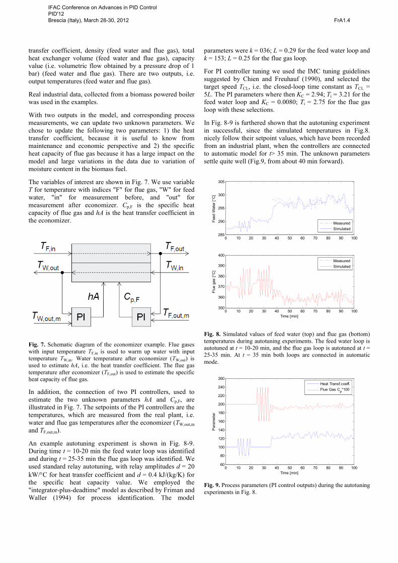
The variables of interest are shown in Fig. 7. We use variableT for temperature with indices "F" for flue gas, "W" for feedwater, "in" for measurement before, and "out" formeasurement after economizer. Cp,F is the specific heatcapacity of flue gas and hA is the heat transfer coefficient inthe economizer.

Fig. 7. Schematic diagram of the economizer example. Flue gaseswith input temperature TF,in is used to warm up water with inputtemperature TW,in. Water temperature after economizer (TW,out) isused to estimate hA, i.e. the heat transfer coefficient. The flue gastemperature after economizer (TF,out) is used to estimate the specificheat capacity of flue gas.

In addition, the connection of two PI controllers, used toestimate the two unknown parameters hA and Cp,F, areillustrated in Fig. 7. The setpoints of the PI controllers are thetemperatures, which are measured from the real plant, i.e.water and flue gas temperatures after the economizer (TW,out,mand TF,out,m).

An example autotuning experiment is shown in Fig. 8-9.During time t = 10-20 min the feed water loop was identifiedand during t = 25-35 min the flue gas loop was identified. Weused standard relay autotuning, with relay amplitudes d = 20kW/ C for heat transfer coefficient and d = 0.4 kJ/(kg/K) forthe specific heat capacity value. We employed the"integrator-plus-deadtime" model as described by Friman andWaller (1994) for process identification. The model

parameters were k = 036; L = 0.29 for the feed water loop andk = 153; L = 0.25 for the flue gas loop.

For PI controller tuning we used the IMC tuning guidelinessuggested by Chien and Freuhauf (1990), and selected thetarget speed TCL, i.e. the closed-loop time constant as TCL =5L. The PI parameters where then KC = 2.94; Ti = 3.21 for thefeed water loop and KC = 0.0080; Ti = 2.75 for the flue gasloop with these selections.

In Fig. 8-9 is furthered shown that the autotuning experimentin successful, since the simulated temperatures in Fig.8.nicely follow their setpoint values, which have been recordedfrom an industrial plant, when the controllers are connectedto automatic model for t> 35 min. The unknown parameterssettle quite well (Fig.9, from about 40 min forward).

0 10 20 30 40 50 60 70 80 90 100285

290

295

300

305

Feed

Wat

er [°

C]

MeasuredSimulated

0 10 20 30 40 50 60 70 80 90 100350

360

370

380

390

400

Flue

gas

[°C

]

Time [min]

MeasuredSimulated

Fig. 8. Simulated values of feed water (top) and flue gas (bottom)temperatures during autotuning experiments. The feed water loop isautotuned at t = 10-20 min, and the flue gas loop is autotuned at t =25-35 min. At t = 35 min both loops are connected in automaticmode.

0 10 20 30 40 50 60 70 80 90 10060

80

100

120

140

160

180

200

220

240

260

Time [min]

Par

amet

er

Heat Transf.coeff.Flue Gas Cp*100

Fig. 9. Process parameters (PI control outputs) during the autotuningexperiments in Fig. 8.


4. CONCLUSIONS

In this paper we have suggested and tested the idea of usingPI controllers for tracking simulation, instead of the wellknown simple update mechanism in Eq. 2. We havesuccessfully tested the idea with a decentralized 2x2 controlsystem. However, results not shown here have demonstratedthat the idea can be applied also on larger systems. In fact,since the idea is similar to ordinary decentralized control, wesee no limitations in the number of parameters that can beupdated according to the ideas presented here.

The parameter identification is, however, not as easy asdecentralized control. In many cases there are parameters thatdo not have a clear direction. For example, in the CoolingCoffee example it was clear that the room temperature has apositive impact on coffee temperature. However, if our taskhad been to estimate the time constant, it would not bepossible to apply PI control (Eq. 3) nor known technology(Eq. 2). However, we can use the MIT rule, which is wellknown from adaptive control, or a slower but more generalsolution, such as the Nelder-Mead algorithm.

Moreover, there are no structural requirements on thesimulation models. The presented idea may be used onODE/PDE/DAE models regardless of properties, such asmodel size, complexity, accuracy, and solver.

There are some open questions related to decentralizedcontrol, including variable pairing, decoupling, stability,closed-loop performance, and control structures (e.g. ratioand cascade controllers). However, since those challenges arebasically identical to those of decentralized process control,we have not discussed these issues in detail. We basicallynotice two main differences between our approach andtraditional decentralized process control. 1) Since processesare never designed with parameter estimation in mind, it isexpected that the process, as seen by the controllers used fortracking simulation, may be very nonlinear. This problem isbest handled by using modest target speed during controllertuning for the loops that enclose nonlinear behaviour. 2) It isimportant to understand the characteristics of each parameterduring tuning and select the control speed accordingly. Forexample, if we are estimating a parameter that changesslowly (e.g. a heat transfer coefficient), we can favourableselect a very sluggish target speed for the controller, andwhen we are updating some rapidly changing phenomena(usually some unknown property of input flows) we shoulduse more aggressive controller tuning.

REFERENCES

Åkesson J., Gäfvert, M., Tummescheit, T. (2009). JModelica- an Open Source Platform for Optimization of ModelicaModels. Proceedings of MATHMOD 2009 - 6th ViennaInternational Conference on Mathematical Modelling,Vienna, Austria.

ANSI/ISA-77.20-1993 (1993), Fossil Fuel Power PlantSimulators - Functional Requirements, Approved 1993,43 p., North Carolina, Instrument Society of America.

Åström, K. J. and Hägglund, T. (1984). Automatic Tuning ofSimple Regulators with Specifications on Phase andAmplitude Margins. Automatica, 20, 645-651.

Åström, K. J. and Wittenmark, B. (1989). Adaptive Control.Addison Wesley.

Chien, I. L. and Freuhauf, P. S. (1990). Consider IMCTuning to Improve Performance. Chem. Eng. Progr.1990 Oct., 33-41

Friman, M. and Waller K.V. (1994). Autotuning of MultiloopControl Systems. Ind.Eng.Chem.Res, Vol. 33, No. 7.

Fritzson, P. (2003). Principles of Object-Oriented Modelingand Simulation with Modelica 2.1, Wiley-IEEE Press,ISBN 0-471-471631.

Nakaya, M., Seki, T., Kawaguchi, K., Onoe, Y., Ootani, T.(2008). Model Parameter Estimation by TrackingSimulator for the Innovation of Plant Operation.Proceedings of the 17th IFAC World Congress, p. 2168-2173, Seoul, Korea.

Nelder, J. A. and Mead, R. (1965). A simplex method forfunction minimization. Computer Journal 7: 308–313.

Kalman, R. E. (1960) A New Approach to Linear Filteringand Prediction Problems. Transaction of the ASME—Journal of Basic Engineering, pp. 35-45.

Rawlings, J. B., E. S. Meadows, and K. R. Muske, (1994).Nonlinear Model Predictive Control: A Tutorial andSurvey ,Proceedings of ADCHEM ’94, 203-214, Kyoto,Japan

Richalet, J. A., A Rault, J. D. Testud, and J. Papon, (1978).Model Predictive Heuristic Control: Application toIndustrial Processes, Automatica, 13, 413


tracking simulation based on pi controllers and · pdf filetracking simulation based on pi...

Documents