tracking - university of torontojepson/csc2503/tracking.pdf · tracking goal: fundamentals of...

Tracking

Goal: Fundamentals of model-based tracking with emphasis on

probabilistic formulations. Examples include the Kalman filter for

linear-Gaussian problems, and maximum likelihood and particle fil-

ters for nonlinear/nonGaussian problems.

Outline

• Introduction• Bayesian Filtering / Smoothing• Likelihood Functions and Dynamical Models• Kalman Filter• Nonlinear/NonGaussian Processes• Hill Climbing (Eigen-Tracking)• Particle Filters

Readings: Chapter 17 of Forsyth and Ponce.Matlab Tutorials: motionTutorial.m

2503: Tracking c©D.J. Fleet & A.D. Jepson, 2009 Page: 1

Challenges in Tracking

Tracking is the inference object shape, appearance, and motion as a

function of time.

Main players:

• what to model or estimate: shape (2D/3D), appearance, dynamics

• what to measure: color histograms, edges, feature points, flow, ...

Some of the main challenges:

• objects with many degrees of freedom,

affecting shape, appearance, and motion;

• impoverished information due to occlusion or scale;

• multiple objects and background clutter

space / aerospace surveillance

smart toys automatic control

sports / kinesiology human motion capture

non-rigid motions biology (animal/cell/molecular)

2503: Tracking Page: 3

Probability and Random Variables

A few basic properties of probability distributions will beused often:

• Conditioning (factorization):

p(a, b) = p(a|b) p(b) = p(b|a) p(a)

• Bayes’ rule:

p(a|b) =p(b|a) p(a)

p(b)

• Independence:a andb are independent if and only if

p(a, b) = p(a) p(b)

• Marginalization:

p(b) =

∫

p(a, b) da , p(b) =∑

a

p(a, b)

2503: Tracking Notes: 4

Probabilistic Formulation

We assume a state space representation in which time is discretized,

and astatevector comprises all variables one wishes to estimate.

State: denotedxt at timet, with the state historyx1:t = (x1, ..., xt)

– continuous variables (position, velocity, shape, size, ...)

– discrete variables (number of objects, gender, activity, ...)

Observations: the data measurements (images) with which we con-

strain state estimates, based on observation equationzt = f(xt).

The observations history is denotedz1:t = (z1, ..., zt)

Posterior Distribution: the conditional probability distribution over

states specifies all we can possibly know (according to the model)

about the state history from the observations.

p(x1:t | z1:t) (1)

Filtering Distribution: often we only really want the marginal pos-

terior distribution over the state at the current time giventhe ob-

servation history. This is called the filtering distribution:

p(xt | z1:t) =

∫

x1

· · ·

∫

xt−1

p(x1:t | z1:t) (2)

Likelihood and Prior: using Bayes’ rule we write the posterior in

terms of alikelihood, p(z1:t | x1:t), and aprior, p(x1:t):

p(x1:t | z1:t) =p(z1:t | x1:t) p(x1:t)

p(z1:t)


Model Simplifications

The distributionp(x1:t), called aprior distribution, represents our

prior beliefs about which state sequences (e.g., motions) are likely.

First-order Markov modelfor temporal dependence (dynamics):

p(xt | x1:t−1) = p(xt | xt−1) (3)

The order of a Markov model is the duration of temporal dependence

(a first-order model requires past states up to a lag of one time step).

With a first-order Markov model one can write the distribution over

the state history as a product of transitions from one time tothe next:

p(x1:t) = p(xt | xt−1) p(x1:t−1)

= p(x1)

t∏

j=2

p(xj | xj−1) (4)

The distributionp(z1:t | x1:t), often called alikelihoodfunction, repre-

sents the likelihood that the state generated the observed data.

Conditional independenceof observations:

p(z1:t | x1:t) = p(zt | xt) p(z1:t−1 | x1:t−1)

=

t∏

τ=1

p(zτ | xτ) (5)

That is, we assume that the observations at different times are inde-

pendent when we know the true underlying states (or causes).


Filtering and Prediction Distributions

With the above model assumptions, one can express the posterior dis-

tribution recursively:

p(x1:t | z1:t) ∝ p(z1:t | x1:t) p(x1:t)

=t∏

τ=1

p(zτ | xτ) p(x1)t∏

j=2

p(xj | xj−1)

∝ p(zt | xt) p(xt | xt−1) p(x1:t−1 | z1:t−1) (6)

Thefiltering distributioncan also be written recursively:

p(xt | z1:t) =

∫

x1

· · ·

∫

xt−1

p(x1:t | z1:t)

= c p(zt | xt) p(xt | z1:t−1) (7)

with aprediction distributiondefined as

p(xt | z1:t−1) =

∫

xt−1

p(xt | xt−1) p(xt−1 | z1:t−1) (8)

Recursion is important:

• it allows us to express the filtering distribution at timet in terms

of the filtering distribution at timet−1 and the evidence at timet.

• all useful information from the past is summarized in the previous

posterior (and hence in the prediction distribution).

Without recursion one may have to store all previous images to com-

pute the the filtering distribution at timet.


Filtering and Smoothing

Provided one can invert the dynamics equation, one can also perform

inference (recursively) backwards in time:

p(xτ | zτ :t) = c p(zτ | xτ )

∫

xτ+1

p(xτ | xτ+1) p(xτ+1 | zτ+1:t)

= c p(zτ | xτ ) p(xτ | zτ+1:t)

That is, the distribution depends on the likelihood the current data,

the inverse dynamics, and the filtering distribution at timet + 1.

Smoothing distribution(forward-backward belief propagation):

p(xτ | z1:t) =c

p(xτ)p(zτ | xτ ) p(xτ | z1:τ−1) p(xτ | zτ+1:t) (9)

The smoothing distribution therefore accumulates information from

past, present, and future data.

Batch Algorithms: Estimation of state sequences using the entire

observation sequence (i.e., using all past, present & future data):

• the filter-smoother algorithm is efficient, when applicable.

• storage/delays make this unsuitable for many tracking domains.

Online Algorithms: Recursive inference (7) is causal. Estimation

of xt occurs as soon as observations at timet are available, thereby

using present and past data only.


Likelihood Functions

There are myriad ways in which image measurements have been used

for tracking. Some of the most common include:

• Feature points: E.g., Gaussian noise in the measured feature

point locations. The points might be specifieda priori, or learned

when the object is first imaged at time 0.

• Image templates:E.g., subspace models learned prior to track-

ing, or brightness constancy as used in flow estimation.

• Color histograms: E.g., mean-shift to track modes of local color

distribution, for robustness to deformations.

• Gradient histograms: E.g., histograms of oriented gradients (HOG)

in local patches to capture image orientation structure as afunc-

tion of spatial position over target.

• Image curves (or edges): E.g., with Gaussian noise in measured

location normal to the contour.


Temporal Dynamics

We often assume a combination of deterministic and stochastic dy-

namics. Common linear models include:

• Random walk with zero velocity and IID Gaussianprocess noise:

xt = xt−1 + ~ηd , ~ηd ∼ N (0, C)

• Random walk with zero acceleration and Gaussianprocess noise(

xt

~vt

)

=

(

1 1

0 1

) (

xt−1

~vt−1

)

+

(

~ηd

~ǫd

)

where~ηd ∼ N (0, Cx) and~ǫd ∼ N (0, Cv) .

• For higher-order models we define an augmented state vector,and

then use a first-order formulation. E.g., for a second-ordermodel:

xt = Axt−1 + Bxt−2 + ~ηd

one can define

~yt ≡

(

xt

xt−1

)

for which the equivalent first-order augmented-state modelis

~yt =

(

A B

I 0

)

~yt−1 +

(

~ηd

0

)

Typical observation model:zt =f( [I 0] · ~yt) plus Gaussian noise.


Dynamical Models

There are many other useful dynamical models. For example, harmonic oscillation can be expressed

as

d2x

dt2= −x

or as a first order system with

d~u

dt=

(

0 1

−1 0

)

~u , where ~u ≡

(

x

v

)

A first-order approximation yields:

~ut = ~ut−1 + ∆td~u

dt+

(

η

ǫ

)

=

(

1 ∆t

−∆t 1

)

~ut−1 +

(

η

ǫ

)

In many cases it is useful to learn a suitable model of state dynamics. There are well-know algo-

rithms for learning linear auto-regressive models of variable order.


Kalman Filter

Assume a linear dynamical model with Gaussianprocess noise, and

a linear observation model with Gaussianobservation noise:

xt = A xt−1 + ~ηd , ~ηd ∼ N (0, Cd) . (10)

zt = M xt + ~ηm , ~ηm ∼ N (0, Cm) (11)

The transition densityis therefore Gaussian, centred at meanA xt−1,

with covarianceCd :

p(xt | xt−1) = G(xt; A xt−1, Cd) . (12)

Theobservation densityis also Gaussian:

p(zt | xt) = G(zt; M xt, Cm) . (13)

Because the product of Gaussians is Gaussian, and the marginals of a

Gaussian are Gaussian, it is straightforward (but tedious)to show that

the prediction and filtering distributions are both Gaussian:

p(xt | z1:t−1) =

∫

xt−1

p(xt | xt−1) p(xt−1 | z1:t−1) = G(xt; x−t , C−t ) (14)

p(xt | z1:t) = c p(zt | xt) p(xt | z1:t−1) = G(xt; x+t , C+

t ) (15)

with closed-form expressions for the meansx−t , x+t and covariances

C−t , C+

t .


Kalman Filter

Depiction of Kalman updates:

deterministic drift

stochasticdiffusion

incorporate data

posterior at t-1

posterior at t prediction at t

data


Kalman Filter (details)

To begin, suppose we know thatx ∼ N (~0, C), and let~y = Ax. Sincex is zero-mean, it is clear that

~y will also be zero-mean. Further, the covariance of~y is given by

E[ ~y~yT ] = E[ A xxT AT ] = A E[ xxT ] AT = A C AT (16)

Now, let’s use this to derive the form of the prediction distribution. Let’s say that we know the

filtering distribution from the previous time instant,t−1, and let’s say it is Gaussian with meanx+t−1

with covarianceC+t−1.

p(xt−1 | z1:t−1) = G(xt−1; x+t−1, C+

t−1) . (17)

And, as above, we assume a linear-Gaussian dynamical model,

xt = A xt−1 + ~ηd , ~ηd ∼ N(0, Cd) . (18)

From above we know thatA xt−1 is Gaussian. And we’ll assume that the Gaussian process noise~ηd

is independent of the previous posterior distribution. So,18 is the sum of two independent Gaussian

random variable, and hence the corresponding density is just the convolution of their individual

densities. Remember that the convolution of two Gaussians with covariancesC1 andC2 is Gaussian

with covarianceC1 + C2. With this, it follows from (17) and (18) that the predictionmean and

covariance ofp(xt | z1:t−1) in (14) are given by

x−

t = A x+t−1 , C−

t = A C+t−1A

T + Cd .

This gives us the form of the prediction density.

Now, let’s turn to the filtering distribution. That is, we wish to combine the prediction distribution

with the observation density for the current observation,zt, in order to form the filtering distribution

at timet. In particular, using (15), with (13) and the results above,it is straightforward to see that

p(xt | z1:t) ∝ p(zt | xt) p(xt | z1:t−1) (19)

= G(zt; Mxt, Cm) G(xt; x−

t , C−

t ) . (20)

Of course the product of two Gaussians is Gaussian; and it remains to work out expressions for its

mean and covariance. This requires somewhat tedious algebraic manipulation.

While there are many ways to express the posterior mean and covariance, the conventional solution

defines an intermediate quantity called theKalman Gain, Kt, given by

Kt = C−

t−1MT(

MC−

t−1MT + Cm

)−1.

Using the Kalman gain, one can express the posterior mean andvariance,x+t andC+

t , as follows:

x+t = x−

t + Kt

(

zt − Mx−

t

)

,

C+t = (I − KtM) C−

t

= (I − Kt)C−

t (I − Kt)T + KtCmKT

t

The Kalman filter began to appear in computer vision papers inthe late 1980s. The first two main

applications were for (1) automated road following where lane markers on the highway were track-

ing to keep a car on the road; and (2) the estimation of the 3D struction and motion of a rigid object

(or scene) with respect to a camera, given a sequences of point tracks through time.

Dickmanns & Graefe, “Dynamic monocular machine vision.”Machine Vision and Appl., 1988.

Broida, Chandrashekhar & Chellappa, “Rigid structure fromfeature tracks under perspective pro-

jection.” IEEE Trans. Aerosp. & Elec. Sys., 1990.

R.E. Kalman


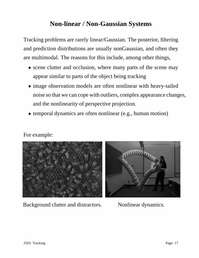
Non-linear / Non-Gaussian Systems

Tracking problems are rarely linear/Gaussian. The posterior, filtering

and prediction distributions are usually nonGaussian, andoften they

are multimodal. The reasons for this include, among other things,

• scene clutter and occlusion, where many parts of the scene may

appear similar to parts of the object being tracking

• image observation models are often nonlinear with heavy-tailed

noise so that we can cope with outliers, complex appearance changes,

and the nonlinearity of perspective projection.

• temporal dynamics are often nonlinear (e.g., human motion)

For example:

Background clutter and distractors. Nonlinear dynamics.


Extended and Unscented Kalman Filters

Extended Kalman Filter (EKF): For nonlinear dynamical models one can linearize the dynamics

at current state; that is,

~xt = f(~xt−1) + ~ηd ≈ A~xt−1 + ~ηd ,

where A = ∇f(~x) |~x=~xt−1and ~ηd ∼ N (0, Cd). One can also iterate the approximation to obtain

the Iterated Extended Kalman Filter (IEKF). In practice the EKF and IEKF have problems unless

the dynamics are close to linear.

Unscented Kalman Filter (UKF): Estimate posterior mean and variance to second-order with ar-

bitrary dynamics[Julier & Uhlmann, 2004]. Rather than linearize the dynamics to ensure Gaussian

predictions, use exact1st and2nd moments of the prediction density under the nonlinear dynamics:

• Choosesigma pointsxj whose sample mean and covariance equal the mean and varianceof

the Gaussian posterior att

• Apply nonlinear dynamics to each sigma point,yj = f(xj), and then compute the sample

mean and covariances of theyj.

Monte Carlosampling

Linear Approx(EKF)

UnscentedTransform


Hill-Climbing

Rather than approximating the posterior or filtering distributions (fully),

just find local maxima of the filtering distribution at each time step.

By also computing the curvature of the log filtering distribution at the

maxima, one obtains local Gaussian approximations.

E.g., Eigen-Tracking[Black & Jepson, ’96]:

• Assume we have learned (offline) a subspace appearance model

for an object under varying pose, articulation, and lighting:

B(x, c) =∑

k

ck Bk(x)

• During tracking, we seek the image warp parametersat, at each

time t, and the subspace coefficientsct such that the warped im-

age isexplainedby the subspace; i.e.,

I(w(x, at), t) ≈ B(x, ct)

• A robust objective function helps cope with modeling errors, oc-

clusions and other outliers:

E(at, ct) =∑

xρ( I(w(x, at), t) − B(x, ct) )

• Initialize the estimation at timet with ML estimate from timet−1.


Eigen-Tracking

Image sequence

Reconstruct

Warp

eigen-images

trainingimages

Training

Test Results:

Figures show superimposed tracking region (top), the best reconstructed

pose (bottom left), and the closest training image (bottom right).


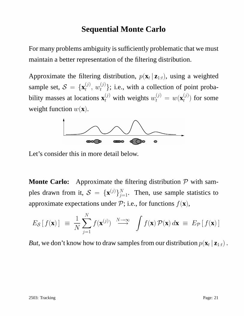
Sequential Monte Carlo

For many problems ambiguity is sufficiently problematic that we must

maintain a better representation of the filtering distribution.

Approximate the filtering distribution,p(xt | z1:t), using a weighted

sample set,S = {x(j)t , w

(j)t }; i.e., with a collection of point proba-

bility masses at locationsx(j)t with weightsw

(j)t = w(x(j)

t ) for some

weight functionw(x).

Let’s consider this in more detail below.

Monte Carlo: Approximate the filtering distributionP with sam-

ples drawn from it,S = {x(j)}Nj=1. Then, use sample statistics to

approximate expectations underP ; i.e., for functionsf(x),

ES [ f(x) ] ≡1

N

N∑

j=1

f(x(j))N→∞−→

∫

f(x)P(x) dx ≡ EP [ f(x) ]

But, we don’t know how to draw samples from our distributionp(xt | z1:t) .


Particle Filter

Importance Sampling: If one draws samplesx(j) from aproposal

distribution, Q(x), with weightsw(j), then

ES [ f(x) ] ≡N∑

j=1

w(j)f(x(j))N→∞−→ EQ [ w(x) f(x) ]

If w(x) = P(x)/Q(x), then the weighted sample statistics approxi-

mate the desired expectations underP(x); i.e.,

EQ [ w(x) f(x) ] =

∫

w(x) f(x)Q(x) dx

=

∫

f(x)P(x) dx

= EP [ f(x) ]

Sequential Monte Carlo [Arulampalam et al, 2002]: The sample

set is updated each time instant, incorporating new data, and possibly

re-sampling the set of state samplesx(j). Key idea: exploit the form

of the filtering distribution for importance sampling,

p(xt | z1:t) = c p(zt | xt) p(xt | z1:t−1)

and the facts that it is often easy to evaluate the likelihood, and one

can usually draw samples from the prediction distribution

Simple Particle Filter: If we sample from the prediction distribution

Q = p(xt | z1:t−1)

then the weights must bew(x) = c p(zt | xt), with c = 1/p(zt | z1:t−1).2503: Tracking Page: 22

Simple Particle Filter

Step 1:Sample the approximate filtering distribution,p(xt−1 | z1:t−1),

given the weighted sample setSt−1 = {x(j)t−1, w

(j)t−1}. To do this, treat

theN weights as probabilities and sample from the cumulative weight

distribution; i.e., draw sampleu ∼ U(0, 1) to sample an indexi.

N

1

00

i

u

Step 2: With samplex(i)t−1, the dynamics provides a distribution over

states at timet, i.e., p(xt | x(i)t−1). A fair sample from the dynamics,

x(j)t ∼ p(xt | x

(i)t−1)

is then a fair sample from the prediction distributionp(xt | z1:t−1).

Step 3:To complete one iteration to find the new filtering distribution,

given the samplesx(j)t , we compute the weightsw(j)

t = c p(zt | x(j)t ):

• p(zt | x(j)t ) is the data likelihood that we know how to evaluate.

• Using Bayes’ rule one can show thatc satisfies

1

c= p(zt | z1:t−1) =

∫

p(zt | xt) p(xt | z1:t−1) dxt ≈∑

j

p(zt | x(j)t )

Using the approximation, the weights become normalized likelihoods

(so they sum to 1).


Particle Filter Remarks

One can think of a sampled approximation as a sum of Dirac delta functions. A weighted sample set

St−1 = {x(j)t−1, w

(j)t−1}, is just a weighted set of delta functions::

p(xt−1 | z1:t−1) =

N∑

j=1

w(j) δ(xt−1 − x(j)t−1)

Sometimes people smooth the delta functions to create smoothed approximations (called Parzen

window density estimates).

If one considers the prediction distribution, and uses the properties of delta functions under inte-

gration, then one obtains a mixture model for the predictiondistribution. That is, given a weighted

sample setSt−1 as above the prediction distribution in (8) is a linear mixture model

p(xt | z1:t−1) =

N∑

j=1

w(j) p(xt | x(j)t−1)

The sampling method on the previous page is just a fair sampling method for linear mixture models.

For more background on particle filters see papers by Gordon et al (1998), Isard and Blake (IJCV,

1998), and by Fearnhead (Phd) and Liu and Chen (JASA, 1998).


Particle Filter Steps

Summary of main steps in basic particle filter:

sample sample normalize

p(xt−1 | z1:t−1) −→ p(xt | xt−1) −→ p(zt | xt) −→ p(xt | z1:t)

filtering temporal likelihood filteringdistribution dynamics evaluation distribution

Depiction of the particle filter process (after[Isard and Blake, ’98]):

weightedsample set

re-sampleand drift

diffuse andre-sample

computelikelihoods

weightedsample set


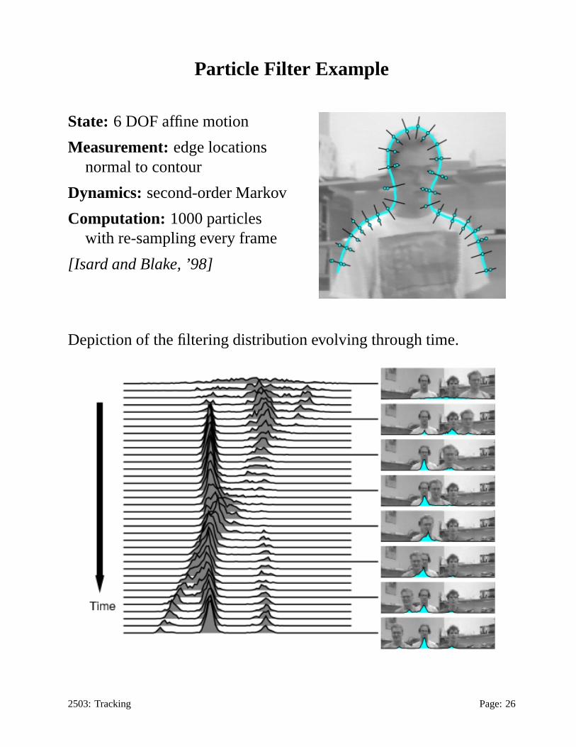
Particle Filter Example

State: 6 DOF affine motion

Measurement:edge locationsnormal to contour

Dynamics: second-order Markov

Computation: 1000 particleswith re-sampling every frame

[Isard and Blake, ’98]

Depiction of the filtering distribution evolving through time.


Particle Explosion in High Dimensions

The number of samplesN required by our simple particle filter de-

pends on the effective volumes (entropies) of the prediction and pos-

terior distributions.

With random sampling from the prediction density,N must grow ex-

ponentially in state dimensionD if we expect enough samples to fall

on states with high posterior probability.

Prediction

Posterior

Prediction

Posterior

E.g., forD-dimensional spheres, with radiiR andr, N ≫(

Rr

)D


Example: 3D People Tracking

Goal: Estimate human pose and

motion from monocular video.

Model State:3D kinematic tree

with 6 global degrees of freedom

and 22 joint angles

top ofhead

rightelbow

rightear

left earrightshoulder

upperback

leftshoulder

leftelbow

lefthand

righthand

lefthip

righthip

lowerback

rightknee

leftkneeright

heel

leftheelLikelihood & Dynamics:

Given the state,s, and camera model, 3D marker positionsXj project

onto the 2D image plane to locations

dj(s) = T (Xj; s) .

Observation model:

d̂j = dj + ηj , ηj ∼ N (0, σ2mI2) .

Likelihood of observed 2D locations,D = {d̂j}:

p(D | s) ∝ exp(−1

2σ2m

∑

j

|| d̂j − dj(s) ||2) .

Smooth dynamics:

st = st−1 + ǫt .

whereǫt is isotropic Gaussian for translational and angular variables.


Example: 3D People Tracking (cont)

Estimator Variance:expected squared error (from posterior mean),

computed over multiple runs with independent noise. WithN fair

posterior samples the estimator variance will decrease like1/N .

105

106

107

10−5

10−4

10−3

10−2

10−1

Computation Time (particle filter samples)

Var

[ mea

n rig

ht h

ip, β

]Hybrid Monte CarloParticle Filter

Full Body Tracker(right hip)

The estimator variance does not decrease anything like1/N . Better

samplers are necessary.

E.g.,Hybrid Monte Carlo Filter [Choo & Fleet 01]: A particle filter

with Markov chain Monte Carlo updates is more efficient.

Particle Filter HMC Filter(black: ground truth; red: mean states from 6 trials)


Effective Sample Size

If we drewN fair samples from the posterior, thenestimator variance

decreases like1/N .

We can approximate the number of “independent” samples (called the

effective sample size) as follows:

Ne ≈1

∑

j(w(j))2

In the worst case, when only one weight is significantly non-zero,Ne

is close to one. In the best case, withN fair samples, all weights are

1/N soNe =N .

In practice,

• when Ne is large (e.g.,> 100, but this depends on the task),

one should not necessarily re-sample the posterior. You mayjust

propagate each sample forward by sampling from the transition

density.

• whenNe is small (e.g.,< 10), you likely have an unreliable pos-

terior approximation, and you may lose track of the target. You

need more or better samples!


Residual Sampling

GivenN samples{xk}Nk=1 with weights{wk}N

k=1, where∑

k wk = 1, and assume that we wish to

drawN new samples (with replacement).

Rather than treating the weights are probabilities of a multinomial distribution and drawingN inde-

pendent samples, one can greatly reduce sampling variability by usingresidual sampling.

• The expected number of times we expect to drawxk is nk = Nwk.

• So first place⌊nk⌋ copies ofxk in the new sample set, and let theresidual weightsbeak =

nk − ⌊nk⌋.

• Then, drawN −∑

k⌊nk⌋ samples (with replacement) according to the probabilitiespk =

ak/∑

k ak.


Use the Current Observation to Improve Proposals

The proposal distributionQ should be as close as possible to the filtering distributionP that we wish

to approximate. Otherwise,

• many particles will have weights near zero, contributing very little to the approximation to the

filtering disitribution;

• we may even fail to sample significant regions of the state space, so the normalization constant

c can be wildly wrong.

For visual tracking, the prediction distributionQ = p(xt | z1:t−1) often yields very poor proposals,

because dynamics are often very uncertain, and likelihoodsare often very peaked by comparison.

One way to greatly improve proposals is to use the current observation. For example, imagine that

you are tracking faces and you have a low-level face detector.

• LetD(xt) be a continuous distribution obtained from some low-level detector which indicates

where faces might be (e.g., Gaussian modes at locations of classifier hits).

• Then, just modify the proposal density and importance weights:

Q(xt) = D(xt) p(xt | z1:t−1) , with w(xt) =c p(zt | xt)

D(xt)


Explain All Observations

Don’t compare different states based on different sets of observations.

• If one hypothesizes two target locations,s1 ands2, and extracts target-sized image regions

centered at both locations,I1 andI2, it makes no sense to says1 is more likely if p(I1 | s1) >

p(I2 | s2).

• Rather, usep(I | s1) andp(I | s2) whereI is the entire image.

Explain the entire image, or use likelihood ratios (for efficiency).

E.g., assume that pixelsI(y), given the state, are independent, so

p(I | x) =∏

y∈Df

pf (I(y) | s)∏

y∈Db

pb(I(y))

whereDf and Db are disjoint sets of foreground and background pixels, andpf and pb are the

respective likelihood functions.

Divide p(I | s) by the background likelihood of all pixels (i.e., as if no target is present):

p(I | s) ∝

∏

y∈Dfpf(I(y) | s)

∏

y∈Dbpb(I(y))

∏

ypb(I(y))

=

∏

y∈Dfpf(I(y) | s)

∏

y∈Dbpb(I(y))

∏

y∈Dfpb(I(y) | s)

∏

y∈Dbpb(I(y))

=∏

y∈Df

pf(I(y) | x)

pb(I(y))


Conditional Observation Independence

What about independence of measurements?

Pixels have correlated (dependent) noise because of several factors:

• models are wrong (most noise is model error)

• failures in feature tracking are not independent for different features.

• overlapping windows are often used to extract measurements

Consequence: Likelihood functions are often more sharply peaked than they ought to be.


Summary and Further Remarks on Filtering

• posteriors must be sufficiently constrained, with some combina-

tions of posterior factorization, dynamics, measurements, ..

• proposal distributions should be non-zero wherever the posterior

distribution is non-zero (usually heavy-tailed)

• proposals should exploit current observations in additionto pre-

diction distribution

• likelihoods should be compared against the same observations

• sampling variability can be a problem

– must have enough samples in regions of high probability for

normalization to be useful

– too many samples needed for high dimensional problems (esp.

when samples drawn independently from prediction dist)

– samples tend to migrate to a single mode (don’t design a par-

ticle filter to track multiple objects with a state that represents

only one such object)

– sample deterministically where possible

– exploit diagnostics to monitor effective numbers of samples


Further Readings

Arulampalam, M.S., Maskell, S., Gordon, N. and Clapp, T. (2002) A tutorial on particle filters for

online nonlinear/non-Gaussian Bayesian tracking.IEEE Trans. Signal Proc.50(2):174–188

Black, M.J. and Jepson, A.D. (1996) Eigentracking: Robust matching and tracking of articulated

objects using a view-based representation.Int. J. Computer Vision, 26:63–84.

Blake, A. (2005) Visual tracking. InMathematical models for Computer Vision: The Handbook.

N. Paragios, Y. Chen, and O. Faugeras (eds.), Springer, 2005.

Carpenter, Clifford and Fearnhead (1999) An improved particle filter for nonlinear problems. IEE

Proc. Radar Sonar Navig., 146(1)

Doucet, A., Godsill, S., and Andrieu, C. (2000) On sequential Monte Carlo sampling methods for

Bayesian filtering.Stats and Computing, 10:197–208.

Gordon, N.J., Salmond, D.J. and Smith, A.F.M. (1993) Novel approach to nonlinear/non-Gaussian

Bayesian state estimation.IEE Proceedings-F, 140(2):107–113.

Isard, M. and Blake, A. (1998) Condensation: Conditional density propagation.Int. J. Computer

Vision, 29(1):2–28.

Jepson, A.D., Fleet, D.J. and El-Maraghi, T. (2003) Robust,on-line appearance models for visual

tracking.IEEE Trans. on PAMI, 25(10):1296–1311

Julier, S.J. and Uhlmann, J.K. (2004) Unscented filtering and nonlinear estimation.Proceedings

of the IEEE, 92(3):401–422

Khan, Z., Balch, T. and Dellaert, F. (2004) A Rao-Blackwellized particle filter for EigenTracking.

Proc. IEEE CVPR.

Sidenbladh, H., Black, M.J. and Fleet, D.J. (2000) Stochastic tracking of 3D human figures using

2D image motion.Proc. ECCV, pp. 702–718, Dublin, Springer.

Wan, E.A. and van der Merwe, R. (2000) The unscented Kalman filter for nonlinear estimation.

(see van der Merwe’s web site for the TR)


tracking - university of torontojepson/csc2503/tracking.pdf · tracking goal: fundamentals of...

Documents