TRACTION ESTIMATION AND CONTROL FOR MOBILE ROBOTS

by Jared D. Terry A thesis submitted to the faculty of The University of Utah in partial fulfillment of the requirements for the degree of Master of Science Department of Mechanical Engineering University of Utah May 2007

Copyright © Jared D. Terry 2007

All Rights Reserved

T H E U N I V E R S I T Y O F U T A H G R A D U A T E S C H O O L

SUPERVISORY COMMITTEE APPROVAL

of a thesis submitted by

This thesis has been read by each member of the following supervisory committee and by majority vote has been found to be satisfactory. __________________ _________________________________________

Chair: __________________ _________________________________________ __________________ _________________________________________

T H E U N I V E R S I T Y O F U T A H G R A D U A T E S C H O O L

F I N A L R E A D I N G A P P R O V A L

To the Graduate Council of the University of Utah: I have read the thesis of in its final form and have found that (1) its format, citations, and bibliographic style are consistent and acceptable; (2) its illustrative materials including figures, tables, and charts are in place; and (3) the final manuscript is satisfactory to the supervisory committee and is ready for submission to The Graduate School. ________________________ ______________________________________

Date Chair: Supervisory Committee

Approved for the Major Department

_____________________________________

Chair/Dean

Approved for the Graduate Council

_____________________________________ David S. Chapman

Dean of The Graduate School

i

ABSTRACT

Mobile Robots are used to venture through types of environments where wheel

slip is a threat. Wheel slip is a hazard to mobile robots in that it introduces error in dead

reckoning measurement and in some instances causes the robot to halt is forward

progress. To compensate for traction loss several methods are used to determine the

terrain characteristics. One of these methods is Pacejka’s Tire Model. The slope of

Pacejka’s Tire Model can be used to determine when traction loss occurs.

One step toward realizing the slope of Pacejka’s Tire Model is achieving a good

estimate of wheel slip. We present a unique traction estimation algorithm that estimates

traction loss by measuring the wheel slip velocity and its derivative. Our algorithm

estimates the wheel slip velocity and its derivative by coupling the dynamics of a wheel

with the dynamics of a vehicle. Estimates of the wheel slip velocity and its derivative are

accomplished using onboard sensors. To obtain an accurate estimate of the wheel slip

velocity and its derivative, we propose a modified Kalman Filter that fuses a system

model of a DC motor with an estimate of the disturbances acting on the system model.

Using the wheel slip velocity and its derivative a neighborhood can be defined between

two instances in time that estimates when traction loss occurring.

ii With means of estimating traction loss, we propose a traction control law that

provides the ability of tracking a desired reference while mitigating traction loss. To

solve the tracking problem we propose a robust tracking controller that provides the

ability of following a defined path and rejecting unmodled disturbance. To mitigate

traction loss we propose a continuous robust traction controller to maximize traction

forces by containing wheel slip and its derivative to a neighborhood. The unique aspect

of our traction controller is it works jointly with our proposed tracking controller.

iii

TABLE OF CONTENTS

ABSTRACT..............................................................................................................I

TABLE OF CONTENTS.........................................................................................III

LIST OF TABLES................................................................................................... V

LIST OF FIGURES ................................................................................................ VI

ACKNOWLEDGEMENTS................................................................................... VIII

1. INTRODUCTION ..............................................................................................1

1.1. Pacejka’s Tire Model .................................................................................3 1.2. Background................................................................................................7 1.3. Contributions.............................................................................................10 1.4. Thesis Structure ........................................................................................13

2. TRACTION ESTIMATION FOR A MOBILE ROBOT ..................................14

2.1. Introduction...............................................................................................14 2.2. Overall Traction Estimation Algorithm....................................................16 2.3. Traction Estimation: Wheel Slip Estimation ............................................17 2.4. Kalman Filter Design................................................................................20

2.4.1. General Kalman Filter Design ......................................................20 2.4.2. Modified Kalman Filter Design ....................................................22

2.5. Output Feedback Control..........................................................................26 2.6. Experimental Results ................................................................................29

2.6.1. Methods and Procedures ...............................................................29 2.6.2. Results and Discussion .................................................................32

3. TRACTION CONTROL OF A MOBILE ROBOT...........................................38

3.1. Introduction...............................................................................................38 3.2. Traction Control Design ...........................................................................41

iv 3.2.1. Robust Tracking Control Design ..................................................41 3.2.2. Traction Control Design ...............................................................45

3.3. Experimental Evaluation...........................................................................51

3.3.1. Methods and Procedures ...............................................................51 3.3.2. Experimental Results and Discussion...........................................54

4. CONCLUSION AND FUTURE WORK ..........................................................59

4.1. Traction Estimation...................................................................................59 4.2. Traction Control........................................................................................62

APPENDIX..............................................................................................................64

REFERENCES ........................................................................................................67

v

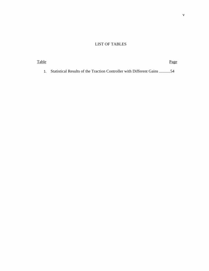
LIST OF TABLES

Table Page

1. Statistical Results of the Traction Controller with Different Gains ...........54

vi

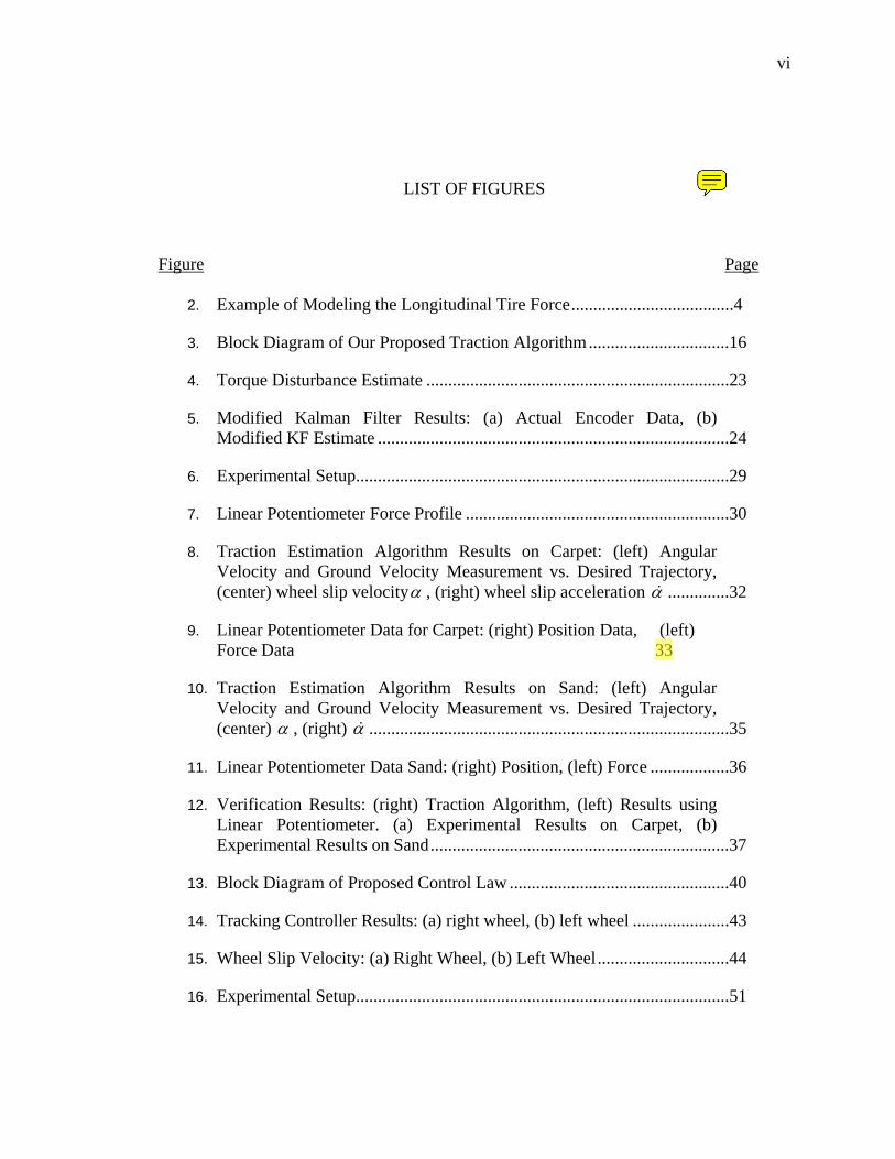
LIST OF FIGURES

Figure Page

2. Example of Modeling the Longitudinal Tire Force.....................................4

3. Block Diagram of Our Proposed Traction Algorithm................................16

4. Torque Disturbance Estimate .....................................................................23

5. Modified Kalman Filter Results: (a) Actual Encoder Data, (b) Modified KF Estimate ................................................................................24

6. Experimental Setup.....................................................................................29

7. Linear Potentiometer Force Profile ............................................................30

8. Traction Estimation Algorithm Results on Carpet: (left) Angular Velocity and Ground Velocity Measurement vs. Desired Trajectory, (center) wheel slip velocityα , (right) wheel slip acceleration α ..............32

9. Linear Potentiometer Data for Carpet: (right) Position Data, (left) Force Data 33

10. Traction Estimation Algorithm Results on Sand: (left) Angular Velocity and Ground Velocity Measurement vs. Desired Trajectory, (center) α , (right) α ..................................................................................35

11. Linear Potentiometer Data Sand: (right) Position, (left) Force ..................36

12. Verification Results: (right) Traction Algorithm, (left) Results using Linear Potentiometer. (a) Experimental Results on Carpet, (b) Experimental Results on Sand....................................................................37

13. Block Diagram of Proposed Control Law ..................................................40

14. Tracking Controller Results: (a) right wheel, (b) left wheel ......................43

15. Wheel Slip Velocity: (a) Right Wheel, (b) Left Wheel..............................44

16. Experimental Setup.....................................................................................51

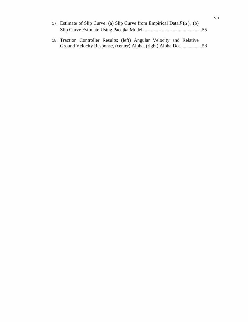
vii 17. Estimate of Slip Curve: (a) Slip Curve from Empirical Data ( )F α , (b)

Slip Curve Estimate Using Pacejka Model.................................................55

18. Traction Controller Results: (left) Angular Velocity and Relative Ground Velocity Response, (center) Alpha, (right) Alpha Dot..................58

viii

ACKNOWLEDGEMENTS

I would like to thank Dr. Mark A. Minor for his guidance and leadership, Jill Terry

for her love and support, and Karen Hayes and Courtney Terry for assisting me in proof

reading my Thesis.

1

1. INTRODUCTION

Planetary rovers and other robots have been designed to travel in environments

where the risk to human safety is high. The majority of these environments, ill suited for

human exploration, are rough, difficult terrain. Some of these environments may be a

disaster site, a mining tunnel, or the surface of Mars.

To transverse through these types of environments, robots have been designed with

specific types of modality. [1] proposed a spherical robot design capable of rolling

motion, while [2] proposed a control design for a two axel, compliant frame, mobile

robot. [3] and [4] proposed walking robots. Both [1] and [2] simplify their kinematic

model by assuming the robot is under the constraint of pure rolling without slip. This

assumption, however, does not accurately model the interaction between of the terrain of

the environment and the rolling surface. For mobile robots an accurate model describing

the interaction between the wheels and the terrain require an estimate of wheel slip.

Wheel slip will cause error in dead reckoning measurement in mobile robots. The

mobile robot, therefore, will assume its posture and position are different from what they

actually are. Wheel slip may also cause the mobile robot to dig into the terrain and stop

its forward momentum. To maximize the ability of mobile robots to transverse over

difficult terrain where wheel slip is a potential threat, the mobile robot must be infused

2

with a method to estimate traction loss and use that method to mitigate traction loss

through a traction controller.

We propose a method based upon a data fusion algorithm that provides an estimate

of traction loss. The underlying foundation of our traction estimation algorithm is based

upon the derivative of Pacejka’s Tire Model [5]. The derivative of this tire model can be

used to define regions where traction is available or being lost. Our method, however,

does not provide the ability, at this time, of estimating the derivative of Pacejka’s Tire

Model but provides an estimate of the wheel slip velocity and its derivative. Having an

estimate of the wheel slip velocity is a necessary evolutionary step towards having the

ability of estimating the derivative of the slip curve. Using an estimate of the wheel slip

velocity and its derivative, a neighborhood can be defined where traction loss is

occurring. Validation of our traction estimation algorithm is provided through

experimental results. Experiments were conducted on multiple surfaces and a discussion

outlining the performance of our traction estimation algorithm will be given.

Applying our traction estimation algorithm, we also propose a traction control law

which provides means of tracking a reference velocity while mitigating traction loss. Our

control law was designed to enable a desired reference to be tracked when traction loss is

not occurring. To mitigate traction loss we provide a continuous robust controller that

maximizes traction by riding the peak of the slip curve. Our proposed traction control law

also confines the traction estimation variables to a defined neighborhood. To determine

our control gains to maximize traction, multiple tests were conducted on a predetermined

surface.

3

1.1. Pacejka’s Tire Model

To provide mobile robots the capability of estimating when traction loss occurs, a

model describing the interaction between traction forces and a rolling surface must be

acquired. [5] determined an empirical tire model describing the interaction between

vehicle dynamics and tire forces. This tire model is known as the Pacejka’s Tire Model.

The model utilizes several variables for estimating traction forces. Assuming the only

required parameters are the normal force, the terrain characteristics, and the vehicle

dynamics, this tire model is reduced to

( ) ( ( ))F t f tλ= , (1)

where ( )F t denotes the longitudinal friction force and λ is the slip ratio. The slip ratio

can be defined as

( )( ) 1 ,0 1( )

v ttt r

λ λω

= − ≤ ≤ , (2)

where v is the linear velocity of a vehicle, ω is the angular velocity of a tire, r is the

radius of the tire, and /v r is defined as the relative ground velocity

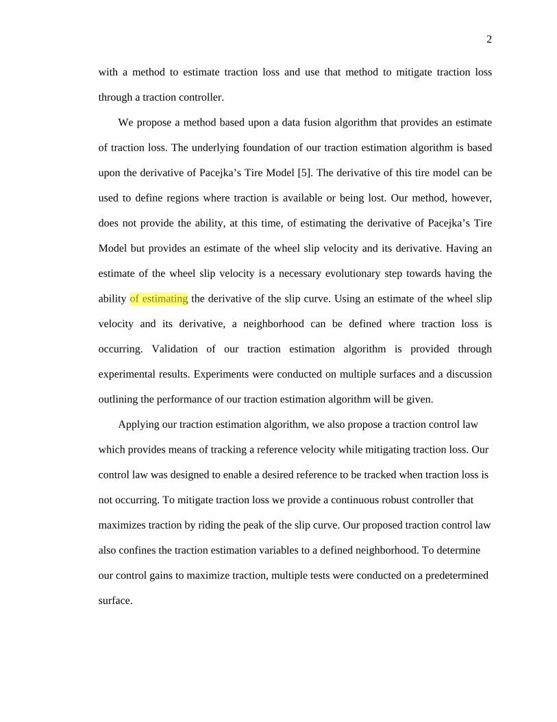
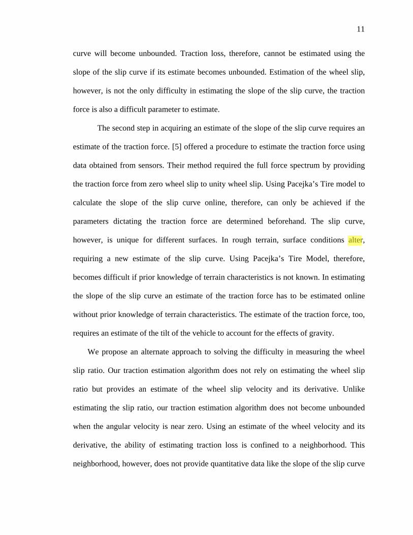
Fig. 1 is an example of implementing (1), which provides an estimate of the

friction coefficient, µ , as a function of the slip ratio, λ . The friction coefficient was

chosen to be the output variable due to its independence from the normal force. Upon

inspection of Fig. 1, certain causal relationships can be developed which build the

foundation for the proposed traction estimation algorithm.

4

The first causal relationship is when 0λ ≡ . At this point the relative ground

velocity of the vehicle matches that of the angular velocity of the wheel. This

corresponds to the ideal kinematic of pure rolling without slip. The traction force at this

point is zero.

The second causal relationship is defined in a region 2D R⊂

where 2max max{ , | 0 ,0 }D Rµ λ µ µ λ λ= ∈ < < < < . In this region the friction coefficient, µ ,

and the slip ratio, λ , are monotonically increasing. Since the friction coefficient

correlates to the longitudinal traction force, this shows that in region D there is traction

available to accelerate a vehicle.

The third causal relationship is defined in region 2G R⊂ ,

where 2max max{ , | , 1}fG Rµ λ µ µ µ λ λ= ∈ < ≤ < ≤ . In this region, µ is monotonically

decreasing while λ is monotonically increasing. Since the traction force is decreasing, the

angular velocity of the vehicle will continue increasing while the relative ground velocity

will decrease. When the slip ratio equates to one the system is in pure slip meaning the

angular velocity of the wheel is spinning and the relative ground velocity is zero.

Figure: 1 Example of Modeling the Longitudinal Tire Force

5

The fourth causal relationship occurs at the point maxµ µ≡ and maxλ λ≡ . At this

point traction has reached a maximum. Any further increase in slip will drive the system

into region G and cause traction loss to occur. If slip decreases, the system will be driven

into region D where traction is available.

Assuming the friction coefficient, µ , and the slip ratio, λ , are sensible parameters,

a heuristic can be derived that will ensure traction will be contained in region D. This

heuristic can be derived through inspection of the slip curve. Knowing the derivatives of

µ and λ are monotonically increasing in region D the derivative of the slip curve is

defined as

( ) ( ) ( )sin( ) sin( ) 0 ,( ) ( ) ( )

dF t d t tmg mg Dd t d t t

µ µθ θ µ λλ λ λ

= = > ∀ ∈ , (3)

where m is the mass of the vehicle supported by the wheel and sin( )g θ is the angular

component of gravity. In region D traction loss is not occurring since the derivative of the

slip curve is positive. In region G, however, the derivative of the slip curve is negative,

delineating that traction loss. The derivative of the slip curve in region G, therefore, is

monotonically decreasing,

sin( ) 0, ,dmg Gd

µθ µ λλ

< ∀ ∈ . (4)

By measuring the friction coefficient and the slip ratio, the derivative of the slip curve

can be calculated. To maximize traction, the derivative of the slip curve should be

contained near the peak of the slip curve. If the derivative, therefore, is contained in D,

6

the system should be driven within some small boundary of the peak of the slip curve. If

by causality the derivative is negative, the system should be driven into region D.

7

1.2. Background

Using mobile robots in different terrain has been an area of interest for many

researchers. Each offers their preferred method of estimating terrain characteristics and a

solution to overcoming the problems of traction loss. [6] expressed their interests in

planetary expeditions using mobile robots. They argued that mobile robots require the

ability of navigating through rough terrain. To navigate through rough terrain they argue

a mobile robot requires a means of estimating terrain characteristics. [7] argued that using

odometry to track the relative position of a mobile robot on these surfaces is not useful.

[2] performed tests with their mobile robot on rough terrain environments and concluded

that their tracking error was due to their sensing system, rather than their dynamic

controller. On the experimental surfaces, their sensing system error was propagated by

wheel slip. To decrease the effects of sensory error due to traction loss, wheel slip must

be considered in the control of exploratory robots.

Using Pacejka’s Tire Model, however, is not the only method of estimating traction

loss. [8]and [7] proposed that estimation of traction loss on soft surfaces was achievable

by determining the shear stress between the wheel and the surface using the Columb-

Morh soil failure criteria. Like Pacejka, they utilized an estimate of wheel slip to create a

model to determine when traction loss was occurring. Both [8] and [7] proposed

architecture to estimate traction loss could be implemented on predefined surfaces or on

surfaces where terrain characteristics were unknown. If terrain characteristics were not

available, least squares regression was used to determine its characteristics. [7] offered a

solution to correct odometry error due to wheel slip. No traction controller was provided.

8

[8], however, did provide control and optimization techniques, but no control law or

stability proof was provided.

[8] and [7] proposed architecture was based upon least squares regression to estimate

terrain characteristics. Founding their terrain estimation technique on least squares

regression requires a certain number of poses from sensory data to obtain good parameter

estimation. [9], [10], and [11] all proposed solutions to determine the number of poses

required for good observability for parameter estimation. Since [6] and [7] proposed a

least squares regression for determining terrain characteristics, there will be a delay in

parameter estimation. This delay induces error into their traction loss detection algorithm.

[7] concluded that their traction estimation algorithm took time to converge to an

accurate solution for wheel slip, but they never gave the time delay.

The Dugoff Tire Model is another model used to predict traction loss [12]. Using this

model for ABS braking, [13], [14], and [15] introduced a sliding mode controller that

would drive wheel slip to a desired reference while braking. Recognizing the difficulty in

measuring the linear velocity of the vehicle, [15] proposed a sliding mode observed to

acquire a better estimate of linear velocity. Their observer, however, required prior

knowledge of terrain characteristics. They did not introduce a method to estimate the

terrain characteristics online like [8] and [7]. [13] mentioned the estimation of the terrain

characteristics could be determined from sensors and an observer, but no observer design

was derived.

9

[16] used a different tire model and proposed a dynamic feedback controller to

compensate for traction loss. The controller was designed using linearization, and the

author provided no simulation on parameter uncertainty or unmodled disturbances to test

the region of stability for their control law.

Neither [8], [7], [13], [14], [15], or [16] attempted to solve the wheel tracking

problem with their control design. Their methods only introduced a controller to account

for wheel slip. [17], however, introduced a Backstepping controller capable of solving the

tracking problem while compensating for traction loss. Their controller simplified the

Tire model by assuming slip was contained to a linear estimate of the slip curve. Using

this estimate they proposed a Backstepping controller that would drive the velocity of a

vehicle to a desired reference while compensating for wheel slip. Their Backstepping

control law, however, was founded on the inverse of the angular velocity. Their control

design was able to produce repeatable results in simulation, but no results pertaining to

the actual angular velocity nor the susceptibility of their control law becoming

unbounded when the angular velocity approached zero was discussed. Neither was their

control law used on an actual system for experimentation.

10

1.3. Contributions

To estimate traction loss, our goal is to estimate the slope of the slip curve by

using onboard sensors to estimate when traction loss is occurring. Using the slope of the

slip curve a control law can be derived to maximize traction forces. To achieve this goal

several steps must be overcome. The first step is estimating the slip ratio. Measuring the

slip ratio has inherent difficulties. The slip ratio (2) is discontinuous at 0ω ≈ . The

assumed bound on the slip ratio, therefore, becomes invalid. Estimating the wheel slip,

therefore, can only be achieved if the wheel is spinning.

In the derivation of their sliding mode control design for ABS braking [13], [14],

and [15] never discussed the threat of wheel slip becoming unbounded. In their

simulations the angular velocity and linear velocity are kept well above zero.

Another difficulty with estimating the wheel slip is providing an accurate method

of measuring signals from sensors. Using accelerometer signals to estimate the vehicle

dynamics are prone to vibration and bias drift. Using encoder signals to estimate wheel

odometry are noisy due to the measurement being discrete. To provide meaningful

estimates of wheel velocity and linear velocity, the signals have to be filtered using

Kalman Filters of Observers to ascertain a good measurement of wheel slip.

Using an accurate estimate of wheel slip, however, can still cause difficulty in

estimating the slope of the slip curve. To achieve an estimate of the slip curve, the

derivative of the wheel slip has to be acquired. Implementing controllers that drive the

wheel slip to a desired reference, similar to [13], [14], and [15], will result in the

derivative of the wheel slip to become zero and the estimation of the slope of the slip

11

curve will become unbounded. Traction loss, therefore, cannot be estimated using the

slope of the slip curve if its estimate becomes unbounded. Estimation of the wheel slip,

however, is not the only difficulty in estimating the slope of the slip curve, the traction

force is also a difficult parameter to estimate.

The second step in acquiring an estimate of the slope of the slip curve requires an

estimate of the traction force. [5] offered a procedure to estimate the traction force using

data obtained from sensors. Their method required the full force spectrum by providing

the traction force from zero wheel slip to unity wheel slip. Using Pacejka’s Tire model to

calculate the slope of the slip curve online, therefore, can only be achieved if the

parameters dictating the traction force are determined beforehand. The slip curve,

however, is unique for different surfaces. In rough terrain, surface conditions alter,

requiring a new estimate of the slip curve. Using Pacejka’s Tire Model, therefore,

becomes difficult if prior knowledge of terrain characteristics is not known. In estimating

the slope of the slip curve an estimate of the traction force has to be estimated online

without prior knowledge of terrain characteristics. The estimate of the traction force, too,

requires an estimate of the tilt of the vehicle to account for the effects of gravity.

We propose an alternate approach to solving the difficulty in measuring the wheel

slip ratio. Our traction estimation algorithm does not rely on estimating the wheel slip

ratio but provides an estimate of the wheel slip velocity and its derivative. Unlike

estimating the slip ratio, our traction estimation algorithm does not become unbounded

when the angular velocity is near zero. Using an estimate of the wheel velocity and its

derivative, the ability of estimating traction loss is confined to a neighborhood. This

neighborhood, however, does not provide quantitative data like the slope of the slip curve

12

but provides qualitative data by defining a boundary, whose limits are two instances in

time, to estimate traction loss. Using this neighborhood to estimate when traction loss is

occurring can be used on both hard and soft terrains. Our traction estimation algorithm

also does not utilize least squares regression to estimate traction loss but only requires an

estimate of the angular and linear velocity. Estimation of the wheel slip velocity is not

prone to a delay like [7] had in estimating wheel slip.

To provide a better estimate of the angular velocity of the wheel, we also propose a

modified Kalman Filter. The unique aspect of our modified Kalman Filter is that the filter

utilizes an estimate of the disturbance torque and an ideal motor model to arrive at a

better estimate of the angular velocity of the wheel. The estimate of the angular velocity

and the estimate of the linear velocity are used to determine the wheel slip velocity and

its derivative.

Using the estimate of wheel slip velocity we propose a traction control law that also

is integrated with a tracking controller. Our traction control law does not attempt to drive

the wheel slip velocity to a desired reference like, [13], [14], and[15] but confines the

wheel slip velocity to a neighborhood. Confining the wheel slip velocity to a

neighborhood provides our control law with the liberty to allow the appropriate

magnitude of wheel slip to track a desired angular velocity reference. If tracking the

desired reference requires more traction than is available on the surface, our control law

confines the wheel slip velocity to a nominal value near the peak of the slip curve. By

using an estimate of the wheel slip velocity, the control input does not suffer from

becoming unbounded like [17] .

13

1.4. Thesis Structure

Chapter 2 outlines our proposed traction estimation algorithm. Our algorithm

foundation is built upon the Pacejka Tire Model. Using this model we couple vehicle

dynamics to deduce our traction estimation algorithm. The benefit of our traction

estimation algorithm is the ability of measuring traction loss through measurement of

vehicle dynamics without prior knowledge of terrain characteristics. Experimentation on

multiple surfaces was explored. Through our results we will validate our algorithm.

Chapter 3 outlines our proposed traction control law which provides means of

tracking a reference velocity while compensating for traction loss. Estimation of traction

loss is obtained through a modified vehicle dynamic equation which we propose in

Chapter 2. The control laws for tracking and traction control will be provided. Stability of

implementing the traction controller in conjunction with the tracking controller will be

proved through a Lyapunov candidate function. Experimental results of our traction

controller will be given and a discussion of the traction controller performance will be

evaluated.

14

2. TRACTION ESTIMATION FOR A MOBILE ROBOT

2.1. Introduction

In this chapter we introduce our proposed traction algorithm. Unlike [8] and [7]

which use shear forces to estimate traction loss, we propose using an alternate

approach. Our traction estimation algorithm models the dynamics of the wheel and

the dynamics of the vehicle by using Pacejka’s Tire model [5]. By coupling the

vehicle dynamics and the Pacejka’s Tire Model our traction estimation algorithm

model provides an estimate of the wheel slip velocity and its derivative through a

first order differential equation. The use of this differential equation, however, is not

necessary since the wheel slip velocity and its derivative can be estimated using

onboard sensors. Encoders measure wheel odometry while an accelerometer

measures the acceleration of the vehicle. To provide a good estimate of the angular

velocity we present a modified Kalman Filter that gives a better estimate of encoder

data. This Kalman Filter is unique in that is fuses encoder data with an estimate of

motor disturbances to arrive at a better estimate of the angular velocity of the wheel.

Using this estimate of the angular velocity of the wheel provides a better estimate of

the wheel slip velocity and its derivative.

15

To validate our traction estimation algorithm we conducted tests on carpet and

sand. To ensure experiments with repeatable wheel slip we designed an output

feedback controller to control wheel speed. Using this control law we provided the

ability of tracking a predetermined, angular velocity, reference. Given this reference

our experiments were able to produce repeatable wheel slip.

Through our results we show our traction estimation algorithm provides the

ability of estimating traction loss. Using the wheel slip velocity and its derivative, a

neighborhood can be defined between two instances in time where traction loss is

occurring. This neighborhood provides a qualitative estimate of traction loss. By

conducting experiments on different surfaces our traction estimation algorithm also

provided the ability of estimating traction loss on hard and soft surfaces.

16

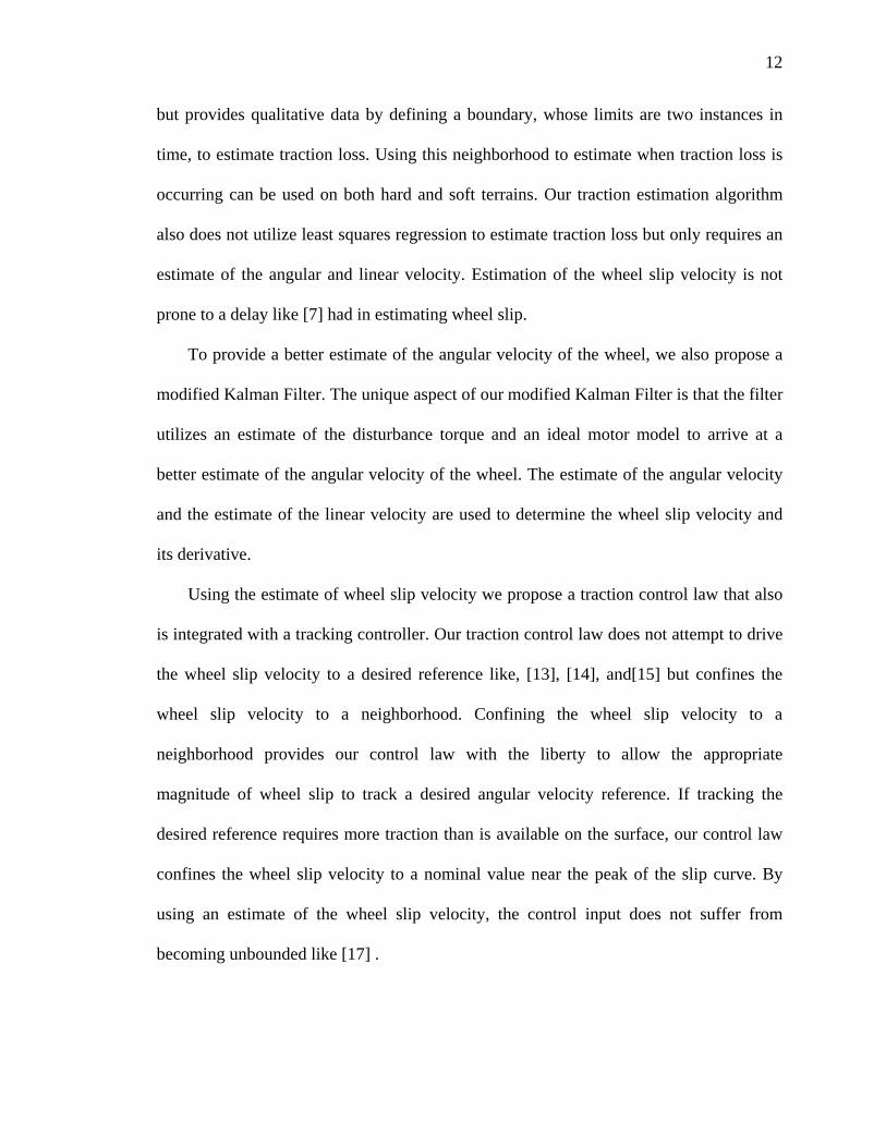
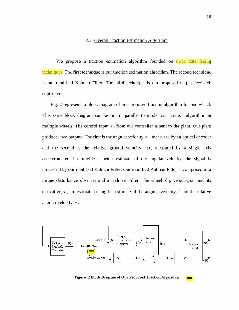
2.2. Overall Traction Estimation Algorithm

We propose a traction estimation algorithm founded on three data fusing

techniques. The first technique is our traction estimation algorithm. The second technique

is our modified Kalman Filter. The third technique is our proposed output feedback

controller.

Fig. 2 represents a block diagram of our proposed traction algorithm for one wheel.

This same block diagram can be run in parallel to model our traction algorithm on

multiple wheels. The control input, u, from our controller is sent to the plant. Our plant

produces two outputs. The first is the angular velocity,ω , measured by an optical encoder

and the second is the relative ground velocity, v/r, measured by a single axis

accelerometer. To provide a better estimate of the angular velocity, the signal is

processed by our modified Kalman Filter. Our modified Kalman Filter is comprised of a

torque disturbance observer and a Kalman Filter. The wheel slip velocity,α , and its

derivative,α , are estimated using the estimate of the angular velocity,ω and the relative

angular velocity, v/r.

Figure: 2 Block Diagram of Our Proposed Traction Algorithm

17

2.3. Traction Estimation: Wheel Slip Estimation

Our object is to determine a method to negate the estimate of the wheel slip ratio, λ ,

but providing an estimate of the wheel slip velocity, α . Providing an estimate of the

wheel speed velocity is the first step towards estimating the derivative of the slip curve.

To derive an estimate of the wheel slip velocity a model must be derived that couples the

dynamics of the wheel with the dynamics of the vehicle.

To accomplish this, assume the dynamics of a vehicle are given as,

ˆmv bv F+ = , (5)

where m and b are estimates of the mass and damping of the physical system and F is

the forcing on the system modeled by (1). Solving (2) for v and v yields,

(1 );

(1 )

v r

v r r

ω λ

ω λ ω λ

= −

= − +. (6)

Substituting (6) into (5) gives,

ˆˆ[ (1 ) ] [ (1 )]m r r b r Fω λ ω λ ω λ− − + − = . (7)

Recognizing the derivative of ωλ which appears in (7) allows the equation to be

rearranged into the form,

ˆ ˆ

ˆ ˆ ˆb b Fm m m

ωλ λω ω ωλ ω+ = − + − . (8)

18

Using the change of variables,

,α ωλ α ωλ ωλ= = + , (9)

and substituting them into (8) provides the equation

ˆ

ˆb um

α α= − + , (10)

where

1 ( )ˆ

u Fm

τ= − . (11)

and

ˆ

ˆ ˆbm m

τω ω+ = . (12)

Providing a change of variables using α and α to simplify (8) resulted in a

simple first order differential equation, (10). The physical interpretation of α and α are

hard to determine by (9) alone. To acquire a better representation of the physical

interpretation of these variables (9) can be reduced by substituting (2) into (9) which

yields

,v vr r

α ω α ω= − = − . (13)

In this form the traction estimation variables [ ]α α are simply the error between the

angular velocity of the wheel, ω , and the relative ground velocity, /v r , and can be

19

measured by onboard sensors. In this form the wheel slip ratio has been transformed into

the wheel slip velocity,α , and its derivative.

Modifying (5) through a change of variables yields (10), which provides an

alternate first order differential equation which estimates the wheel slip velocity, α , and

its derivative. This differential equation is founded upon the causal relationship between

the dynamics of the wheel, (12), and the dynamics of the vehicle, (5). The input of (10)

being zero signifies a perfect mapping between the torque input of the wheel and the

forcing input of the vehicle by (11). When slip occurs the torque input will not map

perfectly to the forcing input. The disturbances of the terrain interacting with the

dynamics of the vehicle, therefore, are coupled into this estimation of α .

The causal relationship provided by (10) only describes the nominal wheel slip

velocity since the nominal linear velocity is provided by only one wheel. This assumption

simplifies the forward motion of the vehicle and is an assumption made by [5]. In reality

the forward velocity of a vehicle is determined by the independent linear velocity of each

wheel. To determine the independent linear velocity of each wheel an estimation of the

traction forces on each wheel is required. The coupling of the independent traction forces

of each wheel to control the forward motion of the mobile robot is the subject of future

research.

20

2.4. Kalman Filter Design

2.4.1. General Kalman Filter Design

To achieve a good estimate of traction loss, our traction estimation algorithm

requires the use of onboard sensors. Wheel odometry measurement is provided by an

optical encoder on each wheel. Vehicle acceleration is measured using a single axis

accelerometer aligned with the forward direction of the robot. To calculate α the angular

acceleration of the wheels has to be derived from encoder data. To reduce sensory noise

from the encoder data we propose implementing a Kalman Filter to acquire a better

estimate of wheel speed and acceleration.

The general state equation representing the dynamics of a wheel takes the general

form with unknown process and output noise,

;

B , , 1, 1ˆ ˆJt

m

x x u wy x v

KR J

= + += +

= − = = =

A B GC

A B C G

(14)

where x represents the angular velocity of a wheel, u is the motor voltage input, and y is

the output of our state model provided through encoder data. B and J are the estimates

of the mechanical damping and the inertia of the wheel. The electrical components of the

armature of the DC motor, tK and mR , are the torque constant of the motor and the

resistance of the armature. The signal w is an unknown process noise acting on the plant

from the voltage input. The signal v is unknown measurement noise from the encoder.

21

We desire to design a Kalman Filter to provide a better estimate of the angular

velocity of the wheel. Assume the observer to estimate the angular velocity is

ˆ ˆ ˆ( )x x u y y= + + −A B L , (15)

where L is the observer gain to provide an optimal estimate of the angular velocity in the

presence of the process noise, w, and the output noise, v. To determine the appropriate

observer gain, the error covariance, P , must be solved using the algebraic Riccati

equation

1 0T T −+ + − =AP PA GQG PCR CP , (16)

Where R is the covariance of the output noise, and T=Q C C . Solving for the error

covariance, P , provides the ability of determining the optimal observer gain, L where

1T −=L PC R (17)

This Kalman Filter design uses the ideal system model of a DC motor to acquire a

better estimate of the angular velocity. The ideal system model of a DC motor, however,

does not account for disturbances acting on the system. An unknown disturbance acting

on the system will cause a larger deviation between the actual angular velocity and the

estimate of the angular velocity. Larger deviations in the measured verses estimated

angular velocity require the optimal observer gain to weigh a higher confidence in the

measured data. Placing higher confidence in the measured data results in a poor estimate

of the angular velocity since the output noise is not rejected by the Kalman Filter. We

propose a modified Kalman Filter that uses an estimate of wheel disturbances to provide

a better estimate of angular velocity.

22

2.4.2. Modified Kalman Filter Design

Our modified Kalman Filter utilizes an estimate of wheel disturbances to provide an

accurate estimate of the angular velocity of the motors. To estimate the wheel

disturbances we propose a wheel disturbance observer. This observer is based upon the

ideal motor model derived for our general Kalman Filter and a general motor model with

a disturbance.

Assume the ideal motor model takes the form

ˆ

ˆ ˆˆ ˆt

m

KB uJ R J

ω ω= − + . (18)

The angular velocity and the angular acceleration are derived as estimates since the motor

model is ideal and does not represent the actual system. Let the actual motor model be

given as

ˆˆ ˆ

tD

m

KB uJ R J

ω ω τ= − + + , (19)

where Dτ is an unknown disturbance. Our objective is to estimate the unknown

disturbance. The estimate of the disturbance will be introduced into our Kalman Filter

design to provide an accurate estimate of the angular velocity. To estimate the unknown

torque disturbance subtract (18) from (19) which yields

ˆ

,ˆ

ˆ ˆ,

DBe eJ

e e

τ

ω ω ω ω

= +

= − = −

(20)

23

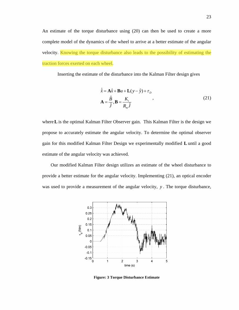
An estimate of the torque disturbance using (20) can then be used to create a more

complete model of the dynamics of the wheel to arrive at a better estimate of the angular

velocity. Knowing the torque disturbance also leads to the possibility of estimating the

traction forces exerted on each wheel.

Inserting the estimate of the disturbance into the Kalman Filter design gives

ˆ ˆ ˆ( )

ˆ,ˆ ˆ

D

t

m

x x u y y

KBJ R J

τ= + + − +

= =

A B L

A B, (21)

where L is the optimal Kalman Filter Observer gain. This Kalman Filter is the design we

propose to accurately estimate the angular velocity. To determine the optimal observer

gain for this modified Kalman Filter Design we experimentally modified L until a good

estimate of the angular velocity was achieved.

Our modified Kalman Filter design utilizes an estimate of the wheel disturbance to

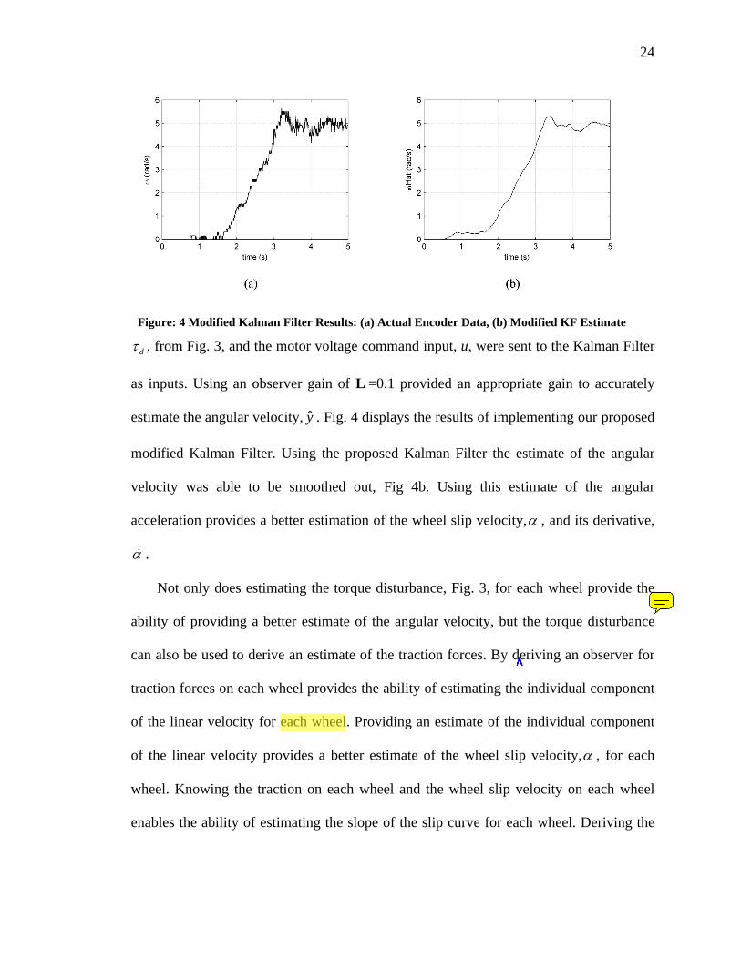
provide a better estimate for the angular velocity. Implementing (21), an optical encoder

was used to provide a measurement of the angular velocity, y . The torque disturbance,

Figure: 3 Torque Disturbance Estimate

24

dτ , from Fig. 3, and the motor voltage command input, u, were sent to the Kalman Filter

as inputs. Using an observer gain of L =0.1 provided an appropriate gain to accurately

estimate the angular velocity, y . Fig. 4 displays the results of implementing our proposed

modified Kalman Filter. Using the proposed Kalman Filter the estimate of the angular

velocity was able to be smoothed out, Fig 4b. Using this estimate of the angular

acceleration provides a better estimation of the wheel slip velocity,α , and its derivative,

α .

Not only does estimating the torque disturbance, Fig. 3, for each wheel provide the

ability of providing a better estimate of the angular velocity, but the torque disturbance

can also be used to derive an estimate of the traction forces. By deriving an observer for

traction forces on each wheel provides the ability of estimating the individual component

of the linear velocity for each wheel. Providing an estimate of the individual component

of the linear velocity provides a better estimate of the wheel slip velocity,α , for each

wheel. Knowing the traction on each wheel and the wheel slip velocity on each wheel

enables the ability of estimating the slope of the slip curve for each wheel. Deriving the

Figure: 4 Modified Kalman Filter Results: (a) Actual Encoder Data, (b) Modified KF Estimate

25

observer to estimate the traction forces from the estimate of the torque disturbance is a

subject for future research.

26

2.5. Output Feedback Control

To assure our traction estimation algorithm provides the ability of measuring traction

loss the full spectrum of the slip curve must be explored. Wheel slip, therefore, has to

range from zero to one which implies that α has to range from zero to α ω= . To

accurately control the angular velocity of the wheel we propose a control law which

tracks a desired reference velocity. Our control law uses linearization to drive the angular

velocity to the desired reference.

Letting the ideal motor model described in (18) take the form

ˆˆ ˆ

t

m

KB uJ R J

θ θ= − + , (22)

whereθ is the angle of the wheel, we desire to track a reference trajectory, rθ . For the

wheel to follow the desired angular trajectory the voltage required to produce that angle

can be determined from

ˆˆ ˆ

tr r

m

KB uJ R J

θ = , (23)

where ru is the required voltage input. Letting

1

2

,

,r

r

r

x

xv u u

θ θ

ω θ

= −

= −= −

(24)

transforms the ideal motor model to

27

1 2

2 2

1

ˆ( )ˆ ˆ

tr

m

x x

KBx x vJ R J

y x

θ

=

= − + +

=

(25)

To stabilize the transformed system let

1v Ky Kx= − = − . (26)

Substituting the control law into the transformed state model and performing linearization

of the model about the origin yields

( ) ,00 1

ˆ ,0 ˆˆ

t

m

x K x

KBR JJ

= −

⎡ ⎤⎡ ⎤⎢ ⎥⎢ ⎥= = ⎢ ⎥⎢ ⎥− ⎢ ⎥⎢ ⎥⎣ ⎦ ⎣ ⎦

A B

A B, (27)

where K is designed to make (27) stable.

The overall control law then becomes

1ru u Kx= − . (28)

Using this control law provides the ability of tracking an angular reference. The

benefit of this controller is it provides the desired voltage command to drive the system to

the desired angular velocity. If there is tracking error due to an unknown disturbance the

control gain K modifies the control input to push harder or relaxes the command

depending on the sign of the error.

28

The results in Fig. 4 were used with this control law. The remaining figures in the

angular velocity results were also used with this control law. The values for the gain K

were determined through experimentation. With K=2 the controller was able to

effectively drive the system to a desired steady state value of 5rad/s.

29

2.6. Experimental Results

2.6.1. Methods and Procedures

To validate our traction estimation, algorithm tests were performed on a single axel

mobile robot. Fig. 5 provides visual description of the experimental setup. A trailing

wheel was mounted on the back of the robot for stabilization. The control of the robot

was achieved using a tether via dSpace™ 1103 DSP, and power was provided externally.

Two geared DC motors were used to drive the robot. Sensing of wheel odometry was

accomplished using encoders, and sensing of the dynamics of the robot was

accomplished with a single axis accelerometer. Power was provide to the accelerometer

by a 7.2v RC car battery coupled to a 5v regulator. The robot was coupled to a linear

Figure: 5 Experimental Setup

30

potentiometer that measured displacement and exerted and increasing spring force as the

potentiometer was extended. Thus, a known external force was applied. The gain for

linear displacement was found to be 35mm/V, while the force profile was parabolic, Fig

6. Using least squares regression the coefficients for the curve was estimated to calculate

force profile of the linear potentiometer.

With the retarding force acting on the robot, the linear travel of the robot was

dependant on surface conditions. The surface conditions were picked to maintain that the

maximum traction force was less than the maximum tether force. Allowing this

relationship to hold provided an experiment which forced pure slip on the wheels of the

mobile robot. The sampling rate for the experiments was conducted at 100 Hz to limit

sensor noise from the encoder/ accelerometer and to reduce chatter from the controller.

With this frequency, however, the sensor noise still needed to be filtered to provide an

accurate measurement of traction loss. To reduce sensor noise from the encoders, our

proposed modified Kalman Filter was designed to smooth out the angular velocity data.

The accelerometer data was also filtered with a cutoff frequency of 50rad/s. The output of

Figure: 6 Linear Potentiometer Force Profile

31

the Kalman Filter was fused with the filtered data from the accelerometer to calculate the

value of traction loss.

To ensure repeatable wheel slip, our proposed output linear feedback integral

controller was designed drive the angular velocity of the wheel to a desired trajectory.

This controller provided repeatable wheel slip in the presence of the variable tether force

given the prescribed trajectory. This controller provided zero steady state error for a

desired trajectory. A piece wise trajectory was designed, which started with the initial

conditions of the robot being zero and ended with a steady state angular velocity. The

controller was first tested without the tether with the control gain K=2. With a working

controller, the robot was connected to the tether and tests were performed on carpet and

sand with a depth of 1cm using the same control gains. Results for the tests were

compiled offline.

32

2.6.2. Results and Discussion

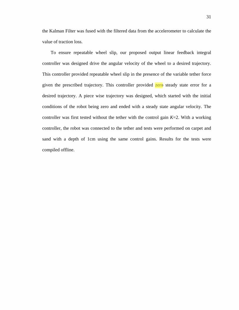
Implementing our traction estimation technique, we can determine a neighborhood,

N, where traction loss is occurring. Fig. 7 displays a table of figures representing

comparable results for tests conducted on carpet. Each figure in the table contains two

vertical lines which are placed at specific instances in time. These vertical lined define

the limits of a neighborhood N where 21 2{ , ( ) | }N t f t R t t t= ∈ ≤ ≤ . The left figure

displays the angular velocity and the relative ground velocity compared to the desired

angular velocity reference. The center figure displays the results for wheel slip

velocity,α , and the right figure displays the result for the derivative of the wheel slip

velocity α . The neighborhood, N, can be defined on both carpet and sand to estimate

when traction loss is occurring. Justification of our algorithm will be contained to the

results on carpet since these results typify the performance of our traction estimation

algorithm, Fig. 7. After proving the validity of our traction estimation algorithm on carpet

the results from our experiments on sand will be discussed.

Figure: 7 Traction Estimation Algorithm Results on Carpet: (left) Angular Velocity and Ground Velocity Measurement vs. Desired Trajectory, (center) wheel slip velocityα , (right) wheel slip

acceleration α

33

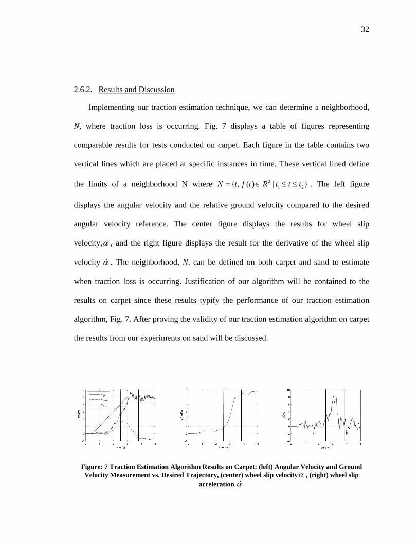
Figure 7 displays comparable results on carpet. As can be seen from Fig. 7, the two

vertical lines define a neighborhood N where { }2, ( ) | 2.3 3.9N t f t R t= ∈ ≤ ≤ . Before

2.3s there is no depreciable change between the angular velocity of the wheel, wheelω , and

the relative ground velocity, accω . As the response of the wheel starts to track the desired

reference velocity, there is a positive increase in the angular velocity at ~1.5s. The

relative ground velocity too has a positive increase at this instance in time.

From examining Pacejka’s slip curve, wheel slip has to occur to maximize traction

force. Before t=2.3s, the magnitude of the wheel slip velocity,α , is small and derivative

of the wheel slip velocity, α , is near zero. The wheel slip velocity, α , being small,

determines the amount of slip to initially pull the tether. The measurement of α being

near zero demonstrates that though wheel slip is occurring it is not changing quickly. The

traction force, therefore, is sufficient to overcome the tether. This same argument can be

made upon inspection of the angular velocity and the relative ground velocity. Since the

angular velocity and the relative ground velocity are monotonically increasing, there is no

traction loss. Fig. 8 shows that before 2.3s the mobile robot has displaced from its initial

Figure: 8 Linear Potentiometer Data for Carpet: (right) Position Data, (left) Force Data

34

position, 0mm, to a displacement of ~55mm. The force profile before 2.3s has increased

from zero ~11N.

In the region N, however, traction loss is occurring. As the tracking controller drives

the motors to the desired reference, the relative ground velocity, however, does not

coincide with the response of the angular velocity, Fig. 7. The response of the relative

ground velocity reaches a maximum at approximately 2.8s and quickly drops to zero. The

reduction in linear velocity, therefore, is due to wheel slip resulting from traction loss.

The value ofα in this neighborhood has dramatically increased. Since there is a change

in α , this change is represented inα . In this neighborhood, α forms a positive parabolic

curve. This is expected because there is a positive change in angular velocity while there

is a decrease in relative ground velocity. This significant change in α demonstrates that

traction loss is occurring in the neighborhood N. In this neighborhood, the traction

available on the surface is not sufficient to dominate over the rise in the tether force,

Fig.6, since the displacement, x, and the force, F, have reached steady state at t=3.9s.

Traction loss, therefore, is occurring in the neighborhood N.

At 3.9 seconds, the traction force and the tether force have reached equilibrium. The

equilibrium between the tether and traction force, therefore, results in driving the relative

ground velocity to zero. The angular velocity too has been driven to the steady state

reference velocity. The system, therefore, is in pure slip. Since the angular velocity and

the relative ground velocity are at steady state, the derivative of the wheel slip

velocity,α , is approximately zero. An important note is that the value of α at 3.9t > is

equivalent to the value of α at 0 2.3t< < . Traction loss, therefore, after t>3.9s cannot be

determined by α alone. The only metric which can be used to verify traction loss has

35

occurred is by inspection of α . At steady state, α ω= . With wheel slip velocity,α ,

equating to the angular velocity defines that the system is in pure slip and traction loss

has transpired.

Upon inspection of Fig. 7 and Fig. 8, it can be seen that traction loss can be

contained to a neighborhood N. The neighborhood, however, does not provide

quantitative data representing traction loss like the derivative of the slip curve, though it

does provide a qualitative representation of traction loss. Traction loss does not occur at

t=2.3s but traction loss is occurring by 3.9s. Within this neighborhood the relative

velocity of the curve has reached a maximum and is also driven to zero, Fig 7. The

displacement and the force also reach steady state by 3.9s. The neighborhood, therefore,

only provided qualitative data representing when traction loss is occurring.

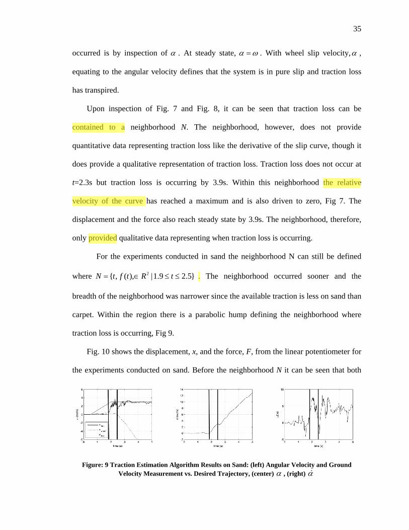
For the experiments conducted in sand the neighborhood N can still be defined

where 2{ , ( ), |1.9 2.5}N t f t R t= ∈ ≤ ≤ . The neighborhood occurred sooner and the

breadth of the neighborhood was narrower since the available traction is less on sand than

carpet. Within the region there is a parabolic hump defining the neighborhood where

traction loss is occurring, Fig 9.

Fig. 10 shows the displacement, x, and the force, F, from the linear potentiometer for

the experiments conducted on sand. Before the neighborhood N it can be seen that both

Figure: 9 Traction Estimation Algorithm Results on Sand: (left) Angular Velocity and Ground Velocity Measurement vs. Desired Trajectory, (center) α , (right) α

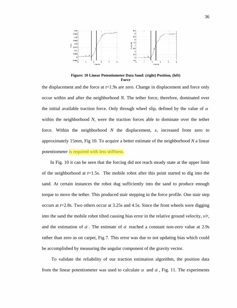
36

the displacement and the force at t<1.9s are zero. Change in displacement and force only

occur within and after the neighborhood N. The tether force, therefore, dominated over

the initial available traction force. Only through wheel slip, defined by the value of α

within the neighborhood N, were the traction forces able to dominate over the tether

force. Within the neighborhood N the displacement, x, increased from zero to

approximately 15mm, Fig 10. To acquire a better estimate of the neighborhood N a linear

potentiometer is required with less stiffness.

In Fig. 10 it can be seen that the forcing did not reach steady state at the upper limit

of the neighborhood at t=1.5s. The mobile robot after this point started to dig into the

sand. At certain instances the robot dug sufficiently into the sand to produce enough

torque to move the tether. This produced stair stepping in the force profile. One stair step

occurs at t=2.8s. Two others occur at 3.25s and 4.5s. Since the front wheels were digging

into the sand the mobile robot tilted causing bias error in the relative ground velocity, v/r,

and the estimation of α . The estimate of α reached a constant non-zero value at 2.9s

rather than zero as on carpet, Fig 7. This error was due to not updating bias which could

be accomplished by measuring the angular component of the gravity vector.

To validate the reliability of our traction estimation algorithm, the position data

from the linear potentiometer was used to calculate α and α , Fig. 11. The experiments

Figure: 10 Linear Potentiometer Data Sand: (right) Position, (left) Force

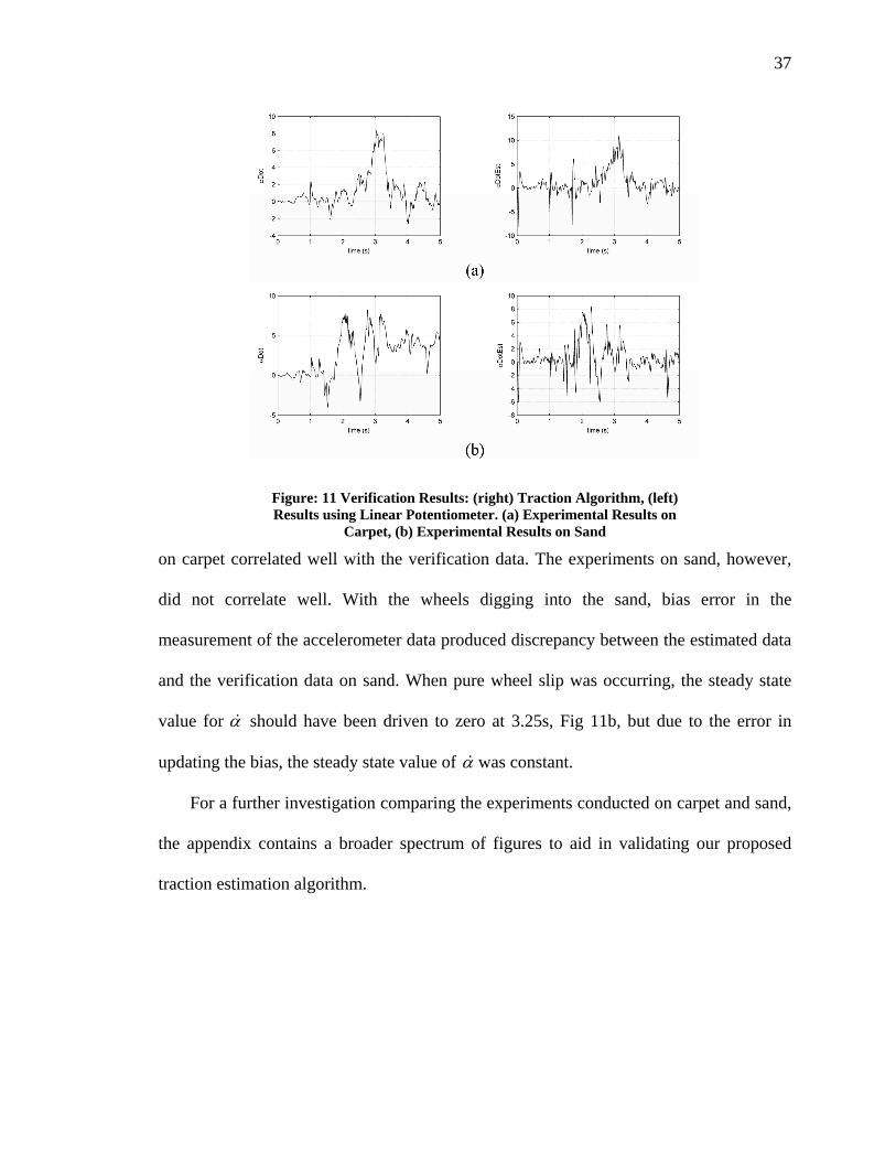
37

on carpet correlated well with the verification data. The experiments on sand, however,

did not correlate well. With the wheels digging into the sand, bias error in the

measurement of the accelerometer data produced discrepancy between the estimated data

and the verification data on sand. When pure wheel slip was occurring, the steady state

value for α should have been driven to zero at 3.25s, Fig 11b, but due to the error in

updating the bias, the steady state value of α was constant.

For a further investigation comparing the experiments conducted on carpet and sand,

the appendix contains a broader spectrum of figures to aid in validating our proposed

traction estimation algorithm.

Figure: 11 Verification Results: (right) Traction Algorithm, (left) Results using Linear Potentiometer. (a) Experimental Results on

Carpet, (b) Experimental Results on Sand

38

3. TRACTION CONTROL OF A MOBILE ROBOT

3.1. Introduction

In designing a controller which compensated for traction loss, a method for sensing

traction loss must first be obtained. In Chapter 1 it was shown that by determining the

sign of slope of the Pacejka’s Tire Model traction loss was able to be estimated. If the

slope of the slip curve was positive, traction loss was not occurring. But, if the slope of

the slip curve was negative, traction loss was occurring. The slope of the slip curve,

however, becomes unbounded when the derivative of the wheel slip is constant.

Attempting to drive wheel slip to some constant value using a proposed control law

founded on wheel slip negates the ability of estimating traction loss since the slope of the

slip curve is unbounded.

We have proposed a traction estimation algorithm that is able to accurately

determine when traction loss is occurring. Our traction estimation algorithm couples the

vehicle dynamics using Pacejka’s Tire model. The effects of traction loss, therefore, are

built into our traction estimation algorithm since estimating the variables of our algorithm

can be obtained using onboard sensors. Our traction estimation algorithm was shown to

define a neighborhood to qualitatively show when traction loss is occurring.

39

Using our traction estimation algorithm we propose a continuous robust controller

which converges α to a neighborhood. By containing α to a desired neighborhood also

implies there is an upper bound on the size of α . Having an upper bound on α enables

our control law to maximize traction since estimating the value α contains the effects of

Pacejka’s Tire Model.

A unique aspect of our controller is it works jointly with a tracking controller. The

tracking controller’s purpose is to drive the angular velocity of the wheel to a desired

reference. When traction loss is occurring our proposed control law is able maintain

traction without fighting with the tracking controller.

In this chapter we present two controllers. We will first present our tracking

controller. Using this controller and our proposed traction estimation algorithm we will

propose a continuous traction controller which converges α to a neighborhood. Our

experimental setup will be explained, and results from our proposed traction control law

will be given.

A representation of our proposed control law is provided in Fig 12. The output of the

plant model provides measurement of the angular velocity,ω , from an optical encoder,

and a measurement of the acceleration, a, using an accelerometer. The angular velocity

signal is sent to our proposed robust tracking controller to determine the control input, ψ ,

required to follow the predetermined trajectory. The angular velocity signal is also fed

indo our modified Kalman Filter which is comprised of a torque disturbance observer and

a Kalman Filter. The torque disturbance observer outputs the disturbance torque, dτ ,

using the angular velocity and the plant input, τ . Using our modified Kalman Filter we

obtain a better estimate of our angular velocity data, ω . Both the estimate of the angular

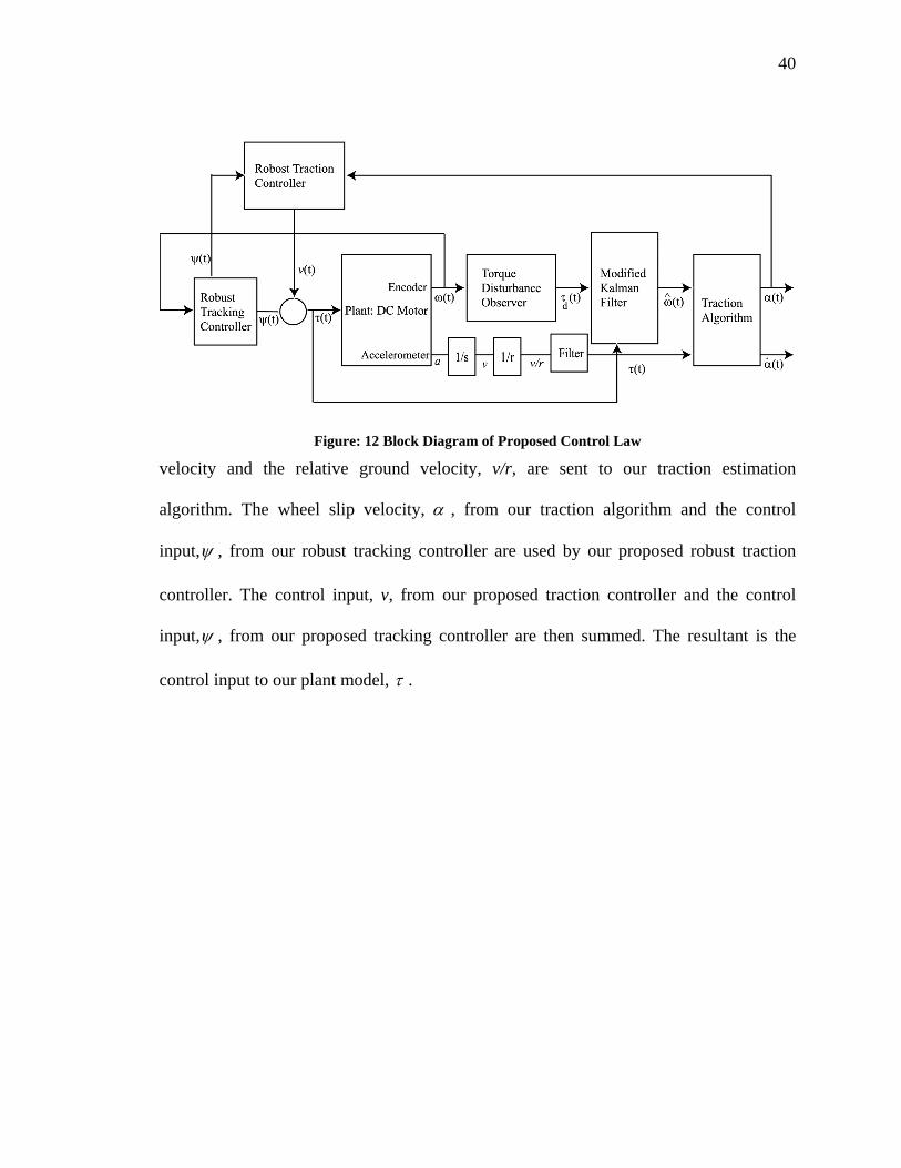
40

velocity and the relative ground velocity, v/r, are sent to our traction estimation

algorithm. The wheel slip velocity, α , from our traction algorithm and the control

input,ψ , from our robust tracking controller are used by our proposed robust traction

controller. The control input, v, from our proposed traction controller and the control

input,ψ , from our proposed tracking controller are then summed. The resultant is the

control input to our plant model, τ .

Figure: 12 Block Diagram of Proposed Control Law

41

3.2. Traction Control Design

3.2.1. Robust Tracking Control Design

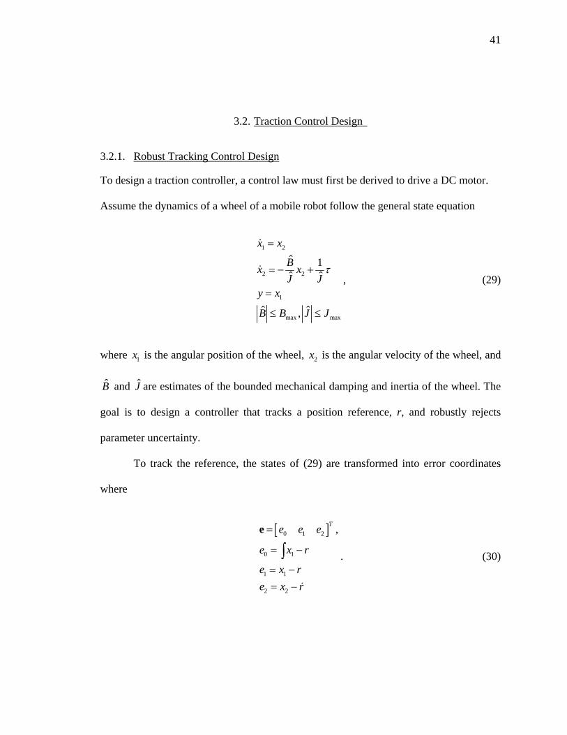
To design a traction controller, a control law must first be derived to drive a DC motor.

Assume the dynamics of a wheel of a mobile robot follow the general state equation

1 2

2 2

1

max max

ˆ 1ˆ ˆ

ˆ ˆ,

x x

Bx xJ J

y x

B B J J

τ

=

= − +

=

≤ ≤

, (29)

where 1x is the angular position of the wheel, 2x is the angular velocity of the wheel, and

B and J are estimates of the bounded mechanical damping and inertia of the wheel. The

goal is to design a controller that tracks a position reference, r, and robustly rejects

parameter uncertainty.

To track the reference, the states of (29) are transformed into error coordinates

where

[ ]0 1 2

0 1

1 1

2 2

,Te e e

e x r

e x re x r

=

= −

= −= −

∫e

. (30)

42

Taking the derivative of (30) yields

0 1

1 2

3 1 2 2

1 2

( )ˆ 1,ˆ ˆ

e ee ee x r

BJ J

θ θ τ

θ θ

=== + −

= − =

(31)

Let τ take the following form

vτ φ= + , (32)

where φ is a feedback linearization controller whose purpose is to stabilize the origin of

(30) and v is a robust controller that compensates for parameter uncertainty. The control

input then becomes,

1 12

1 3( ) tanh( )sx Ks rτ θ βθ ε

= − + − − , (33)

where s is the sliding manifold,

0 0 1 1 2s Ke K e K e e= = + + , (34)

and K is designed to make (31) stable and guarantees the an error convergence on the

surface when s=0 shown in (33).

43

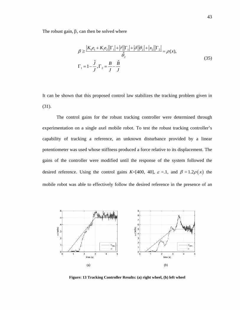
The robust gain, β, can then be solved where

0 1 1 2 1 1 2 2 2

2

1 2

( ),ˆ

ˆ ˆ1 ,

K e K e r xx

J B BJ J J

δ θβ ρ

θ+ Γ + Γ + + Γ

≥ =

Γ = − Γ = −

(35)

It can be shown that this proposed control law stabilizes the tracking problem given in

(31).

The control gains for the robust tracking controller were determined through

experimentation on a single axel mobile robot. To test the robust tracking controller’s

capability of tracking a reference, an unknown disturbance provided by a linear

potentiometer was used whose stiffness produced a force relative to its displacement. The

gains of the controller were modified until the response of the system followed the

desired reference. Using the control gains K=[400, 40], ε =.1, and β = ( )1.2 xρ the

mobile robot was able to effectively follow the desired reference in the presence of an

Figure: 13 Tracking Controller Results: (a) right wheel, (b) left wheel

44

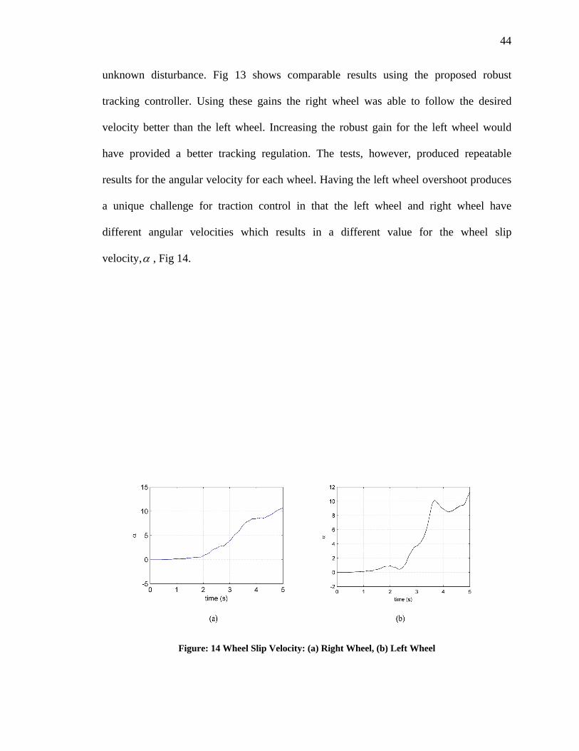
unknown disturbance. Fig 13 shows comparable results using the proposed robust

tracking controller. Using these gains the right wheel was able to follow the desired

velocity better than the left wheel. Increasing the robust gain for the left wheel would

have provided a better tracking regulation. The tests, however, produced repeatable

results for the angular velocity for each wheel. Having the left wheel overshoot produces

a unique challenge for traction control in that the left wheel and right wheel have

different angular velocities which results in a different value for the wheel slip

velocity,α , Fig 14.

Figure: 14 Wheel Slip Velocity: (a) Right Wheel, (b) Left Wheel

45

3.2.2. Traction Control Design

To provide a mobile robot the ability of maximizing traction, there must be a degree

of wheel slip. In this section we propose a continuous Lyapunov Redesign controller

which will confine α to a neighborhood. The size of the neighborhood is dependant on

the control gain of the continuous controller.

Our proposed traction estimation algorithm introduced a modified, first order,

differential equation,

ˆ 1 ( )ˆ ˆb Fm m

α α τ= − + − (36)

where

ˆˆBJ

ω ω τ+ = , (37)

and

46

,v vr r

α ω α ω= − = − (38)

To derive a control law based upon (36) a function has to be defined which

models the forcing applied to the system model. Using the causal relationship from

Pacejka’s Tire Model a proposed function can be derived.

The boundary conditions of the function has to allow perfect mapping between

the torque acting on the wheel and the forcing applied by the wheel when wheel slip is

zero. When slip is unity implies the linear velocity is zero and no torque from the motor

is mapped to the forcing applied by the wheel.

Our traction estimation algorithm does not provide such simple boundary

conditions since α is not bounded between zero and one. To provide a function whose

mapping of wheel torque varies between the limits of perfect mapping to no mapping,

assume the forcing applied to the system model in (36) follows the general form,

( ) ,0 ( ) 1F g gJτα α= ≤ ≤ , (39)

where ( )g α is a smooth, bounded, class KL function. The purpose in defining the forcing

in (39) is to allow a perfect mapping of wheel torque when ( )g α is unity and no

mapping of wheel torque when ( )g a is zero. For simplicity it is assumed

( )( ) ag e αα −= . (40)

The form of (40) takes this form due to the ability of modifying the constant, a, to define

the value of α that settles near zero, sα , where 4 /s aα = . Applying (39) to (36) modifies

the traction estimation function to

47

ˆ 1 (1 ( ))ˆb gm J

α α α τ= − + − , (41)

where τ is the robust tracking controller defined previously. To compensate for traction

loss, let

vτ ψ= + , (42)

where ψ is the control input to stabilize the tracking problem of (37), and v is the control

input to stabilize (41). Substituting this control law into (41) gives,

ˆ 1 [1 ( )]( )ˆb g vm J

α α α ψ= + − − . (43)

Given this general equation for traction estimation, the robust tracking control input

ψ can be viewed as a known, bounded disturbance to the system. The control design

problem then becomes one of providing a control law v to stabilize the system under this

disturbance. To achieve this, the control law needs to dominate the disturbance.

To derive a control law which will dominate over the disturbance generated from

the robust tracking controller, consider the Lyapunov candidate function,

212

V α= . (44)

Taking the derivative of (44) gives

2ˆ

[1 ( )]( )ˆˆbV g vm J

ααα α α ψ= = − + − + . (45)

48

To stabilize the system in (43), the derivative of the Lyapunov candidate function must

be negative definite.

To accomplish this, let

,wvw

η= − (46)

where

0

0

,1

,

[1 ( )]ˆ

kv k v

w gJ

ρη

τ δ ρα α

≥−

+ ≤ +

= −

. (47)

Substituting the control law into (45) produces

22

2

2

ˆ,

ˆˆ

,ˆˆ

.ˆ

b wV wm w

b w wmbm

α η τ

α η η

α

≤ − − +

≤ − − +

≤ −

(48)

which shows the derivative of the Lyapunov function is negative definite in the

neighborhood { }N Rα= ∈ . This control law guarantees the stabilization of the system

under the bounded disturbance τ .

This controller, however, drives alpha to the origin. We desire to drive alpha to a

neighborhood. To accomplish this, we provide a continuous controller,

3tanh( )wv ηε

= − , (49)

49

where ε is some tuned parameter. The gain of three is in the numerator to allow the

hyperbolic tangent to approximately equal one when w ε= .

Since the control law is continuous, the system will converge to a bounded

neighborhood. To estimate the range of this neighborhood, the continuous control law

must be substituted into the Lyapunov candidate function. Performing this operation

modifies the Lyapunov function to

2 200

ˆ ˆ(1 ) , 0ˆ ˆ4 4

kb bV km m

ε εα α− −≤ − + ≤ + = . (50)

The surface where 0V = defines an estimate of the contour defining the boundary of the

neighborhood. The boundary of the neighborhood which defined the convergence of the

continuous controller is

2ˆ

ˆ 4bm

εα ≤ . (51)

The estimate of the neighborhood in (51), however, is a conservative estimate. Being

a conservative estimate the actual neighborhood will be larger. Only through

implementing our continuous traction controller through experimentation can the actual

size of the neighborhood be defined. (51), however, does explain a certain aspect of the

size of the neighborhood. As the value of ε increases the size of the neighborhood also

increases. The results from experimentation, therefore, should show that as ε increases

the size of the neighborhood should also increase.

50

In the design of our control law, we have the ability to compensate for traction loss

and to dominate over the robust tracking controller. The traction controller has also been

designed to be continuous and ensure the system will converge within a defined

neighborhood. When traction loss is not prevalent, this control law will be small

compared to the robust tracking controller. The robust tracking controller will then

dominate the system and will track the desired reference.

51

3.3. Experimental Evaluation

3.3.1. Methods and Procedures

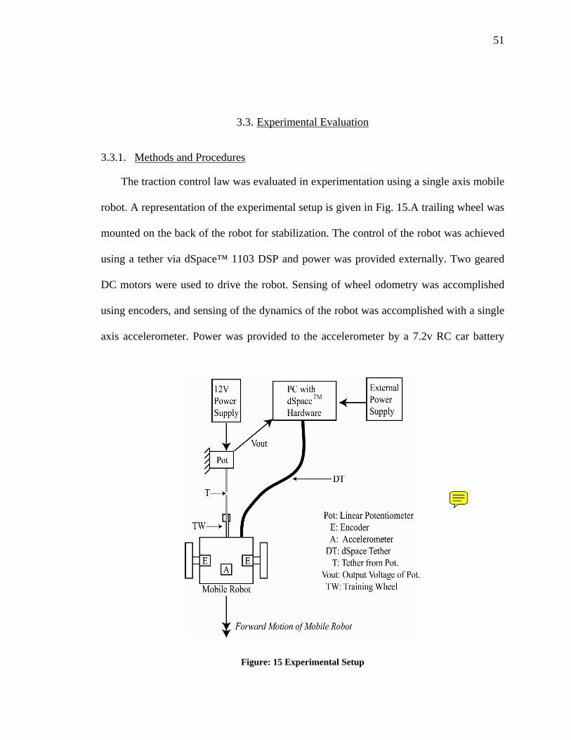
The traction control law was evaluated in experimentation using a single axis mobile

robot. A representation of the experimental setup is given in Fig. 15.A trailing wheel was

mounted on the back of the robot for stabilization. The control of the robot was achieved

using a tether via dSpace™ 1103 DSP and power was provided externally. Two geared

DC motors were used to drive the robot. Sensing of wheel odometry was accomplished

using encoders, and sensing of the dynamics of the robot was accomplished with a single

axis accelerometer. Power was provided to the accelerometer by a 7.2v RC car battery

Figure: 15 Experimental Setup

52

coupled to a 5v regulator. To ensure wheel slip, a linear potentiometer was tethered to the

back of the trailing wheel’s frame. Using this sensor provided an accurate measurement

of displacement, and also provided the necessary disturbance of force to ensure wheel

slip. The sampling rate for the experiments was conducted at 100 Hz to limit sensor noise

from the encoder/ accelerometer and to reduce chatter from the controller. With this

frequency, however, the sensor noise still needed to be filtered to provide an accurate

measurement of traction loss. To reduce sensor noise from the encoders, a Kalman Filter

was designed to smooth out the angular velocity data. The accelerometer data was also

filtered with a second order filter with a cutoff frequency of 50rad/s. The output of the

Kalman Filter was fused with the filtered data from the accelerometer to calculate the

value of traction loss.

The tracking control law and the traction control law were evaluated using the

algorithm provided in Sect. (3.2.1) and Sect. (3.2.2). Tests were conducted on carpet,

which offered a surface with ample traction force. First, experiments were conducted on

carpet without the tether and without the traction control law. The purpose of this was to

determine the control gains for the tracking controller. Once the tracking controller

provided acceptable results on carpet without the tether, tests were conducted with the

tether. The control gains for the tracking controller were then modified to robustly reject

the disturbance from the tether.

The traction control law was then implemented on the robot with the tether. The

purpose of the experiments was to determine the balance necessary to effectively

dominate over the tracking controller when traction loss occurs. To accomplish this

certain parameters were modified. These parameters included varying the time constant,

53

a, from (40), the size of the continuous envelope, ε , from (49), and the dominance of the

robust gain, η , from (49). To evaluate the performance of the proposed tracking/traction

controller, several tests were conducted. The performance of the controller was

dependent on its ability to converge within the desired neighborhood by evaluating α

and evaluating the maximum force, F, and maximum displacement, x∆ . With each

control gain, several tests were conducted to acquire sufficient statistical data to

determine how the system reacted under these gains.

54

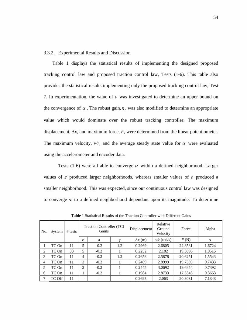
3.3.2. Experimental Results and Discussion

Table 1 displays the statistical results of implementing the designed proposed

tracking control law and proposed traction control law, Tests (1-6). This table also

provides the statistical results implementing only the proposed tracking control law, Test

7. In experimentation, the value of ε was investigated to determine an upper bound on

the convergence of α . The robust gain,η , was also modified to determine an appropriate

value which would dominate over the robust tracking controller. The maximum

displacement, ∆x, and maximum force, F, were determined from the linear potentiometer.

The maximum velocity, v/r, and the average steady state value for α were evaluated

using the accelerometer and encoder data.

Tests (1-6) were all able to converge α within a defined neighborhood. Larger

values of ε produced larger neighborhoods, whereas smaller values of ε produced a

smaller neighborhood. This was expected, since our continuous control law was designed

to converge α to a defined neighborhood dependant upon its magnitude. To determine

Table 1 Statistical Results of the Traction Controller with Different Gains

Traction Controller (TC) Gains Displacement

Relative Ground Velocity

Force Alpha No. System # tests

ε a γ ∆x (m) v/r (rad/s) F (N) α 1 TC On 11 5 -0.2 1.2 0.2969 2.6805 22.3581 1.6724 2 TC On 33 5 -0.2 1 0.2252 2.182 19.3696 1.9515 3 TC On 11 4 -0.2 1.2 0.2658 2.5878 20.6251 1.5543 4 TC On 11 3 -0.2 1 0.2469 2.8999 19.7339 0.7433 5 TC On 11 2 -0.2 1 0.2445 3.0692 19.6854 0.7392 6 TC On 11 1 -0.2 1 0.1984 2.8733 17.5346 0.3653 7 TC Off 11 - - - 0.2695 2.063 20.8081 7.1343

55

which neighborhood maximized traction forces,

the maximum displacement and the maximum

force were determined from the linear

potentiometer data. The control gains

[ , ] [5,1.2]ε η = produced the largest

displacement and the largest force. The other

control gains, though minimizing wheel slip, did

not perform as adequate as Test 1 or Test 6. The

performance of these controllers can be

explained using an analysis of the slip curve.

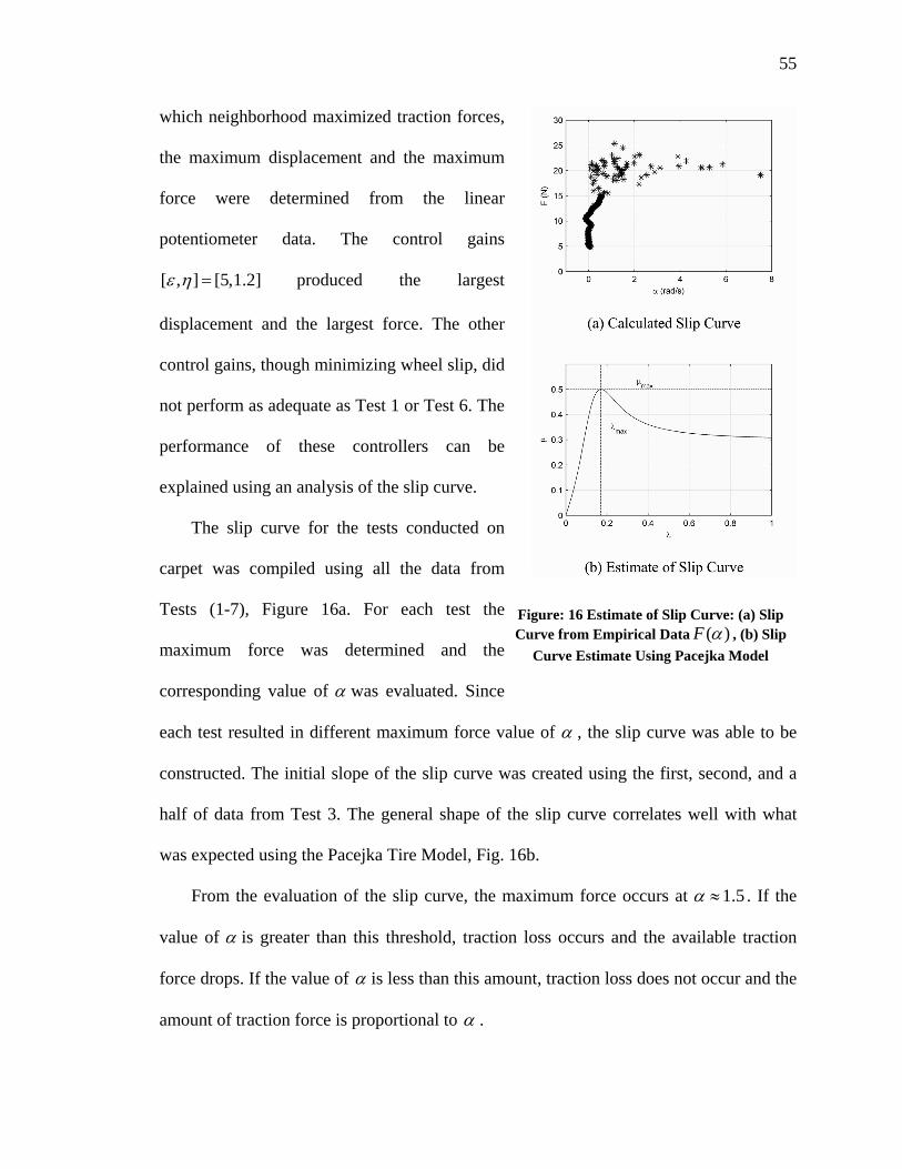
The slip curve for the tests conducted on

carpet was compiled using all the data from

Tests (1-7), Figure 16a. For each test the

maximum force was determined and the

corresponding value of α was evaluated. Since

each test resulted in different maximum force value of α , the slip curve was able to be

constructed. The initial slope of the slip curve was created using the first, second, and a

half of data from Test 3. The general shape of the slip curve correlates well with what

was expected using the Pacejka Tire Model, Fig. 16b.

From the evaluation of the slip curve, the maximum force occurs at 1.5α ≈ . If the

value of α is greater than this threshold, traction loss occurs and the available traction

force drops. If the value of α is less than this amount, traction loss does not occur and the

amount of traction force is proportional to α .

Figure: 16 Estimate of Slip Curve: (a) Slip Curve from Empirical Data ( )F α , (b) Slip

Curve Estimate Using Pacejka Model

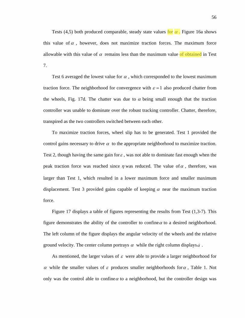
56

Tests (4,5) both produced comparable, steady state values for α . Figure 16a shows

this value of α , however, does not maximize traction forces. The maximum force

allowable with this value of α remains less than the maximum value of obtained in Test

7.

Test 6 averaged the lowest value for α , which corresponded to the lowest maximum

traction force. The neighborhood for convergence with 1ε = also produced chatter from

the wheels, Fig. 17d. The chatter was due to α being small enough that the traction

controller was unable to dominate over the robust tracking controller. Chatter, therefore,

transpired as the two controllers switched between each other.

To maximize traction forces, wheel slip has to be generated. Test 1 provided the

control gains necessary to drive α to the appropriate neighborhood to maximize traction.

Test 2, though having the same gain forε , was not able to dominate fast enough when the

peak traction force was reached since η was reduced. The value ofα , therefore, was

larger than Test 1, which resulted in a lower maximum force and smaller maximum

displacement. Test 3 provided gains capable of keeping α near the maximum traction

force.

Figure 17 displays a table of figures representing the results from Test (1,3-7). This

figure demonstrates the ability of the controller to confineα to a desired neighborhood.

The left column of the figure displays the angular velocity of the wheels and the relative

ground velocity. The center column portrays α while the right column displaysα .

As mentioned, the larger values of ε were able to provide a larger neighborhood for

α while the smaller values of ε produces smaller neighborhoods forα , Table 1. Not

only was the control able to confineα to a neighborhood, but the controller design was

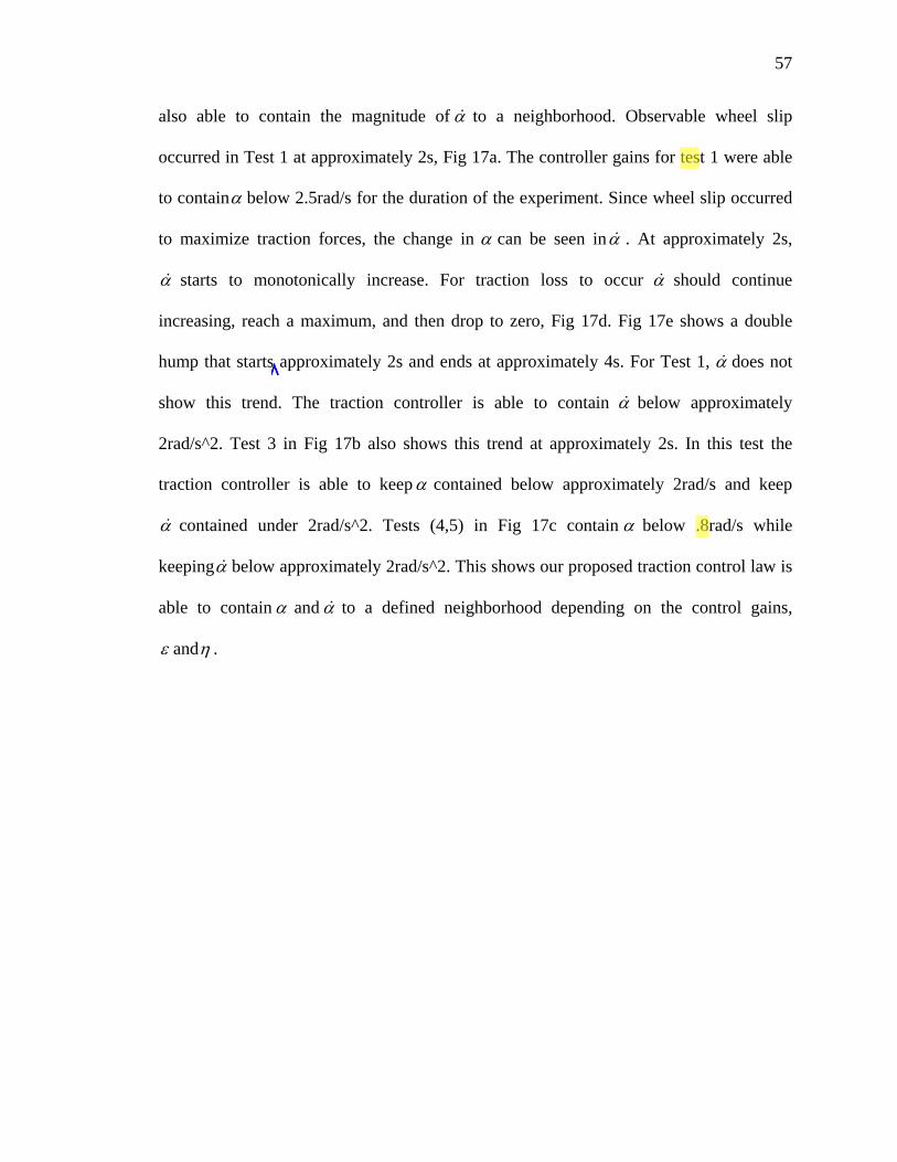
57

also able to contain the magnitude of α to a neighborhood. Observable wheel slip

occurred in Test 1 at approximately 2s, Fig 17a. The controller gains for test 1 were able

to containα below 2.5rad/s for the duration of the experiment. Since wheel slip occurred

to maximize traction forces, the change in α can be seen inα . At approximately 2s,

α starts to monotonically increase. For traction loss to occur α should continue

increasing, reach a maximum, and then drop to zero, Fig 17d. Fig 17e shows a double

hump that starts approximately 2s and ends at approximately 4s. For Test 1, α does not

show this trend. The traction controller is able to contain α below approximately

2rad/s^2. Test 3 in Fig 17b also shows this trend at approximately 2s. In this test the

traction controller is able to keep α contained below approximately 2rad/s and keep

α contained under 2rad/s^2. Tests (4,5) in Fig 17c contain α below .8rad/s while

keepingα below approximately 2rad/s^2. This shows our proposed traction control law is

able to contain α and α to a defined neighborhood depending on the control gains,

ε andη .

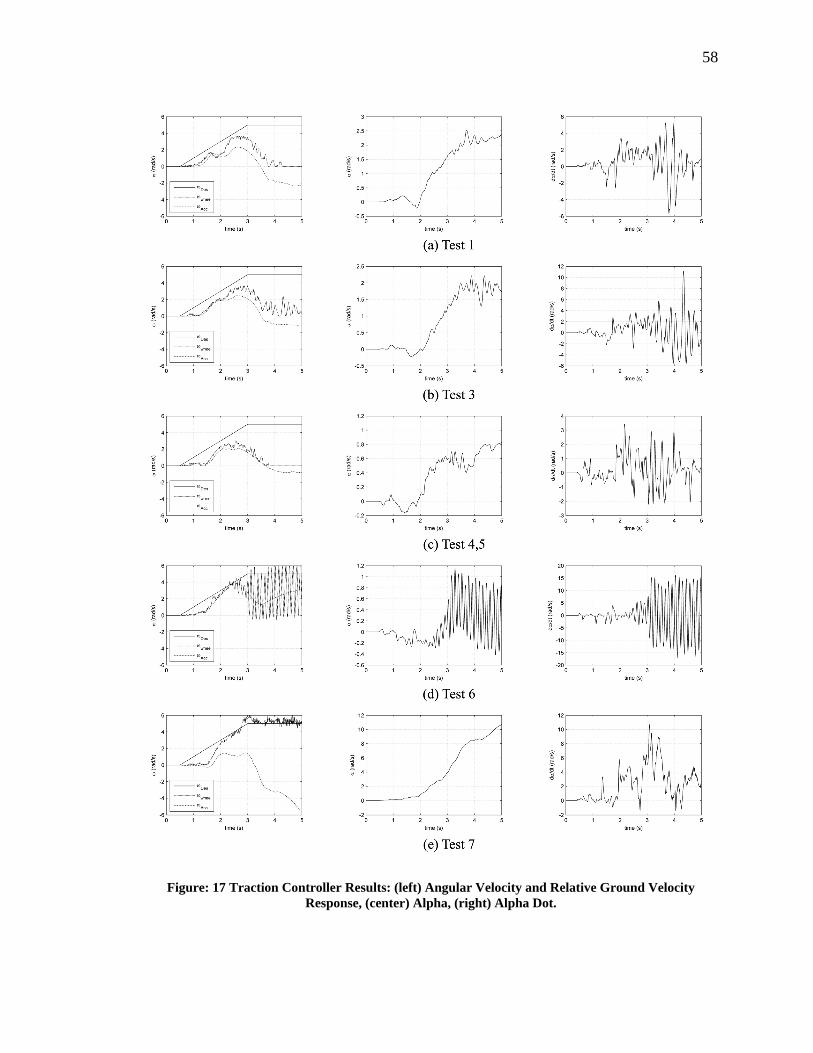
58

Figure: 17 Traction Controller Results: (left) Angular Velocity and Relative Ground Velocity Response, (center) Alpha, (right) Alpha Dot.

59

4. CONCLUSION AND FUTURE WORK

4.1. Traction Estimation

In achieving our goal of estimating the slope of Pacejka’s Tire Model we have

derived a new algorithm that replaces the estimation of the wheel slip ratio with the

wheel slip velocity. Our algorithm utilized the Pacejka’s Tire Model with vehicle

dynamics. The end result was a first order differential equation that coupled the

dynamics of the wheel with the dynamics of the vehicle. Our traction estimation

algorithm does not yet estimate the slope of the Pacejka’s Tire model to determine

traction loss, but it does provide a neighborhood where traction loss is occurring. Since

our traction estimation algorithm was observable using encoders for wheel odometry and

a single axis accelerometer for acceleration, the wheel slip velocity and its derivative

were able to be estimated.

To achieve an accurate estimate of traction loss using our proposed algorithm we

designed a modified Kalman Filter. The system model describing the dynamics of the

wheel is augmented by introducing an estimate of the unmodled torque disturbance.

Implementing this augmented system model resulted in providing a good estimate of the

angular velocity.

60

To validate our traction estimation algorithm, an output feedback controller was

designed to produce repeatable wheel slip by following a prescribed trajectory in the

presence of a tether. Providing experiments with repeatable wheel slip resulted in

repeatable results for estimating the wheel slip velocity and its derivative. Only by

providing a repeatable estimate of wheel slip and its derivative were we able to show that

traction loss was confined to a neighborhood whose bounds were two instances in time as

described in Fig 7 and 9.

Fusing the data from the modified Kalman Filter with the data from the single axis

accelerometer we showed that traction loss was detectable in a neighborhood.

Experiments conducted on carpet provided a surface that resulted good estimates of our

traction estimation variables α and α . Through the good estimates of α and α a

neighborhood was clearly defined when traction loss was occurring. A neighborhood

defining when traction loss transpired was also observable with the tests conducted on

sand. Sand, however, provided a surface that stressed the limits of our traction estimation

algorithm.

Bias drift caused poor estimation of the relative ground velocity. The bias drift

occurred from the mobile robot digging into the sand. With the mobile robot digging into

the sand the robot tilted and modified the angular component of gravity changing the bias

of the accelerometer. To compensate for the angular component of gravity we plan on

replacing the single axis accelerometer with a three axis internal measurement unit

(IMU). Using the IMU our traction control algorithm can continually update the bias of

the accelerometer to provide a correct estimate of α andα . Digging of the robot into the

61

sand, however, did not only present the necessity of updating the bias, but also introduced

the ability of modeling terrain topography.

Digging of the mobile robot is not the only terrain characteristic that can cause the

bias of the accelerometer to change due to the angular component of gravity. Rarely in an

actual environment will the terrain be hard and perfectly plane. A particular path may

include a change in the topology of the environment. The topology of the environment

will result in the mobile robot to pitch and roll which will change the bias of the

accelerometer. Through implementation of using the IMU, the angular component of

gravity can map the topography of the environment.

The experiments on sand also introduced the necessity of using a different linear

potentiometer. Since the available traction was less on sand than carpet, the linear

potentiometer dominated over the available traction on the sand. This resulted in the

robot only moving ~35mm for the duration of the experiment. To provide a better test

setup on sand, or other terrains where traction is low, a linear potentiometer with a lower

force profile will be used. We are hopeful this will result in a similar displacement/force

curve as on carpet.

To further validate our traction estimation, experimentation on multiple surfaces

needs to be explored. Estimating acceleration through the (IMU) will allow multiple

surfaces to be explored like gravel and rocks. Having a variety of linear potentiometers

will allow surfaces whose available traction is low, like ice and snow, to be tested.

Through these experiments we plan on showing these surfaces also contain a

neighborhood where traction loss is occurring.

62

The torque disturbance observer also opens research to be conducted on estimating

the terrain characteristics. Providing the terrain characteristics will result in the ability of

measuring the slope of the slip curve since both the traction and wheel slip velocity will

be known for each wheel. Providing that ability to control the slope of the slip curve for

each wheel will provide the ability of maximizing traction for each wheel.

By knowing the traction forces acting on each wheel a controller also can be

designed which provides the ability of following a desired path in the presence of traction

loss. For example, assume one wheel can only provide a certain amount of traction force

to aid in the forward progression of the vehicle. The other wheels, using the slope of the

slip curve, have the ability of providing more traction. Commands can, therefore, be

given to the other wheels to drive the robot in a particular direction. Thus, the

independently driven wheels maximize traction and work cooperatively in following a

desired path.

4.2. Traction Control

We have proposed a robust traction controller to provide maximize traction forces by

containing wheel slip velocity to a neighborhood. Unlike previous designed controllers

that drive wheel slip ratio to a desired reference, our control law confines the wheel slip

velocity to a neighborhood. Confining the wheel slip velocity to a neighborhood gives

liberty to the controller to keep the wheel slip velocity bound to a desired value if traction

loss is occurring. We are able, therefore, to use the whole region of Pacejka’s slip curve

where traction is available and, when necessary, ride the peak of the slip curve.

63

To alleviate the potential of our tracking controller and our traction controller from

battling, our proposed traction controller was designed to dominate over the proposed

robust tracking controller when traction loss was observed. Our traction controller was

designed to be continuous to allow wheel slip to be contained in a neighborhood. We

showed that by decreasing the control gains this neighborhood converged closer to the

origin. Small control gains, though shrinking the neighborhood closer to the origin, did

not maximize traction and produced chatter if the control gains became too small.

Estimating Pacejka’s Tire model from experimental results we showed that the larger

control gains were able to maximize traction. Maximizing the traction force on carpet

allowed the mobile robot to displace farther than without the traction controller.

Though experiments were limited to carpet, further testing on different surfaces is

required to explore our proposed traction control law. Providing tests on a variety of

surfaces will allow us to tune the control gains for different surfaces. By finding the

control gains that maximize traction on these surfaces provides the ability of designing a

control law that is capable of tuning the control gains to maximize traction. By designing

this control law with a Nonlinear Damping controller we will be able to reject unmodled

disturbances more effectively It will also smooth out the control input to the DC motors.

After designing this Nonlinear Damping controller we can experiment on surfaces

with different terrain characteristics. By providing the mobile robot with a specific path

that navigates through different types of terrain we hope to show with our enhanced

control law that the mobile robot will be able to follow the desired path while

maximizing traction forces.

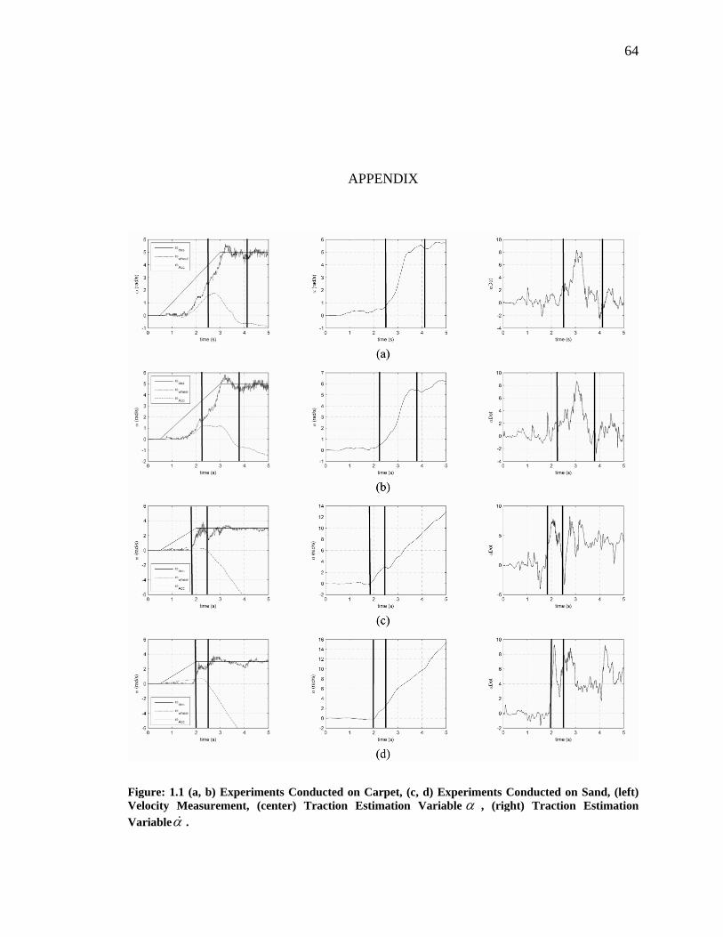
64

APPENDIX

Figure: 1.1 (a, b) Experiments Conducted on Carpet, (c, d) Experiments Conducted on Sand, (left) Velocity Measurement, (center) Traction Estimation Variable α , (right) Traction Estimation Variableα .

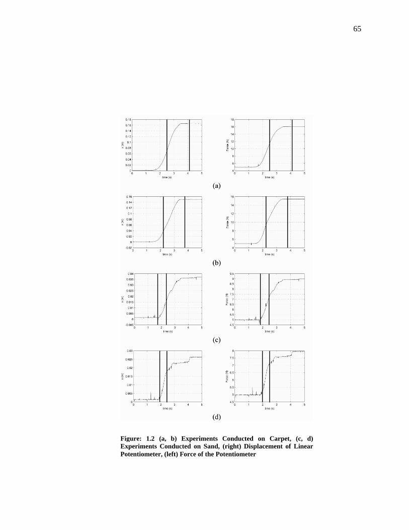
65

Figure: 1.2 (a, b) Experiments Conducted on Carpet, (c, d) Experiments Conducted on Sand, (right) Displacement of Linear Potentiometer, (left) Force of the Potentiometer

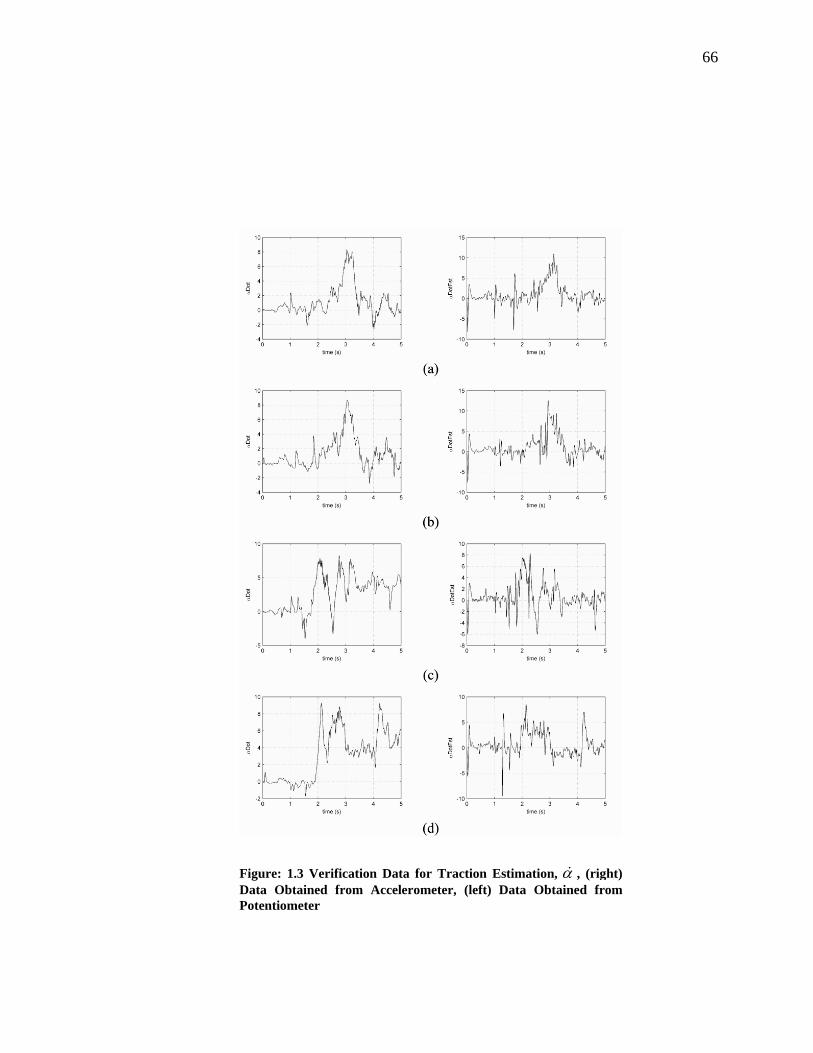
66

Figure: 1.3 Verification Data for Traction Estimation, α , (right) Data Obtained from Accelerometer, (left) Data Obtained from Potentiometer

67

REFERENCES

[1] R. Mukherjee, M. A. Minor, and J. T. Pukrushpan, "Simple motion planning

strategies for spherobot: a spherical mobile robot," presented at The 38th IEEE Conference on Decision and Control (CDC), Dec 7-Dec 10 1999, Phoenix, AZ, USA, 1999.

[2] X. Zhu, M. A. Minor, and S. Park, "Distributed robust control of compliant framed wheeled modular mobile robots," Journal of Dynamic Systems, Measurement and Control, Transactions of the ASME, vol. 128, pp. 489-498, 2006.

[3] E. R. Westervelt, J. W. Grizzle, and C. Canudas de Wit, "Switching and PI control of walking motions of planar biped walkers," IEEE Transactions on Automatic Control, vol. 48, pp. 308-312, 2003.

[4] Y. Zhou, "On the planar stability of rigid-link binary walking robots," Robotica, vol. 21, pp. 667-675, 2003.

[5] H. B. Pacejka and E. Bakker, "Magic formula tyre model," Vehicle System Dynamics

Proceedings of the 1st International Colloquium on Tyre Models for Vehicle Dynamics Analysis, Oct 21-22 1991, vol. 21, pp. 1-18, 1993.

[6] K. Iagnemma and S. Dubowsky, Mobile Robots in Rough Terrain: Estimation, Motion Planning, and Control with Application to Planetary Rovers: Springer, 2004.

[7] L. Ojeda, D. Cruz, G. Reina, and J. Borenstein, "Current-based slippage detection and odometry correction for mobile robots and planetary rovers," IEEE Transactions on Robotics, vol. 22, pp. 366-378, 2006.

[8] K. Iagnemma and S. Dubowsky, Mobile Robots in Rough Terrain: Estimation, Motion Planning and Control with Application to Planetary Rovers: Springer-Verlad Berlin Heidenlberg, 2004.

[9] J. H. a. M. Borm, C.H., "Determination of Optimal Measurment Configurations for Robot Calibration Based on Observability Measure," Intl. J. Robotics Research, vol. 10, pp. pg 51-63, 1991.

68

[10] M. R. Driels, and Pathre, "Significance of Observation Strategy on the Design of Robot Calibration Experiments," J. Robitic Systems, vol. 7, pp. pp 197-223, 1990.

[11] A. Nahvi, Hollerbach, J.M., and Hayward, V., "Closed-loop Kinematic Calibration of a Parallel-drive Shoulder Joint," presented at Proc. IEEE Intl. Conf. Robotics and Automation, San Deigo, May 8-13, 1994.

[12] D. H and B. BJ, "MEASUREMENT OF TIRE SHEAR FORCES," pp. 9, 1970.

[13] K. Chun and M. Sunwoo, "Wheel slip tracking using moving sliding surface," Proceedings of the Institution of Mechanical Engineers, Part D: Journal of Automobile Engineering, vol. 219, pp. 31-41, 2005.

[14] K. R. Buckholtz, "Reference Input Wheel Slip Tracking Using Sliding Mode Control," SAE Technical Paper Series, 2002-10-0301, 2002.

[15] C. Unsal and P. Kachroo, "Sliding mode measurement feedback control for antilock braking systems," IEEE Transactions on Control Systems Technology, vol. 7, pp. 271-281, 1999.

[16] N. Sarkar and X. Yun, "Traction control of wheeled vehicles using dynamic feedback approach," presented at Proceedings. 1998 IEEE/RSJ International Conference on Intelligent Robots and Systems. Innovations in Theory, Practice and Applications, 13-17 Oct. 1998, Victoria, BC, Canada, 1998.

[17] M. Tai and M. Tomizuka, "Robust longitudinal velocity tracking of vehicles using traction and brake control," presented at 6th International Workshop on Advanced Motion Control, Nagoya, Jpn, 2000.