Trade and Uncertainty∗

Dennis NovyUniversity of Warwick,

and CEPR †

Alan M. TaylorUniversity of California, Davis,

NBER, and CEPR ‡

September 2013Preliminary work in progress – comments welcome

AbstractWe offer a new explanation as to why international trade is so volatile in re-sponse to economic shocks. Our approach combines the uncertainty shockidea of Bloom (2009) with a model of international trade, extending the ideato the open economy. Firms import intermediate inputs from home or foreignsuppliers, but with higher costs in the latter case. Due to fixed costs of or-dering firms hold an inventory of intermediates. We show that in responseto an uncertainty shock firms optimally adjust their inventory policy by cut-ting their orders of foreign intermediates disproportionately strongly. In theaggregate, this response leads to a bigger contraction in international tradeflows than in domestic economic activity. We confront the model with newly-compiled monthly aggregate U.S. import data and industrial production datagoing back to 1962, and also with disaggregated data back to 1989. Our resultssuggest a tight link between uncertainty and the cyclical behavior of interna-tional trade.

Keywords: Uncertainty shock, trade collapse, inventory, real options, imports, intermedi-atesJEL Codes: E3, F1∗We thank the Souder Family Professorship at the University of Virginia, the Center for the Evolution of

the Global Economy at the University of California, Davis, and the Centre for Competitive Advantage inthe Global Economy (CAGE) at the University of Warwick for financial support. Travis Berge and Jorge F.Chavez provided valuable research assistance. For helpful conversations we thank Nicholas Bloom. We arealso grateful for comments by Nuno Limão, Giordano Mion, Veronica Rappoport, and John Van Reenen aswell as seminar participants at the 2011 Econometric Society Asian Meeting, the 2011 Econometric SocietyNorth American Summer Meeting, the 2011 LACEA-LAMES Meetings, the 2012 CAGE/CEP Workshop onTrade Policy in a Globalised World, the 2013 Economic Geography and International Trade (EGIT) ResearchMeeting, the NBER ITI Spring Meeting 2013, the 2013 CESifo Global Economy Conference 2013, the 2013Stanford Institute for Theoretical Economics (SITE) Summer Workshop on the Macroeconomics of Uncer-tainty and Volatility, the Monash-Warwick Workshop on Development Economics, Nottingham, Warwick,LSE and Oxford. All errors are ours.

†Email: d.novy@warwick.ac.uk‡Email: amtaylor@ucdavis.edu

1 Introduction

The recent global economic crisis was characterized by a sharp decline in economic out-put. However, the accompanying decline in international trade was even sharper, in somecases up to 50 percent. Standard models of international macroeconomics and interna-tional trade fail to account for the severity of the trade collapse.

In this paper, we attempt to explain why international trade is so volatile in responseto economic shocks. On the theoretical side, we combine the uncertainty shock conceptdue to Bloom (2009) with a model of international trade. Bloom’s (2009) real optionsapproach is motivated by high-profile events that trigger an increase in uncertainty aboutthe future path of the economy, for example the 9/11 terrorist attacks or the collapse ofLehman Brothers. In the wake of such events, firms adopt a ‘wait-and-see’ approach,slowing down their hiring and investment activities. Bloom (2009) shows that bouts oflarge uncertainty can be modeled as second moment shocks to demand or productivity andtypically lead to sharp recessions. Once the degree of uncertainty subsides, firms revertto their normal hiring and investment patterns, and the economy recovers.

We extend the uncertainty shock approach to the open economy. In contrast to Bloom’s(2009) closed-economy set-up, we develop a theoretical framework in which firms importintermediate inputs from foreign or domestic suppliers. This production structure is mo-tivated by the empirical observation that a large fraction of international trade consistsof capital-intensive intermediate goods such as car parts and electronic components orcapital investment goods.

Due to a fixed cost of ordering associated with transportation, firms hold an inventoryof intermediate inputs. Following the inventory model with time-varying uncertainty byHassler (1996), we show that in response to a large uncertainty shock to productivity orthe demand for final products, firms optimally adjust their inventory policy by cuttingtheir orders of foreign intermediates more strongly than orders for domestic intermedi-ates. In the aggregate, this differential response leads to a bigger contraction and subse-quently a stronger recovery in international trade flows than in domestic economic activ-ity. Thus, international trade exhibits more volatility than domestic economic activity. Ina nutshell, uncertainty shocks magnify the response of international trade.

Our model generates a set of additional predictions. First, the magnification effect isincreased by larger fixed costs of ordering. Intuitively, the larger the fixed costs of order-ing, the more reluctant firms are to order intermediate inputs from abroad if uncertaintyrises. This is a testable hypothesis to the extent that fixed ordering costs vary across do-mestic and foreign trading partners.

1

Second, the magnification effect is muted for industries characterized by high depreci-ation rates. Perishable goods are a case in point for extremely high depreciation rates. Thefact that such goods have to be ordered frequently means that importers have little choicebut to keep ordering them frequently even if uncertainty rises. Conversely, durable goodscan be considered as the opposite case of very low depreciation rates. Our model predictsthat for those goods we should expect the largest degree of magnification in response touncertainty shocks. Intuitively, the option value of waiting can be most easily realizedby delaying orders for durable goods. We find strong evidence of this pattern in the datawhen we examine the cross-industry response of imports to elevated uncertainty.

In sum, our model leads to various predictions in a unified framework. In contrastto conventional static trade models such as the gravity equation, we focus on the dy-namic response of international trade. In addition, we focus on second moment shocksand thus move beyond the first moment shocks traditionally employed in the literature.Our approach is relevant for researchers and policymakers alike who seek to understandthe recovery process in response to the Great Recession, and may also be relevant forunderstanding historical events like the Great Depression. It could also help predict thetrajectory of international trade in future economic crises.

On the empirical side, we confront the model with high-frequency monthly U.S. im-port and industrial production data going back to 1962. Our results suggest a tight linkbetween uncertainty shocks as identified by Bloom (2009) and the cyclical behavior ofinternational trade. That is, the behavior of trade can be well explained with standarduncertainty measures such as a VXO stock market volatility index. Bloom (2009) identi-fies 17 high-volatility episodes since the early 1960s such as the assassination of JFK, the1970s oil price shocks, the Black Monday of October 1987, the 1998 bailout of Long-TermCapital Management, 9/11 and the collapse of Lehman Brothers in September 2008. AsBloom (2009) shows, these high-volatility episodes are strongly correlated with alterna-tive indicators of uncertainty.

In particular, we argue that the Great Trade Collapse of 2008/09 can to a large extentbe explained by the large degree of uncertainty triggered by subprime lending and risingfurther up to, and especially after, the collapse of Lehman Brothers. According to ourempirical results, the unusually large trade collapse of 2008/09 is thus a response to theunusually large increase in uncertainty at the time.1 Although it stands out quantitatively,qualitatively the Great Trade Collapse is comparable to previous post-World War II slow-downs or contractions in international trade. In fact, our aim is to empirically account for

1Similarly, Bloom, Bond and Van Reenen (2007) provide empirical evidence that fluctuations in uncer-tainty can lead to quantitatively large adjustments of firms’ investment behavior.

2

trade recessions more generally, not only for the Great Trade Collapse. In addition, weconfirm the cross-industry predictions coming from our theoretical model.

We are certainly not the first authors to consider general uncertainty and real optionvalues in the context of international trade, but so far the literature has not examined therole of uncertainty shocks in an open-economy model of inventory investment. For exam-ple, Baldwin and Krugman (1989) adopt a real options approach to explain the hysteresisof trade in the face of large exchange rate swings but their model only features standardfirst moment shocks. More recently, the role of uncertainty has attracted new interest inthe context of trade policy and trade agreements (Handley 2012, Handley and Limão 2012and Limão and Maggi 2013). Similar to our approach, Taglioni and Zavacka (2012) empir-ically investigate the relationship between uncertainty and trade for a panel of countrieswith a focus on aggregate trade flows. But as they do not provide a theoretical mecha-nism, they do not speak to variation across industries.2

The trade collapse of 2008/09 has been documented by various authors (see Baldwin2009 for a collection of approaches and Bems, Johnson and Yi 2012 for a survey). Eaton,Kortum, Neiman and Romalis (2011) develop a structural model of international tradein which the decline in trade can be related to a collapse in demand for tradable goodsand an increase in trade frictions.3 They find that a collapse in demand explains thevast majority of declining trade. Our approach is different in that we explicitly modelthe collapse in demand by considering second moment uncertainty shocks. Firms reactto the uncertainty by adopting a ‘wait-and-see’ approach. Thus, we do not require anincrease in trade frictions to account for the excess volatility of trade. This approach isconsistent with reports by Evenett (2010) and Bown (2011) who find that protectionismwas contained during the Great Recession. This view is underlined by Bems, Johnsonand Yi (2012). More specifically, Kee, Neagu and Nicita (2013) find that less than twopercent of the Great Trade Collapse can be explained by a rise in tariffs and antidumpingduties. Bown and Crowley (2013) find that compared to previous downturns, during theGreat Recession governments notably refrained from imposing temporary trade barriersagainst partners who experienced economic difficulties.

Examining Belgian firm-level data during the 2008/09 recession, Behrens, Corcos andMion (2013) find that most changes in international trade across trading partners and

2Whilst Bloom (2009) considers U.S. domestic data, Carrière-Swallow and Céspedes (2013) considerdomestic data on investment and consumption across 40 countries and their response to uncertainty shocks.Gourio, Siemer and Verdelhan (2013) examine the performance of G7 countries in response to heightenedvolatility. None of these papers consider international trade flows.

3Leibovici and Waugh (2012) show that the increase in implied trade frictions can be rationalized bya model with time-to-ship frictions such that agents need to finance future imports upfront (similar to acash-in-advance technology) and become less willing to import in the face of a negative income shock.

3

products occurred at the intensive margin, while trade fell most for consumer durablesand capital goods. Similarly, Bricongne, Fontagné, Gaulier, Taglioni and Vicard (2012)confirm the overarching importance of the intensive margin for French firm-level exportdata. Levchenko, Lewis and Tesar (2010) stress that sectors used as intermediate inputsexperienced substantially bigger drops in international trade. Likewise, Bems, Johnsonand Yi (2011) confirm the important role of trade in intermediate goods. These findingsare consistent with our modeling approach.

Our model is cast in terms of real variables, and we do not model monetary effectsand prices. This modeling strategy is supported by the empirical regularity documentedby Gopinath, Itskhoki and Neiman (2012) showing that prices of differentiated manufac-tured goods (both durables and nondurables) hardly changed during the trade collapseof 2008/09. They conclude that the collapse in the value of international trade in dif-ferentiated goods was “almost entirely a quantity phenomenon.” We therefore focus onmodeling real variables.4

Amiti and Weinstein (2011) and Chor and Manova (2012) highlight the role of finan-cial frictions and the drying up of trade credit. However, based on evidence from Italianmanufacturing firms Guiso and Parigi (1999) show that the negative effect of uncertaintyon investment cannot be explained by liquidity constraints. Paravisini, Rappoport, Schn-abl, and Wolfenzon (2011) find that while Peruvian firms were affected by credit shocks,there was no significant difference between the effects on exports and domestic sales. Wedo not rely on credit frictions in our approach, although such an explanation could beseen as complementary to our approach.

Engel and Wang (2011) point out the fact that the composition of international trade istilted towards durable goods. Building a two-sector model in which only durable goodsare traded, they can replicate the higher volatility of trade relative to general economicactivity. Instead, we relate the excess volatility of trade to inventory adjustment in re-sponse to uncertainty shocks. As this mechanism in principle applies to any industry,compositional effects do not drive the volatility of international trade in our model.

Finally, our paper is related to Alessandria, Kaboski and Midrigan (2010a and 2011)who rationalize the decline in international trade by changes in firms’ inventory behaviordriven by a first moment supply shock. In contrast, we focus on the role of increaseduncertainty, modeled as a second-moment shock. Heightened uncertainty was arguablya defining feature of the Great Recession, and we employ an observable measure of it.5

4In contrast, prices of non-differentiated manufactures declined sharply. In the empirical part of thepaper, however, we most heavily rely on differentiated products.

5Yilmazkuday (2012) compares a number of competing explanations for the Great Trade Collapse in aunified framework. Consistent with our approach, he finds that a model with an inventory adjustment

4

The paper is organized as follows. To motivate our approach, in section 2 we show thatimpulse responses to uncertainty shocks are stronger for U.S. imports than U.S. industrialproduction. In sections 3, 4 and 5 we outline our theoretical model, conduct comparativestatics and provide theoretical simulation results. Section 6 presents the main part of ourempirical evidence. In section 7 we provide more specific details on aggregate inventoryresponses and the role of downstream intermediate use. In section 8 we ask to what extentuncertainty shocks can empirically account for the recent Great Trade Collapse. Section 9concludes.

2 Motivation: Uncertainty Shocks and International Trade

The world witnessed an unusually steep decline in international trade during the GreatRecession of 2008/09, generally the steepest since the Great Depression. Internationaltrade plummeted by 30 percent or more in many cases. Some countries suffered particu-larly badly. For example, Japanese imports declined by about 40 percent from September2008 to February 2009.

In addition, the decline was remarkably synchronized across countries. Baldwin (2009,introductory chapter) notes that “all 104 nations on which the WTO reports data experi-enced a drop in both imports and exports during the second half of 2008 and the first halfof 2009.” The synchronization hints at a common cause (Imbs 2010).

To motivate our approach, we first showcase the simplest possible evidence on theimportance of uncertainty shocks for trade using aggregate data on real imports and in-dustrial production (IP). We estimate a simple vector autoregression (VAR) with monthlydata through 2012, following Bloom (2009) exactly (see the empirical part of the paper fordetails).

Figure 1 presents the VAR results for both imports and IP side by side. The impulseresponse functions (IRFs) are based on a one-period uncertainty shock where the Bloomuncertainty indicator increases by one unit (again, we describe the details in the empiricalpart). The bottom line is very clear from this figure. In response to the uncertainty shock,both industrial production and imports decline. But the response of imports is consider-ably stronger, about 5 to 10 times as strong in its period of peak impact during year one.The response of imports is also highly statistically significant. At its peak the IRF is 3 or4 standard errors below zero, whereas the IRF for IP is only just about 2 standard errorsbelow zero, and only just surmounts the 95% confidence threshold.

mechanism fits the data best.

5

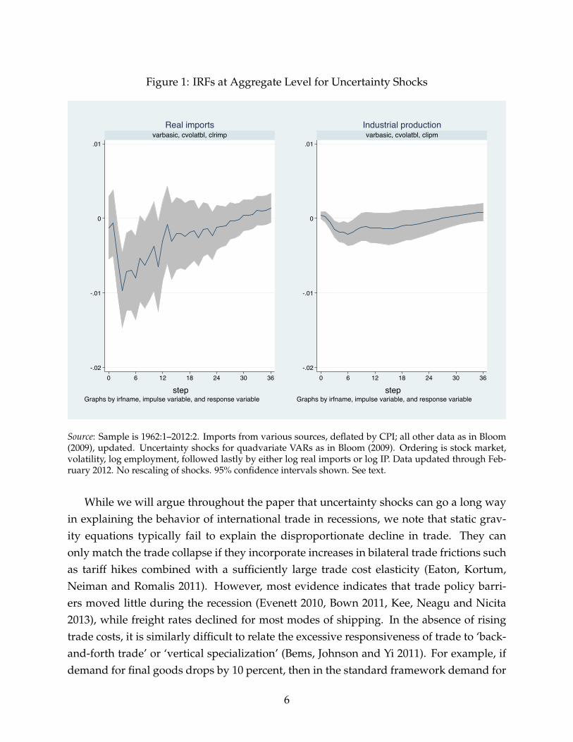
Figure 1: IRFs at Aggregate Level for Uncertainty Shocks

-.02

-.01

0

.01

0 6 12 18 24 30 36

varbasic, cvolatbl, clrimpReal imports

stepGraphs by irfname, impulse variable, and response variable

-.02

-.01

0

.01

0 6 12 18 24 30 36

varbasic, cvolatbl, clipmIndustrial production

stepGraphs by irfname, impulse variable, and response variable

Source: Sample is 1962:1–2012:2. Imports from various sources, deflated by CPI; all other data as in Bloom(2009), updated. Uncertainty shocks for quadvariate VARs as in Bloom (2009). Ordering is stock market,volatility, log employment, followed lastly by either log real imports or log IP. Data updated through Feb-ruary 2012. No rescaling of shocks. 95% confidence intervals shown. See text.

While we will argue throughout the paper that uncertainty shocks can go a long wayin explaining the behavior of international trade in recessions, we note that static grav-ity equations typically fail to explain the disproportionate decline in trade. They canonly match the trade collapse if they incorporate increases in bilateral trade frictions suchas tariff hikes combined with a sufficiently large trade cost elasticity (Eaton, Kortum,Neiman and Romalis 2011). However, most evidence indicates that trade policy barri-ers moved little during the recession (Evenett 2010, Bown 2011, Kee, Neagu and Nicita2013), while freight rates declined for most modes of shipping. In the absence of risingtrade costs, it is similarly difficult to relate the excessive responsiveness of trade to ‘back-and-forth trade’ or ‘vertical specialization’ (Bems, Johnson and Yi 2011). For example, ifdemand for final goods drops by 10 percent, then in the standard framework demand for

6

intermediates typically also drops by 10 percent throughout the supply chain.

3 A Model of Trade with Uncertainty Shocks

We build on Hassler’s (1996) setting of investment under uncertainty to construct a modelof trade in intermediate goods. Following the seminal contribution by Bloom (2009) wethen introduce second moment uncertainty shocks.

Hassler’s (1996) model starts from the well-established premise that uncertainty hasan adverse effect on investment. In our set-up we model ‘investment’ as firms’ investingin intermediate goods. Due to fixed costs of ordering firms build up an inventory ofintermediate goods that they run down over time and replenish at regular intervals. Theintermediate goods can be either ordered domestically or imported from abroad. Thus,we turn the model into an open economy.

In addition, firms face uncertainty over ‘business conditions,’ which means they ex-perience unexpected fluctuations in productivity and demand. What’s more, the degreeof uncertainty varies over time. Firms might therefore enjoy periods of calm when busi-ness conditions are relatively stable, or they might have to weather ‘uncertainty shocks’that lead to a volatile business environment characterized by large fluctuations. Over-all, this formulation allows us to model the link between production, international tradeand shifting degrees of uncertainty. Hassler’s (1996) key innovation is to formally modelhow changes in uncertainty influence investment. His model therefore serves as a naturalstarting point for our analysis of uncertainty shocks.

3.1 Production and Demand

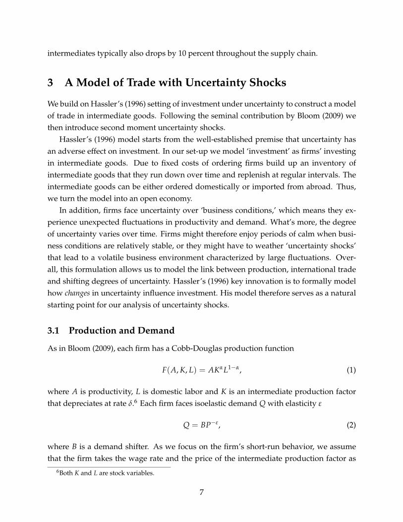
As in Bloom (2009), each firm has a Cobb-Douglas production function

F(A, K, L) = AKαL1−α, (1)

where A is productivity, L is domestic labor and K is an intermediate production factorthat depreciates at rate δ.6 Each firm faces isoelastic demand Q with elasticity ε

Q = BP−ε, (2)

where B is a demand shifter. As we focus on the firm’s short-run behavior, we assumethat the firm takes the wage rate and the price of the intermediate production factor as

6Both K and L are stock variables.

7

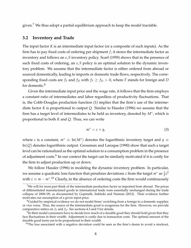
given.7 We thus adopt a partial equilibrium approach to keep the model tractable.

3.2 Inventory and Trade

The input factor K is an intermediate input factor (or a composite of such inputs). As thefirm has to pay fixed costs of ordering per shipment f , it stores the intermediate factor asinventory and follows an s, S inventory policy. Scarf (1959) shows that in the presence ofsuch fixed costs of ordering, an s, S policy is an optimal solution to the dynamic inven-tory problem. We assume that the intermediate factor is either ordered from abroad orsourced domestically, leading to imports or domestic trade flows, respectively. The corre-sponding fixed costs are fF and fD with fF ≥ fD > 0, where F stands for foreign and Dfor domestic.8

Given the intermediate input price and the wage rate, it follows that the firm employsa constant ratio of intermediates and labor regardless of productivity fluctuations. Thatis, the Cobb-Douglas production function (1) implies that the firm’s use of the interme-diate factor K is proportional to output Q. Similar to Hassler (1996) we assume that thefirm has a target level of intermediates to be held as inventory, denoted by M∗, which isproportional to both K and Q. Thus, we can write

m∗ = c+ q, (3)

where c is a constant, m∗ ≡ ln(M∗) denotes the logarithmic inventory target and q ≡ln(Q) denotes logarithmic output. Grossman and Laroque (1990) show that such a targetlevel can be rationalized as the optimal solution to a consumption problem in the presenceof adjustment costs.9 In our context the target can be similarly motivated if it is costly forthe firm to adjust production up or down.

We follow Hassler (1996) in modeling the dynamic inventory problem. In particular,we assume a quadratic loss function that penalizes deviations z from the target m∗ as 1

2 z2

with z ≡ m−m∗.10 Clearly, in the absence of ordering costs the firm would continuously

7We will for most part think of the intermediate production factor as imported from abroad. The pricesof differentiated manufactured goods in international trade were essentially unchanged during the tradecollapse of 2008/09, as documented by Gopinath, Itskhoki and Neiman (2012). Their evidence furthermotivates our assumption of a given input price.

8Guided by empirical evidence we do not model firms’ switching from a foreign to a domestic supplier,or vice versa. Thus, the source of the intermediate good is exogenous for the firm. However, we providecomparative statics on fF and fD. See sections 4.3 and 5 for details.

9In their model consumers have to decide how much of a durable good they should hold given that theyface fluctuations in their wealth. Adjustment is costly due to transaction costs. The optimal amount of thedurable good turns out to be proportional to their wealth.

10The loss associated with a negative deviation could be seen as the firm’s desire to avoid a stockout,

8

set m equal to the target m∗. However, since we assume positive ordering costs ( f >0), the firm faces a non-trivial trade-off as it needs to balance the fixed costs on the onehand and the costs of deviating from the target on the other. Imports are the changes ininventory brought about whenever the firm pays the fixed costs f to adjust m (assumingthat the intermediate input is sourced from abroad).

We solve for the optimal solution to this inventory problem subject to a stochasticprocess for output q. The optimal control solution can be characterized as follows: whenthe deviation of inventory z reaches a lower trigger point s, the firm orders the amount φ

so that the inventory rises to a return point of deviation S = s+ φ. Formally, we can statethe problem as

min{It,zt}∞

0

{E 0

∫ ∞

0e−rt

(12

z2t + It f

)d t}

(4)

subject to

z0 = z,

zt+d t =

{free if mt is adjusted,zt − δ d t− d q otherwise,

It d t =

{1 if mt is adjusted,0 otherwise.

It is a dummy variable that takes on the value 1 whenever the firm adjusts mt by payingf , r > 0 is a constant discount rate, and δ > 0 is the depreciation rate for the intermedi-ate so that d Kt/K = δ d t. Note that the intermediate input only depreciates if used inproduction, not if it is merely in storage as inventory.11

3.3 Business Conditions with Time-Varying Uncertainty

Due to market clearing output can move because of shifts in productivity A in equation(1) or demand shifts B in equation (2). Like Bloom (2009), we refer to the combinationof supply and demand shifters as business conditions. Specifically, we assume that outputq follows a stochastic marked point process that is known to the firm. With an instanta-

while the loss associated with a positive deviation could be interpreted as the firm’s desire to avoid exces-sive storage costs.

11In our trade and production data at the 4-digit industry level, examples of the intermediate factor Kinclude ‘electrical equipment’, ‘engines, turbines, and power transmission equipment’, ‘communicationsequipment’ and ‘railroad rolling stock.’ We can think of the firm described in our model as ordering a mixof such products. We therefore think of a situation where inventories are essentially a factor of production,for instance spare parts for when machines break down (Ramey 1989).

9

neous probability λ/2 per unit of time and λ > 0, q shifts up or down by the amountε:

qt+d t =

qt + ε with probability (λ/2)d t,qt with probability 1− λ d t,qt − ε with probability (λ/2)d t.

(5)

The shock ε can be interpreted as a sudden change in business conditions. Through theproportionality between output and the target level of inventory embedded in equation(3) a shift in q leads to an updated target inventory level m∗. Following Hassler (1996) weassume that ε is sufficiently large such that it becomes optimal for the firm to adjust m.12

That is, a positive shock to output increases m∗ sufficiently to lead to a negative deviationz that reaches below the lower trigger point s. As a result the firm restocks m. Vice versa,a negative shock reduces m∗ sufficiently such that z reaches above the upper trigger pointand the firm destocks m.13 Thus, to keep our model tractable we allow the firm to bothrestock and destock depending on the direction of the shock.

The arrival rate of shocks λ is the measure of uncertainty and thus a key parameter ofinterest. We interpret changes in λ as changes in the degree of uncertainty. Note that λ

determines the frequency of shocks, not the size of shocks. This feature is consistent withλ determining the second moment of shocks, not their first moment. More specifically,as the simplest possible set-up we follow Hassler (1996) by allowing uncertainty λω toswitch stochastically between two states ω ∈ {0, 1}: a state of low uncertainty λ0 and astate of high uncertainty λ1 with λ0 < λ1. The transition of the uncertainty states followsa Markov process

ωt+d t =

{ωt with probability 1− γω d t,ωt with probability γω d t,

(6)

where ωt = 1 if ωt = 0, and vice versa. The probability of switching the uncertainty statein the next instant d t is therefore γω d t, with the expected duration until the next switchgiven by γ−1

ω .Below we will choose parameter values for λ0, λ1, γ0 and γ1 that are consistent with

uncertainty fluctuations as observed over the past few decades.14 The firm knows the

12Hassler (1996, section 4) reports that relaxing the large shock assumption, while rendering the modelmore difficult to solve, appears to yield no qualitatively different results.

13To keep the exposition concise we do not explicitly describe the upper trigger here and focus on thelower trigger point s and the return point S. But it is straightforward to characterize the upper triggerpoint. See Hassler (1996) for details.

14Overall, the stochastic process for uncertainty is consistent with Bloom’s (2009). In his setting uncer-tainty also switches between two states (low and high uncertainty) with given transition probabilities. But

10

parameters of the stochastic process described by (5) and (6) and takes them into accountwhen solving its optimization problem (4).15

3.4 Solving the Inventory Problem

The Bellman equation for the inventory problem is

V(zt, ωt) =12

z2t d t+ (1− r d t)E tV(zt+d t, ωt+d t). (7)

The cost function V(zt, ωt) at time t in state ωt thus depends on the instantaneous losselement from the minimand (4), z2

t d t/2, as well as the discounted expected cost at timet+ d t. The second term can be further broken down as follows:

E tV(zt+d t, ωt+d t) =

Vz(zt, ωt)− δ d tVz(zt, ωt)

+λω d t {V(Sω, ωt) + f −V(zt, ωt)}+γω d t {V(zt, ωt)−V(zt, ωt)} ,

(8)

where Vz denotes the derivative of V with respect to z. The expected cost at time t+ d tthus takes into account the cost of depreciation over time through the term involving δ.It also captures the probability λω d t of a shock hitting the firm’s business conditions (inwhich case the firm would pay the ordering costs f to restock to its return point Sω), aswell as the probability γω d t that the uncertainty state switches from ωt to ωt.

Equations (7) and (8) form a system of two differential equations for the two possi-ble states ωt and ωt. Following Hassler (1996) we show in the technical appendix howstandard stochastic calculus techniques lead to a solution for the system. We have to usenumerical methods to obtain values for the four main endogenous variables of interest:the bounds s0 and S0 for the state of low uncertainty λ0, and the bounds s1 and S1 for thestate of high uncertainty λ1. It turns out that in either state, the cost function V reaches itslowest level at the respective return point Sω. This point represents the level of inventorythe firm ideally wants to hold given the expected outlook for business conditions andgiven it has just paid the fixed costs f for restocking.16

Following Hassler (1996) it can be shown that the following condition can be derived

he models uncertainty as the time variation of the volatility of a geometric random walk.15When we simulate the model in section 5, we consider a large number of firms that are identical apart

from receiving idiosyncratic shocks. Those firms do not behave strategically, and there are no self-fulfillingbouts of uncertainty.

16It would not be optimal for the firm to return to a point at which the cost function is above its minimum.The intuition is that in that case, the firm would on average spend less time in the lowest range of possiblecost values.

11

from the Bellman equation:17

12

(s2

ω − S2ω

)= (r+ λω) f + γω { f − (V(sω, ωt)−V(Sω, ωt))} > 0. (9)

This expression is strictly positive as (r+ λω) f > 0 and γω { f − (V(sω, ωt)−V(Sω, ωt))}≥ 0. This last non-negativity result holds because the smallest value of V can always bereached by paying the fixed costs f and stocking up to Sω. That is, for any zt, the costvalue V(zt, ωt) can never exceed the minimum value V(Sω, ωt) plus f . It therefore alsofollows that V(sω, ωt) can never exceed V(Sω, ωt) + f , i.e., V(sω, ωt) ≤ V(Sω, ωt) + f .

Recall that the lower trigger point sω is expressed as a deviation from the target levelm∗. We therefore have sω < 0. Conversely, the return point Sω is always positive, Sω > 0.The fact that expression (9) is positive implies |sω| > Sω, i.e., the lower trigger point isfurther from the target than the return point. Why does this asymmetry arise? Intuitively,in the absence of uncertainty the firm would stock as much inventory as to be at the targetvalue on average. That is, its inventory would be below and above the target exactly halfof the time, with the lower trigger point and return point equally distant from the target.However, in the presence of uncertainty this symmetry is no longer optimal. There isnow a positive probability that output q gets hit by a shock according to equation (5).Whenever a shock hits, the firm adjusts its inventory to the return point Sω.18 If thereturn point were the same distance from the target as the lower trigger point, the firm’sinventory would on average be above target. To avoid this imbalance the firm chooses areturn point that is relatively close to the target.19

4 Time-Varying Uncertainty and Inventory Behavior

The main purpose of this section is to explore how the firm endogenously changes its s, Sbounds in response to increased uncertainty. Our key result is that the firm lowers thebounds in response to increased uncertainty. In addition, we are interested in compara-tive statics for the depreciation rate δ and the fixed cost of ordering f . As explained inthe preceding section, the model cannot be solved analytically. Instead, we use numericalmethods.

17For details of the derivation see Hassler (1996, Appendix 2).18Recall from section 3.3 that for tractability the shock ε is assumed to be sufficiently large.19Although we will fill in more details in section 4, we can refer interested readers to Figure 5 where we

illustrate the difference between no uncertainty (cases 1 and 2) and positive uncertainty (cases 3a and 3b).

12

4.1 Parameterizing the Model

We choose the same parameter values for the interest rate and rate of depreciation as inBloom (2009), i.e., r = 0.065 and δ = 0.1 per year. The interest rate value corresponds tothe long-run average for the U.S. firm-level discount rate. Based on data for the U.S. man-ufacturing sector over the period from 1960 to 1988, Nadiri and Prucha (1996) estimatedepreciation rates of 0.059 for physical capital and 0.12 for R&D capital. As reported intheir paper, those are somewhat lower than estimates by other authors. We therefore takeδ = 0.1 as a reasonable baseline value.

For the stochastic uncertainty process described by equations (5) and (6) we chooseparameter values that are consistent with Bloom’s (2009) data on stock market volatility.In his Table II he reports that an uncertainty shock has an average half-life of two months.This information can be expressed in terms of the transition probabilities in equation (6)with the help of a standard process of exponential decay for a quantity Dt:

Dt = D0 exp(−gt).

Setting t equal to 2/12 years yields a rate of decay g = 4.1588 for Dt to halve. Thedecaying quantity Dt in that process can be thought of as the number of discrete elementsin a certain set. We can then compute the average length of time that an element remainsin the set. This is the mean lifetime of the decaying quantity, and it is simply given byg−1. It corresponds to the expected duration of the high-uncertainty state, γ−1

1 , so thatγ1 = g = 4.1588. Thus, the average duration of the high-uncertainty period follows as4.1588−1 = 0.2404 years.

Bloom (2009) furthermore reports 17 uncertainty shocks in 46 years. Hence, an un-certainty shock arrives on average every 46/17 = 2.7059 years. Given the duration ofhigh-uncertainty periods from above, this implies an average duration of low-uncertaintyperiods of 2.7059− 0.2404 = 2.4655 years. It follows γ0 = 2.4655−1 = 0.4056.

The uncertainty term λ d t in the marked point process (5) indicates the probabilitythat output is hit in the next instant by a supply or demand shock that is sufficiently largeto shift the target level of inventory. Thus, the expected length of time until the next shockis λ−1. It is difficult to come up with an empirical counterpart of the frequency of suchshocks since they are unobserved. For the baseline level of uncertainty we set λ0 = 1,which implies that the target level of inventory is adjusted on average once a year. Thisvalue can therefore be interpreted as an annual review of inventory policy. However, wenote that our results are not very sensitive to the λ0 value. In our baseline specification wefollow Bloom (2009, Table II) by doubling the standard deviation of business conditions in

13

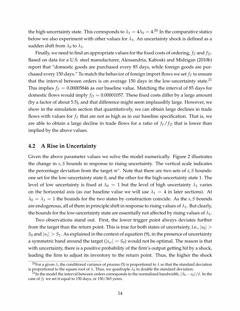
the high-uncertainty state. This corresponds to λ1 = 4λ0 = 4.20 In the comparative staticsbelow we also experiment with other values for λ1. An uncertainty shock is defined as asudden shift from λ0 to λ1.

Finally, we need to find an appropriate values for the fixed costs of ordering, fF and fD.Based on data for a U.S. steel manufacturer, Alessandria, Kaboski and Midrigan (2010b)report that “domestic goods are purchased every 85 days, while foreign goods are pur-chased every 150 days.” To match the behavior of foreign import flows we set fF to ensurethat the interval between orders is on average 150 days in the low-uncertainty state.21

This implies fF = 0.00005846 as our baseline value. Matching the interval of 85 days fordomestic flows would imply fD = 0.00001057. These fixed costs differ by a large amount(by a factor of about 5.5), and that difference might seem implausibly large. However, weshow in the simulation section that quantitatively, we can obtain large declines in tradeflows with values for fF that are not as high as in our baseline specification. That is, weare able to obtain a large decline in trade flows for a ratio of fF/ fD that is lower thanimplied by the above values.

4.2 A Rise in Uncertainty

Given the above parameter values we solve the model numerically. Figure 2 illustratesthe change in s, S bounds in response to rising uncertainty. The vertical scale indicatesthe percentage deviation from the target m∗. Note that there are two sets of s, S bounds:one set for the low-uncertainty state 0, and the other for the high-uncertainty state 1. Thelevel of low uncertainty is fixed at λ0 = 1 but the level of high uncertainty λ1 varieson the horizontal axis (as our baseline value we will use λ1 = 4 in later sections). Atλ0 = λ1 = 1 the bounds for the two states by construction coincide. As the s, S boundsare endogenous, all of them in principle shift in response to rising values of λ1. But clearly,the bounds for the low-uncertainty state are essentially not affected by rising values of λ1.

Two observations stand out. First, the lower trigger point always deviates furtherfrom the target than the return point. This is true for both states of uncertainty, i.e., |s0| >S0 and |s1| > S1. As explained in the context of equation (9), in the presence of uncertaintya symmetric band around the target (|sω| = S0) would not be optimal. The reason is thatwith uncertainty, there is a positive probability of the firm’s output getting hit by a shock,leading the firm to adjust its inventory to the return point. Thus, the higher the shock

20For a given λ, the conditional variance of process (5) is proportional to λ so that the standard deviationis proportional to the square root of λ. Thus, we quadruple λ0 to double the standard deviation.

21In the model the interval between orders corresponds to the normalized bandwidth, (S0− s0)/δ. In thecase of fF we set it equal to 150 days, or 150/365 years.

14

Figure 2: Change in s, S bounds due to higher uncertainty. The low-uncertainty state is ingrey, the high-uncertainty state is in black.

probability, the more the firm would stock inventory above target. To counteract thistendency it is optimal for the firm to set the return point closer to the target than thelower trigger point.

Second, the bounds for the high-uncertainty state decrease with the extent of uncer-tainty, i.e., ∂S1/∂λ1 < 0 and ∂s1/∂λ1 < 0. The intuition for the drop in the return pointS1 is the same as above – increasing uncertainty means more frequent adjustment so thatS1 needs to be lowered to avoid excessive inventory holdings. The intuition for the dropin the lower trigger point s1 reflects the rising option value of waiting. Suppose the firmis facing low inventory and decides to pay the fixed costs of ordering f to stock up. If thefirm gets hit by a shock in the next instant, it would have to pay f again. The firm couldhave therefore saved one round of fixed costs by waiting. Waiting longer corresponds toa lower value of s1. This logic follows immediately from the literature on uncertainty andthe option value of waiting (McDonald and Siegel 1986, Dixit 1989, Pindyck 1991).

Figure 3 shows that the decline in the lower trigger point s1 compared to s0 can be quitesubstantial for high degrees of uncertainty. It plots the percentage decline in s1 relativeto s0. Given the above parameterization, the lower trigger point declines by 28 percentwhen uncertainty increases to λ1 = 4 from λ0 = 1. As we show in section 5 when wesimulate the model, this translates into a precipitous drop of imports. Intuitively, whenuncertainty rises, the firm becomes more cautious and adopts a wait-and-see attitude. Itruns down its inventory further than in the low-uncertainty state, and it does not stock up

15

Figure 3: How uncertainty decreases the lower trigger point (compared to the low-uncertainty state).

as much. It turns out that the firm lowers s1 more than S1 so that the bandwidth (S1− s1)

rises in response to higher uncertainty. Figure 4 plots this increase in bandwidth.Figure 5 summarizes the main qualitative results in a compact way. Case 1 depicts the

(hypothetical) situation where both fixed costs f and uncertainty λ are negligible. Due tothe very low fixed costs the bandwidth (i.e., the height of the box) is tiny, and due to thelack of uncertainty the s1 and S1 bounds are essentially symmetric around the target levelm∗. In case 2 the fixed costs become larger, which pushes both s1 and S1 further awayfrom the target but in a symmetric way. Cases 3a and 3b correspond to the situation weconsider in this paper with non-negligible degrees of uncertainty as in Figures 2–4. Theuncertainty in case 3a induces two effects compared to case 2. First, both s1 and S1 shiftdown so that they are no longer symmetric around the target. Second, the bandwidthincreases further (see Figure 4). A shift to even more uncertainty (case 3b) reinforcesthese two effects.

4.3 Comparative Statics

4.3.1 Varying the Fixed Costs of Ordering

We expect fixed costs of ordering to be lower when the intermediate input is ordereddomestically, i.e., fD < fF. Figure 6 shows the effect of using the value fD from abovethat corresponds to an average interval of 85 days between domestic orders compared to

16

Figure 4: How uncertainty increases the s, S bandwidth (compared to the low-uncertaintystate).

Figure 5: Summary: How uncertainty pushes down the s, S bounds and increases thebandwidth.

m = ln(M)

m* s1

S1

s2

S2

s3a

S3a

Case 1:

𝑓 → 0 λ → 0

Case 2:

𝑓 > 0 λ → 0

Case 3a:

𝑓 > 0 λ > 0

Case 3b:

𝑓 > 0 λ ≫ 0

S3b

s3b

17

Figure 6: The effect of a lower fixed costs of ordering on the decrease in the lower triggerpoint.

the baseline value fF in Figure 3. Lower fixed costs imply more frequent ordering andtherefore allow the firm to keep its inventory closer to the target level. This means thatfor any given level of uncertainty, the optimal lower trigger point does not deviate as farfrom the target compared to the high fixed cost scenario.

4.3.2 Varying the Depreciation Rate

Some types of imports are inherently difficult to store as inventory, for instance food prod-ucts and other perishable goods. We model this inherent difference in storability with ahigher rate of depreciation of δ = 0.2 compared to the baseline value of δ = 0.1. In gen-eral, the larger the depreciation rate, the smaller the decreases in the lower trigger pointand the return point in response to heightened uncertainty. Intuitively, with a largerdepreciation rate the firm orders more frequently. The value of waiting is therefore di-minished. Figure 7 graphs the percentage decline in the lower trigger point s1 relative tos0 for both the baseline depreciation rate (as in Figure 3) and the higher value.

5 Simulating an Uncertainty Shock

So far we have described the behavior of a single firm. We now simulate 50,000 firms thatreceive shocks according to the stochastic uncertainty process in equations (5) and (6).

18

Figure 7: The effect of a higher depreciation rate on the decrease in the lower trigger point.

These shocks are idiosyncratic for each firm but drawn from the same distribution. Thefirms are identical in all other respects. We use the same parameter values as in section4.1.

We should add that we do not model an extensive margin response, i.e., firms nei-ther enter nor exit over the simulation period.22 This approach seems reasonable giventhat most of the changes in the value of international trade during the trade collapseof 2008/09 happened at the intensive margin (see Behrens, Corcos and Mion 2013 andBricongne et al. 2012). Allowing for extensive margin responses would be an importantavenue for future research. We conjecture that the extensive margin would amplify un-certainty shocks. Firms would likely exit in the face of higher uncertainty and enter oncethe recovery takes hold, thus reinforcing the effects of higher uncertainty.

5.1 A Permanent Uncertainty Shock

We simulate a uncertainty shock by permanently shifting the economy from low uncer-tainty λ0 to high uncertainty λ1. A key result from section 4.2 is that firms lower their s, Sbounds in response to increased uncertainty. This shift leads to a sharp downward adjust-ment of aggregate intermediate input inventories and thus a decline in imports. Figure8 plots the aggregate imports of intermediate goods in the economy (normalized to 1 forthe average value). Given our parameterization imports decrease by about 25 percent in

22Neither do we model firms’ switching from a foreign to a domestic supplier, or vice versa.

19

Figure 8: Simulating the response of aggregate imports to an uncertainty shock.

−1 0 1 2 30.3

0.4

0.5

0.6

0.7

0.8

0.9

1

1.1

1.2

1.3

1.4

1.5

Months after shock

Agg

rega

te im

port

s(n

orm

aliz

ed to

1 fo

r av

erag

e)

response to the shock. The decrease happens quickly within about one month, followedby a quick discovery and in fact an overshoot (we comment on the overshoot below).As in Bloom (2009), this pattern of sharp contraction and strong recovery is typical foruncertainty shocks.

While the trade collapse and recovery happen quickly in the simulation, this processtakes longer in the data. For instance, during the Great Recession German imports peakedin the second quarter of 2008, rapidly declined by 32 percent and only returned to theirprevious level by the third quarter of 2011.23 Such persistence could be introduced intoour simulation by staggering firms’ responses. Currently, all firms perceive uncertaintyin exactly the same way and thus synchronize their reactions. It might be more realisticto introduce some degree of heterogeneity by allowing firms to react at slightly differenttimes. In particular, firms might have different assessments as to the time when uncer-tainty has faded and business conditions have normalized. This would tend to stretchout the recovery of trade. Moreover, delivery lags could be introduced that vary acrossindustries. We abstracted from such extensions here in order to keep the model tractable.

23Most high-income countries experienced similar patterns. U.S. and Japanese imports declined by 38percent and 40 percent over that period, respectively. Data source: International Monetary Fund, Directionof Trade Statistics.

20

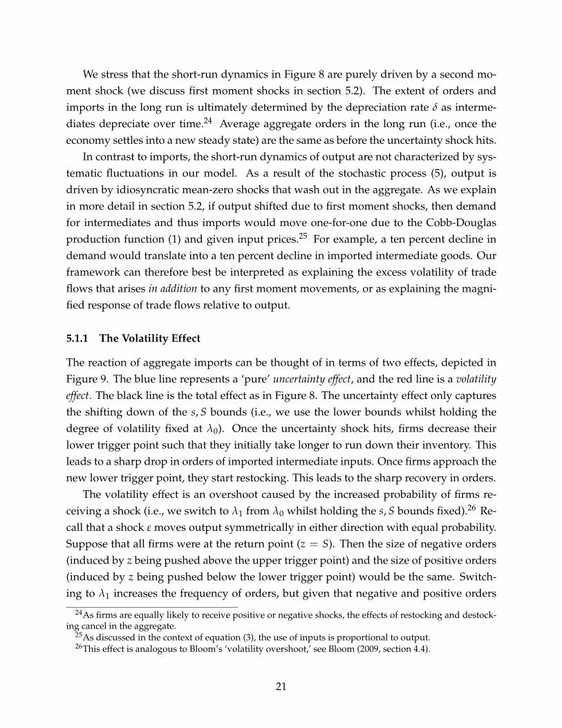
We stress that the short-run dynamics in Figure 8 are purely driven by a second mo-ment shock (we discuss first moment shocks in section 5.2). The extent of orders andimports in the long run is ultimately determined by the depreciation rate δ as interme-diates depreciate over time.24 Average aggregate orders in the long run (i.e., once theeconomy settles into a new steady state) are the same as before the uncertainty shock hits.

In contrast to imports, the short-run dynamics of output are not characterized by sys-tematic fluctuations in our model. As a result of the stochastic process (5), output isdriven by idiosyncratic mean-zero shocks that wash out in the aggregate. As we explainin more detail in section 5.2, if output shifted due to first moment shocks, then demandfor intermediates and thus imports would move one-for-one due to the Cobb-Douglasproduction function (1) and given input prices.25 For example, a ten percent decline indemand would translate into a ten percent decline in imported intermediate goods. Ourframework can therefore best be interpreted as explaining the excess volatility of tradeflows that arises in addition to any first moment movements, or as explaining the magni-fied response of trade flows relative to output.

5.1.1 The Volatility Effect

The reaction of aggregate imports can be thought of in terms of two effects, depicted inFigure 9. The blue line represents a ‘pure’ uncertainty effect, and the red line is a volatilityeffect. The black line is the total effect as in Figure 8. The uncertainty effect only capturesthe shifting down of the s, S bounds (i.e., we use the lower bounds whilst holding thedegree of volatility fixed at λ0). Once the uncertainty shock hits, firms decrease theirlower trigger point such that they initially take longer to run down their inventory. Thisleads to a sharp drop in orders of imported intermediate inputs. Once firms approach thenew lower trigger point, they start restocking. This leads to the sharp recovery in orders.

The volatility effect is an overshoot caused by the increased probability of firms re-ceiving a shock (i.e., we switch to λ1 from λ0 whilst holding the s, S bounds fixed).26 Re-call that a shock ε moves output symmetrically in either direction with equal probability.Suppose that all firms were at the return point (z = S). Then the size of negative orders(induced by z being pushed above the upper trigger point) and the size of positive orders(induced by z being pushed below the lower trigger point) would be the same. Switch-ing to λ1 increases the frequency of orders, but given that negative and positive orders

24As firms are equally likely to receive positive or negative shocks, the effects of restocking and destock-ing cancel in the aggregate.

25As discussed in the context of equation (3), the use of inputs is proportional to output.26This effect is analogous to Bloom’s ‘volatility overshoot,’ see Bloom (2009, section 4.4).

21

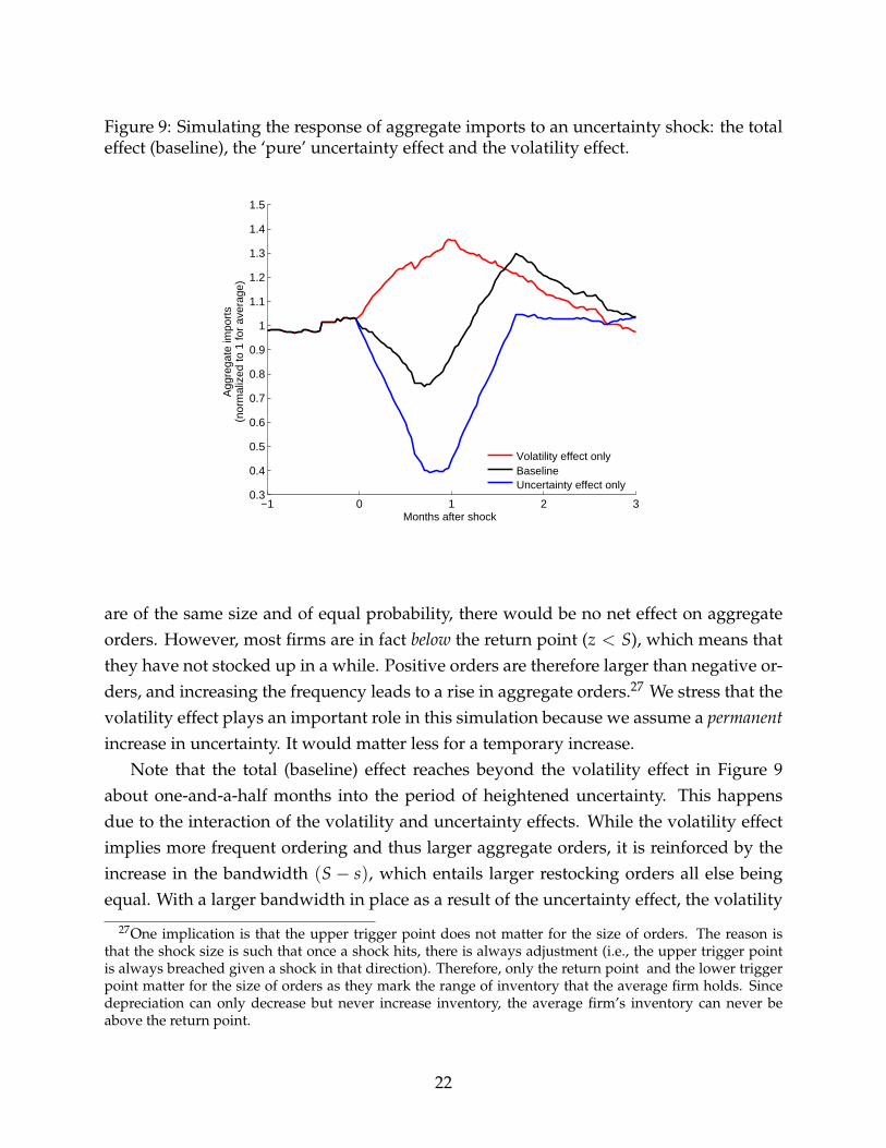
Figure 9: Simulating the response of aggregate imports to an uncertainty shock: the totaleffect (baseline), the ‘pure’ uncertainty effect and the volatility effect.

−1 0 1 2 30.3

0.4

0.5

0.6

0.7

0.8

0.9

1

1.1

1.2

1.3

1.4

1.5

Months after shock

Agg

rega

te im

port

s(n

orm

aliz

ed to

1 fo

r av

erag

e)

Volatility effect onlyBaselineUncertainty effect only

are of the same size and of equal probability, there would be no net effect on aggregateorders. However, most firms are in fact below the return point (z < S), which means thatthey have not stocked up in a while. Positive orders are therefore larger than negative or-ders, and increasing the frequency leads to a rise in aggregate orders.27 We stress that thevolatility effect plays an important role in this simulation because we assume a permanentincrease in uncertainty. It would matter less for a temporary increase.

Note that the total (baseline) effect reaches beyond the volatility effect in Figure 9about one-and-a-half months into the period of heightened uncertainty. This happensdue to the interaction of the volatility and uncertainty effects. While the volatility effectimplies more frequent ordering and thus larger aggregate orders, it is reinforced by theincrease in the bandwidth (S − s), which entails larger restocking orders all else beingequal. With a larger bandwidth in place as a result of the uncertainty effect, the volatility

27One implication is that the upper trigger point does not matter for the size of orders. The reason isthat the shock size is such that once a shock hits, there is always adjustment (i.e., the upper trigger pointis always breached given a shock in that direction). Therefore, only the return point and the lower triggerpoint matter for the size of orders as they mark the range of inventory that the average firm holds. Sincedepreciation can only decrease but never increase inventory, the average firm’s inventory can never beabove the return point.

22

Figure 10: Simulating the inventory position of the average firm.

−1 0 1 2 3−5

−4

−3

−2

−1

0

1

2

3

4x 10

−3

Months after shock

Dev

iatio

n of

impo

rted

inte

rmed

iate

sfr

om ta

rget

leve

l for

ave

rage

firm

effect is in fact stronger compared to the scenario with no interaction as indicated by thered line.

In Figure 10 we illustrate the inventory position of the average firm. Specifically, weplot the average deviation of imported intermediates from the target level. In the steadystate before the uncertainty shock hits, this deviation is essentially zero as firms on aver-age hold precisely the amount of inventory that minimizes their loss function. After theshock has hit, their average inventories initially decline sharply as firms decrease theirlower trigger point. This is driven by the uncertainty effect described above. But at thesame time, the higher volatility means that firms are more likely to restock, implying arising average deviation over time. Although this volatility effect sets in immediately, itis initially dominated by the uncertainty effect. In Figure 10 firms’ inventories eventuallystart rising after just under a month into the period of heightened uncertainty.

5.1.2 Comparative Statics

In Figure 11 we plot the total effect of an uncertainty shock for three different values offixed costs fF. The black line corresponds to the baseline value of fF = 0.00005846. Theremaining two lines in grey correspond to smaller values of fF. Their values are fF =

23

Figure 11: Simulating aggregate imports with different values of fixed costs of ordering.

−1 0 1 2 30.3

0.4

0.5

0.6

0.7

0.8

0.9

1

1.1

1.2

1.3

1.4

1.5

Months after shock

Agg

rega

te im

port

s(n

orm

aliz

ed to

1 fo

r av

erag

e)

0.00004846 for the dark grey line and fF = 0.00003846 for the light grey line. Althoughthe latter value is about a third smaller than the baseline value, imports still drop by over20 percent (compared to 25 percent in the baseline scenario).

The insight is that although the trade collapse becomes less severe with smaller fixedcost values (as predicted by the theory), quantitatively the collapse is not as sensitive tofixed costs above a certain threshold. Thus, we do have to rely on fF being substantiallylarger than fD to generate a strong decline in international trade. In case of the lightgrey line in Figure 11, the foreign fixed cost value is only about 3.6 times as large asthe domestic fixed cost value ( fD = 0.00001057 in section 4.1 so that fF/ fD = 3.64).In contrast, Alessandria, Kaboski and Midrigan (2010a) use a ratio of fF/ fD = 6.54.28

The reason that smaller and arguably more plausible values of fF suffice is as follows.The decline of the lower trigger point in response to an uncertainty shock (as depictedin Figure 6) is increasing but concave in fF. Thus, increases in fF have a strong marginalimpact when fF is low. Once fF is high, increases have a weak impact on the lower triggerpoint. For instance, the impact associated with the baseline value of fF makes up more

28In their benchmark case, Alessandria, Kaboski and Midrigan (2010a, Table 4) choose values for the fixedcosts of ordering that correspond to 23.88 percent of mean revenues for foreign orders and 3.65 percent ofmean revenues for domestic orders.

24

Figure 12: Simulating aggregate imports with different values of the depreciation rate.

−1 0 1 2 30.3

0.4

0.5

0.6

0.7

0.8

0.9

1

1.1

1.2

1.3

1.4

1.5

Months after shock

Agg

rega

te im

port

s(n

orm

aliz

ed to

1 fo

r av

erag

e)

than two-thirds (72 percent) of the impact associated with doubling fF.29

In Figure 12 we plot the effect of an uncertainty shock for three different values of thedepreciation rate δ. The black line is for our baseline value of δ = 0.10. The dark greyline corresponds to δ = 0.125 and the light grey line is for δ = 0.15. As predicted by thetheory, higher rates of depreciation tend to entail a smaller adjustment of s, S bands sothat the decline in imports is not as pronounced.

5.2 A First Moment Shock

In section 5.1 we only consider a second moment shock. Whereas aggregate imports dis-play distinct short-run dynamics, aggregate output is flat because positive and negativeshocks at the firm level are of equal probability and thus exactly offset each other. Theincrease in volatility due to the second moment shock does not change this result.

We now consider a first moment shock. Due to the Cobb-Douglas production function(1) and due to the assumption of fixed input prices, it follows that the optimal ratios ofthe production factors to output, K/Q and L/Q, do not vary over time in our model. At

29Given the parameterization in section 4.1, the baseline value of fF = 0.00005846 is associated with adecline in the lower trigger point by 27.7 percent in response to an uncertainty shock. Doubling the baselinevalue of fF is associated with a 38.4 percent decline. It follows 27.7/38.4 = 0.72.

25

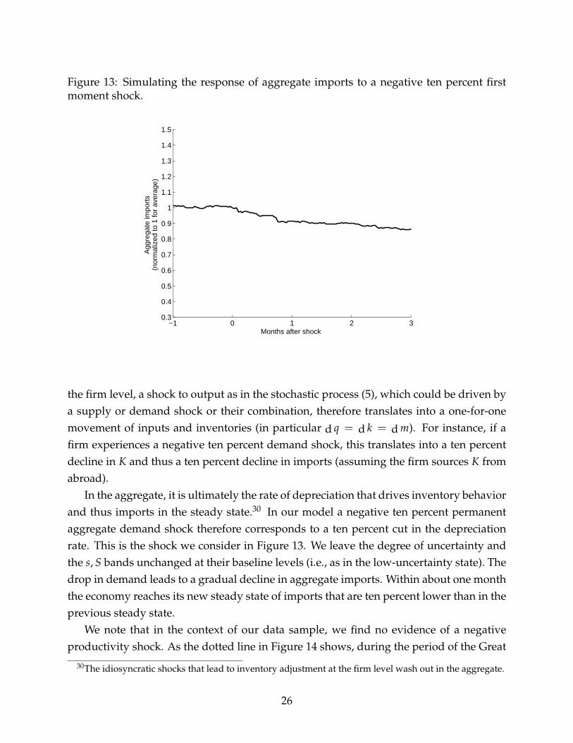
Figure 13: Simulating the response of aggregate imports to a negative ten percent firstmoment shock.

−1 0 1 2 30.3

0.4

0.5

0.6

0.7

0.8

0.9

1

1.1

1.2

1.3

1.4

1.5

Months after shock

Agg

rega

te im

port

s(n

orm

aliz

ed to

1 fo

r av

erag

e)

the firm level, a shock to output as in the stochastic process (5), which could be driven bya supply or demand shock or their combination, therefore translates into a one-for-onemovement of inputs and inventories (in particular d q = d k = d m). For instance, if afirm experiences a negative ten percent demand shock, this translates into a ten percentdecline in K and thus a ten percent decline in imports (assuming the firm sources K fromabroad).

In the aggregate, it is ultimately the rate of depreciation that drives inventory behaviorand thus imports in the steady state.30 In our model a negative ten percent permanentaggregate demand shock therefore corresponds to a ten percent cut in the depreciationrate. This is the shock we consider in Figure 13. We leave the degree of uncertainty andthe s, S bands unchanged at their baseline levels (i.e., as in the low-uncertainty state). Thedrop in demand leads to a gradual decline in aggregate imports. Within about one monththe economy reaches its new steady state of imports that are ten percent lower than in theprevious steady state.

We note that in the context of our data sample, we find no evidence of a negativeproductivity shock. As the dotted line in Figure 14 shows, during the period of the Great

30The idiosyncratic shocks that lead to inventory adjustment at the firm level wash out in the aggregate.

26

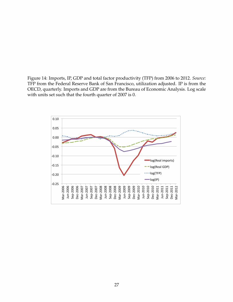
Figure 14: Imports, IP, GDP and total factor productivity (TFP) from 2006 to 2012. Source:TFP from the Federal Reserve Bank of San Francisco, utilization adjusted. IP is from theOECD, quarterly. Imports and GDP are from the Bureau of Economic Analysis. Log scalewith units set such that the fourth quarter of 2007 is 0.

-­‐0.25  

-­‐0.20  

-­‐0.15  

-­‐0.10  

-­‐0.05  

0.00  

0.05  

0.10  

Mar-­‐2006  

Jun-­‐2006  

Sep-­‐2006  

Dec-­‐20

06  

Mar-­‐2007  

Jun-­‐2007  

Sep-­‐2007  

Dec-­‐20

07  

Mar-­‐2008  

Jun-­‐2008  

Sep-­‐2008  

Dec-­‐20

08  

Mar-­‐2009  

Jun-­‐2009  

Sep-­‐2009  

Dec-­‐20

09  

Mar-­‐2010  

Jun-­‐2010  

Sep-­‐2010  

Dec-­‐20

10  

Mar-­‐2011  

Jun-­‐2011  

Sep-­‐2011  

Dec-­‐20

11  

Mar-­‐2012  

log(Real  imports)  

log(Real  GDP)  

log(TFP)  

log(IP)  

27

Trade Collapse total factor productivity in fact increased. A negative first moment shockto demand would go in the right direction but in our framework would not be sufficientto account for the severity of the trade collapse.

Alessandria, Kaboski and Midrigan (2010a) also develop an s, S inventory model witha band of inaction as in our model. However, they only consider first moment shocks (inparticular a negative supply shock) but no second moment shocks. In contrast to Figure13, their model nevertheless generates a decline in imports that exceeds the decline inoutput or sales. The reason is that they treat the intermediate input as a flow variable thatneeds to be replaced fully every period, and that the firm has a desired inventory-to-salesratio above 1. Once sales take a hit, a multiplier effect kicks in such that imports are re-duced more than one-for-one because firms run down their high levels of inventory. Inour model, however, the imported input factor is not fully absorbed in the productionprocess. It only depreciates by rate δ, which is less than 100 percent in our parameteriza-tion. We do not impose a desired inventory-to-sales ratio above 1. Instead, we generate adisproportionate decline in imports through an endogenous adjustment of s, S inventorybands caused by a second moment shock.

6 Empirical Evidence

To explore the relationship between uncertainty, production, and international trade werun vector autoregressions (VARs) with U.S. data. In particular, we follow the seminalwork of Bloom (2009) in running a VAR to generate an impulse response function (IRF)relating the reactions of key model quantities, in this case not only industrial productionbut also imports, to the underlying impulses which take the form of shocks to uncertainty.

We contend that, as with the application to production volatility, the payoffs to anuncertainty-based approach will turn out to be substantial again in the new setting wepropose for modeling trade volatility. Recall that in the view of Bloom (2009, p. 627):

More generally, the framework in this paper also provides one response tothe “where are the negative productivity shocks?” critique of real businesscycle theories. In particular, since second-moment shocks generate large fallsin output, employment, and productivity growth, it provides an alternativemechanism to first-moment shocks for generating recessions.

The same might then be said of theories of trade collapse that rely on negative pro-ductivity shocks, or other first moment shocks. So by the same token, the framework in

28

our paper provides one response to the “where are the increases in trade frictions?” ob-jection that is often cited when standard static models are unable to otherwise explain theamplified nature of trade collapses in recessions, relative to declines in output. Our theo-retical model, and empirical evidence, can thus be seamlessly integrated with the Bloom(2009) view of uncertainty-driven recessions, whilst matching one other crucial and re-current feature of international economic experience: the highly magnified volatility oftrade, which has been a focus of inquiry since at least the 1930s, and which, since the on-set of the Great Recession has flared again as an object of curiosity and worry to scholarsand policymakers alike.

6.1 Four Testable Hypotheses

To look ahead and quickly sum up the bottom line, our empirical results expose severalnew and important stylized facts, all of which are consistent with, and thus can motivateour previously described theoretical framework. Specifically we focus on testing fourempirical propositions that would be implied by our theory.

• First, trade volumes do respond to uncertainty shocks, the effects are quantitativelyand statistically significant, and are robust to different samples and methods. Inaddition, trade volumes respond much more to uncertainty shocks than does thevolume of industrial production; that is to say, there is something fundamentallydifferent about the dynamics of traded goods supplied via the import channel, ascompared to supply originating from domestic industrial production.

• Second, we confirm that these findings are true not just at the aggregate level, butalso at the disaggregated level, indicating that the amplified dynamic response oftraded goods is not just a sectoral composition effect.

• Third, we find that the dynamic response of traded goods to uncertainty shocks isgreatest in durable goods sectors as compared to nondurable goods sectors, con-sistent with the theoretical model where a decrease in the depreciation parameter(interpreted as a decrease in perishability) leads to a larger response.

• Fourth, we find corroborative evidence in the response of aggregate input invento-ries to uncertainty shocks, and in the stronger response of imports to uncertaintyshocks in those sectors where a larger share of the product is used downstream asan intermediate input.

29

The following parts of this section are structured as follows. The first part brieflyspells out the empirical VAR methods we employ based on Bloom (2009). The secondpart spells out the data we have at our disposal, some of it newly collected, to examine thedifferences between trade and industrial production in this framework. The subsequentparts discuss our findings on the first three testable hypotheses noted above, and wediscuss the corroborative evidence in the next section, before concluding.

6.2 Computing the Responses to an Uncertainty Shock

In typical business cycle empirical work, researchers are often interested in the responseof key variables, most of all output, to various shocks, most often a shock to the levelof technology or productivity. The analysis of such first moment shocks has long been acenterpiece of the macroeconomic VAR literature. The innovation of Bloom (2009) was toconstruct, simulate and empirically estimate a model where the key shock of interest is asecond moment shock, which is conceived of as an ‘uncertainty shock’ of a specific form.This shock amounts to an increase in the variance, but not the mean, of a composite ‘busi-ness condition’ disturbance in the model, which can be flexibly interpreted as a demandor supply shock. For empirical purposes when the model is estimated using data on thepostwar U.S., Bloom proposes that changes in the market price of the VXO index, a dailyoptions-based implied stock market volatility for a 30-day horizon, be used as a proxy forthe uncertainty shock, with realized volatility used when the VXO is not available. A plotof this series, scaled to an annualized form, and extended to 2012, is shown in Figure 15.31

Following Bloom (2009) we evaluate the impact of uncertainty shocks using VARson monthly data from June 1962 (the same as in Bloom) to February 2012 (going be-yond Bloom’s end date of June 2008). Bloom’s full set of variables, in VAR estimationorder are as follows: log(S&P500 stock market index), stock-market volatility indica-tor, Federal Funds Rate, log(average hourly earnings), log(consumer price index), hours,log(employment), and log(industrial production).32

31As Bloom (2009, Figure 1) notes: “Pre-1986 the VXO index is unavailable, so actual monthly returnsvolatilities are calculated as the monthly standard deviation of the daily S&P500 index normalized to thesame mean and variance as the VXO index when they overlap from 1986 onward. Actual and VXO arecorrelated at 0.874 over this period. A brief description of the nature and exact timing of every shockis contained in the empirical appendix [in progress]. The asterisks indicate that for scaling purposes themonthly VXO was capped at 50. Uncapped values for the Black Monday peak are 58.2 and for the creditcrunch peak are 64.4. LTCM is Long Term Capital Management.” For comparability, we follow exactly thesame definitions here and we thank Nicholas Bloom for providing us with an updated series extended to2012.

32In terms of VAR variable ordering and variable definitions we follow Bloom (2009) exactly for compa-rability. As Bloom notes: “This ordering is based on the assumptions that shocks instantaneously influencethe stock market (levels and volatility), then prices (wages, the consumer price index (CPI), and interest

30

Figure 15: The Bloom (2009) Index: Monthly U.S. stock market volatility, 1962–201210

10

1020

20

2030

30

3040

40

4050

50

50Uncertainty index (annualized standard deviation, %)

Unce

rtai

nty

inde

x (a

nnua

lized

sta

ndar

d de

viat

ion,

%)

Uncertainty index (annualized standard deviation, %)1960

1960

19601970

1970

19701980

1980

19801990

1990

19902000

2000

20002010

2010

2010

Source: Bloom (2009) and personal correspondence. See footnote 31.

For simplicity, for the main results of this paper presented in this section, all VARs ofthis form are estimated using a quad-variate VAR (log stock-market levels, the volatilityindicator, log employment, and lastly the industrial production or trade indicator).

6.3 Data

Many of our key variables are taken from the exact same sources as Bloom (2009). As itis noted: “The full set of VAR variables in the estimation are log industrial production inmanufacturing (Federal Reserve Board of Governors, seasonally adjusted), employmentin manufacturing (BLS, seasonally adjusted), average hours in manufacturing (BLS, sea-sonally adjusted), log consumer price index (all urban consumers, seasonally adjusted),log average hourly earnings for production workers (manufacturing), Federal Funds rate(effective rate, Federal Reserve Board of Governors), a monthly stock-market volatilityindicator (described below)[above here], and the log of the S&P500 stock-market index.

rates), and finally quantities (hours, employment, and output). Including the stock-market levels as thefirst variable in the VAR ensures the impact of stock-market levels is already controlled for when lookingat the impact of volatility shocks.”

31

All variables are HP detrended using a filter value of λ = 129, 600.” We follow thesedefinitions exactly.

However, in some key respects, our data requirement are much larger than this. Forstarters, we are interested in assessing the response of trade, so we needed to collectmonthly import volume data. In addition, we are interested in computing disaggregatedresponses of trade and industrial production (IP) in different sectors, in the aftermathof uncertainty shocks, in an attempt to gauge whether some of the key predictions ofour theory are sustained. Thus, we needed to assemble new monthly trade data (aggre-gate and disaggregate) as well as new disaggregated monthly IP data to complement theBloom data.

We briefly explain the provenance of these newly collected data, all of which will alsobe HP filtered for use in the VARs as above.

• U.S. aggregated monthly real import volume. These data run from January 1962to February 2012. After 1989, total imports for general consumption were obtainedfrom the USITC dataweb, where the data can be downloaded online. From 1968to 1988 data were collected by hand from FT900 reports, where the imports seriesare only available from 1968 as F.A.S. at foreign port of export, general imports,seasonally unadjusted; the series then change to C.I.F. value available beginning in1974, and the definition changes to customs value in 1982. Prior to 1968 we useNBER series 07028, a series that is called “total imports, free and dutiable” or else“imports for consumption and other”; for the 1962 to 1967 window this NBER seriesis a good match, as it is sourced from the same FT900 reports as our hand compiledseries. The entire series was then deflated by the monthly CPI.

• U.S. disaggregated monthly real imports. These data only run from January 1989 toFebruary 2012. In each month total imports for general consumption disaggregatedat the 4-digit NAICS level were obtained from the USITC dataweb, where the datacan be downloaded online. All series were then deflated by the monthly CPI. In thisway 108 sector-level monthly real import series were compiled.

• U.S. disaggregated monthly industrial production. These data only run from Jan-uary 1972 to February 2012 at a useful level of granularity. Although aggregate IPdata are provided by the Fed going back to February 1919, the sectorally disaggre-gated IP data only start in 1939 for 7 large sectors, with ever finer data becomingavailable in 1947 (24 sectors), 1954 (39 sectors) and 1967 (58 sectors). However, it isin 1972 that IP data are available using the 4-digit NAICS classification which willpermit sector-by-sector compatibility with the import data above. Starting in 1972

32

we use the Fed G.17 reports to compile sector-level IP indices, which affords dataon 98 sectors at the start, expanding to 99 in 1986.

6.4 Results 1: IRFs at Aggregate Level for Trade versus IP

We begin with the simplest possible evidence on the importance of uncertainty shocks fortrade, using aggregate data on real imports and industrial production.

Following Bloom (2009) exactly, a baseline quad-variate VAR is estimated for bothseries, which are place last in the ordering. Ordering is stock market, volatility, log em-ployment, followed lastly by either log real imports or log IP. Data differ from Bloom inthat we have updated all series through February 2012, so as to include the response to the2008 financial crisis. However our results are not sensitive to this extension of the sam-ple [empirical appendix – in progress]. The presentation also differs from Bloom in thatwe do not rescale the IRFs at this stage, since we are only interested in the comparativeresponses of internationally traded and domestically produced goods.

In Figure 1 we already presented the VAR results for both imports and IP side by side.The impulse response functions (IRFs) are based on a one-period uncertainty shock wherethe Bloom uncertainty indicator (that is, VXO or its proxy) increases by one unit.[Describethis indicator first.] The bottom line is very clear from this figure. In response to theuncertainty shock, both industrial production and imports decline. But the response ofimports is considerably stronger, about 5 to 10 times as strong in its period of peak impactduring year one. The response of imports is also highly statistically significant. At its peakthe IRF is 3 or 4 standard errors below zero, whereas the IRF for IP is only just about 2standard errors below zero, and only just surmounts the 95% confidence threshold.

These results offer prima facie confirmation of the mechanisms suggested in our the-oretical model. Indeed to the extent that the Bloom (2009) result for IP has proven novel,robust, and influential, one might argue that our finding of a import response to uncer-tainty that is almost an order of magnitude larger is also notable, especially since it opensan obvious route towards finding an explanation for the amplification effects seen duringthe recent trade collapse, a puzzle where, as we have seen, no fully convincing theoreticalexplanation has yet been given.

However, to make that claim more solid, we must convince the reader that the theo-retical mechanisms we propose are indeed at work. To do that, we delve more deeply intothe dynamics of disaggregated trade and IP in the wake of uncertainty shocks. The fol-lowing empirical sections demonstrate that, taking into account cross-sectoral variationsin perishability/durability and also in the intensity of downstream intermediate use, the

33

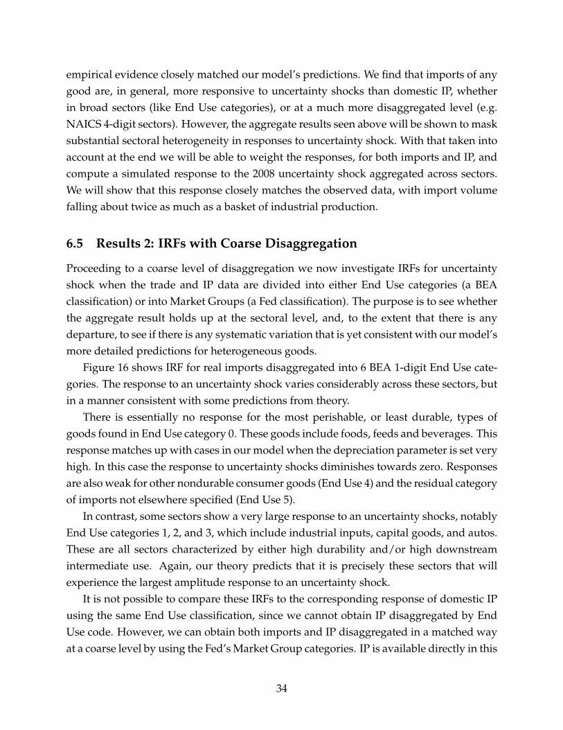
empirical evidence closely matched our model’s predictions. We find that imports of anygood are, in general, more responsive to uncertainty shocks than domestic IP, whetherin broad sectors (like End Use categories), or at a much more disaggregated level (e.g.NAICS 4-digit sectors). However, the aggregate results seen above will be shown to masksubstantial sectoral heterogeneity in responses to uncertainty shock. With that taken intoaccount at the end we will be able to weight the responses, for both imports and IP, andcompute a simulated response to the 2008 uncertainty shock aggregated across sectors.We will show that this response closely matches the observed data, with import volumefalling about twice as much as a basket of industrial production.

6.5 Results 2: IRFs with Coarse Disaggregation

Proceeding to a coarse level of disaggregation we now investigate IRFs for uncertaintyshock when the trade and IP data are divided into either End Use categories (a BEAclassification) or into Market Groups (a Fed classification). The purpose is to see whetherthe aggregate result holds up at the sectoral level, and, to the extent that there is anydeparture, to see if there is any systematic variation that is yet consistent with our model’smore detailed predictions for heterogeneous goods.

Figure 16 shows IRF for real imports disaggregated into 6 BEA 1-digit End Use cate-gories. The response to an uncertainty shock varies considerably across these sectors, butin a manner consistent with some predictions from theory.

There is essentially no response for the most perishable, or least durable, types ofgoods found in End Use category 0. These goods include foods, feeds and beverages. Thisresponse matches up with cases in our model when the depreciation parameter is set veryhigh. In this case the response to uncertainty shocks diminishes towards zero. Responsesare also weak for other nondurable consumer goods (End Use 4) and the residual categoryof imports not elsewhere specified (End Use 5).

In contrast, some sectors show a very large response to an uncertainty shocks, notablyEnd Use categories 1, 2, and 3, which include industrial inputs, capital goods, and autos.These are all sectors characterized by either high durability and/or high downstreamintermediate use. Again, our theory predicts that it is precisely these sectors that willexperience the largest amplitude response to an uncertainty shock.

It is not possible to compare these IRFs to the corresponding response of domestic IPusing the same End Use classification, since we cannot obtain IP disaggregated by EndUse code. However, we can obtain both imports and IP disaggregated in a matched wayat a coarse level by using the Fed’s Market Group categories. IP is available directly in this

34

Figure 16: Import IRFs by End Use category for Uncertainty Shocks

-.04

-.02

0

.02

0 6 12 18 24

Imports End Use 0

step0 = FOODS, FEEDS, AND BEVERAGES

-.04

-.02

0

.02

0 6 12 18 24

Imports End Use 1

step1 = INDUSTRIAL SUPPLIES AND MATERIALS

-.04

-.02

0

.02

0 6 12 18 24

Imports End Use 2

step2 = CAPITAL GOODS, EXCEPT AUTOMOTIVE

-.04

-.02

0

.02

0 6 12 18 24

Imports End Use 3

step3 = AUTOMOTIVE VEHICLES, PARTS AND ENGINES

-.04

-.02

0

.02

0 6 12 18 24

Imports End Use 4

step4 = CONSUMER GOODS (NONFOOD), EXCEPT AUTOMOTIVE

-.04

-.02

0

.02

0 6 12 18 24

Imports End Use 5

step5 = IMPORTS, N.E.S.

Source: Sample is 1989:1–2012:2. Imports by End Use 1-digit from USITC dataweb, deflated by CPI; all otherdata as in Bloom (2009), updated. Uncertainty shocks for quadvariate VARs as in Bloom (2009). Ordering isstock market, volatility, log employment, followed lastly by either log real imports or log IP. Data updatedthrough February 2012. No rescaling of shocks. 95% confidence intervals shown. See text.

format on a monthly basis and we were able to allocate imports to this classification byconstructing a concordance (with some weighting using 2002 data on weights) mappingfrom 4-digit NAICS imports to Fed Market Group.

Figure 17 shows IRF for real imports (upper panel) and IP (lower panel) disaggre-gated into Fed Market Group categories. Again, the response to an uncertainty shockvaries considerably across these sectors, and we can compare the import and IP responsesdirectly. To facilitate this, all responses are shown on the same scale.

In panel (a) the results for imports are compatible with those above based on the EndUse categories. Here, under the Fed Market Groups the largest amplitude responses toan uncertainty shock are seen for materials, business equipment and consumer durables.The responses here are between a 1 and 2 percent drop at peak. The weakest response is

35

for consumer nondurables, which shows about a 0.5 percent drop at the peak, althoughthis is barely statistically significant at the 95% level.

By contrast, in panel (b) the results for IP are very muted indeed. Confidence intervalsare tighter, so these responses do in all cases breach the 95% confidence interval withina range of steps. However, the magnitude of the response is qualitatively different fromimports. The consumer durables response is just below 1 percent at peak for IP, whereasit had been almost twice as large, near 1.5 percent for imports. Materials and businessequipment fall at peak by about 0.25 percent for IP, but fell about four times as much inthe case of imports. Consumer nondurables in IP are barely perturbed at all.

6.6 Results 3: IRFs with Finer Disaggregation

Our next set of results aims to study dynamic responses to uncertainty shocks at an evenfiner level of disaggregation, whilst still allowing for comparability between import andIP responses. For these purposes we move to the 3- or 4-digit NAICS level of classification,again sourcing the date from USITC dataweb and the Fed G.17 releases at a monthlyfrequency starting in 1989. The overlap between these two sources allows us to workwith 51 individual sectors, as seen in Figure 18. A list of NAICS codes is provided in theempirical appendix.

A similar pattern emerges here, consistent with previous results, whereby the respon-siveness in any sector is higher for real imports (CPI deflated) than for industrial produc-tion. There are some exceptions but these are generally to be found in only a few sectors.The bars in Figure 18 is ordered from top to bottom starting with largest negative realimport response measured by the average sectoral IRF over months 1–12.

Some of the sectors are also obviously quite peculiar. One is basically a nonmanufac-turing sector, and not very tradable — namely logging (NAICS 1133, which is resourceintensive and not highly traded outside imports from Canada). This does fit the generalpattern of imports being more volatile than domestic output, but this may reflect down-stream use in the heavily procyclical construction industry (we discuss downstream usein the next section). Another oddity is tobacco manufacturing (NAICS 3122), where theresponse goes heavily against the prevailing pattern, with tobacco imports rising sharplyafter an uncertainty shock, and domestic supply basically flat. Still, this response is con-sistent with clinical studies which show that the use of tobacco may rise, and the abilityof people to quit smoking may fall, in stressful periods of economic hard times.

Less unusual cases where the negative response of IP exceeds real imports are: Au-dio and video equipment manufacturing (NAICS 3343); Household and institutional fur-

36

Figure 17: Import and IP IRFs by Fed Market Group for Uncertainty Shocks

(a) Real imports

-.04

-.02

0

.02

0 10 20 30

Mkt.Grp.1: Business equip.

step

-.04

-.02

0

.02

0 10 20 30

Mkt.Grp.2: Consumer goods

step

-.04

-.02

0

.02

0 10 20 30

Mkt.Grp.3: Consumer durables

step

-.04

-.02

0

.02

0 10 20 30

Mkt.Grp.6: Materials

step

-.04

-.02

0

.02

0 10 20 30

Mkt.Grp.8: Consumer nondurables

step

(b) Industrial production

-.04

-.02

0

.02

0 10 20 30

Mkt.Grp.1: Business equip.

step

-.04

-.02

0

.02

0 10 20 30

Mkt.Grp.2: Consumer goods

step

-.04

-.02

0

.02

0 10 20 30

Mkt.Grp.3: Consumer durables

step

-.04

-.02

0

.02

0 10 20 30

Mkt.Grp.6: Materials

step

-.04

-.02

0

.02

0 10 20 30

Mkt.Grp.8: Consumer nondurables

step

Source: Sample is 1989:1–2012:2. Imports via concordance from USITC dataweb, deflated by CPI; IP fromFed G.17; all other data as in Bloom (2009), updated. Uncertainty shocks for quadvariate VARs as in Bloom(2009). Ordering is stock market, volatility, log employment, followed lastly by either log real imports orlog IP. Data updated through February 2012. No rescaling of shocks. 95% confidence intervals shown. Seetext.

37

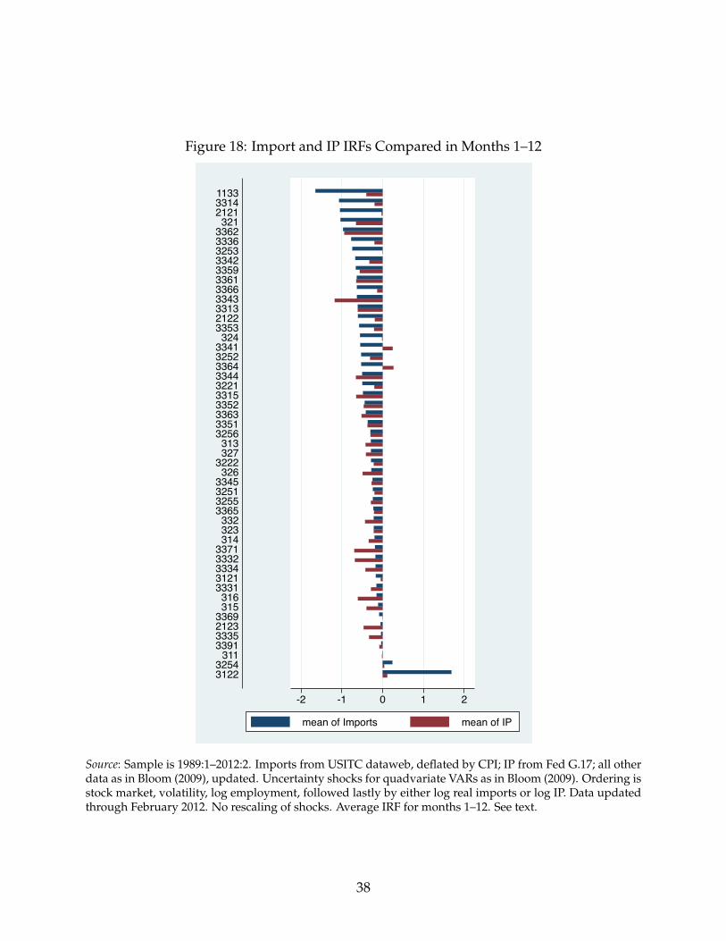
Figure 18: Import and IP IRFs Compared in Months 1–12

-2 -1 0 1 2

31223254

3113391333521233369

315316

33313121333433323371

314323332

3365325532513345

3263222

327313

3256335133633352331532213344336432523341

32433532122331333433366336133593342325333363362

321212133141133

mean of Imports mean of IP

Source: Sample is 1989:1–2012:2. Imports from USITC dataweb, deflated by CPI; IP from Fed G.17; all otherdata as in Bloom (2009), updated. Uncertainty shocks for quadvariate VARs as in Bloom (2009). Ordering isstock market, volatility, log employment, followed lastly by either log real imports or log IP. Data updatedthrough February 2012. No rescaling of shocks. Average IRF for months 1–12. See text.

38

Figure 19: Import and IP IRFs Compared in Months 1–12

1133

2121

2122

2123 3113121

3122

313314315316

321

32213222323

324

3251

32523253

3254

32553256326327

3313

3314

3315

33233313332 33343335

33363341

334233433344

334533513352

335333593361

3362

33633364

3365

3366

33693371

3391

-2-1

01

2Im

ports

IRF

(av

year

1)

-2 -1 0 1 2IP IRF (av year 1)

Source: Sample is 1989:1–2012:2. Imports from USITC dataweb, deflated by CPI; IP from Fed G.17; allother data as in Bloom (2009), updated. Uncertainty shocks for quadvariate VARs as in Bloom (2009).Ordering is stock market, volatility, log employment, followed lastly by either log real imports or log IP.Data updated through February 2012. No rescaling of shocks. Average IRF for months 1–12. See text.Notes: The correlation of the two variables is 0.2544 (with a significance level of p = .0716). However, thecorrelation falls to 0.1467 and is not statistically significant (p = .3092) when tobacco (3122) is excluded.

niture and kitchen cabinet manufacturing (3371); Industrial machinery manufacturing(3332); Ventilation, heating, air-conditioning, and commercial refrigeration equipmentmanufacturing (3334); Leather and allied product manufacturing (316); Apparel manufac-turing (315); Nonmetallic mineral mining and quarrying (2123); Metalworking machinerymanufacturing (3335). Still, out of 51 sectors, these are a minority.

But generally, and especially for the high response sectors where responses are signif-icantly different from zero, the real import bar is larger and more negative than the IP bar.The essence of this pattern is revealed in Figure 19 which presents a scatter of the averagereal import one-year IRF on the vertical axis against the average IP one-year IRF on thehorizontal axis. There is only a very weak correlation between these responses (0.25) andwhen the outlier tobacco sector is excluded the correlation essentially vanishes (it falls to0.15, but is not statistically significant).

What is more striking in the figure, however, is the general asymmetry relative to the45 degree line. Most points lie in the lower-left quadrant where both real imports and IPreact negatively to an uncertainty. In that quadrant, we do find points above the diagonal,

39

where the IP response is more negative than the real import response – but generallythese deviations from the diagonal are small. In contrast several sectors fall well belowthe diagonal by a significant margin, indicating a much sharper negative response of realimports compared to IP.

7 Inside the Black Box: Aggregate Inventory Responses

and the Role of Downstream Intermediate Use

So far our empirical analysis has taken our model seriously but looked only for vali-dation at the point where uncertainty shocks make their presence felt in the patterns ofaggregate or sectoral supply responses, whether from IP at home or imports from abroad.However, our model makes other predictions about the mechanisms whereby these un-certainty shocks feed into the supply responses, and we would like to check these inter-mediate linkages to see whether the entire story fits together at each step; that is, to getbeyond the “black box” of the impulse responses seen so far and look for further corrob-oration in other dynamics. In this section we do that by looking at two other series andtheir response to the uncertainty shocks.

7.1 Aggregate IRFs for Input Inventories

The first thing we check is aggregate input inventories of domestic (U.S.) firms. If ourargument is true, then the response of these inventories, denoted “materials and supplies"in the NIPA data from BEA (real 2005 prices, seasonally adjusted), should also show asignature of the uncertainty shock. We are careful to focus only on this component ofNIPA inventories, and exclude “work in process” and “finished goods” items as these donot correspond to quantities in our model, where the key concept is input inventories.However, one shortcoming is that the NIPA inventories data are classified by the sectorof the good produced, and are not broken down according to the sector of origin of theinput used. It is the latter we would ideally like to see, so as to match responses with, say,the NAICS disaggregated IP and import data which represent the supply of goods beingdemanded as input classified by input type. At present, we have yet to find a direct wayaround this data limitation.

Pressing on, Figure 20 shows the IRF for input inventories of materials and suppliesat the aggregate level. Sample is 1989:1–2012:12, so that the start date matches the 1989beginning year of our disaggregated data samples, and runs through 2012. The messageis clear that, despite, possible aggregation biases, the level of input inventories does show

40

Figure 20: Aggregate IRF for Input Inventories

-.02

-.01

0

.01

0 10 20 30 40

varbasic, cvolatbl, clrimpReal imports

stepGraphs by irfname, impulse variable, and response variable

Source: Sample is 1989:1–2012:12. Response is for real inventories, materials and supplies, all manufactur-ing, real 2005 prices, seasonally adjusted, from BEA NIPA. IP from Fed G.17; all other data as in Bloom(2009), updated. Uncertainty shocks for quadvariate VARs as in Bloom (2009). Ordering is stock market,volatility, log employment, followed lastly by real inventories. Data updated through December 2012. Norescaling of shocks. Average IRF for months 1–12. See text.

a negative response to uncertainty shocks, although this is small and somewhat delayed.The scale of this effect is bound to be small, however, compared to our earlier results,given that NIPA input inventories are measured as a stock whereas all of our earlier resultspertain to flows, of either IP or imports.

We also have to recognize another shortcoming here: we are looking at input on handas inventories and these may not decline as much as actual input orders themselves, be-cause the decline in stocks will be to some extent mitigated by the decline in industrialactivity itself in the using sector. [references to be added]

7.2 Disaggregated IRFs versus Downstream Intermediate Use

The second thing we look at is the relationship of the uncertainty IRFs to the intermediateinput characteristics of the goods looking at the covariation of the IRFs with a measureof downstream intermediate use (see Levchenko, Lewis and Tesar 2010). Whilst not asclean as a direct input measure, we lack that on a flow or order basis for the using sector,or even in the aggregate, as noted above, and can only use aggregate input stocks. So at

41

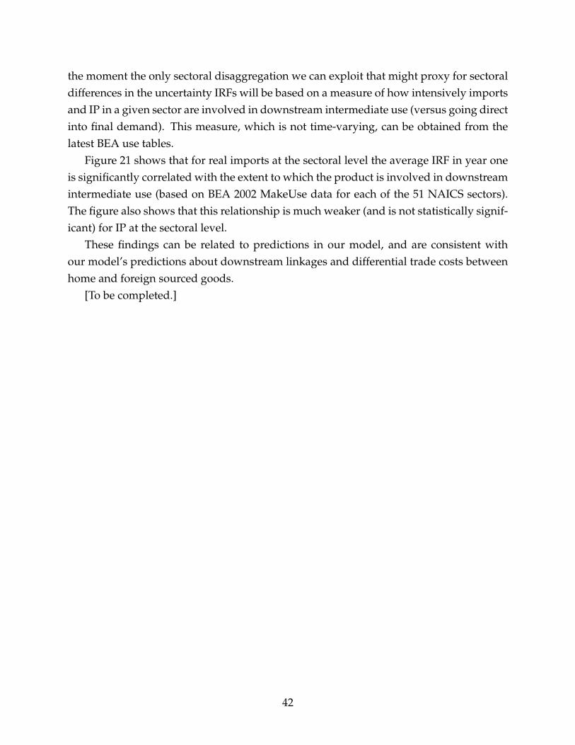
the moment the only sectoral disaggregation we can exploit that might proxy for sectoraldifferences in the uncertainty IRFs will be based on a measure of how intensively importsand IP in a given sector are involved in downstream intermediate use (versus going directinto final demand). This measure, which is not time-varying, can be obtained from thelatest BEA use tables.

Figure 21 shows that for real imports at the sectoral level the average IRF in year oneis significantly correlated with the extent to which the product is involved in downstreamintermediate use (based on BEA 2002 MakeUse data for each of the 51 NAICS sectors).The figure also shows that this relationship is much weaker (and is not statistically signif-icant) for IP at the sectoral level.

These findings can be related to predictions in our model, and are consistent withour model’s predictions about downstream linkages and differential trade costs betweenhome and foreign sourced goods.

[To be completed.]

42

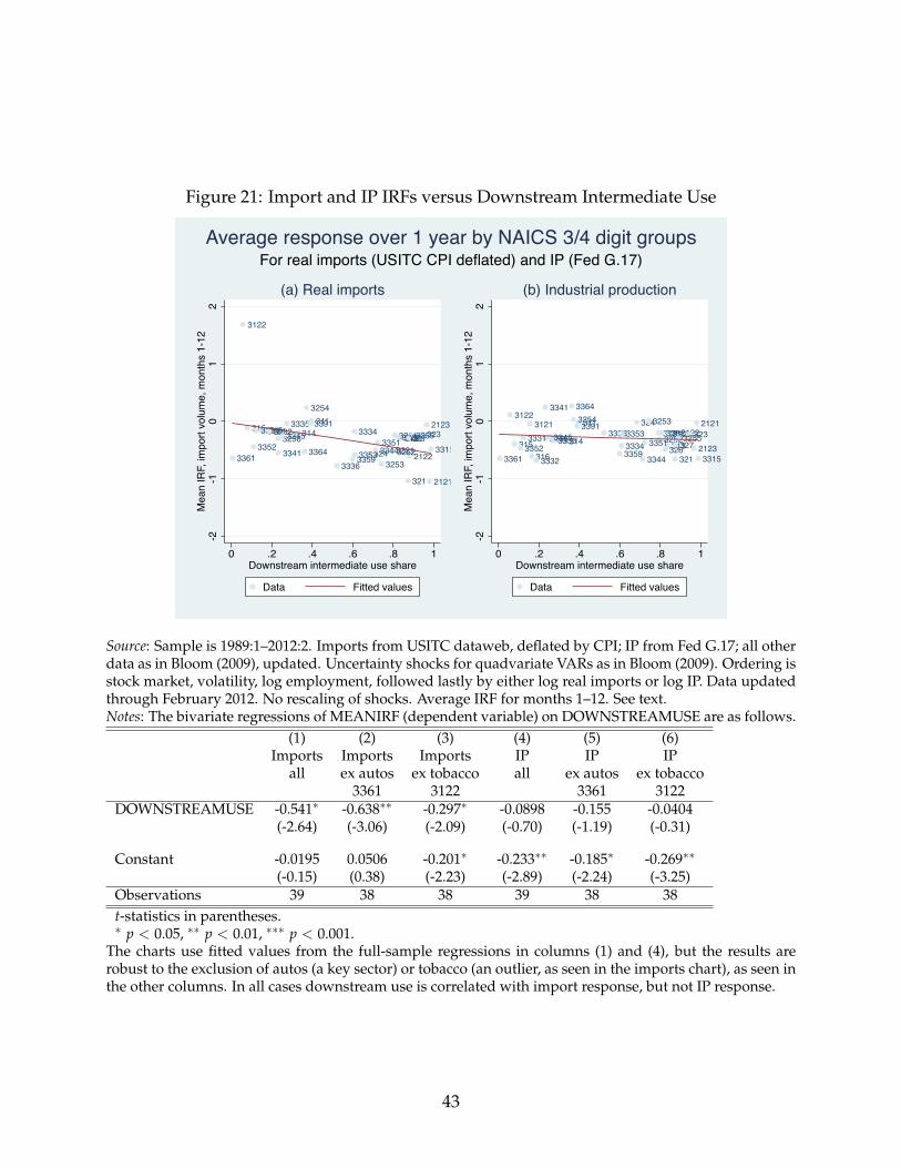
Figure 21: Import and IP IRFs versus Downstream Intermediate Use

2121

2122

21233113121

3122

313314315 316

321

32213222 323

324

3251

32523253

3254

32553256 3263273315

33313332 33343335

33363341 33443345

33513352335333593361

3364

3391

-2-1

01

2M

ean

IRF,

impo

rt vo

lum

e, m

onth

s 1-

12

0 .2 .4 .6 .8 1Downstream intermediate use share

Data Fitted values

(a) Real imports

21212122

2123

31131213122

313314315316 321

32213222 323324

32513252

32533254

32553256326327

3315

3331

333233343335

3336

3341

3344

3345 335133523353

33593361

3364

3391

-2-1

01

2M

ean

IRF,

impo

rt vo

lum

e, m

onth

s 1-

12

0 .2 .4 .6 .8 1Downstream intermediate use share

Data Fitted values

(b) Industrial production

For real imports (USITC CPI deflated) and IP (Fed G.17)Average response over 1 year by NAICS 3/4 digit groups

Source: Sample is 1989:1–2012:2. Imports from USITC dataweb, deflated by CPI; IP from Fed G.17; all otherdata as in Bloom (2009), updated. Uncertainty shocks for quadvariate VARs as in Bloom (2009). Ordering isstock market, volatility, log employment, followed lastly by either log real imports or log IP. Data updatedthrough February 2012. No rescaling of shocks. Average IRF for months 1–12. See text.Notes: The bivariate regressions of MEANIRF (dependent variable) on DOWNSTREAMUSE are as follows.

(1) (2) (3) (4) (5) (6)Imports Imports Imports IP IP IP

all ex autos ex tobacco all ex autos ex tobacco3361 3122 3361 3122

DOWNSTREAMUSE -0.541∗ -0.638∗∗ -0.297∗ -0.0898 -0.155 -0.0404(-2.64) (-3.06) (-2.09) (-0.70) (-1.19) (-0.31)

Constant -0.0195 0.0506 -0.201∗ -0.233∗∗ -0.185∗ -0.269∗∗

(-0.15) (0.38) (-2.23) (-2.89) (-2.24) (-3.25)Observations 39 38 38 39 38 38t-statistics in parentheses.∗ p < 0.05, ∗∗ p < 0.01, ∗∗∗ p < 0.001.

The charts use fitted values from the full-sample regressions in columns (1) and (4), but the results arerobust to the exclusion of autos (a key sector) or tobacco (an outlier, as seen in the imports chart), as seen inthe other columns. In all cases downstream use is correlated with import response, but not IP response.

43

8 Can the Great Trade Collapse Be Explained?

The four months following the collapse of Lehman Brothers were characterized by par-ticularly strong increases in uncertainty as measured by the volatility index (Sept.–Dec.2008). To simulate this shock we observe that the own-response of volatility to itself in theorthogonalized impulse response is about 3. We perturbed the model with four succes-sive +10-unit shocks to volatility, which, given the scaling corresponds to four +30-unitshocks to the VXO index. In actuality, the VXO rose from its pre-crisis mean of about20 to almost 90 in the last quarter of 2008, and given the decay of the shocks, this set ofimpulses matches the actual path of VXO quite well, as shown in Figure 22.

Given these shocks the actual aggregate responses to IP and real imports are shown inFigure 23. As can be seen the IRF for IP is capable of explaining a large fraction of actualobserved IP response. But it is incapable of explaining the whole real import response.Our simulations can explain about 75-80 percent of the subsequent imports collapse. Butespecially in the first quarter of 2009, additional factors must be at work that are not cap-tured by heightened uncertainty. Nonetheless, this shows that the evidence is consistentwith a large fraction of the Trade Collapse being explicable in terms of second momentuncertainty shocks, rather than the conventional first moment explanations.

[Preliminary.]

Figure 22: Actual and simulated VXO, Aggregate Model20

20

2040

40

4060

60

6080

80

80100

100

10001jan2008

01jan2008

01jan200801jan2009

01jan2009

01jan200901jan2010

01jan2010

01jan201001jan2011

01jan2011

01jan201101jan2012

01jan2012

01jan2012date

date

dateVXO, actual

VXO, actual

VXO, actualVXO, simulated

VXO, simulated

VXO, simulated

44

Figure 23: Actual and simulated Real Imports and IP, Aggregate Model-.5

-.5

-.5-.4

-.4

-.4-.3

-.3

-.3-.2

-.2

-.2-.1

-.1

-.10

0

02008m10

2008m10

2008m102009m1

2009m1

2009m12009m4

2009m4

2009m42009m7

2009m7

2009m72009m10

2009m10

2009m10month

month

monthlog Real Imports, actual

log Real Imports, actual

log Real Imports, actuallog IP, actual

log IP, actual

log IP, actuallog Real Imports, simulated

log Real Imports, simulated

log Real Imports, simulatedlog IP, simulated

log IP, simulated

log IP, simulated

9 Conclusion

Following the seminal paper by Bloom (2009), we introduce second moment uncertaintyshocks into a dynamic, open-economy model of international trade. Firms import inter-mediate inputs and due to fixed costs of ordering store them according to an optimals, S inventory policy. We show that elevated uncertainty leads firms to shift down theirs, S bands. This induces a sharp trade contraction of international trade flows followedby a swift recovery. In contrast, output remains unaffected unless conventional first mo-ment shocks are introduced. Uncertainty shocks can therefore explain why trade is morevolatile than domestic economic activity.

Our results offer an explanation for the Great Trade Collapse of 2008/09 and previ-ous trade slowdowns in a way that differs from the conventional static trade models ordynamic inventory models seen before. We argue that imports and industrial productioncan be modeled as reacting to uncertainty shocks in theory and in practice. Such secondmoment shocks are needed since the required first moment shocks are either absent on theimpulse side or insufficient on the propagation side (for plausible parameters) to explainthe events witnessed. We also show that there is substantial heterogeneity in responsesat the sectoral level, both for imports and industrial production, in a way consistent withthe model.

45

References

[1] Alessandria, G., Kaboski, J., Midrigan, V., 2010a. The Great Trade Collapse of 2008–09: An Inventory Adjustment? IMF Economic Review 58, pp. 254–294.

[2] Alessandria, G., Kaboski, J., Midrigan, V., 2010b. Inventories, Lumpy Trade, andLarge Devaluations. American Economic Review 100, pp. 2304–2339.

[3] Alessandria, G., Kaboski, J., Midrigan, V., 2011. US Trade and Inventory Dynamics.American Economic Review 101 Paper & Proceedings, pp. 303–307.

[4] Amiti, M., Weinstein, D., 2011. Exports and Financial Shocks. Quarterly Journal ofEconomics 126, pp. 1841–1877.

[5] Anderson, J., van Wincoop, E., 2003. Gravity with Gravitas: A Solution to the BorderPuzzle. American Economic Review 93, pp. 170–192.

[6] Baldwin, R. (ed.), 2009. The Great Trade Collapse: Causes, Consequences andProspects. Centre for Economic Policy Research, London.

[7] Baldwin, R., Krugman, P., 1989. Persistent Trade Effects of Large Exchange RateShocks. Quarterly Journal of Economics 104, pp. 635–654.

[8] Behrens, K., Corcos, G., Mion, G., 2013. Trade Crisis? What Trade Crisis? Review ofEconomics and Statistics, forthcoming.

[9] Bems, R., Johnson, R., Yi, K., 2011. Vertical Linkages and the Collapse of GlobalTrade. American Economic Review 101, pp. 308–312.

[10] Bems, R., Johnson, R., Yi, K., 2012. The Great Trade Collapse. NBER Working Paper18632.

[11] Bloom, N., 2009. The Impact of Uncertainty Shocks. Econometrica 77, pp. 623–685.

[12] Bloom, N., Bond, S., Van Reenen, J., 2007. Uncertainty and Investment Dynamics.Review of Economic Studies 74, pp. 391–415.

[13] Bown, C. (ed.), 2011. The Great Recession and Import Protection: The Role of Tem-porary Trade Barriers. Centre for Economic Policy Research and World Bank, Wash-ington, D.C.

46

[14] Bown, C., Crowley, M., 2013. Import Protection, Business Cycles, and ExchangeRates: Evidence from the Great Recession. Journal of International Economics 90, pp.50-64.

[15] Bricongne, J., Fontagné, L., Gaulier, G., Taglioni, D., Vicard, V., (2012). Firms and theGlobal Crisis: French Exports in the Turmoil. Journal of International Economics 87, pp.134–146.

[16] Carrière-Swallow, Y., Céspedes, L., 2013. The Impact of Uncertainty Shocks inEmerging Economies. Journal of International Economics, forthcoming.

[17] Chor, D., Manova, K., 2012. Off the Cliff and Back? Credit Conditions and Interna-tional Trade during the Global Financial Crisis. Journal of International Economics 87,pp. 117–133.

[18] Dixit, A., 1989. Entry and Exit Decisions under Uncertainty. Journal of Political Econ-omy 97, pp. 620–638.

[19] Eaton, J., Kortum, S., Neiman, B., Romalis, J., 2011. Trade and the Global Recession.NBER Working Paper 16666.

[20] Engel, C., Wang, J., 2011. International Trade in Durable Goods: UnderstandingVolatility, Cyclicality, and Elasticities. Journal of International Economics 83, pp. 37–52.

[21] Evenett, S. (ed.), 2010. Tensions Contained... For Now: The 8th GTA Report. Centrefor Economic Policy Research, London.

[22] Gopinath, G., Itskhoki, O., Neiman, B., 2012. Trade Prices and the Global Trade Col-lapse of 2008–2009. IMF Economic Review 60, pp. 303–328.

[23] Gourio, F., Siemer, M., Verdelhan, A., 2013. International Risk Cycles. Journal of Inter-national Economics 89, pp. 471-484.

[24] Grossman, S., Laroque, G., 1990. Asset Pricing and Optimal Portfolio Choice in thePresence of Illiquid Durable Consumption Goods. Econometrica 58, pp. 25–51.

[25] Guiso, L., Parigi, G., 1999. Investment and Demand Uncertainty. Quarterly Journal ofEconomics 114, pp. 185–227.

[26] Handley, K., 2012. Exporting under Trade Policy Uncertainty: Theory and Evidence.Working Paper, University of Michigan.

47

[27] Handley, K., Limão, N., 2012. Trade and Investment under Policy Uncertainty: The-ory and Firm Evidence. NBER Working Paper 17790.

[28] Hassler, J., 1996. Variations in Risk and Fluctuations in Demand: A TheoreticalModel. Journal of Economic Dynamics and Control 20, pp. 1115–1143.

[29] Imbs, J., 2010. The First Global Recession in Decades. IMF Economic Review 58, pp.327-354.

[30] Kee, H., Neagu, C., Nicita, A., 2013. Is Protectionism on the Rise? Assessing NationalTrade Policies During the Crisis of 2008. Review of Economics and Statistics 95, pp. 342-346.

[31] Leibovici, F., Waugh, M., 2012. International Trade and Intertemporal Substitution.Working Paper, New York University.

[32] Levchenko, A., Lewis, L., Tesar, L., 2010. The Collapse of International Trade duringthe 2008–2009 Crisis: In Search of the Smoking Gun. IMF Economic Review 58, pp.214–253.

[33] Limão, N., Maggi, G., 2013. Uncertainty and Trade Agreements. NBER Working Pa-per 18703.

[34] McDonald, R., Siegel, D., 1986. The Value of Waiting to Invest. Quarterly Journal ofEconomics 101, pp. 707–728.

[35] Nadiri, M., Prucha, I., 1996. Estimation of the Depreciation Rate of Physical and R&DCapital in the U.S. Total Manufacturing Sector. Economic Inquiry 34, pp. 43-56.

[36] Paravisini, D., Rappoport, V., Schnabl, P., Wolfenzon, D. 2011. Dissecting the Effect ofCredit Supply on Trade: Evidence from Matched Credit-Export Data. NBER WorkingPaper 16975.

[37] Pindyck, R., 1991. Irreversibility, Uncertainty, and Investment. Journal of EconomicLiterature 29, pp. 1110–1148.

[38] Ramey, V., 1989. Inventories as Factors of Production and Economic Fluctuations.American Economic Review 79, pp. 338-354.

[39] Scarf, H., 1959. The Optimality of (S,s) Policies in the Dynamic Inventory Problem. In:Arrow, K., Karlin, S., Suppes, P. (eds.), Mathematical Methods in the Social Sciences,Stanford University Press, pp. 196–202.

48

[40] Taglioni, D., Zavacka, V., 2012. Innocent Bystanders: How Foreign UncertaintyShocks Harm Exporters. Working Paper, European Bank for Reconstruction and De-velopment.

[41] Yilmazkuday, H., 2012. The Great Trade Collapse: A Horse Race of Competing Sto-ries. Working Paper, Florida International University.

49

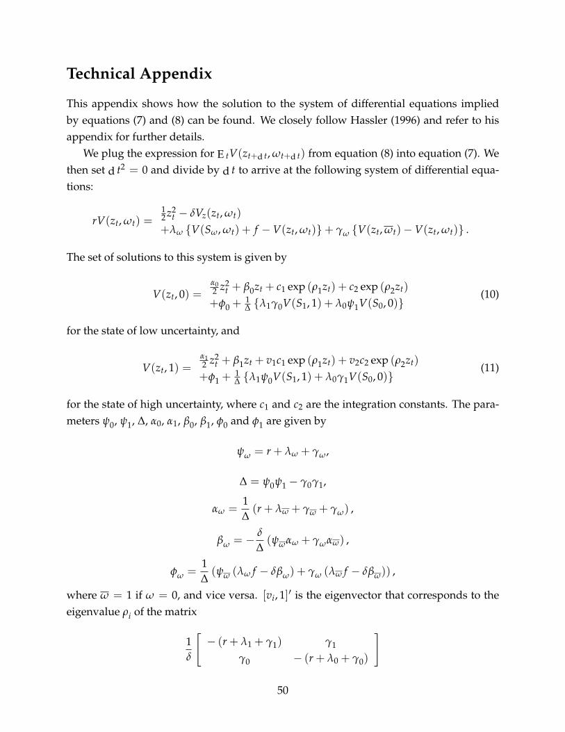
Technical Appendix

This appendix shows how the solution to the system of differential equations impliedby equations (7) and (8) can be found. We closely follow Hassler (1996) and refer to hisappendix for further details.

We plug the expression for E tV(zt+d t, ωt+d t) from equation (8) into equation (7). Wethen set d t2 = 0 and divide by d t to arrive at the following system of differential equa-tions:

rV(zt, ωt) =12 z2

t − δVz(zt, ωt)

+λω {V(Sω, ωt) + f −V(zt, ωt)}+ γω {V(zt, ωt)−V(zt, ωt)} .

The set of solutions to this system is given by

V(zt, 0) =α02 z2

t + β0zt + c1 exp (ρ1zt) + c2 exp (ρ2zt)

+φ0 +1∆ {λ1γ0V(S1, 1) + λ0ψ1V(S0, 0)}

(10)

for the state of low uncertainty, and

V(zt, 1) =α12 z2

t + β1zt + v1c1 exp (ρ1zt) + v2c2 exp (ρ2zt)

+φ1 +1∆ {λ1ψ0V(S1, 1) + λ0γ1V(S0, 0)}

(11)

for the state of high uncertainty, where c1 and c2 are the integration constants. The para-meters ψ0, ψ1, ∆, α0, α1, β0, β1, φ0 and φ1 are given by

ψω = r+ λω + γω,

∆ = ψ0ψ1 − γ0γ1,

αω =1∆(r+ λω + γω + γω) ,

βω = −δ

∆(ψωαω + γωαω) ,

φω =1∆(ψω (λω f − δβω) + γω (λω f − δβω)) ,

where ω = 1 if ω = 0, and vice versa. [vi, 1]′ is the eigenvector that corresponds to theeigenvalue ρi of the matrix

1δ

[− (r+ λ1 + γ1) γ1

γ0 − (r+ λ0 + γ0)

]

50

for i = 1, 2. Expressions for V(S0, 0) and V(S1, 1) can be obtained by setting V(zt, 0) =V(S0, 0) and V(zt, 0) = V(S1, 1) in equations (10) and (11), respectively, and then solvingthe two resulting equations.

Six key equations describe the solution. They are two value-matching conditionspositing for each state of uncertainty that the value of the cost function at the return pointmust be equal to the value at the lower trigger point less the fixed ordering costs f :

V(S0, 0) = V(s0, 0)− f ,

V(S1, 1) = V(s1, 1)− f .

The remaining four equations are smooth-pasting conditions:

Vz(S0, 0) = 0,

Vz(s0, 0) = 0,

Vz(S1, 1) = 0,

Vz(s1, 1) = 0.

These six conditions determine the six key parameters: the return points S0 and S1, thelower trigger points s0 and s1 as well as the two integration constants c1 and c2. Numericalmethods have to be used to find them.

51

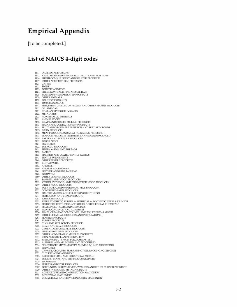
Empirical Appendix

[To be completed.]

List of NAICS 4-digit codes

1111 OILSEEDS AND GRAINS1112 VEGETABLES AND MELONS 1113 FRUITS AND TREE NUTS1114 MUSHROOMS, NURSERY AND RELATED PRODUCTS1119 OTHER AGRICULTURAL PRODUCTS1121 CATTLE1122 SWINE1123 POULTRY AND EGGS1124 SHEEP, GOATS AND FINE ANIMAL HAIR1125 FARMED FISH AND RELATED PRODUCTS1129 OTHER ANIMALS1132 FORESTRY PRODUCTS1133 TIMBER AND LOGS1141 FISH, FRESH, CHILLED OR FROZEN AND OTHER MARINE PRODUCTS2111 OIL AND GAS2121 COAL AND PETROLEUM GASES2122 METAL ORES2123 NONMETALLIC MINERALS3111 ANIMAL FOODS3112 GRAIN AND OILSEED MILLING PRODUCTS3113 SUGAR AND CONFECTIONERY PRODUCTS3114 FRUIT AND VEGETABLE PRESERVES AND SPECIALTY FOODS3115 DAIRY PRODUCTS3116 MEAT PRODUCTS AND MEAT PACKAGING PRODUCTS3117 SEAFOOD PRODUCTS PREPARED, CANNED AND PACKAGED3118 BAKERY AND TORTILLA PRODUCTS3119 FOODS, NESOI3121 BEVERAGES3122 TOBACCO PRODUCTS3131 FIBERS, YARNS, AND THREADS3132 FABRICS3133 FINISHED AND COATED TEXTILE FABRICS3141 TEXTILE FURNISHINGS3149 OTHER TEXTILE PRODUCTS3151 KNIT APPAREL3152 APPAREL3159 APPAREL ACCESSORIES3161 LEATHER AND HIDE TANNING3162 FOOTWEAR3169 OTHER LEATHER PRODUCTS3211 SAWMILL AND WOOD PRODUCTS3212 VENEER, PLYWOOD, AND ENGINEERED WOOD PRODUCTS3219 OTHER WOOD PRODUCTS3221 PULP, PAPER, AND PAPERBOARD MILL PRODUCTS3222 CONVERTED PAPER PRODUCTS3231 PRINTED MATTER AND RELATED PRODUCT, NESOI3241 PETROLEUM AND COAL PRODUCTS3251 BASIC CHEMICALS3252 RESIN, SYNTHETIC RUBBER, & ARTIFICIAL & SYNTHETIC FIBERS & FILIMENT3253 PESTICIDES, FERTILIZERS AND OTHER AGRICULTURAL CHEMICALS3254 PHARMACEUTICALS AND MEDICINES3255 PAINTS, COATINGS, AND ADHESIVES3256 SOAPS, CLEANING COMPOUNDS, AND TOILET PREPARATIONS3259 OTHER CHEMICAL PRODUCTS AND PREPARATIONS3261 PLASTICS PRODUCTS3262 RUBBER PRODUCTS3271 CLAY AND REFRACTORY PRODUCTS3272 GLASS AND GLASS PRODUCTS3273 CEMENT AND CONCRETE PRODUCTS3274 LIME AND GYPSUM PRODUCTS3279 OTHER NONMETALLIC MINERAL PRODUCTS3311 IRON AND STEEL AND FERROALLOY3312 STEEL PRODUCTS FROM PURCHASED STEEL3313 ALUMINA AND ALUMINUM AND PROCESSING3314 NONFERROUS METAL (EXCEPT ALUMINUM) AND PROCESSING3315 FOUNDRIES3321 CROWNS, CLOSURES, SEALS AND OTHER PACKING ACCESSORIES3322 CUTLERY AND HANDTOOLS3323 ARCHITECTURAL AND STRUCTURAL METALS3324 BOILERS, TANKS, AND SHIPPING CONTAINERS3325 HARDWARE3326 SPRINGS AND WIRE PRODUCTS3327 BOLTS, NUTS, SCREWS, RIVETS, WASHERS AND OTHER TURNED PRODUCTS3329 OTHER FABRICATED METAL PRODUCTS3331 AGRICULTURE AND CONSTRUCTION MACHINERY3332 INDUSTRIAL MACHINERY3333 COMMERCIAL AND SERVICE INDUSTRY MACHINERY

52

3334 VENTILATION, HEATING, AIR-CONDITIONING, AND COMMERCIAL REFRIGERATION EQUIPMENT3335 METALWORKING MACHINERY3336 ENGINES, TURBINES, AND POWER TRANSMISSION EQUIPMENT3339 OTHER GENERAL PURPOSE MACHINERY3341 COMPUTER EQUIPMENT3342 COMMUNICATIONS EQUIPMENT3343 AUDIO AND VIDEO EQUIPMENT3344 SEMICONDUCTORS AND OTHER ELECTRONIC COMPONENTS3345 NAVIGATIONAL, MEASURING, ELECTROMEDICAL, AND CONTROL INSTRUMENTS3346 MAGNETIC AND OPTICAL MEDIA3351 ELECTRIC LIGHTING EQUIPMENT3352 HOUSEHOLD APPLIANCES AND MISCELLANEOUS MACHINES, NESOI3353 ELECTRICAL EQUIPMENT3359 ELECTRICAL EQUIPMENT AND COMPONENTS, NESOI3361 MOTOR VEHICLES3362 MOTOR VEHICLE BODIES AND TRAILERS3363 MOTOR VEHICLE PARTS3364 AEROSPACE PRODUCTS AND PARTS3365 RAILROAD ROLLING STOCK3366 SHIPS AND BOATS3369 TRANSPORTATION EQUIPMENT, NESOI3371 HOUSEHOLD AND INSTITUTIONAL FURNITURE AND KITCHEN CABINETS3372 OFFICE FURNITURE (INCLUDING FIXTURES)3379 FURNITURE RELATED PRODUCTS, NESOI3391 MEDICAL EQUIPMENT AND SUPPLIES3399 MISCELLANEOUS MANUFACTURED COMMODITIES5111 NEWSPAPERS, BOOKS & OTHER PUBLISHED MATTER, NESOI5112 SOFTWARE, NESOI5122 PUBLISHED PRINTED MUSIC AND MUSIC MANUSCRIPTS9100 WASTE AND SCRAP9200 USED OR SECOND-HAND MERCHANDISE9800 GOODS RETURNED TO CANADA (EXPORTS ONLY); U.S. GOODS RETURNED AND REIMPORTED ITEMS (IMPORTS ONLY)9900 SPECIAL CLASSIFICATION PROVISIONS, NESOI

53