trade, firms, and wages: theory and evidencedrd28/wages_amiti_and_davis.pdf · the trade...

“rdr016” — 2012/1/31 — 19:28 — page 1 — #1

Review of Economic Studies (2011)79, 1–36 doi: 10.1093/restud/rdr016 The Author 2011. Published by Oxford University Press on behalf of The Review of Economic Studies Limited.Advance access publication 22 August 2011

Trade, Firms, and Wages:Theory and Evidence

MARY AMITIFederal Reserve Bank of New York and CEPR

andDONALD R. DAVIS

ColumbiaUniversity and NBER

First version received April2009; final version accepted March2011 (Eds.)

How does trade liberalization affect wages? This is the first paper to consider in theory and data howthe impact of final and intermediate input tariff cuts on workers’ wages varies with the global engagementof their firm. Our model predicts that a fall in output tariffs lowers wages at import-competing firms butboosts wages at exporting firms. Similarly, a fall in input tariffs raises wages at import-using firms relativeto those at firms that only source inputs locally. Using highly detailed Indonesian manufacturing censusdata for the period 1991–2000, we find considerable support for the model’s predictions.

Key words: Input tariffs, Output tariffs, Firm heterogeneity, Trade liberalization

JEL Codes: F10, F12, F13, F14

1. INTRODUCTION

How does trade liberalization affect wages? This is one of the most important questions in in-ternational economics, one that has generated a vast theoretical and empirical literature.1 Yet nocontribution to this literature has simultaneously addressed the two most salient facts to emergein the last decade about international production. The first fact is the role of firm-level hetero-geneity in export and import behaviour. As emphasized inBernardet al. (2007), exporting andimporting are concentrated in a small number of firms that are larger, more productive, and payhigher wages. The second fact is the large and growing importance of trade in intermediates,as documented byYi (2003). A distinct role for intermediates is of considerable importance, aswell, because of the contrasting protective and anti-protective effects of final and intermediatetariffs, respectively.

The contribution of this paper is to examine, theoretically and empirically, the impact of tradeliberalization on wages while taking explicit account of both of these facts. We develop a generalequilibrium model that features firm heterogeneity, trade in final and intermediate products, andfirm-specific wages. In doing so, it builds on the work on heterogeneous firms ofMelitz (2003)as amended to allow trade in intermediate goods byKasahara and Lapham(2007). Both of these

1. For recent contributions, see the papers inHarrison(2007) and the surveys byGoldberg and Pavcnik(2007)andFeenstra and Hanson(2003).

1

at Colum

bia University L

ibraries on March 12, 2012

http://restud.oxfordjournals.org/D

ownloaded from

http://restud.oxfordjournals.org/

“rdr016” — 2012/1/31 — 19:28 — page 2 — #2

2 REVIEW OF ECONOMIC STUDIES

models maintain the assumption of homogeneous labour and a perfect labour market, so thatthe wages paid by a firm are disconnected from that firm’s performance. We continue to focuson homogeneous labour but introduce a variant of fair wages most closely related to that ofGrossman and Helpman(2007).

The key theoretical result is that the wage consequence of a particular tariff change dependson the mode of globalization of the firm at which a worker is employed. A decline in outputtariffs reduces wages of workers at firms that sell only in the domestic market, but raises wagesof workers at firms that export. A decline in input tariffs raises the wages of workers at firmsusing imported inputs, but reduces wages at firms that do not import inputs. And there is asynergy in these effects so that exporting or importing magnifies the effect of the other.

We test our model’s hypotheses with a rich data set covering the Indonesian trade liberaliza-tion of 1991–2000. The trade liberalization provides us with over 500 price changes per period,covering both input and output tariffs. A distinctive feature of the Indonesian data set is theavailability of firm-level data on individual inputs, making it possible to construct highly dis-aggregated input tariffs. This, in turn, enables us to disentangle the effects of output and inputtariffs. The data cover a period with a very substantial liberalization of both types of tariffs, withimportant variation across and within industries. From 1991 to 2000, average output tariffs fellfrom 21% to 8%, while average input tariffs fell from 14% to 6%. Further, the data include infor-mation on firm-level importing and exporting behaviour, allowing us to identify the differentialeffects of trade liberalization on exporters, importers, and domestically oriented firms.

The results of our study are striking. First, heterogeneity matters. Not only are firms affectedin a heterogeneous way by trade liberalization, but so are the wages of their workers. Second,modes of globalization matter. Liberalization in final and intermediate goods trade have distinctimpacts on the fate of workers according to the modes of globalization of the firms at which theywork. A 10% point fall in output tariffs decreases wages by 3% in firms oriented exclusivelytoward the domestic economy. But the same fall in the output tariffincreaseswages by up to3% in firms that export. A 10% point fall in input tariffs has an insignificant effect on firms thatdo not import butincreaseswages by up to 12% in firms that do import. In short, liberalizationalong each dimension raises wages for workers at firms that are most globalized and lowerswages at firms oriented to the domestic economy or which are marginal globalizers. Ours isthe first paper to show an empirical link between input tariffs and wages, and the first to showdifferential effects from reducing output tariffs on exporters and non-exporters.

Our results both parallel, and diverge from, findings in previous studies. The literature hasfound inconsistent results of the effect of output tariff cuts on wages. For example, both theindustry-level study on Colombia byGoldberg and Pavcnik(2005) and the firm-level study onMexico byRevenga(1997) associate a cut in output tariffs with a decline in industry and firmwages, respectively. However, the industry-level study on Brazil byPavcniket al.(2004) and thefirm-level study of North American Free Trade Agreement byTrefler (2004) find insignificantor near zero effects of a decline in output tariffs on wages. None of the prior studies has foundthat cuts in output tariffsraisethe wages of workers at some firms. Our approach, which allowsthe effect of output tariffs on firm wages to depend on the firm’s export orientation, may explainthe prior mixed results due to the pooling of groups of firms with disparate responses.

Differential firm-level wage responses between exporters and non-exporters arise inVerhoogen(2008). However, the experiment he considers is not a trade liberalization but ratheran exchange rate depreciation. Implicitly, this is a movement in a single price. But the samedevaluation that makes exporting more attractive also makes importing intermediates less attrac-tive, and one can hope at best to ascertain the net of the two effects. The first study to placeimported intermediates at the heart of a discussion of wage evolution isFeenstra and Hanson(1999). But their study only considers economy-wide wage changes and their empirical exercise

at Colum

bia University L



ownloaded from


“rdr016” — 2012/1/31 — 19:28 — page 3 — #3

AMITI & DAVIS TRADE, FIRMS, AND WAGES 3

includes no explicit measures of changes in the costs of importing intermediates (tariff reduc-tions or otherwise). Indeed, no prior study has used explicit measures of liberalization in inter-mediate tariffs to estimate wage effects.

Our empirical results directly address the effect of tariff liberalization on firm-level wages,but the results have broader implications. The theoretical results encompass any element ofglobalization in which there is a change in the relative marginal cost of serving final goodsmarkets or sourcing inputs from foreign vs. domestic markets. This includes changes in transportcosts, regulation, or other barriers that affect these relative marginal costs. From this perspective,the advantage of our experiment in understanding the broader process of globalization is thattariff liberalization allows these changes in relative marginal costs to be measured precisely andso give us greater ability to identify the consequences for firm-level wages.

2. THEORY

Our theory draws on three key elements. The first is heterogeneous firms, as inMelitz (2003).The second is costly trade in intermediates, as inKasahara and Lapham(2007). The third isimperfect factor markets that feature some form of rent sharing between firm and workers, as,e.g., in Helpman, Itskhoki and Redding(2010).2

2.1. Consumptionof final goods

Final demand is directly fromDixit and Stiglitz (1977). Consumers allocate expendituresEacross a continuum of available final good varieties to

Min E =∫

p(ν)q(ν)dν s.t.

[∫q(ν)

σ−1σ dν

] σσ−1

= U . (1)

Here,σ > 1 is the elasticity of substitution between final goods varieties. These deliver de-mand curves for final productν of the formq(ν) =

[ p(ν)P

]−σQ andrevenue of the formr (ν) =

R[ p(ν)

P

]1−σ , whereQ ≡ U , andP is an aggregate price index given byP =[ ∫

ν∈Vp(ν)1−σ dν

] 11−σ

with PQ = R.

2.2. The fair-wage constraint and the labour market

Our data exercise focuses on the evolution of firm specific wages, and so our theory must providefor these. We do this with two elements. The first is firm heterogeneity, both in productivity andin firm-specific costs of penetrating international markets. The second is to tie firm wages to firmperformance. We introduce this via a fair-wage constraint.

Our model will feature firms, some of whose operating profits are zero and others for whichthese are positive. Firms earning zero profits are either in a competitive intermediates sector ormarginal firms in an imperfectly competitive final goods sector in which all other firms havepositive operating profits.

Workers have fair-wage demands. All workers at zero-profit firms earn the same wage,whether in the intermediate or final goods sectors. We take this wage as our numéraire. Let-ting the wage on offer at any other firmν be given asWν . We assume that other firms pay a wage

2. Imperfect factor markets that feature firm-worker rent sharing is key. The precise form this takes is not essentialto our story and, at this stage and with this data, we do not aim to distinguish them. The literature has considered searchmodels withex postbargaining, as inFelbermayret al. (2011) orHelpman, Itskhoki and Redding(2010); efficiencywage models, as inDavis and Harrigan(2011); and fair-wage models, as inEgger and Kreickemeier(2009) and thepresent paper.

at Colum

bia University L



ownloaded from


“rdr016” — 2012/1/31 — 19:28 — page 4 — #4


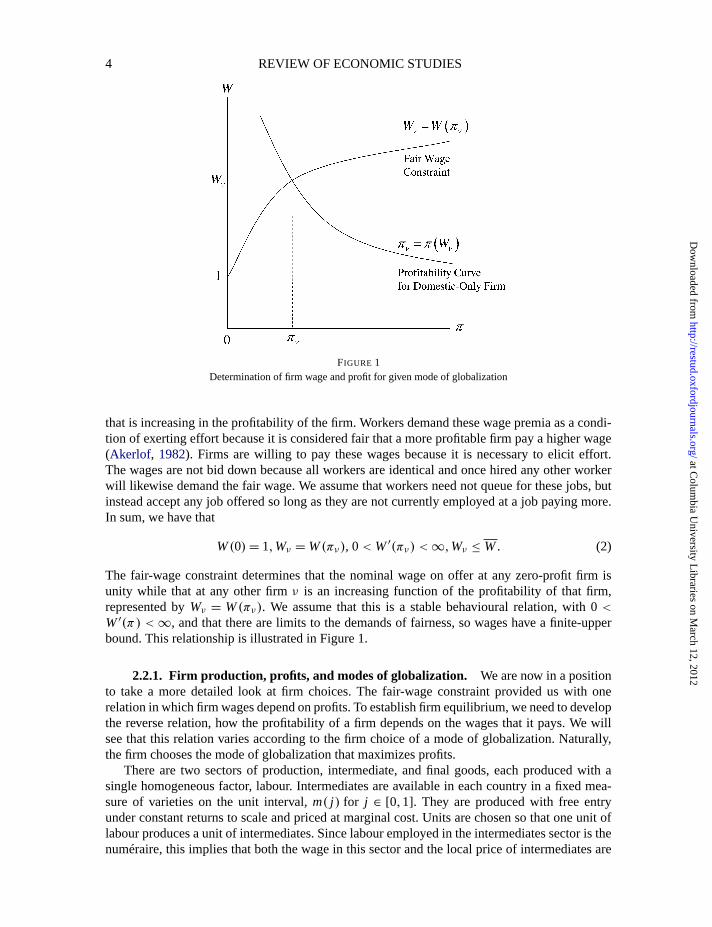
FIGURE 1Determination of firm wage and profit for given mode of globalization

that is increasing in the profitability of the firm. Workers demand these wage premia as a condi-tion of exerting effort because it is considered fair that a more profitable firm pay a higher wage(Akerlof, 1982). Firms are willing to pay these wages because it is necessary to elicit effort.The wages are not bid down because all workers are identical and once hired any other workerwill likewise demand the fair wage. We assume that workers need not queue for these jobs, butinstead accept any job offered so long as they are not currently employed at a job paying more.In sum, we have that

W(0) = 1,Wν = W(πν), 0< W′(πν) < ∞,Wν ≤ W. (2)

The fair-wage constraint determines that the nominal wage on offer at any zero-profit firm isunity while that at any other firmν is an increasing function of the profitability of that firm,represented byWν = W(πν). We assume that this is a stable behavioural relation, with 0<W′(π) < ∞, and that there are limits to the demands of fairness, so wages have a finite-upperbound. This relationship is illustrated in Figure 1.

2.2.1. Firm production, profits, and modes of globalization. We are now in a positionto take a more detailed look at firm choices. The fair-wage constraint provided us with onerelation in which firm wages depend on profits. To establish firm equilibrium, we need to developthe reverse relation, how the profitability of a firm depends on the wages that it pays. We willsee that this relation varies according to the firm choice of a mode of globalization. Naturally,the firm chooses the mode of globalization that maximizes profits.

There are two sectors of production, intermediate, and final goods, each produced with asingle homogeneous factor, labour. Intermediates are available in each country in a fixed mea-sure of varieties on the unit interval,m( j ) for j ∈ [0,1]. They are produced with free entryunder constant returns to scale and priced at marginal cost. Units are chosen so that one unit oflabour produces a unit of intermediates. Since labour employed in the intermediates sector is thenuméraire, this implies that both the wage in this sector and the local price of intermediates are

at Colum

bia University L



ownloaded from


“rdr016” — 2012/1/31 — 19:28 — page 5 — #5


unity. At this price, intermediate suppliers stand ready to meet any demand arising in the finalgoods sector.3

In the final goods sector, the sequence of decision problems is based onMelitz (2003). Froman unbounded mass of potential firms, a massMe paysa fixed costfe in units of labour. Havingpaid this fixed cost, the firm receives a random draw that reveals a triplet of informationλν =(φν, tMν, tXν) thatis distributed with the joint probability density functiong(λν). The respectiveelements are the firm’s productivity in marginal cost activitiesφν aswell as the idiosyncraticcomponents of marginal trade costs in importstMν andexportstXν .

We add these additional dimensions of firm heterogeneity to match cross-sectional featuresof the data. If, as in Melitz, the marginal physical productivity parameterϕ were the only di-mension of firm heterogeneity, then we could have at most three of the four types of firms active(either all exporters would also import or all importers would also export rather than allowingeach separately). Introduction of one additional dimension of firm heterogeneity would sufficeto solve this issue. The reason for adding two additional dimensions of heterogeneity (exportand import costs) is because, otherwise, all firms that export would export the same share oftheir output or all firms that import would import the same share of their inputs. The cross-sectional data instead strongly show large variation in export and import shares, hence motivateour assumptions. While we characterizetXν andtMνastrade costs, they can also be looked on asfirm-specific marginal efficiencies, respectively, of penetrating foreign markets or using foreigninputs. All experiments considered in this paper consist of varying only common components oftrade costs,τX andτM .

For future reference, we also introduce the marginal probability densityg8(φ) ≡∫

tM

∫tX

g(λ)

dtXdtM andthe associated cumulative densityG8(φ) ≡∫ φ

0 g8(u)du. After learning their char-acteristics, some firms exit without producing, and the remaining mass of firmsM will chooselabour and intermediate inputs as well as final outputs destined for each market to maximizeprofits. There is a constant hazard rateδ of firm death. Steady state requires that new entrymatches firm exits.

At any point in time, the individual final goods producer maximizes profits, taking the de-mand curve as given. We assume that all fixed cost activities pay a wage in constant proportionto that available in the competitive intermediates sector, which we set at unity for convenience.4

However, we will focus on firm-specific wagesWν in variable cost activities that arise in equi-librium, as developed below. In order to produce in any period, a final goods firm is requiredto employ f units of labour in fixed costs. With the fixed costs incurred, production is Cobb–Douglas in labour and intermediates.

We show in the electronic appendix that firms behave as if marginal costs are constant at theirequilibrium level. Thus, we must derive a functional relation between profits at the firm and thewages paid there for each mode of globalization. For given macro variables, this will allow thefirm to choose the mode of globalization that maximizes profits, determining also wages and allother firm variables.

Profits for a firm in the isoelastic setting with constant marginal costs are generically givenas

πν = Max[0,

rν

σ− Fν

]. (3)

3. We allow for love of variety in intermediates but fix the measure of varieties per market exogenously. Thisallows us to introduce the desired cost-saving aspect of intermediate trade without the complications, including multipleequilibria, familiar from economic geography models such asVenables(1996).

4. Our assumption that fixed costs are invariant here to changes in firm wages for variable cost labour is forsimplicity and parallels the assumption inHelpman, Itskhoki and Redding(2010), where firm-fixed costs are paid in acompetitive outside good.

at Colum

bia University L



ownloaded from


“rdr016” — 2012/1/31 — 19:28 — page 6 — #6


The fixed costFν for a firm is a function of the mode of globalization. Letn be the numberof foreign markets,fX be the fixed cost of penetrating an export market, andfM be the fixedcost of importing intermediates from each foreign market, then

Fν =

f if domestic only,

f +n fM if import intermediates,

f +n fX if export final goods,

f +n( fX + fM ) if export final goods and import intermediates.

(4)

In each of then + 1countries, a unit measure of intermediates is produced with labour onlyunder free entry and constant returns to scale. From above, the price of any domestic interme-diate is unity, as is the free on board price of exported intermediates. The common landed cost,insurance and freight price for imported intermediates isτM > 1, but we assume there is alsoa firm-specific iceberg component,tMν ∈ [1, tM ], that reflects a firm’s own capability in usingimported intermediates. Hence, the total effective price to a firmν is τMν = τMtMν > 1. Lib-eralization is assumed to affect only the common marginal import cost termτM . A firm withlower-idiosyncratic intermediate trade costs can more easily cover the common fixed importcost, so it will begin to import at a lower level of idiosyncratic output productivity. Because low-idiosyncratic import costs reduce the relative price of imported inputs, when such a firm importsit will also use a higher share of imported (relative to locally produced) intermediates, havehigher profits and higher wages,ceteris paribus, than a firm with higher-idiosyncratic importcosts.

Final good firms’ choices about importing intermediates will affect their costs. Marginalcostscν areCobb–Douglas in the input prices:

cν =1

φν

(Wν

α

)α( PMν

1−α

)1−α

=κWα

ν P1−αMν

φν, whereκ ≡ α−α(1−α)−(1−α). (5)

Costs feature two endogenous variables from the firm’s perspective. The first is the wage. It mustbe kept in mind that firm costs, revenues, and profits in this section are determinedconditionalon the firm wage, which is itself determined only at the end of this section. The second is theprice of the composite intermediate, which depends on whether intermediates are imported ornot due to love of variety in available intermediates. A firm that imports has, in addition to a unitinterval of local intermediates, access ton additional unit intervals of intermediates. Letγ > 1be the elasticity of substitution between any two varieties of intermediates. Then the price ofintermediatesPMν varies according to input behaviour. A firm that uses domestic inputs only

hasPMν = 1, while a firm that imports intermediates hasPMν = [1+nτ1−γMν ]

11−γ < 1.5

Hence,marginal costs depend on the choice of globalization, which affectsPMν and theequilibrium firm wageWν (determinedbelow). For a firm that does not import intermediates,marginal cost iscν = κWα

νφν

andfor a firm that does import intermediates, there is a lower marginal

cost at any given wage ofcν = κWαν

φν

(1+nτ

1−γMν

) 1−α1−γ . Given isoelastic demand and monopolistic

competition, as we saw earlier, the domestic price of a final good variety is the standard mark-upon marginal costs,pνd = σ

σ−1cν .6

5. Here we abstract from the issue of whether increased imports are due to an intensive or extensive margin, sincein both cases a tariff reduction reduces costs, raising profits and wages. Evidence on these margins may be found,interalia, in Goldberget al. (2009),Klenow and Rodriguez-Clare(1997) andArkolakiset al. (2008).

6. In an electronic appendix, we show that constant markup pricing remains optimal for the firm in spite of itsknowledge that its choices affect the wage. Intuitively, since the wage dependspositivelyon profitability, the firm has noincentive to manipulate the wage, so treats it as parametric at the equilibrium level.

at Colum

bia University L



ownloaded from


“rdr016” — 2012/1/31 — 19:28 — page 7 — #7


Revenue in the domestic market depends on the price there, as inrνd = RPσ−1p1−σνd . Since

importing intermediates affects cost, and so price, it also affects revenues. For a firm that doesnot import intermediates, revenues are given asrνd = RPσ−1

( κWαν

ρφν

)1−σ , while they are the

higherrνd = 0Mν RPσ−1( κWα

νρφν

)1−σ at a given wage for a firm that does import intermediates.

Here,0Mν ≡(1+nτ

1−γMν

) (1−α)(1−σ)1−γ > 1 is an “import globalization” factor, reflecting the reduced

marginal costs due to the use of imported intermediates, which lowers prices and raises revenues.The markup is1

ρ , whereσ = 11−ρ .

Total revenuesrν dependnot only on the degree of penetration of any one market but alsoon the effective number of markets served and the firm’s efficiency in serving those markets. Weassume that there are idiosyncratic iceberg costs for a firm to serve a foreign market, given byτXν . These can be decomposed into a common export costτX > 1 and an idiosyncratic compo-nenttXν ∈ [1, tXν ], whereτXν = τXtXν . Revenues in a foreign market are reduced proportionallyto those in the domestic market, reflecting the higher price faced by consumers in that marketdue to iceberg costsτXν on final goods exports. All else equal, a firm with idiosyncraticallylow-export costs will enter exporting at a lower level of productivity than other firms and willexport a higher share of its total output.

Lettingrνd bethe revenues of a firm that serves the domestic market only, a firm that exportswill have revenues0Xνrνd. Here,0Xν ≡ (1+nτ1−σ

Xν ) > 1 is an “export globalization” factor,reflecting the fact that in addition to the domestic market, exporting gives access ton additionalmarkets, each of which isτ1−σ

Xν < 1 times the size of the domestic market.This gives us the complete set of dimensions of globalization, depending on whether interme-

diates are imported or final goods exported. Note that so long as profits are non-negative, theseare related to revenues byπν = rν

σ − Fν . Let variable profits for a firm that is purely domestic be

πνdVar =( RPσ−1

σ

)( κWαν

ρφν

)1−σ . Then the profits, conditional on wages, are

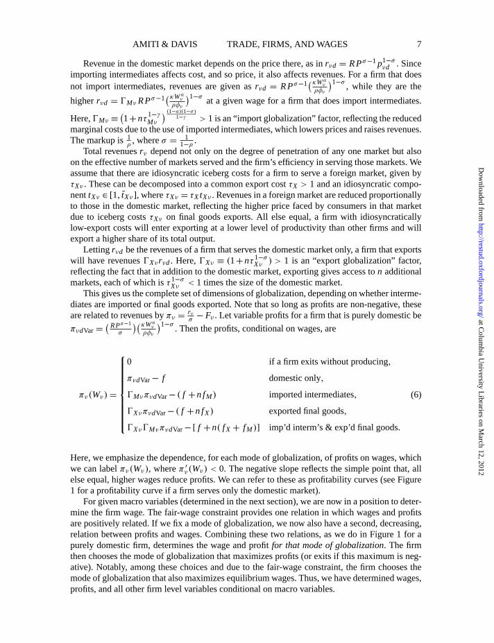
πν(Wν) =

0 if a firm exits without producing,

πνdVar− f domesticonly,

0MνπνdVar− ( f +nfM ) importedintermediates,

0XνπνdVar− ( f +nfX) exported final goods,

0Xν0MνπνdVar− [ f +n( fX + fM )] imp’d interm’s & exp’d final goods.

(6)

Here, we emphasize the dependence, for each mode of globalization, of profits on wages, whichwe can labelπν(Wν), whereπ ′

ν(Wν) < 0. The negative slope reflects the simple point that, allelse equal, higher wages reduce profits. We can refer to these as profitability curves (see Figure1 for a profitability curve if a firm serves only the domestic market).

For given macro variables (determined in the next section), we are now in a position to deter-mine the firm wage. The fair-wage constraint provides one relation in which wages and profitsare positively related. If we fix a mode of globalization, we now also have a second, decreasing,relation between profits and wages. Combining these two relations, as we do in Figure 1 for apurely domestic firm, determines the wage and profitfor that mode of globalization. The firmthen chooses the mode of globalization that maximizes profits (or exits if this maximum is neg-ative). Notably, among these choices and due to the fair-wage constraint, the firm chooses themode of globalization that also maximizes equilibrium wages. Thus, we have determined wages,profits, and all other firm level variables conditional on macro variables.

at Colum

bia University L



ownloaded from


“rdr016” — 2012/1/31 — 19:28 — page 8 — #8


2.3. Market equilibrium

To determine the full general equilibrium, we make two simplifying assumptions.

Assumptions 1.

A. fX ≥ f . This insures that zero-profit firms do not export because with strictly positivecosts of tradeτX > 1, the variable profits earned in each foreign market are smaller thanin the domestic market, hence cannot cover the fixed costs of exporting.

B. fM > fn (0M max−1), where0M max ≡

(1+nτ

1−γM

) (1−α)(1−σ)1−γ , i.e. tMν = 1. This condi-

tion insures that a firm earning zero profits when it fails to import intermediates willnot find it advantageous to import intermediates. To see this, note that, the net gainsfrom importing intermediates are(0Mv −1)πνdVar − nfM; that for a zero-profit firm,πνdVar = f ; set tMν = 1, which raises0Mv to its maximum; and then impose the condi-tion that the net gain from importing intermediates is such that(0M max−1) f −nfM <0.

Together these two assumptions insure that zero-profit firms neither export nor import. Giventhat more than 70% of the firms neither export nor import, these assumptions seem reasonable.Together they imply that the equilibrium cutoff will have the characteristic that a firm survivesif and only if φ ≥ φ∗.

Under these assumptions, the profits of a firm conditional on the cutoff can be written asπν = π(λν, φ∗), whereφ∗ is the notional cutoff productivity. This is easily demonstrated asfollows. Zero-profit firms have wages equal to unity by the fair-wage constraint. Hence,

π(φ∗,W(0)) =(

RPσ−1

σ

)(κ

ρφ∗

)1−σ

− f = 0. (7)

This yields precisely the macro values consistent with the notional cutoffφ∗.

RPσ−1 = σ f

(κ

ρφ∗

)σ−1

. (8)

With these macro values in hand, we need only return to the firm’s problem in the last sectionto determine the profitsπν = π(λν, φ∗) consistentwith this notional cutoff. This allows us todevelop five propositions. The proofs are in an electronic appendix.

Proposition 1. An autarky fair-wage equilibrium exists and is unique.

Proposition 2. The fair-wage equilibrium with trade in final and intermediate goods exists andis unique.

Proposition 3. A move to costly trade from autarky raises the equilibrium cutoff, i.e.,φ∗ >φ∗A.

Proposition 4. A move to costly trade from autarky leads to

A. Exit of the least productive firms,φν ∈ (φ∗A,φ∗).B. A decline in wages at all firms that serve only the domestic market.C. A decline in wages at marginal importers and marginal exporters.D. A rise in wages for sufficiently large exporters or importers.

at Colum

bia University L



ownloaded from


“rdr016” — 2012/1/31 — 19:28 — page 9 — #9


Proposition 5. All else equal, a firm that exports a larger share of its output or imports ahigher share of its inputs will have higher profits and wages.

3. INDONESIA: LABOUR MARKETS AND DATA DESCRIPTION

We will apply our theory to the case of Indonesia, so it is important that our posited labourmarket institutions make sense in that context. For much of the period that we examine (throughmid-1998), Indonesia was ruled by the authoritarian President Suharto. Independent unions wereproscribed, which would be problematic for a simple union bargaining model (seeHadiz,1997).The Stole–Zweibel bargaining approach focuses on bargaining in light of individual workers’potential defection from an agreement, which seems more relevant for a case in which workersare highly differentiated rather than the Indonesian case that is dominated by very low-skilledlabour. Even non-production workers in Indonesia are not highly skilled, with only 10% havingattained education above high school. The role of government is important, both because it pro-vides an official sanction for labour organizations and it provides avenues for appeals if workersfeel a firm’s offer is unfair.Yildiz (2011) provides an example of how third-party (here, govern-ment) influences may matter even when not directly involved. For this reason, it is important toconsider closely the government approach to labour relations. The official ideology was summa-rized in so-called “Pancasila labour relations,” that emphasized collaborative relations amongemployers, workers, and the government, as discussed inShamad(1997). The perspective ofShamad is helpful, as he spent several decades in the Indonesian bureacracy, including stints asthe Director for Wages and Social Security (1988–1992) and the Chairman of Central Commit-tee for Industrial Disputes Settlement (1992 to at least 1997). In a section titled “The PrinciplesUsed to Achieve the Aim [of Pancasila labour Relations],” he writes:

The workers and employers are partners in enjoying the proceeds of the company; thismeans thatthe proceeds of the company have to be mutually enjoyed, fairly and harmo-niously. (p. 8) [emphasis added]

Of course, one should not take this entirely at face value. But it does provide a foundation forbelieving in a norm such that workers share in the success of the firm, so have higher wageswhere there are higher profits. Notably, it is consistent with the observation by government criticDan la Botz (2001, p. 137) that worker appeals to government councils about wage offers havea much better chance of an outcome attractive to workers when the workers group is large andthe associated firm likely more profitable.

3.1. Data description

To take the theory to the data, we need three key ingredients. First, to establish a link betweentariff cuts and firm-level wages, we need firm-level data. For this, we rely on the manufacturingsurvey of large and medium-sized firms (Survei Industri, SI) for 1991–2000 in 290 five-digitISIC industry categories.7 Thedata set has wide coverage, including all firms with 20 or moreemployees, and accounting for 60% of manufacturing employment.8

Second,we highlight that the effect of tariff cuts on wages depends on whether employmentis at a firm that is domestically or internationally oriented. To establish this, we draw on the

7. Data are at the plant level and it is not possible to identify multiple plants pertaining to a common firm. Forconvenience in referring to the theory, we will use the terms “plant” and “firm” interchangeably. We begin our analysisin 1991 to avoid the reclassification of industry codes between 1990 and 1991.

8. The data were cleaned by dropping the top and bottom one percentiles of the firm average wage level, and thetop and bottom one percentiles of the year-to-year growth in firm average wages. We are left with a total of 185,866observations. Summary statistics are provided in the appendix.

at Colum

bia University L



ownloaded from


“rdr016” — 2012/1/31 — 19:28 — page 10 — #10


firm-level information provided in the census on importers and exporters. For each plant ineach year, the data set reports on the value of a firm’s exports and the value of imported anddomestically purchased intermediate inputs.9

Third, we identify separate effects on wages from cutting input tariffs to those from cuttingoutput tariffs. This requires that the tariff data are sufficiently disaggregated to disentangle thetwo effects. A key ingredient in calculating disaggregated input tariffs is information on thetype of inputs that firms use. A unique feature of this data is that the SI questionnaire askseach firm to list all its individual intermediate inputs and the amount spent on each input. Thisinformation was coded up and made available to us by the Indonesian Statistical Agency (BadanPusat Statistic, BPS) for the year 1998.

Before going to the estimation, we preview the data and highlight some stylized facts onwages, importers, and exporters that are consistent with features of our model. Next, we explainhow the tariff data are constructed, show the large variation in tariffs across industries and withinindustries and, most importantly, that input and output tariffs move differently.

3.2. Importers, exporters and wages

Consistent with our model and patterns in other countries, only a small fraction of firms inIndonesia are engaged internationally. Only 5% of all firms both export and import; an additional10% of firms export some of their output but do not import; and only 14% of firms import someof their inputs but do not export. While the globally engaged firms account for less than 30% ofall firms, they are powerhouses, accounting for more than 60% of manufacturing employmentand nearly 80% of the value added in the sample. Similar patterns are evident in advancedcountries, such as France (Eaton, Kortum and Kramarz, 2008) and the U.S. (Bernardet al.2007)as well as in developing countries such as Mexico (Verhoogen,2008).10

Most striking is the large variation in the wages paid by firms within the same industry.Looking at the data on a firm’s wage relative to the industry average in 1991, we find there isconsiderable wage heterogeneity across firms, with a standard deviation equal to 0.73. Around14% of firms pay more than 50% of the industry mean and 16% pay less than 50% of the industrymean.

Our theory implies that firm wages increase with firm profits. Unfortunately, reliable mea-sures of profits are not available. However, theory also suggests that profits increase in revenues.So, a rough gauge of the plausibility of the link between wages and profits is to look at the cor-responding link between wages and revenues, both in levels and in changes. Using 1991 data,we find there is a positive and significant relationship between the log of firm wages and logof firm revenues, with a coefficient equal to 0.2. This positive relationship also holds over time,between the change in log wages and the change in log revenues over the sample period, with asignificant coefficient of 0.14.

Closer inspection of the data reveals that wages vary greatly by type of firm. Comparinginternationally engaged firms to domestically oriented firms in Table1A, we see from Column1 that exporters pay 28% higher wages, importers pay 47% higher wages and firms that bothimport and export pay 66% higher wages. These wage differentials persist when we includeindustry fixed effects and control for the share of non-production workers and total employment,although the magnitudes fall. With these controls, and compared to domestically oriented firms,exporters pay 8% higher wages, importers pay 15% higher wages, and firms that import and

9. These imported inputs include inputs that are directly imported by the firm as well as imported inputs purchasedfrom local distributors.

10. See electronic Appendix B for graphs of the information in this section.

at Colum

bia University L



ownloaded from


“rdr016” — 2012/1/31 — 19:28 — page 11 — #11


TABLE 1AImporters, exporters and wages

Dependentvariable ln(wage)f,i,t ln(wage)f,i,t ln(wage)f,i,t ln(wage)f,i,t ln(wage)f,i,t ln(wage)f,i,t

(1) (2) (3) (4) (5) (6)

Exporters 0∙275*** 0 ∙176*** 0∙251*** 0 ∙161*** 0 ∙133*** 0 ∙076***(0∙005) (0∙005) (0∙005) (0∙005) (0∙005) (0∙005)

Importers 0∙468*** 0 ∙245*** 0∙381*** 0 ∙214*** 0 ∙287*** 0 ∙146***(0∙005) (0∙005) (0∙004) (0∙004) (0∙004) (0∙004)

Importers and exporters 0∙664*** 0 ∙445*** 0∙618*** 0 ∙422*** 0 ∙389*** 0 ∙254***(0∙007) (0∙006) (0∙006) (0∙006) (0∙007) (0∙007)

skillshare 1∙367*** 0 ∙897*** 1 ∙279*** 0 ∙833***(0∙013) (0∙012) (0∙013) (0∙012)

ln(labour) 0∙111*** 0 ∙097***(0∙001) (0∙001)

Year effects Yes Yes Yes Yes Yes YesIndustry effects No Yes No Yes No YesFirm effects No No No No No No

Observations 185,866 185,866 185,866 185,866 185,866 185,866Adjusted R2 0∙30 0∙52 0∙37 0∙54 0∙39 0∙55

TABLE 1BImporters, exporters andsize

Dependentvariable ln(labour)f,i,t ln(labour)f,i,t ln(VA) f,i,t ln(VA) f,i,t ln(TFP)f,i,t ln(TFP)f,i,t

(1) (2) (3) (4) (5) (6)

Exporters 1∙074*** 0 ∙889*** 1 ∙604*** 1∙297*** 0∙120*** 0 ∙107***(0∙009) (0∙009) (0∙014) (0∙014) (0∙005) (0∙005)

Importers 0∙893*** 0 ∙731*** 1 ∙746*** 1∙261*** 0∙107*** 0 ∙116***(0∙009) (0∙009) (0∙015) (0∙014) (0∙005) (0∙004)

Importers and exporters 2∙085*** 1 ∙749*** 3 ∙318*** 2∙692*** 0∙203*** 0 ∙202***(0∙013) (0∙012) (0∙018) (0∙018) (0∙008) (0∙006)

Year effects Yes Yes Yes Yes Yes YesIndustry effects No Yes No Yes No YesFirm effects No No No No No No


Notes:Robust standard errors in parentheses; * significant at 10%; ** significant at 5%; *** significant at 1%.

export pay 25% higher wages. In short, even with these controls, wages vary systematically andsubstantially by the mode of firms’ global engagement.

As per theory, the larger and more efficient firms are globally engaged. As can be seen fromTable1B, domestically oriented firms rank lowest in terms of employment (Columns 1 and 2),value added (Columns 3 and 4), and total factor productivity (Columns 5 and 6). The ranking

at Colum

bia University L



ownloaded from


“rdr016” — 2012/1/31 — 19:28 — page 12 — #12


between firms that import or export only is not tied down by theory and indeed varies by metric.However, in line with theory, in each case, those firms that both import and export are the largestand most productive. For example, from the last two columns, we see that firms that import andexport are on average 20% more productive than domestically oriented firms.11

3.3. Tariffs

To construct theoutput tariffs, we map harmonized system (HS) nine-digit tariffs from theIndonesia Industry and Trade Department into production data at the five-digit ISIC level fromthe BPS based on an unpublished concordance.12 Ourfive-digit output tariff, then, is the simpleaverage of the tariffs in the HS nine-digit codes within each five-digit industry code.13

To compute a five-digitinput tariff, we use an input-cost weighted average of these five-digitoutputtariffs, where

input tariffit =∑

j wi j ,1998∗outputtariff j,t

andwi j ,1998=∑

f inputf,i j ,1998∑f, j inputf,i j ,1998

.(9)

The weights,wi j ,1998, are computed by aggregating the firm-level 1998 input data within5-digit industry categories to create a 290 manufacturing input/output table. Thus, if industryi incurs 70% of its cost in steel and 30% in rubber, steel tariffs receive a 70% weight, whilerubber tariffs receive a 30% weight. We assume that the distribution of spending across inputsby industry is fixed in our sample period, hence assume a Cobb–Douglas technology.

Importantly, these input tariffs are constructed at the industry level and not at the firm level.Further, the cost shares are based on total input purchases, both domestic and imported. If theweights only included a firm’s own input choices or only imported inputs, this would introducean endogeneity bias.14 Conditionalon these concerns, we assign the most relevant input tariffto each industry. Thus, if an industry is intensive in rubber usage, the relevant tariff is that onrubber irrespective of whether the rubber is imported. There may be concern that the weights arebased on a year during the Asian crisis. To address this, we also construct input tariffs using costshares from the 1995 input/output table, but these are at a more aggregate level.

There is considerable variation in both input tariffs and output tariffs. In general, outputtariffs exceed input tariffs. Output tariffs were as high as 80% for the five-digit motorcycle andmotor vehicle industries, while the highest input tariff was 36% in the footwear industry in 1991.The correlation between output tariffs and input tariffs in 1991 is only 0.41.15

11. Interestingly, all three sources of heterogeneity we highlight in the model contribute to the variation in the sizeof firms. After controlling for plant-level productivity and year effects, we found that adding in export status increases theR-squared by 10 percentage points, and then adding in import status increases the R-squared by a further 10 percentagepoints. The increments are smaller when we also add in industry effects but they remain significant.

12. These tariffs are fromAmiti and Konings(2007).13. We also present results with import-weighted average tariffs as a robustness check.14. It is possible to construct firm-level input tariffs only for those firms that exist in 1998, but this would cause

problems relating to sample selection bias and introduce an endogeneity problem. The shares used to weight the firminput tariffs would differ due to price difference provided the elasticity of substitution were not equal to one. For example,if importers pay different prices for their inputs than domestic-oriented firm (e.g., Kugler and Verhoogen, 2009showimported input prices are higher than domestic inputs), their weighted tariff would differ from firms that purchasedomestic inputs even if they used the same type of inputs. This could cause a bias on the input tariff coefficient, with thedirection of the bias depending on whether input tariffs were higher or lower on the inputs with a higher input share. Toavoid this potential pitfall, all tariffs are constructed at the industry level, however, we also present a robustness checkusing firm-level tariffs.

15. Over the whole period, the correlation is equal to 0.46. Note that this is the correlation at the industry level.However, once the tariff data has been merged with the firm data, the correlation increases to 0.67 since each industrytariff is repeated for every firm in that industry.

at Colum

bia University L



ownloaded from


“rdr016” — 2012/1/31 — 19:28 — page 13 — #13


The highly detailed nature of the tariff data is also critical. For example, the three-digit trans-port equipment industry (ISIC 384) comprises ten five-digit ISIC codes, where the output tariffswithin this grouping ranged from 77% on motor vehicles and 32% for motor vehicle compo-nents to only 3% on railroad equipment in 1991. Prior studies often rely on the more aggregatethree-digit industry-level tariffs, which mask this heterogeneity.

Both input and output tariffs decline over the sample period, with the biggest reductionsafter 1995. Large reductions took place in most tariffs, with only four industries (in the ricemilling and liquor industries) experiencing an increase in output tariffs. There are independentmovements between changes in the two types of tariffs, with a correlation between the changesin input tariffs and output tariffs at 0.38. It is this independent variation that helps to identify theseparate effects of the input and output tariff on wages over this period.

4. ESTIMATION

The model generates a number of hypotheses on how tariff cuts will affect wages. In particu-lar, reducing output tariffs has differential effects on exporters and non-exporters, and reducinginput tariffs has differential effects on importers and non-importers. To test these predictions,we estimate the following reduced form equation using ordinary least squares (OLS) with firm-fixed effects,α f , to control for unobserved firm-level heterogeneity and interactive location-yearfixed effects,αl ,t , to control for shocks over time that affect wages across all sectors but mayvary across different parts of Indonesia.16

ln(wage) f,i,t = α f +αl ,t +β1* output tariffi,t +β2* output tariffi,t * FXf,i,t +

+β3* input tariffi,t +β4* input tariffi,t * FM f,i,t +Z f,i,t000 + ε f,i,t . (10)

The dependent variable is the log of the average firm-level wage, defined as the total wage billdivided by the number of workers.17 Thekey variables of interest are the five-digit industry-leveloutput tariff and the five-digit industry-levelinput tariff. To allow for the differential effects oftariff cuts on wages predicted by the model, we interact output tariffs with an export dummy,FX=1, for firms that export any of their output. And we interact the input tariff with an importdummy,FM=1, for firms that import any of their intermediate inputs.

We hypothesize that a fall in output tariffs reduces wages of non-exporters,β1>0 and willincrease wages of exporting firms,β2<0.The coefficient on the interactive term gives the differ-ential effect between exporters and other firms. Thus, the net effect for exporters is equal toβ1+ β2. Recall that the theory predicts that some marginal firms that switch from domestic orien-tation to exporting following tariff cuts will experience a loss in profits and hence lower wages.These marginal firms will need to export a sufficiently large share of their output for the benefitsof exporting to outweigh the loss in profits due to increased import competition. To capture thiseffect, we interact output tariffs with the export share rather than an export dummy in some ofthe specifications, enabling us to calculate the critical export share that makesβ1 + β2 * exportshare negative, indicating a rise in wages following tariff cuts.

Similarly, the theory predicts that a cut in input tariffs reduces wages of non-importers,β3>0andincreases wages of sufficiently large importers,β4<0,with the net effect on importers equal

16. There are five island dummies: Sumatra, Java, Kalimantan, Sulawesi, and the outer islands; and a Jakartadummy.

17. We exclude overtime and bonus payments from the total wage bill so that variations in average wages reflectchanges in the standard hourly wages rather than changes in the hours worked. As a robustness check, we include allthe wage components and find the results are robust. Further, all the equations are robust to redefining the dependentvariable as the average production wage.

at Colum

bia University L



ownloaded from


“rdr016” — 2012/1/31 — 19:28 — page 14 — #14


to β3+ β4. Again, marginal firms that switch from domestic orientation to importing followingtariff cuts may experience a loss in profits and lower wages if the gains from importing do notoutweigh the loss due to heightened competition from importing firms that experience a cutin their input costs. We expect thatβ3+ β4* import share is negative for firms that import asufficiently large share of inputs, indicating a rise in their wages following tariff cuts.

The vectorZ f,i,t includesa firm’s export orientation and import orientation. In some robust-ness specifications, we will include additional firm-specific characteristics. These will includeownership variables such as foreign ownership (the share of capital owned by foreigners) andgovernment ownership (the share of capital owned by local or central government), skill share(the ratio of non-production workers to total employment), and the firm size (the number ofemployees).

In order to identify the effects of tariff reductions on wages, an important question is whetherthe trade reform pattern is endogenous, as this would lead to biased estimates. It could beargued that firms in low-wage growth industries lobby for protection, which would lead toreverse causality and a negative bias on the output tariff coefficient.18 In panel estimation,the potential bias due to the endogeneity of tariffs is reduced because all the estimates in-clude firm fixed effects, so if political economy factors are time invariant, this is already ac-counted for (seeGoldberg and Pavcnik, 2005). However, time-varying industry characteristicscould simultaneously influence wages and tariffs. To address this,Trefler (2004) proposes us-ing initial industry-level characteristics as instruments in a differenced equation. We followhis approach. Given that it is easier to find instruments for changes in tariffs rather than lev-els, we first take five-period differences of equation (10) and then estimate using instrumentalvariables (IV).

ln(wage) f,i,t − ln(wage)f,i,t−5 = αl ,t −αl ,t−1 + δ1* (outputtariffi,t −outputtariffi,t−5)

+ δ2* (outputtariffi,t * FX f,i,t −outputtariffi,t−5 * FX f,i,t−5)

+ δ3* (input tariffi,t − input tariffi,t−5)

+ δ4* (input tariffi,t * FM f,i,t − input tariffi,t−5 * FM f,i,t−5)

+ (Z f,i,t −Z f,i,t−5)333+η f,i,t . (11)

The long differencing helps wash out measurement error and any concern of unit roots that maybe prevalent in a levels equation. After differencing equation (10), any time-invariant controls,such as the firm-fixed effects, drop out, thus, the only fixed effects that remain are the differencedlocation-year fixed effects,αl ,t -αl ,t−1.

Following Trefler(2004), the instrument set includes initial industry-level characteristics, asthese are unlikely to be correlated with the five-period differenced residuals. In addition, the in-struments must be correlated with tariff changes. For output tariffs, likely candidates include the1991 share of production workers in total industry employment to reflect an industry’s propensityto get organized, and this variable interacted with the five-period lagged export status dummyindicator. We add an exclusion dummy that equals one if a five-digit industry contained ten ormore HS nine-digit products that were excluded from Indonesia’s World Trade Organization(WTO) commitment to reduce all bound tariffs to 40% or less; and we include a non-tariff

18. The political economy literature argues that certain industries have more political power to lobby govern-ments for protection (seeGrossman and Helpman, 1994).Interestingly,Mobarak and Purbasari(2006) find that politicalconnections in Indonesia do not affect tariff rates.

at Colum

bia University L



ownloaded from


“rdr016” — 2012/1/31 — 19:28 — page 15 — #15


barrier dummy.19 The political economy of reducing output tariffs may differ from that of re-ducing input tariffs. For example, car workers may have lobbying power to reduce tariffs onmotor vehicles but limited power to affect tariffs on intermediate inputs like steel. Thus, weinclude the 1991 input tariff level and its interaction with the five-period lagged import statusindicator.

5. RESULTS

We estimate equation (11) as an unbalanced panel in five-period differences for the years 1991–2000 using IV estimation. We then perform a number of robustness checks, showing the resultsalso hold using OLS in changes as well as in levels equation with plant fixed effects (as inequation (10)). The errors have been clustered at the industry-year level.20

5.1. Tariff cuts and wages

The data support the model’s predictions. In Table 2A, we estimate equation (11) in five-perioddifferences using IV estimation. To highlight the importance of the differential qualitative effectspredicted for exporters and non-exporters, first, we regress the change in the log of averagefirm wage only on the change in output tariffs and find an insignificant positive coefficient inColumn 1. When we interact the output tariff with the export dummy in Column 2, we find thatthe coefficient on output tariffs remains positive, but now we see the coefficient on the outputtariff interacted with exporter status is negative and significant. Thus, the wage in exporting firmsincreases relative to non-exporting firms following cuts in output tariffs sinceδ1 + δ2 <0.

Next, we consider the effects of reducing input tariffs. When we include the input tariff onits own (Column 3 of Table 2A), we see that the coefficient is negative and significant. Yet whenwe interact input tariffs with an import dummy in Column 4, the coefficient on the interactionterm is negative and significant, and the coefficient on input tariffs becomes insignificant. Thisindicates that a cut in input tariffs leads to higher wages for importing firms relative to non-importers, as predicted by our model. However, although the coefficient on input tariffs becomesinsignificant, it remains negative, which contrasts with the model’s prediction that non-importersbecome less profitable following a cut in input tariffs because of the relative advantage importersderive from access to a greater variety of inputs. Of course, there are other possible offsettingeffects beyond the purview of the present model that might explain the negative coefficient.For example, sharper competition from imports following a cut in tariffs might force domesticintermediate producers to cut prices. This would then also reduce the costs for firms that purchasetheir inputs domestically.

The same conclusions emerge when we include both input and output tariffs within onespecification in Column 5, with the magnitudes and significance levels close to the specificationwhere the input and output tariffs were included individually. This is reassuring, as it indicatesthat there is sufficient variation in each tariff type to enable us to disentangle the two effects.

19. The WTO commitment was made at the beginning of 1995 to reduce bound tariffs over a ten-year period.The tariff lines are at the HS nine-digit level, comprising thousands of product codes. For the exclusion list, seehttp://www.wto.org/english/tratop_e/schedules_e/goods_schedules_e.htm. There were nine industries that contained tenor more excluded HS nine-digit codes. The industries with the highest number of exclusions were motor vehicles andcomponents, and iron and steel basic industries. For the non-tariff barrier dummy, there were 36 five-digit industries thatcontained ten or more HS nine-digit codes subject to non-tariff barriers.

20. We cluster the errors at the industry/year level to take account of the tariffs being at the industry level and thedependent variable at the plant level (Moulton, 1990). Alternatively, we could cluster at the plant level to take accountof heteroskedasticity. The plant-level clustering produces the same conclusions with smaller standard errors.

at Colum

bia University L



ownloaded from


“rdr016” — 2012/1/31 — 19:28 — page 16 — #16


Further, the instruments provide a good fit in the first stage and pass the overidentifiction testswith p-values greater than 0.05.21

Our theory does not address the issue of foreign ownership, so we want to ensure that thecoefficients on tariffs are being driven by importers and exporters rather than just foreign firms.Thus, in Column 1 of Table 2B, we drop all firms with any foreign ownership. The coefficientson all the tariff terms are quite close to those in Column 5 of Table 2A except the coefficienton output tariffs is now a little higher and significant, indicating a stronger negative effect on

TABLE 2ATariffs and wages—baseline regressions

Dependentvariable: ln(wage)f,i,t− ln(wage)f,i,t−5

Instrumentalvariablesestimation

Outputtariff With exporters Input tariffs With importers Both tariffs(1) (2) (3) (4) (5)

1Outputtariffi,t 0∙158 0∙271 0∙244(0∙184) (0∙186) (0∙187)

1(Output tariffi,t x FX f,i,t ) –0∙583*** –0∙482***(0∙098) (0∙096)

1Input tariffi,t –0∙333* –0∙209 –0∙227(0∙190) (0∙188) (0∙196)

1(Input tariffi,t x FM f,i,t ) –0∙694*** –0∙520***(0∙131) (0∙124)

1FX f,i,t 0∙019*** 0∙129*** 0∙019*** 0∙022*** 0 ∙112***(0∙007) (0∙019) (0∙007) (0∙007) (0∙018)

1FM f,i,t 0∙033*** 0∙031*** 0∙033*** 0∙112*** 0 ∙090***(0∙008) (0∙008) (0∙008) (0∙016) (0∙015)

JointSignificance tests Ho: sum of coefficients on tariff variables equalszero

Outputtariffs –0∙312** –0∙238(0∙154) (0∙168)

Input tariffs –0∙903*** –0∙748***(0∙217) (0∙222)

Weak instruments (F-stat) 2,501 1,818 22,000 8,515 1,273Overidentification

Hansen J statistic 5∙97 5∙51 0∙28 5∙82 4∙90p-value 0∙05 0∙06 0∙60 0∙12 0∙09

Observations 55,393 55,393 55,393 55,393 55,393

Notes:Robust standard errors in parentheses; * significant at 10%; ** significant at 5%; *** significant at 1%. Instru-ments include 1991 industry skill share, 1991 industry skill share interacted with five-period lagged export dummy, 1991input tariff level, 1991 input tariff level interacted with five-period lagged import dummy, exclusion dummy = 1 if tenor more HS nine-digit products excluded within a five-digit industry code from commitment to reduce bound tariffs to40%, and non-tariff dummy = 1 if ten or more HS nine-digit product codes were subject to non-tariff barriers. All of theestimations include location x year fixed effects.

21. When the IV specification includes more than one endogenous variable, we include the Cragg–Donald statistic,to check for weak instruments. The Cragg–Donald statistic is well above the critical values listed in Table 1 ofStockand Yogo(2005).

at Colum

bia University L



ownloaded from


“rdr016” — 2012/1/31 — 19:28 — page 17 — #17


TAB

LE2B

Tariffs

an

dw

age

s—a

dd

itio

na

lco

ntrols

Dep

ende

ntvar

iabl

e:ln

(wag

e) f,i,t−

ln(w

age)

f,i,

t−5

Inst

rum

enta

l varia

bles

OLS

With

outf

orei

gnfir

ms

With

owne

rshi

pW

ithsk

illsh

are

With

size

With

trad

esh

ares

With

trad

ebi

nsW

ithtr

ade

shar

es(1

)(2

)(3

)(4

)(5

)(6

)(7

)

1O

utpu

t tar

iffi,

t0∙

411*

*0∙

278

0∙32

9*0∙

336*

0∙33

4*0∙

341*

0∙14

4*(0

∙185

)(0

∙187

)(0

∙185

)(0∙1

86)

(0∙1

87)

(0∙1

86)

(0∙0

82)

1(O

utpu

ttar

iffi,

tx

FX

f,i,

t)–0

∙440

***

–0∙4

85**

*–0

∙492

***

–0∙5

53**

*–0

∙646

***

–0∙4

27**

*–0

∙338

***

(0∙1

02)

(0∙0

96)

(0∙0

96)

(0∙0

97)

(0∙1

38)

(0∙1

13)

(0∙0

80)

1(O

utpu

ttar

iffi,

tx

high

FX

f,i,

t)–0

∙250

*(0

∙128

)

1In

putt

ariff

i,t

–0∙2

61–0

∙242

–0∙2

44–0

∙232

–0∙2

54–0

∙230

–0∙0

74(0

∙197

)(0

∙197

)(0

∙194

)(0∙1

96)

(0∙1

96)

(0∙1

96)

(0∙1

37)

1(I

nput

tarif

f i,t

xF

Mf,

i,t)

–0∙5

28**

*–0

∙540

***

–0∙5

31**

*–0

∙598

***

–1∙1

48**

*–0

∙194

–0∙7

90**

*(0

∙134

)(0

∙125

)(0

∙125

)(0∙1

29)

(0∙3

07)

(0∙2

42)

(0∙1

84)

1(I

nput

tarif

f i,t

xhi

ghF

Mf,

i,t)

–0∙4

52*

(0∙2

44)

1F

Xf,

i,t

0∙10

4***

0∙11

0***

0∙11

0***

0∙1

27**

*0∙

147*

**0∙

107*

**0∙0

85**

*(0

∙020

)(0

∙019

)(0

∙018

)(0∙0

18)

(0∙0

27)

(0∙0

21)

(0∙0

17)

1F

Mf,

i,t

0∙08

2***

0∙09

2***

0∙09

1***

0∙1

04**

*0∙

179*

**0∙

053*

0∙13

7***

(0∙0

16)

(0∙0

15)

(0∙0

15)

(0∙0

16)

(0∙0

41)

(0∙0

29)

(0∙0

25)

1S

kill

shar

e f,i,t

0∙29

3***

0∙28

4***

0∙28

6***

0∙28

5***

0∙2

86**

*(0

∙029

)(0∙0

28)

(0∙0

28)

(0∙0

28)

(0∙0

28)

1ln

(labo

ur) f

,i,t

–0∙0

65**

*–0

∙064

***

–0∙0

65**

*–0

∙062

***

(0∙0

07)

(0∙0

07)

(0∙0

07)

(0∙0

07)

1fo

reig

nsh

are f,

i,t

0∙11

1***

0∙11

6***

0∙1

26**

*0∙

127*

**0∙

126*

**0∙1

30**

*(0

∙027

)(0

∙027

)(0∙0

27)

(0∙0

28)

(0∙0

28)

(0∙0

28)

1G

ovts

hare

f,i,

t0∙

067*

**0∙

066*

**0∙0

65**

*0∙

067*

**0∙

066*

**0∙0

64**

*(0

∙014

)(0

∙014

)(0∙0

14)

(0∙0

14)

(0∙0

14)

(0∙0

14)

(co

ntin

ue

d)

at Colum

bia University L



ownloaded from


“rdr016” — 2012/1/31 — 19:28 — page 18 — #18


TAB

LE2B

Co

ntin

ue

d

Dep

ende

ntvar

iabl

e:ln

(wag

e) f,i,t−

ln(w

age)

f,i,

t−5

Inst

rum

enta

lvaria

bles

OLS

With

outf

orei

gnfir

ms

With

owne

rshi

pW

ithsk

illsh

are

With

size

With

trad

esh

ares

With

trad

ebi

nsW

ithtr

ade

shar

es(1

)(2

)(3

)(4

)(5

)(6

)(7

)

Join

tsig

nific

ance

test

sH

o:su

mof

coef

ficie

nts

onta

riffv

aria

bles

equa

lsze

ro

Out

putt

ariff

s–0

∙029

–0∙2

07–0

∙163

–0∙2

17–0

∙312*

–0∙3

36*

–0∙1

94*

(0∙1

68)

(0∙1

68)

(0∙1

68)

(0∙1

69)

(0∙1

82)

(0∙1

79)

(0∙1

01)

Inpu

ttar

iffs

–0∙7

89**

*–0

∙783

***

–0∙7

75**

*–0

∙830

***

–1∙4

02**

*–0

∙877

***

–0∙8

64**

*(0

∙224

)(0

∙223

)(0

∙221

)(0∙2

24)

(0∙3

50)

(0∙2

29)

(0∙2

18)

Han

senJ

stat

istic

1∙94

4∙69

4∙16

4∙21

3∙43

4∙50

p-va

lue

0∙38

0∙10

0∙12

0∙12

0∙18

0∙11

Obs

erv a

tions

52,3

8355

,393

55,3

9355

,393

55,3

9355

,393

55,3

93A

djus

ted

R20∙

04

No

tes:

Rob

usts

tand

ard

erro

rsin

pare

nthe

ses;

*si

gnifi

cant

at10

%;*

*si

gnifi

cant

at5%

;***

sign

ifica

ntat

1%.I

nstr

umen

tsin

clud

e19

91in

dust

rysk

illsh

are,

1991

indu

stry

skill

shar

ein

tera

cted

with

five-

perio

dla

gged

expo

rtdu

mm

y,19

91in

putt

ariff

leve

l,19

91in

putt

ariff

leve

lint

erac

ted

with

five-

perio

dla

gged

impo

rtdu

mm

y,ex

clus

ion

dum

my

=1

ifte

nor

mor

eH

Sni

ne-d

igit

prod

ucts

excl

uded

with

ina

five-

digi

tin

dust

ryco

defr

omco

mm

itmen

tto

redu

cebo

und

tarif

fsto

40%

,an

dno

n-ta

riff

dum

my

=1

ifte

nor

mor

eH

Sni

ne-d

igit

prod

uct

code

sw

ere

subj

ectt

ono

n-ta

riffb

arrie

rs.A

llsp

ecifi

catio

nspa

ssth

ew

eak

inst

rum

entt

estw

ithF

-sta

tsov

er1,

000;

and

Col

umn

6al

soin

clud

es1

high

FX

f,i,

tan

d1

high

FM

f,i,

tbu

tare

notr

epor

ted

tosa

vesp

ace.

All

the

estim

atio

nsin

clud

elo

catio

n-ye

arfix

edef

fect

s.

at Colum

bia University L



ownloaded from


“rdr016” — 2012/1/31 — 19:28 — page 19 — #19


non-exporting firms without foreign ownership. In Column 2, we return to the full sample andinclude controls for foreign ownership as well as government ownership, and we see that thecoefficients on these ownership variables are positive and significant.

Table 2B shows that our results are robust to adding in more firm-level controls. Althoughthe differencing has taken account of unchanging differences in skill composition, this leavesopen the possibility that the results are driven by changes in the skill composition of the firms’work force. For example, if firms respond to changes in tariffs by upgrading their workforcequality, this could bias the coefficients on tariffs. To check this, we include the change in thefirm-level skill share in Column 3 and see that its coefficient is positive and significant. Thus,firms that employ relatively more skilled workers do indeed, on average, pay higher wages. But,more importantly, the inclusion of the skill share leaves the coefficients on tariffs unchanged.We will address this issue in more detail below. Here, we also include the number of workers atthe firm level in Column 4, and see that it has a negative effect on the average wage bill but doesnot affect the coefficients on the tariff variables.

So far, all the specifications include dummy variables to indicate global status, leaving asidevariation among globalizers of each type. In these specifications, the sum of the main tariff ef-fect and the interaction effect is always significantly different from zero for importers in bothTables 2A and 2B, but it is insignificantly different from zero for exporters, except in Column2 in Table 2A where we had not controlled for input tariffs. These results imply that the totaleffect from cutting output tariffs for the average exporter is zero. This average includes marginalexporters, for whom theory says the wage effect should be negative as well as exporters suffi-ciently large that the total wage effect should be positive. This pattern continues throughout therest of the robustness tests, where the effect from cutting input tariffs on importers is signifi-cantly different from zero in all but one specification; and the effect from cutting output tariffsis not significantly different from zero in almost all the specifications when we interact with asingle dummy indicator for exporters but is significantly different from zero when we interactwith export shares.

These joint significance tests suggest the value of looking to see whether we can in factidentify this within-exporter heterogeneity and determine a critical share of exports necessary fora firm to experience increasing wages following lower output tariffs. To do this, we re-estimateequation (11) with share variables. In Column 5, where we interact output tariffs with the exportshares, the sum of the output tariff and output tariff interacted with export share is significantlydifferent from zero at the 10% level. The results in Column 5 show that a 10 percentage pointcut in output tariffs reduces wages in non-exporting firms by 3%. Firms that export at least50% of their output experience a wage increase following tariff cuts, with a 3% wage increasein firms that export all their output.22 Reducinginput tariffs by 10 percentage points increaseswages by 12% in firms that import all of their inputs. To calculate the average effect on wages inimporting firms, the coefficient on the interactive input tariff in Column 5, equal to−1.1, mustbe multiplied by the mean import share for importers equal to 0.47 (see Appendix Table A1),indicating an average effect of around 0.5, which is very close to the result in Column 4 with thedummy variables.

An alternative way to approach this is to create bins comprising subgroups of “high” ex-porters and “high” importers. While theory does predict a difference for high and low, it does nottell us exactly where the threshold will be nor that the threshold should be the same for exportersand importers. Here, we define high exporters to be those whose export share exceeds that of the40th percentile and high importers as those whose share exceeds the 10th percentile within each

22. This critical value is calculated asδ1/ δ2 =0.33/0.66=0.5.Seventy-two percent of exporters export more than50% of their output.

at Colum

bia University L



ownloaded from


“rdr016” — 2012/1/31 — 19:28 — page 20 — #20


industry. In Column 6, we see that there is an additional differential effect between these high-globalized groups and the rest of the globalized firms. Note that the sum of these coefficientsis significantly different from zero in this more flexible specification. Finally, in Column 7, were-estimate equation (11) using OLS instead of IV estimation and see that the magnitudes onthe tariff coefficients in the OLS specification in Column 7 are only slightly smaller than thosein the IV specification in Column 5, indicating that the potential endogeneity of tariffs is onlyresulting in a slight under-estimation of the effects and is therefore not driving the key results.

These findings highlight the importance of firm heterogeneity in the choice of mode of glob-alization. If as in prior work we neglect export status we would be able to identify only theaverage effect of changes in output tariffs on wages rather than the distinct and opposite ef-fects we actually find in the data.23 Past research has neglected entirely the examination of inputtariffs, which we remedy here. Moreover, it is again crucial to separate firms that import inter-mediates to see that there is a differential effect on wages of tariff cuts on inputs for workers atfirms that import. The heterogeneous firm model provides a path from tariff cuts to profit gainsfor sufficiently large exporters and sufficiently large importers, while our hypothesis that firmwages are increasing in firm profits then links this to wages at the firm.

5.2. Robustness

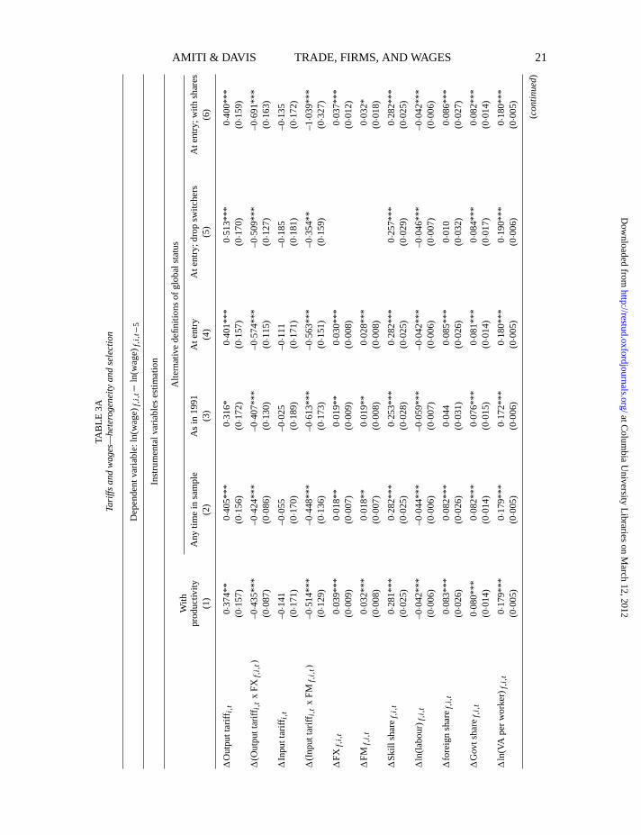
5.2.1. Heterogeneity and selection. A potential concern with the results is that the firm’sdecision to globalize is endogenous, which could lead to biased coefficients. We address this con-cern in a number of different ways in Table 3A, where we estimate the equations in five-perioddifferences using IV estimation, as in Table 2. First, we consider that changes in productivitycould affect the decision to import and export and its omission could bias the estimates, thus,we include value added per worker in Column 1 of Table 3A. As expected, labour productivityhas a significant positive effect on wages, but the coefficients on the tariff terms are very closeto those in our baseline regressions (see Column 4 of Table 2B).

Next, we fix the set of firms used to calculate the interaction terms according to three differentcriteria and show the results are robust.24 By fixing the set of exporters and importers, we ensurethat the coefficient on the interactive terms are not driven by compositional changes into and outof exporting or importing. In Column 2, we define an exporter as a firm that exported at any timeduring the sample period, and an importer as a firm that imported at any time during the sample.In Column 3, we fix the global status as reported in 1991, and in Column 4, we fix the globalstatus at the point the firm enters the sample. The results are robust to all of these alternativespecifications. Although we keep the set of firms interacted with tariffs fixed, we need to controlfor the fact that all firms may actually have changes in import and export status over the sampleperiod, otherwise, we would suffer omitted variable bias. In Column 5, as well as fixing thefirm’s global status at entry, we also drop any firm that changes its global status, so the changein FX and change in FM terms now drop out. Again, we see that the results are robust to thisspecification. In Column 6, we show that the results are also robust to fixing the import andexportsharesat entry.

Even after accounting for the changing global status, there is a potential concern that exit outof production could be biasing the results given that low-productivity firms are more likely toexit. To address this potential concern, we use a two-stage Heckman correction, which requiresa variable to affect the exit decision but not the level of wages. Given that our model assumes an

23. For example,Revenga(1997) finds that on average, a fall in output tariffs reduced wages in Mexico but doesnot allow for an interaction effect for exporters.

24. We would like to thank an anonymous referee for suggesting this approach.

at Colum

bia University L



ownloaded from


“rdr016” — 2012/1/31 — 19:28 — page 21 — #21


TAB

LE3A

Tariffs

an

dw

age

s—h

ete

roge

ne

itya

nd

sele

ctio

n

Dep

ende

ntvar

iabl

e:ln

(wag

e) f,i,t−

ln(w

age)

f,i,

t−5

Inst

rum

enta

lvaria

bles

estim

atio

n

With

Alte

rnat

ive

defin

ition

sof

glob

alst

atus

prod

uctiv

ityA

nytim

ein

sam

ple

As

in19

91A

tent

ryA

tent

ry;d

rop

switc

hers

Ate

ntry

;with

shar

es(1

)(2

)(3

)(4

)(5

)(6

)

1O

utpu

ttar

iffi,

t0∙

374*

*0∙

405*

**0∙

316*

0∙40

1***

0∙51

3***

0∙40

0***

(0∙1

57)

(0∙1

56)

(0∙1

72)

(0∙1

57)

(0∙1

70)

(0∙1

59)

1(O

utpu

ttar

iffi,

tx

FX

f,i,

t)–0

∙435

***

–0∙4

24**

*–0

∙407

***

–0∙5

74**

*–0

∙509

***

–0∙6

91**

*(0

∙087

)(0∙0

86)

(0∙1

30)

(0∙1

15)

(0∙1

27)

(0∙1

63)

1In

putt

ariff

i,t

–0∙1

41–0

∙055

–0∙0

25–0

∙111

–0∙1

85–0

∙135

(0∙1

71)

(0∙1

70)

(0∙1

89)

(0∙1

71)

(0∙1

81)

(0∙1

72)

1(I

nput

tarif

f i,t

xF

Mf,

i,t)

–0∙5

14**

*–0

∙448

***

–0∙6

13**

*–0

∙563

***

–0∙3

54**

–1∙0

39**

*(0

∙129

)(0∙1

36)

(0∙1

73)

(0∙1

51)

(0∙1

59)

(0∙3

27)

1F

Xf,

i,t

0∙03

9***

0∙01

8**

0∙01

9**

0∙03

0***

0∙03

7***

(0∙0

09)

(0∙0

07)

(0∙0

09)

(0∙0

08)

(0∙0

12)

1F

Mf,

i,t

0∙03

2***

0∙01

8**

0∙01

9**

0∙02

8***

0∙03

2*(0

∙008

)(0∙0

07)

(0∙0

08)

(0∙0

08)

(0∙0

18)

1S

kill

shar

e f,i,t

0∙28

1***

0∙28

2***

0∙25

3***

0∙2

82**

*0∙

257*

**0∙

282*

**(0

∙025

)(0∙0

25)

(0∙0

28)

(0∙0

25)

(0∙0

29)

(0∙0

25)

1ln

(labo

ur) f

,i,t

–0∙0

42**

*–0

∙044

***

–0∙0

59**

*–0

∙042

***

–0∙0

46**

*–0

∙042

***

(0∙0

06)

(0∙0

06)

(0∙0

07)

(0∙0

06)

(0∙0

07)

(0∙0

06)

1fo

reig

nsh

are f,

i,t

0∙08

3***

0∙08

2***

0∙04

40∙

085*

**0∙

010

0∙08

6***

(0∙0

26)

(0∙0

26)

(0∙0

31)

(0∙0

26)

(0∙0

32)

(0∙0

27)

1G

ovts

hare

f,i,

t0∙

080*

**0∙

082*

**0∙

076*

**0∙0

81**

*0∙

084*

**0∙

082*

**(0

∙014

)(0∙0

14)

(0∙0

15)

(0∙0

14)

(0∙0

17)

(0∙0

14)

1ln

(VA

per

wor

ker)

f,i,

t0∙

179*

**0∙

179*

**0∙

172*

**0∙1

80**

*0∙

190*

**0∙

180*

**(0

∙005

)(0∙0

05)

(0∙0

06)

(0∙0

05)

(0∙0

06)

(0∙0

05)

(co

ntin

ue

d)

at Colum

bia University L



ownloaded from


“rdr016” — 2012/1/31 — 19:28 — page 22 — #22


TAB

LE3A

Co

ntin

ue

d

Dep

ende

ntvar

iabl

e:ln

(wag

e) f,i,t−

ln(w

age)

f,i,

t−5

Inst

rum

enta

l varia

bles

estim

atio

n

With

Alte

rnat

ive

defin

ition

sof

glob

alst

atus

prod

ucti v

ityA

nytim

ein

sam

ple

As

in19

91A

tent

ryA

tent

ry;d

rop

switc

hers

Ate

ntry

;with

shar

es(1

)(2

)(3

)(4

)(5

)(6

)

J oin

tSig

nific

ance

test

sH

o:su

mof

coef

ficie

nts

onta

riffv

aria

bles

equa

lsze

ro

Out

putt

ariff

s–0

∙060

–0∙0

19–0

∙092

–0∙1

730∙

004

–0∙2

92*

(0∙1

48)

(0∙1

43)

(0∙1

58)

(0∙1

53)

(0∙1

76)

(0∙1

78)

Inpu

ttar

iffs

–0∙6

55**

*–0

∙504

***

–0∙6

37**

*–0

∙674

***

–0∙5

39**

*–1

∙175

***

(0∙2

05)

(0∙1

20)

(0∙2

37)

(0∙2

15)

(0∙2

21)

(0∙3

55)

Han

senJ

stat

istic

3∙19

3∙08

1∙89

2∙82

0∙57

2∙36

p-v

alue

0∙20

0∙21

0∙39

0∙24

0∙75

0∙31

Obs

erv a

tions

50,4

8450

,484

38,3

3550

,484

38,2

7550

,484

No

tes:

Rob

usts

tand

ard

erro

rsin

pare

nthe

ses;

*si

gnifi

cant

at10

%;*

*si

gnifi

cant

at5%

;***

sign

ifica

ntat

1%.I

nstr

umen

tsin

clud

e19

91in

dust

rysk

illsh

are,

1991

indu

stry

skill

shar

ein

tera

cted

with

five-

perio

dla

gged

expo

rtdu

mm

y,19

91in

putt

ariff

leve

l,19

91in

putt

ariff

leve

lint

erac

ted

with

five-

perio

dla

gged

impo

rtdu

mm

y,ex

clus

ion

dum

my

=1

ifte

nor

mor

eH

Sni

ne-d

igit

prod

ucts

excl

uded

with

ina

five-

digi

tin

dust

ryco

defr

omco

mm

itmen

tto

redu

cebo

und

tarif

fsto

40%

,an

dno

n-ta

riff

dum

my

=1

ifte

nor

mor

eH

Sni

ne-d

igit

prod

uct

code

sw

ere

subj

ectt

ono

n-ta

riffb

arrie

rs.A

llsp

ecifi

catio

nspa

ssth

ew

eak

inst

rum

entt

estw

ithF

-sta

tsov

er80

0.A

llth

ees

timat

ions

incl

ude

loca

tion-

year

fixed

effe

cts.

at Colum

bia University L



ownloaded from


“rdr016” — 2012/1/31 — 19:28 — page 23 — #23


TAB

LE3B

Tariffs

an

dw

age

s—h

ete

roge

ne

itya

nd

sele

ctio

n

Dep

ende

ntvar

iabl

e:ln

(wag

e) f,i,t

base

line

1st

stag

e pro

bit

Hec

kman

hete

roge

neity

non-

para

met

ricW

ithex

it1s

tst

age

2nd

stag

e

(1)

(2)

(3)

(4)

(5)

(6)

(7)

Out

putt

ariff

i,t

0∙02

10∙

355*

*0∙

011

0∙00

60∙

462*

**0∙0

160∙

015

(0∙0

45)

(0∙1

69)

(0∙0

49)

(0∙0

49)

(0∙1

70)

(0∙0

48)

(0∙0

45)

Out

putt

ariff

i,t

xF

Xf,

i,t

–0∙0

96**

*–0

∙095

**–0

∙089

**–0

∙100

**–0

∙091

**(0

∙043

)(0

∙044

)(0

∙043

)(0

∙049

)(0

∙043

)

Inpu

ttar

iffi,

t0∙

120

–1∙3

32**

*0∙

159

0∙17

4–1

∙372*

**0∙1

770∙

124

(0∙0

99)

(0∙4

63)

(0∙1

23)

(0∙1

23)

(0∙4

54)

(0∙1

32)

(0∙0

98)

Inpu

ttar

iffi,

tx

FM

f,i,

t–0

∙385

***

–0∙3

82**

*–0

∙368

***

–0∙4

12**

*–0

∙370

***

(0∙0

83)

(0∙0

81)

(0∙0

82)

(0∙0

10)

(0∙0

83)

Ski

llsh

are f

,i,t

0∙29

7***

–0∙2

02**

*0∙

300*

**0∙3

01**

*–0

∙139

0∙30

4***

0∙29

6***

(0∙0

21)

(0∙0

44)

(0∙0

22)

(0∙0

22)

(0∙1

02)

(0∙0

21)

(0∙0

21)

ln(la

bour

) f,i,t

–0∙0

68**

*0∙

125*

**–0

∙072

***

–0∙0

74**

*–0

∙076

***

–0∙0

70**

*(0

∙006

)(0

∙007

)(0

∙007

)(0

∙007

)(0

∙007

)(0

∙006

)

ln(V

Ape

rw

orke

r)f,

i,t

0∙14

3***

0∙02

8***

0∙14

2***

0∙1

42**

*0∙1

42**

*0∙

142*

**(0

∙004

)(0

∙006

)(0

∙004

)(0

∙004

)(0

∙004

)(0

∙004

)

Age

f,i,

t0∙

004*

**–0

∙000

2–0

∙000

4–0

∙000

2(0

∙001

)(0

∙000

4)(0∙0

004)

(0∙0

004)

Age

f,i,

tx

Fin

ance

depe

nden

ce i,t–0

∙004

***

0∙00

010∙0

003

–0∙00

3**

–0∙0

0004

(0∙0

01)

(0∙0

007)

(0∙0

007)

(0∙00

1)(0∙0

008)

(co

ntin

ue

d)

at Colum

bia University L



ownloaded from


“rdr016” — 2012/1/31 — 19:28 — page 24 — #24


TAB

LE3B

Co

ntin

ue

d

Dep

ende

nt var

iabl

e:ln

(wag

e) f,i,t

base

line

1st

stag

e pro

bit

Hec

kman

hete

roge

neity

nonp

aram

etric

With

exit

1st

stag

e2n

dst

age

(1)

(2)

(3)

(4)

(5)

(6)

(7)

Exi

t f,i,t

=1

if–0

∙043

***

exit

int+

1(0

∙006

)

IMR

f,i,

t–0

∙934

***

(0∙2

56)

Ser

iest

erm

s:p-

valu

esfr

omF

-tes

ts

zhat

f,i,

t(3

rdor

der)

0∙00

0***

Age

f,i,

t(4

thor

der)

0∙00

4***

ln(V

Ape

rw

orke

r)f,

i,t

(3r d

orde

r)0∙

000*

**ln

(labo

ur) f

,i,t

0∙00

0***

Inte

ract

iont

erm

s0∙

000*

**P

rope

nsity

f,i,

t(3

rdor

der)

0∙00

0***

J oin

tsig

nific

ance

test

sH

o:su

mof

coef

ficie

nts

onta

riffv

aria

bles

equa

lsze

ro

Out

putt

ariff

–0∙07

4–0

∙084

–0∙08

3–0

∙084

–0∙0

75(0

∙056

)(0∙0

63)

(0∙0

62)

(0∙0

61)

(0∙0

56)

Inpu

ttar

iff–0

∙264

**–0

∙223

*–0

∙194

–0∙23

5*–0

∙246

**(0

∙116

)(0∙1

32)

(0∙1

34)

0∙14

2(0∙1

15)

Obs

erva

tions

109,

302

125,

962

109,

302

109,

302

125,

962

107,

270

109,

302

Adj

uste

dR2

0∙86

0∙03

0∙86

0∙86

0∙05

0∙85

0∙86

No

tes:

Rob

ust

stan

dard

erro

rsin

pare

nthe

ses;

*si

gnifi

cant

at10

%;

**si

gnifi

cant

at5%

;**

*si

gnifi

cant

at1%

.S

tand

ard

erro

rsin

Col

umns

3,4,

and

6ha

vebe

enbo

otst

rapp

edw

ith20

0re

petit

ions

.All

the

estim

atio

nsal

soin

clud

eF

X,F

M,f

orei

gnsh

are,

and

gove

rnm

ents

hare

butt

heco

effic

ient

sar

esu

ppre

ssed

tosa

vesp

ace.

The

top

and

botto

mon

epe

rcen

tiles

ofth

epr

open

sity

mea

sure

have

been

trim

med

.All

estim

atio

nsha

velo

catio

n-ye

aref

fect

san

dfir

m-fi

xed

effe

cts

exce

ptth

efir

st-s

tage

prob

itsin

Col

umns

2an

d5,

whi

chin

clud

eye

aran

din

dust

ryef

fect

s.

at Colum

bia University L



ownloaded from


“rdr016” — 2012/1/31 — 19:28 — page 25 — #25


exogenous rate of firm death, we draw on other related models to find an appropriate variable thatmeets the exclusion restriction.Hopenhayn(1992) shows that the rate of survival is higher forolder firms. AndChaney(2005) shows how financial constraints can affect entry and exit intothe export market. The model assumes that firms only face liquidity constraints for accessingforeign markets, but one could easily imagine that financial constraints also apply to entry andexit decisions in the domestic market. Building on this intuition, we use an industry measure ofexternal financial dependence, defined as the share of capital expenditures not funded by cashflows for the median U.S. firm in the 1980’s, fromRajan and Zingales(1998).25 We use thesetwo measures in the first-stage selection equation.

The Heckman correction is more straightforward in a levels equation where exit is more eas-ily defined than in the long-difference specification where being in the sample would have to bedefined as present in periodt andt −5. Thus, in Column 1 of Table 3B, we first show that ourfive-period differenced results also hold in a levels equation. In Column 2, we present the first-stage probit results, where the dependent variable is equal to one if the firm is in the sample thatyear and equal to zero in the year the firm exits. We model the probability of being in the sampleas a function of the variables used in the second stage, lagged one period, year-fixed effects andindustry-fixed effects. The results show that the probability of being in the sample is increasing inoutput tariffs, as firms are protected from import competition; decreasing in input tariffs, as highinput tariffs make it more costly to produce; and increasing in value added per worker. The finan-cial dependence variable on its own would drop out because this measure is time invariant due tothe industry-fixed effects. Thus, we interact it with the firm’s age that is firm-specific and time-varying. That is, the age variable is constructed by subtracting the year that the firm started op-erations in a province from the sample year. As expected, the probability of being in the sampleincreases with the age of the firm but this is offset if the firm is in an industry that is rela-tively more dependent on external finance. We construct the inverse mills ratio (IMR) from thisselection equation and include it in the second-stage Heckman correction in Column 3. As ex-pected, the age variables are both insignificant in the second stage, thus meeting the exclusionrestriction. Moreover, this Heckman correction leaves the results unchanged (compare Columns1 and 3 of Table 3B), which implies that selection is not biasing our results.26As shown inHelpman, Melitz and Rubinstein(2008), even if there is no selection bias, there may be a het-erogeneity bias, which could arise from the changing global status of firms. We address this po-tential concern following their methodology and include a third-order polynomial ofz

∗≡ z∗ +

IMR, wherez∗ is defined as the inverse cumulative distribution of the fitted values from the first-stage probit. Column 4 shows that while thez terms are significant, they leave the point estimateson the tariff terms unchanged, indicating that our results are not driven by heterogeneity bias.

In Columns 5 and 6, we re-estimate the two-stage Heckman correction using a non-parametricapproach as inDas, Newey and Vella(2003) to allow for the functional form of regressionsand the disturbance distributions to be unknown.27 We use the Akaike information criterion toquery the appropriate order of the polynomial expansion in the first stage as well as to determinethe appropriate order of polynomial of the propensity score variable in the second stage. FromColumns 5 and 6, we see that the results are robust to this non-parametric correction.

Finally, in Column 7, we control for exit and show this has no effect on our main results.The exit dummy variable equals one if the firm exits in periodt + 1. The coefficient on the

25. These data are at the three- and four-digit ISIC level and comprise 36 industries.26. Note that we restrict the sample size in Columns 1 to be the same as the Heckman correction equation in order

to assess the potential selection bias. The Heckman equation has fewer observations than the full sample because theselection equation includes firm specific one-period lagged regressors.

27. See alsoBecker and Muendler(2010) for an application.

at Colum

bia University L



ownloaded from


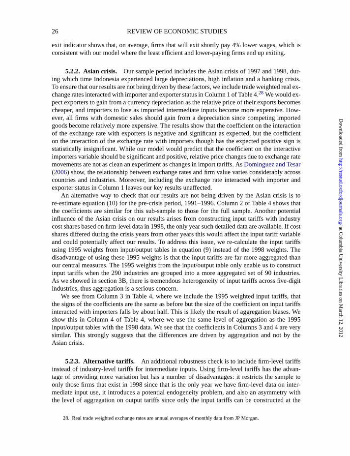
“rdr016” — 2012/1/31 — 19:28 — page 26 — #26


exit indicator shows that, on average, firms that will exit shortly pay 4% lower wages, which isconsistent with our model where the least efficient and lower-paying firms end up exiting.

5.2.2. Asian crisis. Our sample period includes the Asian crisis of 1997 and 1998, dur-ing which time Indonesia experienced large depreciations, high inflation and a banking crisis.To ensure that our results are not being driven by these factors, we include trade weighted real ex-change rates interacted with importer and exporter status in Column 1 of Table 4.28 We would ex-pect exporters to gain from a currency depreciation as the relative price of their exports becomescheaper, and importers to lose as imported intermediate inputs become more expensive. How-ever, all firms with domestic sales should gain from a depreciation since competing importedgoods become relatively more expensive. The results show that the coefficient on the interactionof the exchange rate with exporters is negative and significant as expected, but the coefficienton the interaction of the exchange rate with importers though has the expected positive sign isstatistically insignificant. While our model would predict that the coefficient on the interactiveimporters variable should be significant and positive, relative price changes due to exchange ratemovements are not as clean an experiment as changes in import tariffs. AsDominguez and Tesar(2006) show, the relationship between exchange rates and firm value varies considerably acrosscountries and industries. Moreover, including the exchange rate interacted with importer andexporter status in Column 1 leaves our key results unaffected.

An alternative way to check that our results are not being driven by the Asian crisis is tore-estimate equation (10) for the pre-crisis period, 1991–1996. Column 2 of Table 4 shows thatthe coefficients are similar for this sub-sample to those for the full sample. Another potentialinfluence of the Asian crisis on our results arises from constructing input tariffs with industrycost shares based on firm-level data in 1998, the only year such detailed data are available. If costshares differed during the crisis years from other years this would affect the input tariff variableand could potentially affect our results. To address this issue, we re-calculate the input tariffsusing 1995 weights from input/output tables in equation (9) instead of the 1998 weights. Thedisadvantage of using these 1995 weights is that the input tariffs are far more aggregated thanour central measures. The 1995 weights from the input/output table only enable us to constructinput tariffs when the 290 industries are grouped into a more aggregated set of 90 industries.As we showed in section 3B, there is tremendous heterogeneity of input tariffs across five-digitindustries, thus aggregation is a serious concern.

We see from Column 3 in Table 4, where we include the 1995 weighted input tariffs, thatthe signs of the coefficients are the same as before but the size of the coefficient on input tariffsinteracted with importers falls by about half. This is likely the result of aggregation biases. Weshow this in Column 4 of Table 4, where we use the same level of aggregation as the 1995input/output tables with the 1998 data. We see that the coefficients in Columns 3 and 4 are verysimilar. This strongly suggests that the differences are driven by aggregation and not by theAsian crisis.

5.2.3. Alternative tariffs. An additional robustness check is to include firm-level tariffsinstead of industry-level tariffs for intermediate inputs. Using firm-level tariffs has the advan-tage of providing more variation but has a number of disadvantages: it restricts the sample toonly those firms that exist in 1998 since that is the only year we have firm-level data on inter-mediate input use, it introduces a potential endogeneity problem, and also an asymmetry withthe level of aggregation on output tariffs since only the input tariffs can be constructed at the

28. Real trade weighted exchange rates are annual averages of monthly data from JP Morgan.

at Colum

bia University L



ownloaded from


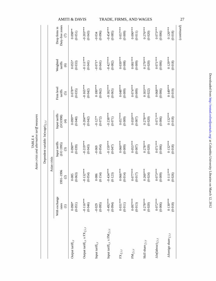
“rdr016” — 2012/1/31 — 19:28 — page 27 — #27


TAB

LE4

Asi

an

cris

isa

nd

alte

rna

tive

tariff

me

asu

re

s

Dep

ende

ntvar

iabl

e:ln

(wag

e) f,i,t

Asi

ancr

isis

With

exch

ange

Inpu

ttar

iffs

Inpu

ttar

iffs

Firm

leve

lW

eigh

ted

Dro

pfir

ms

inra

tes

1991

–199

6(I

/O19

95)

(I/O

1998

)ta

riffs

tarif

fsD

uty-

free

zone

s(1

)(2

)(3

)(4

)(5

)(6

)(7

)

Out

putt

ariff

i,t

0∙09

0*0∙

085

0∙09

0**

0∙09

9**

0∙07

8**

0∙05

5*0∙

098*

*(0

∙051

)(0∙0

63)

(0∙0

39)

(0∙0

40)

(0∙0

35)

(0∙0

33)

(0∙0

51)

Out

putt

ariff

i,t

xF

Xf,

i,t

–0∙1

16**

*–0

∙132

***

–0∙2

19**

*–0

∙204

***

–0∙1

65**

*–0

∙111

***

–0∙2

03**

*(0

∙046

)(0∙0

54)

(0∙0

43)

(0∙0

42)

(0∙0

42)

(0∙0

41)

(0∙0

43)

Inpu

ttar

iffi,

t–0

∙029

0∙08

6–0

∙069

–0∙1

27*

0∙18

0***

–0∙0

71*

–0∙0

34(0

∙095

)(0∙1

54)

(0∙0

54)

(0∙0

72)

(0∙0

62)

(0∙0

41)

(0∙0

96)

Inpu

ttar

iffi,

tx

FM

f,i,

t–0

∙492

***

–0∙4

34**

*–0

∙159

***

–0∙2

38**

*–0

∙302

***

–0∙4

27**

*–0

∙454

***

(0∙0

94)

(0∙1

23)

(0∙0

47)

(0∙0

71)

(0∙0

65)

(0∙0

82)

(0∙0

85)

FX

f,i,

t0∙

031*

**0∙

066*

**0∙

060*

**0∙0

57**

*0∙

048*

**0∙

039*

**0∙0

57**

*(0

∙011

)(0∙0

14)

(0∙0

09)

(0∙0

09)

(0∙0

09)

(0∙0

08)

(0∙0

09)

FM

f,i,

t0∙

097*

**0∙

077*

**0∙

055*

**0∙0

59**

*0∙

074*

**0∙

081*

**0∙0

90**

*(0

∙013

)(0∙0

17)

(0∙0

07)

(0∙0

07)

(0∙0

09)

(0∙0

09)

(0∙0

11)

Ski

llsh

are f

,i,t

0∙27

8***

0∙26

0***

0∙27

8***

0∙2

78**

*0∙

303*

**0∙

279*

**0∙2

76**

*(0

∙020

)(0∙0

24)

(0∙0

20)

(0∙0

20)

(0∙0

22)

(0∙0

20)

(0∙0

20)

1ln

(labo

ur) f

,i,t

0∙07

2***

0∙07

3***

0∙07

1***

0∙0

71**

*0∙

068*

**0∙

071*

**0∙0

73**

*(0

∙006

)(0∙0

09)

(0∙0

06)

(0∙0

06)

(0∙0

06)

(0∙0

06)

(0∙0

06)

1fo

reig

nsh

are f,

i,t

0∙13

0***

0∙11

1***

0∙13

2***

0∙1

32**

*0∙

149*

**0∙

129*

**0∙1

26**

*(0

∙018

)(0∙0

26)

(0∙0

18)

(0∙0

18)

(0∙0

19)

(0∙0

18)

(0∙0

18)

(co

ntin

ue

d)

at Colum

bia University L



ownloaded from


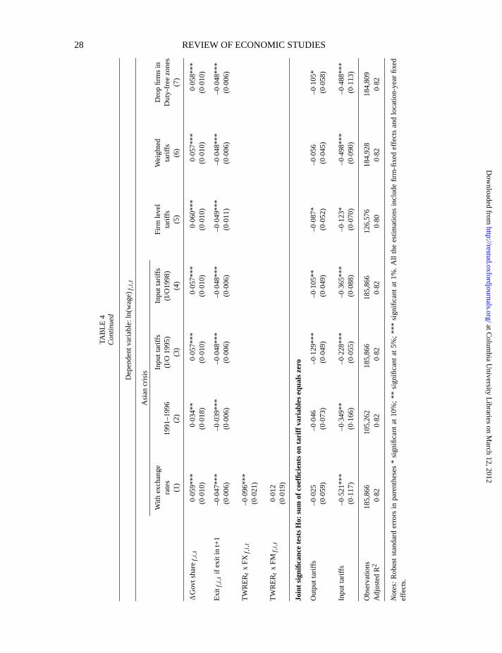
“rdr016” — 2012/1/31 — 19:28 — page 28 — #28


TAB

LE4

Co

ntin

ue

d

Dep

ende

ntvar

iabl

e:ln

(wag

e) f,i,t

Asi

ancr

isis

With

exch

ange

Inpu

ttar

iffs

Inpu

ttar

iffs

Firm

leve

lW

eigh

ted

Dro

pfir

ms

inra

tes

1991

–199

6(I

/O19

95)

(I/O

1998

)ta

riffs

tarif

fsD

uty-

free

zone

s(1

)(2

)(3

)(4

)(5

)(6

)(7

)

1G

ovts

hare

f,i,

t0∙

059*

**0∙

034*

*0∙

057*

**0∙

057*

**0∙

060*

**0∙

057*

**0∙0

58**

*(0

∙010

)(0

∙018

)(0

∙010

)(0

∙010

)(0

∙010

)(0

∙010

)(0

∙010

)

Exi

t f,i,t

ifex

itin

t+1

–0∙0

47**

*–0

∙039

***

–0∙0

48**

*–0

∙048

***

–0∙0

49**

*–0

∙048

***

–0∙0

48**

*(0

∙006

)(0

∙006

)(0

∙006

)(0

∙006

)(0

∙011

)(0

∙006

)(0

∙006

)

TW

RE

R tx

FX

f,i,

t–0

∙096

***

(0∙0

21)

TW

RE

R tx

FM

f,i,

t0∙

012

(0∙0

19)

Join

tsig

nific

ance

test

sH

o:su

mof

coef

ficie

nts

onta

riffv

aria

bles

equa

lsze

ro

Out

putt

ariff

s–0

∙025

–0∙04

6–0

∙129

***

–0∙1

05**

–0∙0

87*

–0∙0

56–0

∙105

*(0

∙059

)(0

∙073

)(0

∙049

)(0

∙049

)(0

∙052

)(0

∙045

)(0

∙058

)

Inpu

ttar

iffs

–0∙5

21**

*–0

∙349

**–0

∙228

***

–0∙3

65**

*–0

∙123

*–0

∙498

***

–0∙4

88**

*(0

∙117

)(0

∙166

)(0

∙055

)(0

∙088

)(0

∙070

)(0

∙090

)(0

∙113

)

Obs

erva

tions

185,

866

105,

262

185,

866

185,

866

126,

576

184,

928

184,

809

Adj

uste

dR2

0∙82

0∙82

0∙82

0∙82

0∙80

0∙82

0∙82

No

tes:

Rob

ust

stan

dard

erro

rsin

pare

nthe

ses

*si

gnifi

cant

at10

%;

**si

gnifi

cant

at5%

;**

*si

gnifi

cant

at1%

.A

llth

ees

timat

ions

incl

ude

firm

-fixe

def

fect

san

dlo

catio

n-ye

arfix

edef

fect

s.

at Colum

bia University L



ownloaded from


“rdr016” — 2012/1/31 — 19:28 — page 29 — #29


firm level. Nevertheless, we check the robustness of our industry-level input tariffs by replacingit with firm-level tariffs in Column 5 of Table 4 and we see that main conclusions are unaf-fected.

Another concern is the choice of weights in constructing the five-digit industry tariffs fromthe underlying HS nine-digit tariff data. We use simple averages in our main estimations, butwe present estimates of the effect of import weighted tariff cuts on wages using the Fisherindex, as a robustness check in Column 6 of Table 4.29 Theseresults are similar to those withsimple average tariffs except that the size of the coefficients on the output tariff variables is a bitsmaller.

Finally, there may be a concern arising from Indonesia operating duty-free zones, whichallows firms to import inputs without paying any tariffs if their output is for export. If a firmwas already able to import duty-free inputs, then cuts in input tariffs should not be of benefitto them and in fact could hinder their performance due to the competition effect of other firmsbeing able to access lower-cost imported inputs. To ensure that this does not bias our coefficients,we omit all firms that operate in a duty-free zone. Column 7 shows that the results are unaffectedby dropping these observations.

5.3. Mechanisms

The empirics establish a robust relation between tariff changes, modes of globalization and av-erage firm-level wages. We develop this within a theoretical framework in which tariff changes,mediated by modes of globalization, lead to changes in firm profitability, and these in turn affectwages. It is worth noting, though, that the link between tariff changes and wages could be viewedthrough the lenses of a variety of models. Our approach has focused on firm heterogeneity andabstracted from worker heterogeneity in wage formation and changes. However, it is possiblethat globalized firms attract a different type of worker; respond to tariff changes by adjustingthe composition of workers or adjust product quality, and hence also change either their mixof workers or their demands on workers. Examples of these alternative models includeYeaple(2005) andVerhoogen(2008). Any data set will have limitations, as does ours, so we will goas far as we can in demonstrating the robustness of our results to controls for these alternativeinterpretations.

A first question concerns the role of worker vs. firm heterogeneity in wage determina-tion. Early studies stressed the importance of individual worker heterogeneity; however, morerecent results have underscored the role of firm heterogeneity, particularly concerning changesin wages.Abowd, Kramarz and Margolis(1999), shows that worker heterogeneity is more im-portant than firm heterogeneity in determining wages in French data. However, a subsequentpaper byAbowd, Creecy and Kramarz(2002) shows that using an exact solution, the correla-tion between worker and firm effects is negative, in contrast to the earlier finding of a positivecorrelation. In comparing the results for France and for the State of Washington, the study findsthat the worker and firm components have equal importance. Recent work byFrias, Kaplanand Verhoogen(2009) uses matched employer–employee data for Mexico. They show that two-thirds of the higher level of wages can be explained by firm heterogeneity; that nearly all thewithin-industry wage changes can be explained by firm differences; and none of the changes re-flect changes in skill composition. Since matched firm-worker data are unavailable for Indonesia,we are unable do this decomposition. Still, the literature does establish that there is potentially a

29. The results are the same using 1991 or 2000 weights. We were unable to get imports at the HS nine-digit level,so the import-weighted five-digit ISIC tariffs are constructed by first taking the simple mean of the HS nine-digit to HSsix-digit, then weighting the HS six-digit tariffs by the import shares.

at Colum

bia University L



ownloaded from


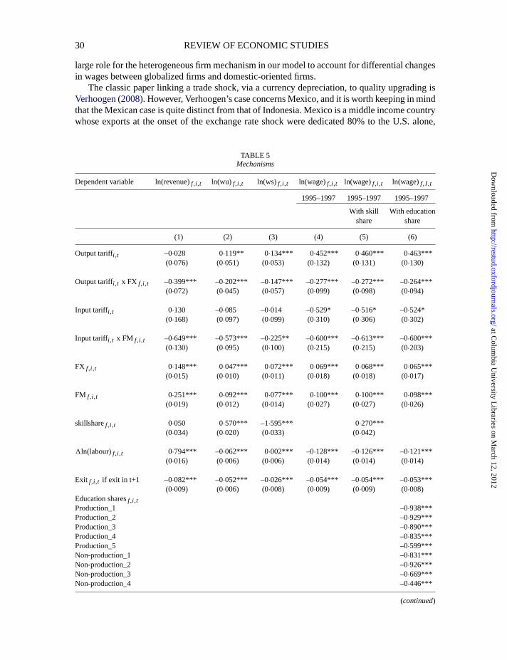
“rdr016” — 2012/1/31 — 19:28 — page 30 — #30


large role for the heterogeneous firm mechanism in our model to account for differential changesin wages between globalized firms and domestic-oriented firms.

The classic paper linking a trade shock, via a currency depreciation, to quality upgrading isVerhoogen(2008). However, Verhoogen’s case concerns Mexico, and it is worth keeping in mindthat the Mexican case is quite distinct from that of Indonesia. Mexico is a middle income countrywhose exports at the onset of the exchange rate shock were dedicated 80% to the U.S. alone,

TABLE 5Mechanisms

Dependentvariable ln(revenue)f,i,t ln(wu) f,i,t ln(ws) f,i,t ln(wage)f,i,t ln(wage)f,i,t ln(wage)f,I ,t

1995–1997 1995–1997 1995–1997

With skill With educationshare share

(1) (2) (3) (4) (5) (6)

Outputtariffi,t –0∙028 0∙119** 0∙134*** 0 ∙452*** 0 ∙460*** 0 ∙463***(0∙076) (0∙051) (0∙053) (0∙132) (0∙131) (0∙130)

Output tariffi,t x FX f,i,t –0∙399*** –0∙202*** –0∙147*** –0∙277*** –0∙272*** –0∙264***(0∙072) (0∙045) (0∙057) (0∙099) (0∙098) (0∙094)

Input tariffi,t 0∙130 –0∙085 –0∙014 –0∙529* –0∙516* –0∙524*(0∙168) (0∙097) (0∙099) (0∙310) (0∙306) (0∙302)

Input tariffi,t x FM f,i,t –0∙649*** –0∙573*** –0∙225** –0∙600*** –0∙613*** –0∙600***(0∙130) (0∙095) (0∙100) (0∙215) (0∙215) (0∙203)

FX f,i,t 0∙148*** 0∙047*** 0 ∙072*** 0 ∙069*** 0 ∙068*** 0 ∙065***(0∙015) (0∙010) (0∙011) (0∙018) (0∙018) (0∙017)

FM f,i,t 0∙251*** 0∙092*** 0 ∙077*** 0 ∙100*** 0 ∙100*** 0 ∙098***(0∙019) (0∙012) (0∙014) (0∙027) (0∙027) (0∙026)

skillsharef,i,t 0∙050 0∙570*** –1∙595*** 0 ∙270***(0∙034) (0∙020) (0∙033) (0∙042)

1ln(labour)f,i,t 0∙794*** –0∙062*** 0 ∙002*** –0∙128*** –0∙126*** –0∙121***(0∙016) (0∙006) (0∙006) (0∙014) (0∙014) (0∙014)

Exit f,i,t if exit in t+1 –0∙082*** –0∙052*** –0∙026*** –0∙054*** –0∙054*** –0∙053***(0∙009) (0∙006) (0∙008) (0∙009) (0∙009) (0∙008)

Education sharesf,i,tProduction_1 –0∙938***Production_2 –0∙929***Production_3 –0∙890***Production_4 –0∙835***Production_5 –0∙599***Non-production_1 –0∙831***Non-production_2 –0∙926***Non-production_3 –0∙669***Non-production_4 –0∙446***

(continued)

at Colum

bia University L



ownloaded from


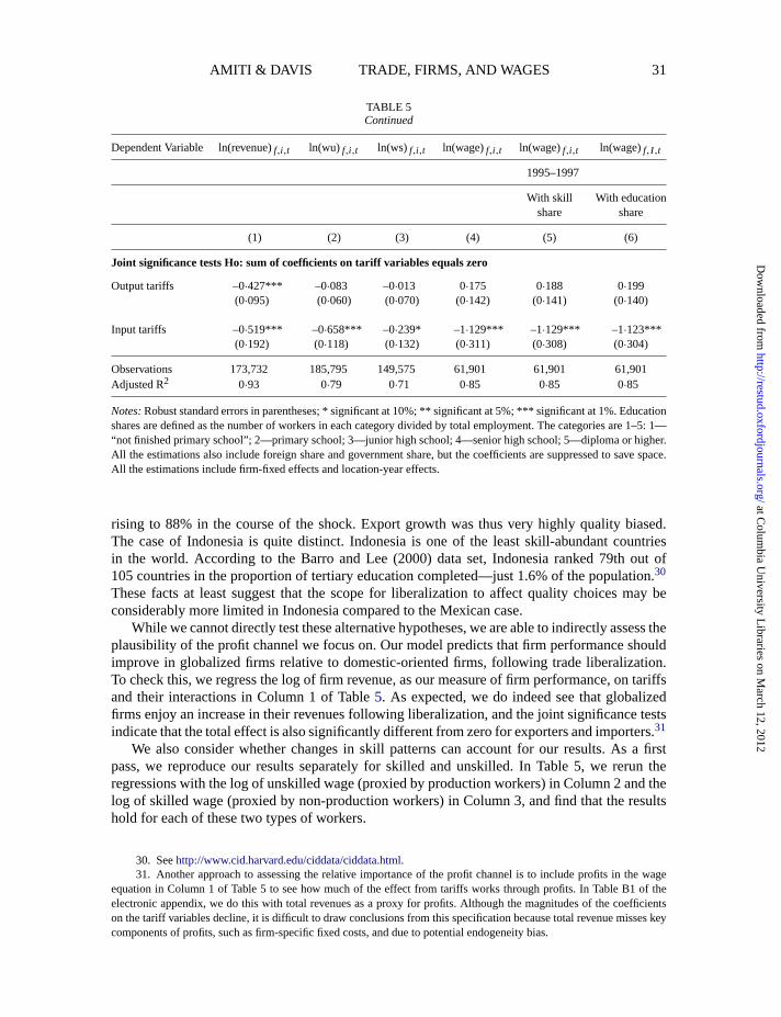
“rdr016” — 2012/1/31 — 19:28 — page 31 — #31


TABLE 5Continued

DependentVariable ln(revenue)f,i,t ln(wu) f,i,t ln(ws) f,i,t ln(wage)f,i,t ln(wage)f,i,t ln(wage)f,I ,t

1995–1997

With skill With educationshare share

(1) (2) (3) (4) (5) (6)

Joint significance tests Ho: sum of coefficients on tariff variables equals zero

Output tariffs –0∙427*** –0∙083 –0∙013 0∙175 0∙188 0∙199(0∙095) (0∙060) (0∙070) (0∙142) (0∙141) (0∙140)

Input tariffs –0∙519*** –0∙658*** –0∙239* –1∙129*** –1∙129*** –1∙123***(0∙192) (0∙118) (0∙132) (0∙311) (0∙308) (0∙304)


Notes:Robust standard errors in parentheses; * significant at 10%; ** significant at 5%; *** significant at 1%. Educationshares are defined as the number of workers in each category divided by total employment. The categories are 1–5: 1—“not finished primary school”; 2—primary school; 3—junior high school; 4—senior high school; 5—diploma or higher.All the estimations also include foreign share and government share, but the coefficients are suppressed to save space.All the estimations include firm-fixed effects and location-year effects.

rising to 88% in the course of the shock. Export growth was thus very highly quality biased.The case of Indonesia is quite distinct. Indonesia is one of the least skill-abundant countriesin the world. According to the Barro and Lee (2000) data set, Indonesia ranked 79th out of105 countries in the proportion of tertiary education completed—just 1.6% of the population.30

Thesefacts at least suggest that the scope for liberalization to affect quality choices may beconsiderably more limited in Indonesia compared to the Mexican case.

While we cannot directly test these alternative hypotheses, we are able to indirectly assess theplausibility of the profit channel we focus on. Our model predicts that firm performance shouldimprove in globalized firms relative to domestic-oriented firms, following trade liberalization.To check this, we regress the log of firm revenue, as our measure of firm performance, on tariffsand their interactions in Column 1 of Table5. As expected, we do indeed see that globalizedfirms enjoy an increase in their revenues following liberalization, and the joint significance testsindicate that the total effect is also significantly different from zero for exporters and importers.31

We also consider whether changes in skill patterns can account for our results. As a firstpass, we reproduce our results separately for skilled and unskilled. In Table 5, we rerun theregressions with the log of unskilled wage (proxied by production workers) in Column 2 and thelog of skilled wage (proxied by non-production workers) in Column 3, and find that the resultshold for each of these two types of workers.

30. Seehttp://www.cid.harvard.edu/ciddata/ciddata.html.31. Another approach to assessing the relative importance of the profit channel is to include profits in the wage

equation in Column 1 of Table 5 to see how much of the effect from tariffs works through profits. In Table B1 of theelectronic appendix, we do this with total revenues as a proxy for profits. Although the magnitudes of the coefficientson the tariff variables decline, it is difficult to draw conclusions from this specification because total revenue misses keycomponents of profits, such as firm-specific fixed costs, and due to potential endogeneity bias.

at Colum

bia University L



ownloaded from

http://www.cid.harvard.edu/ciddata/ciddata.html


“rdr016” — 2012/1/31 — 19:28 — page 32 — #32


While encouraging, we would like to ensure that our results are not driven just by changes inskill composition at the firm level. Although we control for the share of non-production workersin our main specifications, there may still be changes in the share of educated workerswithin thebroader production and non-production categories that could be driving the changes in wages.Information on worker education is not available for the full sample but does exist for threeyears, between 1995 and 1997. There are five different education levels for production workers,ranging from 1 to 5 with 5 being the highest level, and similarly for non-production workers.32

In Column 4 of Table 5, we show that our results hold for these three years of data without anycontrol for skill shares. In Column 5, we show that the results are unchanged if we control forthe share of production workers. And in Column 6, we include controls by education level. Thisincludes ten categories of education in total, with the omitted category being the most educatednon-production workers. We see that all the coefficients on education shares are negative andsignificant, but most importantly they do not change the point estimates on the tariff variables atall. These findings suggest that compositional changes in skill are not driving our results. Whilethe mechanisms identified in our model are not necessarily the whole story, they appear to be arobust component of the link between tariff liberalization and firm wages.

FIGURE 2Modes of globalization and firm-wage changes. The predominance of negative values near the origin indicates that

non-globalizers lose from liberalization, and vice versa for those who globalize via exports or imports

32. The categories are 1–5: 1—“not finished primary school”; 2—primary school; 3—junior high school; 4—senior high school; 5—diploma or higher.

at Colum

bia University L



ownloaded from


“rdr016” — 2012/1/31 — 19:28 — page 33 — #33


5.4. Discussion of results

Since all our estimates include year fixed effects, these will capture an average effect of tradeliberalization on wages. We cannot determine the total effect of trade liberalization on wagesbecause we cannot separately identify the role of tariff cuts on the year effects. Still, relativeto the average, exporters and importers pay higher wages following tariff cuts and domesticoriented firms pay lower wages. This can be seen clearly from Figure2 where we plot thefirm’s predicted change in wage as a function of its import share and export share. We calculatethe firm’s fitted wage, resulting from the change in tariffs over the whole sample period usingcoefficients from Column 5 in Table 2B, for all firms in the sample in 2000 as follows:

1w f = β1 * 1outputtariffi + β2 * 1outputtariffi ∗export sharef

+ β3 * 1input tariff + β4 ∗1input tariffi * import sharef .

We see from Figure2 that firms with negative predicted wages are those that are predominantlydomestic oriented (close to the origin), and those with the large positive predicted wages arethe industries that are large globalizers either with a high-export share or a high-import share(away from the origin). There is large heterogeneity in firm-level wage responses. For example,in the motor vehicle industry, which experienced one of the biggest declines in output tariffs of45 percentage points, the fitted wage change for firms that sell all their output in the domesticmarket and buy all their inputs locally is a fall of 15%. Yet, within the same industry, firms thatexport large shares of their output and import their inputs have a positive fitted wage change of4%. The largest predicted wage gains following tariff cuts were 29% in the toy industry, whichexperienced big cuts in both input and output tariffs, and these were for firms that export all oftheir output and import all of their inputs.

6. CONCLUSIONS

The effect of trade liberalization on wages has generated a vast literature in international eco-nomics. Yet, no prior study has simultaneously accounted for the two most salient empirical factsabout international production to emerge in the last decade. The first fact is firm heterogeneity—large firms are more productive, more likely to export and import, and pay higher wages. Thesecond fact is the prominent role of intermediate trade, distinct from final goods trade. Firm het-erogeneity is the very foundation of our approach to firm-level wages. And theory tells us thatreductions in final and intermediate goods tariffs tend to have opposite signs, so distinguishingtheir impacts is crucial. We incorporate both salient facts in our analysis.

Our theory combines elements ofMelitz (2003) andKasahara and Lapham(2007) with aspecification of fair-wage setting closely related to that ofGrossman and Helpman(2007) . Thisallows us to develop a general equilibrium model with firm heterogeneity, trade in final andintermediate goods, and firm-specific wages. The model predicts that the wage consequencesof liberalization vary qualitatively and quantitatively with the nature and magnitude of firms’global engagement via exports and imports.

We examine the predictions of the model with highly detailed firm-level data for the Indone-sian trade liberalization in the period 1991–2000. Of particular note is that our data allow us toconstruct highly detailed import tariffs on inputs, hence to separate the effects of cuts in inputtariffs from cuts in output tariffs.

The results are strongly supportive of the predictions arising from the theory and stable acrossa wide variety of robustness checks. Introducing firm heterogeneity and a separate impact for

at Colum

bia University L



ownloaded from


“rdr016” — 2012/1/31 — 19:28 — page 34 — #34


input and output tariffs (and their interactions) is crucial to the results. Cuts in output tariffsreduce wages at firms oriented exclusively to the domestic market but raise wages at firms thatexport a sufficient share of their output. Cuts in input tariffs raise wages at firms that importinputs while having an insignificant effect on wages of workers at firms that fail to import.

We would like to highlight a few directions for future work. First, although the results areconsistent with our fair-wage model, the data do not permit us to rule out some role for com-positional shifts within education categories or changes in unobserved worker heterogeneity inthe differential wage responses of globalized and domestically oriented firms. This remains anarea for future research. Second, changes in final and intermediate output tariffs here function asinternational demand and cost shocks. It would be very interesting to investigate whether suchshocks function differently based on domestic or international origin. Third, while we developeda specific mechanism, fair wages, through which the tariff shocks are transmitted to wages, itwould be very interesting to have data with profit measures and more institutional detail thatwould permit a clear contrast between competing theories of the mechanism involved. Fourth,we have not modelled explicitly the role of foreign firms. Doing so and exploring in more detailany contrasts between domestic and foreign firms would be interesting.

TABLE A1Summarystatistics

Levels Five-period differences

Variable Mean Standard deviation Mean Standard deviation

ln(wage)f,i,t 7∙35 0∙80 0∙70 0∙54ln(ws) f,i,t 7∙87 0∙92ln(wu) f,i,t 7∙25 0∙79ln(labour)f,i,t 4∙18 1∙19 0∙01 0∙53Skill sharef,i,t 0∙14 0∙15 0∙00 0∙14Foreign sharef,i,t 0∙04 0∙18 0∙00 0∙11Govt sharef,i,t 0∙02 0∙14 0∙17 0∙40Export sharef,i,t 0∙11 0∙29 –0∙02 0∙28Export sharef,i,t if FX=1 0∙71 0∙33FX f,i,t =1 if exshare>0 0∙15 0∙36 –0∙03 0∙38Import sharef,i,t 0∙09 0∙24 –0∙01 0∙20Import sharef,i,t if FM=1 0∙47 0∙36FM f,i,t =1 if import share>0 0∙19 0∙39 –0∙02 0∙34Exit f,i,t =1 if exit next period 0∙08 0∙28Age f,i,t 12∙67 12∙73Output tariffi,t 0∙17 0∙11 –0∙12 0∙08Input tariffi,t 0∙11 0∙06 –0∙03 0∙08ln(TFP)f,i,t 1∙63 0∙66ln(VA per worker)f,i,t 8∙56 1∙25 0∙67 0∙96ln(revenue)f,i,t 13∙62 2∙06Financial dependence 0∙23 0∙35Production_1f,i,t 0∙08 0∙17Production_2f,i,t 0∙36 0∙29Production_3f,i,t 0∙22 0∙20Production_4f,i,t 0∙19 0∙22Production_5f,i,t 0∙01 0∙03Non-production_1f,i,t 0∙00 0∙03

(continued)

at Colum

bia University L



ownloaded from


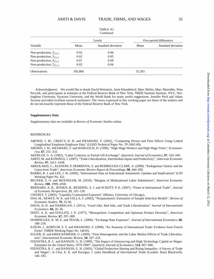
“rdr016” — 2012/1/31 — 19:28 — page 35 — #35


TABLE A1Continued

Levels Five-period differences

Variable Mean Standard deviation Mean Standard deviation

Non-production_2f,i,t 0∙02 0∙06Non-production_3f,i,t 0∙02 0∙05Non-production_4f,i,t 0∙07 0∙09Non-production_5f,i,t 0∙02 0∙04

Observations 185,866 55,393

Acknowledgment. We would like to thank David Weinstein, Amit Khandelwal, Marc Melitz, Marc Muendler, NinaPavcnik, and participants at seminars at the Federal Reserve Bank of New York, NBER Summer Institute, NYU, Not-tingham University, Syracuse University, and the World Bank for many useful suggestions. Jennifer Peck and AdamSacarny provided excellent research assistance. The views expressed in this working paper are those of the authors anddo not necessarily represent those of the Federal Reserve Bank of New York.

Supplementary Data

Supplementary data are available atReview of Economic Studiesonline.

REFERENCES

ABOWD, J. M., CREECY, R. H. and KRAMARZ, F. (2002), “Computing Person and Firm Effects Using LinkedLongitudinal Employer-Employee Data” (LEHD Technical Paper No. TP-2002-09).

ABOWD, J. M., KRAMARZ, F. and MARGOLIS, D. (1999), “High Wage Workers and High Wage Firms”,Economet-rica, 67, 251–333.

AKERLOF, G. A. (1982), “Labor Contracts as Partial Gift Exchange”,Quarterly Journal of Economics, 97, 543–569.AMITI, M. and KONINGS, J. (2007), “Trade Liberalization, Intermediate Inputs and Productivity”,American Economic

Review, 97, 1611–1638.ARKOLAKIS, C., KLENOW, P. DEMIDOVA, S. and RODRIGUEZ-CLARE, A. (2008), “Endogenous Variety and the

Gains from Trade”,American Economic Review Papers & Proceedings, 98, 444–450.BARRO, R. J. and LEE, J. W. (2000), “International Data on Educational Attainment: Updates and Implications” (CID

Working Paper No. 42).BECKER, S. O. and MUENDLER, M. (2010), “Margins of Multinational Labor Substitution”,American Economic

Review, 100, 1999–2030.BERNARD, A. B., JENSEN, B., REDDING, S. J. and SCHOTT, P. K. (2007), “Firms in International Trade”,Journal

of Economic Perspectives, 21, 105–130.CHANEY, T. (2005), “Liquidity Constrained Exporters” (Mimeo, University of Chicago).DAS, M., NEWEY, W. K. and VELLA, F. (2003), “Nonparametric Estimation of Sample Selection Models”,Review of

Economic Studies,70, 33-58.DAVIS, D. R. and HARRIGAN, J. (2011), “Good Jobs, Bad Jobs, and Trade Liberalization”Journal of International

Economics.84, 26–36.DIXIT, A. K. and STIGLITZ, J. E. (1977), “Monopolistic Competition and Optimum Product Diversity”,American

Economic Review, 67, 297–308.DOMINGUEZ, K. M. E. and TESAR, L. (2006), “Exchange Rate Exposure”,Journal of International Economics,68,

188–218.EATON, J., KORTUM, S. S. and KRAMARZ, F. (2008), “An Anatomy of International Trade: Evidence from French

Firms” (NBER Working Paper No. 14610).EGGER, H. and KREICKEMEIER, U. (2009), “Firm Heterogeneity and the Labor Market Effects of Trade Liberaliza-

tion”, International Economic Review, 50, 187–216.FEENSTRA, R. C. and HANSON, G. H. (1999), “The Impact of Outsourcing and High-Technology Capital on Wages:

Estimates for the United States, 1979-1990”,Quarterly Journal of Economics,114, 907–940.FEENSTRA, R. C. and HANSON, G. H. (2003), “Global Production Sharing and Rising Inequality: A Survey of Trade

and Wages”, in Choi, E. K. and Harrigan, J. (eds)Handbook of International Trade(London: Basil Blackwell),146–185.

at Colum

bia University L



ownloaded from


“rdr016” — 2012/1/31 — 19:28 — page 36 — #36


FELBERMAYR, G. J., PRAT, J. and SCHMERER, H-J. (2011), “Globalization and Labour Market Outcomes: WageBargaining, Search Frictions, and Firm Heterogeneity”,Journal of Economic Theory,146, 39–73.

FRIAS, J. A., KAPLAN, D. S. and VERHOOGEN, E. A. (2009), “Exports and Wage Premia: Evidence from MexicanEmployer-Employee Data” (Mimeo, Columbia University).

GOLDBERG, P. K. and PAVCNIK, N. (2005), “Trade, Wages, and the Political Economy of Trade Protection: Evidencefrom the Colombian Trade Reforms”,Journal of International Economics, 66, 75–105.

GOLDBERG, P. K. and PAVCNIK, N. (2007), “Distributional Effects of Globalization in Developing Countries”,Jour-nal of Economic Literature, 45, 39–82.

GOLDBERG, P., KHANDELWAL, A., PAVCNIK, N., and TOALOVA, P. (2009), “Trade Liberalization and NewImported Inputs”,American Economic Review Papers and Proceedings, May, 494–50.

GROSSMAN, G. M. and HELPMAN, E. (1994), “Protection for Sale”,American Economic Review, 84, 833–850.GROSSMAN, G. M. and HELPMAN, E. (2007), “Fair Wages and Foreign Sourcing”, in Helpman, E., Marin, D.,

and Verdier T., 875 (eds)The Organization of Firms in a Global Economy(Cambridge: Harvard University Press),273–310.

HADIZ, V. R. (1997),Workers and the State in New Order Indonesia(London: Routledge).HARRISON, A. E. (ed.) (2007),Globalization and Poverty(Chicago: University of Chicago Press).HELPMAN, E., ITSKHOKI, O. and REDDING, S. (2010), “Inequality and Unemployment in a Global Economy”,

Econometrica,78, 1239–1283.HELPMAN, E., MELITZ, M. and RUBINSTEIN, Y. (2008), “Estimating Trade Flows: Trading Partners and Trading

Volumes”,Quarterly Journal of Economics, 123, 441–487.HOPENHAYN, H. A. (1992), “Entry, Exit, and firm Dynamics in Long Run Equilibrium”,Econometrica,60, 1127–

1150.KASAHARA, H. and LAPHAM, B. J. (2007), “Productivity and the Decision to Import and Export: Theory and Evi-

dence” (CESifo Working Paper No. 2240).KLENOW, P. and RODRIGUEZ-CLARE, A. (1997), “Quantifying Variety Gains from Trade Liberalization", (Mimeo,

University of Chicago).KUGLER, M. and VERHOOGEN, E. (2009), “Plants and Imported Inputs: New Facts and an Interpretation”,American

Economic Review Papers and Proceedings, 99, 501–507.LA BOTZ, D. (2001),Made in Indonesia: Indonesian Workers Since Suharto(Cambridge: South End Press).MELITZ, M. J. (2003), “The Impact of Trade on Intra-Industry Reallocations and Aggregate Industry Productivity”,

Econometrica,71, 1695–1725.MOBARAK, A. M. and PURBASARI, D. (2006), “Protection for Sale to Firms: Evidence from Indonesia”, (unpublished

manuscript, Yale University).MOULTON, B. R. (1990), “An Illustration of a Pitfall in Estimating the Effects of Aggregate Variables on Micro Units”,

Review of Economics and Statistics,72, 334–338.PAVCNIK, N., BLOM, A., GOLDBERG, P. and SCHADY, N. (2004),“Trade Policy and Industry Wage Structure:

Evidence from Brazil”,World Bank Economic Review, 18, 319–344.RAJAN, R. G. and ZINGALES, L. (1998), “Financial Dependence and Growth”,American Economic Review,88, 559–

586.REVENGA, A. (1997), “Employment and Wage Effects of Trade Liberalization: The Case of Mexican Manufacturing”,

Journal of Labor Economics, 15, S20–S43.SHAMAD, Y. (1997)Industrial Relations in Indonesia(Jakarta: Pt. Bina Sumber Daya Manusia).STOCK, J. H. and YOGO, M. (2005), “Testing for Weak Instruments in Linear IV Regression”, in Stock. J. H., Andrews,

D. W. K., (eds) 905Identification and Inference for Econometric Models: Essays in Honor of Thomas J. Rothenberg(Cambridge and New York: Cambridge University Press), Ch. 5.

TREFLER, D. (2004), “The Long and the Short of the Canada-US Free Trade Agreement”,American Economic Review,94, 870–895.

VENABLES, A. J. (1996), “Equilibrium Location of Vertically Linked Industries”,International Economics Review,37, 341–359.

VERHOOGEN, E. A. (2008), “Trade, Quality Upgrading and Wage Inequality in the Mexican Manufacturing Sector”,Quarterly Journal of Economics, 123, 489–530.

YEAPLE, S. R. (2005), “A Simple Model of Firm Heterogeneity, International Trade, and Wages”,Journal of Interna-tional Economics,65, 1–20.

YI, K.-M. (2003), “Can Vertical Specialization Explain the Growth of World Trade?”,Journal of Political Economy,111, 52–102.

YILDIZ, M. (2011), “Nash Meets Rubinstein in Final-Offer Arbitration”,Economic Letters,110, 226–230.

at Colum

bia University L



ownloaded from


trade, firms, and wages: theory and evidencedrd28/wages_amiti_and_davis.pdf · the trade...

Documents