trade liberalisation, adoption costs, and import margins - econstor
TRANSCRIPT

econstorMake Your Publications Visible.
A Service of
zbwLeibniz-InformationszentrumWirtschaftLeibniz Information Centrefor Economics
Frensch, Richard
Working Paper
Trade liberalisation, adoption costs, and importmargins in CEEC and OECD trade
Arbeiten aus dem Osteuropa-Institut Regensburg, No. 269
Provided in Cooperation with:Leibniz Institute for East and Southeast European Studies (IOS),Regensburg
Suggested Citation: Frensch, Richard (2008) : Trade liberalisation, adoption costs, and importmargins in CEEC and OECD trade, Arbeiten aus dem Osteuropa-Institut Regensburg, No. 269,ISBN 978-3-938980-17-0, Osteuropa-Institut Regensburg, Regensburg
This Version is available at:http://hdl.handle.net/10419/32264
Standard-Nutzungsbedingungen:
Die Dokumente auf EconStor dürfen zu eigenen wissenschaftlichenZwecken und zum Privatgebrauch gespeichert und kopiert werden.
Sie dürfen die Dokumente nicht für öffentliche oder kommerzielleZwecke vervielfältigen, öffentlich ausstellen, öffentlich zugänglichmachen, vertreiben oder anderweitig nutzen.
Sofern die Verfasser die Dokumente unter Open-Content-Lizenzen(insbesondere CC-Lizenzen) zur Verfügung gestellt haben sollten,gelten abweichend von diesen Nutzungsbedingungen die in der dortgenannten Lizenz gewährten Nutzungsrechte.
Terms of use:
Documents in EconStor may be saved and copied for yourpersonal and scholarly purposes.
You are not to copy documents for public or commercialpurposes, to exhibit the documents publicly, to make thempublicly available on the internet, or to distribute or otherwiseuse the documents in public.
If the documents have been made available under an OpenContent Licence (especially Creative Commons Licences), youmay exercise further usage rights as specified in the indicatedlicence.
www.econstor.eu

Arbeiten aus dem
OSTEUROPA-INSTITUT REGENSBURG Wirtschaftswissenschaftliche Abteilung Working Papers Nr. 269 Mai 2008
Trade liberalisation, adoption costs, and import margins in CEEC and OECD trade
Richard FRENSCH *
* Osteuropa-Institut Regensburg and Department of Economics, University of Regensburg. Landshuter Straße 4, 93047 Regensburg, Germany. Email: [email protected]
Thanks to Barbara Dietz, Jarko Fidrmuc, Jürgen Jerger, Achim Schmillen and Volkhart Vincentz for their willingness to comment on earlier versions. The author acknowledges financial assis-tance from a Bavarian Ministry of Science forost grant.

OSTEUROPA-INSTITUT REGENSBURG
Landshuter Str. 4 93047 Regensburg Telefon: 0941 943 5410 Telefax: 0941 943 5427 E-Mail: [email protected] Internet: www.osteuropa-institut.de
ISBN 978-3-938980-17-0

Contents
Abstract ..................................................................................................................... v 1 Introduction ..................................................................................................................... 1 2 Trade liberalisation, adoption costs, and their impact on import margins......................... 2 2.1 Trade liberalisation and vertical integration ..................................................... 2 2.2 Adoption costs and trade in technology goods................................................ 3 3 Measuring import margins.................................................................................................. 5 4 A gravity framework............................................................................................................ 7 4.1 Gravity, margins, and broad economic categories .......................................... 7 4.2 Variables and specification ............................................................................................. 8 5 Estimation results and discussion ...................................................................................... 11 6 Sensitivity ..................................................................................................................... 15 6.1 Measurement of trade liberalisation................................................................. 15 6.2 Product differentiation by country of origin ...................................................... 17 6.3 Dummies in gravity estimations ....................................................................... 18 6.4 Sample composition......................................................................................... 21 6.5 Deepening vertical integration ......................................................................... 21 7 Conclusions ..................................................................................................................... 23 References ..................................................................................................................... 25 Text figures and tables .......................................................................................................... 27 Appendix: Commodity classifications, country and time coverage ...................................... 38 A.1 Commodity classifications ............................................................................... 38 A.2 Country and period coverage .......................................................................... 39 Appendix tables..................................................................................................................... 40
OSTEUROPA-INSTITUT REGENSBURG
iv
List of Tables
Table 1: Preliminary gravity regressions for import values, various BEC groups,
1992–2004. OLS with period fixed effects................................................... 28 Table 2: Preliminary gravity regressions for import margins, various BEC groups,
1992–2004. OLS with period fixed effects................................................... 29 Table 3: Gravity regressions for import values, various BEC groups, 1992–2004.
OLS with period fixed effects....................................................................... 30 Table 4: Gravity regressions for import margins, various BEC groups, 1992–2004.
OLS with period fixed effects....................................................................... 31 Table 5: Gravity regressions for import values, various BEC groups, 1992–2001.
OLS with period fixed effects....................................................................... 32 Table 6: Gravity regressions for import margins, various BEC groups, 1992–2001.
OLS with period fixed effects....................................................................... 33 Table 7: Gravity regressions for import margins (national product differentiation),
various BEC groups, 1992–2004. OLS with period fixed effects ................ 34 Table 8: Gravity regressions for import margins, various BEC groups, 1992–2004.
OLS with cross-section and period fixed effects ......................................... 35 Table 9: Gravity regressions for import margins (national product differentiation),
various BEC groups, 1992–2004. OLS with cross-section and period fixed effects .......................................................................................................... 36
Table 10: Gravity regressions for export values of capital goods ............................... 37 Table A1: The structure of BEC ................................................................................... 40 Table A2: Reporter-countries, country codes, and trade data availability ................... 40 Table A3: Variables used in regressions (1)–(64) in Tables 1–10............................... 41 Table A3 contd.: .......................................................................................................... 42
List of Figures
Figure 1: Total imports of parts and accessories of capital goods and total exports
of capital goods, 1994–2004. ...................................................................... 27
Trade liberalisation, adoption costs, and import margins
v
Abstract
Within a standard gravity framework I explore the impact of country size and trade lib-eralisation on extensive and intensive margins of imports across broad categories of goods. This allows testing hypotheses from two distinct strands of the trade literature, i.e., vertical integration versus trade in technology goods. First, there is evidence in fa-vour of a unilateral complement to Yi’s (2003) claim that vertical integration magnifies the trade effect of multilateral trade liberalisation: I find a substantially stronger than average impact of unilateral trade liberalisation on imports of vertically integrated in-termediate goods along both extensive and intensive margins. On the contrary, I find no evidence in favour of Romer’s (1994) hypothesis of fixed costs of technology adoption when the state of technology is operationalised as the variety of capital goods. Results are robust to the measurement of trade liberalisation, to extending the product space allowing for national product differentiation, to sample composition, and to varying the gravity framework according to Baldwin and Taglioni (2006).
JEL-Classification: F12, F14, O33 Keywords: Gravity, product variety, vertical integration, technology adoption


Trade liberalisation, adoption costs, and import margins
1
1 Introduction
Hummels and Klenow (2002 and 2005) find that larger economies trade both higher volumes of each good (along the intensive margin) and wider sets or varieties of goods (along the extensive margin). As larger countries also trade with more partners, fixed costs of exporting and importing may be important. Also according to Hummels and Klenow (2002 and 2005), these results are robust to differentiating between consump-tion and non-consumption items in trade. In this paper, I extend this differentiation in further distinguishing among non-consumption items, i.e. between primary, intermedi-ate, and capital goods, in order to explore the impact of country size and trade liberali-sation on extensive and intensive margins of imports across broad categories of goods. Using highly disaggregated OECD and CEEC (central and east European countries) trade data, this allows testing hypotheses from two distinct strands of the trade litera-ture, i.e., vertical integration and trade in technology goods, both related to Hummels and Klenow’s (2002 and 2005) findings. First, I search for evidence in favour of a uni-lateral complement to Yi’s (2003) claim that the presence of vertical integration magni-fies the trade effect of multilateral trade liberalisation. Second, I test Romer’s (1994) hypothesis on the existence of fixed costs of technology adoption.
Both topics are highly relevant: Yi’s (2003) idea is that declining trade costs, most importantly via worldwide trade liberalisation, drive outsourcing of intermediate pro-duction processes due to vertical specialisation, thus explaining the more than propor-tionate increase in world trade over world production observed over recent decades. Romer (1994) implies that a small market size may significantly inhibit the adoption of new technology. As will be argued further below, support both for a unilateral comple-ment to Yi (2003) and for Romer’s (1994) hypothesis implies that small, initially back-ward economies may gain in rather than from trade as a result of trade liberalisation.
The rest of this paper is organised as follows. Section 2 reviews the concepts of trade liberalisation and adoption costs and outlines hypotheses on how both might impact extensive and intensive import margins across different categories of goods drawing on distinct strands of the trade literature on vertical integration versus trade in technology goods. Section 3 discusses margin measurement; for assessing the section 2 hypotheses, a gravity framework is formulated and put to test in sections 4 and 5. In section 6, I check the robustness and plausibility of results. Especially, I broaden the analysis by substantially expanding the traded product space to reflect product differentiation by country of origin, using a unique data set. A final section concludes.

OSTEUROPA-INSTITUT REGENSBURG
2
2 Trade liberalisation, adoption costs, and their impact on import margins
2.1 Trade liberalisation and vertical integration
Declining trade costs, most importantly via worldwide trade liberalisation, have long been thought to be behind the more than proportionate increase in world trade over world production observed over recent decades.1 In this respect, Yi (2003) demonstrates that trade elasticity estimates with respect to tariff cuts are driven primarily by the elas-ticity of substitution between home and foreign goods, and that the implied elasticities of substitution needed to reconcile common trade models with real world data on trade growth and multilateral tariff cuts are counterfactually high.
The answer to this mismatch lies in the growing importance of vertical integration, i.e., off-shoring, fragmentation, or outsourcing of intermediate production processes due to vertical specialisation. Hummels et al. (2001) define vertical integration to occur when goods are produced in multiple, sequential stages; two or more countries provide value added in the good’s production sequence; at least one country must use imported inputs in its stage of the production process, and some of the resulting output must be exported. The key aspect of vertical linkages is thus the use of imported intermediate inputs in producing goods that are exported.2
In a multilateral setting, Yi (2003) shows that with symmetrically declining tariffs the presence of vertical integration has a magnifying effect on trade along both the in-tensive and the extensive margins, which helps account for the enormous growth in world trade over the past four decades without the need to assume counterfactually high elasticities of substitution between home and foreign goods. First, the presence of verti-cal integration magnifies the impact of cuts in multilateral tariff rates, τ, along the inten-sive trade margin.3 Also, declining trade costs affect the production structure in making it less likely that different production stages will take place in the same country, further-ing vertical specialisation and increasing trade along the extensive margin of intermedi-
1 “Trade costs, broadly defined, include all costs incurred in getting a good to a final user other than the marginal cost of producing the good itself: transportation costs (both freight costs and time costs), policy barriers (tariffs and nontariff barriers), information costs, contract enforcement costs, costs associated with the use of different currencies, legal and regulatory costs, and local distribution costs” (Anderson and van Wincoop, p. 691f). 2 This involves only a subset of all intermediate goods. Hummels et al. (2001) show that trade in all in-termediate goods has decreased as a share of total trade. 3 “For concreteness, consider the following extreme example. A vertically specialized good is produced (under perfect competition) in N sequential stages with each stage produced in a different country. The first stage is produced with value-added, but each succeeding stage has infinitesimally small value-added. In this case, the cost of the final good will be P = (1+τ)N P1, where P1 is the price of the first stage. A one percentage point reduction in tariffs leads to an N percentage point decline in the price of the vertically-specialized final good. Exports of vertically specialized goods thus increase relative to exports of goods which cross only one border” (Hummels et al., 2001, p. 94).
Trade liberalisation, adoption costs, and import margins
3
ate goods. This latter effect may well be non-linear, i.e., there may exist thresholds of liberalisation below which strong extensive margin effects set in.
In this paper, I return to the issue of elasticity of substitution between home and for-eign goods in order to show that multilateral trade liberalisation is not the only potential source of trade effects to be magnified in the presence of vertical integration. Assume that home labour embodied in intermediate inputs for exports is comparatively easily substituted by foreign labour because the production of intermediate inputs for exports is with unskilled rather than with skilled labour (for this view see, e.g., Sinn, 2006). Empirically, this view is supported in Kimura et al. (2007) who find per capita income gaps between trading partners to significantly explain the volume of trade of machinery parts and components in East Asia, the showcase for vertical integration. With identical technologies across countries, the elasticity of substitution between home and foreign inputs for exports should thus be higher than for other traded goods. Then, imports of inputs for exports should react more than proportionately to trade liberalisation than other imports and even unilateral trade liberalisation may imply a magnified trade effect in the presence of vertical integration.
As a testable trade liberalisation hypothesis, complementing Yi (2003) in a setting that confronts a liberalising country with the rest of the world, a magnified trade effect in the presence of vertical integration requires a substantially stronger than average im-pact of unilateral trade liberalisation on imports of vertically integrated intermediate goods both along the extensive and intensive margins. 2.2 Adoption costs and trade in technology goods
While trade costs are incurred in getting a good to the final user, additional costs of set-ting up or adopting goods might arise at the place of use. This may especially be rele-vant for trade involving the transfer and adoption of technology. Specifically, motivated by endogenous growth models such as Romer (1990), Frensch and Gaucaite Wittich (forthcoming) explicitly propose the variety of capital goods available for production as a direct measure of the state of technology. Within the growth and development frame-work of Jones (2002 and 2003), they derive a ‘conditional technological convergence’ hypothesis on how this variety should behave if it were indeed to represent the state of technology. The hypothesis is tested with highly disaggregated trade data, using tools from the income convergence literature. The results suggest that the variety of available capital goods indeed behaves as if it represented technology. Adopting new technology from abroad then means importing and adopting capital good varieties innovated else-where, which may involve further costs over and above pure import costs: designs have to be adapted to specific markets, and licenses have to be traded before capital good varieties can be used in a new market.
There are competing theories on the nature and size of adoption costs, especially whether or not small market size may significantly inhibit the adoption of new technol-ogy due to the existence of substantial fixed costs. Easterly et al. (1994) assume adop-tion costs proportionate to the size of the labour force. On the contrary, Romer (1994)

OSTEUROPA-INSTITUT REGENSBURG
4
argues in favour of fixed costs of technology adoption. Now, Hummels and Klenow (2002 and 2005) argue that non-zero market size elasticities of extensive trade margins signal the existence of fixed costs of trade, as this implies that larger countries trade a higher variety of goods than do smaller countries. If there indeed were additional fixed costs of adopting and setting up technology, I should be able to find country size elastic-ities for the extensive margin of capital goods imports that are larger than those one can find for other imports not involving any transfer of production technology, i.e., specifi-cally for consumer goods imports.
We can thus formulate two rivalling adoption cost hypotheses on the elasticities of extensive import margins of various goods categories with respect to country size: ac-cording to Romer (1994), country size elasticities should be substantially higher along the extensive import margin of capital goods than along the extensive import margin of consumer goods. According to Easterly et al. (1994), however, this need not be the case.
Combining the implications of the trade liberalisation hypothesis and of Romer’s adoption cost hypothesis demonstrates the relevance of the inquiry. When viewing glob-alisation as a series of unilateral trade liberalisations, finding support for the trade liber-alisation hypothesis suggests that globalisation implies outsourcing intermediate inputs for exports to initially backward countries, as argued above. Evidence for Romer’s adoption cost hypothesis implies support for the view that a small market size inhibits the adoption of new technology. Finding evidence for both hypotheses then implies that small, initially backward economies might gain in trade but not necessarily from trade in terms of higher growth due to increasing openness facilitating technology transfer.

Trade liberalisation, adoption costs, and import margins
5
3 Measuring import margins
Testing the trade liberalisation and adoption cost hypotheses requires measuring trade along both intensive and extensive margins, i.e., the extent to which economies trade higher volumes of each good or a wider set or higher variety of goods. Margin measures are commonly derived from detailed data on merchandise trade. E.g., simple count measures of the extensive import margin record the number of different categories im-ported, where data detail obviously depends on the level of aggregation of the trade classification used.
My data set covers total imports of 36 countries-reporters, among them emerging CEEC economies and OECD economies from Europe and North America, between 1992 and 2004. I derive import margin measures from these data according to the low-est aggregation level of the SITC, Rev. 3 (5- and 4-digit basic headings) in the UN COMTRADE database. This level of aggregation covers 3,114 basic headings or SITC categories, while the United Nations Statistics Division’s Classification by BEC (Broad Economic Categories) allows for almost all of these basic SITC categories to be grouped into major SNA activities, namely primary goods, intermediate goods, capital goods, and consumer goods. Specifically, BEC permits the identification of a subset of intermediate goods used as inputs for capital goods, i.e. parts and accessories of capital goods, which in fact represent the import side of vertical specialisation for the purposes of this paper.4
Measurement of trade margins may go beyond counting, this holds especially for Feenstra’s (1994) exact measure of variety when products enter consumption or produc-tion non-symmetrically. This, and all measures derived from Feenstra (1994), are weighted count measures and require the definition of a benchmark used for weighting the trade flows of the country of interest. My decomposition of trade flows follows Feenstra and Kee (2007). I.e., I construct exact Feenstra measures which are compara-ble both over time and across countries by defining a consistent benchmark that does not itself vary over time and at the same time encompasses as many of my sample coun-tries as possible. Given data limitations (not all countries report in each year), this benchmark set is defined as IOECD, the total set of categories imported by the virtual aggregate country of all OECD economies (see Table A2) from the rest of the world over all years between 1992 and 2004. Then, importsi
OECD is the value of imports for
category i, summed over all OECD economies and averaged across the years 1992–2004.5
Accordingly, the appropriate exact Feenstra measure of the extensive import margin of country c in period t for purposes of comparisons both over time and countries, is given by an analogue to equation (4) in Feenstra and Kee (2007),
4 For a comprehensive trade data description, see the Appendix. 5 Only “by aggregating across countries and over time, we obtain a consistent comparison set ... , that does not itself vary over time” (Feenstra and Kee, 2007, p. 10).

OSTEUROPA-INSTITUT REGENSBURG
6
∑∑
∈
∈=OECD
tc
IiiOECD
IiiOECD
tc imports
importsEM ,
, , (1)
which depends on the set of categories imported by country c at time t, Ic,t, but not on the value of its imports. EMc,t can be interpreted as that share of OECD-imported goods during 1992–2004 which is also imported by country c in year t. Quite analogously, the intensive import margin of country c in period t is given by,
∑∑
∈
∈=tc
tc
IiiOECD
Iii
tc
tc imports
importsIM
,
,,
, , (2)
which equals country c nominal imports at time t relative to that of the benchmark coun-try (i.e., the virtual aggregate country of all OECD economies) in those categories, in which c itself imports from the rest of the world at time t. Then, the product of the two margins,
∑∑∈
∈=×OECD
tc
IiiOECD
Iii
tc
tctc imports
importsIMEM ,
,
,, , (3)
is total imports of country c at time t, relative to total OECD imports, averaged across the years 1992–2004.

Trade liberalisation, adoption costs, and import margins
7
4 A gravity framework
4.1 Gravity, margins, and broad economic categories
Gravity equations for bilateral trade formulate the aggregate value of trade between a pair of countries as proportional to the product of their incomes and as inversely related to the distance between them. In order to test the trade liberalisation and adoption cost hypotheses from section 2, I formulate gravity equations to explain countries’ imports from the rest of the world rather than bilateral equations. This is perfectly well in line with the standard framework: Baldwin and Taglioni (2006) demonstrate that the gravity equation explains the value of spending by one nation on the goods produced by another nation. I.e., from the importer point of view a gravity equation is essentially an expendi-ture equation with a market-clearing condition, where expenditure shares on (groups of) items depend on relative prices (i.e., are non-homothetic, see the previous section) and income proxied by the importer’s total GDP.
Work with gravity equations typically concentrates on the aggregate value of trade and ignores the roles of the various margins of trade discussed above. I estimate gravity equations for aggregate values of imports from the rest of the world, the extensive im-port margin (the variety of products), and the intensive import margin (value per prod-uct). I do this separately for all goods, for consumer goods, for parts and accessories of capital goods (a subset of intermediate goods), and for capital goods, a rather natural procedure when applying gravity estimations to trade with vertical integration.6
The impact of trade liberalisation on extensive and/or intensive margins has recently been studied both within gravity frameworks as well as in other specifications; as an example of the latter, Feenstra and Kee (2007) link U.S. tariff liberalisation to increased export variety from Mexico and China. The results correspond to Kehoe and Ruhl’s (2002) that trade liberalisation generally implies goods traded the least prior to liberali-sation to account for much higher shares afterwards. Examples of the former include Bernard et al. (2007), Felbermayr and Kohler (2004 and 2007), and Popko and Tkachuk (2007) who estimate gravity equations not only for trade volumes, but also for extensive and intensive margins. Related to intensive margin reaction, Fidrmuc et al. (2001) ana-lyse the expected changes in external tariffs and imports in Poland after accession to the European Union. Based on gravity estimates they find that only few relatively narrowly defined commodities will experience import growth rates of above 20 per cent. Baldwin and Taglioni (2004) elaborate on the trade effect of the euro and demonstrate that one can account for different empirical findings in the literature if one presumes that the euro is operating predominantly via the extensive margin of trade. Baldwin and di Nino (2006) then indeed present supportive evidence for the hypothesis that the euro boosted
6 An example along these lines already mentioned in section 2 is Kimura et al. (2007). In case different goods categories may not respond equally to trade costs, estimating gravity equations for total trade im-plies aggregation bias (Anderson and van Wincoop, 2004, p. 693). Primary goods and intermediate goods other than parts and components are excluded, as none of our hypotheses in section 2 touches on their behaviour. The results of this paper are in fact independent from this procedure.
OSTEUROPA-INSTITUT REGENSBURG
8
trade along the extensive margin as well as the intensive margin, using disaggregated trade data extracted from the UN COMTRADE database. 4.2 Variables and specification
Gravity equations are typically for many pairs of trading partners and include both ex-porter and importer incomes. Since my data are for a single exporting country (the world), exporter income is captured in the regression constant. Thus, the first explana-tory variables are a constant term and the log of the importer’s GDP, GDP_Im. Accord-ingly, extensive import margin gravity estimations will produce point estimates of mar-ket size elasticities of extensive import margins for different broad economic categories, especially of capital versus consumer goods. As discussed above, this will enable me to check Romer’s (1994) hypothesis on the existence of substantial fixed adoption costs of technology when technology is operationalised as the variety of capital goods.
For a gravity equation, I need measures of distance between importers and ‘the rest of the world.’ Instead of some conceivable – but clearly endogenous – measure of weighted distance between importers and suppliers, I apply a measure of remoteness (Remote) assembled and first put to use by Gallup and Sachs (1999), i.e., the log of the average air distance to the closest of three core economic areas.7 I also make use of the importer country’s internal distance (Dist_Int), based on country area, a measure that has recently been shown to be more important than remoteness in a bilateral gravity context,8 and a dummy landlocked variable (Land), indicating whether or not countries are completely surrounded by neighbouring countries rather than open to the sea.
The preferred method of assessing trade liberalisation effects in the context of this paper would be via BEC-categories-specific import tariff rates. As these data are not available to me, I utilise information on trade and payments liberalisation that applies equally to all goods categories.9 With a substantial proportion of (former) transition economies in the sample, the variables most usable for such a purpose are the EBRD transition indicators, measured on a scale between 1 and 4.33. Especially, I use the EBRD indicator for foreign trade and payments liberalisation, EBRD_Trade, assuming that in the OECD economies in our sample during the 1990s there was no need for re-form effort comparable in order of magnitude to what happened at the same time in transition economies, i.e. I assume that EBRD_Trade equals 4.33 for OECD economies, in line with the construction of these indicators (see Appendix Table A3).
7 Gallup and Sachs (1999) report experiments with a number of distance measures, all of which produce similar outcomes. They therefore choose the simplest, which I also use here: the smallest distance of a country’s capital to one of the following three cities: New York, Rotterdam, or Tokyo. Data sources are described in Appendix Table A3. 8 By an order of 10; see Melitz (2007). 9 I do, however, have data on average import tariff rates that I use to assess the plausibility of my ap-proach against the literature in section 5.
Trade liberalisation, adoption costs, and import margins
9
Dependent variables are the log of reporting countries’ import values, or the log of each of its two components: the extensive import margin, EMc,t (as defined in equation 1), and the intensive import margin, i.e., the average value of imports per product, IMc,t (equation 2). With imports of country c at time t from the rest of the world,
∑∈=
tcIii
tctc importsIMPORTS,
,, , gravity equations are,
log IMPORTSc,t = β0,1 + β1,1 log GDP_Imc,t + β2,1 log Remotec + β3,1 log Dist_Intc
+ β4,1Landc + β5,1 EBRD_Tradec,t + εc,t,1 , (4)
for total imports,
log EMc,t = β0,2 + β1,2 log GDP_Imc,t + β2,2 log Remotec + β3,2 log Dist_Intc
+ β4,2 Landc + β5,2 EBRD_Tradec,t + εc,t,2 , (5)
for extensive import margins, and
log IMc,t = β0,3 + β1,3 log GDP_Imc,t + β2,3 log Remotec + β3,3 log Dist_Intc
+ β4,3 Landc + β5,3 EBRD_Tradec,t + εc,t,3 , (6)
for intensive import margins. The 36 countries in my sample (Appendix Table A2) represent a selection of 16 Euro-
pean emerging economies, including twelve recent EU member states, and 20 OECD economies. In terms of testing the adoption cost hypotheses, it certainly makes a lot of sense to include as many countries as possible that indeed import both capital and con-sumer goods. In terms of testing the trade liberalisation hypothesis, all countries in the sample are vertically integrated in the sense that all of them import parts and accessories of capital goods, while at the same time exporting capital goods to the rest of the world.10
– Figure 1 about here – Figure 1 illustrates growing volumes of both parts and accessories imports and capi-
tal goods exports, while more parts and accessories imports are connected with margin-ally less than proportionate capital goods exports to the rest of the world: the simple regression line indicated in the lower panel of Figure 1 has a slope coefficient of 0.91, indicating – admittedly weak – evidence for a deepening vertical integration over time.
With on average slightly more than 34 countries reporting per year between 1992 and 2004, the panel is unbalanced. All countries, when reporting, have positive trade flows in all relevant categories, so that there is no need to employ a two-stage estima- 10 Including non-OECD countries in the sample does not deny that many of these emerging economies are also active on the export side of vertically integrated intermediate goods where they may even be more important than as capital goods exporters. However, a number of them has already become quite major exporters of capital goods (including transport equipment), notably the Czech Republic and Slova-kia but also even Romania. I will return to the sample composition issue in the sensitivity section 6.

OSTEUROPA-INSTITUT REGENSBURG
10
tion procedure, as, e.g., proposed by Helpman et al. (2007) yielding a generalized grav-ity equation to account for the self-selection of firms into markets. Rather, estimation is by ordinary least squares with period-fixed effects to control for each year’s data using a different numéraire since GDP and trade values are in current dollars, as recom-mended in Baldwin and Tagliani (2006).
Equations (4) – (6) are each estimated separately for all goods, for consumer goods, for capital goods, and for parts and accessories of capital goods, representing the import side of vertical integration. According to (1) – (3) in section 3,
,loglog
loglogloglog
,
,,,,
∑∑∑∈
∈∈
−=
−=+
OECD
OECDtc
IiiOECDtc
IiiOECDIi
itctctc
importsIMPORTS
importsimportsIMEM (7)
where the right-hand term ∑∈ OECDIiiOECDimportslog is constant for each country-reporter.
As OLS is a linear operator, estimated coefficients – except for the intercept – from equations (5) and (6) will therefore always sum up to the respective estimated coeffi-cient from equation (4) for each estimated equation.
In order to test the trade liberalisation and adoption cost hypotheses formulated in section 2, I conduct Wald tests with the null hypotheses that relevant coefficients be identical across equations. Each of the estimation equations (4), (5), or (6) may be ‘con-nected’ across BEC categories, not so much because they really interact, but because their error terms might be related. Especially, the seemingly unrelated regression (SUR) method could estimate the parameters of (4), (5), or (6) each as a system across BECs, accounting for heteroskedasticity and contemporaneous correlation in the errors across BEC equations. Allowing for contemporaneous correlation between the error terms across BEC equations means, e.g., that in either of (4), (5), or (6), the error terms for country j at time t in the parts and accessories equation be correlated with the error terms for country j at time t in the capital goods equation. This type of correlation is plausible because unobservables, such as non-tariff barriers, would simultaneously af-fect both capital goods trade and parts trade, in which case estimating equations as a system should improve efficiency. This is certainly true for demand functions, where a shock affecting demand of one good may spill over to affect the demand of other goods. While I do not estimate demand equations, using the gravity framework implies estimat-ing a set of expenditure functions, which might interact as well, especially with underly-ing non-homothetic preferences or production structures. Therefore, I should ideally use SUR estimation to give more efficient estimators than OLS. However, I may as well use OLS by equation because the same regressors show up in each equation. in which case SUR estimates become equivalent to OLS. I perform SUR only in order to obtain the covariances between the estimates from different equations, which I need to properly perform Wald tests.11
11 See Kimura et al. (2007) for an equivalent procedure in a related setting.
Trade liberalisation, adoption costs, and import margins
11
5 Estimation results and discussion
Tables 1 and 2 report preliminary result. Since dependent and (most) explanatory vari-ables are in logarithms, estimated coefficients correspond to (semi-)elasticities.
– Table 1 about here – The log of total imports is the dependent variable in the first column of Table 1, and
estimation results confirm that trade is increasing in destination GDP and decreasing in the first two of my three measures of distance. Especially, the market size elasticity of total imports is reasonably close to one, a standard gravity result. Being surrounded by other countries rather than the open sea, does have a positive effect on import volumes. This may rather come as a surprise, as land-lockedness usually implies a ceteris paribus higher transport cost burden. Evidence in Raballand (2003) shows that the number of border-crossings can explain a major part of the extra cost of overland transport in com-parison with maritime transport. However, my landlocked countries consist of a set of six European countries that in fact trade heavily among themselves (Austria, Switzer-land, the Czech Republic, Slovakia, Hungary and Macedonia), implying that the num-ber of border crossings of their imports may arguably be even smaller than for the aver-age country in my sample, which would rationalise my result of a positive effect of land-lockedness on import volumes.
Most importantly, trade liberalisation does have a positive effect on import volumes: each full-point step between 1 and 4.33 on the EBRD index of foreign trade and pay-ments liberalisation results in an 13 per cent increase of total imports ceteris paribus. The same qualitative pattern holds for parts and accessories for capital goods, for capital goods, and for consumer goods. Coefficients, however, vary across economic catego-ries. As formulated in the trade liberalisation hypothesis of section 2, the liberalisation effect is substantially larger for parts and accessories of capital goods – in fact almost three times as large as for all goods.
Table 2 reviews the same influences, but now along extensive versus intensive mar-gins of imports. While gravity forces work much the same way along the intensive mar-gin as on total imports, they do not along the extensive margin: import variety is in-creasing in destination GDP and decreasing in internal distance, but being landlocked does not have any significant effect along extensive margins. Remoteness has either insignificant or even positive effects on the extensive margin of imports, where the lat-ter holds especially for parts and accessories and for capital goods imports.
– Table 2 about here – The finding that countries less remote from core economic areas feature a lower va-
riety of parts and accessories imported from the rest of the world is at first sight puz-zling. One potential explanation, for which I have to reach beyond the two hypotheses tested in this paper, may lie in the possibility that closeness to core economic areas ce-teris paribus furthers specialisation of production processes, leading to smaller numbers of exported capital goods items as well as imported imports for capital goods exports.12
12 An identical gravity specification for explaining exports to the rest of the world along both margins

OSTEUROPA-INSTITUT REGENSBURG
12
More importantly, however, while the EBRD index of foreign trade and payments liberalisation has a positive and significant effect on the intensive import margins of all goods categories, this is not true for its impact along the extensive margin of capital goods.
Overall, Tables 1 and 2 provide support for the trade liberalisation hypothesis of sec-tion 2. Especially, with SUR-system based Wald tests I can reject the null of no more than average trade liberalisation impact on parts and accessories imports at the one per cent level of significance for import values and along both margins; I cannot do that for either capital or consumer goods!
With respect to the two adoption cost hypotheses, there is limited preliminary evi-dence supporting Romer (1994) against Easterly et al. (1994). While the point estimate of the income elasticity of the extensive import margin of capital goods is not substan-tially higher than that for consumer goods (0.014 versus 0.010; columns 7 and 8, Table 2), the difference is significant at the one per cent level, based on a Wald-test.
The specification represented in Tables 1 and 2, however, may be only preliminary. While the EBRD transition indicators are indeed often – as above – used as cardinal measures, they are probably ordered qualitative rather than cardinal and should perhaps not be used directly in linear regression analysis. For this reason, one may construct dummy variables from the EBRD trade liberalisation index to indicate whether or not country c has within the trade and foreign exchange policy field reached the indicated level on the EBRD scale within a given period. Obviously, given that progress on the scale between 1 and 4.33 is measured in steps of one third of a point each, quite a num-ber of dummy variables are conceivable. I consider the impact of full liberalisation, i.e., I define TradeLibc,t, which takes the value of 1 if EBRD_Tradec,t = 4.33, and 0 other-wise. While this looks quite an extreme threshold to consider, trade liberalisation pro-ceeded very quickly across CEEC economies during transition. Accordingly, about half of all 1992–2004 EBRD_Tradec,t observations for these countries take the value of 4.33.13 I then re-estimate equations (4) – (6) separately for all goods categories, substi-tuting EBRD_Trade with the dummy variable TradeLib.14
– Table 3 about here – Results in Tables 3 and 4 are sharper than those in Tables 1 and 2. While most esti-
mated coefficients remain remarkably stable, the impact of full trade liberalisation on parts and accessories imports is now substantially higher than that on total imports (col-umns 13 and 14 in Table 3, compared to columns 1 and 2 in Table 1). According to these estimates, full liberalisation on the EBRD scale increases total imports by 17 per cent, but imports of parts and accessories of capital goods by 57 per cent! As Table 4
supports this view. 13 This puts my measure of full trade liberalisation between WTO and – but closer to – OECD member-ship: all countries are WTO members (except for Yugoslavia with membership negotiations under way), while OECD members are by definition fully liberalised. Accordingly, there are high a priori expecta-tions on positive trade effects of full trade liberalisation; see Rose (2005). 14 Dummy policy variables are very popular in gravity estimations, the best-known being the Rose-effect on the euro’s impact on trade. See Rose (2000) and a critique in Baldwin and Taglioni (2006).

Trade liberalisation, adoption costs, and import margins
13
indicates, full trade liberalisation has positive and significant effects along both inten-sive and extensive import margins of all goods categories, the largest always occurring for parts and accessories imports. Especially, I can reject the null of no more than aver-age full liberalisation impact on parts and accessories imports at the one per cent level of significance for import values and along both margins; again, I cannot do that for either capital or consumer goods. This suggests that there is indeed evidence in favour of the trade liberalisation hypothesis of a substantially stronger than average impact of full unilateral trade liberalisation on imports of vertically integrated intermediate goods along both the intensive and the extensive margin.
– Table 4 about here – Substituting EBRD_Trade with TradeLib has an effect on the evidence on the adop-
tion cost hypotheses of Romer (1994) against Easterly et al. (1994). While the point estimate of the market size elasticity of the extensive import margin of capital goods remains slightly higher than that for consumer goods (0.011 and 0.0092; see columns 19 and 20, Table 4, respectively), the difference is not any more significant at any conven-tional level on the basis of a Wald-test.15
How to assess the plausibility of these results? From Hummels and Klenow (2005), we know that larger economies export more than small economies and that the exten-sive margin accounts for around 60 percent of the greater exports of larger economies. We also know that the income elasticity of the extensive export margin is much higher than on the import side, where the extensive margin accounts only for some 9 percent of the higher imports of larger economies (Hummels and Klenow, 2002).16 My results suggest that the extensive margin accounts for slightly less than 2.5 per cent of the higher total imports of larger economies (column 13, Table 3, and column 17, Table 4). Part of the substantial difference between my findings and those of Hummels and Klenow (2002) may be due to my using a standard gravity context (i.e., I estimate mul-tivariately, they do not; see section 6). Also, different levels of aggregation of the un-derlying trade data may be responsible: while my 1992–2004 panel data differentiate among some 3,100 items, Hummels and Klenow use 1995 data on some 5,000 items. Hummels and Klenow (2005) document how the income elasticity of the extensive ex-port margin decreases with the level of aggregation of the underlying trade data.
In terms of the quantitative effects of trade liberalisation on both margins, there is lit-tle to compare in the literature. Popko and Tkachuk (2007) note that both margins con-verge over time to EU-levels during the transition of CEEC economies but do not assign
15 The adoption cost hypotheses based on Romer (1994) versus Easterly et al. (1994) are mutually exclu-sive but not exhaustive. Both authors may be wrong, especially in case adoption costs were fixed rather than variable in terms of labour force size instead of country size. However, adding a labour force size variable to the gravity regressions, as do Popko and Tkachuk (2007), produces negative and/or insignifi-cant coefficients. This also holds for all specifications to follow in section 6. 16 Estimated import coefficients therefore contrast less than the export side with Krugman’s (1980) love of variety model, where all varieties are traded in equilibrium and adjustment in trade occurs through the intensive margin. On the export side, only recent theories of heterogeneous firms and trade (Melitz, 2003) can explain the relationship between variety and income via firm participation: as the size of the foreign market increases, firms of lower productivity find it profitable to incur fixed export costs.
OSTEUROPA-INSTITUT REGENSBURG
14
quantitative effects to liberalisation per se. Feenstra and Kee (2007) report that each percentage point reduction in U.S. country-specific tariffs increases Mexican export variety by 4.5 per cent and Chinese export variety by 3 per cent on the U.S. market. Re-estimating the gravity framework (4) – (6) with 1997–2003 IMF data on importing countries’ average import tariff rates instead of the full trade liberalisation dummy, TradeLib, I conclude that each percentage point reduction in average import tariff rates results in an increase of 1.4 per cent of the imported variety of all goods.17 Given again different data detail and methodology, these findings appear compatible with Feenstra and Kee (2007), lending plausibility to my overall estimation framework.
With respect to Romer’s (1994) adoption cost hypothesis, the rather limited evidence found here is quite in line with Frensch and Gaucaite Wittich (forthcoming). There, the authors test whether a trade-based measure of the variety of capital goods, allowing for product differentiation by country of origin, behaves as if it represented technology when change of technology is understood as Jones’ (2002, ch. 6, and 2003) learning process. The variety of available capital goods is measured relative to that of consumer goods in order to separate a potential technology effect from pure trade effects captured by consumer goods variety. If Romer (1994) were right, this normalised measure should still feature a size effect, as technology incorporated in new capital good varieties needs to be transferred and adapted to each new market, and potentially so subject to fixed costs. However, Frensch and Gaucaite Wittich (forthcoming) find only very limited size effects.18 The authors conclude that fixed costs of technology adoption seem to be a problem only for countries of very small size.
17 I am very grateful to the IMF for providing these data. Results are available upon request. 18 Based on the quintiles of the cumulative year 2000 distribution of GDP in constant international dol-lars, the authors define different size dummies. Significant size effects can only be found for the smallest threshold, i.e. for a size dummy that is positive for those countries in the lowest quintile.

Trade liberalisation, adoption costs, and import margins
15
6 Sensitivity
6.1 Measurement of trade liberalisation
As noted, the EBRD transition indicators are probably ordered qualitative rather than cardinal measures. The noted difference in results between Tables 1 and 2 and Tables 3 and 4, respectively, may be due to this feature of the data. Also, the literature has identi-fied other potential shortcomings of the EBRD indicators which are fundamentally based on the judgement of EBRD country specialists. However, measures of reform need not be subjective. Especially, Campos and Horvath (2006) present perhaps more objective measures of privatisation, external and internal liberalisation for European and former Soviet Union transition economies. I use their measure, the Lora-Campos-Horvath measure of external liberalisation, Lora_extct, defined as a cardinal measure between 0 and 1.19 Again, similar to the procedure with the EBRD indicator, I assume OECD economies to be fully liberalised, i.e., to feature Lora-Campos-Horvath measures of external liberalisation of 1.
– Table 5 about here – Results given in Tables 5 and 6 are comparable to section 5, especially to Tables 3
and 4 rather than to Tables 1 and 2. Trade liberalisation measured by Lora-Campos-Horvath does have positive and significant effects along both intensive and extensive import margins of all goods categories; it continues to have, however, the largest effect for parts and accessories imports, and I can once more reject the null of no more than average trade liberalisation impact on parts and accessories imports, this time at the five per cent level of significance, for import values and along both margins; again, I cannot do so for either capital or consumer goods.
– Table 6 about here – As already noted in section 2, Yi (2003) demonstrates in a multi-lateral framework
that there may exist non-linear effects of liberalisation along the extensive import mar-gin of vertically integrated intermediate inputs, i.e., there may exist thresholds of liber-alisation below which extensive margin effects of liberalisation set in. This may also hold in the unilateral liberalisation context of this paper. Testing for non-linearity re-quires a truly continuous variable. Although hampered by limited data availability, the Lora-Campos-Horvath measure of external liberalisation might be helpful in this re-spect. Tables 5 and 6 indicate that 3.7 per cent of the total effect of external liberalisa-tion (measured à la Lora-Campos-Horvath) on parts and components imports is along the extensive margin. I now construct a dummy measure, on the basis of the Lora-Campos-Horvath measure of external liberalisation, with a threshold of 0.65. I do so because this threshold, Lora_extct = 0.65, divides my available sample in the same way as does TradeLib: almost 40 percent of central and eastern European emerging econo-
19 I use data from Campos and Horvath (2006, Table A3). For the construction of their data, see Table A3 in this paper. A drawback of their measure is limited data, available only for 1992–2001; there are no data on Yugoslavia.
OSTEUROPA-INSTITUT REGENSBURG
16
mies’ 1992–2001 observations on EBRD_Tradec,t and on Lora_extct are both greater than 4 and greater than 0.65, respectively. I.e., I can understand Lora_extct values greater than 0.65 as representing full trade liberalisation in much the same way as is expressed in TradeLib.20
Estimation results with a dummy defined on the threshold, Lora_extct = 0.65, indi-cate again evidence in favour of the trade liberalisation hypothesis of a substantially stronger than average impact of full unilateral trade liberalisation on imports of verti-cally integrated intermediate goods along both the intensive and the extensive margins. Also, I can on the basis of this dummy variable identify a limited non-linear effect of liberalisation such that the relative trade effect of full external liberalisation along the extensive margin is now 5 per cent, rather than the 3.7 per cent calculated from Tables 5 and 6 (results are available upon request).
While again most estimated coefficients remain remarkably stable when using the Lora-Campos-Horvath measure of external liberalisation rather than the EBRD’s, the difference between the point estimates of the market size elasticity of the extensive im-port margin of capital goods and that of consumer goods (0.013 and 0.0096; see col-umns 31 and 32, Table 6, respectively) widens when compared to section 5 benchmark results. Also, this difference is now significant at the five per cent level on the basis of a Wald-test. This, however, is sensitive to sample composition. If I, in the spirit of Frensch and Gaucaite Wittich (forthcoming), remove the countries in the lowest quintile of the cumulative year 2000 distribution of GDP in constant international dollars from the sample, the difference between the point estimates of these market size elasticities is again not significant any more at any conventional level.21
Summing up, I conclude that the evidence in favour of the trade liberalisation hy-pothesis is robust to the measurement of trade liberalisation in that there is a substan-tially stronger than average impact of unilateral trade liberalisation on imports of verti-cally integrated intermediate goods along both the intensive and the extensive margin, irrespective of the measure of external liberalisation. Also, there is evidence of non-linear effects of liberalisation along the extensive margin of part and components im-ports. The section 5 result on the adoption cost hypotheses in favour of Easterly et al. (1994) rather than Romer (1994) appears quite robust to the measurement of trade liber-alisation when Romer’s fixed costs of adoption are understood as fixed costs with sub-stantial market size effects.
20 This procedure also relaxes the full liberalisation assumption on OECD members: a two thirds score on the Lora-Campos-Horvath scale appears less demanding than a 4.33 on the EBRD scale. 21 Removing the very smallest markets (Malta, Iceland, Albania, and Macedonia) from the sample proves sufficient in this respect.

Trade liberalisation, adoption costs, and import margins
17
6.2 Product differentiation by country of origin
Except for total imports, my data also cover each of the 36 reporter-countries’ imports from 54 selected partner countries (see Appendix), which account for the bulk of their total imports, again according to the 3,114 basic headings of the SITC, Rev. 3, which I can regroup according to BEC. However, while there are more than 3,000 basic catego-ries, fewer than 300 of them cover parts and accessories of capital goods according to BEC, and most OECD countries indeed import almost all of them. Counting over such a small product space may not produce suitable variety measures, and a similar reasoning might even hold for the Feenstra measures used in the previous sections, which are weighted count measures.
An alternative to escaping the potential aggregation bias by weighting count data à la Feenstra and Kee (2007) may perhaps be to increase data detail by expanding the prod-uct space. When using the basic SITC category level, this can be achieved by differenti-ating categories by their country of origin, such that a German car is differentiated from a Japanese car, etc. The most preferable solution would be defining a Feenstra measure over this expanded product space. However, as not all countries report trade for all years, I cannot define a consistent variety measure à la Feenstra and Kee (2007) by ag-gregating across all countries and over time. As any subset of countries, when chosen as benchmark, introduces a geographic specialisation bias, the size of which I cannot really assess, I use the simple count measure over the expanded product space. Thus, as an alternative to EMc,t, defined in equation (1), the number of imported SITC categories times the respective number of source countries corresponds to a simple count measure of the extensive margin of imports, EMc,t(PD), in the expanded product space defined by product differentiation by country of origin. For this measure, I can identify a maxi-mum count of 168,156 since all respective 54 source countries can each potentially sup-ply all 3,114 basic SITC categories to the country-reporter.22 With IMPORTSc,t of course still denoting total imports, the intensive import margin is now quite naturally defined as the average value of each imported variety, i.e., as IMc,t(PD) = IMPORTSc,t / EMc,t(PD).
Results of re-estimating (4) – (6) with these new import margin measures allowing for product differentiation by country of origin are presented in Table 7.23 The major change, compared to the benchmark results in Table 4, is the now larger effects along the extensive margin, which is partly due to the now much higher data detail. Again, I can compare my findings to Hummels and Klenow (2002), who also estimate country size elasticities of total imports along both margins when the extensive margin allows for product differentiation by country of origin: in their Table 5, they assess that the ‘number of source-categories’ accounts for 45 per cent of the higher imports of larger
22 With an average of 34.1 countries reporting per year between 1992 and 2004, computing these meas-ures requires the manipulation of more than 75 million data points. 23 Results for import values remain, of course, those given in Table 3. Since both margins combine to make up aggregate imports, by the properties of OLS the sums of the coefficients across the margins again equal those for the aggregate value of imports.

OSTEUROPA-INSTITUT REGENSBURG
18
countries, based on 1995 UNCTAD data with imports of 59 countries from 110 source countries in 5,017 categories. From my Table 7, the size elasticity of the extensive ex-port margin is only 33 per cent; again, this smaller figure may be due to both my again lower data detail and my estimating within the gravity framework of (4) – (6).
– Table 7 about here – Table 7 results on trade liberalisation effects lend qualitative support to section 5
benchmark results: trade liberalisation still has positive and significant effects along both intensive and extensive import margins of (almost) all goods categories; however, the largest effect along the extensive margin now occurs with consumer goods imports, rather than for parts and accessories. Along the intensive margin, the trade liberalisation effect on parts and accessories by far dominates other goods categories. Still, I can re-ject the null of no more than average full liberalisation impact on parts and accessories imports at the one per cent level of significance for import values and along both mar-gins; and once more, I cannot do that either for capital or consumer goods.
Expanding the product space also lends qualitative support to the Table 4 benchmark result on the adoption cost hypotheses. While again the point estimate of the market size elasticity of the extensive import margin of capital goods comes out slightly higher than that of consumer goods (0.25 versus 0.24; columns 39 and 40, Table 7, respectively), the difference is not significant at any conventional level on the basis of a SUR-system based Wald-test.
Thus, I conclude that the section 5 benchmark evidence, both in favour of the trade liberalisation hypothesis and on the adoption cost hypotheses in favour of Easterly et al. (1994) rather than Romer (1994), is robust to expanding the product space by differenti-ating traded categories by their country of origin. 6.3 Dummies in gravity estimations
Gravity models of trade are inspired by physics where the force of gravity between two objects is proportional to the product of their masses divided by the square of their dis-tance with the gravitational constant, G, as factor of proportionality. In bilateral gravity equations of trade, the force of gravity is replaced with the value of bilateral trade, and the object masses with the GDPs of trading partners where it is often assumed that trade costs depend only on distance in order to make the economic gravity equation resemble the physical one as closely as possible. Especially, this leaves a factor of proportional-ity, now Gtrade, in place.
Baldwin and Taglioni (2006) point out that this standard gravity model is in danger of regressing endogenous variables on endogenous variables. Most importantly, the factor of proportionality Gtrade is not a constant as is G in the physical world. Rather, Gtrade can be shown to depend on ‘market potential’ and on import prices in the destina-tion country where market potential is the sum of all trading partners’ real GDPs di-vided by bilateral distance; import prices in the destination country reflect production costs in the exporting country, bilateral mark-ups, and all natural and manmade trade

Trade liberalisation, adoption costs, and import margins
19
costs (see fn. 1). Thus, Gtrade includes all bilateral trade costs and GDPs. When estimat-ing gravity in logs as in (4) – (6), assuming Gtrade constant will put it into the regression residual, implying an omitted variable bias. The omitted terms are correlated with the trade-cost and distance terms in the gravity equation, as all trade costs enter Gtrade di-rectly. This correlation potentially biases the estimated trade costs coefficients and the coefficients of all trade cost determinants including, in my case, the full trade liberalisa-tion dummy.
In bilateral gravity equations, including pair dummies, i.e. dummies that are one for all observations of trade between a given pair of nations, may eliminate part of the cross-section portion of this bias. This procedure is equivalent to fixed-effects estima-tion. However, since time-invariant dummies only remove part of the cross-section bias but not the time-series bias, they may not be sufficient for panel data. The omitted mar-ket potential and destination price terms reflect factors that vary every year. Quite spe-cifically, trade liberalisation varies over time and, assuming that it affects all trade costs, its inclusion among the omitted terms in Gtrade means that trade liberalisation and the residual may also be correlated over time. One possible correction, suggested by Baldwin and Taglioni (2006), is to also include time-varying country dummies. How-ever, in my uni-directional gravity framework, this requires exactly NT dummies, where N is the number of nations and T is the number of years, i.e., more than the number of observation in my unbalanced panel. I.e., I will have to be content with checking the robustness of section 5 benchmark results by correcting at least part of the cross section bias from assuming a constant Gtrade. I estimate with period fixed and cross-section fixed effects both for my original definitions of import margins in equations (1) – (3), as well as over the expanded product space defined by product differentiation by country of origin.
– Table 8 about here – Results are given in Tables 8 and 9 where estimated coefficients again add up to the
respective estimated coefficient in the imports values estimation (not reproduced due to space constraints). In general, estimating with both period fixed and cross-section fixed effects increases the country size elasticities of total imports, especially so along the extensive margin, as compared to the benchmark results in Table 4. This also holds for a comparison between Tables 7 and 9, i.e. over the expanded product space. The results on market size elasticities in Tables 8 and 9 are now better compatible with Hummels and Klenow (2002) than those in Tables 4 and 7. Following the margin definitions (1) – (3), I now compute that the extensive margin accounts for almost 5 percent of the greater imports of larger economies (against 2.5 per cent in Table 4, and 9 percent in Hummels and Klenow, 2002). When the extensive margin allows for product differen-tiation by country of origin, Table 9 implies a country size elasticity along the extensive margin of 42 per cent (against 33 per cent in Table 7, and 45 per cent in Hummels and Klenow, 2002).
– Table 9 about here – At the same time, full trade liberalisation effects on import values generally become
smaller, as predicted in Baldwin and Taglioni (2006), potentially in consequence of partly removing the cross-section part of omitted variable bias. The change in effects

OSTEUROPA-INSTITUT REGENSBURG
20
along both margins, however, is uneven, due to different impact of bias along both mar-gins across broad categories of goods.
The disadvantage of this approach is, of course, that the inclusion of pair dummies means that no time-invariant parameters can be estimated. Furthermore, the trade liber-alisation effect can be identified solely on the basis of the within variation in the policy variable. Since the trade liberalisation dummy does not vary much over time (there is no time variation among original OECD members by construction!), it is possible that the regression is having difficulty in distinguishing between the pair dummies which are absolutely time invariant and full trade liberalisation which is little time-variant, so the procedure might introduce collinearity problems. Pair dummy variation accounts for 58 per cent of the total variation of TradeLibc,t in my panel.
Exactly therefore, Tables 8 and 9 are even more encouraging with respect to the qualitative robustness of our benchmark results: Specifically, on the basis of SUR-based Wald-tests, I can still reject the null of no more than average full liberalisation impact on parts and accessories imports at the one per cent level of significance for import val-ues and along both margins; and still, I cannot do that either for capital or consumer goods. Further, Tables 8 and 9 support the adoption cost hypotheses benchmark results. While in Table 8 the point estimate of the market size elasticity of the extensive import margin of capital goods is again slightly higher than that of consumer goods (0.033 ver-sus 0.031; columns 47 and 48, Table 8, respectively), the difference is not significant at any conventional level on the basis of a SUR-system based Wald-test. Table 9 results do not even imply a higher point estimate of the market size elasticity of the extensive import margin of capital goods to begin with.
While, as indicated above, I cannot go as far as fully incorporating Baldwin and Taglioni’s (2006) time-variant country dummies, I can go some way in this direction by adding ‘time-span-variant’ country dummies. Specifically, I experiment with dividing the 1992–2004 period of observation into different sub-periods, with the objective to minimise the variation of the full liberalisation dummy accounted for by time-span-variant country dummies subject to retaining sufficient degrees of freedom for estima-tion. On this basis, I select time-span-variant country dummies for three sub-periods, 1992–6, 1997–2000, and 2001–4. Given the uni-directional nature of imports from the rest of the world in my gravity estimations, using 3 (for sub-periods) × 36 (for country-reporters) time-span-variant country dummies is equivalent to estimating with cross-section fixed effects and 2 (for sub-periods) × 36 (for country-reporters) time-span-variant country dummies, with the latter – albeit only imperfectly – substituting the pe-riod fixed effects hitherto used.24 This procedure again sharpens Tables 8 and 9 results in further pushing up all estimated country size elasticities of import values (slightly beyond 1) and cutting the point estimates of full trade liberalisation effects on import values by half, as compared to Table 8 and 9 results. Again, this is in line with Baldwin and Taglioni (2006), in consequence of this procedure now also potentially removing some of the within part of omitted variable bias. Most importantly however, the qualita-tive results concerning the section 2 hypotheses remain fully intact on the basis of SUR-
24 These combined effects now account for already 67 per cent of the variation of TradeLibc,t.

Trade liberalisation, adoption costs, and import margins
21
based Wald-tests, both for my original definitions of import margins in equations (1) – (3), as well as over the expanded product space allowing for product differentiation by country of origin (results are available upon request).
Thus, I conclude that the section 5 benchmark evidence, both in favour of the trade liberalisation hypothesis and on the adoption cost hypotheses supporting Easterly et al. (1994) rather than Romer (1994), is robust to varying the gravity framework according to Baldwin and Taglioni (2006).25 6.4 Sample composition
In section 4, I defended my including a number of European emerging economies in the sample on the grounds that all of these countries are vertically integrated in the sense that all of them import parts and accessories of capital goods, while at the same time exporting capital goods to the rest of the world. One might argue that not all of the countries do so to the same extent. I therefore test the results against a smaller sample, made up only by the twenty original OECD economies and the eight 2004 new EU member states (the Czech Republic. Slovakia, Slovenia, Hungary, Poland, Estonia, Lat-via, and Lithuania). In general, with this smaller sample both GDP elasticies of imports and trade liberalisation effects slightly increase with little impact on regression fits. There is, however, no impact on the qualitative results concerning the two section 2 hypotheses obtained so far with the larger sample. Results may be obtained upon re-quest. 6.5 Deepening vertical integration
Apart from the impact on the import side, trade liberalisation has export effects as well, deepening vertical integration by increasing the imported input content of exported goods (Hummels et al., 2001). The results of this paper would certainly gain in plausi-bility with evidence on deepening vertical integration following unilateral trade liberali-sation. With my data, however, I cannot measure the impact of trade liberalisation on
25 This robustness result also touches upon the theme of heterogeneity bias (Schaefer et al., 2008), which is related to two topics in the context of this paper: expenditure patterns and sample composition. First, while import value gravity equations are expenditure equations, one might object to the literature on estimating gravity along import margins that this involves one further step beyond pure expenditure. In as much as it does, adding dummies to gravity equations reduces potential heterogeneity bias. A similar reasoning holds for the next section topic of sample composition: adding fixed effects – and tentatively – time-span-variant country dummies to the regression picks up country differences due to levels of devel-opment, which one might suspect to potentially linger behind the explanatory power of the section 5 benchmark estimations. Especially, given the weight of OECD members in the set of fully liberalised countries according to TradeLibc,t, this ensures that it is indeed the trade liberalisation aspect rather than the per capita income aspect of OECD membership that contributes to the results.
OSTEUROPA-INSTITUT REGENSBURG
22
the imported input content of intermediate exports, for which input-output tables are required. I do, however, provide weak evidence and demonstrate in a strictly symmetric procedure to the gravity framework used on the import side that the partial elasticity of capital goods exports with respect to trade liberalisation is always (i.e., for all trade lib-eralisation measures used and all specifications) lower than the partial elasticity of parts and accessories imports with respect to trade liberalisation.
– Table 10 about here –
Trade liberalisation, adoption costs, and import margins
23
7 Conclusions
The paper formulates a standard gravity framework to explore the impact of country size and trade liberalisation on import values as well as on extensive and intensive mar-gins across broad categories of goods. I use this framework to test hypotheses from the vertical integration versus the trade in technology goods strands of the trade literature. Using highly disaggregated trade data for OECD and European emerging economies, I find a robust and substantially stronger than average impact of full unilateral trade lib-eralisation on imports of vertically integrated intermediate goods, i.e., imports of parts and accessories of capital goods, along both extensive and intensive margins. Also, I find limited support for non-linear effects of unilateral trade liberalisation along the extensive import margin of these goods. I understand this to be evidence in favour of a unilateral complement to Yi’s (2003) claim that the existence of vertical integration magnifies the trade effects of multilateral trade liberalisation.
The more than three times larger than average reaction of import values of vertically integrated intermediate goods to full unilateral trade liberalisation suggests that for this category of goods the home versus foreign elasticity of substitution is significantly higher than for other goods categories. The underlying reason for this may be that home labour embodied in intermediate inputs for exports is comparatively easily substituted by foreign labour. A standard rationale put forward in this respect is that the production of intermediate inputs for exports is unskilled rather than skilled labour intensive. Im-plicitly, thus, this paper’s result lend support to authors such as Sinn (2006) and Kimura (2007), who attribute outsourcing to wage differences rather than to technological de-velopment alone.26
On the trade in technology goods topic, the results of this paper do not lend support to Romer’s (1994) hypothesis on the existence of fixed adoption costs of technology when the state of technology is operationalised as the variety of capital goods. In conse-quence, a small market size does not appear to significantly inhibit the adoption of new technology, confirming findings in Frensch and Gaucaite Wittich (forthcoming). If there were a country size threshold below which fixed costs inhibit the adoption of new tech-nology, I cannot robustly identify it within my sample of countries. In fact, this result should hold a forteriori when held against the global trend towards increasing openness. Quite in line with Romer’s (1994) original formulation, I have held the relevant market in the adoption cost hypothesis to be a country’s national market. With increasing open-ness, and especially so in form of increasing vertical integration, the relevant market for technology adoption purposes might extend beyond national boundaries, even though national restrictions (language etc) continue to hold relevance.
According to these results, in my framework of testing hypotheses from the vertical integration versus the trade in technology goods strands of the trade literature, I cannot
26 Sensitivity results in Frensch and Gaucaite Wittich (forthcoming) suggest that the variety of parts and accessories of capital goods traded by a country do not behave as if it constituted technology in the sense of Jones’ (2002, ch. 6) learning process. This can easily be show to also hold for the variety of imported parts and accessories of capital goods.

OSTEUROPA-INSTITUT REGENSBURG
24
find evidence for a view that the long-term growth effects of trade liberalisation might be biased against small, initially backward economies, as discussed in section 2: they appear to gain in trade as well as from trade in terms of higher growth due to increasing openness facilitating technology transfer.

Trade liberalisation, adoption costs, and import margins
25
References
Anderson, James E., and Eric van Wincoop, Trade costs. Journal of Economic Literature 42, 3, 2004, pp. 691–751.
Baldwin, Richard E., and Virginia di Nino, Euros and zeros: the common currency effect on trade in new goods. NBER Working Paper 12673, Cambridge, MA, November 2006.
Baldwin Richard E., and Daria Taglioni, Positive OCA criteria: microfoundations for the Rose effect. Graduate Institute of International Studies, Geneva, March 2004. Available online at hei.unige.ch/~baldwin/PapersBooks/OCA_BaldwinTaglioni17Mar04.pdf
Baldwin, Richard E., and Daria Taglioni, Gravity for dummies and dummies for gravity equations. NBER Working Paper 12516, Cambridge, MA, September 2006.
Bernard, Andrew B., J. Bradford Jensen, Stephen J. Redding, and Peter K. Schott, Firms in international trade. Journal of Economic Perspectives 21, 3, 2007, pp. 105–30.
Campos, Nauro F., and Roman Horváth, Reform redux: Measurement, determinants and reversals. IZA Discussion Paper 2093, Institute for the Study of Labor, 2006.
Easterly, William, Robert King, Ross Levine, and Sergio Rebelo, Policy, technology adoption and growth. In: Pasinetti, Luigi L., and Robert M. Solow (eds.), Economic Growth and the Structure of Long-term Development, St. Martin's Press, New York, 1994, pp. 75–89.
Feenstra, Robert C., New product varieties and the measurement of international prices. American Economic Review 84, 1, 1994, pp. 157–77.
Feenstra, Robert C., and Hiau Looi Kee, Trade liberalisation and export variety: a comparison of Mexico and China. The World Economy 30, 1, 2007, pp. 5–21.
Felbermayr, Gabriel J., and Wilhelm Kohler, Exploring the intensive and extensive margins of world trade. CESifo Working Paper 1276, Munich, September 2004.
Felbermayr, Gabriel J., and Wilhelm Kohler, Does WTO membership make a difference at the extensive margin of world trade? CESifo Working Paper 1898, Munich, January 2007.
Fidrmuc, Jarko, Peter Huber, and Jan Jakub Michalek, Poland’s accession to the European Union: demand for protection of selected sensitive products. MOCT-MOST 11, 2001, pp. 45–67.
Frensch, Richard, and Vitalija Gaucaite Wittich, Product variety and technical change. Journal of Development Economics, forthcoming.
Gallup, John Luke, and Jeffrey D. Sachs (with Andrew Mellinger), Geography and economic development. CID Working Paper 1, Harvard University, March 1999.
Helpman, Elhanan, Marc Melitz, and Yona Rubinstein, Estimating trade flows: trading partners and trading volumes. NBER Working Paper 12927, Cambridge, MA, February 2007.
Hummels, David, Jun Ishii, and Kei-Mu Yi, The nature and growth of vertical specialization in world trade. Journal of International Economics 54, 1, 2001, pp. 75–96.
Hummels, David, and Peter J. Klenow, The variety and quality of a nation’s trade. NBER Working Paper 8712, Cambridge, MA, January 2002.
Hummels, David, and Peter J. Klenow, The variety and quality of a nation’s exports. American Economic Review 95, 3, 2005, pp. 704–23.
Jones, Charles I., Introduction to Economic Growth. 2nd edition, W.W. Norton, New York and London, 2002.
OSTEUROPA-INSTITUT REGENSBURG
26
Jones, Charles I., Human capital, ideas and economic growth. In: Paganetto, Luigi, and Edmund S. Phelps (eds.), Finance, Research, Education and Growth, Palgrave, New York, 2003, pp. 49–74.
Kehoe, Timothy J., and Kim J. Ruhl, How important is the new goods margin in international trade? Mimeo, University of Minnesota, October 2002.
Kimura, Fukunari, Yuya Takahashi, and Kazunobu Hayakawa, Fragmentation and parts and components trade: comparison between East Asia and Europe. North American Journal of Economics and Finance 18, 1, 2007, pp. 23–40.
Krugman, Paul R., Scale economies, product differentiation, and the pattern of trade. American Economic Review 70, 5, 1980, pp. 950–59.
Lora, Eduardo, What makes reforms likely? Timing and sequencing of structural reforms in Latin America. Working Paper 424, Inter-American Development Bank, 1998.
Mayer, Thierry, and Soledad Zignano, Notes on CEPII’s distance measures. Mimeo, CEPII, Paris, May 2006. Available online at http://www.cepii.fr/distance/noticedist_en.pdf
Melitz, Jacques, North, south and distance in the gravity model. European Economic Review 51, 4, 2007, pp. 971–91.
Melitz, Marc, The impact of trade on aggregate industry productivity and intra-industry reallocations. Econometrica 71, 6, 2003, pp. 1695–1725.
Popko, Denis, and Oleksandr Tkachuk, On the pattern of trade convergence in European transition countries. Revised final report, Department of Economics, Kyiv National Taras Shevchenko University, February 2007.
Raballand, Gaël, Determinants of the negative impact of being landlocked on trade: an empirical investigation through the Central Asian case. Comparative Economic Studies 45, 2003, pp. 520–36.
Romer, Paul, Endogenous technological change. Journal of Political Economy 98, 5, 1990, pp. S71–S102.
Romer, Paul, New goods, old theory, and the welfare costs of trade restrictions. Journal of Development Economics 43, 1, 1994, pp. 5–38.
Rose, Andrew, One money, one market: estimating the effect of common currencies on trade. Economic Policy, 30, 2000, pp. 9–45.
Rose, Andrew, Which international institutions promote international trade? Review of International Economics 13, 4, 2005, pp. 682–98.
Schaefer, Kurt C., Michael A. Anderson, and Michael J. Ferrantino, Monte Carlo appraisals of gravity model specifications. Global Economy Journal 8, 1, 2008, Article 2.
Sinn, Hans-Werner, The pathological export boom and the bazaar effect: how to solve the German puzzle. The World Economy 29, 9, 2006, pp. 1157–75.
United Nations Statistics Division, Methods and classifications: classification by Broad Economic Categories, defined in terms of SITC, Rev.3 (BEC Rev.3). Available online at http://unstats.un.org/unsd/cr/family2.asp?Cl=10
Yi, Kei-Mu, Can vertical specialization explain the growth of world trade? Journal of Political Economy 111, 1, 2003, pp. 52–102.
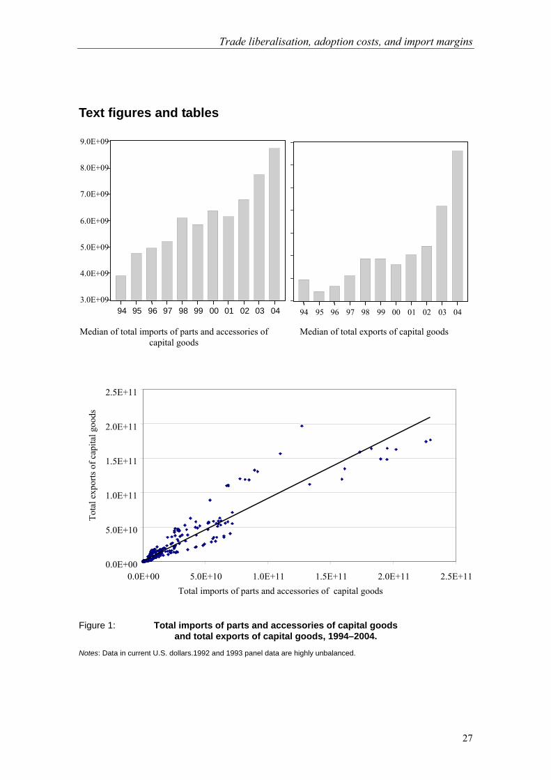
Trade liberalisation, adoption costs, and import margins
27
3.0E+09
4.0E+09
5.0E+09
6.0E+09
7.0E+09
8.0E+09
9.0E+09
94 95 96 97 98 99 00 01 02 03 04
94 95 96 97 98 99 00 01 02 03 04
Text figures and tables
Median of total imports of parts and accessories of
capital goods Median of total exports of capital goods
Figure 1: Total imports of parts and accessories of capital goods and total exports of capital goods, 1994–2004.
Notes: Data in current U.S. dollars.1992 and 1993 panel data are highly unbalanced.
0.0E+00
5.0E+10
1.0E+11
1.5E+11
2.0E+11
2.5E+11
0.0E+00 5.0E+10 1.0E+11 1.5E+11 2.0E+11 2.5E+11Total imports of parts and accessories of capital goods
Tota
l exp
orts
of c
apita
l goo
ds
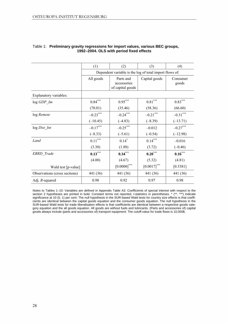
OSTEUROPA-INSTITUT REGENSBURG
28
Table 1: Preliminary gravity regressions for import values, various BEC groups, 1992–2004. OLS with period fixed effects
(1) (2) (3) (4) Dependent variable is the log of total import flows of:
All goods Parts and accessories
of capital goods
Capital goods
Consumer goods
Explanatory variables:
log GDP_Im
0.84*** (70.01)
0.95*** (35.46)
0.81*** (58.36)
0.83*** (66.60)
log Remote –0.23*** (–10.45)
–0.24*** (–4.83)
–0.21*** (–8.39)
–0.31*** (–13.71)
log Dist_Int
–0.17*** (–8.33)
–0.25*** (–5.61)
–0.012 (–0.54)
–0.27*** (–12.98)
Land 0.11*** (3.30)
0.14* (1.88)
0.14*** (3.72)
–0.016 (–0.46)
EBRD_Trade
Wald test [p-value]
0.13*** (4.00)
0.34*** (4.67)
[0.0000]***
0.20*** (5.32)
[0.0017]***
0.16*** (4.81)
[0.3381]
Observations (cross sections) 441 (36) 441 (36) 441 (36) 441 (36)
Adj. R-squared 0.98 0.92 0.97 0.98 Notes to Tables 1–10: Variables are defined in Appendix Table A3. Coefficients of special interest with respect to the section 2 hypotheses are printed in bold. Constant terms not reported, t-statistics in parentheses. * (**, ***) indicate significance at 10 (5, 1) per cent. The null hypothesis in the SUR-based Wald tests for country size effects is that coeffi-cients are identical between the capital goods equation and the consumer goods equation. The null hypothesis in the SUR-based Wald tests for trade liberalisation effects is that coefficients are identical between a respective goods cate-gory equation and the all goods equation. All goods are without fuels and lubricants. (Parts and accessories of) capital goods always include (parts and accessories of) transport equipment. The cutoff-value for trade flows is 10,000$.
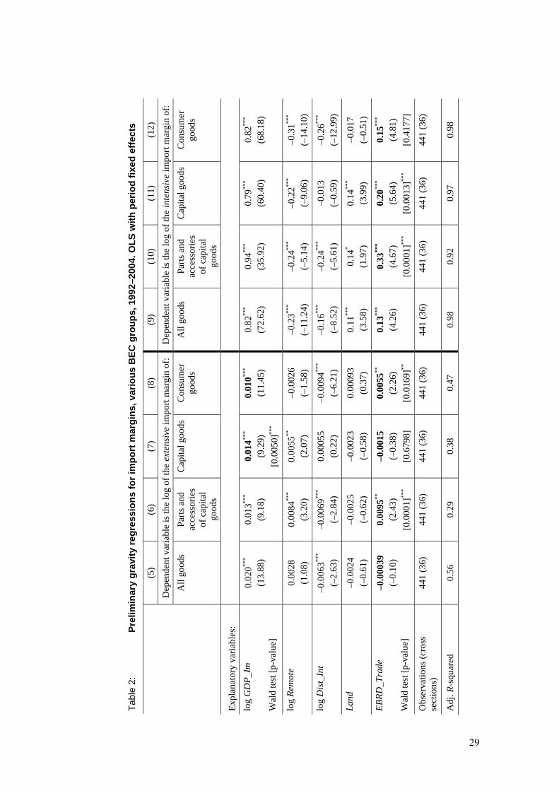
Tabl
e 2:
Pr
elim
inar
y gr
avity
regr
essi
ons
for i
mpo
rt m
argi
ns, v
ario
us B
EC g
roup
s, 1
992–
2004
. OLS
with
per
iod
fixed
effe
cts
(5)
(6)
(7)
(8)
(9)
(10)
(1
1)
(12)
D
epen
dent
var
iabl
e is
the
log
of th
e ex
tens
ive
impo
rt m
argi
n of
: D
epen
dent
var
iabl
e is
the
log
of th
e in
tens
ive
impo
rt m
argi
n of
:
All
good
s Pa
rts a
nd
acce
ssor
ies
of c
apita
l go
ods
Cap
ital g
oods
C
onsu
mer
go
ods
All
good
s Pa
rts a
nd
acce
ssor
ies
of c
apita
l go
ods
Cap
ital g
oods
C
onsu
mer
go
ods
Expl
anat
ory
varia
bles
:
log
GD
P_Im
W
ald
test
[p-v
alue
]
0.02
0***
(13.
88)
0.01
3***
(9.1
8)
0.01
4***
(9.2
9)
[0.0
050]
***
0.01
0***
(11.
45)
0.82
***
(72.
62)
0.94
***
(35.
92)
0.79
***
(60.
40)
0.82
***
(68.
18)
log
Rem
ote
0.00
28
(1.0
8)
0.00
84**
* (3
.20)
0.
0055
**
(2.0
7)
–0.0
026
(–1.
58)
–0.2
3***
(–11
.24)
–0
.24**
* (–
5.14
) –0
.22**
* (–
9.06
) –0
.31**
* (–
14.1
0)
log
Dis
t_In
t
–0.0
063**
* (–
2.63
) –0
.006
9***
(–2.
84)
0.00
055
(0.2
2)
–0.0
094**
* (–
6.21
) –0
.16**
* (–
8.52
) –0
.24**
* (–
5.61
) –0
.013
(–
0.59
) –0
.26**
* (–
12.9
9)
Land
–0
.002
4 (–
0.61
) –0
.002
5 (–
0.62
) –0
.002
3 (–
0.58
) 0.
0009
3 (0
.37)
0.
11**
* (3
.58)
0.
14*
(1.9
7)
0.14
***
(3.9
9)
–0.0
17
(–0.
51)
EBRD
_Tra
de
Wal
d te
st [p
-val
ue]
–0.0
0039
(–
0.10
) 0.
0095
**
(2.4
3)
[0.0
001]
***
–0.0
015
(–0.
38)
[0.6
798]
0.00
55**
(2
.26)
[0
.016
9]**
0.13
***
(4.2
6)
0.33
***
(4.6
7)
[0.0
001]
***
0.20
***
(5.6
4)
[0.0
013]
***
0.15
***
(4.8
1)
[0.4
177]
Obs
erva
tions
(cro
ss
sect
ions
) 44
1 (3
6)
441
(36)
44
1 (3
6)
441
(36)
44
1 (3
6)
441
(36)
44
1 (3
6)
441
(36)
Adj
. R-s
quar
ed
0.56
0.
29
0.38
0.
47
0.98
0.
92
0.97
0.
98
29

OSTEUROPA-INSTITUT REGENSBURG
30
Table 3: Gravity regressions for import values, various BEC groups, 1992–2004. OLS with period fixed effects
(13) (14) (15) (16) Dependent variable is the log of total import flows of:
All goods Parts and accessories of capital
goods
Capital goods
Consumer goods
Explanatory variables:
log GDP_Im
0.82*** (61.53)
0.89*** (30.27)
0.78*** (50.67)
0.82*** (58.22)
log Remote –0.24*** (–10.81)
–0.28*** (–5.78)
–0.23*** (–8.85)
–0.31*** (–13.52)
log Dist_Int
–0.15*** (–7.22)
–0.19*** (–4.09)
0.0098 (0.40)
–0.26*** (–11.95)
Land 0.12*** (3.72)
0.18** (2.48)
0.16*** (4.23)
–0.0017 (–0.05)
TradeLib
Wald test [p-value]
0.17*** (4.37)
0.57*** (6.58)
[0.0000]***
0.25*** (5.43)
[0.0054]***
0.15*** (3.51)
[0.5152]
Observations (cross sections) 442 (36) 442 (36) 442 (36) 442 (36)
Adj. R-squared 0.98 0.92 0.97 0.98
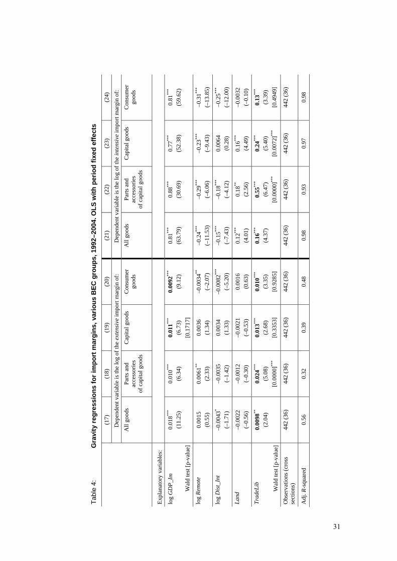
Tabl
e 4:
G
ravi
ty re
gres
sion
s fo
r im
port
mar
gins
, var
ious
BEC
gro
ups,
199
2–20
04. O
LS w
ith p
erio
d fix
ed e
ffect
s
(17)
(1
8)
(19)
(2
0)
(21)
(2
2)
(23)
(2
4)
Dep
ende
nt v
aria
ble
is th
e lo
g of
the
exte
nsiv
e im
port
mar
gin
of:
Dep
ende
nt v
aria
ble
is th
e lo
g of
the
inte
nsiv
e im
port
mar
gin
of:
All
good
s Pa
rts a
nd
acce
ssor
ies
of c
apita
l goo
ds
Cap
ital g
oods
Con
sum
er
good
s A
ll go
ods
Parts
and
ac
cess
orie
s of
cap
ital g
oods
Cap
ital g
oods
Con
sum
er
good
s
Expl
anat
ory
varia
bles
:
log
GD
P_Im
Wal
d te
st [p
-val
ue]
0.01
8***
(11.
25)
0.01
0***
(6.3
4)
0.01
1***
(6.7
3)
[0.1
717]
0.00
92**
* (9
.12)
0.
81**
* (6
3.79
) 0.
88**
* (3
0.69
) 0.
77**
* (5
2.38
) 0.
81**
* (5
9.62
)
log
Rem
ote
0.00
15
(0.5
5)
0.00
61**
(2
.33)
0.
0036
(1
.34)
–0
.003
4**
(–2.
07)
–0.2
4***
(–11
.53)
–0
.29**
* (–
6.06
) –0
.23**
* (–
9.43
) –0
.31**
* (–
13.8
5)
log
Dis
t_In
t
–0.0
043*
(–1.
71)
–0.0
035
(–1.
42)
0.00
34
(1.3
3)
–0.0
082**
* (–
5.20
) –0
.15**
* (–
7.43
) –0
.18**
* (–
4.12
) 0.
0064
(0
.28)
–0
.25**
* (–
12.0
0)
Land
–0
.002
2 (–
0.56
) –0
.001
2 (–
0.30
) –0
.002
1 (–
0.53
) 0.
0016
(0
.63)
0.
12**
* (4
.01)
0.
18**
(2
.56)
0.
16**
* (4
.49)
–0
.003
2 (–
0.10
)
Trad
eLib
Wal
d te
st [p
-val
ue]
0.00
98**
(2
.04)
0.
024**
* (5
.08)
[0
.000
0]**
*
0.01
3***
(2.6
8)
[0.3
353]
0.01
0***
(3.3
5)
[0.9
285]
0.16
***
(4.3
7)
0.55
***
(6.4
7)
[0.0
000]
***
0.24
***
(5.4
0)
[0.0
072]
***
0.13
***
(3.3
9)
[0.4
949]
Obs
erva
tions
(cro
ss
sect
ions
) 44
2 (3
6)
442
(36)
44
2 (3
6)
442
(36)
44
2 (3
6)
442
(36)
44
2 (3
6)
442
(36)
Adj
. R-s
quar
ed
0.56
0.
32
0.39
0.
48
0.98
0.
93
0.97
0.
98
31

OSTEUROPA-INSTITUT REGENSBURG
32
Table 5: Gravity regressions for import values, various BEC groups, 1992–2001. OLS with period fixed effects
(25) (26) (27) (28) Dependent variable is the log of total import flows of:
All goods Parts and accessories of capital
goods
Capital goods
Consumer goods
Explanatory variables:
log GDP_Im
0.83*** (55.53)
0.90*** (26.46)
0.80*** (46.28)
0.80*** (49.18)
log Remote –0.24*** (–9.66)
–0.27*** (–4.92)
–0.21*** (–7.52)
–0.33*** (–12.60)
log Dist_Int
–0.17*** (–7.41)
–0.21*** (–3.92)
–0.014 (–0.54)
–0.25*** (–9.85)
Land 0.11*** (2.98)
0.17* (1.97)
0.17*** (3.97)
0.042 (1.02)
Lora_ext
Wald test [p-value]
0.26*** (3.27)
0.81*** (4.40)
[0.0000]***
0.39*** (4.18)
[0.0279]**
0.46*** (5.32)
[0.0216]**
Observations (cross sections) 329 (35) 329 (35) 329 (35) 329 (35)
Adj. R-squared 0.98 0.92 0.97 0.98

Tabl
e 6:
G
ravi
ty re
gres
sion
s fo
r im
port
mar
gins
, var
ious
BEC
gro
ups,
1992
–200
1. O
LS w
ith p
erio
d fix
ed e
ffect
s
(29)
(3
0)
(31)
(3
2)
(33)
(3
4)
(35)
(3
6)
Dep
ende
nt v
aria
ble
is th
e lo
g of
the
exte
nsiv
e im
port
mar
gin
of:
Dep
ende
nt v
aria
ble
is th
e lo
g of
the
inte
nsiv
e im
port
mar
gin
of:
All
good
s Pa
rts a
nd
acce
ssor
ies
of c
apita
l goo
ds
Cap
ital g
oods
Con
sum
er
good
s A
ll go
ods
Parts
and
ac
cess
orie
s of
cap
ital g
oods
Cap
ital g
oods
Con
sum
er
good
s
Expl
anat
ory
varia
bles
:
log
GD
P_Im
W
ald
test
[p-v
alue
]
0.02
0***
(10.
12)
0.01
3***
(6.2
8)
0.01
3***
(6.6
9)
[0.0
203]
0.00
96**
* (7
.91)
0.
81**
* (5
7.72
) 0.
89**
* (2
6.84
) 0.
78**
* (4
7.90
) 0.
79**
* (5
0.38
)
log
Rem
ote
0.00
19
(0.5
9)
0.00
80**
(2
.45)
0.
0056
* (1
.75)
–0
.003
5* (–
1.76
) –0
.24**
* (–
10.3
7)
–0.2
8***
(–5.
21)
–0.2
2***
(–8.
13)
–0.3
3***
(–12
.93)
log
Dis
t_In
t
–0.0
063**
(–
2.09
) –0
.005
6* (–
1.82
) 0.
0006
1 (0
.20)
–0
.008
2***
(–4.
33)
–0.1
7***
(–7.
60)
–0.2
0***
(–3.
93)
–0.0
15
(–0.
60)
–0.2
4***
(–9.
88)
Land
–0
.002
0 (–
0.40
) 0.
0018
(0
.36)
0.
0010
(0
.20)
0.
0037
(1
.19)
0.
12**
* (3
.23)
0.
17**
(2
.00)
0.
17**
* (4
.16)
0.
039
(0.9
7)
Lora
_ext
Wal
d te
st [p
-val
ue]
0.01
3 (1
.22)
0.
030**
* (2
.79)
[0
.014
4]**
0.02
4**
(2.2
3)
[0.1
209]
0.02
3***
(3.5
2)
[0.1
065]
0.25
***
(3.3
1)
0.78
***
(4.3
6)
[0.0
000]
***
0.36
***
(4.1
3)
[0.0
429]
**
0.44
***
(5.2
4)
[0.0
244]
**
Obs
erva
tions
(cro
ss
sect
ions
) 32
9 (3
5)
329
(35)
32
9 (3
5)
329
(35)
32
9 (3
5)
329
(35)
32
9 (3
5)
329
(35)
Adj
. R-s
quar
ed
0.56
0.
29
0.40
0.
49
0.98
0.
92
0.98
0.
98
33

Tabl
e 7:
G
ravi
ty re
gres
sion
s fo
r im
port
mar
gins
(nat
iona
l pro
duct
diff
eren
tiatio
n), v
ario
us B
EC g
roup
s,
19
92–2
004.
OLS
with
per
iod
fixed
effe
cts
(37)
(3
8)
(39)
(4
0)
(41)
(4
2)
(43)
(4
4)
Dep
ende
nt v
aria
ble
is th
e lo
g of
the
exte
nsiv
e im
port
mar
gin
of:
Dep
ende
nt v
aria
ble
is th
e lo
g of
the
inte
nsiv
e im
port
mar
gin
of:
All
good
s Pa
rts a
nd
acce
ssor
ies
of c
apita
l goo
ds
Cap
ital g
oods
Con
sum
er
good
s A
ll go
ods
Parts
and
ac
cess
orie
s of
cap
ital g
oods
Cap
ital g
oods
Con
sum
er
good
s
Expl
anat
ory
varia
bles
:
log
GD
P_Im
Wal
d te
st [p
-val
ue]
0.27
***
(25.
74)
0.26
***
(20.
40)
0.25
***
(22.
35)
[0.3
341]
0.24
***
(21.
00)
0.55
***
(44.
07)
0.63
***
(23.
71)
0.54
***
(45.
44)
0.58
***
(45.
17)
log
Rem
ote
0.00
19
(0.1
1)
0.00
64
(0.3
0)
0.01
9 (1
.04)
–0
.053
***
(–2.
83)
–0.2
4***
(–11
.65)
–0
.29**
* (–
6.57
) –0
.25**
* (–
12.5
9)
–0.2
6***
(–12
.31)
log
Dis
t_In
t
–0.0
76**
* (–
4.61
) –0
.025
(–
1.26
) –0
.029
* (–
1.69
) –0
.11**
* (–
6.23
) –0
.075
***
(–3.
83)
–0.1
6***
(–3.
94)
0.03
9**
(2.1
2)
–0.1
5***
(–7.
57)
Land
0.
13**
* (4
.82)
0.
18**
* (5
.72)
0.
15**
* (5
.39)
0.
068**
(2
.42)
–0
.003
0 (–
0.10
) –0
.001
7 (–
0.03
) 0.
014
(0.4
8)
–0.0
69**
(–
2.20
)
Trad
eLib
Wal
d te
st [p
-val
ue]
0.05
3* (1
.70)
0.
12**
* (3
.09)
[0
.000
0]**
*
0.05
6* (1
.71)
[0
.706
5]
0.17
***
(5.0
8)
[0.0
000]
***
0.12
***
(3.2
4)
0.45
***
(5.8
1)
[0.0
000]
***
0.19
***
(5.5
1)
[0.0
033]
***
–0.0
25
(–0.
66)
[0.0
000]
***
Obs
erva
tions
(cro
ss
sect
ions
) 44
2 (3
6)
442
(36)
44
2 (3
6)
442
(36)
44
2 (3
6)
442
(36)
44
2 (3
6)
442
(36)
Adj
. R-s
quar
ed
0.86
0.
82
0.84
0.
83
0.96
0.
89
0.97
0.
96
34

Tabl
e 8:
G
ravi
ty re
gres
sion
s fo
r im
port
mar
gins
, var
ious
BEC
gro
ups,
199
2–20
04.
O
LS w
ith c
ross
-sec
tion
and
perio
d fix
ed e
ffect
s
(45)
(4
6)
(47)
(4
8)
(49)
(5
0)
(51)
(5
2)
Dep
ende
nt v
aria
ble
is th
e lo
g of
the
exte
nsiv
e im
port
mar
gin
of:
Dep
ende
nt v
aria
ble
is th
e lo
g of
the
inte
nsiv
e im
port
mar
gin
of:
All
good
s Pa
rts a
nd
acce
ssor
ies
of c
apita
l goo
ds
Cap
ital g
oods
Con
sum
er
good
s A
ll go
ods
Parts
and
ac
cess
orie
s of
cap
ital g
oods
Cap
ital g
oods
Con
sum
er
good
s
Expl
anat
ory
varia
bles
:
log
GD
P_Im
Wal
d te
st [p
-val
ue]
0.04
0***
(7.1
4)
0.03
4***
(4.7
2)
0.03
3***
(3.6
9)
[0.7
902]
0.03
1***
(7.4
3)
0.80
***
(15.
05)
0.88
***
(10.
20)
0.93
***
(12.
87)
0.86
***
(14.
65)
Trad
eLib
Wal
d te
st [p
-val
ue]
0.01
2***
(4.1
7)
0.02
2***
(6.2
7)
[0.0
010]
***
0.02
5***
(5.6
7)
[0.0
002]
***
0.00
52**
(2
.57)
[0
.001
9]**
*
0.14
***
(5.2
1)
0.23
***
(5.5
2)
[0.0
002]
***
0.10
***
(2.8
1)
[0.1
065]
0.04
3 (1
.49)
[0
.000
0]**
*
Obs
erva
tions
(cro
ss
sect
ions
) 44
2 (3
6)
442
(36)
44
2 (3
6)
442
(36)
44
2 (3
6)
442
(36)
44
2 (3
6)
442
(36)
Adj
. R-s
quar
ed
0.93
0.
82
0.76
0.
89
0.99
0.
99
0.99
0.
99
35

Tabl
e 9:
G
ravi
ty re
gres
sion
s fo
r im
port
mar
gins
(nat
iona
l pro
duct
diff
eren
tiatio
n), v
ario
us B
EC g
roup
s,
19
92–2
004.
OLS
with
cro
ss-s
ectio
n an
d pe
riod
fixed
effe
cts
(53)
(5
4)
(55)
(5
6)
(57)
(5
8)
(59)
(6
0)
Dep
ende
nt v
aria
ble
is th
e lo
g of
the
exte
nsiv
e im
port
mar
gin
of:
Dep
ende
nt v
aria
ble
is th
e lo
g of
the
inte
nsiv
e im
port
mar
gin
of:
All
good
s Pa
rts a
nd
acce
ssor
ies
of c
apita
l goo
ds
Cap
ital g
oods
C
onsu
mer
go
ods
All
good
s Pa
rts a
nd
acce
ssor
ies
of c
apita
l goo
ds
Cap
ital g
oods
C
onsu
mer
go
ods
Expl
anat
ory
varia
bles
:
log
GD
P_Im
Wal
d te
st [p
-val
ue]
0.35
***
(11.
12)
0.36
***
(10.
21)
0.40
***
(10.
58)
[0.4
240]
0.42
***
(11.
40)
0.49
***
(10.
92)
0.55
***
(6.8
8)
0.56
***
(9.3
6)
0.47
***
(9.2
9)
Trad
eLib
Wal
d te
st [p
-val
ue]
0.10
***
(6.5
4)
0.14
***
(8.0
4)
[0.0
000]
***
0.11
***
(6.1
2)
[0.0
448]
**
0.04
8***
(2.6
3)
[0.0
000]
***
0.04
6**
(2.0
8)
0.12
***
(2.9
5)
[0.0
046]
***
0.01
1 (0
.36)
[0
.075
9]*
0.00
066
(0.0
3)
[0.0
060]
***
Obs
erva
tions
(cro
ss se
ctio
ns)
442
(36)
44
2 (3
6)
442
(36)
44
2 (3
6)
442
(36)
44
2 (3
6)
442
(36)
44
2 (3
6)
Adj
. R-s
quar
ed
0.98
0.
98
0.98
0.
98
0.99
0.
99
0.99
0.
99
36
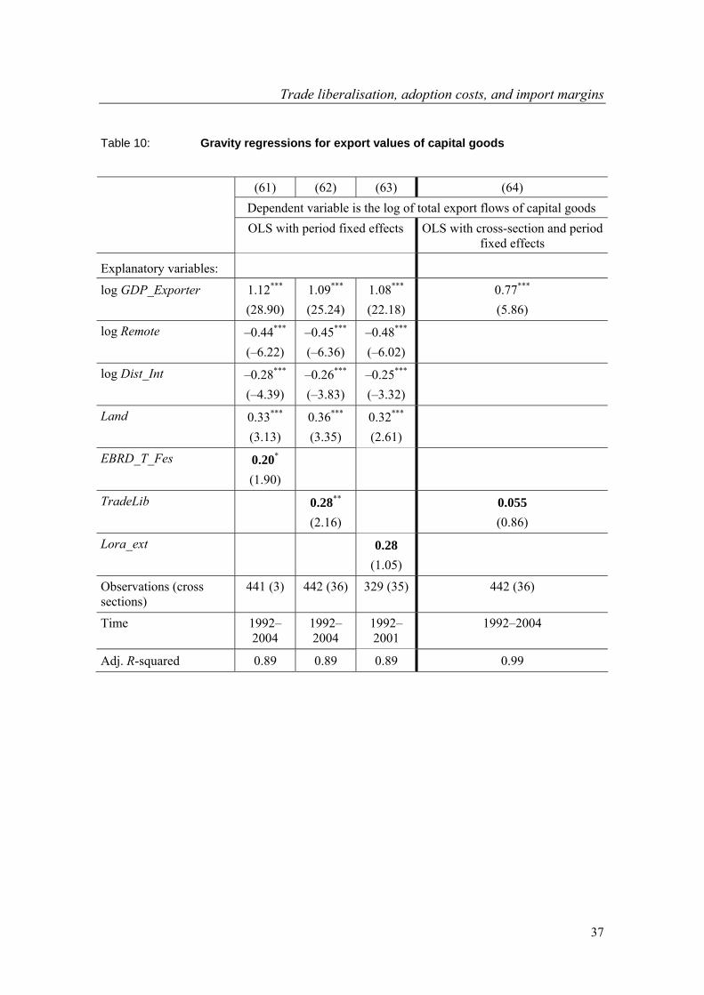
Trade liberalisation, adoption costs, and import margins
37
Table 10: Gravity regressions for export values of capital goods
(61) (62) (63) (64)
Dependent variable is the log of total export flows of capital goods
OLS with period fixed effects OLS with cross-section and period fixed effects
Explanatory variables:
log GDP_Exporter
1.12*** (28.90)
1.09*** (25.24)
1.08*** (22.18)
0.77*** (5.86)
log Remote –0.44*** (–6.22)
–0.45*** (–6.36)
–0.48*** (–6.02)
log Dist_Int
–0.28*** (–4.39)
–0.26*** (–3.83)
–0.25*** (–3.32)
Land 0.33*** (3.13)
0.36*** (3.35)
0.32*** (2.61)
EBRD_T_Fes 0.20* (1.90)
TradeLib 0.28** (2.16)
0.055 (0.86)
Lora_ext 0.28 (1.05)
Observations (cross sections)
441 (3) 442 (36) 329 (35) 442 (36)
Time 1992–2004
1992–2004
1992–2001
1992–2004
Adj. R-squared 0.89 0.89 0.89 0.99

OSTEUROPA-INSTITUT REGENSBURG
38
Appendix: Commodity classifications, country and time coverage
A.1 Commodity classifications
SITC The Standard International Trade Classification, Revision 3 (SITC, Rev.3) was used at all aggregation levels (1-, 2- and 3-digit levels for checking totals, 4- and 5-digit levels for counting SITC categories).
There are 3,121 basic headings or basic categories in the SITC, Rev.3, 2,824 at the 5-digit level and 297 at 4-digits, that are not disaggregated any further. The 3-digit group 334 (petroleum products), which is divided into eight final headings in SITC, Rev.3, is in fact not subdivided by many reporting countries, so I treat it as a single heading. This leaves 3,114 basic categories, as the level of aggregation of the SITC, Rev.3 to work with. BEC The United Nations Statistics Division’s Classification by BEC (Broad Economic Cate-gories, available online at http://unstats.un.org/unsd/cr/family2.asp?Cl=10) allows for headings of the SITC, Rev.3 to be grouped into 19 activities covering primary and proc-essed foods and beverages, industrial supplies, fuels and lubricants, capital goods and transport equipment, and consumer goods according to their durability. The BEC also provides for the rearrangement of these 19 activities (on the basis of SITC categories’ main end-use) to approximate the basic System of National Accounts (SNA) activities, namely, primary goods, intermediate goods, capital goods, and consumer goods.
– Table A1 about here – Primary goods (BEC headings 111, 21) consist of 272 SITC, Rev.3 categories and
include primary food and beverages designated mainly for industrial use and primary industrial supplies (raw materials).
Intermediate goods (BEC headings 121, 22, 42, 53) consist of 1,627 SITC, Rev.3 categories and include: processed food and beverages designated mainly for industry; processed industrial supplies; parts and accessories of capital goods and transport equipment.
Capital goods (BEC headings 41, 521) comprise 471 categories at the 4- and 5-digit levels of the SITC, Rev.3 and include: machinery such as electric generators and com-puters; industrial transport equipment such as finished ships, road vehicles, aircraft, railway and tramway rolling stock; other manufactured goods such as medical furniture, which are used by industry, government and non-profit private institutions.
Consumer goods (BEC headings 112, 122, 522, 6) cover 704 categories at 4- and 5-digits of the SITC and include primary and processed food and beverages designated mainly for household consumption; non-industrial transport equipment, such as motor-cycles and bicycles; other consumer goods.

Trade liberalisation, adoption costs, and import margins
39
SITC categories falling under BEC headings 51, 3, and 7 are excluded from our rear-rangement into primary, intermediate, capital, and consumer goods for various reasons. ‘Motor vehicles for the transport of passengers’, SITC, Rev.3, heading 7812 (equivalent to BEC heading 51), cannot be divided into capital or consumer goods. Similar reason-ing holds for motor spirits. By definition, intermediate goods should also include pri-mary and processed fuels and lubricants other than motor spirit, but in this data set ‘fu-els and lubricants’, which include 32 4- and 5-digit headings of the SITC, Rev.3, are not used, in part due to countries’ incomparable reporting practices (see above). BEC 7, ‘goods not elsewhere classified’, comprises 14 basic headings of the SITC, namely, military equipment, including arms and ammunitions, special transactions, postal pack-ages, etc., which are all excluded. A.2 Country and period coverage
Reporting countries’ data were extracted for 36 countries from Europe and North Amer-ica. Belgium and Luxembourg are treated as one country throughout as reported until 1998. The data cover 1992–2004 but not all countries report in each year (average: 34.1 countries per year).
– Table A2 about here – Partner countries comprise the rest of the world (for total imports), and 55 individual
countries (i.e., the 36 reporter-countries plus: Bosnia and Herzegovina, 12 CIS econo-mies (Armenia, Azerbaijan, Belarus, Georgia, Kazakhstan, Kyrgyzstan, Moldova, Rus-sia, Turkmenistan, Ukraine, Tajikistan, Uzbekistan) and six Asian economies (China, Hong Kong, Japan, South Korea, Taiwan, and Thailand) for imports and thus for the extensive margin count in the expanded product space allowing for product differentia-tion by country of origin. These partner countries generally account for 80–95 per cent of reported imports, although Canada and the United States trade extensively with south American countries that are not included among the 55 partners. Also, the Czech Re-public, Slovakia and Macedonia are available as partner countries only from 1993 on.
– Table A3 about here –
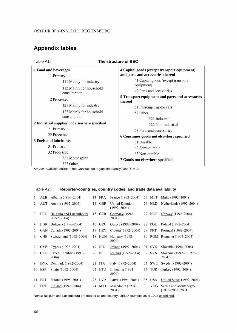
OSTEUROPA-INSTITUT REGENSBURG
40
Appendix tables
Table A1: The structure of BEC
1 Food and beverages 11 Primary
111 Mainly for industry
112 Mainly for household consumption
12 Processed 121 Mainly for industry
122 Mainly for household consumption
2 Industrial supplies not elsewhere specified 21 Primary 22 Processed
3 Fuels and lubricants 31 Primary 32 Processed
321 Motor spirit 322 Other
4 Capital goods (except transport equipment) and parts and accessories thereof
41 Capital goods (except transport equipment) 42 Parts and accessories
5 Transport equipment and parts and accessories thereof
51 Passenger motor cars 52 Other
521 Industrial 522 Non-industrial
53 Parts and accessories 6 Consumer goods not elsewhere specified
61 Durable 62 Semi-durable 63 Non-durable
7 Goods not elsewhere specified
Source: Available online at http://unstats.un.org/unsd/cr/family2.asp?Cl=10
Table A2: Reporter-countries, country codes, and trade data availability
1 ALB Albania (1996–2004) 13 FRA France (1992–2004) 25 MLT Malta (1992–2004)
2 AUT Austria (1992–2004) 14 GBR United Kingdom (1992–2004)
26 NLD Netherlands (1992–2004)
3 BEL Belgium and Luxembourg (1992–2004)
15 GER Germany (1992–2004)
27 NOR Norway (1992–2004)
4 BGR Bulgaria (1996–2004) 16 GRC Greece (1992–2004) 28 POL Poland (1992–2004)
5 CAN Canada (1992–2004) 17 HRV Croatia (1992–2004) 29 PRT Portugal (1992–2004)
6 CHE Switzerland (1992–2004) 18 HUN Hungary (1992–2004)
30 ROM Romania (1994–2004)
7 CYP Cyprus (1992–2004) 19 IRL Ireland (1992–2004) 31 SVK Slovakia (1994–2004)
8 CZE Czech Republic (1993–2004)
20 ISL Iceland (1992–2004) 32 SVN Slovenia (1992–3, 1995–2004))
9 DNK Denmark (1992–2004) 21 ITA Italy (1992–2004) 33 SWE Sweden (1992–2004)
10 ESP Spain (1992–2004) 22 LTU Lithuania (1994–2004)
34 TUR Turkey (1992–2004)
11 EST Estonia (1995–2004) 23 LVA Latvia (1994–2004) 35 USA United States (1992–2004)
12 FIN Finland (1992–2004) 24 MKD Macedonia (1994–2004)
36 YUG Serbia and Montenegro (1996–2002, 2004)
Notes: Belgium and Luxembourg are treated as one country. OECD countries as of 1992 underlined.

Trade liberalisation, adoption costs, and import margins
41
Table A3: Variables used in regressions (1)–(64) in Tables 1–10
Variable Definition Source Notes
Dependent variables
IMPORTSc,t Imports of country c at time t from ROW in current dollars
UN COMTRADE See Appendix.
EMc,t and IMc,t
Extensive and intensive margins of imports over the SITC Rev.3 product space
Own computations on the basis of UN COMTRADE
Defined by 3,114 SITC Rev.3 categories; see Text and Appendix.
EMc,t(PD) and IMc,t(PD)
Extensive and intensive margins of imports over an expanded product space allowing for product differen-tiation by country of origin
Own computations on the basis of UN COMTRADE
Defined by 168,156 pro-ducts, i.e., by 3,114 SITC Rev.3 categories times 54 respective source countries; see Text and Appendix.
Explanatory variables
GDP_Imc,t Import country GDP in current dollars
World Development Indicators 2007
Remotec Average distance by air to the closest core economic area
Gallup and Sachs (1999)
Smallest distance of a country’s capital to one of the following three cities: New York, Rotterdam, or Tokyo
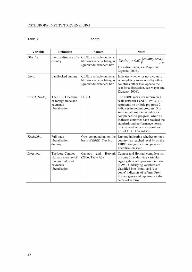
OSTEUROPA-INSTITUT REGENSBURG
42
Table A3 contd.:
Variable Definition Source Notes
Dist_Intc Internal distance of a country
CEPII, available online at http://www.cepii.fr/anglaisgraph/bdd/distances.htm
πareacountry
cDistInt 67.0=
For a discussion, see Mayer and Zignano (2006).
Landc Landlocked dummy CEPII, available online at http://www.cepii.fr/anglaisgraph/bdd/distances.htm
Indicates whether or not a country is completely surrounded by other countries rather than open to the sea; for a discussion, see Mayer and Zignano (2006).
EBRD_Tradec,t The EBRD measure of foreign trade and payments liberalisation
EBRD The EBRD measures reform on a scale between 1 and 4+ (=4.33); 1 represents no or little progress; 2 indicates important progress; 3 is substantial progress; 4 indicates comprehensive progress, while 4+ indicates countries have reached the standards and performance norms of advanced industrial coun-tries, i.e., of OECD coun-tries.
TradeLibc,t Full trade liberalisation dummy
Own computations on the basis of EBRD_Tradec,t
Dummy indicating whether or not a country has reached level 4+ on the EBRD foreign trade and payments liberalisation scale.
Lora_extc,t The Lora-Campos-Horvath measure of foreign trade and payments liberalisation
Campos and Horvath (2006, Table A3)
Campos and Horvath compile a list of some 30 underlying variables. Aggregation is as proposed in Lora (1998). Underlying variables are classified into ‘input’ and ‘out-come’ indicators of reform. From this are generated input-only indi-cators of reform.