trade liberalization and disaggregated import demand in...

Modern Economy, 2015, 6, 316-337 Published Online March 2015 in SciRes. http://www.scirp.org/journal/me http://dx.doi.org/10.4236/me.2015.63030

How to cite this paper: Samuel, G.M. (2015) Trade Liberalization and Disaggregated Import Demand in Uganda. Modern Economy, 6, 316-337. http://dx.doi.org/10.4236/me.2015.63030

Trade Liberalization and Disaggregated Import Demand in Uganda Gaalya Micah Samuel Research and Planning Division, Commissioner General’s Office, Uganda Revenue Authority, Kampala, Uganda Email: [email protected] Received 21 February 2015; accepted 7 March 2015; published 10 March 2015

Copyright © 2015 by author and Scientific Research Publishing Inc. This work is licensed under the Creative Commons Attribution International License (CC BY). http://creativecommons.org/licenses/by/4.0/

Abstract Studies investigating determinants of import demand for Uganda present aggregate findings yet there is a need to disaggregate the findings for specific sectors. This creates a research gap on dis-aggregated findings of import demand. This research attempts to fill this research gap by estab-lishing determinants of import demand using disaggregated sector level data for consumer, in-termediate and capital goods. The study estimates the long-run and short-run import demand elasticities for consumer, intermediate and capital goods over the period (1994 to 2012). The re-sults show that there exists a cointegrating relationship between the disaggregated import de-mand and the following set of variables; relative import price, GDP per capita, real effective ex-change rate, foreign exchange rate reserves and trade openness. The long run elasticity appears more responsive to import demand compared to the short-run elasticity. Importantly the effect of a change in trade openness on the volume of imports is positive, suggesting trade liberalization increases import demand.

Keywords Trade Liberalization, Import Demand, Consumer Goods, Intermediate Goods, Capital Goods, Uganda

1. Introduction Trade reforms have been a major economic feature of the world trade system for the latter part of the twentieth century. Trade reforms have seen a substantial expansion in trade flows, capital movements, information and technology as well as mobility of labour across borders. These have led to an increase in world production and consequently an improvement in world economic welfare. During the period physical distances have become less significant, cultural differences have been reduced, consumption patterns as well as tastes and preferences

http://www.scirp.org/journal/me

http://dx.doi.org/10.4236/me.2015.63030

http://dx.doi.org/10.4236/me.2015.63030

http://www.scirp.org

mailto:[email protected]

http://creativecommons.org/licenses/by/4.0/

G. M. Samuel

317

have begun converging. Accordingly, the world economy has grown closer as trade regimes are modified and trade barriers reduced.

Trade reform is associated with the reduction, removal and elimination of tariff and other trade barriers such as quotas on imports, subsidies and nontariff barriers. It also includes the removal of trade-distorting policies, free access to market information, reduction of monopoly or oligopoly power, free movement of capital and la-bour between and within countries and the creation of free trade zones. Trade liberalization may also take other forms such as free trade area, trade blocs and free trade agreements e.g. bilateral, multilateral or regional [1].

Theoretically the influence of trade liberalization on imports is considered to be an indirect outcome derived from the response of consumption and production decisions to price changes, with price changes triggered by trade reforms [2]. There are two conflicting issues concerning imports in developing countries. First, for balance of payments reasons it may be necessary to restrict imports. A deterioration in balance of payment and terms of trade makes it necessary for developing countries to restrict imports. Second, the restriction of imports does not only cause import revenue and overall revenues to fall but can also lead to an exacerbation of inflationary ten-dencies in the domestic economy. In some cases, some of the policies designed to restrict imports or increase revenue may have the opposite effect. Import demand stability is, in fact, a prerequisite for an effective trade policy [3]. In other words, effective trade policy formulation requires that the change in import demand does not change significantly over time.

Imports are a key part of international trade and the import of consumer, intermediate and capital goods are vital to economic growth. Imported goods directly affect investment which, in turn, constitutes the engine of economic growth. In Uganda, examples of imported goods include medicaments, heavy machinery and equip-ment and other raw materials, such as crude oil.

The performance of import shows that initially, most developing countries could place orders with suppliers for any quantity or value of imports. However by the early 1970’s, most developing countries began experienc-ing chronic foreign exchange problems, which represented a looming economic crisis [4]. This showed that in the previous decades, the capacity to import for some developing countries, including Uganda, had declined or stagnated while import demand continued to grow. In the 1980’s and early 1990’s, the IMF recommended a number of economic recovery programmes for developing countries as a way of averting the economic crisis. As in most African economies, Uganda implemented structural adjustment programmes (SAPs) in the late 1980’s, of which trade liberalization and tax policy reform was a component. Before the inception of the economic crisis, Uganda’s exports and imports grew at almost an equal rate, with exports nearly matching imports in value [4]. The inception of the reforms in 1987 saw faster growth in imports, as shown in (Figure 1), to date Uganda’s negative trade balance continues to rise. In addition imports and exports take a similar trend suggesting a corre-lation between imports and exports.

In Uganda increased import demand has caused a recurrent balance of payment disequilibrium [5]. For exam-ple in the period 2001-2012, while world average imports growth in value was 7.7 percent, Uganda’s average imports growth was 13.4 percent, Uganda’s average imports growth almost doubled the world import growth1. The import growth appears to have been influenced by Uganda’s trade liberalization preferences that have dom-inated by tariff liberalization. Import growth has seen a rise in the importation of all categories of import goods. For example the construction industry has played a key part in the growth of imports, this is reflected in the wide range of construction related imports, especially construction equipment, cement and fittings for residential and commercial structures.

An analysis of the structure of imports shows that Uganda mostly imports consumer, intermediate and capital goods. The top 10 items imported in 2001-2012 at HSC six-digit level, according to share in value were; Other petroleum oils and preparations (14.5%), petroleum oils and preparations (7.16%), commodities not elsewhere specified (3.9%), medicaments in dosage (3.18%), Telephones for cellular networks mobile telephones (2.86%), Automobiles reciproca piston engine displace > 1500 cc to 3000 cc (2.73%), Palm oil and its fractions refined but not chemically modified (2.1%), Refined sugar in solid form (2.06%), Palm oil, crude (1.69%), Graders and levellers, self-propelled (1.17%). These together account for 47.4 percent of Uganda’s imports for the period2. The top ten share in value in Uganda’s imports for the period 2001-2012 in percentages were from the following countries; India (20.9%), China (11.3%), Kenya (9.8%), UAE (7.5%); Japan (5.4%), South Africa (4.9%), Saudi Arabia (4.9%), Indonesia (3.9%), Germany (2.1%) and the UK (2.1%). These together account for 74.4 percent

1Author’s computation based on the COMTRADE and TRAINS data, July 2013. 2Author’s computation based on the COMTRADE and TRAINS data, July 2013.

G. M. Samuel

318

Figure 1. Uganda’s exports and imports, percentage of GDP. Source: Author’s computation based on the COMTRADE and TRAINS data, July 2012.

of Uganda’s imports for the period. However, in spite of the predominance of imports from the top ten countries, there are a number of other exporters to Uganda.

Problem Statement As in most African economies, Uganda implemented structural adjustment programmes (SAPs) in the late 1980’s and early 1990’s. The programmes and policy measures sought to reduce external disequilibrium while strengthening production capacity. Among the principal measures to bring about external balance, the policies attempted to influence imports and tax policy. Prior and during the reform period, Uganda became more preoc-cupied with mobilizing external financial assistance, thereby incurring debt. The debt burden, however, has caused a decrease in public investment spending and an increase in budgetary deficits. Uganda has also under-taken substantial trade liberalization in an effort to improve its balance of payment situation [5]. This has neces-sitated knowledge of the determinants of import demand. It has also become necessary to determine whether the pattern of import demand has changed due to these policy changes.

Although studies on Uganda’s import demand exist, for example [6]-[8], these studies provide aggregate findings, despite the need to disaggregate results for specific sectors. This is a methodological weakness which gives biased results, given the compositions of aggregate imports. As a result, there appears to be a gap on dis-aggregated import demand findings for Uganda. This study contributes to trade literature by undertaking a study that solve this methodological weakness by investigating the responsiveness of disaggregated import elasticities for consumer, intermediate and capital goods import demand for Uganda.

2. Uganda’s Import Policies Uganda has used several trade policy measures towards strengthening the competitiveness of the domestic economy [1]. The policy measures are intended to address Uganda’s uncompetitive trade regime. The trade re-gime was characterized with very high import tariffs and inefficient customs system, bureaucratic import li-censing system that acted as a barrier to international trade, statutory exemptions from import taxes to some business entities and organizations like diplomatic bodies, embassies and government agencies and several non-tariff barriers to trade including quantitative restrictions and import bans [1]. The above features made it inevitable for Uganda to undertake trade policy reforms given that the economy would have remained uncompe-titive.

The key hallmark of the trade reform process has been reduction and harmonization of tariffs, removal of quantitative trade barriers and acceding to trade liberalizing agreements such as the EAC trade agreement in 2001, COMESA in 1985, WTO in 1995 and others bilateral and unilateral liberalization arrangements. Other features of the trade liberalization processes include unilateral tariffs cut, import licensing system reforms, and extensive removal of non-tariff barriers.

0

5

10

15

20

25

30

35

40

1982

1983

1984

1985

1986

1987

1988

1989

1990

1991

1992

1993

1994

1995

1996

1997

1998

1999

2000

2001

2002

2003

2004

2005

2006

2007

2008

2009

2010

2011

2012

% o

f GD

P

Years

Exports (% of GDP) Imports (% of GDP)

G. M. Samuel

319

Particularly under the EAC liberalization arrangement the very first liberalization policy was the formation of the Customs Union between Kenya and Uganda in 1917. Later in 1927, the then Tanganyika (Tanzania main-land) joined the Customs Union. The second major stage in the trade liberalization was the first East African Community that lasted between 1967 and 1977. The third major stage is the current EAC trade agreement that was formed in 1999, following ratification of the EAC treaty by the initial partner states of the Republic of Kenya, the United Republic of Tanzania and the Republic of Uganda. In 2007 Burundi and Rwanda joined the EAC as full members. Some potential candidates of the EAC are Malawi, Democratic Republic of Congo, Zam-bia, Southern Sudan and Sudan. On 1st July 2012, the five members East African Community became a single market and preparations are under way for it to achieve a full monetary union and a possible political federation.

In addition to the EAC regional trade agreement, Uganda has been a GATT contracting party since indepen-dence in 1962 and it acceded to the WTO agreement in 1995. The WTO is a successor to the GATT. Uganda has implemented various measures in compliance with its commitments to the GATT and WTO commitments. Some of the measurers include; restructuring of the tariff system, review of the trade laws in accordance with the Trade Related Aspects of Intellectual Property Rights (TRIPs) agreement and Trade Related Investment Meas-ures (TRIMs). Most of the goods and services sectors have experienced trade liberalization. Uganda has also at-tempted to open its economy by implementing laws and regulations as its part of commitment to the COMESA agreement. It has also closely participated in the COMESA-SADCA and EAC tripartite arrangement which in-tends to liberalize trade in the sub-Saharan Africa region. By liberalizing the trade regime, Uganda hopes to achieve better trade performance given that trade liberalization is generally found to increase international trade.

Other liberalization activities include; unilateral trade liberalization which started in 1992 with the rationali-zation of Uganda’s tariff structure into a 10 - 60 percent range. This range of import tariffs were justified at the time since they were used as a mechanism for raising government revenue. Tariffs on other raw materials were completely abolished to encouraged manufacturing within the country to supply the domestic and international markets. To streamline international trade, government introduced the harmonized commodity coding system in 1993. By 1998, Uganda’s import tariff structure has been further simplified into a three band structure of 0, 7 and 15 percent. Zero percent was applied to imported raw materials and some other essential capital goods and machinery used in production for export. Seven percent was applied to intermediate and capital goods, while the 15 percent tariff rate was applied on finished goods. In the late 1990s Uganda’s tariff structure had changed drastically, passing from an average of 25 percent in the 1980’s to a less than 10 percent at the beginning of the year 2000 [1].

The other aspects of liberalization were the removal of non-tariff barriers like quantitative restrictions e.g., import bans and quotas. These were gradually removed and replaced by advalorem taxes. During the period government removed export taxes on coffee and other exports with the high import tariff structure intended to replace export taxes. By 1996, the central government purchasing was reformed and subjected to tendering without preference for domestic firms. The practice was further strengthened by setting up the Public Procure-ment and Disposal of Assets Act of 2003.

Despite the tariff liberalization, Uganda still has considerably high tariff on some product lines, such as final consumer goods like watches and clocks, leather products and furniture among others. In addition domestically produced products such as dairy products, sugar, art of apparel and clothing accessories, meat products and edi-ble meat, cement, tea and coffee also have higher tariff. The high tariffs are to a large extent used in protecting domestic producers from regional and international competition. The variation in tariff lines between interme-diate and final goods is explained by [9] who suggests that the variation of sector tariff lines is for different economic reasons.

Uganda’s import tariff code provides for duty exemptions and lower duties on some categories of interme-diate inputs. Some of the products eligible for lower tariff include pharmaceutical products, herbicides, fertiliz-ers, insecticides, fungicides, disinfectants, fuels for air crafts, specific electrical machinery and equipment, lo-comotives, specified aircraft parts, medical equipment and electricity. In principle, the exemptions are intended to encourage investment in these activities. However the performance and impact of these exemptions on the economy remains a subject of debate among the general public and policy makers.

Generally in line with trade liberalization policies under the different trade agreements and the standard pre-scription of trade policy reform compatible with WTO guidelines. Tariff and non-tariff barriers have gradually been liberalized for Uganda. The only remaining high tariff and non-tariff barrier are those that are compatible with the WTO guidelines [1].

G. M. Samuel

320

3. Literature Review 3.1. Theoretical Literature on Import Demand Trade literature suggests several theories to explain the factors determining demand for import, however there are three leading theories that explain demand for imports. First is the theory of comparative advantage or neoc-lassic trade theory, second is the perfect substitute’s model or Keynesian trade multiplier, and thirdly is the im-perfect competition also known as the new trade theory [10] [11].

The first theory is the comparative advantage theory which is rooted in the Heckscher-Ohlin framework, the focus is on how the volume and direction of international trade are affected by changes in relative prices. The volume and direction of trade are explained by differences in factor endowments between countries. The theory is not concerned with the effects of changes in income on trade as the level of employment is assumed to be fixed and output is assumed to be on a given production frontier. This suggests that import demand in this theory is based on the assumptions of neoclassic microeconomic consumer behaviour and general equilibrium theory. The second theory is the perfect substitute’s model or Keynesian import demand function, the model is based on macroeconomic multiplier analysis. In this model, relative prices are assumed to be rigid while employment is variable. The model assumes international capital movements which passively adjust to restore the trade balance. The thrust of this model is the relationship between income and import demand at the aggregate level. The rela-tionship can be defined by a few ratios such as the average and marginal propensity to import and the income elasticity of imports. The perfect substitute’s model is based on the assumption that traded goods are perfectly substitutes. But in reality, traded goods are not perfect substitutes hence both imported goods and locally pro-duced goods coexist in the same market [11].

The third theory is the imperfect competition theory, it focuses on intra-industry trade. The theory explains the effects of economies of scale, product differentiation and monopolistic competition on international trade. The theory uses three approaches to try and define effects of imperfect competitive on international trade these include the Marshallian, Chamberlinian and Cournot approaches. First the Marshallian approach assumes con-stant returns at the firms level but increasing returns at the industry level, secondly the Chamberlinian approach assumes that an industry consists of many monopolistic firms and new firms are able to enter the market and differentiate their products from existing firms so that any monopoly profit at the industry level is eliminated. Lastly the Cournot approach assumes a market with only a few imperfectly competitive firms where each firms outputs is taken as given.

Generally the theoretical literature suggests three models, however two models are commonly used in esti-mating the import demand function. These are the imperfect substitute model and the perfect substitute model. The perfect substitute’s model is based on the assumption that traded goods are perfect substitutes, suggesting that a country can be either an importer or an exporter but not both [12]. But in reality, traded goods are not per-fect substitutes hence imported goods and locally produced goods coexist on the same market. In addition the increasing trade among nations and existence of intra-industry trade have further put question marks on the va-lidity of the perfect substitute’s hypothesis. The perfect substitute’s model has attracted less attention in the em-pirical studies since it seems to be less realistic while the perfect substitution model has received more attention [11].

In summary, the theoretical analysis has shown that the comparative advantage theory, the perfect substitute’s theory and imperfect substitute theory are the leading theoretical underpinnings of import demand. The theories assume that in a market economy import demand can be fully modelled by income and relative prices. The other factors that determine imports can be theoretically explained by income and prices [10] [13]. The imperfect substitute’s theory seems to be more realistic as compared to the perfect and comparative advantage theory

3.2. Empirical Literature and Methods for Estimation of Import Demand There are various studies examining the role of trade liberalization on import demand, the studies examine ef-fects of trade liberalization on import demand by including a measure for trade liberalization into the conven-tional import demand function. Some of the studies include [11] [14]-[17] among others. For example, [16] used panel data analysis to examine the impact of trade liberalization on import demand of 22 developing countries. The countries had adopted trade liberalization policies since the mid-1970s. Using the fixed effects and genera-lized method of moments (GMM) for panel data analysis, they found that reductions in import duties had signif-

G. M. Samuel

321

icantly affected the growth of imports positively. The impact of a more liberalized trade regime raised import growth and prices through increasing the income and price elasticity of demand for imports. Another study es-timating real income and relative price elasticity of demand for Venezuela is by [18]. The study uses aggregate annual data for the period 1962 to 1979. It suggests that the price elasticity of import demand was very high at −2.086, in comparison to findings from other studies. The income elasticity was also found to be higher than un-ity at 1.879.

Ref [11] provided a comprehensive study on the determinants of imports by focusing on the role of income and prices for 14 developed countries. They found that income seemed to have higher impact on import demand than prices. Another study by [17] evaluates Pakistan’s import demand function at an aggregate level for the pe-riod 1959 to 1986. The study shows that the aggregate elasticities of income and relative prices were lower than unity at 0.923 for income elasticity and −0.415 for price elasticity.

More recent studies have applied cointegration and error-correction technique to estimate import demand functions. For example, [14] investigated the behavior of India’s aggregate import demand during the period 1971 to 1995. To capture the effect of the trade liberalization on imports, they included a dummy variable with a value 1 for 1992-1995, the liberalization period. They found that aggregate import volume was cointegrated with relative import prices and real GDP. In the estimated ECM, import prices, lags of real GDP and a liberalization dummy were found to be important determinants of import demand function for India, however with a slow speed of adjustment to equilibrium. The import demand in India was largely explained by real GDP but ap-peared to be less sensitive to import price changes, suggesting that India’s imports are non-competitive. An es-timate of liberalization dummy was equal to only 0.14, showing little effect of import liberalization policy on aggregate import volume.

Ref [15] using the Johansen-Juselius (JJ) approach, estimated the import demand function of Macao by test-ing both the aggregate and disaggregate import demand models. The study used quarterly data for the period 1970-1986, it observed that cointegration relationships exist in the disaggregate model while no cointegration was found in the aggregate model of Macao’s import demand function. The study concluded that the disaggre-gate model is more appropriate in explaining the import demand of Macao.

Ref [19] examines aggregated and disaggregated import demand for South Africa in a framework of cointe-gration analysis. He obtains the long-run relationship among the variables with the two-step Engle-Granger technique and introduces it into a short-run dynamic model. Income elasticity is found to be much larger than price elasticity. The literature confirms that the characteristics of the import demand function differ markedly between countries. As such, accurate and specific import functions need to be derived for the selection of ap-propriate policy measures.

In another study by [20] they advanced a vector auto-regression framework and used quarterly data covering the period 1987 to 2003 to evaluate import demand for the Turkish economy. They found that both long-run and short-run income elasticities were higher than unity at 1.999 and 1.188 for long-run and short-run, respectively. While the long-run and short-run price elasticities were lower than unity at −0.402 for long-run and 0.527 for short-run.

A study on the US import demand by [21] estimated a long-run equilibrium relationship between imported consumer goods, relative price of imports and consumption of domestically produced goods. The study found that all these variables are cointegrated. The long-run price elasticity of import demand was estimated at −0.95, the elasticity of import demand with respect to a permanent increase in real spending was estimated at 2.2. In Clarida’s analysis, he used an econometric equation for estimating the parameters of the demand for imported non-durable consumer goods for the US using quarterly data covering the period 1967 to 1982.

Ref [22] estimated a structural import demand function for 77 developing and industrial countries from 1960 to 1993 using cointegration and the fully modified ordinary least squares estimator. He found that imports seem to be inelastic in the short run but are more responsive to relative prices in the long run with an average short-run price elasticity of −0.26, while average long-run price elasticity was estimated at −1.08. The study found that imports respond more to income in the long run than in the short run with average long-run income elasticity equal to 1.45, whereas average short-run income elasticity was equal to 0.45.

An investigation into the behavior of the import demand function for India using annual data from 1975 to 2003 by [23] show that economic activity (GDP), import price, foreign exchange reserves, and price of domes-tically produced goods were established as determinants of aggregate import demand. It was found that the ag-gregated import volume was cointegrated with all variables estimated and the import demand of India was

G. M. Samuel

322

largely explained by price of domestically produced goods, GDP, lag of import and foreign exchange reserves. Ref [24] examines the demand for imported crude oil in South Africa as a function of real income and the

price of crude oil over the period 1980-2006. He carried out the Johansen cointegration multivariate analysis to determine the long-run income and price elasticities. He found that a unique long-run cointegration relationship exists between crude oil imports and the explanatory variables. The short-run dynamics are estimated by speci-fying a general error correction model. The estimated long-run price and income elasticities of −0.147 and 0.429 suggest that import demand for crude oil is price and income inelastic. There is also evidence of unidirectional long-run causality running from real GDP to crude oil imports.

Among the studies conducted on import demand functions for East African Countries include [6]-[8] [25]. Ref [7] while investigating the factors that determine bilateral trade between Kenya and Uganda, uses import demand functions to estimate each country’s import demand for the period 1969-1989. The data was analyzed using multiple regression estimation technique. The empirical findings show that Kenya’s lagged imports had a positive effect on its demand for Ugandan goods, while political conflicts exerted a negative influence on its demand. For Uganda, the factors found to be significantly determining the demand for Kenyan goods were in-come and population with both factors having negative effects on import demand.

In a study by [8] the estimated co-integrating vector using the Johansen approach reveals a unique vector, which shows that, in the long-run, Uganda’s imports are sensitive to changes in output, relative prices and for-eign exchange availability. In addition, both the short-run output elasticities of imports and that of the real ex-change rate are greater than in the long run. In the short-run, imports also appeared to be responsive to their pre-vious levels, but net capital inflows exhibited only long-run potency. The estimated error correction coefficient shows that a large feedback occurs each period.

Ref [6] investigated the impact of trade liberalization on import growth in Uganda. The study uses macro and micro analysis on the Ugandan economy. The analysis was employed by estimating import models using Vector Error-Correction modeling (VECM) with time series macroeconomic data for the period 1981-2009. The results of the study suggest that trade liberalization has led to more growth in imports. While [25] investigates the short-run dynamic import function in Kenya using an error correction model. In the results import demand was found to exhibit low elasticities with respect to relative price and income. The study revealed that foreign ex-change reserves appeared to be the main determinant of imports.

In general there is a large body of literature studying import demand in developing countries however there is no specific study that examines the disaggregated casual factors of import demand for Uganda. Therefore there is need for an empirical investigation into the determinants of import demand for Uganda.

4. Methodology and Empirical Result 4.1. Model Specification and Equations The import demand function used in this section is derived as follows;

( ), ,t t t tM f PM PD Y= (3.1)

( ),t t t tM f PM PD Y= (3.2)

We let, Mt = Import in time t. PMt = Import price in time t. PDt = Domestic price in time t. Yt = Gross Domestic Product in time t. Equations (3.1) and (3.2) are known as the absolute and relative price formulations respectively, this follows

work of [11] who provide a summary and discussion of earlier studies on the relative price formulations. The formulation assumes instantaneous adjustments by imports resulting from changes in domestic prices and in-come on the part of the importer. Following [26] a partial adjustment model can be specified as follows;

( )1t t tM M Mδ ∗−∆ = − (3.3)

where Δ is the first difference operator i.e. 1t t tM M M∗−∆ = − , δ is the coefficient of adjustment 0 1δ≤ ≤

and tM ∗ is the desired level of imports which is determined by income and domestic prices on the part of the

G. M. Samuel

323

importer. This gives the relative import demand Equation (3.4) which is formulated from Equation (3.2).

1 2 3 4tt t t tM PM PD Y eα α α α∗ = + + + + (3.4)

Substituting (3.4) into (3.3) yields;

( )1 2 3 4 1t t t t t tM PM PD Y e Mδ α α α α −∆ = + + + + − (3.4.a)

Mathematically rearranging Equation (3.4.a) yields Equation (3.4.b) below;

1 2 3 4 1t t t t t tM PM PD Y e Mδα δα δα δα δ δ −∆ = + + + + − (3.4.b)

From Equation (3.3) 1t t tM M M∗−∆ = − . Therefore replacing tM∆ by 1t tM M∗

−− in Equation (3.4.a) and mathematically rearranging Equation (3.4.b) yields Equation (3.5).

( )1 2 3 4 11t t t t t tM PM PD Y M eδα δα δα δα δ δ∗−= + + + + − + (3.5)

This is the dynamic linear import demand equation, taking natural logs of Equation (3.4) and (3.5), will give us the log linear form in Equation (3.6).

1 2 3 4 5 1ln ln ln ln lnt t t t t tM a a PM a PD a Y a M u∗−= + + + + + (3.6)

In Equation (3.6) 1 1a δα= ; 2 2a δα= ; 3 3a δα= ; 4 4a δα= ; 5 1a δ= − ; t tu eδ= . The quantity of aggregate, consumer, intermediate and capital goods imports demand will be treated as the

different endogenous variable while the relative price of imports, country’s income are considered as exogenous variables.

Equation (3.6) is transformed into Equation (3.7) where the variables, real effective exchange rate is intro-duced as a proxy for relative import price, this is because the relative import price for the disaggregated import categories is discontinued. The variable average tariff rate is introduced to captures effects of trade openness on import demand and lastly the variable for foreign exchange reserves is used to captures availability of foreign exchange to facilitate import trade.

1 2 3 4ln ln lnREER lnRESt t t t tM a a Y a a U∗ = + + + + (3.7)

Hence, the import demand function for consumer, intermediate, capital and aggregate import goods can be extended as follows:

1 2 3 4 5ln ln lnREER lnRES lnOPENt t t t t tM a a Y a a a U∗ = + + + + + (3.8)

1 2 3 4 5lnCo ln lnREER lnRES lnOPENt t t t t ta a Y a a a U∗ = + + + + + (3.9)

1 2 3 4 5ln ln lnREER lnRES lnOPENt t t t t tI a a Y a a a U∗ = + + + + + (3.10)

1 2 3 4 5ln ln lnREER lnRES lnOPENt t t t t tK a a Y a a a U∗ = + + + + + (3.11) where,

ln tM ∗ = Represents the aggregate import goods in time t. lnCot

∗ = Represents the consumer import goods in time t. ln tI ∗ = Represents the intermediate import goods in time t. ln tK ∗ = Represents the capital import goods in time t. ln tY = GDP per capita in time t. lnREER t = Real effective exchange rate in time t. lnRESt = Exchange rate reserve in time t. lnOPENt = Openness in time t.

tU = Error term. The variables in Equation (3.7) to (3.11) have been suggested by economic theory and previous empirical stu-

dies as discussed below; Domestic Income: (Y) or GDP, according to the economic theory, it is expected that an increase in the income (GDP) of the importing country will raise import demand substantially, if the income elasticity of import demand is high. Other things begin equal, this would lead to a deterioration of the balance of payment. However, this outcome is doubtful in the sense that an increase in income may lead to an increase in the production of many goods and services. In that case, one may expect imports to fall in the face of an increase

G. M. Samuel

324

in income [14], which means that the relationship between volume of imports and income may be either nega-tive or positive.

Relative import price, this is measured by the ratio of import price to domestic price. An increase in the rela-tive import price is expected to lead to increases in a countries import demand. The increased prices stimulate competitiveness in an economy which increases demand for raw material and intermediate goods used in the production process. [11] and [14]-[17] suggest that relative import price will increase the import demand for goods and services. Therefore it is assumed that relative import price is positively related to import demand and we expect a positive relationship.

Exchange rate reserve, this is measured by national currency per US dollar. An increase in exchange rate re-serve is expected to lead to increase in import demand. Low income countries rely on imports for raw material, intermediate and final goods this increases demand for exchange rate reserves which are expected to increase import demand. According to [3], a positive relationship is expected between exchange rate reserves and import demand. Therefore exchange rate reserves are expected to increase import demand in Uganda.

In order to achieve our objective of analyzing the effect of trade liberalization, we include a trade openness index in the model. Openness is measured as the average tariff rate of imports of goods and services [29]. Openness has largely been considered a fundamental determinant of import demand by different studies. The studies find that openness is positively related to import demand [27]-[29]. Thus, a positive relationship is ex-pected between higher levels openness and tax performance.

Exchange rate, a depreciation of exchange rate is expected to lead to an increase in import volumes. Since a larger part of low income countries rely on tariff revenue, depreciation is expected to increase import volumes. However on the other hand currency appreciation could potentially lead to a lower volume of imports. Accord-ing to [30], a positive relationship is expected between exchange rates and import volumes. Therefore a positive relationship is expected between tax revenue performance and exchange rate.

4.2. Data This section provides the description of the data appearing in the estimated equation. We have estimated our import demand function using quarterly data covering the period from 1982 to 2012. Data are obtained from the IMF’s International Financial Statistics (IFS) and World Bank, World Development Indicators (WDI). The data set consists of the following variables (Table 1). Table 1. Description of the data appearing in the estimated equation.

Variable Source

Imports (M) of Goods and Services; Constant 2000 US Dollars (USD), Source; World Bank, World Development Indicators (WDI), July 2013

Import of Consumer Goods and Service (C) Constant 2000 US Dollars (USD), Based on the Broad Economic Categories (BEC) Source; WITS, World Bank, UNCOMTRADE April 2014

Import of Intermediate Goods and Service (I) Constant 2000 US Dollars (USD), Based on the Broad Economic Categories (BEC) Source; WITS, World Bank, UNCOMTRADE April 2014

Imports of Capital Goods and Services (K) Constant 2000 US Dollars (USD), Based on the Broad Economic Categories (BEC) Source; WITS, World Bank, UNCOMTRADE April 2014

Domestic Income: (Y) Uganda’s GDP; constant 2000 Uganda Shillings (UGX). Source; World Bank, World Development Indicators (WDI), July 2013.

Consumer Price Index (CPI), IMF’s International Financial Statistics (IFS), July 2013.

Foreign exchange reserve in US (RESER) IMF’s International Financial Statistics (IFS), July 2013.

Real effective exchange rate (REER) IMF’s International Financial Statistics (IFS), July 2013.

Relative Import Price (RPM)

RPM is the ratio of import price to domestic price (PM/PD), where PM is defined as import unit values and PD is defined as consumer price indices. Source authors computation from dividing PM by PD. Data on PM and PD is from IMF’s International Financial Statistics (IFS), July 2013.

Openness (Open) Weighted average tariff rate. Source; World Bank, World Development Indicators (WDI), July 2013.

G. M. Samuel

325

4.3. Data Analysis Technique To investigate the determinants of import demand, we study the long-run and short-run relationships between import demand and the following exogenous variables GDP, relative import prices, foreign exchange reserve, openness and real effective exchange rate. Regressions among such variables are often spurious unless the va-riables are cointegrated. In order to avoid spurious regressions we test for stationarity of time series data and the order of integration of variables.

4.3.1. Stationarity Test-Unit Root Analysis Presence of unit roots in a time series model causes violation of the assumptions of classical linear regression models. A unit root implies that the observed time series is not stationary and when non-stationary time series are used in a regression model, one may obtain apparently significant relationships from unrelated variables. This causes a phenomenon termed as the spurious regression problem. In examining for unit roots the first stage involves testing for Stationarity of each time series variable under study.

The most popular econometric analysis for testing unit roots is the Dickey and Fuller, it provides a formal procedure to test for the presence of a unit root. The Dickey Fuller test is only valid for an AR (1) process. In the case that the time series is correlated at higher lags, Dickey and Fuller further developed the Augmented Dick-ey-Fuller (ADF) to test for unit roots at higher lags, unit root plus drift and unit root plus drift as well as a time trend. In order to choose the optimum lag length for ADF test we use the Akaike (AIC) and Schwartz Informa-tion Criteria (SIC).

A more comprehensive theory for testing unit root using nonparametric statistical methods was advanced by [30]. The test is similar to an ADF test, but it incorporates an automatic correction to the Dickey Fuller proce-dure to allow for auto correlated residuals. The Phillips Perron (PP) test usually gives similar conclusions as the ADF test. In this study, we use both the [30] and [31] to tests for unit roots. Since the ARDL model assumes the existence of a unique long-run relationship among the variables, cointegration analysis is used to establish the existence of such a relationship. Thus, we test for the existence of a long-run relationship between the disaggre-gated import demand and a set of variable which include GDP, relative import prices, foreign exchange reserve, openness and real effective exchange rate.

4.3.2. Cointegration Analysis Literature on cointegration analysis proposes a number of methods for testing cointegration, however this study adopts the Johansen-Juselius test. The Johansen-Juselius (JJ) cointegration test, is used when there are more than two variable in the equation. The Johansen and Juselius maximum likelihood approach provides more robust results compared other cointegrating methods [32]. The approach estimates and test for the presence of multiple cointegrating vectors. The Johansen and Juselius procedure relies heavily on the relationship between the rank of a matrix and its characteristic roots to test for cointegration. This helps to avoid using the conventional two step estimators. This method sets up the nonstationary time series function as a vector autoregressive (VAR) model of the form;

11

pt i t i t piX X X ε−

− −=∆ = Π ∆ +Π +∑ (3.12)

where tX is a vector of non-stationary variables in levels.

1i iI A AΠ = − + + + with 1, ,i p= (3.12.a)

Before conducting the Johansen and Juselius procedure, the optimum lag length of the variables is determined. Literature by Enders, (1995) and others have suggested ways of estimating the optimum lag length. They sug-gested that the optimum lag length can be selected using Akaike information criterion (AIC) or Schwarz infor-mation criterion (SIC), they suggest that the standard lag selection criteria such as the AIC and the SIC can be useful for choosing the right lag order for the Johansen and Juselius test for autoregressive processes. In this study, we determine the optimum lag length for autoregressive processes by using the SIC. The rank of the ma-trix is determined in establishing the number of cointegrating vectors. The rank of the matrix is equal to the number of independent cointegrating vectors. There are three possible ways of establishing cointergrating vec-tors;

G. M. Samuel

326

1) If the matrix Π has rank n, then Xt is stationary and all the components are stationary at level therefore the time series can be used in the estimation.

2) If the matrix Π has rank 0, the matrix is null, and it represents nonstationarity and no long-run equilibrium relationship. Hence, equation (3.7) can be estimated as a usual VAR model only after first differencing.

3) If the matrix Π has rank r and 0 r n< < , then there are n r− unit roots in the system and r linear combi-nations which are stationary. In other words, there are r cointegrating relationships and time series in level can be used in the estimation.

The Johansen and Juselius procedure provides two different test statistics that can be used for setting up the hypothesis for testing the existence of r cointegrating vectors. These are the maximum eigenvalue test and the trace test. The two statistics take the following forms;

Maximum Eigenvalue Test; ( ) ( )max 1, 1 ln 1 rr r Tλ λ ++ = − − (3.12.b)

The maximum eigenvalue statistic tests the null hypothesis that the number of cointegrating vectors is exactly equal to r against the alternative of 1r + cointegrating vectors. While the trace statistic tests the null hypothe-sis that the number of cointegrating vectors is less than or equal to r against the alternative.

Trace Test

( ) ( )trace 1ln 1nti rr Tλ λ

= += − −∑ (3.12.c)

The Johansen and Juselius procedure appears to be the most appropriate approach since it is able to test for a number of cointegrating relationships among a set of non-stationary variables. Therefore in this study, to estab-lish the long-run equilibrium relationship among variables we use the Johansen and Juselius approach.

4.3.3. Error-Correction Model (ECM) The concepts of error correction models and cointegration analysis are often used to characterize the relation-ships between time series data being studied. The error-correction model is a standard vector autoregressive model (VAR) augmented by error-correction terms through differencing. According to [33] a vector error cor-rection (VEC) represents a set of variables that are integrated of order one I (1), and implies cointegration among variables and vice versa. Generally an Error-Correction model (ECM) is a way of combining the long run cointegration relationship between the levels variables and the short-run relationship between the first dif-ferences of the variables. The idea behind the error-correction model is that there often exists a long-run equili-brium relationship between two economic variables. In the short run, however, there may be disequilibrium. With the error-correction mechanism, a proportion of the disequilibrium is corrected in the next period. The er-ror-correction process is thus a means to reconcile short-run and long-run behavior. Considering the following bivariate model;

0 1 1 1 1 11 1n n

it i it it itit itY Y X Zβ α β δ ε− − −− −∆ = + ∆ + ∆ + +∑ ∑ (3.13)

Under the error-correction model in Equation (3.13), the right-hand side contains the short-run dynamic coef-ficients and the long-run coefficient. The long-run coefficient δ is expected to be negative and significant and less than one in absolute value which is required to bring back the system to equilibrium. The absolute value of δ decides how quickly the equilibrium is restored. Before performing error-correction model, we perform a weak exogeneity test to ascertain whether the single-equation estimations remain efficient in a cointegrated sys-tem. If we find that there is no weak exogeneity, then we have to adopt a system model irrespective of the super consistency of estimators in I (1) processes. Weak exogeneity is established by statistical insignificance of the cointegration vectors in the marginal model. Weak exogeneity will be accepted if the error-correction term of conditional model for import demand is statistically insignificant.

4.4. Empirical Results: Analysis of the Long-Run and Short-Run Import Demand 4.4.1. Stationary Test: Unit Root Analysis The analysis is used to establish the orders of integration for the dependent variable and independent variable. A variable is integrated of order d, written as I (d), if it requires differencing d times before it becomes stationary. To test the variables order of integration, we use the Augmented Dickey-Fuller test and the Phillips-Perron test.

G. M. Samuel

327

Our observed time series include the Aggregate Import demand (M), Consumer goods (C), Intermediate goods (I), Capital goods (K), per capital GDP(GDP), relative import prices, Trade openness (Open), foreign exchange reserve (RESER) and real effective exchange rate (REER). All variables have been transformed by taking natu-ral logarithms. The results from testing each variable are provided under Table 2.

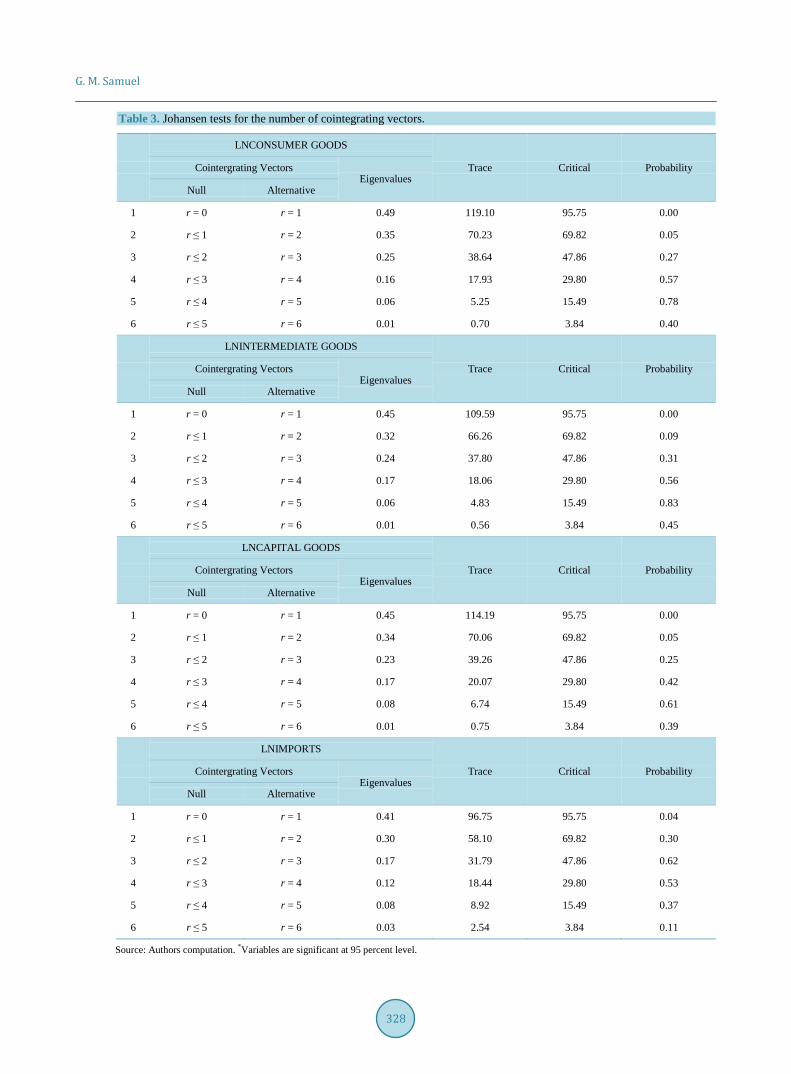
4.4.2. Cointegration Analysis We use the Johansen-Juselius procedure to test for cointegration, this procedure is also known as the Full-In- formation Maximum Likelihood Approach (FIML). This procedure is a vector auto regression based test that is conducted to establish the combination of variables that are cointegrated. Prior to undertaking any cointegration tests, we first specify the appropriate order of lags (p) of the Vector Autoregression (VAR) model. The lag order is determined using the Schwarz Information Criterion. By doing this, we find that the optimum lag length is equal to 2. Having established the optimum lag length, we proceed by performing the cointegration test. [17] recommend the J-Maximal eigenvalues test statistics for establishing the number of cointegration relations. Ta-ble 3 reports the maximum eigenvalue test results.

In Table 3, r denotes the number of cointegrating vectors. Given that the test statistic exceeds its critical value (5%) when the null is r = 0, we can conclude that at least one cointegrating vector is present at the 0.05 level for each of the models. See details in Table 4.

Table 2. Unit root test results.

Augmented Dickey-Fuller (ADF) Test Phillip Perron (PP) Test

Level

Variable Intercept and Trend Intercept and Trend

Aggregate goods −1.323(2) −3.468(1)

Consumer goods −2.449(2) −8.962(1)

Intermediate goods −2.487(1) −2.079(2)

Capital goods −2.593(1) −2.444(1)

GDP −2.553(2) −2.663(3)

REER −5.989(1) −8.034(3)

Foreign Exchange Reserve −1.672(2) −2.021(1)

Average tariff rate −2.113(2) −3.210(1)

First Difference

Variable Intercept and Trend Intercept and Trend

Aggregate goods −3.549(8) −9.773(1)

Consumer goods −3.556(2) −8.985(1)

Intermediate goods −3.749(2) −9.038(1)

Capital goods −3.386(2) −9.031(1)

GDP −3.703(4) −16.190(1)

REER −3.26(3) −8.131(1)

Foreign Exchange Reserve −3.642(6) −9.157(1)

Average tariff rate −3.36(10) −11.241(1)

G. M. Samuel

328

Table 3. Johansen tests for the number of cointegrating vectors.

LNCONSUMER GOODS

Trace Critical Probability Cointergrating Vectors Eigenvalues

Null Alternative

1 r = 0 r = 1 0.49 119.10 95.75 0.00

2 r ≤ 1 r = 2 0.35 70.23 69.82 0.05

3 r ≤ 2 r = 3 0.25 38.64 47.86 0.27

4 r ≤ 3 r = 4 0.16 17.93 29.80 0.57

5 r ≤ 4 r = 5 0.06 5.25 15.49 0.78

6 r ≤ 5 r = 6 0.01 0.70 3.84 0.40

LNINTERMEDIATE GOODS


Null Alternative

1 r = 0 r = 1 0.45 109.59 95.75 0.00

2 r ≤ 1 r = 2 0.32 66.26 69.82 0.09

3 r ≤ 2 r = 3 0.24 37.80 47.86 0.31

4 r ≤ 3 r = 4 0.17 18.06 29.80 0.56

5 r ≤ 4 r = 5 0.06 4.83 15.49 0.83

6 r ≤ 5 r = 6 0.01 0.56 3.84 0.45

LNCAPITAL GOODS


Null Alternative

1 r = 0 r = 1 0.45 114.19 95.75 0.00

2 r ≤ 1 r = 2 0.34 70.06 69.82 0.05

3 r ≤ 2 r = 3 0.23 39.26 47.86 0.25

4 r ≤ 3 r = 4 0.17 20.07 29.80 0.42

5 r ≤ 4 r = 5 0.08 6.74 15.49 0.61

6 r ≤ 5 r = 6 0.01 0.75 3.84 0.39

LNIMPORTS


Null Alternative

1 r = 0 r = 1 0.41 96.75 95.75 0.04

2 r ≤ 1 r = 2 0.30 58.10 69.82 0.30

3 r ≤ 2 r = 3 0.17 31.79 47.86 0.62

4 r ≤ 3 r = 4 0.12 18.44 29.80 0.53

5 r ≤ 4 r = 5 0.08 8.92 15.49 0.37

6 r ≤ 5 r = 6 0.03 2.54 3.84 0.11

Source: Authors computation. *Variables are significant at 95 percent level.

G. M. Samuel

329

The variables in the equation for the aggregate import (LnM), Consumer goods (LnC), Intermediate goods (LnI) and capital goods (LnK) models have two cointergrating vectors each. The results of the cointegration test suggest that there is a long-run dynamic causal relationship between the endogenous variables for the aggregate imports (LnM), intermediate goods (LnI), Consumer goods (LnC) and capital goods (LnK) models. This is ex-pected because most of Uganda’s Consumer, Intermediate and Capital goods, depend on macroeconomic varia-ble such as GDP, Relative Import Price, Exchange Rate Reserves and Openness.

A normalizing restriction is imposed on the import variables to determine the cointegrating vectors and the adjustment parameters. The cointegration vectors and the adjustment parameters for aggregate import are indi-cated in Table 5. The cointergrating vectors have long-run elasticities of aggregate import demand and the dis-aggregated import models with respect to the real income (LnGDP), trade openness (LnOPEN), real effective exchange rate (LnREER), foreign exchange reserves (LnRESER) and relative import price (LnRPM). The re-sults for the estimated coefficients under the Johansen-Jusellius procedure are similar to results by [11] [14]-[16] [34] who obtained long run import demand elasticities from other studies on developing countries.

4.4.3. Long-Run Estimates The result shows that the disaggregate and aggregate import demand models have a long run relation with GDP, trade openness, real effective exchange rate, foreign exchange rate reserves and relative import price.

1) Consumer Goods Import Demand Function The results show that GDP, real effective exchange rate and relative import price are important long run de-

terminants of consumer goods import demand for Uganda. The elasticities are 0.5399, −0.723 and 0.356 respec-tively. All the elasticities are statistically significant at 5 percent level of significance. The consumer goods Table 4. Cointegrating vectors and optimum lag order using Johansen tests.

Variable Number of Cointegrating Lag Order

1 LNCONSUMER 2 2

2 LNINTERMEDIATE 1 2

3 LNCAPITAL 2 2

4 LNIMPORT 1 2

Source: Authors computation. Table 5. Estimated cointegrated vector in Julius Johansen.

Variables LNM LNGDP lnOPEN LNREER LNRESER LNRPM

Cointegrating Eqn 1 0.402467 −1.22803* −0.401447* 0.07846 −0.09792*

Standard errors −0.21005 −0.19805 −0.16702 −0.15565 −0.04473

Variables LNC LNGDP lnOPEN LNREER LNRESER LNRPM

Cointegrating Eqn 1 0.53999* −0.65142* −0.72303* −0.88412* 0.35613*

Standard errors −0.26526 −0.24903 −0.21481 −0.19898 −0.07076

Variables LNI LNGDP lnOPEN LNREER LNRESER LNRPM

Cointegrating Eqn 1 0.341547 −0.76441* −0.80291* −0.75672* 0.58387*

Standard errors −0.35694 −0.3294 −0.28289 −0.25586 −0.1282

Variables LNK LNGDP lnOPEN LNREER LNRESER LNRPM

Cointegrating Eqn 1 1.18237* −1.28332* −0.682075 −0.95814* 0.49354*

Standard errors −0.43742 −0.40999 −0.35108 −0.32356 −0.13725

Source: Authors computation. *Variables are significant at 95 percent level.

G. M. Samuel

330

import demand is negatively related to real effective exchange rate while positively related to income of the country and the relative import price. As far as the relative strength of the variables in influencing the aggregate import demand is concerned, real effective exchange rate comes out to be the most influential determinant of consumer goods.

2) Intermediate Goods Import Demand Function The elasticities for GDP, real effective exchange rate, exchange rate reserve and relative import price are sta-

tistically significant at 5 percent level of significance. The elasticities are 0.341, −0.7644, −0.802, −0.0756 and 0.583 respectively. This shows that the coefficients are important determinants of long run intermediate goods import demand. The intermediate goods import demand is negatively related to trade openness, real effective exchange rate and foreign exchange rate reserve while positively related to the relative import price. As far as the strength of the variables in influencing import demand, real effective exchange rate has highest elasticity, followed by trade openness, foreign exchange rate reserves and relative import price. The findings are in line with the study expectations as well as economic theory.

3) Capital Goods Import Demand Function The elasticities for GDP and real effective exchange rate are statistically significant at 5 percent level of sig-

nificance, the elasticities are 1.182 and 1.283 respectively. The other variables are in the model are insignificant. This suggests that GDP and trade openness are the only determinants of capital goods import demand in the long run. GDP has the highest elasticity on capital goods, followed by the real effective exchange rate.

4) Aggregate Goods Import Demand Function The elasticities for trade openness, real effective exchange rate and relative import price are statistically sig-

nificant at 5 percent level of significance. The elasticities are −1.228, −0.401 and 0.097 respectively. The elas-ticities for GDP and exchange rate reserves are statistically insignificant indicating they don’t influence import demand. This shows that trade openness, real effective exchange rate and relative import price are important de-terminants of aggregate import for Uganda in the long run. Trade openness and real effective exchange rate is negatively related to aggregate import demand while positively related to relative import price. As far as the rel-ative strength of the variables in influencing the aggregate import demand is concerned trade openness comes out to be the most influential determinant of import, followed by foreign exchange reserve and relative import price. These results are similar to findings by [8] and [14].

4.4.4. Error Correction Models From results presented in the Cointergration analysis, the presence of a cointegrating vector together with the evidence of weak exogeneity suggests that we can use a single-equation error-correction representation without the loss of the ability to perform proper inferences. The single-equation error-correction representation is used to determine how well the dynamic adjustment process generates Uganda’s level of disaggregated and aggregate import demand.

Using the single-equation error-correction representation, we develop an error correction model to ascertain the short-run dynamics of the disaggregate import demand models for consumer goods, intermediate goods and capital goods as well as the aggregate demand goods model. A general-to-simple methodology is adopted by specifying an over-parameterized error correction model, as in Equation (3.13). The over-parameterized model is reduced to a parsimonious error correction model based on the Akaike Information Criterion (AIC), F-statistic, Durbin-Watson, Serial correlation test and the R squared tests. The preferred model for the disaggregated import demand are provided in Tables 6-8 and Table 9. Representing the consumer, intermediate, capital and aggregate import demand goods respectively.

The import demand models specified below:

0 1 2 1 3 40 0 0 0

5 6 7 80 0 0 0

9 100 0

LnM LnGDP LnGDP LnOPEN LnOPEN

LnREER LnREER LnRES LnRES

LnRPM LnR M ,P

p p p pit i it i it i it i it ii i i i

p p p pi it i it i i it i t ii i i i

p pi t i it i iti i U

− −= = = =

− −= = = =

−= =

∝ + ∝ + ∝ + ∝ + ∝

+ ∝ + ∝ + ∝ + ∝

+ ∝ + +

=

∝

∑ ∑ ∑ ∑∑ ∑ ∑ ∑∑ ∑

(3.14)

Table 6, presents results for the consumer goods import demand, the coefficient of 1ecmt− is found to be 0.418 and statistically significant at the 5 percent level. This confirms the existence of a long run relationship between the dependent and independent variables. The coefficient of the lagged ecm term suggests a slower adjustment

G. M. Samuel

331

Table 6. Error-correction model for consumer goods import demand.

Variable Coefficient Std. Error t-Statistic Prob.

LC(−1) 0.462 0.155 2.974 0.004

LGDP 1.147 0.283 4.057 0.000

LRPM −0.029 0.014 −2.054 0.044

LOPEN(−1) −0.188 0.079 −2.383 0.020

LREER 1.175 0.354 3.322 0.001

ECM(−1) 0.418 0.161 2.606 0.011

C −14.051 3.805 −3.692 0.000

R-squared 0.98241 Mean dependent var 13.0768

Adjusted R-squared 0.98085 S.D. dependent var 0.61891

S.E. of regression 0.08564 Akaike info criterion 1.98859

Sum squared resid 0.49875 Schwarz criterion 1.77229

Log likelihood 81.5721 Durbin-Watson stat 1.92105

Source: Authors computation. process. This implies that 41 percent of the disequilibrium of the previous period’s shock adjusts back to the long run equilibrium in the current period. The estimated coefficients of LC (−1), LGDP, LRPM, LOPEN (−1) and LREER in Table 6 represent the short-run elasticities for lagged consumer goods import demand, income elasticity, relative import price, lagged trade openness and real effective exchange rate elasticity. The coeffi-cients are statistically significant at the 5 percent level of significance.

The coefficient for the short-run income elasticity is 1.147, this is higher than the long-run coefficient which stands at 0.539. The size of the coefficient is greater than one and is elastic, this shows that GDP has a high in-fluence on consumer goods in the short run compared to the long run. The estimated coefficient indicates that a 1 percent change in income leads to approximately 1.147 percent change in the level of imported consumer goods. The result is consistent with the expected sign. The income elasticity under the consumer goods import demand model shows a higher elasticity than the income elasticity under the aggregate import demand model. This shows that GDP has a high influence on consumer goods.

The short-run relative import price elasticity is −0.029 and statistically significant at the 5 percent level, this is smaller than the long-run coefficient which stands at 0.356. This indicates that the relative import price is nega-tive in the short run while positive in the long run. The estimated coefficient indicates that a 1 percent change in the relative import price leads to approximately −0.029 percent change in the level of consumer goods import demand. This is in line with economic theory which suggests that an increase in import prices would lead to a reduction import volumes on account of an increase in prices. The finding is meaningful for small open coun-tries that are associated with lower participation in international trade.

The estimate for the short-run real effective exchange rate is 1.175 and statistically significant at the 5 percent level. The estimate is greater than unity and stronger than the long-run elasticity which stands at −0.723. This implies that the effect of a change in real effective exchange rate on the volume of imports is positive in the short run while in the long run it’s weaker and negative. This suggests that the demand for consumer goods is more sensitive to foreign exchange availability in the short run compared to the long run.

The coefficient for the first lag of consumer goods import demand is 0.46 and statistically significant at the 5 percent level. The estimated coefficient indicates that a 1 percent change in the first lag of consumer goods im-port demand leads to approximately −0.46 percent change in the level of consumer goods imports. The result is consistent with the expected sign suggesting that, consumer goods import in the previous period have influence consumer import demand in the current period. In addition first lag of trade openness is −0.188 and statistically significant at the 5 percent level, suggesting that trade openness in the previous period influences consumer im-port demand in the current period.

Table 7, presents results for the intermediate goods import demand, the coefficient of 1ecmt− is found to be 0.21 and statistically significant at the 5 percent level. This implies that 21 percent of the disequilibrium of the

G. M. Samuel

332

Table 7. Error-correction model for intermediate goods import demand.


LI(−1) 0.686 0.116 5.887 0.000

LGDP 0.510 0.182 2.802 0.007

LRPM −0.030 0.015 −1.988 0.051

LREER(−1) 0.652 0.292 2.234 0.029

ECM(−1) 0.210 0.141 1.485 0.142

C −7.104 2.902 −2.448 0.017






Source: Authors computation. previous period’s shock adjusts back to the long run equilibrium in the current period. The coefficient of the lagged ECM term suggests a slower adjustment process. This implies that 21 percent of the disequilibrium of the previous period’s shock adjusts back to the long run equilibrium in the current period.

The estimated coefficients of LI (−1), LGDP, LRPM and LREER (−1) in Table 7 represent the short-run elasticities for lagged intermediate goods import demand, income elasticity, relative import price and lagged real effective exchange rate elasticity.

The coefficient for the short-run income elasticity is 0.510, this is similar to the long-run coefficient which stands at 0.341. The size of the coefficient is significant and inelastic in both the short and long run. The esti-mated coefficient indicates that a 1 percent change in income leads to approximately 0.510 percent change in the level of intermediate goods import demand. This shows that GDP has a comparable influence in both the short run and the long run. The result has the expected sign and it’s in line with economic theory.

The estimate for the short-run relative import price elasticity is −0.030 and statistically significant at the 5 percent level, this is lower than the long-run coefficient which stands at 0.583. The estimated coefficient indi-cates that a 1 percent change in the relative import price leads to approximately −0.030 percent change in the level of intermediate goods import demand. The results suggest that relative price elasticity of intermediate goods is in the range of inelastic i.e., demand for intermediate goods seems to be less sensitive to price changes. As such a reduction in import price has little effect on intermediate goods import demand, the result has the ex-pected sign and it’s in line with the study’s prediction.

The estimate for the short-run real effective exchange rate is 0.652 and statistically significant at the 5 percent level. The short-run estimate is stronger than the long-run elasticity which stands at −0.802. The estimated coef-ficient indicates that a 1 percent change in real effective exchange rate leads to approximately 0.652 percent change in the level of import volumes. The short-run coefficient is inelastic and suggests a positive impact on import demand. This implies that the demand for intermediate goods is less sensitive to foreign exchange avail-ability in Uganda. The coefficient for the first lag of intermediate goods import demand is 0.686 and statistically significant at the 5 percent level. The inelastic coefficient shows that import in the previous period influences import demand in the current period.

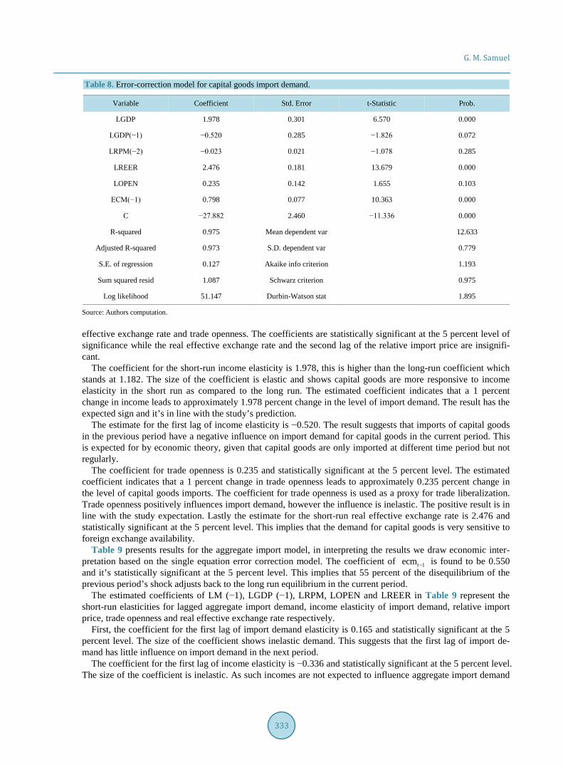
Table 8, presents results for the capital goods import demand, the coefficient of 1ecmt− is found to be 0.79 and statistically significant at the 5 percent level. This implies that 79 percent of the disequilibrium of the pre-vious period’s shock adjusts back to the long run equilibrium in the current period. The coefficient of the lagged ecm term suggests a faster adjustment process.

The estimated coefficients of LGDP, LGDP (−1), LRPM (−2), LREER and LOPEN in Table 8 represent the short-run elasticities for income elasticity, first lag of income elasticity, second lag of relative import price, real

G. M. Samuel

333

Table 8. Error-correction model for capital goods import demand.


LGDP 1.978 0.301 6.570 0.000

LGDP(−1) −0.520 0.285 −1.826 0.072

LRPM(−2) −0.023 0.021 −1.078 0.285

LREER 2.476 0.181 13.679 0.000

LOPEN 0.235 0.142 1.655 0.103

ECM(−1) 0.798 0.077 10.363 0.000

C −27.882 2.460 −11.336 0.000






Source: Authors computation. effective exchange rate and trade openness. The coefficients are statistically significant at the 5 percent level of significance while the real effective exchange rate and the second lag of the relative import price are insignifi-cant.

The coefficient for the short-run income elasticity is 1.978, this is higher than the long-run coefficient which stands at 1.182. The size of the coefficient is elastic and shows capital goods are more responsive to income elasticity in the short run as compared to the long run. The estimated coefficient indicates that a 1 percent change in income leads to approximately 1.978 percent change in the level of import demand. The result has the expected sign and it’s in line with the study’s prediction.

The estimate for the first lag of income elasticity is −0.520. The result suggests that imports of capital goods in the previous period have a negative influence on import demand for capital goods in the current period. This is expected for by economic theory, given that capital goods are only imported at different time period but not regularly.

The coefficient for trade openness is 0.235 and statistically significant at the 5 percent level. The estimated coefficient indicates that a 1 percent change in trade openness leads to approximately 0.235 percent change in the level of capital goods imports. The coefficient for trade openness is used as a proxy for trade liberalization. Trade openness positively influences import demand, however the influence is inelastic. The positive result is in line with the study expectation. Lastly the estimate for the short-run real effective exchange rate is 2.476 and statistically significant at the 5 percent level. This implies that the demand for capital goods is very sensitive to foreign exchange availability.

Table 9 presents results for the aggregate import model, in interpreting the results we draw economic inter-pretation based on the single equation error correction model. The coefficient of 1ecmt− is found to be 0.550 and it’s statistically significant at the 5 percent level. This implies that 55 percent of the disequilibrium of the previous period’s shock adjusts back to the long run equilibrium in the current period.

The estimated coefficients of LM (−1), LGDP (−1), LRPM, LOPEN and LREER in Table 9 represent the short-run elasticities for lagged aggregate import demand, income elasticity of import demand, relative import price, trade openness and real effective exchange rate respectively.

First, the coefficient for the first lag of import demand elasticity is 0.165 and statistically significant at the 5 percent level. The size of the coefficient shows inelastic demand. This suggests that the first lag of import de-mand has little influence on import demand in the next period.

The coefficient for the first lag of income elasticity is −0.336 and statistically significant at the 5 percent level. The size of the coefficient is inelastic. As such incomes are not expected to influence aggregate import demand

G. M. Samuel

334

Table 9. Error-correction model for aggregate import demand model.


LM(−1) 0.165 0.090 1.831 0.072

LGDP(−1) −0.336 0.139 −2.411 0.019

LRPM 0.027 0.012 2.175 0.033

LREER 0.271 0.113 2.404 0.019

LOPEN 1.009 0.098 10.340 0.000

ECM(−1) 0.551 0.118 4.669 0.000

C 0.339 1.396 0.243 0.809






Source: Authors computation. in the short run. The result is consistent with the expected sign and findings by [15] who finds a similar results for 70 developing countries of which Uganda is included.

The estimate for the short-run price elasticity is 0.027 and statistically significant at the 5 percent level. The estimate is similar to the long-run elasticity which stands at 0.097. This suggests that the short run price change is inelastic and positive in both the short run and the long run. This result has the expected sign and is consistent with results from [31].

The coefficient for the short-run trade openness is 1.009 and statistically significant at the 5 percent level, this differs from the long-run coefficient which stands at −1.228. The estimate suggests that trade openness is elastic and positively influences import demand in the short run while in the long run it’s inelastic. The estimated coef-ficient indicates that a 1 percent change in trade openness leads to approximately 1.009 percent change in the level of imports. The result is consistent with the expected sign and the likely explanation for this is, is the fact that trade liberalization increases import demand. This result agrees with results from [19] who established that trade openness positively influences aggregate import demand in Ghana.

The estimate for the short-run real effective exchange rate elasticity is 0.271 and statistically significant at the 5 percent level. The estimate differs from the long-run elasticity which stands at −0.401. The estimated coeffi-cient indicates that a 1 percent change in real effective exchange rate leads to approximately 0.271 percent change in the level of imports. The size of the coefficient is inelastic and shows a relatively small impact on ag-gregate import demand. This result does not have the expected sign and is inconsistent with literature. The possible explanation could be attributed to aggregation bias since the disaggregate models have the expected signs.

4.5. Conclusion This chapter investigates the disaggregated import demand functions for Uganda during the period 1994-2012, it categorizes imports into four groups namely; consumer goods, intermediate goods, capital goods and aggregate goods. The main aim of the chapter is to estimate disaggregated import demand in the post-liberalization period. The demand function is based on traditional import demand function by [11]. Nevertheless, following the litera-ture and work by [14] [35], the model is modified to include trade openness, foreign exchange rate reserves and foreign exchange availability as an explanatory variable in the import demand functions.

First results reveal that the consumer, intermediate, capital and aggregate import volumes are cointegrated with Uganda’s relative import price, income, real effective exchange rate, trade openness and foreign exchange

G. M. Samuel

335

rate reserves. The coefficient on relative import price under the consumer goods and intermediate goods model is statistically significant. Under capital goods the coefficient on relative import price is statistically insignificant for both the short-run and long-run models. The relative import price elasticity of the two disaggregated catego-ries is in the inelastic range for the short run and long run, implying that the demand for consumer goods and in-termediate goods is less sensitive to changes in import prices.

Secondly foreign exchange availability is statistically significant in consumer goods, intermediate goods and capital goods demand function for the short run. The coefficient on foreign exchange is statistically significant for all four categories under the long run models. In the intermediate import demand function, foreign exchange availability turns out to be inelastic. This indicates that intermediate goods import demand is less sensitivity to foreign exchange availability. Under the consumer and capital goods import demand functions, the foreign ex-change availability turns out to be elastic in the short run. This indicates that capital goods import demand is more sensitivity to foreign exchange availability in the short run.

Despite the perceived importance of income in the aggregate demand function, the coefficient value yields in-significant results in both the short and long run, however under the three disaggregate models the coefficient is significant. The capital and consumer import demand model turn out to be elastic. This indicates strong sensitiv-ity of both capital and consumer goods import demand to GDP in both the short and long run. The intermediate goods import demand model turn out to be inelastic indicating less sensitivity of intermediate goods to GDP in both the short and long run.

The coefficient value for trade openness is above unity and statistically significant for capital goods in the short run. This indicates high sensitivity of trade openness to capital goods in the short run. On the other hand the trade openness coefficient under the consumer and intermediate goods import demand functions are statisti-cally insignificant and as such they don’t influence import demand.

The estimated short-run dynamic specification shows that Uganda’s consumer, intermediate and capital goods import volumes is largely explained by the country’s relative import price, GDP and real effective exchange rate. The long run elasticities are different from the short-run elasticities, although the short-run elasticity appears more responsive to import demand compared to the long run elasticity. The results are consistent with other stu-dies by [8] [14] [16] [23] [36], which generally find that developing countries tend to have significantly higher short-run elasticities. The coefficient for real effective exchange rate and trade openness is positive and shows that trade liberalization increases import demand.

4.6. Policy Implications The results bear out policy implications. First the short-run and long-run income elasticity for consumer, inter-mediate and capital goods import demand turns out to be elastic, indicating strong sensitivity of these import categories to income in both the short run and the long run. This result shows that Uganda is highly dependent on the imports of consumer, intermediate goods and capital goods which are required in the production process, particularly production for exports. In order to prevent a trade deficit and related negative impacts caused by imports from the world market, Uganda should strengthen its domestic economy, especially its manufacturing sector to reduce on these imports. Secondly the elasticities in the three disaggregated import categories appear more responsive to import demand compared to aggregate import demand function. The policy suggestion is that government should consider using disaggregated analysis in designing and evaluations of import policies.

Acknowledgements I would also like to express my gratitude to Associate Professors Eria Hisali and Edward Bbaale for the very helpful comments and constructive suggestions on econometric analysis.

References [1] Jaimovich, D. and Kamuganga, D. (2010) Three Decades of Trade Policy in Uganda: Two Generations of Reforms in

the Quest to Become Part of the Global Market. Department of Applied Econometrics and International Economic Policy, Goethe University. c.

[2] Blejer, M. and Cheasty, A., (1990) Fiscal Implications of Trade Liberalization. In: Tanzi, V., Ed., Fiscal Policy in Open Developing Economies, International Monetary Fund, Washington DC.

G. M. Samuel

336

[3] Khattry, B. and Rao, J.M. (2002) Fiscal Faux Pas? An Analysis of the Revenue Implications of Trade Liberalization. World Development, 30, 1431-1444. http://dx.doi.org/10.1016/S0305-750X(02)00043-8

[4] Mwase, N.R.L. (1990) Liberalizing Foreign-Exchange Rates in Sub-Saharan Africa: A Comment. Development Policy Review, 8, 83-86. http://dx.doi.org/10.1111/j.1467-7679.1990.tb00148.x

[5] Brownbridge, M. and Tumusiime-Mutebile, E. (2006) Aid and Fiscal Deficits: Lessons from Uganda on the Implica-tions for Macroeconomic Management and Fiscal Sustainability. Development Policy Review, 25, 193-213. http://dx.doi.org/10.1111/j.1467-7679.2007.00366.x

[6] Kilimani, N. and Sebagala, R, (2009) Trade Liberalization, Export and Import Growth: Evidence from Uganda. CSAE Working Paper.

[7] Omolo, S.W. (1992) Bilateral Trade between Kenya and Uganda: An Empirical Investigation. Master’s Thesis, Uni-versity of Nairobi, Nairobi. http://erepository.uonbi.ac.ke:8080/xmlui/handle/123456789/20300

[8] Abuka, C.A and Ddamulira, D.M. (1999) Import Demand in Uganda: An Investigation, 1987-1996. Bank of Uganda Staff Papers, Vol. 1, No. 1, December 1999.

[9] Grossman, G. M. and Helpman, E. (1991) Trade, Knowledge Spillovers and Growth. European Economic Review, 35, 517-526. http://dx.doi.org/10.1016/0014-2921(91)90153-A

[10] Hong, P. (1999) Import Elasticities Revisited. Discussion Paper No. 10, Department of Economic and Social Affairs, New York.

[11] Goldstein, M. and Khan, M.S. (1985) Income and Price Effects in Foreign Trade. In: Jones, R.W. and Kenen, P.B., Eds., Handbook of International Economics, Elsevier Science Publications, New York, Vol. II, 1041-1105.

[12] Junz, H. and Rhomberg, R.R. (1973) Price Competitiveness in Export Trade among Industrial Countries. American Economic Review, Papers and Proceedings, 63, 412-418.

[13] Tang, T.C. (2003) An Empirical Analysis of China’s Aggregate Import Demand Functions. China Economic Review, 12, 142-163. http://dx.doi.org/10.1016/S1043-951X(03)00021-X

[14] Dutta, D. and Nasir Uddin, A. (2004) An Aggregate Import Demand Function for India: A Cointegration Analysis. Ap-plied Economics Letters, 11, 607-613. http://dx.doi.org/10.1080/1350455042000271134

[15] Ho, W.S. (2004) Estimating Macao’s Import Demand Functions. Monetary Authority of Macao, 18. [16] Santos-Paulino, A. and Thirlwall, A.P. (2004) The Impact of Trade Liberalisation on Exports, Imports and the Balance

of Payment of Developing Countries. The Economic Journal, 114, F50-F72. [17] Sarmad, K. (1989) The Determinants of Import Demand in Pakistan. World Development, 17, 1619-1625. [18] Melo, O. and Vogt, M.G. (1984) Determinants of the Demand for Imports of Venezuela. Journal of Development Eco-

nomics, 14, 351-358. http://dx.doi.org/10.1016/0304-3878(84)90064-6 [19] Gumede, V. (2000) Import Demand Elasticities for South Africa: A Cointegration Analysis. Journal for Studies in

Economics and Econometrics, 24, 21-37. [20] Aydin, M., Ciplak, U. and Yucel, E. (2004) Export Supply and Import Demand Models for the Turkish Economy. Re-

search Department Working Paper, the Central Bank of the Republic of Turkey, No. 04/09, 107-123. [21] Clarida, R.H. (1994) Cointegration, Aggregate Consumption, and the Demand for Imports: A Structural Econometric

Investigation. The American Economic Review, 84, 298-308. [22] Senhadji, A. (1998) Time-Series Estimation of Structural Import Demand Equations: A Cross-Country Analysis. IMF

Staff Papers, 45, 236-268. http://dx.doi.org/10.2307/3867390 [23] Dash, A.K. (2006) An Econometric Estimation of the Aggregate Import Demand Function for India. The ICFAI Jour-

nal of Applied Finance, 12, 30-40. [24] Zaramba, E. (2010) Price and Income Elasticities of Crude Oil Import Demand in South Africa: A Cointegration Anal-

ysis. Energy Policy, 38, 7844-7849. http://dx.doi.org/10.1016/j.enpol.2010.08.044 [25] Mwega, F.M. (1993) Import Demand Elasticities and Stability during Trade Liberalization: A Case Study of Kenya.

Journal of African Economies, 2, 381-416. [26] Giovanetti, G. (1989) Aggregate Imports and Expenditure Components in Italy: An Econometric Analysis. Applied

Economics, 21, 957-971. http://dx.doi.org/10.1080/758518236 [27] Aizenman, J. and Jinjarak, Y. (2009) Globalisation and Developing Countries—A Shrinking Tax Base? Journal of De-

velopment Studies, 45, 653-671. http://dx.doi.org/10.1080/00220380802582338 [28] Baunsgaard, T. and Keen, M. (2009) Tax Revenue and (or?) Trade Liberalization. IMF Working Paper 2005-112. Journal

of Public Economics, 94, 563-577. [29] Ebrill, L., Stotsky, J. and Gropp, R. (1999) Revenue Implication of Trade Liberalization. IMF Occasional Paper No. 180.

http://dx.doi.org/10.1016/S0305-750X(02)00043-8

http://dx.doi.org/10.1111/j.1467-7679.1990.tb00148.x

http://dx.doi.org/10.1111/j.1467-7679.2007.00366.x

http://erepository.uonbi.ac.ke:8080/xmlui/handle/123456789/20300

http://dx.doi.org/10.1016/0014-2921(91)90153-A

http://dx.doi.org/10.1016/S1043-951X(03)00021-X

http://dx.doi.org/10.1080/1350455042000271134

http://dx.doi.org/10.1016/0304-3878(84)90064-6

http://dx.doi.org/10.2307/3867390

http://dx.doi.org/10.1016/j.enpol.2010.08.044

http://dx.doi.org/10.1080/758518236

http://dx.doi.org/10.1080/00220380802582338

G. M. Samuel

337

[30] Phillips, E.C.B. and Perron, P. (1988) Testing for a Unit Root in Time Series Regression. Biometrika, 75, 335-346. http://dx.doi.org/10.1093/biomet/75.2.335

[31] Dickey, D.A. and Fuller, W.A. (1981) Likelihood Ratio Statistics for Autoregressive Time Series with a Unit Root. Econometrica, 49, 1057-1072. http://dx.doi.org/10.2307/1912517

[32] Asteriou, D. (2006) Applied Econometrics: A Modern Approach Using Eviews and Microfit. Palgrave Macmillan, Ba-singstoke.

[33] Engle, R.F. and Granger, C.W.J. (1987) Co-Integration and Error Correction: Representation, Estimation, and Testing. Econometrica, 55, 251-276. http://dx.doi.org/10.2307/1913236

[34] Harvey, S. and Sedegah, K. (2011) Import Demand in Ghana: Structure, Behaviour and Stability. AERC Research Pa-per No. 233.

[35] Frimpong, J.M. and Oteng-Abayie, E.F. (2006) Aggregate Import Demand and Expenditure Components in Ghana: An Econometric Analysis. MPRA Paper, No. 599.

[36] Cheung, Y.-W. and Lai, K.S. (1993) A Fractional Cointegration Analysis of Purchasing Power Parity. Journal of Business and Economic Statistics, 11, 103-112.

http://dx.doi.org/10.1093/biomet/75.2.335

http://dx.doi.org/10.2307/1912517

http://dx.doi.org/10.2307/1913236

trade liberalization and disaggregated import demand in...

Documents