trading costs and returns for us equities: estimating high
TRANSCRIPT

Trading Costs and Returns for US Equities: Estimating high-frequency measures of liquidity
from low-frequency data
Joel Hasbrouck
Department of Finance Stern School of Business
New York University 44 West 4th St. Suite 9-190 New York, NJ 10012-1126
212.998.0310
This draft: February 3, 2005
Preliminary draft Comments welcome
David Easley, Maureen O’Hara, Soren Hvidkjaer, Charles Jones, and Ronnie Sadka generously shared their liquidity estimates. This should not be construed as implying approval or endorsement of the present paper.
For comments on an earlier draft, I am grateful to Yakov Amihud, Lubos Pastor, Bill Schwert and seminar participants at the University of Rochester, the NBER Microstructure Research Group, the Federal Reserve Bank of New York, Yale University, and the University of Maryland. All errors are my own responsibility.
The latest version of this paper and a SAS dataset containing the long-run Gibbs sampler estimates are available on my web site at www.stern.nyu.edu/~jhasbrou.

Trading Costs and Returns for US Equities: Estimating high-frequency measures of liquidity
from low-frequency data
Abstract This study examines various measures of trading costs estimated from high-
frequency (TAQ) data and the extent to which these measures can be estimated from
daily data (CRSP). The high-frequency measures tend to be positively correlated. Posted
spreads and effective costs are very highly correlated. Price impact measures and other
statistics derived from dynamic models, however, are only modestly correlated. Among
the set of proxies constructed from daily data, a Gibbs estimate of the effective cost based
on Roll (1984) stands out, achieving a correlation of 0.944 with the corresponding TAQ
estimate. A variant of the illiquidity measure suggested by Amihud (2002) is the best
proxy for the price impact coefficient (a correlation of 0.721 with the TAQ measure).
Both the Gibbs estimate of effective cost and the illiquidity ratio covary positively with
risk-adjusted returns, but the relations exhibit marked seasonality and are not robust to
the use of alternative measures of correlation.
JEL classification codes: C15, G12, G20

Page 1
1. Introduction
As liquidity and transaction costs have become more important in empirical asset pricing
and corporate finance research, the limitations of the high-frequency data samples conventionally
used to estimate these costs have become more apparent. While the CRSP daily file begins in
1962, for example, the corresponding trade and quote databases start in 1983 (at the earliest) and
encompass many different trading and reporting regimes. The construction of historical liquidity
estimates from return data of daily (or longer) frequency therefore stands as an important goal.
This paper broadly advances this line of inquiry. In a comparison sample of US equity data for
which we possess both high-frequency and daily data, the paper surveys the joint behavior of
transaction cost/liquidity measures estimated from the former and proxies computed from the
latter. The analysis establishes guidelines for the subsequent use of the proxies.
As no single measure summarizes all the attributes of “liquidity,” the high-frequency
estimates reflect diverse approaches. From a narrow perspective, an individual trader projecting
the cost of achieving a particular position may compare the expected trade price to some pre-
trade benchmark. This suggests measuring the trading cost as half the posted or effective spread,
for orders accomplished in a single trade. Execution strategies that span multiple orders,
however, must take into account the impacts of early trades on the prices obtained in later trades.
To capture these effects, the present study examines estimates of the trade impact coefficient
from a dynamic model of trades and prices.
Liquidity may also be more broadly defined as reflecting the distortions in prices and
holdings resulting from the trading process. Grossman and Miller (1987) suggest that dealers
smooth the asynchronous demands of customers. The dealers’ accommodation of a one-sided
order flow induces a price change that is subsequently reversed. This reversal is usually
estimated on the basis of (unsigned) volume data (Campbell, Grossman and Wang (1993);
Llorente, Michaely, Saar and Wang (2002); Pastor and Stambaugh (2003)). The present study
describes a representative reversal measure based on signed order flows.

Page 2
Most of the analyses in the paper are based on a sample of 250 firms per year, from 1993
to 2003. Comparisons between high-frequency and daily estimates are possible in this period
because we possess both sorts of data. In this comparison sample all measures, whether
computed from daily or high-frequency data, exhibit numerous extreme values, with some of the
kurtosis coefficients on the order of a thousand or more. Although some of these may be artifacts
of sampling or data errors, it is also likely that the extreme values arise from large cross-sectional
variation in actual trading costs.
The high-frequency liquidity estimates do not uniformly agree. Within the set of
measures consisting of average intraday spread, the closing spread and the effective cost have
correlations of about 0.95. Partial correlations, which control for price level, market
capitalization and volatility, are only slightly lower (around 0.9). Correlations involving the
impact coefficients and reversal measures, however, are much more variable. Thus, there is no
overall concordance, and no single measure that captures all dimensions of liquidity. Stoll (2000)
arrives at similar conclusions, using a panel of liquidity measures that partially
The literature suggests various approaches to estimating high-frequency measures from
returns and unsigned volumes observed at a daily frequency. The effective cost is most
conveniently estimated using the Roll (1984) model. The usual estimate is a moment estimate
computed as the square root of (minus) the first-order return autocovariance. In the frequently-
encountered case where the sample autocovariance is positive, however, this estimate is
infeasible. As an alternative, Hasbrouck (2004) suggests a Gibbs estimate. This approach adopts
a Bayesian perspective and incorporates a prior restriction of a non-negative effective cost.
Daily proxies for high-frequency impact and reversal coefficients are less direct,
however, because total trading volume is quite different from net signed order flow. Proxies for
the price impact coefficient include the Amivest liquidity ratio (Cooper, Groth and Avera (1985))
and the Amihud (2002) illiquidity measure, both of which involve ratios of trade volumes to
absolute returns. The reversal measure suggested by Pastor and Stambaugh (2003) is based on a

Page 3
specification in which the daily return is regressed against lagged total volume signed by the
lagged excess return. This latter quantity is, in effect, a proxy for signed net volume.
The core of the paper is an analysis of the correlations between the high-frequency
liquidity estimates and the proxies constructed from daily data. The simple single-trade measures
are relatively easy to proxy. The Roll estimate of the bid-ask spread (with infeasible estimates
set to zero) performs well, achieving a correlation of 0.852 with the average effective cost
computed from high-frequency data. The Gibbs estimate, however, does even better, attaining a
0.944 correlation. The price impact coefficient is more difficult to proxy. Here, the winner is a
square-root variant of the Amihud (2002) illiquidity measure, for which the relevant correlation
is 0.721. The signed reversal measure is yet more difficult, being at best weakly correlated with
the unsigned reversal coefficient.
Having established the strong performance of the Gibbs estimate of effective cost in the
set of comparison firms, the paper then turns to investigation of this measure in other samples.
Analysis of estimates based on the full CRSP daily file indicates that smaller firms on both
NYSE/Amex and Nasdaq have effective costs that are on average high (one to two percent) and
quite variable. Effective costs for medium and large firms are substantially lower and less
variable. Despite the strong performance of the Gibbs estimate as a proxy in the cross-section,
however, analysis of the Dow stocks suggests that it does not capture variation in effective cost
when this cost is substantially smaller than the daily price volatility.
As an application, the study examines the relation between the liquidity proxies
calculated for the CRSP daily file and risk-adjusted returns, suggested by Brennan, Chordia and
Subrahmanyam (1998). When risk-adjusted returns are regressed against the proxies
individually, both the Gibbs estimate of the effective cost and the illiquidity ratio are positively
correlated with BCS risk-adjusted returns. These results, however, are not robust. The relations
between liquidity measures and risk-adjusted returns are sensitive to extreme values. Moreover,
these relations exhibit marked seasonality, with January values being the highest. This is
consistent with Eleswarapu and Reinganum (1993).

Page 4
The paper is organized as follows. The next section summarizes measures of trading cost
based on high-frequency trade and quote data. Section 3 describes the proxies constructed from
daily data. Reversal measures, however, are sufficiently distinct to warrant a separate discussion
in Section 4. Section 5 describes the construction of the high-frequency/daily comparison
sample and the estimation details. The properties and interrelations of these measures are
discussed in Section 6. The remaining two sections examine the long-term evidence. Section 8
describes the time-series and cross-section properties of the Gibbs estimates of effective cost in
the CRSP daily data file. Section 9 presents the asset-pricing specifications. A brief summary
concludes the paper in Section 10.
2. Microstructure-based measures of transaction costs and liquidity
This section discusses measures generally motivated by microstructure models and
estimated with high-frequency data. The following describes in turn posted and effective spreads,
and impact measures based on dynamic models of prices and trades. Reversal measures are
discussed separately in section 4.
a. Spreads: posted and effective
The implementation shortfall approach of Perold (1988) provides a framework for
imputation of trading costs. This approach focuses on the difference between the actual portfolio
return and the return that would have been achieved had all purchases and sales occurred at
hypothetical prices that were free of trading costs. The difference is the cost of implementing the
strategy.
For a single executed trade this suggests measuring the cost as the difference between the
average transaction price and a hypothetical benchmark price taken prior to the initial trade. One
common benchmark is the midpoint of the bid and ask prevailing at the time of the order
submission. For a trade executed at the bid or ask, the implied cost is one-half the bid-ask spread.
For the spread and related measures, the analysis explores both log and level forms, but with
emphasis on the former. The log spread prevailing before the kth trade is , where ak k ks a b= − k

Page 5
and bk are the log ask and bid prices. The level spread is k kS A Bk= − , where and k kB A are the
bid and ask prices in dollars per share.
In many markets and for a variety of reasons, market orders often transact at prices better
or worse than the posted quotes. This motivates use of the log effective cost, defined for the kth
trade as
(1) , for a buy order, for a sell order
k kk
k k
p mc
m p−⎧
= ⎨ −⎩
where pk is the log trade price and mk is the log quote midpoint prevailing at the time the order
was received. The level effective cost, Ck, is defined analogously. The effective cost is most
meaningful for small market orders that can be accommodated in a single trade. It figures
prominently in US securities regulation. Under SEC rule 11ac1-5, market centers must
periodically report summary statistics of this measure.
Accurate computation of the effective cost requires knowledge of order characteristics,
most importantly the arrival time and direction (buy or sell). Studies of order data are common
(e.g., Keim and Madhavan (1995), Harris and Hasbrouck (1996), Chan and Lakonishok (1993),
and Conrad, Johnson and Wahal (2003)), but none of the samples spans a long history. When
order data are unavailable, the effective cost is often estimated from transaction and quote data.
A trade priced above the midpoint of the bid and ask (prevailing at the time of the trade report or
a brief time earlier) is presumed to be a buy order; a trade priced below the midpoint is presumed
to be a sale. Effective costs computed in this fashion are often used in academic studies (see
Bessembinder and Kaufman (1997) and Bessembinder (2003)).
b. Measures based on dynamic models
Many economic models imply joint dynamics for orders and price changes that involve
both permanent and temporary effects. The former reflect the information content of the order,
with Kyle (1985) and Glosten and Milgrom (1985) exemplifying the two main approaches. The
latter arise from transient liquidity effects, inventory control behavior, price discreteness, etc. In
practical trading situations, the principal advantage of the dynamic models over the single-trade

Page 6
approaches discussed above lies in their ability to project execution costs when trades are
distributed over time.
The literature contains a large number of approaches. The following specification is
representative. The evolution of the log quote midpoint is:
1t t tm m Q utλ−= + + (2)
Here, t indexes five-minute intervals, and Qt is a measure of the cumulative signed order flow
over the interval. Defining as the direction of the kth trade (+1 if buyer-initiated, –1 if seller-
initiated, 0 if indeterminate), the measure used here is the sum kq
tt k N
Q∈
= kq∑ where Nt is the
number of trades in the interval. Alternative specifications that involved signed dollar volume
and signed square-root dollar volume gave similar results and are not reported. The λ coefficient
in Eq. (2) measures the impact of orders on prices.
c. Other measures
Reversal measures quantify the transient effects of order imbalances. While the measures
discussed in the present section are based on high-frequency trade and quote data, however,
reversal measures are usually implemented with daily price and volume data. It will facilitate the
exposition, therefore, to defer discussion of reversal measures until section 4.
Even within the class of high-frequency measures, however, the set described above is,
although representative, far from exhaustive. Easley, Hvidkjaer and O'Hara (2002) estimate
return specifications in which liquidity is measured by the estimated probability of informed
trading, PIN (Easley, Kiefer and O'Hara (1997)). Sadka (2004) estimates permanent and
transitory trade impact coefficients in a dynamic framework similar to, but more comprehensive
than the model given in Eq. (2).

Page 7
3. Transaction cost and liquidity measures based on daily data
Estimation of the measures discussed in the previous section generally requires intraday
quote and trade data. I now turn to measures that can be estimated using daily return and volume
data.
a. Moment estimates of the Roll model, cM and cMZ
Roll (1984) suggested a simple model of the spread in an efficient market. Following the
notation used earlier, the model may be stated as:
1k k
k k
m m uk
kp m c q−= +
= +. (3)
The time subscript, k, can be thought of as indexing successive trades. mk is the log quote
midpoint prevailing prior to the trade, pk is the log trade price, qk is the direction indicator, and c
is the effective cost (cf. Eq. (1)), which is presumed constant. The model may also be specified
using levels in lieu of logs for the price variables. It has essentially the same form under time
aggregation. In particular, although the model is sometimes estimated with transaction data (e.g.,
Schultz (2000)), it was originally applied to daily data, with qt being interpreted as the direction
variable for the last trade of the day. The estimation approaches described below take this
perspective.
The Roll model is usually estimated by method-of-moments. The model implies
( )1 1t t t t t tp m c q m c q c q u− −Δ = + − + = Δ + t
)
, (4)
from which it follows that ( 1,t tc Cov p p −= − Δ Δ . The moment estimate, denoted cM, is the
sample analog of this. It possesses all the usual properties of GMM estimators, including
consistency and asymptotic normality. Moment estimation for this model is relatively easy to
implement and often satisfactory.
cM only exists, however, if the first-order sample autocovariance is negative. In samples
of daily frequency this is often not the case. In annual samples of daily returns, Roll found
positive autocovariances in roughly half the cases. Harris (1990) discusses this and other aspects

Page 8
of this estimator. His results show that positive autocovariances are more likely for low values of
the spread. Accordingly, one simple remedy to the problem is to assign an a priori value of zero.
I define the moment/zero estimate as:
( ) ( )1 1, , if ,
0, otherwiseMZ t t t tCov p p Cov p p
c − −⎧ − Δ Δ Δ Δ ≤⎪= ⎨⎪⎩
0
)u
The corresponding estimates based on a price level model are denoted CM and CMZ.
Gibbs-sampler estimates of the Roll model, cGibbs and CGibbs
Hasbrouck (2004) advocates Bayesian estimation using the Gibbs sampler. To complete
the Bayesian specification, I assume here that ( 2~ . . . 0,d
tu i i d N σ and that the data sample is
{ }1 2, , , Tp p p p≡ … . The prior for c is where the “+” superscript denotes
restriction to the positive domain. The prior for
( 2,~ 0,d
priorcc N σ+ )
2uσ is inverted gamma distribution,
(2 ~ ,d
u IG )σ α β . Numerical values for the prior parameters are discussed in section 5. In the
Bayesian approach, the unknowns comprise both the model parameters { }2, uc σ and the latent
data, i.e., the trade direction indicators { }1, , Tq q q≡ … and the efficient prices { }1, , Tm m m≡ … .
The parameter posterior density ( ), uf c pσ is not obtained in closed-form, but is instead
characterized by a random sample of draws. These draws are constructed by iteratively drawing
from the full conditional distributions. The Gibbs estimate of c, denoted cGibbs, is the sample
mean of the posterior draws. The Gibbs estimate of the level effective cost, denoted CGibbs, is
constructed in a similar fashion.
The Gibbs estimate offers some advantages over the moment estimate. First, the prior can
restrict the effective cost estimates to be positive. Second, within the framework of the model,
the posterior is an exact small sample distribution. A third advantage stems from the CRSP
convention of reporting the midpoint of the closing bid and ask (flagged as a negative value) in
lieu of the transaction price if there are no trades on a particular day.
The implications of the CRSP convention differ for the moment and Gibbs estimates. The
moment estimate is based on the sample return autocovariance, which is proportional to 1t ttr r−∑ .

Page 9
The summand here is ( ) ( )1 1 1t t t t t tr r p p p p− − −= − − 2−
t
. In principle, since the model applies to trade
prices, a term should be included only if it encompasses a sequence of three trade prices. For
many stocks, however, this would drastically reduce the sample size. To avoid this attenuation,
the present study uses all closing prices in the moment estimates irrespective of whether they
represent trades or quote midpoints.
The Gibbs estimate, on the other hand, is easily generalized to accommodate quote
midpoints. Specifically, if a quote midpoint is reported on day t, the trade direction indicator is
set to zero. From Eq. (3), this implies tp m= . Intuitively, this prevents the observation from
contributing directly to the estimate of c, but allows one or both of the adjacent prices to
contribute (assuming that they have valid transaction prices).1
This treatment of the Roll model is almost certainly misspecified in a number of
important respects. Actual samples of stock returns typically contain many more extreme
observations than the normal density plausibly admits. Trade directions are unlikely to be
independent of the efficient price evolution. Realized prices are discrete. The effective cost is
unlikely to be constant within a sample, etc. Hasbrouck (2004) discusses various extensions to
deal with some of these features, but for the sake of computational expediency and programming
simplicity, the present paper uses the most basic form of the sampler.
Lest misspecification appear to be a major concern, it must be emphasized that the Gibbs
estimate (like all daily proxies considered here) is compared against values constructed
independently from high-frequency data. There is accordingly no immediate need to assess the
appropriateness of the model assumptions or implementation procedures. If the Gibbs estimates
are strongly correlated with the corresponding high-frequency values, these concerns are of
secondary importance.
1 Formally, this procedure can be justified by embedding the Roll model in a more general
framework in which observation of a quote midpoint or trade price is determined randomly (and
independently of the other variables).

Page 10
The Gibbs sampler generates random draws from the parameter posterior, thus
characterizing the entire distribution. By tabulating, say, the 0.05 and 0.95 quantile points of the
distribution, one could in principle establish a confidence band for the estimate. Unlike the mean
point estimate, however, the estimated confidence limits cannot easily be validated by
comparison to estimates constructed independently.
b. The (Amivest) liquidity ratio, L
The effective cost estimates discussed in the prior two section use only daily price data.
The remaining measures use volume data as well. This imposes a practical limitation because the
interpretation of reported volume may depend on institutional arrangements. Volume in an order-
driven market (such as the NYSE) is not, for example, generally comparable to volume in a
quote-driven market (such as Nasdaq).
The Amivest liquidity ratio is the average ratio of volume to absolute return:
d dL Vol r= (5)
where the average is taken over all days in the sample for which the ratio is defined, i.e., all days
with nonzero returns. It is based on the intuition that in a liquid security, a large trading volume
may be realized with small change in price. This measure has been used in the studies of Cooper,
Groth et al. (1985), Amihud, Mendelson and Lauterbach (1997), and Berkman and Eleswarapu
(1998), among others. Sample distributions of L often exhibit extreme values. Cooper et al and
Amihud et al use ( )log L in subsequent analysis. The present study employs the square-root
transform in lieu of the log. (Zero values of L can in principle exist.) Furthermore, the transform
is applied to the daily ratios, i.e., before averaging. This transformed variant is defined as
1/ 2d dL Vol= r . (6)
c. The illiquidity ratio, I
Amihud (2002) suggests measuring illiquidity as:
d dI r Vol= (7)

Page 11
where rd is the stock return on day d and Vold is the reported dollar volume. The average is
computed over all days in the samples for which the ratio is defined, i.e. days with nonzero
volume. This measure loosely corresponds to λ in Eq. (2), but whereas λ measures the return
impact of a cumulative signed order flow, I captures the absolute return impact of a cumulative
unsigned volume. This measure is used as a risk factor by Acharya and Pedersen (2002).
Analogously to the liquidity ratio, the square-root variant is defined as
1/ 2d dI r Vol= . (8)
d. Other approaches
The set of daily proxies considered above is representative, but not all inclusive.
Lesmond, Ogden and Trzcinka (1999) propose a measure based on the frequency of no-trade
intervals. Goyenko, Holden, Lundblad and Trzcinka (2005) discuss an estimate derived from
clustering of last sale prices, and suggest that it outperforms the Gibbs estimate at monthly (but
not annual) frequencies.
4. Reversal measures
Reversal measures of liquidity summarize the association between return and lagged
order flow. The intuition is that order flow induces a price adjustment that initially overshoots,
then subsequently reverts to, true value. This might arise, for example, due to inventory
adjustments by market makers.
Drawing on this intuition, Pastor and Stambaugh (2003) suggest estimating liquidity by γ
in the regression (using present notation):
( )1 1 1e e
t t t tr r sign r V Dollartθ ϕ γ− − −= + + + ε (9)
where is the stock’s excess return (over the CRSP value-weighted market return). γ is
expected to be negative, with magnitude increasing with illiquidity. Pastor and Stambaugh
estimate this specification using daily return and volume data.
etr

Page 12
The logic of this specification is most apparent from a specification suggested by Pastor
and Stambaugh that is similar to Eq. (9), but involves signed order flow. In present notation:
( )1e
t t tr X Xφ − tu= − + (10)
Where is the excess return over a market-wide common factor, ut is a firm-specific
component, and Xt is the signed dollar order flow on day t. By comparison with Eq.
etr
(9), it is
apparent that lagged order flow is being proxied by dollar volume, signed by excess
return. Pastor and Stambaugh find that when they simulate data using Eq.
( 1tX − )(10) and estimate via
Eq. (9), φ and the γ estimated from Eq. (9) are very highly correlated. The present study
investigates the correspondence by estimating Eq. (9) from CRSP data, and estimating Eq. (10)
using signed order flow constructed from TAQ data.
5. The comparison sample and estimation
a. Construction of the comparison sample
The comparison sample is a random selection of firm-years for which both TAQ (high
frequency) and CRSP (daily) data are available. For each of the eleven years 1993-2003, 250
firms are chosen at random from the CRSP database. To be eligible for selection in a given year,
a firm has to satisfy the following criteria:
1. The issue is an ordinary common share (CRSP share code 10, 11 or 12).
2. The issue is present in the CRSP database on the last trading day of the year.
3. There is no change of trading venue, ticker symbol or cusip identifier after August of the
year.
The first criterion simply limits the sample to those issues usually considered in asset pricing
tests. The remaining criteria are imposed to ensure reasonable homogeneity in a firm’s trading
characteristics over the year. The selection is made based on information in the CRSP events
file. Of the 2,750 firms selected, two were subsequently determined to have no valid return or

Page 13
price observations for the year, and were dropped from the sample. Of the remaining 2.748 firm-
years, 719 were NYSE listings, 344 were Amex, and 1,785 were Nasdaq.
Asset pricing studies sometimes exclude low-priced stocks (e.g., below five dollars). This
practice is deliberately avoided in the present study. Casual observation suggests that transaction
costs are indeed high for low-price stocks. In investigating the effects of transactions costs,
therefore, the observations corresponding to these firms might well be the most informative.
Some studies also exclude firms where the value of an estimated statistic is determined to be
extreme. There is a sensible rationale for this, in that extreme values often reflect errors or other
features of the data that render the observation inappropriate for the model. These filters are not
used in the present study because considerable anecdotal evidence (as well as the statistics
presented below) suggest that actual transaction costs are highly leptokurtotic. Generally in the
present study, estimates are only excluded (in practice, set to ‘missing’) when the estimate is
based on a small number of observations, and the presumed estimation error would be high. The
discussion now turns to estimation details.
b. Estimation of TAQ-based liquidity measures
Estimates are computed for individual firms using up to a year’s worth of data. The TAQ
quote record is filtered to remove quotes with zero bid or ask, offers greater than five times the
bid and spreads greater than five dollars. Only quotes from a stock’s primary listing exchange are
used, and only quotes posted during regular trading hours. Spreads are first averaged within the
day, weighted by the time the spread was in force (i.e., the time to the next quote revision or
market close). The daily values are then averaged across all days. These average level and log
spreads are denoted S and s, respectively.
The other measures involve transaction as well as quote data. The TAQ transaction
record is filtered to remove all trades with nonstandard settlement or corrections. Trades from all
venues are retained, not just the primary listing exchange. Trades are signed and effective costs
computed using quote midpoints prevailing two seconds prior to the reported trade time. When
there are at least 100 trades in a month, effective cost outliers (observations above the 95th

Page 14
percentile) are removed.2 The effective cost observations are averaged over each month,
weighted by dollar volume of the trade, and these monthly observations are then averaged over
the year. The resulting level and log effective cost estimates are denoted C and c, respectively.
Using quote and signed trade data aggregated over five-minute intervals, Eq. (2)
is estimated for each month in which there are at least twenty-five intervals over which the price
change is non-zero and the cumulative signed-trades are non-zero. The coefficient estimate used
in subsequent analysis is the average of the monthly estimates, and is denoted λ5 min. A similar
specification is estimated where the data are time-aggregated over days. For this estimation the
CRSP daily return is used as the dependent variable, and one estimation is computed using all
the days in the year. The coefficient estimate from this regression is denoted λDay. When there
are fewer than fifty days with non-zero returns, the estimate is dropped from subsequent analysis.
The reversal coefficient φ is estimated in a similar fashion using Eq. (10).
c. Estimation of CRSP-based liquidity measures
The remaining measures are based solely on CRSP price, return and volume data. The
moment estimates of effective cost, cM and cMZ, are estimated using the sample first-order
autocovariance (section 3). If this autocovariance is positive, cM is set to “missing”, and cMZ is set
to zero. The level effective cost estimates CM and CMZ are constructed in a similar fashion.
For the Gibbs estimate, the prior for the effective cost is constructed as a normal
distribution truncate to the positive region, denoted ( )2, 0, PriorcN μ σ+ = . (Note that
2, and Priorcμ σ are merely the parameters of the density. Due to the truncation, the actual mean
and variance of the distribution are different.) For the effective cost and log effective cost
estimates, 2,Priorcσ and 2,Prior
Cσ are both set to unity. In case of the log effective cost, a value of
c=1 for a US equity would be extremely, arguably implausibly, high. So the unit interval (0, 1)
2 The only results in the paper that are sensitive to this trimming are those that deal with daily
estimates of effective cost for the Dow stocks (Section 8.a). Failure to remove extreme values in
this case results in elevated variability of the daily effective cost graph in Figure 1.)

Page 15
would be expected to contain all actual values. Within this region, the normal density does not
exhibit extreme variation. These remarks also apply, although to a lesser degree, for the level
effective cost, C.
Although this prior is fairly broad, it is not completely uninformative. This is deliberate
and necessary. In the Gibbs sampler, simulation of the posterior for c requires estimation via
regression of Eq. (4). This estimation is conditional on simulated values of q. In the process,
there is a possibility that at a particular draw all of the qt are either –1 or +1. In this case, all of
right-hand-side variables in the regression (the Δqt ) are zero. The estimated regression
coefficient is therefore undefined, and the new value of c must be drawn from the prior.
The Gibbs sampler is initialized by setting the trade direction indicators to the sign of the
most recent price change (except for prices reported as quote midpoints). Next, 1,000 sweeps of
the sampler are computed. The first 200 draws are discarded (as a burn-in period, to minimize
start-up effects. Parameter estimates are determined as the mean of the final 800 draws. The
number of sweeps was chosen to achieve a manageable computation time. One thousand draws
would not be considered sufficient in many applications, but experimentation with more draws
did not materially change the estimates.
The liquidity coefficient L and its square-root variant L1/2 are estimated using Eqs. (5) and
(6). The illiquidity coefficients I and I1/2 are estimated using Eqs. (7) and (8). The reversal
coefficient γ is estimated from Eq. (9).
As noted above, although censoring of extreme values per se is not consistent with the
aims of the paper, estimates are dropped when they are based on few observations. Specifically,
moment estimates of the effective cost and log effective cost require at least fifty price
observations. In the development of the estimate, each monthly estimate going into the
overall average is computed subject to a minimum of twenty-five five-minute intervals over
which the price change is non-zero and the cumulative signed-trades are non-zero. L and L1/2
estimates require at least fifty days where the return (the denominator in
5miniλ
(5) or (6)) is nonzero.
Similarly, I and I1/2 estimates require at least fifty days where the volume (the denominator in

Page 16
(7) or (8)) is nonzero. The γ estimate requires at least fifty observations. For the Gibbs estimates,
there must be at least fifty days on which there was a trade.
6. Analysis of the comparison sample.
a. The TAQ measures
Table 1 reports summary statistics for the total comparison sample. It will be useful to
first discuss the mean estimates for all variables, and then turn to estimates of the higher-order
moments.
The mean posted log spread is 0.0381 (approximately 4%), or in levels, $0.277 per share.
The corresponding log and level effective costs are 0.0141 and $0.101. These are somewhat
smaller than one-half the corresponding spread, the value that would result if all trades occurred
at posted quotes. The magnitude of the mean price impact coefficient, λ5 min, implies that a buy
order causes an increase of 0.0017 in the log quote midpoint (approximately 17 basis points).
The corresponding estimate based on data aggregated over one day, λDay, is somewhat higher,
0.0024. The daily reversal coefficient φ is negative.
The sample distributions of all the TAQ measures exhibit many extreme values. Excess
kurtosis (relative to the normal distribution) are notably high. Skewness coefficients generally
indicate distributions skewed to the right.
Can these extreme values be considered spurious? While it is not practical to verify each
observation, casual evidence and the sentiments of practitioners suggest that for some stocks,
trading costs are indeed high. By way of example, the highest average posted spread in this
sample is associated with First State Corp. (ticker FSBT) in November, 1996. In the CQ file for
that month, there are numerous days when the stock is 22 bid/offered at 26 for the entire day, a
spread of four dollars. Effective costs, while lower than half this value, are nevertheless still
quite high. As an example, late in the day on November 13, 1996, the market was 23.50
bid/offered at 26, and a trade occurred at a price of 24.75 (an effective cost of one dollar per
share).

Page 17
b. CRSP measures
The remaining variables are based on daily CRSP data. The moment estimate of the log
effective cost, cM, is feasible for only 1,938 of the 2,748 firms (roughly two-thirds). The mean
value of 0.0193 is substantially higher than the mean TAQ estimate (c, 0.0141). This suggests
that most of the infeasible observations correspond to relatively low values. Consistent with this,
the variant of the moment estimate in which infeasible values are set to zero, cMZ, has a mean of
0.0137, which is quite close to the TAQ estimate. Moment estimates for the level effective cost,
CM and CMZ, are similar. The Gibbs estimates of level and log effective cost ( )
also have means and medians close to the corresponding estimates based on TAQ data.
and Gibbs GibbsC c
The liquidity and illiquidity measures, L and I, exhibit remarkably high skewness and
kurtosis. These in turn are likely to arise from extreme values in the underlying return and
volume data. Gabaix, Gopikrishnan, Plerou and Stanley (2003) find that distribution tails for
volumes and returns follow power laws with exponents 3/2 and 3 respectively, implying that
volume moments of order greater than 3/2 and return moments of order greater than 3 are not
finite. This does not imply that expected values for I and L are infinite, but it does suggest that
estimates are likely to dominated by extreme values. The liquidity ratio implicitly uses volume in
the numerator, and might therefore be expected to be particularly ill-behaved. The variants I1/2
and L1/2 have lower, though still elevated, kurtosis.
The average γ estimate is not negative in this sample, contrary to expectation, but the
kurtosis is extreme. A least-squares estimate, γ is essentially a ratio involving products and cross-
products of returns and volume. For the same reasons discussed in connection with I and L, the
estimate is likely to be dominated by extreme values.
The table also summarizes estimates of the standard deviation of price changes σΔP and
that of log price changes pσΔ . The latter approximates the standard deviation of returns, but does
not reflect dividends. The σΔp estimates are generally higher than the Gibbs estimates of the
random-walk variance . The former impound bid-ask bounce, while the latter in principle
do not. ,
Gibbsu Logσ

Page 18
7. Correlations
Within the set of liquidity measures, there are two important groups of correlations. The
TAQ-based liquidity measures reflect the spread, price impact and reversal attributes of the
market. The correlations within this set indicate the overlap, the extent to which one measure
might (ideally) capture variation in the others. The other important correlations are those
between the TAQ-based measures and their CRSP-based counterparts. These will indicate the
validity of the latter as proxies for the former.
In all cases, four sorts of correlations are considered. In addition to the usual Pearson
correlations, Spearman (rank-order) correlations are reported. These assess nonlinear monotonic
associations. They are more robust to outliers than Pearson correlations, an important
consideration given the high kurtosis of the measures. In addition, however, there are situations
in which an economic model might suggest the direction, but not the linearity, of a liquidity
effect.
The study also considers (for both Pearson and Spearman) correlations, the partial
correlations, where the set of conditioning variables consists of log market capitalization, the
standard deviation of price changes, the standard deviation of log price changes, and the average
price. These variables are certainly associated with trading costs, yet in many situations will have
alternative roles or proxy for other effects. The partial correlations measure a relation when the
explanatory power of these variables has been removed.
a. Correlations involving the TAQ-based measures
Table 2 reports the correlations for a representative set of TAQ-based measures. The
correlations between the log spread and the log effective cost are all over 0.9. This strong
association is consistent with the results of most other studies. Correlations involving the level

Page 19
spread and level effective cost (not reported) are very similar.3 The correlation between
effective cost and log effective cost is only 0.158. The principal difference between these
measures is the price level, but the partial Pearson correlation is also low (0.199). The Spearman
correlations are somewhat higher.
The model used to define the price impact coefficients, Eq. (2), is in principle invariant to
time aggregation: λ5 min and λday should be equal (in the population, but not necessarily in sample
estimates). Since daily estimations are somewhat easier to program, it is useful to consider
whether the day estimate can reliably proxy for the five-minute estimate. The correlations are
indeed positive, but weaker than one might hope, ranging from 0.477 (Spearman partial) to 0.771
(Spearman).
The reversal coefficient φ estimated from signed data is negatively correlated with the
daily price impact coefficient λday. This is in principle reasonable, since φ is positively and λday
negatively related to liquidity. It might further suggest that reversal and impact attributes of
liquidity are essentially similar. The relation can more directly be explained, however, by noting
that if the dominant effect is contemporaneous, then ( )1t tX X− − in (10) might be serving in part
as a noisy proxy for –Xt. Alternative specifications suggest that this is likely. In regressions of
the form , the λ coefficients tend to dominate the φs. ( )1e
t t t tr X X Xλ φ −= + − + tu
The study also considers correlations involving the probability of informed trading (PIN,
Easley, Hvidkjaer, and O'Hara (2002)) and permanent/transitory impact coefficients (Sadka
(2004)). The samples considered in these studies are smaller than the present sample. Both
studies examine only NYSE/Amex stocks, and they impose somewhat more demanding data
3 Numerous asset pricing studies, rely on closing (end-of-day) NYSE spreads (Stoll and Whalley
(1983), Amihud and Mendelson (1986), Amihud and Mendelson (1989), Eleswarapu and
Reinganum (1993), Kadlec and McConnell (1994), and Eleswarapu (1997), among others). The
correlation between end-of-day spread and time-weighted spread for the NYSE firms in the
comparison sample is 0.925.

Page 20
requirements on the individual firms. The correlations between these alternative measures
(kindly supplied by the authors) and the present set may be summarized as follows. Sadka’s
transitory impact measure is strongly positively correlated with the effective cost; the permanent
impact measure is modestly positively correlated with the present impact estimate. PIN is
modestly correlated with both the effective cost and impact coefficient. The correlations are large
enough to suggest a measure of commonality, but not so large as to establish that any measure is
redundant.
b. Proxy relationships for effective cost and log effective cost
The next sets of results are the crux of the analysis, addressing the question of how well
high-frequency measures can be proxied using daily data. The daily proxies for log and level
effective costs are the moment and Gibbs estimates. Since the basic moment estimates cM and CM
are infeasible for about a third of the sample, the estimates used in assessing the correlations are
those for which infeasible values are set to zero (cMZ and CMZ). The correlations are reported in
Table 3.
In comparing the proxy validity of the moment and Gibbs estimates, there is a clear
winner. While both are at least moderately positively correlated with the corresponding TAQ
measures, the correlations for the Gibbs estimates are uniformly higher. The CRSP estimate
cGibbs has a Pearson correlation of 0.944 with the TAQ measure c; the moment estimate cMZ
achieves a correlation of 0.852. The difference between them is even larger for Spearman and
partial correlations. The correlations involving the level effective cost are slightly lower, but the
Gibbs estimate is still clearly dominant.
These results suggest that the Gibbs estimates are very attractive proxies for log and level
effective cost, retaining substantial validity even when controlling for variation in capitalization,
standard deviation and price level.

Page 21
c. Proxy relations for price impact and reversal measures
Table 4 reports correlations that assess the validity of the daily proxies (L, L1/2, I, I1/2, and
γ) for the TAQ-based five-minute impact coefficient λ5 min and the reversal measure φ. For λ5 min
the results can be summarized as follows. First, the illiquidity measures dominate the liquidity
measures. One would expect λ5 min to be positively correlated with I and I1/2, and negatively
correlated with L and L1/2. This is generally the case, but the Pearson partial correlations for L
and L1/2 are positive. Furthermore, the correlations involving I and I1/2 generally have higher
magnitudes. The second important feature of the table is that the square-root variants dominate
the original measures. There is not much difference in the Spearman and Spearman partial
correlations. These reflect rankings, and the square-root transformation does not greatly affect
the orderings. The Pearson correlations, however, are stronger.
The correlation patterns involving the reversal measures, however, are less clear. The
CRSP-based estimate γ is weakly and inconsistently correlated with the TAQ-based estimate φ.
φ is, on the other hand, moderately negatively correlated with the illiquidity measures.
d. Summary of the proxy results
This phase of the analysis has established several important results. The Gibbs estimate
of effective cost is an excellent proxy for the high-frequency measure. The moment estimate
(which may be easier to implement) is less powerful, but still may be adequate in many
situations. The correlation between the impact coefficient and the illiquidity measure is
moderately positive, but the best performance is achieved when square-root of the return/volume
ratio is averaged. The liquidity ratio, on the other hand, is a poor proxy. On a stock-by-stock
basis, reversal measures are problematic.
8. The Gibbs estimates: further results and discussion
The analysis in the last section strongly supports the general use of the Gibbs sampler as
a proxy for effective cost in the comparison sample, a random cross section of firms, 1993-2003.

Page 22
The present section explores the properties of this estimate in two other samples: the Dow stocks
in 1993-2003, and the full CRSP daily database, 1962 to the present. The Dow application is
important because it graphically demonstrates the limitations and shortcomings of the estimate.
The long-term sample is interesting for historical purposes, and as background for the return
estimations to follow.
a. The Dow stocks, 1993-2003
The period beginning in 1993 is an era of profound change in the trading mechanisms for
US stocks. There were important trends, such as increased fragmentation and automation. There
were also important discrete events, notably the decrease in the tick size from one-eighth to one-
sixteenth, the subsequent decrease to one penny, and (in the case of Nasdaq stocks) the order
handling rules. These events induced dramatic and visible changes in effective costs (see
Bessembinder (1999), Jones and Lipson (2001), Bessembinder (2003), Werner (2003), Chung,
Van Ness and Van Ness (1999), Chakravarty, Wood and Van Ness (2004)). The present section
investigates the ability of the Gibbs estimate to track these shifts in the Dow stocks (see in
particular Jones and Lipson (2001)). The analysis covers the NYSE stocks continuously included
in the Dow-Jones index from 1993 to 2003. Survivorship effects are not important for present
purposes.
Figure 1 plots the average daily effective cost over the sample (dollar-volume-weighted
for each firm, but equally-weighted across firms) estimated from TAQ data. The salient and
familiar features are the sharp drops occurring at the tick-size regime shifts. The figure also
depicts the average of the Gibbs estimates of the effective cost based on CRSP data.
(Computation of these estimates was essentially similar to the procedure used for the comparison
sample, except that I introduced sample breaks at the tick regime shifts.)
The Gibbs estimate performs poorly in this sample. The overall level of the estimate is
substantially higher than the TAQ-based effective cost. More disturbingly, it increases
substantially after the first tick-size reduction, while the TAQ-based estimate drops. The
evidence cannot be explained as an artifact induced by one or two firms. While some firms are

Page 23
“better behaved” than others, the graph is a fair and reasonable summary of the Gibbs estimate’s
dismal performance.
How can this be reconciled with the very encouraging results of the correlation analysis
discussed earlier? One conjecture might be that there is something about the Gibbs estimate that
critically depends on a relatively large tick size. The strong correlations reported in the last
section do not, however, deteriorate subsequent to the tick reductions. Computed separately for
each of the years 2000 to 2003, the Pearson correlations ( ), GibbsCorr c c are 0.864, 0.0.914, 0.843
and 0.932. These are only slightly lower than the overall correlation in the comparison sample
(0.944).
A more plausible explanation involves the relative size of the effective cost and the
standard deviation of the efficient price. Simulations suggest that the Gibbs sampler “allocates”
price changes (cf. Eq. (4)) between ut and cΔqt in a fashion similar to what one might attempt
intuitively and visually from a price plot. That is, cΔqt components are identified by excessive
reversals or spikes. When c is small relative to σu, however, it is difficult to differentiate the
contribution of the efficient price change and the contribution of transactions costs. From Table
1, between the fifth and ninety-fifth percentiles, the log effective cost goes from 0.0011 to
0.0467, approximately a forty-fold increase. The standard deviation of log price changes,
however, only goes from 0.014 to 0.095, roughly a seven-fold increase. Volatility does not
increase commensurately with effective cost. As a result, there are many firms in the sample
(high-cost firms, in particular) for which the Gibbs estimate is relatively accurate. This finding is
nevertheless sobering because it suggests that the Gibbs estimate measures effective costs only
when they are large.
A related issue arises in the analysis of effective costs by listing exchange. For Nasdaq,
Amex and the NYSE, the respective Pearson proxy correlations ( ), GibbsCorr c c are 0.947, 0.911,
and 0.705. Relative to the other exchanges, the NYSE has low average effective costs and lower
overall sample variation. Even in the NYSE sample, however, the Gibbs estimate performs

Page 24
markedly better than that moment estimate, for which the corresponding correlation is only
0.409.
b. Broader sample
In view of the strong performance of the Gibbs effective cost estimates in the comparison
sample, it is interesting to consider the properties of these estimates over the full historical
sample (beginning in 1963) for which daily CRSP data are available. To this end, annual
estimates of the daily-based trading cost estimates and proxies were computed for all firms in the
daily CRSP file.
Nasdaq closing prices are not extensively reported on the CRSP database until the middle
of 1982 (with Nasdaq’s introduction of the National Market System). Due to relatively small
numbers of stocks, however, the Nasdaq estimates developed in this paper are only reported
beginning in 1985. The CRSP Nasdaq sample also changed markedly in 1992 with the inclusion
of the Nasdaq SmallCap market.
Figure 1 plots the annual average values for exchange and market capitalization
subsamples. As in Fama and French (1992), NYSE/Amex breakpoints are also used for Nasdaq
sample.
Gibbsc
The NYSE/Amex estimates provide a more complete picture of the long-run time-series
variation. Although the series appears roughly stationary, there is substantial volatility, with the
largest peak occurring around 1975. In 1975, commission levels dropped following the SEC’s
deregulation. It is possible that liquidity suppliers increased posted and effective spreads to
compensate for decreased commission revenue. Another possible explanation is short-run
stickiness in absolute dollar spreads. Most market indices dropped over 1974. At the new lower
price levels, relative spreads would be higher.
For both NYSE/Amex and Nasdaq firms, time variation in effective costs is concentrated
in the lowest-capitalization subsample. This is particularly true for the Nasdaq lowest-
capitalization firms, for which average effective cost goes from around one percent in the early
1980’s to roughly four percent in the early 1990’s. This may in part reflect the changes in

Page 25
composition of the Nasdaq population. Smaller, but still quite noticeable variation in effective
cost occurs in the other Nasdaq capitalization quartiles. The NYSE/Amex firms in the lowest
capitalization subsample have effective costs that vary approximately between 0.5% and 1.5%.
There has been no dramatic change in effective costs for the higher capitalization quartiles, but
(recalling the Dow results) the accuracy of the Gibbs estimate is apt to be poorer in these groups.
9. Liquidity and stock returns
This section examines the relation between expected returns and liquidity, viewed as a
characteristic and proxied by one or more of the daily-based measures cGibbs, I1/2, and γ. In light
of the results of section 7, both cGibbs and I1/2 are the best proxies for effective cost and trade
impacts, while γ is the only CRSP-based reversal measure considered. In studies that focus on a
single liquidity proxy, asset pricing tests usually follow the Fama and MacBeth (1973) approach.
This requires the formation of portfolios based on size (or beta) and the liquidity proxy. Since the
present study aims at an impartial evaluation of a set of proxies, however, approaches that
require portfolio construction are undesirable. As an alternative, I follow the approach of
Brennan, Chordia et al. (1998) (BCS).
The BCS procedure is based on an approximate factor model in which the return on the
jth security is given by:
jt j j t jtR ER f eβ= + + , (11)
where ft is a vector of factor realizations at time t, and βj contains the factor loadings for security
j. The APT implies j F jER R β λ− = , where λ is the vector of factor risk premia, and that realized
returns satisfy:
jt Ft j t jtR R F eβ− = + (12)
where tF tfλ= + . The key question is the extent to which the security characteristics can explain
the residual in Eq. (12). To implement the test, estimates of the factor loadings, denoted ˆjβ , are
computed using data prior to time t. The implied risk-adjusted returns are then computed as
( )* ˆjt jt Ft j tR R R Fβ= − + (13)
Page 26
In the original BCS procedure, the risk-adjusted returns are regressed against the
characteristics. Denote by Zjt a vector of predetermined characteristics for security j. At each t,
the risk-adjusted returns are then regressed against this set:
*jt t jt jtR d Z e= + (14)
Let denote the OLS estimate of dt. BCS suggest two approaches to summarizing the time
series of these estimates. The raw overall estimate, denoted , is simply the average.
ˆtd
ˆrawd
Alternatively, to eliminate possible biases arising from estimation errors in the factor
loadings ˆjβ , BCS propose a purged estimator, denoted . An element of this vector
is computed as the intercept in a time series regression of on the factor realizations Ft. Both
raw and purged estimates are computed in the present analysis. As an additional robustness
check, however, I also compute the various types of correlations between risk-adjusted returns
and the liquidity proxies.
ˆpurgedd ,
ˆpurged kd
ˆktd
The full set of characteristics includes the liquidity proxies (cGibbs, I1/2, and γ) and other
variables suggested by BCS: the log market capitalization, logMktCap; the lagged return for the
stock over the second and third prior month, r23; the return over lagged months four through six,
r46; and the return over lagged months seven through twelve, r712.
Table 5 reports the raw coefficient estimates based on Eq. (14). The purged coefficient
estimates are similar and are not reported. Specifications (1)-(3) incorporate one liquidity proxy
at a time. In the estimates for the NYSE/Amex sample, the cGibbs and I1/2 coefficients have the
anticipated sign and significance in the specifications where they are included one at a time. In
the Nasdaq sample, this is only the case for cGibbs. These findings suggest that cGibbs is the best
single proxy. In specification (4), however, which includes all proxies, the picture is less clear, as
there is no clear winner.
Relative to the others, the cGibbs measure possesses the virtue of an economically
interpretable magnitude. This enables us to address the reasonableness of the coefficient. In the
NYSE/Amex sample, the coefficient of cGibbs is approximately 0.3. This implies that a stock with
an average effective cost of one percent would have a monthly expected liquidity premium of 30

Page 27
basis points (3.6% on an annual basis). This might seem high, but a one percent effective cost is
well above average in this sample. suggests that this level is exceeded (on average) only in the
lowest market capitalization quartile, and here only a small portion of the time. It should also be
noted that the effective cost is generally a fraction of the posted bid-ask spread.
In the Nasdaq sample, the coefficient of cGibbs is approximately 0.2. Although this point
estimate is lower than the NYSE/Amex value, Nasdaq effectives costs are much higher. Figure 2
suggests that an effective cost of two percent would not be extreme in the lowest Nasdaq quartile
(and this is using NYSE breakpoints). A two percent effective cost would imply a monthly
liquidity premium of forty basis points.
Alternative tests, however, cast doubt on the robustness of these findings. For the same
reasons discussed in connection with the investigation of the liquidity proxies, it is useful to
consider various sorts of correlations (Pearson, Spearman, partial) between risk-adjusted returns
and the proxies. Analogously to the raw coefficient estimates, a correlation between risk-adjusted
returns and a proxy is estimated across firms for each t. Inference is based on the average of
these correlations across time.
Table 6 reports the time-series average correlations and their associated t-statistics. The
pattern of Pearson correlations is similar to that suggested by the regression estimates, i.e.,
generally positive correlations between the risk-adjusted returns and the liquidity proxies. The
Spearman correlations, however, are negative. The change of sign suggests that the positive
Pearson correlations arise from outliers. The table also reports partial correlations, in which
control for the other variables in the regression (logMktCap, r23, r46, and r712). These are of
varying sign and significance.
Previous research also suggests an interaction between seasonality and estimated liquidity
effects. To assess this, Table 7 reports average correlations separately for January and non-
January months. The patterns are striking. For correlations involving cGibbs, the January
correlations are all positive and generally significant, while the non-January correlations are
uniformly negative and generally significant. For correlations involving I1/2 or γ, the signs are

Page 28
mixed for both January and non-January correlations. This is similar to the results obtained by
Eleswarapu and Reinganum (1993), with a different sample and liquidity measure. The reasons
for the seasonality are unclear, and warrant further investigation.
10. Conclusion
Datasets of daily security prices generally begin much earlier than those of intraday
frequency. The CRSP database of daily US stock prices, for example, begins in 1962, while the
corresponding high-frequency data are only available from 1983 (the start of the ISSM). This
motivates the construction of measures of liquidity based on daily observations that are good
proxies for liquidity estimates conventionally estimated from more detailed data. Accordingly,
this study evaluates high-frequency measures of liquidity and their proxies constructed from
daily data. The analysis is performed in a comparison sample, consisting of 250 randomly-
chosen firms in each of the years 1993-2003, for which both high-frequency (TAQ) and daily
(CRSP) data exist.
There exists no single comprehensive measure of liquidity. The microstructure measures
constructed here include posted spreads, effective costs, and measures based on dynamic models
of prices and signed trades. All estimates exhibit extreme values. While it is impossible to rule
out the possibility that some of these are spurious, it is also likely that trading costs for some
companies are truly very high.
Posted spreads (both intraday and closing) and average effective costs are relatively easy
to estimate and interpret. They are also highly correlated. The measures derived from dynamic
trade and price models, while arguably more comprehensive, are more difficult to estimate and
interpret. The correlations within this set suggest modest concordance at best. Reversal
measures, which summarize the effect of lagged order flow on future expected returns, appear to
be the least correlated with the other measures.
It is quite feasible to estimate effective costs from daily return data. Gibbs estimates of
the Roll model, using roughly a year’s worth of data, are highly correlated with log effective
costs. The usual moment estimates of the Roll model are not as highly correlated, but may

Page 29
nevertheless be adequate in some situations. High-frequency dynamic price impact measures of
liquidity are more difficult to proxy, but a variant of the Amihud (2002) illiquidity measure
appears moderately correlated. Reversal measures are still more problematic.
When the daily liquidity proxies are introduced into asset pricing tests modeled on
Brennan, Chordia et al. (1998), both the Gibbs estimate of effective cost and the illiquidity ratio
are positively correlated with risk-adjusted returns in the NYSE/Amex sample. In the Nasdaq
sample, only the Gibbs estimate is positively correlated. Although these results provide modest
support for the hypothesis that trading cost is a priced characteristic, they are not robust. With
alternative correlation measures, the relation between returns and liquidity varies considerably in
significance and direction. Moreover, the relation is markedly seasonal for both NYSE/Amex
and Nasdaq firms, with the strongest effect arising in January.
There are a number of promising directions for future research. First, since the Gibbs
estimate of the effective cost relies solely on the transaction price record, the technique can
readily be applied to historical and international settings where only trade prices are available.
The present application is to daily data, but there is in principle no reason why the approach
would not be useful in weekly or monthly data. Of course, as the frequency drops, drift and
diffusion in the efficient price become more pronounced relative to the effective cost, and hence
the signal-to-noise ratio is likely to be lower.
A second line of inquiry is refinement of the Gibbs estimation procedure. It seems
particularly worthwhile to consider estimation of c jointly with β. The estimates of c should be
improved because the market return is a useful signal in estimating the change in the efficient
price, which is here taken as unconditionally normal. The estimate of β should also be improved,
however, because the specification essentially purges the price change of bid-ask bounce in the
firm’s return.

Page 30
11. References
Acharya, V. V. and L. H. Pedersen (2002). Asset pricing with liquidity risk. Stern School of Business.
Amihud, Y. 2002. Illiquidity and stock returns: cross-section and time-series effects. Journal of Financial Markets 5(1), 31-56.
Amihud, Y. and H. Mendelson 1986. Asset pricing and the bid-ask spread. Journal of Financial Economics 17(2), 223-249.
Amihud, Y. and H. Mendelson 1989. The Effects of Beta, Bid-Ask Spread, Residual Risk, and Size on Stock Returns. Journal of Finance 44(2), 479-486.
Amihud, Y., H. Mendelson and B. Lauterbach 1997. Market microstructure and securities values: Evidence from the Tel Aviv Stock Exchange. Journal of Financial Economics 45, 365-390.
Berkman, H. and V. R. Eleswarapu 1998. Short-term traders and liquidity: a test using Bombay Stock Exchange data. Journal of Financial Economics 47, 339-355.
Bessembinder, H. 1999. Trade execution costs on NASDAQ and the NYSE: a post-reform comparison. Journal of Financial and Quantitative Analysis 34(3), 382-407.
Bessembinder, H. 2003. Trade execution costs and market quality after decimalization. Journal of Financial and Quantitative Analysis 38(4), 747-777.
Bessembinder, H. and H. Kaufman 1997. A cross-exchange comparison of execution costs and information flow for NYSE-listed stocks. Journal of Financial Economics 46, 293-319.
Brennan, M. J., T. Chordia and A. Subrahmanyam 1998. Alternative factor specifications, security characteristics, and the cross-section of expected stock returns. Journal of Financial Economics 49, 345-373.
Campbell, J., S. Grossman and J. Wang 1993. Trading volume and serial correlation in stock returns. Quarterly Journal of Economics 108, 905-939.
Chakravarty, S., R. A. Wood and R. A. Van Ness 2004. Decimals and liquidity: a study of the Nyse. Journal of Financial Research 27(1), 75-94.
Chan, J. and J. Lakonishok 1993. Institutional trades and intraday trade price behavior. Journal of Financial Economics 33, 173-199.
Chung, K. H., B. F. Van Ness and R. A. Van Ness 1999. Limit orders and the bid-ask spread. Journal of Financial Economics 53, 255-287.
Conrad, J., K. M. Johnson and S. Wahal 2003. Institutional trading and alternative trading systems. Journal of Financial Economics 70(1), 99-134.

Page 31
Cooper, S. K., J. C. Groth and W. E. Avera 1985. Liqudity, exchange listing and common stock performance. Journal of Economics and Business 37, 19-33.
Easley, D., S. Hvidkjaer and M. O'Hara 2002. Is information risk a determinant of asset returns? Journal of Finance 57(5), 2185-2221.
Easley, D., N. M. Kiefer and M. O'Hara 1997. One day in the life of a very common stock. Review of Financial Studies 10(3), 805-835.
Eleswarapu, V. R. 1997. Cost of transacting and expected returns in the Nasdaq market. Journal of Finance 52(5), 2113-2127.
Eleswarapu, V. R. and M. R. Reinganum 1993. The seasonal behavior of the liquidity premium in asset pricing. Journal of Financial Economics 34, 373-386.
Fama, E. F. and K. R. French 1992. The cross-section of expected stock returns. Journal of Finance 47(2), 427-465.
Gabaix, X., P. Gopikrishnan, V. Plerou and H. E. Stanley 2003. A theory of power law distributions in financial market fluctuations. Nature 423, 267-270.
Glosten, L. R. and P. R. Milgrom 1985. Bid, ask, and transaction prices in a specialist market with heterogeneously informed traders. Journal of Financial Economics 14(1), 71-100.
Goyenko, R., C. W. Holden, C. T. Lundblad and C. A. Trzcinka (2005). Horseraces of monthly and annual liquidity measures, Indiana University.
Grossman, S. J. and M. H. Miller 1987. Liquidity and market structure. Journal of Finance 43(3), 617-633.
Harris, L. 1990. Statistical Properties of the Roll Serial Covariance Bid/Ask Spread Estimator. Journal of Finance 45(2), 579-590.
Harris, L. E. and J. Hasbrouck 1996. Market vs. limit orders: the SuperDOT evidence on order submission strategy. Journal of Financial and Quantitative Analysis 31(2), 213-31.
Hasbrouck, J. 2004. Liquidity in the futures pits: Inferring market dynamics from incomplete data. Journal of Financial and Quantitative Analysis 39(2).
Jones, C. M. and M. L. Lipson 2001. Sixteenths: direct evidence on institutional trading costs. Journal of Financial Economics 59(2), 253-278.
Kadlec, G. B. and J. J. McConnell 1994. The effect of market segmentation and illiquidity on asset prices: evidence from exchange listings. Journal of Finance 49(2), 611-636.
Keim, D. B. and A. Madhavan 1995. Anatomy of the trading process: empirical evidence on the behavior of institutional traders. Journal of Financial Economics; 37(3), March 1995, pages 371-98.
Kyle, A. S. 1985. Continuous auctions and insider trading. Econometrica 53, 1315-1336.

Page 32
Lesmond, D. A., J. P. Ogden and C. A. Trzcinka 1999. A new estimate of transactions costs. Review of Financial Studies 12(5), 1113-1141.
Llorente, G., R. Michaely, G. Saar and J. Wang 2002. Dynamic volume-return relation of individual stocks. Review of Financial Studies 15(4), 1005-1047.
Pastor, L. and R. F. Stambaugh 2003. Liquidity risk and expected stock returns. Journal of Political Economy 111(3), 642-685.
Perold, A. 1988. The implementation shortfall: Paper vs. reality. Journal of Portfolio Management 14(3 (Spring)), 4-9.
Roll, R. 1984. A simple implicit measure of the effective bid-ask spread in an efficient market. Journal of Finance 39(4), 1127-1139.
Sadka, R. (2004). Liquidity risk and asset pricing. University of Washington. Schultz, P. H. 2000. Regulatory and legal pressures and the costs of Nasdaq trading. Review of
Financial Studies 13(4), 917-957. Stoll, H. R. 2000. Friction. Journal of Finance 55, 1479-1514. Stoll, H. R. and R. H. Whalley 1983. Transaction cost and the small firm effect. Journal of
Financial Economics 12, 57-79. Werner, I. M. (2003). Execution quality for institutional orders routed to Nasdaq dealers before
and after decimals, Fisher College of Business, Ohio State University.

Page 33
Table 1. Summary statistics for comparison sample
The comparison sample is a set of firms randomly drawn from the combined CRSP/TAQ population. In each of the years 1993-2003, 250 firms were drawn. For each firm, the variables in the table are estimated based on (approximately) one year’s worth of data. Table values are calculated across firms. S and s are the time-weighted average level and log of the posted bid-ask spread. C and c are the dollar-volume-weighted average level and log effective cost; λ5 min is the signed trade impact coefficient estimated over five-minute intervals; λDay is the signed trade impact coefficient estimated over day intervals; φ is the daily signed reversal coefficient; CM and cM are the moment estimates of the level and log effective cost, with infeasible values set to ‘missing’; CMZ and cMZ are the moment estimates of the level and log effective cost, with infeasible values set to zero; I is the illiquidity ratio; I1/2 is the square-root illiquidity ratio; L is the liquidity ratio; L1/2 is the square-root liquidity ratio; γ is the Pastor-Stambaugh reversal coefficient; MktCap is the end-of-year equity market capitalization ($ million); logMktCap=log(MktCap); Price is the end-of-year share price; σΔp is the standard deviation of daily log price changes; σΔP is the standard deviation of daily level price changes.
N Mean Median 5th %’ile 95th %’ile Skewness Kurtosis
s 2,718 0.0381 0.0228 0.0025 0.1231 5.1 59.4c 2,703 0.0141 0.0088 0.0011 0.0467 3.4 23.3S 2,718 $0.277 $0.187 $0.044 $0.740 4.3 28.1C 2,703 $0.101 $0.073 $0.022 $0.242 6.5 72.2
λ5 min 2,388 0.001664 0.000893 0.000091 0.005813 5.6 56.7λDay 2,677 0.002388 0.000896 0.000018 0.009126 6.2 58.9
TAQ-based measures
φ×106 2,677 -0.235951 -0.012369 -1.090235 -0.000013 -10.0 138.1
cM 1,938 0.0193 0.0144 0.0028 0.0521 3.3 21.7cMZ 2,742 0.0137 0.0086 0.0000 0.0448 3.2 20.8CM 1,886 $0.145 $0.108 $0.022 $0.373 5.0 47.7CMZ 2,742 $0.100 $0.063 $0.000 $0.319 4.7 46.5cGibbs 2,724 0.015 0.009 0.002 0.048 3.6 24.6
,Gibbsu Logσ 2,724 0.038 0.032 0.012 0.084 1.9 7.4
CGibbs 2,724 $0.119 $0.089 $0.024 $0.293 3.9 25.7
,Gibbsu Levelσ 2,724 $0.464 $0.317 $0.073 $1.290 5.5 53.2
I 2,727 7.3645 0.1864 0.0008 31.0932 33.0 1,389.5I1/2 2,727 0.8405 0.3107 0.0255 3.5113 5.2 52.0L 2,736 4,412.1 26.3 0.3 3,964.9 49.2 2,507.7L1/2 2,736 11.6 4.1 0.3 49.3 4.0 22.0γ×106 2,742 15.256 0.202 -30.748 155.111 -24.5 1,012.3MktCap 2,748 $1,193 $117 $5 $4,779 11.9 199.7logMktCap 2,748 4.8882 4.7594 1.6861 8.4719 0.2 -0.3Price 2,748 $16.61 $11.26 $0.78 $49.88 3.8 33.3σΔp 2,747 0.0434 0.0365 0.0141 0.0946 2.1 9.0
CRSP-based measures
σΔP 2,747 $0.497 $0.362 $0.091 $1.314 5.4 52.3

Page 34
Table 2. Correlations between TAQ estimates in the comparison sample
The comparison sample is a set of firms randomly drawn from the combined CRSP/TAQ population. In each of the years 1993-2003, 250 firms were drawn. For each firm, the variables in the table are estimated based on (approximately) one year’s worth of data. s is the log spread; c, the log effective cost; C, the level effective cost; λ5 min is the signed trade impact coefficient estimated over five-minute intervals; λDay is the signed trade impact coefficient estimated over day intervals; φ is the daily signed reversal coefficient. Partial correlations control for share price, log market capitalization, the standard deviation of price changes and the standard deviation of log price changes.
s c C λ5 Min λDay φ
s 1.000 0.981 0.184 0.556 0.762 -0.632
c 0.981 1.000 0.158 0.580 0.753 -0.639
C 0.184 0.158 1.000 0.030 0.179 0.021
λ5 Min 0.556 0.580 0.030 1.000 0.740 -0.675
λDay 0.762 0.753 0.179 0.740 1.000 -0.744
Pearson
φ -0.632 -0.639 0.021 -0.675 -0.744 1.000
s 1.000 0.987 0.367 0.636 0.823 -0.733
c 0.987 1.000 0.322 0.656 0.821 -0.753
C 0.367 0.322 1.000 0.178 0.384 -0.088
λ5 Min 0.636 0.656 0.178 1.000 0.771 -0.623
λDay 0.823 0.821 0.384 0.771 1.000 -0.751
Spearman
φ -0.733 -0.753 -0.088 -0.623 -0.751 1.000
s 1.000 0.927 0.204 0.196 0.459 -0.298
c 0.927 1.000 0.199 0.246 0.465 -0.294
C 0.204 0.199 1.000 -0.020 0.096 0.040
λ5 Min 0.196 0.246 -0.020 1.000 0.596 -0.570
λDay 0.459 0.465 0.096 0.596 1.000 -0.609
Pearson partial
φ -0.298 -0.294 0.040 -0.570 -0.609 1.000
s 1.000 0.936 0.657 0.063 0.350 -0.045
c 0.936 1.000 0.677 0.121 0.371 -0.066
C 0.657 0.677 1.000 0.112 0.330 -0.010
λ5 Min 0.063 0.121 0.112 1.000 0.477 -0.212
λDay 0.350 0.371 0.330 0.477 1.000 -0.325
Spearman partial
φ -0.045 -0.066 -0.010 -0.212 -0.325 1.000

Page 35
Table 3. Proxies for log and level effective cost in the comparison sample
The comparison sample is a set of firms randomly drawn from the combined CRSP/TAQ population. In each of the years 1993-2003, 250 firms were drawn. For each firm, the variables in the table are estimated based on (approximately) one year’s worth of data. C and c are the level and log effective costs (estimated from TAQ data). CMZ and cMZ are the moment estimates where infeasible values are set to zero (estimated from CRSP data). CGibbs and cGibbs are the Gibbs estimates (based on CRSP data). Partial correlations control for share price, log market capitalization, the standard deviation of price changes and the standard deviation of log price changes.
cMZ cGibbs CMZ CGibbs
c 0.852 0.944 0.037 0.029 Pearson
C 0.085 0.122 0.578 0.748
c 0.724 0.883 0.192 -0.048 Spearman
C 0.162 0.227 0.383 0.660
c 0.602 0.848 0.210 0.353 Pearson partial
C 0.232 0.261 0.484 0.683
c 0.357 0.579 0.312 0.461 Spearman partial
C 0.196 0.426 0.242 0.521

Page 36
Table 4. Proxy correlations for price impact and reversal measures
The comparison sample is a set of firms randomly drawn from the combined CRSP/TAQ population. In each of the years 1993-2003, 250 firms were drawn. For each firm, the variables in the table are estimated based on (approximately) one year’s worth of data. λ5 min is the signed trade impact coefficient estimated over five-minute intervals (based on TAQ data); φ is the signed reversal coefficient (based on TAQ data); I is the illiquidity ratio; I1/2 is the square-root illiquidity ratio; L is the liquidity ratio; L1/2 is the square-root liquidity ratio; γ is the Pastor-Stambaugh reversal coefficient. Partial correlations control for share price, log market capitalization, the standard deviation of price changes and the standard deviation of log price changes.
I I1/2 L L1/2 γ
λ5 Min 0.537 0.721 -0.038 -0.296 0.181 Pearson
φ -0.615 -0.764 0.017 0.138 -0.225
λ5 Min 0.762 0.771 -0.765 -0.774 0.186 Spearman
φ -0.786 -0.800 0.814 0.811 -0.278
λ5 Min 0.396 0.557 0.002 0.097 0.070 Pearson partial
φ -0.510 -0.628 -0.007 -0.109 -0.091
λ5 Min 0.416 0.455 -0.441 -0.475 -0.074 Spearman partial
φ -0.203 -0.262 0.341 0.334 -0.018

Page 37
Table 5. Risk-adjusted return regressions
The sample consists of stocks present in the CRSP monthly and daily files, restricted to ordinary shares. Monthly risk-adjusted returns are computed in accordance with the Brennan, Chordia et al. (1998) procedure using updated Fama and French (1992) factors. In each month, in cross-section, the risk-adjusted returns are regressed against the indicated variables. The table reports the raw averages of the coefficients (across time), and the associated t-statistics. cGibbs is the Gibbs estimate of the log effective cost, I1/2 is the square-root illiquidity ratio, and γ is the Pastor and Stambaugh (2003) reversal measure, all of which are based on CRSP daily data from the prior calendar year. logMktCap is the log of the equity market capitalization (end of prior year); r23 is the return over lagged months one and two; r46 is the return over lagged months four through six; r7to12 is the return over lagged months seven through twelve.
NYSE/Amex Nasdaq
(1) (2) (3) (4) (1) (2) (3) (4)
-0.006 -0.009 0.001 -0.010 -0.005 -0.005 0.009 -0.006 Intercept (-1.96) (-2.70) (0.21) (-2.78) (-0.88) (-0.68) (1.48) (-0.98)
0.333 0.143 0.291 0.085 cGibbs (3.89) (1.54) (3.54) (0.73)
158.788 116.679 142.746 112.944 I1/2 ×106 (5.65) (3.86) (1.59) (1.36)
3.468 -0.909 18.227 14.497 γ (1.52) (-0.41) (0.70) (0.75)
-0.001 -0.000 -0.002 -0.000 -0.001 -0.000 -0.003 -0.000 logMktCap (-2.13) (-0.33) (-3.66) (-0.40) (-0.85) (-0.55) (-3.80) (-0.32)
0.007 0.007 0.007 0.007 0.005 0.006 0.006 0.006 r23 (2.19) (1.94) (2.10) (2.08) (1.09) (1.14) (1.27) (1.13)
0.012 0.011 0.011 0.011 0.005 0.004 0.005 0.005 r46 (4.16) (3.75) (3.99) (3.90) (1.23) (1.18) (1.48) (1.32)
0.013 0.012 0.012 0.013 0.011 0.010 0.010 0.010 r7to12 (6.54) (6.07) (6.17) (6.40) (3.94) (3.53) (3.83) (3.73)
R2 0.058 0.056 0.053 0.066 0.042 0.042 0.040 0.049
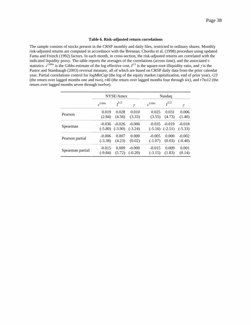
Page 38
Table 6. Risk-adjusted return correlations
The sample consists of stocks present in the CRSP monthly and daily files, restricted to ordinary shares. Monthly risk-adjusted returns are computed in accordance with the Brennan, Chordia et al. (1998) procedure using updated Fama and French (1992) factors. In each month, in cross-section, the risk-adjusted returns are correlated with the indicated liquidity proxy. The table reports the averages of the correlations (across time), and the associated t-statistics. cGibbs is the Gibbs estimate of the log effective cost, I1/2 is the square-root illiquidity ratio, and γ is the Pastor and Stambaugh (2003) reversal measure, all of which are based on CRSP daily data from the prior calendar year. Partial correlations control for logMktCap (the log of the equity market capitalization, end of prior year), r23 (the return over lagged months one and two), r46 (the return over lagged months four through six), and r7to12 (the return over lagged months seven through twelve).
NYSE/Amex Nasdaq
cGibbs I1/2 γ cGibbs I1/2 γ
0.019 0.028 0.010 0.025 0.031 0.006 Pearson (2.84) (4.56) (3.33) (3.55) (4.73) (1.40)
-0.036 -0.026 -0.006 -0.035 -0.019 -0.018 Spearman (-5.80) (-3.90) (-3.24) (-5.16) (-2.51) (-5.33)
-0.006 0.007 0.000 -0.005 0.000 -0.002 Pearson partial (-3.38) (4.23) (0.02) (-1.07) (0.03) (-0.40)
-0.015 0.009 -0.000 -0.015 0.009 0.001 Spearman partial (-9.84) (5.72) (-0.20) (-3.15) (1.83) (0.14)

Page 39
Table 7. Monthly seasonality in the risk-adjusted return correlations
The sample consists of stocks present in the CRSP monthly and daily files, restricted to ordinary shares. Monthly risk-adjusted returns are computed in accordance with the Brennan, Chordia et al. (1998) procedure using updated Fama and French (1992) factors. In each month, in cross-section, the risk-adjusted returns are correlated with the indicated liquidity proxy. The table reports the averages of the correlations (across time), and the associated t-statistics. cGibbs is the Gibbs estimate of the log effective cost, I1/2 is the square-root illiquidity ratio, and γ is the Pastor and Stambaugh (2003) reversal measure, all of which are based on CRSP daily data from the prior calendar year. Partial correlations control for logMktCap (the log of the equity market capitalization, end of prior year), r23 (the return over lagged months one and two), r46 (the return over lagged months four through six), and r7to12 (the return over lagged months seven through twelve).
NYSE/Amex Nasdaq
cGibbs I1/2 γ cGibbs I1/2 γ
0.262 0.245 0.059 0.180 0.150 0.051Pearson (13.49) (13.17) (5.25) (8.97) (7.22) (2.82)
0.187 0.182 0.027 0.106 0.103 0.040Spearman (8.03) (6.82) (4.36) (6.28) (5.11) (5.17)
0.077 -0.008 0.006 0.032 -0.041 -0.002Pearson partial (13.43) (-1.42) (1.21) (1.92) (-2.53) (-0.12)
0.053 -0.027 0.004 0.004 -0.054 -0.004
January
Spearman partial (10.28) (-4.62) (0.86) (0.25) (-3.24) (-0.27)
-0.003 0.008 0.005 0.011 0.020 0.002Pearson (-0.40) (1.47) (1.78) (1.62) (3.14) (0.42)
-0.056 -0.045 -0.009 -0.047 -0.030 -0.023Spearman (-10.22) (-7.29) (-4.91) (-7.28) (-3.91) (-6.88)
-0.013 0.008 -0.000 -0.009 0.004 -0.002Pearson partial (-7.64) (4.92) (-0.32) (-1.71) (0.79) (-0.38)
-0.021 0.013 -0.001 -0.017 0.015 0.001
Non-January
Spearman partial (-13.43) (7.51) (-0.46) (-3.35) (2.82) (0.22)

Page 40
Figure 1. TAQ and CRSP/Gibbs estimates of log effective costs for the Dow Stocks
Log effective cost estimates from TAQ and CRSP (Gibbs). Averages for all NYSE stocks in the Dow index from 1993 to 2003. Vertical lines mark the dates when the NYSE fully implemented sixteenth pricing (July 1, 1997), and decimal pricing (January 29, 2001).

Page 41
Figure 2. Average log effective cost, Gibbs estimates, 1962-2003
Annual averages of Gibbs estimates of log effective cost for all ordinary shares on the CRSP daily file. For both NYSE/Amex and Nasdaq, market capitalization subsamples are defined using NYSE breakpoints.