Trading on Algos*

Johannes A. Skjeltorp�

Norges Bank

Elvira SojliErasmus University Rotterdam

Wing Wah ThamErasmus University Rotterdam and Tinbergen Institute

Preliminary DraftComments welcome

Abstract

This paper studies the impact of algorithmic trading (AT) on asset prices. We findthat the heterogeneity of algorithmic traders across stocks generates predictable patternsin stock returns. A trading strategy that exploits the AT return predictability generatesa monthly risk-adjusted performance between 50-130 basis points for the period 1999to 2012. We find that stocks with lower AT have higher returns, after controlling forstandard market-, size-, book-to-market-, momentum, and liquidity risk factors. Thiseffect survives the inclusion of many cross-sectional return predictors and is statisticallyand economically significant. Return predictability is stronger among stocks with higherimpediments to trade and higher predatory/opportunistic algorithmic traders. Our paperis the first to study and establish a strong link between algorithmic trading and assetprices.

Keywords: Asset pricing, Algorithmic trading, Market quality, Liquidity.

JEL Classification: G10; G20; G14.

*The authors thank Schmuel Baruch, Tarun Chordia, Thierry Foucault, Amit Goyal, Terry Hendershott,Albert Menkveld, Ryan Riordan, Norman Schurhoff, Bernt-Arne Ødegaard, and participants at the NorthernFinance Association Meeting 2013, ESSFM Gerzensee 2013, and the International Workshop on Market Mi-crostructure and Nonlinear Dynamics for useful comments and suggestions. The views expressed are those ofthe authors and should not be interpreted as reflecting those of Norges Bank (Central Bank of Norway).

�Corresponding author. Address: Central Bank of Norway, P.O.Box 1179, Sentrum, NO-0107 Oslo, Nor-way. Email: jsk@nbim.no, Phone: (+47) 22316740. Other authors’ email addresses: esojli@rsm.nl (Sojli),tham@ese.eur.nl (Tham).

1 Introduction

Algorithmic trading (AT) has increased enormously in recent years and it is estimated to

account for 53% of U.S. daily equity trading volume. The episodes of the Flash crash in

2010 and the runaway trading code of Knight Capital in August 2012, which cost $440

million for its shareholders, highlight the economic importance of understanding the impact

of algorithmic trading on asset prices. Despite the growing importance of AT in financial

markets, there is no work studying its impact on asset returns. This paper fills the gap by

examining the cross-sectional relation between AT and stock returns.

A major challenge in studying the impact of AT on market quality and on asset prices

is the availability of long time series of public data. We overcome this issue by constructing

an AT measure based on the order-to-trade ratio (OTR) using (publicly available) Trade

and Quote (TAQ) data and examine its evolution for the period 1999 to 2012.1 Using

detailed high-frequency trading data (hereafter HFT data) obtained from NASDAQ OMX,

we compare our measure with the fraction of trades and quotes by HFT per stock as provided

by NASDAQ.2 This data set is also used by Brogaard, Hendershott, and Riordan (2013) to

study the impact of high-frequency trading on price discovery. We find that our measure is

highly correlated, with a correlation of 65%-75%, to several measures of AT from the HFT

data.

Using a data sample of NYSE, AMEX, and NASDAQ-listed firms from January 1999

to October 2012, we find a raw return differential between the low AT and the high AT

portfolio of 9.4% per year. The AT effect is robust to adjustments for risk factors as well as

firm characteristics. A portfolio of stocks with low AT outperforms a portfolio of stocks with

high AT by 50 to 130 basis points per month after adjusting for the market, size, book-to-

market, momentum, and liquidity factors. The negative relation between AT and returns is

significant even after controlling for other widely documented return predictors. The return

1Hendershott, Jones, and Menkveld (2011) propose the use of message-to-trade ratios as an AT measurefor studying the impact of AT on liquidity in NYSE. SEC Chairman Mary Schapiro supports the use ofOTR as a measure of AT for policies to curb excessive messaging. The European Parliament’s Economic andMonetary Affairs Committee (ECON) suggests to levy a fee for trading members who exceed an OTR of 250:1,see http://www.thetradenews.com/news/Regions/Europe/MEPs_squeeze_HFT_in_MAD_proposals.aspx.

2Hagstromer and Norden (2013) show that 98.2% of HFT messages and 96.7% of their trades are gener-ated using algorithms, while only 13.5% of non-HFT messages and 63.6% of messages from hybrid firms aregenerated by algorithms in the OMXS30 index in 2012.

1

difference is larger among smaller stocks, more illiquid stocks, and stocks with higher delay

in information diffusion. The results are robust to different holding periods and various asset

pricing tests.

We propose two potential explanations for the existence of the AT effect. First, the higher

returns of stocks with low AT may reflect a delay in information diffusion among these stocks.

Biais, Hombert, and Weill (2010) suggest that AT reduces the cognitive inability of human

traders to execute their tasks efficiently and quickly. AT can improve the speed of information

diffusion through trading algorithms that parse information from news wires and electronic

sources almost instantly. More AT represents not only quicker response to news arrivals

and the ability to identify short-lived mis-pricings, but also more information coverage and

aggregation. Thus, more AT decreases delays in information diffusion and reduces trading

frictions, see Chaboud, Chiquoine, Hjalmarsson, and Vega (2009), Hendershott et al. (2011),

and Hendershott and Riordan (2012). Using the Hou and Moskowitz (2005) measure of how

quickly stock prices respond to information, we find little support for the cognitive inability

of human traders hypothesis.

The second explanation is based on the heterogeneity of algorithmic traders across stocks.

The diversity of AT strategies implies a considerable heterogeneity in algorithmic trader

types. In general, AT strategies are classified as market making and predatory algos, and

these different algo types participate in stocks with different characteristics. Hagstromer and

Norden (2013) show that market making algos have higher quote-to-trade ratios and are more

prevalent in smaller stocks with wider tick size, since the profit of market making per trade

increases with the tick size of a stock. However, predatory algos use their speed advantage

over slower traders to respond to news, to anticipate large orders of buy-side institutions, and

to exploit cross-market arbitrage activities. Thus, we expect to find more predatory algos

in stocks with slower traders and with more buy-side institutions. Given the pick-off risk,

slower traders and buy-side institutions will require higher returns.

We test the AT heterogeneity hypothesis using the detailed NASDAQ HFT data with

information on liquidity demanders and suppliers as well as trades between faster algorithms

and slower human traders. We find that risk adjusted returns are higher in stocks with more

active HFT trading against slower passive non-HFT traders and lower for stocks with more

2

market making HFTs. Furthermore, the AT effect is more prevalent in stocks with more

institutional investors. These results suggest that the higher risk-adjusted returns in lower

AT stocks are associated with higher pick-off risk created by opportunistic algos that prefer

to trade with humans and in stocks with more institutional investors.

We also study the role of market frictions/impediments-to-trade on the persistence of the

AT effect. A profitable trading opportunity can persist only if there are market frictions

that discourage arbitrageurs from exploiting it. We find that the AT effect is stronger among

smaller stocks and stocks with higher transaction costs, supporting the impediments-to-trade

hypothesis. Overall, these findings suggest that the AT effect arises from the heterogene-

ity of algorithmic traders across different stocks and impediments-to-trade perpetuate the

phenomenon.

This paper is closely related to the literature on liquidity and asymmetric information

and asset prices. O’Hara (2003) argues that financial markets can play an important role for

asset prices through liquidity and price discovery. Amihud and Mendelson (1986), Brennan

and Subrahmanyam (1996), Brennan, Chordia, and Subrahmanyam (1998), Amihud (2002),

Chordia, Subrahmanyam, and Anshuman (2002b), Jones (2002), and Brennan, Chordia,

Subrahmanyam, and Tong (2012), among many others, provide evidence that liquidity is an

important determinant of expected returns. Brennan and Subrahmanyam (1996), Easley,

Hvidkjaer, and O’Hara (2002) and Easley and O’Hara (2004), among others, argue that

stocks with more information asymmetry should have higher expected returns. We provide

support for these two streams of literature by showing how AT affects asset prices via adverse

selection and stock liquidity levels.

The paper is also related to the growing literature on understanding the impact of al-

gorithmic and high frequency trading in financial markets. Biais and Woolley (2011) and

Jones (2013) provide a survey of the literature on HFT. In theory, algorithmic trading can

be beneficial for financial markets as it may mitigate traders cognition limits (Biais et al.,

2010), but algorithmic traders can increase predatory behavior and adverse selection (Biais,

Foucault, and Moinas, 2011; Foucault, Hombert, and Rosu, 2012) and increase imperfect

competition (Biais et al., 2011). The empirical literature addresses the effects of AT on trade

execution, liquidity, and market efficiency. Algorithms appear to reduce execution costs and

3

risks (Domowitz and Yegerman, 2005; Engle, Ferstenberg, and Russell, 2012) and improve

arbitrageurs’ ability to eliminate asset mispricings (Chaboud et al., 2009). Several papers find

that AT increases competition among trading venues and liquidity providers, provides liq-

uidity when it is scarce, and improves price efficiency (see Hendershott et al., 2011; Chaboud

et al., 2009; Hendershott and Riordan, 2012; Brogaard et al., 2013). However, Kirilenko,

Kyle, Samadi, and Tuzun (2012) provide empirical evidence of adverse selection by showing

that HFT are able to predict price changes at the expense of slower traders. Chaboud et al.

(2009) find more correlated trades among algorithmic traders, which can potentially increase

systemic risk in the spirit of Khandan and Lo (2011). Overall, the evidence on whether mar-

ket quality is higher or lower with AT is mixed. Differently from the existing empirical work

in the market microstructure literature, we investigate the impact of AT on financial markets

through an asset pricing perspective by studying the relation between AT and asset returns

across portfolios with varying algorithmic activity. Our results highlight the importance of

accounting for heterogeneity in algos when studying their impact on market quality and asset

prices.

This paper is among the first to construct a proxy for AT using publicly available data,

which can be used to inform the intense public and academic debate about the impact of AT

on market quality. Previous studies have mainly focused on market microstructure issues due

to the lack of long time series of publicly available data. So far, measures of AT come from

propriety databases and the time series of these measures is short. Chaboud et al. (2009)

study the impact of AT on market efficiency in the foreign exchange market using proprietary

Electronic Broking System (EBS) data from 2003 to 2007. Hendershott et al. (2011) construct

measures of AT using electronic message traffic and trades in NYSE’s SuperDOT system from

the proprietary NYSE’s System Order Data database from 2001 to 2005. Hasbrouck and Saar

(2013) use two months of NASDAQ-ITCH data in 2008 to construct a measure of proprietary

algorithms participation in stocks. Hendershott and Riordan (2012) use proprietary Deutsche

Boerse data which identify whether or not the order was generated with an algorithm for 30

DAX stocks in January 2008. Brogaard et al. (2013) study the role of HFT, a subset of AT,

using NASDAQ data that identifies HFT trading activity on a stratified sample of stocks

(120 stocks) in 2008 and 2009. Boehmer, Fong, and Wu (2012) construct a proxy for AT

4

in 39 individual exchanges around the world from 2001 and 2009 to study the impact of

AT on market quality using the Thomson Reuters Tick History database. Using TAQ data,

we construct an AT measure consistent with Hendershott et al. (2011) and Boehmer et al.

(2012) for the whole U.S. equity market. We validate the reliability of OTR from TAQ as an

appropriate AT measure by comparing it with the shorter but more detailed NASDAQ HFT

data. The validation facilitates future research and analysis on the role and impact of AT in

broader U.S. based asset pricing and corporate finance studies.

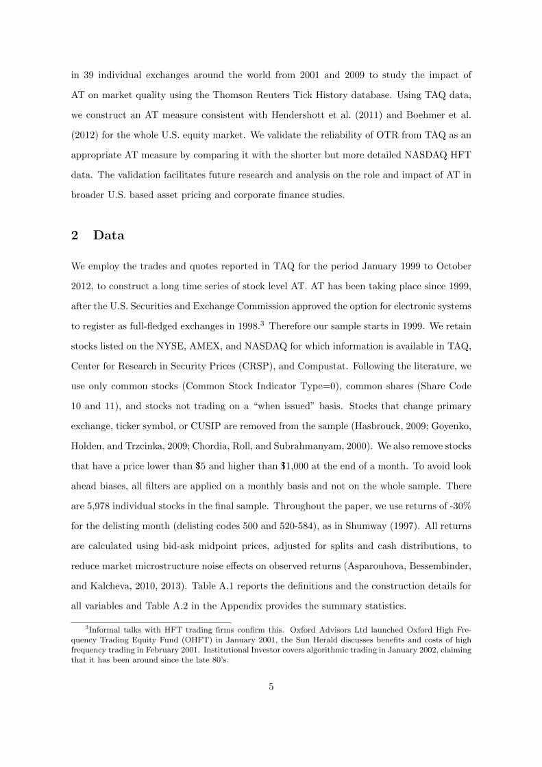
2 Data

We employ the trades and quotes reported in TAQ for the period January 1999 to October

2012, to construct a long time series of stock level AT. AT has been taking place since 1999,

after the U.S. Securities and Exchange Commission approved the option for electronic systems

to register as full-fledged exchanges in 1998.3 Therefore our sample starts in 1999. We retain

stocks listed on the NYSE, AMEX, and NASDAQ for which information is available in TAQ,

Center for Research in Security Prices (CRSP), and Compustat. Following the literature, we

use only common stocks (Common Stock Indicator Type=0), common shares (Share Code

10 and 11), and stocks not trading on a “when issued” basis. Stocks that change primary

exchange, ticker symbol, or CUSIP are removed from the sample (Hasbrouck, 2009; Goyenko,

Holden, and Trzcinka, 2009; Chordia, Roll, and Subrahmanyam, 2000). We also remove stocks

that have a price lower than $5 and higher than $1,000 at the end of a month. To avoid look

ahead biases, all filters are applied on a monthly basis and not on the whole sample. There

are 5,978 individual stocks in the final sample. Throughout the paper, we use returns of -30%

for the delisting month (delisting codes 500 and 520-584), as in Shumway (1997). All returns

are calculated using bid-ask midpoint prices, adjusted for splits and cash distributions, to

reduce market microstructure noise effects on observed returns (Asparouhova, Bessembinder,

and Kalcheva, 2010, 2013). Table A.1 reports the definitions and the construction details for

all variables and Table A.2 in the Appendix provides the summary statistics.

3Informal talks with HFT trading firms confirm this. Oxford Advisors Ltd launched Oxford High Fre-quency Trading Equity Fund (OHFT) in January 2001, the Sun Herald discusses benefits and costs of highfrequency trading in February 2001. Institutional Investor covers algorithmic trading in January 2002, claimingthat it has been around since the late 80’s.

5

2.1 Proxy for algorithmic trading

To investigate the link between AT and asset prices, we need a proxy for stock level AT.

Our proxy is the monthly number of quote updates in TAQ relative to the number of trade

executions (order-to-trade ratio) across all exchanges. We define a quote update as a change

in the best bid or offer price or in the quantity at the best bid/offer price in any exchange. The

order-to-trade ratio has recently been applied by several exchanges to reduce the explosion

of message traffic resulting from the increase in AT.4 As many trading algorithms quote and

cancel orders very rapidly to detect how the market is moving, to trigger responses by other

traders, to identify hidden liquidity, etc., the strategies used by algorithmic traders, and high

frequency traders in particular, have contributed to a huge increase in the amount of message

traffic relative to trade executions. Thus, the order-to-trade ratio should capture changes in

AT both in the cross-section and over time.

We calculate the AT proxy at the monthly frequency for each stock by summing the daily

number of quote updates and the number of trades, across all exchanges. AT for stock i in

month t is measured by the monthly number of messages across all exchanges divided by the

number of trades:

ATi,t =N(quotes)i,tN(trades)i,t

, (1)

where N(quotes)i,t and N(trades)i,t denote the monthly number of quote updates and trades,

respectively, for stock i in month t.5

2.2 Consistency of the AT measure

The AT measure proposed is based on the consideration that the more AT there is, the

more quote updates there will be. Nonetheless, we need to ensure that the measure we

have constructed is reliable and captures AT. We use a set of detailed HFT data obtained

4The London Stock Exchange was the first to introduce an “order management surcharge” in 2005 basedon the number of trades per orders submitted. They revised this charge in 2010. Euronext, which comprisesthe Paris, Amsterdam, Brussels, and Lisbon stock exchanges, has operated one since 2007. In 2012 DirectEdgeintroduced the “Message Efficiency Incentive Program”, where the exchange pays full rebates only to tradersthat have an average monthly message-to-trade ratio less than 100 to 1. In May 2012 the Oslo Stock Exchangeintroduced an order-to-execute fee, where traders that exceed a ratio of 70 for a month incur a charge of NOK0.05 (USD 0.0008) per order. Deutsche Borse and Borsa Italiana have announced similar measures in 2012.

5Another way to measure algorithmic activity is to construct a ratio of trading volume to quote updates,see Hendershott et al. (2011). Our results remain qualitatively the same when using this measure. The resultsare available from the authors upon request.

6

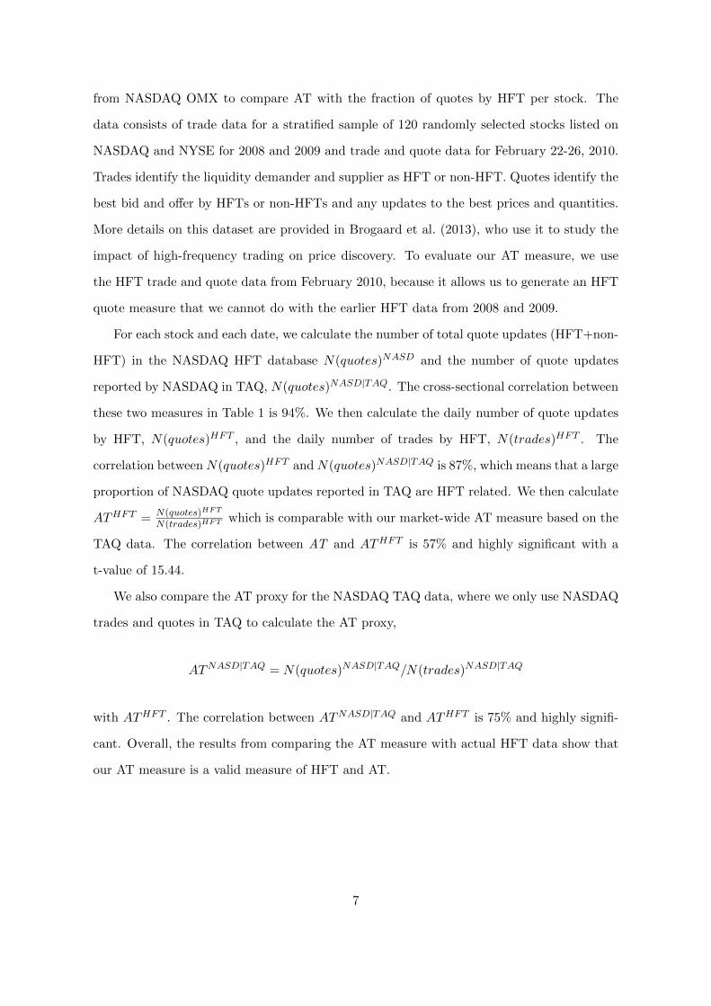
from NASDAQ OMX to compare AT with the fraction of quotes by HFT per stock. The

data consists of trade data for a stratified sample of 120 randomly selected stocks listed on

NASDAQ and NYSE for 2008 and 2009 and trade and quote data for February 22-26, 2010.

Trades identify the liquidity demander and supplier as HFT or non-HFT. Quotes identify the

best bid and offer by HFTs or non-HFTs and any updates to the best prices and quantities.

More details on this dataset are provided in Brogaard et al. (2013), who use it to study the

impact of high-frequency trading on price discovery. To evaluate our AT measure, we use

the HFT trade and quote data from February 2010, because it allows us to generate an HFT

quote measure that we cannot do with the earlier HFT data from 2008 and 2009.

For each stock and each date, we calculate the number of total quote updates (HFT+non-

HFT) in the NASDAQ HFT database N(quotes)NASD and the number of quote updates

reported by NASDAQ in TAQ, N(quotes)NASD|TAQ. The cross-sectional correlation between

these two measures in Table 1 is 94%. We then calculate the daily number of quote updates

by HFT, N(quotes)HFT , and the daily number of trades by HFT, N(trades)HFT . The

correlation betweenN(quotes)HFT andN(quotes)NASD|TAQ is 87%, which means that a large

proportion of NASDAQ quote updates reported in TAQ are HFT related. We then calculate

ATHFT = N(quotes)HFT

N(trades)HFT which is comparable with our market-wide AT measure based on the

TAQ data. The correlation between AT and ATHFT is 57% and highly significant with a

t-value of 15.44.

We also compare the AT proxy for the NASDAQ TAQ data, where we only use NASDAQ

trades and quotes in TAQ to calculate the AT proxy,

ATNASD|TAQ = N(quotes)NASD|TAQ/N(trades)NASD|TAQ

with ATHFT . The correlation between ATNASD|TAQ and ATHFT is 75% and highly signifi-

cant. Overall, the results from comparing the AT measure with actual HFT data show that

our AT measure is a valid measure of HFT and AT.

7

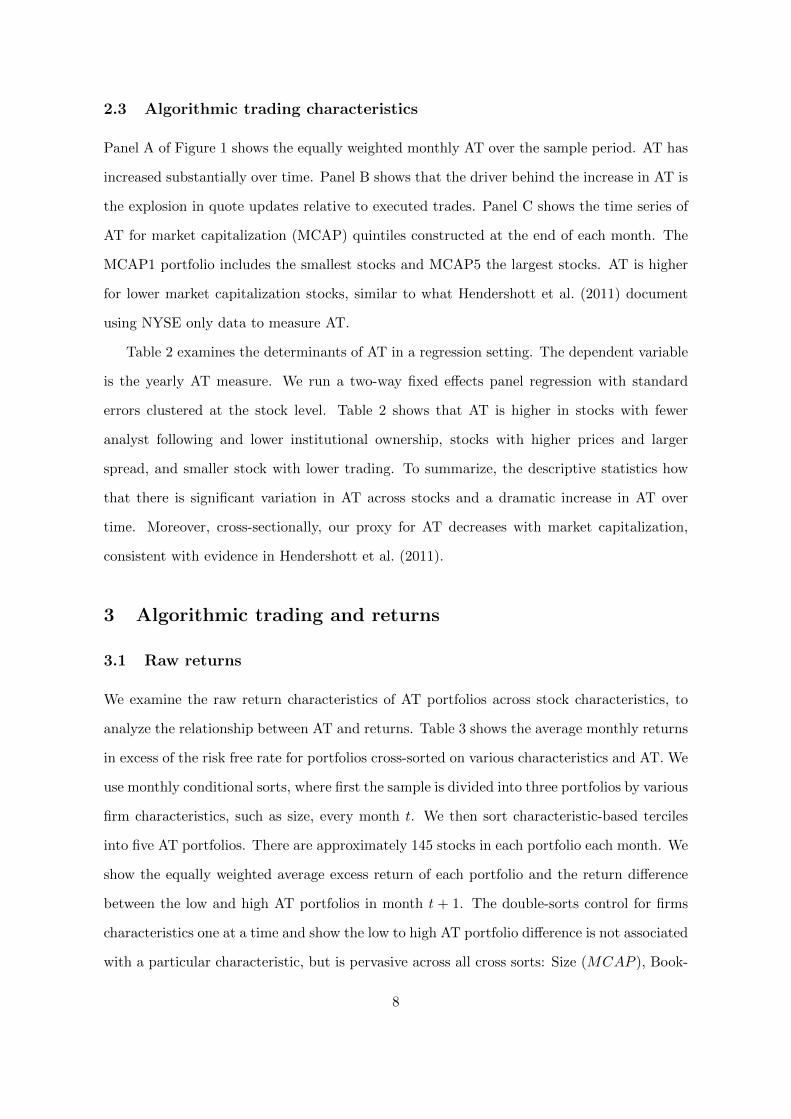
2.3 Algorithmic trading characteristics

Panel A of Figure 1 shows the equally weighted monthly AT over the sample period. AT has

increased substantially over time. Panel B shows that the driver behind the increase in AT is

the explosion in quote updates relative to executed trades. Panel C shows the time series of

AT for market capitalization (MCAP) quintiles constructed at the end of each month. The

MCAP1 portfolio includes the smallest stocks and MCAP5 the largest stocks. AT is higher

for lower market capitalization stocks, similar to what Hendershott et al. (2011) document

using NYSE only data to measure AT.

Table 2 examines the determinants of AT in a regression setting. The dependent variable

is the yearly AT measure. We run a two-way fixed effects panel regression with standard

errors clustered at the stock level. Table 2 shows that AT is higher in stocks with fewer

analyst following and lower institutional ownership, stocks with higher prices and larger

spread, and smaller stock with lower trading. To summarize, the descriptive statistics how

that there is significant variation in AT across stocks and a dramatic increase in AT over

time. Moreover, cross-sectionally, our proxy for AT decreases with market capitalization,

consistent with evidence in Hendershott et al. (2011).

3 Algorithmic trading and returns

3.1 Raw returns

We examine the raw return characteristics of AT portfolios across stock characteristics, to

analyze the relationship between AT and returns. Table 3 shows the average monthly returns

in excess of the risk free rate for portfolios cross-sorted on various characteristics and AT. We

use monthly conditional sorts, where first the sample is divided into three portfolios by various

firm characteristics, such as size, every month t. We then sort characteristic-based terciles

into five AT portfolios. There are approximately 145 stocks in each portfolio each month. We

show the equally weighted average excess return of each portfolio and the return difference

between the low and high AT portfolios in month t + 1. The double-sorts control for firms

characteristics one at a time and show the low to high AT portfolio difference is not associated

with a particular characteristic, but is pervasive across all cross sorts: Size (MCAP ), Book-

8

to-Market (BM), relative spread (SPREAD), USD trading volume (USDV OL), past month

return (R1), and past 12 month return (R212).

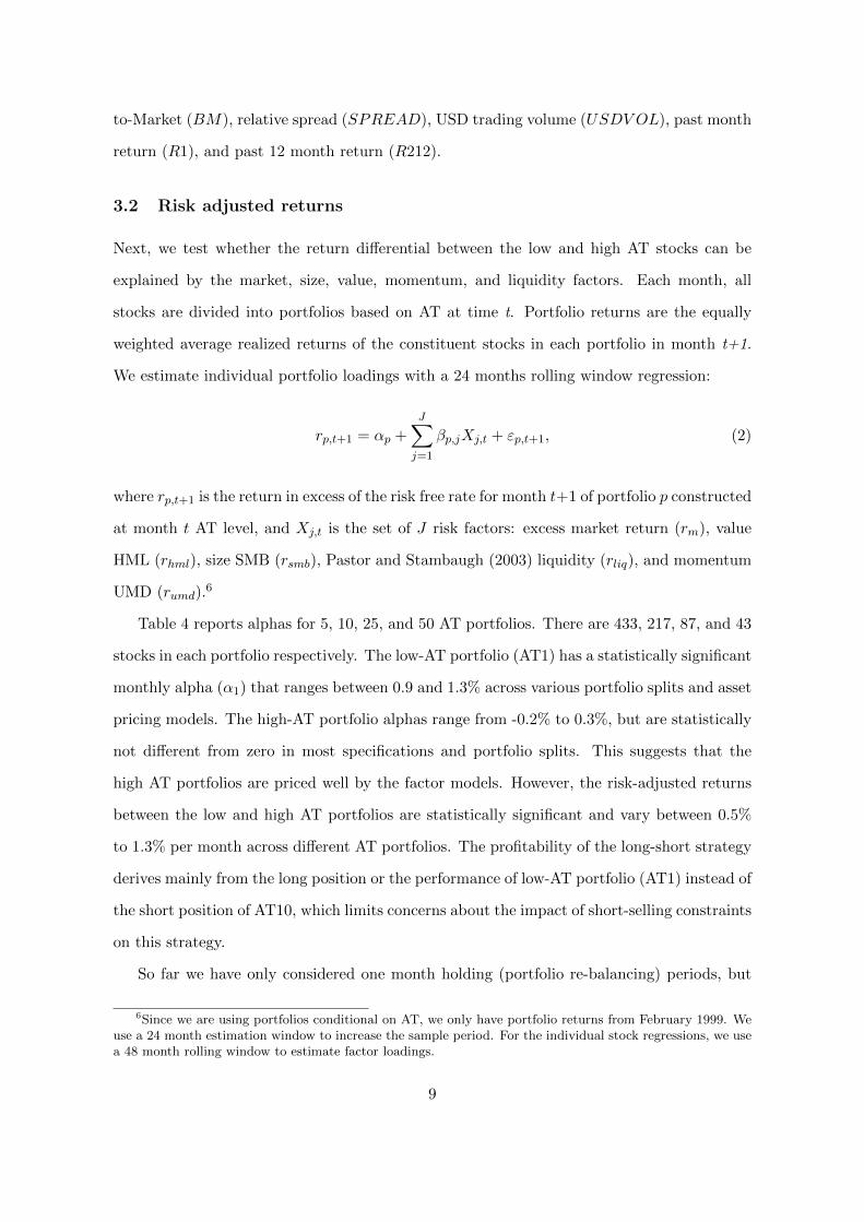
3.2 Risk adjusted returns

Next, we test whether the return differential between the low and high AT stocks can be

explained by the market, size, value, momentum, and liquidity factors. Each month, all

stocks are divided into portfolios based on AT at time t. Portfolio returns are the equally

weighted average realized returns of the constituent stocks in each portfolio in month t+1.

We estimate individual portfolio loadings with a 24 months rolling window regression:

rp,t+1 = αp +J∑j=1

βp,jXj,t + εp,t+1, (2)

where rp,t+1 is the return in excess of the risk free rate for month t+1 of portfolio p constructed

at month t AT level, and Xj,t is the set of J risk factors: excess market return (rm), value

HML (rhml), size SMB (rsmb), Pastor and Stambaugh (2003) liquidity (rliq), and momentum

UMD (rumd).6

Table 4 reports alphas for 5, 10, 25, and 50 AT portfolios. There are 433, 217, 87, and 43

stocks in each portfolio respectively. The low-AT portfolio (AT1) has a statistically significant

monthly alpha (α1) that ranges between 0.9 and 1.3% across various portfolio splits and asset

pricing models. The high-AT portfolio alphas range from -0.2% to 0.3%, but are statistically

not different from zero in most specifications and portfolio splits. This suggests that the

high AT portfolios are priced well by the factor models. However, the risk-adjusted returns

between the low and high AT portfolios are statistically significant and vary between 0.5%

to 1.3% per month across different AT portfolios. The profitability of the long-short strategy

derives mainly from the long position or the performance of low-AT portfolio (AT1) instead of

the short position of AT10, which limits concerns about the impact of short-selling constraints

on this strategy.

So far we have only considered one month holding (portfolio re-balancing) periods, but

6Since we are using portfolios conditional on AT, we only have portfolio returns from February 1999. Weuse a 24 month estimation window to increase the sample period. For the individual stock regressions, we usea 48 month rolling window to estimate factor loadings.

9

the AT effect we document might be a transient phenomenon caused by short-term reversals

and continuations. If the AT effect is temporary, then we expect stocks to switch across

AT portfolios very frequently and the alphas of the AT long-short strategy to vanish over

longer holding periods. To investigate the reversal hypothesis, we examine the persistence of

the AT characteristic in two ways: (1) calculate the average portfolio rank and (2) examine

the average AT in each portfolio. We assign stocks into portfolios based on AT levels at t

and examine the average AT level for these portfolios in month t+k keeping the portfolio

constituents fixed for k months, where k is 1, 3, 6, 12, and 24 months.

Panel A of Table 5 shows the average portfolio rankings, and Panel B shows the average AT

level of the portfolios for different horizons. Both panels suggest that the AT characteristic of

the underlying portfolio stocks is very persistent. While there is some convergence in ranking

and average AT, when increasing the holding horizon, there is still a large and significant

difference in AT ranking and level among the portfolios even at the 24 month horizon. Panel

B shows an increase in the average AT level across portfolios as the horizon increases. This

might be associated with the market-wide increase in the AT activity over the sample period.

We study the average monthly risk adjusted returns (alphas) of the AT long-short strate-

gies for different holding and formation periods, as an alternative exercise, to examine if the

AT effect is transient. Table 6 shows the alphas for strategies that long the low AT portfolio

and short the high AT portfolio for different holding horizons and formation periods. The

holding horizons reflect the number of months for which the portfolio constituents are kept

fixed after the formation point, i.e. portfolios are re-balanced every k months. We construct

the long-short strategies for different numbers of portfolios (5, 10, 25, and 50) and examine

4 different formation periods, i.e. conditioning on different sets of information about AT.

Panel A conditions on AT information from time t, Panels B, C, and D condition on the 3, 6,

and 12-month moving average AT level respectively. We only show alphas from a five factor

model.7 Table 6 shows that the long-short alpha persist for holding horizons up to one year

and is very stable across different portfolios. The AT effect is stronger for 3-12 month holding

periods when conditioning on longer AT information in Panels B to D.

7The results are robust to other factor model specifications and to the creation of more portfolios. Theseresults are available upon request.

10

Figure 2 shows the risk adjusted returns for the high and low AT portfolios for different

holding horizons and formation periods for 5 AT portfolios. Stocks are assigned into portfolios

based on their average AT level over the past 1, 3, 6, and 12 months (formation period) and

the risk adjusted portfolio returns are for holding periods of 1 to 12 months. The figure shows

that the AT effect is very persistent. For the low AT portfolio there is a slightly decreasing

trend as the holding period increases, while the alphas for the high AT portfolios are very

stable across horizons.

The overall conclusion from the above analysis is that AT is a strong predictor of future

abnormal returns (where expected returns are measured by loadings to the three-, four-,

and five-factor models) and this effect is not transient. This finding is consistent with papers

showing that market microstructure and trading activities can be important for understanding

asset returns (Amihud and Mendelson, 1986; Amihud, 2002; Brennan and Subrahmanyam,

1996; Chordia, Roll, and Subrahmanyam, 2002a; Chordia et al., 2000, 2002b; Easley et al.,

2002; Duarte and Young, 2009, among many others).

4 Explaining the algorithmic trading effect

In this section, we investigate and discuss two possible causes for the existence of the AT effect:

cognitive inability of human traders and the diversity of algorithmic traders. In addition, we

study the role of impediments to trade in explaining the persistence of the AT effect.

4.1 Cognitive inability hypothesis

Biais et al. (2010) suggest that AT reduces the cognitive inability of human traders to execute

their tasks efficiently and quickly. For example, trading algorithms parse information from

newswires and electronic sources and use it as trading signals and price adjustments. Thus,

AT can potentially reduce delays in information diffusion. If AT improves information diffu-

sion, then its effect should only be present among stocks with slower speed in incorporating

information.

We employ three measures of how a firm’s stock price responds to information proposed

by Hou and Moskowitz (2005). The market return is used as the relevant news to which

11

stocks respond. Differently from Hou and Moskowitz (2005), we use daily returns instead of

weekly returns, because with recent technological advancements we expect a stock to respond

to changes in market return in days rather than weeks. We run a regression of each stock’s

daily return on contemporaneous and 5 days of lagged returns of the CRSP value-weighted

market portfolio over a year at the end of December:

Ri,t = αi + βiRm,t +5∑

n=1

δ(n)i Rm,t−n + εi,t, (3)

where Ri,t is the return on stock i and Rm,t is the return of CRSP value-weighted portfolio on

day t. βi will be significantly different from zero and all δ(n)i will be statistically insignificant

from zero if the speed of response to market news is immediate. δ(n)i will be significantly

different from zero if the speed of information diffusion is slow.

We use the results of the estimation of Equation 3 to compute three measures. The first

measure is based on an F-test of the joint significance of the lagged variables scaled by the

amount of total variation explained only by Rm,t. This measure is one minus the ratio of the

R2i of the estimation of Equation 3 for each stock with the restriction δ

(n)i = 0 and the R2

i of

the estimation without restrictions:

D1i = 1 −R2

δ(n)i =0,∀n∈[1,5]

R2. (4)

Larger D1 reflects a higher delay in response to new information as more return variation

is captured by the lagged terms. We also use two alternative measures to account for the

precision of the estimates and the lagged specification of the model:

D2i =

∑5n=1 nδ

(n)i

βi +∑5

n=1 δ(n)i

(5)

D3i =

∑5n=1 nδ

(n)i /s.e.(δ

(n)i )

βi/s.e.(βi) +∑5

n=1 δ(n)i /s.e.(δ

(n)i )

, (6)

where s.e. is the standard error of the coefficient estimates.

Table 7 reports monthly alphas of a long-short strategy that longs low AT stocks and short

12

high AT stocks within each level of the delay measure from different factor models. First the

sample is divided into three portfolios by delay measure each month, and then we construct

ten AT portfolios within each tercile. Finally, we long the low AT portfolio and short the

high AT portfolio. For D1, there are abnormal returns in all delay groups, and the highest

returns occur in the high information delay category. Abnormal returns are significant across

all delay groups for D2 and D3. The results suggest that information delay plays some role

in explaining the existence of the AT effect.

As an alternative analysis to investigate the impact of information diffusion on the abnor-

mal returns, we estimate Fama and MacBeth (1973) cross-sectional regressions of monthly

individual stock risk adjusted returns on different firm characteristics including the AT vari-

able. We use individual stocks as test assets to avoid the possibility that tests may be

sensitive to the portfolio grouping procedure. First we estimate monthly rolling regressions

to obtain individual stocks’ risk adjusted returns using a 48 month estimation window. We

use a similar procedure as in Brennan et al. (1998) and Chordia, Subrahmanyam, and Tong

(2011), to first obtain risk adjusted returns eri,t:

eri,t = ri,t −J∑j=1

βi,j,t−1Fj,t, (7)

where ri,t is a stock’s monthly return in excess of the risk free rate, βi,j,t−1 are the factor

loadings estimated for each stock by a rolling time series regression up to t− 1, and Fj,t are

the realized value of the risk factors at t: the market, SMB, HML, liquidity, and momentum.

Then we regress the risk adjusted returns from equation 7 on lagged stock characteristics:

eri,t = c0,t +M∑m=1

cm,tZm,i,t−k + ei,t, (8)

where Zm,i,t−k is the characteristic m for security i at time t−k, and M is the total number of

characteristics. We use k = 1 months for all characteristics.8 The procedure ensures unbiased

estimates of the coefficients, cm,t, without the need to form portfolios, because errors in the

estimation of the factor loadings are included in the dependent variable. The t-statistics are

8Panel A of Table A.4 in the Appendix shows the estimation results where k = 2, except for R1 and R212.

13

obtained using the Fama-Macbeth standard errors with Newey-West correction with 12 lags.

Table 8 reports the Fama and MacBeth (1973) coefficients for different regressions. Col-

umn (1) includes only the AT and delay variables. AT is negative and highly significant

and only D1 is significantly positive at the 10% level. The addition of liquidity variables

in column (2) makes D1 insignificant. AT remains negative and highly significant when we

include all control variables in column (3). These results show little support that the AT ef-

fect is related to the delay in information diffusion and the potential explanation of cognitive

inability hypothesis as discussed in Biais et al. (2010).

4.2 Diversity of algorithmic traders

There is diversity and heterogeneity in the strategies implemented by algorithmic and high

frequency traders. On one hand, HFTs and algorithmic traders can be liquidity providers

or new market makers as documented in Hendershott et al. (2011), Jovanovic and Menkveld

(2010), and Menkveld (2013). Thus, stocks with higher market-making AT should have

better liquidity and lower excess returns. On the other hand, Hagstromer and Norden (2013)

document that there are some HFTs/ATs that follow “opportunitistic” strategies such as

arbitrage, order anticipation, and momentum ignition trading strategies. Such predatory

HFTs/ATs can impose adverse selection costs on other market participants and stocks with

more opportunistic HFTs should have higher excess returns. If the AT effect is related to the

type of algorithmic traders in different portfolios, then the AT variable should be positively

correlated to market making algos and negatively correlated with opportunistic/predatory

algos. Given that predatory algos exploit their speed advantage over other slower traders,

we proxy for predatory algos using the trades initiated (liquidity demanding) by HFT and

liquidity supplied by non-HFT (slower traders) in the NASDAQ HFT data.

We first examine the relation between market making and predatory algos with the AT

variable. Panel A of Table 9 shows the Fama and MacBeth (1973) coefficients from the

monthly contemporaneous regression of AT on HFT type: opportunistic alogs, HFT TAKE,

and market making algos, HFT MAKE. HFT TAKE is the total number of trades (in mil-

lions) for stock i in month t, where an HFT takes liquidity and a non-HFT is a passive party

in the trade. HFT MAKE is the total number of trades, where an HFT provides liquidity

14

(being the passive party in the trade) and the non-HFT take liquidity. We use the NASDAQ

HFT data for 120 stocks for the period 2008 to 2009. Column (1) of Panel A shows that HFT

TAKE is negatively related to AT, while HFT MAKE is positively related to AT. This result

is consistent with Hagstromer and Norden (2013)’s observation that market making HFTs

have higher order-to-trade ratios. The correlation between AT and HFT MAKE and TAKE

suggests that high AT portfolios contain stocks with more market making algos while low AT

portfolios contain stocks with more predatory algos, consistent with the algo heterogeneity

hypothesis. Column (2) excludes HFT MAKE and HFT TAKE and the R2 drops signifi-

cantly, which suggest that HFT explains a significant amount of the cross-sectional variation

in AT.

Following the above observation, we investigate if stocks with more market making HFT

have lower risk-adjusted returns compared to stocks with more predatory HFT. Panel B of

Table 9 shows the Fama-Macbeth regression of the risk adjusted returns from estimating

Equation 8 on HFT MAKE and HFT TAKE. Column (1) shows the result for the full cross

section of stocks (i.e. not limited to the 120 HFT sample stocks) for the period 2008-9. AT

is negative and highly significant in this period. Column (2) replaces the AT variable with

HFT TAKE and HFT MAKE. HFT MAKE has a negative coefficient, similar to AT, while

HFT TAKE is positive and significant. Overall these results support the algo heterogeneity

hypothesis, where stocks with higher risk-adjusted returns are associated with higher amount

of predatory algos and lower amount of market making algos.

Given that order anticipation strategies employed by predatory algos target institutional

investors such as pension and mutual funds, the AT effect should be stronger in stocks with

higher institutional ownership if AT is related to algo heterogeneity. To investigate this, we

examine the abnormal returns of the AT long-short strategy across portfolio with different

percentage of institutional ownership. Stocks are divided into terciles based on the level

of institutional ownership in the previous year. Stocks within each institutional ownership

tercile are divided in 10 AT portfolios, and we compute the alpha of the long-short strategy

based on AT portfolios. Results from Table 10 provide support for the algo heterogeneity

hypothesis. The AT effect is strongest among stocks with the highest institutional owner-

ship. The monthly abnormal returns for portfolios with the highest institutional ownership

15

is 1.7% and 0.65% for the portfolios with the lowest institutional ownership. The difference

in the abnormal returns across different institutional ownership groups is statistically and

economically significant. It appears that predatory algos are more prevalent in stocks with

more institutional investors and returns are higher in these stocks because of pick-off risk.

In summary, the results above suggest that the AT effect is more likely to be driven by

the algo heterogeneity hypothesis and less likely to be explained by the cognitive inability of

human traders hypothesis.

4.3 Impediments to trade effects

Amihud and Mendelson (1986), Brennan and Subrahmanyam (1996), and Hasbrouck (2009)

show that liquidity level plays an important role for the required returns of stocks. Given

algorithms’ role in liquidity provision in today’s financial markets (Menkveld, 2013), the

relation between AT and returns might be due to algorithmic activities proxying for liquidity

levels. Furthermore, the persistence of the AT effect might be caused by impediments to trade

or transaction cost. To determine the role of liquidity and impediments to trade, we first

sort stocks into terciles based on liquidity proxies (ILR, relative spread, and dollar trading

volume), and then create ten AT portfolios within each liquidity tercile. We examine the

alphas from a strategy that long the low AT stocks and short the high AT stocks within each

liquidity tercile. If illiquidity level explains AT, abnormal profits should concentrate in the

most illiquid group and the size of the risk adjusted returns should be of the same magnitude

as the cost of transacting in U.S. equity market. Also abnormal returns for the most illiquid

group should not be statistically different from zero.

Results in Table 11 provide some support for the illiquidity hypothesis. The strongest

AT effect occurs among the most illiquid stocks across all illiquidity proxies. For the five

factor model, the abnormal return for the most illiquid group is about 180 basis points and

70 basis point for the most liquid group across all three illiquidity proxies. The difference in

abnormal returns across these illiquidity groups implies a difference in average transaction

costs (impediment to trade), of 110 basis points between the illiquid and liquid group of

stocks. Most importantly the abnormal returns for the most illiquid group are statistically

and economically different from zero.

16

Table 12 reports the Fama and MacBeth (1973) coefficients for cross-sectional regressions

of individual stock risk adjusted returns on illiquidity variables as in Section 4.1. AT has a

highly significant and negative coefficient, i.e. stocks with higher AT activity have lower next

month risk adjusted returns. We are also interested in the coefficients of the liquidity proxies.

Column (1) includes only SPREAD and AT, column (2) includes only AT and ILR, and

column (3) includes both liquidity proxies. SPREAD and ILR are positive and significant,

and AT remains negative and significant. When including other stock characteristics as

control variables AT continues to be highly significant, while the liquidity variables remain

insignificant.

5 Conclusion

We examine the relation between algorithmic trading and stock returns. We find a significant

risk adjusted return difference between stocks with low and high AT. A trading strategy

that attempts to exploit the AT return predictability generates an annualized risk-adjusted

performance between 7-12% for the period 1999 to 2012. Return predictability is stronger

among stocks with higher impediments to trade and higher information diffusion delay. The

risk adjusted return difference is not only statistically significant but also economically large.

We show that the AT effect is robust to different specifications of asset pricing tests

and well-known return anomalies, and it is not driven by short-term return reversals and

continuations. The AT effect can be explained by the heterogeneity among algorithmic traders

and impediments to trade. Our work contributes to the debate on the role of algorithmic

trading in today’s financial market. It supports the microstructure literature that argues that

AT is in general beneficial for financial markets but only in stocks with higher market making

algorithms. In stocks with more predatory algorithms, we observe higher returns because of

pick-off risk.

17

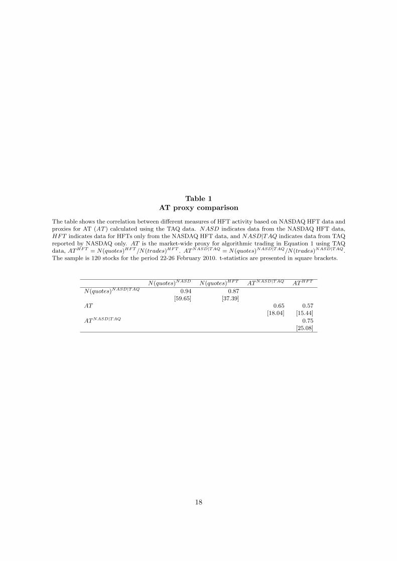
Table 1AT proxy comparison

The table shows the correlation between different measures of HFT activity based on NASDAQ HFT data andproxies for AT (AT ) calculated using the TAQ data. NASD indicates data from the NASDAQ HFT data,HFT indicates data for HFTs only from the NASDAQ HFT data, and NASD|TAQ indicates data from TAQreported by NASDAQ only. AT is the market-wide proxy for algorithmic trading in Equation 1 using TAQdata, ATHFT = N(quotes)HFT /N(trades)HFT . ATNASD|TAQ = N(quotes)NASD|TAQ/N(trades)NASD|TAQ.The sample is 120 stocks for the period 22-26 February 2010. t-statistics are presented in square brackets.

N(quotes)NASD N(quotes)HFT ATNASD|TAQ ATHFT

N(quotes)NASD|TAQ 0.94 0.87[59.65] [37.39]

AT 0.65 0.57[18.04] [15.44]

ATNASD|TAQ 0.75[25.08]

18

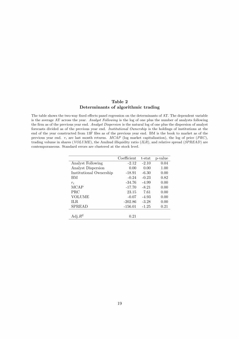
Table 2Determinants of algorithmic trading

The table shows the two-way fixed effects panel regression on the determinants of AT. The dependent variableis the average AT across the year. Analyst Following is the log of one plus the number of analysts followingthe firm as of the previous year end. Analyst Dispersion is the natural log of one plus the dispersion of analystforecasts divided as of the previous year end. Institutional Ownership is the holdings of institutions at theend of the year constructed from 13F files as of the previous year end. BM is the book to market as of theprevious year end. ri are last month returns. MCAP (log market capitalization), the log of price (PRC ),trading volume in shares (VOLUME), the Amihud illiquidity ratio (ILR), and relative spread (SPREAD) arecontemporaneous. Standard errors are clustered at the stock level.

Coefficient t-stat p-valueAnalyst Following -2.12 -2.10 0.04Analyst Dispersion 0.00 0.00 1.00Institutional Ownership -18.91 -6.30 0.00BM -0.24 -0.23 0.82ri -34.76 -4.99 0.00MCAP -17.70 -8.21 0.00PRC 23.15 7.61 0.00VOLUME -0.07 -4.93 0.00ILR -202.86 -3.28 0.00SPREAD -156.01 -1.25 0.21

Adj.R2 0.21

19

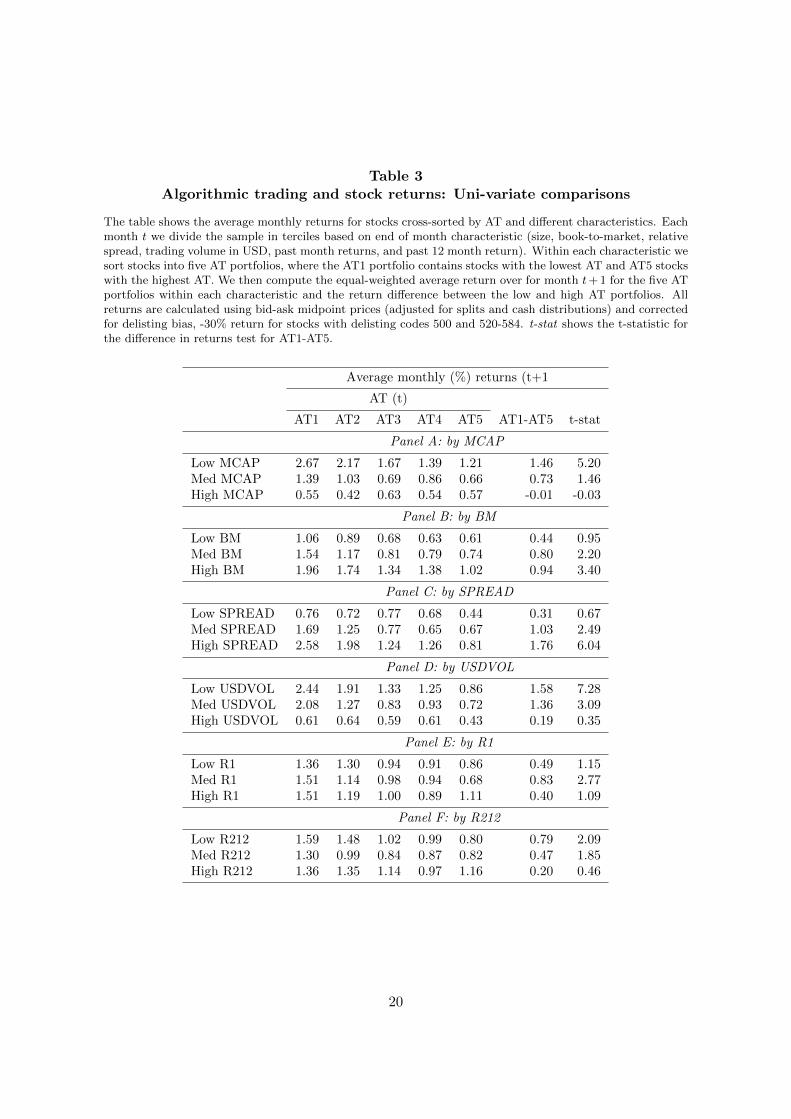
Table 3Algorithmic trading and stock returns: Uni-variate comparisons

The table shows the average monthly returns for stocks cross-sorted by AT and different characteristics. Eachmonth t we divide the sample in terciles based on end of month characteristic (size, book-to-market, relativespread, trading volume in USD, past month returns, and past 12 month return). Within each characteristic wesort stocks into five AT portfolios, where the AT1 portfolio contains stocks with the lowest AT and AT5 stockswith the highest AT. We then compute the equal-weighted average return over for month t+ 1 for the five ATportfolios within each characteristic and the return difference between the low and high AT portfolios. Allreturns are calculated using bid-ask midpoint prices (adjusted for splits and cash distributions) and correctedfor delisting bias, -30% return for stocks with delisting codes 500 and 520-584. t-stat shows the t-statistic forthe difference in returns test for AT1-AT5.

Average monthly (%) returns (t+1

AT (t)

AT1 AT2 AT3 AT4 AT5 AT1-AT5 t-stat

Panel A: by MCAP

Low MCAP 2.67 2.17 1.67 1.39 1.21 1.46 5.20Med MCAP 1.39 1.03 0.69 0.86 0.66 0.73 1.46High MCAP 0.55 0.42 0.63 0.54 0.57 -0.01 -0.03

Panel B: by BM

Low BM 1.06 0.89 0.68 0.63 0.61 0.44 0.95Med BM 1.54 1.17 0.81 0.79 0.74 0.80 2.20High BM 1.96 1.74 1.34 1.38 1.02 0.94 3.40

Panel C: by SPREAD

Low SPREAD 0.76 0.72 0.77 0.68 0.44 0.31 0.67Med SPREAD 1.69 1.25 0.77 0.65 0.67 1.03 2.49High SPREAD 2.58 1.98 1.24 1.26 0.81 1.76 6.04

Panel D: by USDVOL

Low USDVOL 2.44 1.91 1.33 1.25 0.86 1.58 7.28Med USDVOL 2.08 1.27 0.83 0.93 0.72 1.36 3.09High USDVOL 0.61 0.64 0.59 0.61 0.43 0.19 0.35

Panel E: by R1

Low R1 1.36 1.30 0.94 0.91 0.86 0.49 1.15Med R1 1.51 1.14 0.98 0.94 0.68 0.83 2.77High R1 1.51 1.19 1.00 0.89 1.11 0.40 1.09

Panel F: by R212

Low R212 1.59 1.48 1.02 0.99 0.80 0.79 2.09Med R212 1.30 0.99 0.84 0.87 0.82 0.47 1.85High R212 1.36 1.35 1.14 0.97 1.16 0.20 0.46

20

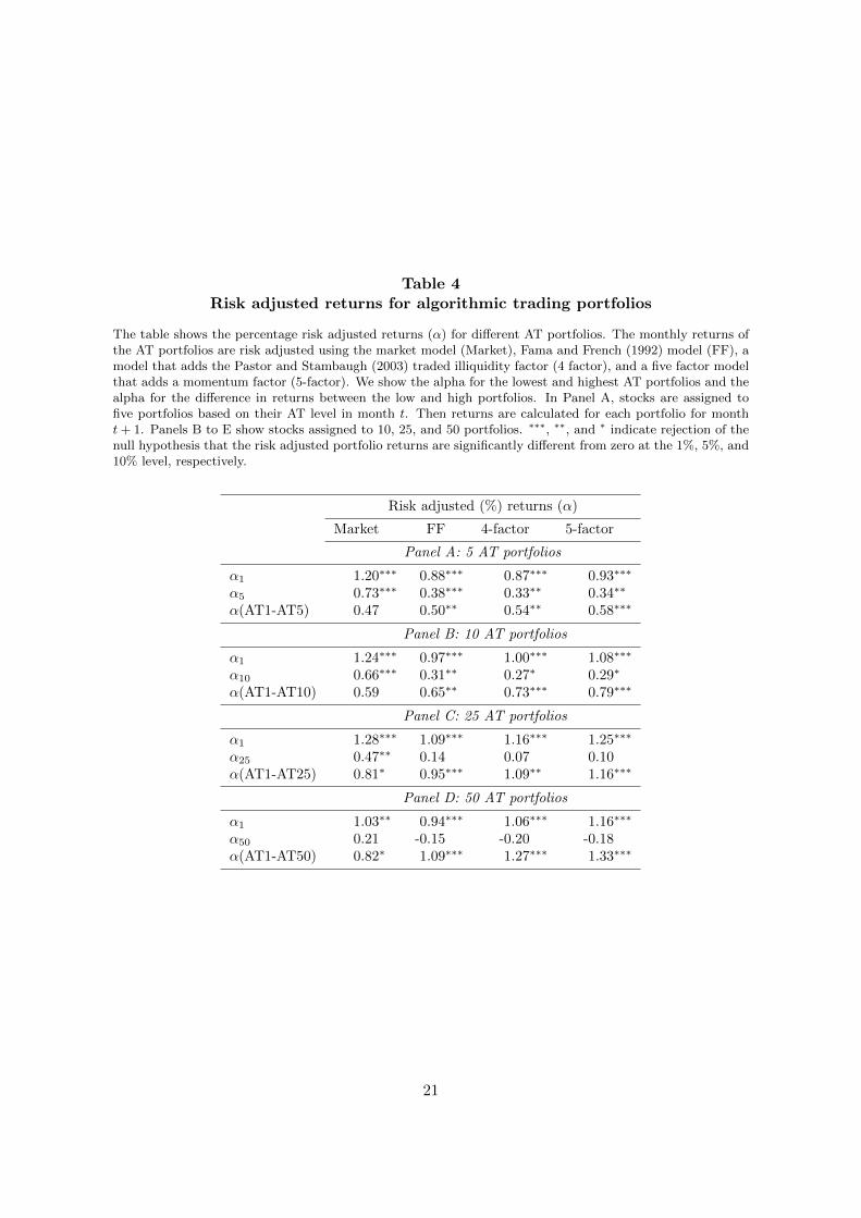
Table 4Risk adjusted returns for algorithmic trading portfolios

The table shows the percentage risk adjusted returns (α) for different AT portfolios. The monthly returns ofthe AT portfolios are risk adjusted using the market model (Market), Fama and French (1992) model (FF), amodel that adds the Pastor and Stambaugh (2003) traded illiquidity factor (4 factor), and a five factor modelthat adds a momentum factor (5-factor). We show the alpha for the lowest and highest AT portfolios and thealpha for the difference in returns between the low and high portfolios. In Panel A, stocks are assigned tofive portfolios based on their AT level in month t. Then returns are calculated for each portfolio for montht+ 1. Panels B to E show stocks assigned to 10, 25, and 50 portfolios. ∗∗∗, ∗∗, and ∗ indicate rejection of thenull hypothesis that the risk adjusted portfolio returns are significantly different from zero at the 1%, 5%, and10% level, respectively.

Risk adjusted (%) returns (α)

Market FF 4-factor 5-factor

Panel A: 5 AT portfolios

α1 1.20∗∗∗ 0.88∗∗∗ 0.87∗∗∗ 0.93∗∗∗

α5 0.73∗∗∗ 0.38∗∗∗ 0.33∗∗ 0.34∗∗

α(AT1-AT5) 0.47 0.50∗∗ 0.54∗∗ 0.58∗∗∗

Panel B: 10 AT portfolios

α1 1.24∗∗∗ 0.97∗∗∗ 1.00∗∗∗ 1.08∗∗∗

α10 0.66∗∗∗ 0.31∗∗ 0.27∗ 0.29∗

α(AT1-AT10) 0.59 0.65∗∗ 0.73∗∗∗ 0.79∗∗∗

Panel C: 25 AT portfolios

α1 1.28∗∗∗ 1.09∗∗∗ 1.16∗∗∗ 1.25∗∗∗

α25 0.47∗∗ 0.14 0.07 0.10α(AT1-AT25) 0.81∗ 0.95∗∗∗ 1.09∗∗ 1.16∗∗∗

Panel D: 50 AT portfolios

α1 1.03∗∗ 0.94∗∗∗ 1.06∗∗∗ 1.16∗∗∗

α50 0.21 -0.15 -0.20 -0.18α(AT1-AT50) 0.82∗ 1.09∗∗∗ 1.27∗∗∗ 1.33∗∗∗

21

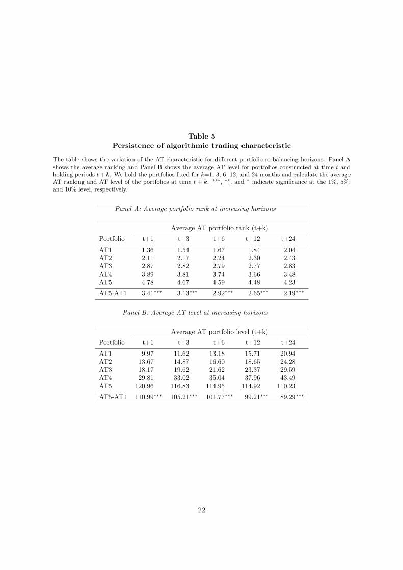
Table 5Persistence of algorithmic trading characteristic

The table shows the variation of the AT characteristic for different portfolio re-balancing horizons. Panel Ashows the average ranking and Panel B shows the average AT level for portfolios constructed at time t andholding periods t+ k. We hold the portfolios fixed for k=1, 3, 6, 12, and 24 months and calculate the averageAT ranking and AT level of the portfolios at time t + k. ∗∗∗, ∗∗, and ∗ indicate significance at the 1%, 5%,and 10% level, respectively.

Panel A: Average portfolio rank at increasing horizons

Average AT portfolio rank (t+k)

Portfolio t+1 t+3 t+6 t+12 t+24

AT1 1.36 1.54 1.67 1.84 2.04AT2 2.11 2.17 2.24 2.30 2.43AT3 2.87 2.82 2.79 2.77 2.83AT4 3.89 3.81 3.74 3.66 3.48AT5 4.78 4.67 4.59 4.48 4.23

AT5-AT1 3.41∗∗∗ 3.13∗∗∗ 2.92∗∗∗ 2.65∗∗∗ 2.19∗∗∗

Panel B: Average AT level at increasing horizons

Average AT portfolio level (t+k)

Portfolio t+1 t+3 t+6 t+12 t+24

AT1 9.97 11.62 13.18 15.71 20.94AT2 13.67 14.87 16.60 18.65 24.28AT3 18.17 19.62 21.62 23.37 29.59AT4 29.81 33.02 35.04 37.96 43.49AT5 120.96 116.83 114.95 114.92 110.23

AT5-AT1 110.99∗∗∗ 105.21∗∗∗ 101.77∗∗∗ 99.21∗∗∗ 89.29∗∗∗

22

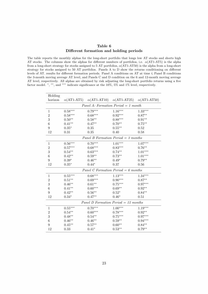
Table 6Different formation and holding periods

The table reports the monthly alphas for the long-short portfolio that longs low AT stocks and shorts highAT stocks. The columns show the alphas for different numbers of portfolios, i.e. α(AT1-AT5) is the alphafrom a long-short strategy for stocks assigned to 5 AT portfolios, α(AT1-AT50) is the alpha from a long-shortstrategy for stocks assigned to 50 AT portfolios. Panels A to D show the returns conditioning on differentlevels of AT. results for different formation periods. Panel A conditions on AT at time t, Panel B conditionsthe 3-month moving average AT level, and Panels C and D condition on the 6 and 12-month moving averageAT level, respectively. All alphas are obtained by risk adjusting the long-short portfolio returns using a fivefactor model. ∗, ∗∗, and ∗∗∗ indicate significance at the 10%, 5% and 1% level, respectively.

Holdinghorizon α(AT1-AT5) α(AT1-AT10) α(AT1-AT25) α(AT1-AT50)

Panel A: Formation Period = 1 month

1 0.58∗∗∗ 0.79∗∗∗ 1.16∗∗∗ 1.33∗∗∗

2 0.58∗∗∗ 0.68∗∗∗ 0.92∗∗∗ 0.87∗∗

3 0.50∗∗ 0.58∗∗ 0.88∗∗∗ 0.91∗∗

6 0.41∗∗ 0.47∗∗ 0.70∗∗ 0.75∗∗

9 0.35∗ 0.35 0.55∗∗ 0.5212 0.31 0.35 0.40 0.58

Panel B Formation Period = 3 months

1 0.56∗∗∗ 0.70∗∗∗ 1.01∗∗∗ 1.07∗∗∗

2 0.57∗∗∗ 0.68∗∗∗ 0.83∗∗∗ 0.76∗∗

3 0.54∗∗ 0.63∗∗∗ 0.74∗∗ 1.01∗∗∗

6 0.42∗∗ 0.59∗∗ 0.73∗∗ 1.01∗∗∗

9 0.39∗ 0.46∗∗ 0.49∗ 0.79∗∗

12 0.35∗ 0.44∗ 0.37 0.56

Panel C Formation Period = 6 months

1 0.55∗∗∗ 0.68∗∗∗ 1.13∗∗∗ 1.34∗∗∗

2 0.51∗∗ 0.69∗∗∗ 0.90∗∗∗ 0.87∗∗

3 0.46∗∗ 0.61∗∗ 0.75∗∗∗ 0.97∗∗∗

6 0.41∗∗ 0.60∗∗∗ 0.69∗∗ 0.92∗∗

9 0.42∗∗ 0.56∗∗ 0.52∗ 0.84∗∗

12 0.34∗ 0.47∗∗ 0.46∗ 0.51

Panel D Formation Period = 12 months

1 0.55∗∗∗ 0.70∗∗∗ 1.00∗∗∗ 1.19∗∗∗

2 0.54∗∗ 0.60∗∗∗ 0.78∗∗∗ 0.92∗∗

3 0.48∗∗ 0.54∗∗ 0.75∗∗∗ 0.97∗∗∗

6 0.46∗∗ 0.46∗∗ 0.59∗∗ 0.94∗∗∗

9 0.45∗∗ 0.57∗∗ 0.60∗∗ 0.84∗∗

12 0.33 0.41∗ 0.53∗∗ 0.79∗∗

23

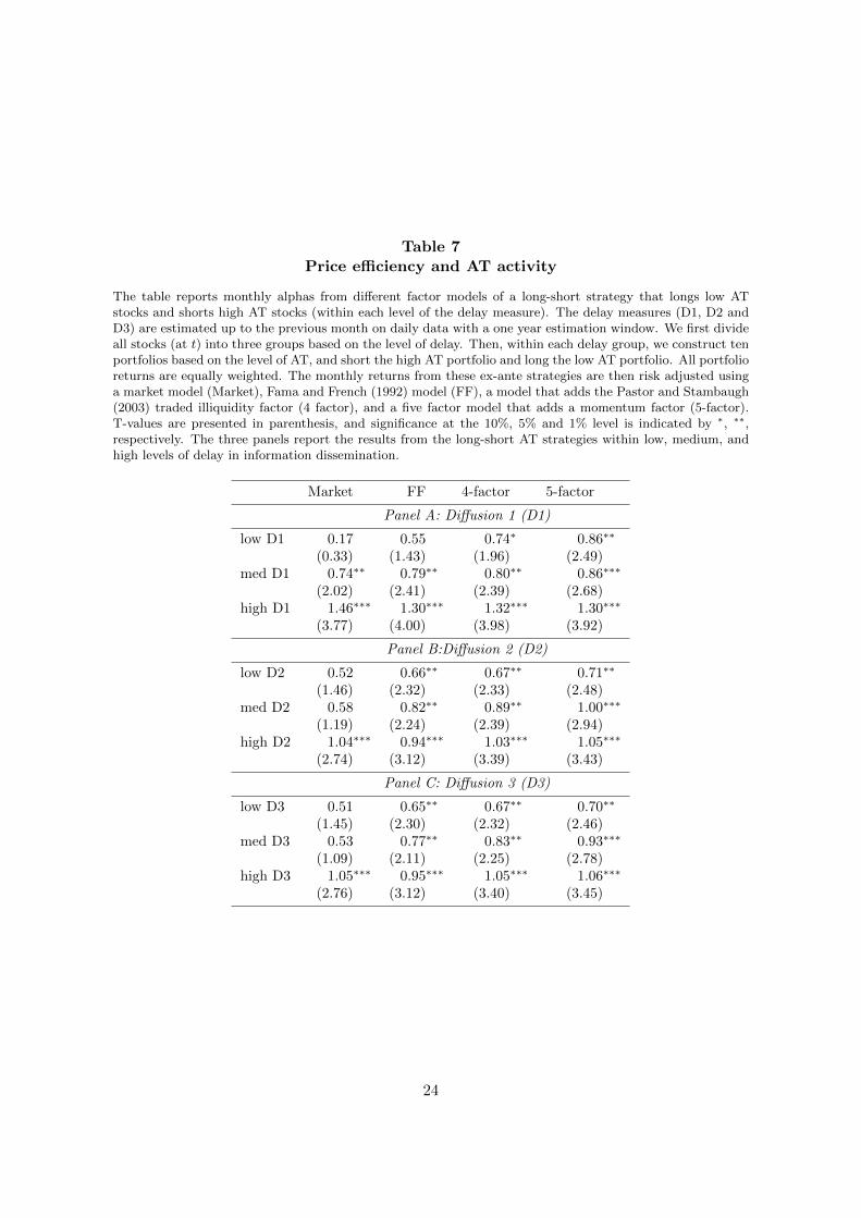
Table 7Price efficiency and AT activity

The table reports monthly alphas from different factor models of a long-short strategy that longs low ATstocks and shorts high AT stocks (within each level of the delay measure). The delay measures (D1, D2 andD3) are estimated up to the previous month on daily data with a one year estimation window. We first divideall stocks (at t) into three groups based on the level of delay. Then, within each delay group, we construct tenportfolios based on the level of AT, and short the high AT portfolio and long the low AT portfolio. All portfolioreturns are equally weighted. The monthly returns from these ex-ante strategies are then risk adjusted usinga market model (Market), Fama and French (1992) model (FF), a model that adds the Pastor and Stambaugh(2003) traded illiquidity factor (4 factor), and a five factor model that adds a momentum factor (5-factor).T-values are presented in parenthesis, and significance at the 10%, 5% and 1% level is indicated by ∗, ∗∗,respectively. The three panels report the results from the long-short AT strategies within low, medium, andhigh levels of delay in information dissemination.

Market FF 4-factor 5-factor

Panel A: Diffusion 1 (D1)

low D1 0.17 0.55 0.74∗ 0.86∗∗

(0.33) (1.43) (1.96) (2.49)med D1 0.74∗∗ 0.79∗∗ 0.80∗∗ 0.86∗∗∗

(2.02) (2.41) (2.39) (2.68)high D1 1.46∗∗∗ 1.30∗∗∗ 1.32∗∗∗ 1.30∗∗∗

(3.77) (4.00) (3.98) (3.92)

Panel B:Diffusion 2 (D2)

low D2 0.52 0.66∗∗ 0.67∗∗ 0.71∗∗

(1.46) (2.32) (2.33) (2.48)med D2 0.58 0.82∗∗ 0.89∗∗ 1.00∗∗∗

(1.19) (2.24) (2.39) (2.94)high D2 1.04∗∗∗ 0.94∗∗∗ 1.03∗∗∗ 1.05∗∗∗

(2.74) (3.12) (3.39) (3.43)

Panel C: Diffusion 3 (D3)

low D3 0.51 0.65∗∗ 0.67∗∗ 0.70∗∗

(1.45) (2.30) (2.32) (2.46)med D3 0.53 0.77∗∗ 0.83∗∗ 0.93∗∗∗

(1.09) (2.11) (2.25) (2.78)high D3 1.05∗∗∗ 0.95∗∗∗ 1.05∗∗∗ 1.06∗∗∗

(2.76) (3.12) (3.40) (3.45)

24

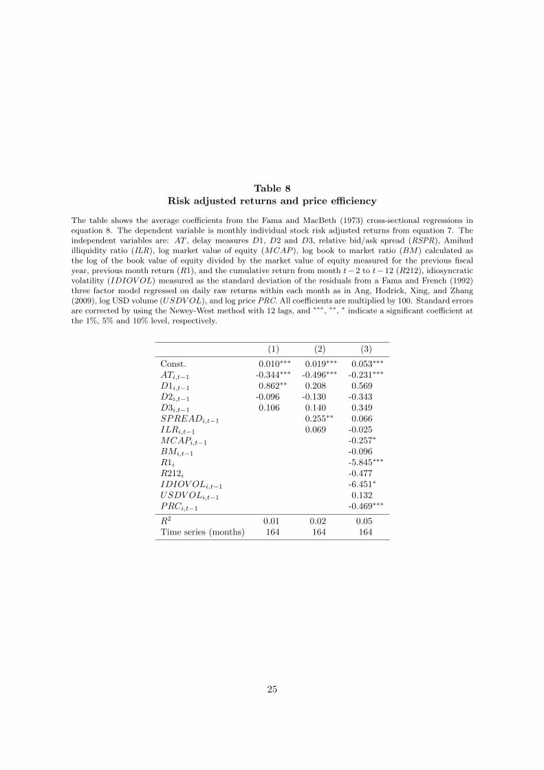
Table 8Risk adjusted returns and price efficiency

The table shows the average coefficients from the Fama and MacBeth (1973) cross-sectional regressions inequation 8. The dependent variable is monthly individual stock risk adjusted returns from equation 7. Theindependent variables are: AT , delay measures D1, D2 and D3, relative bid/ask spread (RSPR), Amihudilliquidity ratio (ILR), log market value of equity (MCAP ), log book to market ratio (BM) calculated asthe log of the book value of equity divided by the market value of equity measured for the previous fiscalyear, previous month return (R1), and the cumulative return from month t− 2 to t− 12 (R212), idiosyncraticvolatility (IDIOV OL) measured as the standard deviation of the residuals from a Fama and French (1992)three factor model regressed on daily raw returns within each month as in Ang, Hodrick, Xing, and Zhang(2009), log USD volume (USDV OL), and log price PRC. All coefficients are multiplied by 100. Standard errorsare corrected by using the Newey-West method with 12 lags, and ∗∗∗, ∗∗, ∗ indicate a significant coefficient atthe 1%, 5% and 10% level, respectively.

(1) (2) (3)

Const. 0.010∗∗∗ 0.019∗∗∗ 0.053∗∗∗

ATi,t−1 -0.344∗∗∗ -0.496∗∗∗ -0.231∗∗∗

D1i,t−1 0.862∗∗ 0.208 0.569D2i,t−1 -0.096 -0.130 -0.343D3i,t−1 0.106 0.140 0.349SPREADi,t−1 0.255∗∗ 0.066ILRi,t−1 0.069 -0.025MCAPi,t−1 -0.257∗

BMi,t−1 -0.096R1i -5.845∗∗∗

R212i -0.477IDIOV OLi,t−1 -6.451∗

USDV OLi,t−1 0.132PRCi,t−1 -0.469∗∗∗

R2 0.01 0.02 0.05Time series (months) 164 164 164

25

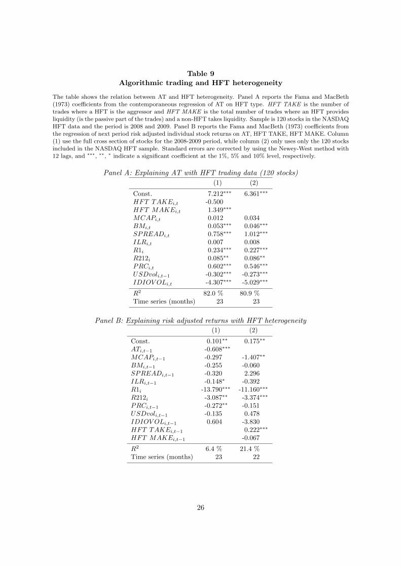
Table 9Algorithmic trading and HFT heterogeneity

The table shows the relation between AT and HFT heterogeneity. Panel A reports the Fama and MacBeth(1973) coefficients from the contemporaneous regression of AT on HFT type. HFT TAKE is the number oftrades where a HFT is the aggressor and HFT MAKE is the total number of trades where an HFT providesliquidity (is the passive part of the trades) and a non-HFT takes liquidity. Sample is 120 stocks in the NASDAQHFT data and the period is 2008 and 2009. Panel B reports the Fama and MacBeth (1973) coefficients fromthe regression of next period risk adjusted individual stock returns on AT, HFT TAKE, HFT MAKE. Column(1) use the full cross section of stocks for the 2008-2009 period, while column (2) only uses only the 120 stocksincluded in the NASDAQ HFT sample. Standard errors are corrected by using the Newey-West method with12 lags, and ∗∗∗, ∗∗, ∗ indicate a significant coefficient at the 1%, 5% and 10% level, respectively.

Panel A: Explaining AT with HFT trading data (120 stocks)

(1) (2)

Const. 7.212∗∗∗ 6.361∗∗∗

HFT TAKEi,t -0.500HFT MAKEi,t 1.349∗∗∗

MCAPi,t 0.012 0.034BMi,t 0.053∗∗∗ 0.046∗∗∗

SPREADi,t 0.758∗∗∗ 1.012∗∗∗

ILRi,t 0.007 0.008R1i 0.234∗∗∗ 0.227∗∗∗

R212i 0.085∗∗ 0.086∗∗

PRCi,t 0.602∗∗∗ 0.546∗∗∗

USDvoli,t−1 -0.302∗∗∗ -0.273∗∗∗

IDIOV OLi,t -4.307∗∗∗ -5.029∗∗∗

R2 82.0 % 80.9 %Time series (months) 23 23

Panel B: Explaining risk adjusted returns with HFT heterogeneity

(1) (2)

Const. 0.101∗∗ 0.175∗∗

ATi,t−1 -0.608∗∗∗

MCAPi,t−1 -0.297 -1.407∗∗

BMi,t−1 -0.255 -0.060SPREADi,t−1 -0.320 2.296ILRi,t−1 -0.148∗ -0.392R1i -13.790∗∗∗ -11.160∗∗∗

R212i -3.087∗∗ -3.374∗∗∗

PRCi,t−1 -0.272∗∗ -0.151USDvoli,t−1 -0.135 0.478IDIOV OLi,t−1 0.604 -3.830HFT TAKEi,t−1 0.222∗∗∗

HFT MAKEi,t−1 -0.067

R2 6.4 % 21.4 %Time series (months) 23 22

26

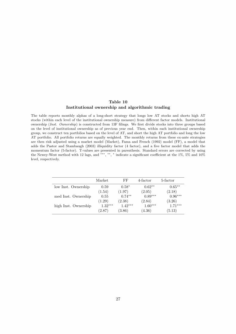
Table 10Institutional ownership and algorithmic trading

The table reports monthly alphas of a long-short strategy that longs low AT stocks and shorts high ATstocks (within each level of the institutional ownership measure) from different factor models. Institutionalownership (Inst. Ownership) is constructed from 13F filings. We first divide stocks into three groups basedon the level of institutional ownership as of previous year end. Then, within each institutional ownershipgroup, we construct ten portfolios based on the level of AT, and short the high AT portfolio and long the lowAT portfolio. All portfolio returns are equally weighted. The monthly returns from these ex-ante strategiesare then risk adjusted using a market model (Market), Fama and French (1992) model (FF), a model thatadds the Pastor and Stambaugh (2003) illiquidity factor (4 factor), and a five factor model that adds themomentum factor (5-factor). T-values are presented in parenthesis. Standard errors are corrected by usingthe Newey-West method with 12 lags, and ∗∗∗, ∗∗, ∗ indicate a significant coefficient at the 1%, 5% and 10%level, respectively.

Market FF 4-factor 5-factor

low Inst. Ownership 0.59 0.58∗ 0.62∗∗ 0.65∗∗

(1.54) (1.97) (2.05) (2.18)med Inst. Ownership 0.55 0.74∗∗ 0.89∗∗∗ 0.96∗∗∗

(1.29) (2.38) (2.84) (3.26)high Inst. Ownership 1.32∗∗∗ 1.42∗∗∗ 1.60∗∗∗ 1.71∗∗∗

(2.87) (3.86) (4.36) (5.13)

27

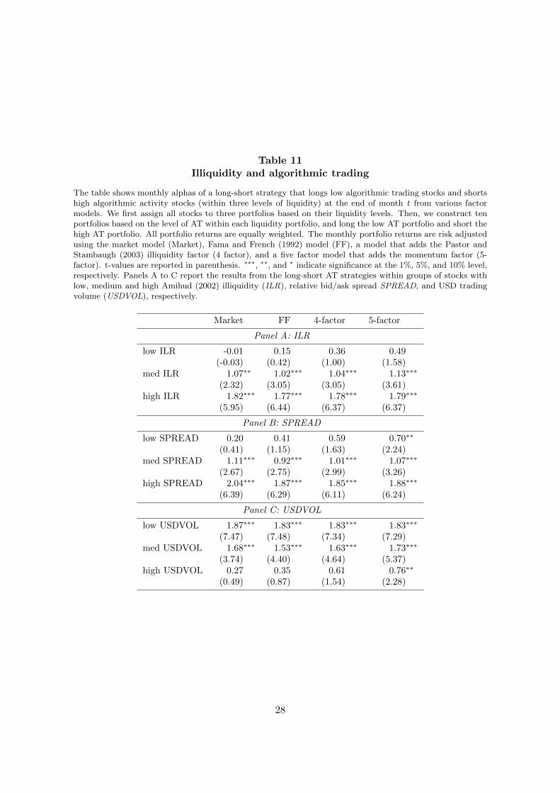
Table 11Illiquidity and algorithmic trading

The table shows monthly alphas of a long-short strategy that longs low algorithmic trading stocks and shortshigh algorithmic activity stocks (within three levels of liquidity) at the end of month t from various factormodels. We first assign all stocks to three portfolios based on their liquidity levels. Then, we construct tenportfolios based on the level of AT within each liquidity portfolio, and long the low AT portfolio and short thehigh AT portfolio. All portfolio returns are equally weighted. The monthly portfolio returns are risk adjustedusing the market model (Market), Fama and French (1992) model (FF), a model that adds the Pastor andStambaugh (2003) illiquidity factor (4 factor), and a five factor model that adds the momentum factor (5-factor). t-values are reported in parenthesis. ∗∗∗, ∗∗, and ∗ indicate significance at the 1%, 5%, and 10% level,respectively. Panels A to C report the results from the long-short AT strategies within groups of stocks withlow, medium and high Amihud (2002) illiquidity (ILR), relative bid/ask spread SPREAD, and USD tradingvolume (USDVOL), respectively.

Market FF 4-factor 5-factor

Panel A: ILR

low ILR -0.01 0.15 0.36 0.49(-0.03) (0.42) (1.00) (1.58)

med ILR 1.07∗∗ 1.02∗∗∗ 1.04∗∗∗ 1.13∗∗∗

(2.32) (3.05) (3.05) (3.61)high ILR 1.82∗∗∗ 1.77∗∗∗ 1.78∗∗∗ 1.79∗∗∗

(5.95) (6.44) (6.37) (6.37)

Panel B: SPREAD

low SPREAD 0.20 0.41 0.59 0.70∗∗

(0.41) (1.15) (1.63) (2.24)med SPREAD 1.11∗∗∗ 0.92∗∗∗ 1.01∗∗∗ 1.07∗∗∗

(2.67) (2.75) (2.99) (3.26)high SPREAD 2.04∗∗∗ 1.87∗∗∗ 1.85∗∗∗ 1.88∗∗∗

(6.39) (6.29) (6.11) (6.24)

Panel C: USDVOL

low USDVOL 1.87∗∗∗ 1.83∗∗∗ 1.83∗∗∗ 1.83∗∗∗

(7.47) (7.48) (7.34) (7.29)med USDVOL 1.68∗∗∗ 1.53∗∗∗ 1.63∗∗∗ 1.73∗∗∗

(3.74) (4.40) (4.64) (5.37)high USDVOL 0.27 0.35 0.61 0.76∗∗

(0.49) (0.87) (1.54) (2.28)

28

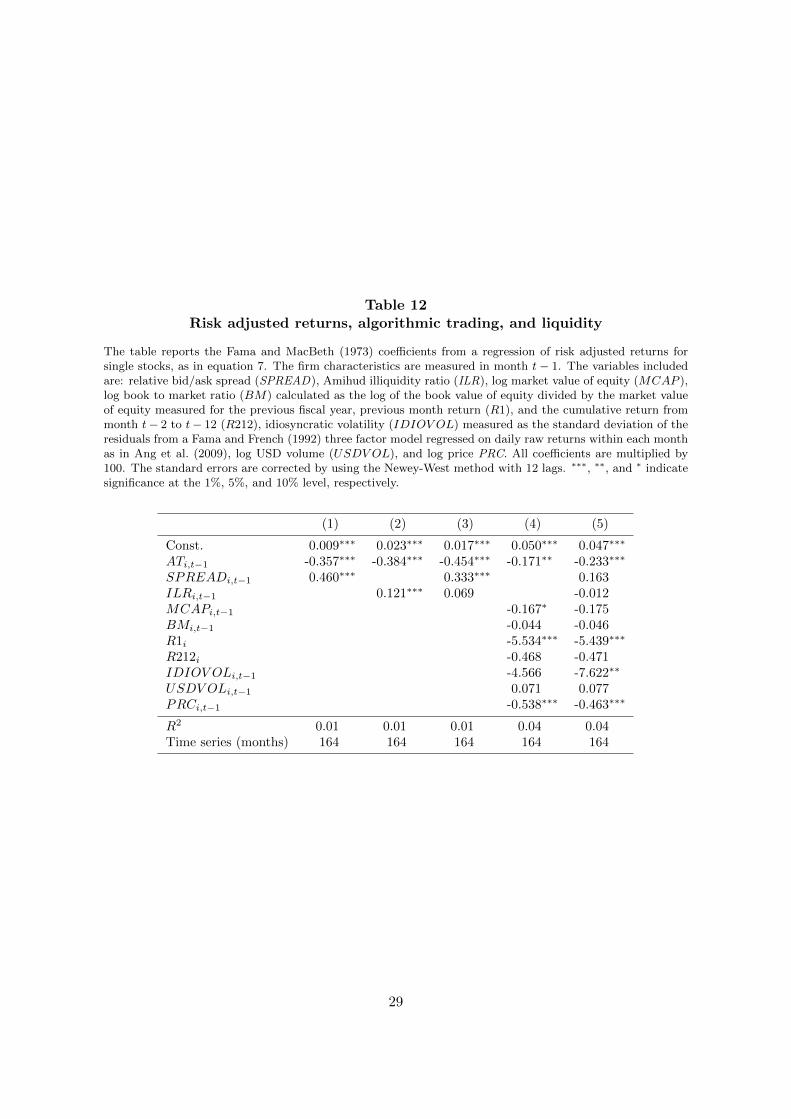
Table 12Risk adjusted returns, algorithmic trading, and liquidity

The table reports the Fama and MacBeth (1973) coefficients from a regression of risk adjusted returns forsingle stocks, as in equation 7. The firm characteristics are measured in month t− 1. The variables includedare: relative bid/ask spread (SPREAD), Amihud illiquidity ratio (ILR), log market value of equity (MCAP ),log book to market ratio (BM) calculated as the log of the book value of equity divided by the market valueof equity measured for the previous fiscal year, previous month return (R1), and the cumulative return frommonth t− 2 to t− 12 (R212), idiosyncratic volatility (IDIOV OL) measured as the standard deviation of theresiduals from a Fama and French (1992) three factor model regressed on daily raw returns within each monthas in Ang et al. (2009), log USD volume (USDV OL), and log price PRC. All coefficients are multiplied by100. The standard errors are corrected by using the Newey-West method with 12 lags. ∗∗∗, ∗∗, and ∗ indicatesignificance at the 1%, 5%, and 10% level, respectively.

(1) (2) (3) (4) (5)

Const. 0.009∗∗∗ 0.023∗∗∗ 0.017∗∗∗ 0.050∗∗∗ 0.047∗∗∗

ATi,t−1 -0.357∗∗∗ -0.384∗∗∗ -0.454∗∗∗ -0.171∗∗ -0.233∗∗∗

SPREADi,t−1 0.460∗∗∗ 0.333∗∗∗ 0.163ILRi,t−1 0.121∗∗∗ 0.069 -0.012MCAPi,t−1 -0.167∗ -0.175BMi,t−1 -0.044 -0.046R1i -5.534∗∗∗ -5.439∗∗∗

R212i -0.468 -0.471IDIOV OLi,t−1 -4.566 -7.622∗∗

USDV OLi,t−1 0.071 0.077PRCi,t−1 -0.538∗∗∗ -0.463∗∗∗

R2 0.01 0.01 0.01 0.04 0.04Time series (months) 164 164 164 164 164

29

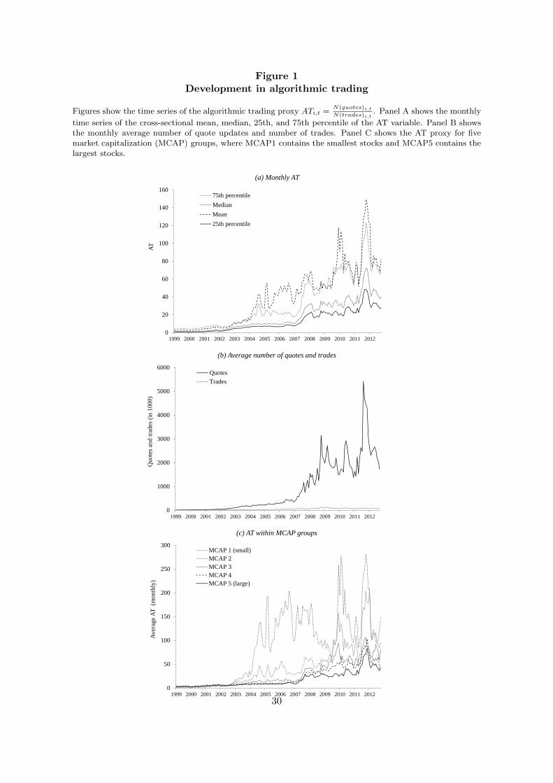
Figure 1Development in algorithmic trading

Figures show the time series of the algorithmic trading proxy ATi,t =N(quotes)i,tN(trades)i,t

. Panel A shows the monthly

time series of the cross-sectional mean, median, 25th, and 75th percentile of the AT variable. Panel B showsthe monthly average number of quote updates and number of trades. Panel C shows the AT proxy for fivemarket capitalization (MCAP) groups, where MCAP1 contains the smallest stocks and MCAP5 contains thelargest stocks.

0

20

40

60

80

100

120

140

160

1999 2000 2001 2002 2003 2004 2005 2006 2007 2008 2009 2010 2011 2012

AT

(a) Monthly AT

75th percentileMedianMean25th percentile

0

1000

2000

3000

4000

5000

6000

1999 2000 2001 2002 2003 2004 2005 2006 2007 2008 2009 2010 2011 2012

Quo

tes a

nd tr

ades

(in

1000

)

(b) Average number of quotes and trades

QuotesTrades

0

50

100

150

200

250

300

1999 2000 2001 2002 2003 2004 2005 2006 2007 2008 2009 2010 2011 2012

Aver

age A

T (m

onth

ly)

(c) AT within MCAP groups

MCAP 1 (small)MCAP 2MCAP 3MCAP 4MCAP 5 (large)

30

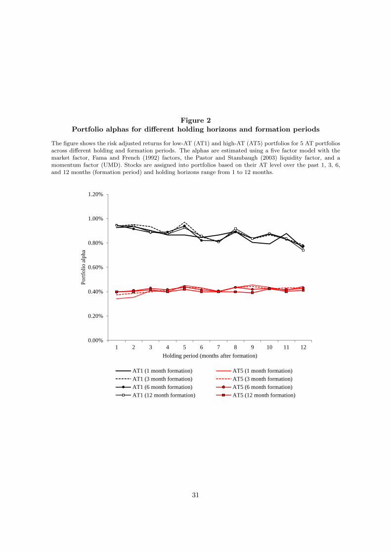
Figure 2Portfolio alphas for different holding horizons and formation periods

The figure shows the risk adjusted returns for low-AT (AT1) and high-AT (AT5) portfolios for 5 AT portfoliosacross different holding and formation periods. The alphas are estimated using a five factor model with themarket factor, Fama and French (1992) factors, the Pastor and Stambaugh (2003) liquidity factor, and amomentum factor (UMD). Stocks are assigned into portfolios based on their AT level over the past 1, 3, 6,and 12 months (formation period) and holding horizons range from 1 to 12 months.

0.00%

0.20%

0.40%

0.60%

0.80%

1.00%

1.20%

1 2 3 4 5 6 7 8 9 10 11 12

Po

rtfo

lio

alp

ha

Holding period (months after formation)

AT1 (1 month formation) AT5 (1 month formation)

AT1 (3 month formation) AT5 (3 month formation)

AT1 (6 month formation) AT5 (6 month formation)

AT1 (12 month formation) AT5 (12 month formation)

31

Appendix

31

Table A.1Variable description

N(quotes)i,t Total number of quote updates in stock i over period t. (Source: TAQ)

N(trades)i,t Total number of trade executions in stock i over period t. (Source: TAQ)

ATi,t =N(quotes)i,tN(trades)i,t

Proxy for algorithmic trading activity for stock i over period t. (Source: TAQ)

N(quotes)HFTi,t Total number of quote updates by 120 HFT firms in stock i over period t on

NASDAQ. (Source: NASDAQ OMX)

N(trades)HFTi,t Total number of trades by 120 HFT firms in stock i over period t on NASDAQ.

(Source: NASDAQ OMX)

ATHFTi,t =

N(quotes)HFTi,t

N(trades)HFTi,t

Measure of algorithmic trading activity for stock i over period t. (Source: NAS-DAQ OMX)

Rf,t Risk free rate, one month Treasury bill rate. (Source: WRDS/Kenneth FrenchWebpage)

Rm,t Value weighted return on the market portfolio (Source: WRDS/Kenneth FrenchWebpage)

Ri,t, Rp,t return on stock i or portfolio p (Source: WRDS/CRSP)

rm,t = Rm,t −Rf,t Excess return on the market. (Source: WRDS/Kenneth French Webpage)

ri,t = Ri,t −Rf,t Excess return on stock i. (Source: WRDS/TAQ)

rp,t = Rp,t −Rf,t Excess return on portfolio p. (Source: WRDS/TAQ)

eri,t Risk adjusted return on stock (or portfolio) i. (Source: WRDS/TAQ)

rhml,t Value factor constructed by Kenneth French. (Source: WRDS/Kenneth FrenchWebpage)

rsmb,t Size factor constructed by Kenneth French. (Source: WRDS/Kenneth FrenchWebpage)

rumd,t Momentum factor (up-minus-down) constructed by Kenneth French. (Source:WRDS/Kenneth French Webpage)

rliq,t Liquidity factor constructed by Pastor and Stambaugh (2003). (Source: WRDS)

QSPREADi,t Quoted spread. Difference between best ask quote and best bid quote (measuredin USD). (Source: TAQ)

SPREADi,t Relative spread. The quoted spread divided by the bid ask midpoint price(measured in %). (Source: TAQ)

PRCi,t Price in USD (Source: WRDS/TAQ)

USDV OLi,t Trading volume in USD (measured in mill. USD) (Source: WRDS/TAQ)

V OLUMEi,t Share volume (measured in mill.) (Source: WRDS/TAQ)

ILRi,t Amihud (2002) illiquidity ratio for stock i over period t calculated as ILRi,t =[∑

(USDvoli,t)/|ri,t|] · 106 (Source: WRDS/TAQ)

V OLAi,t Return volatility for stock i calculated as absolute return over period t. (Source:WRDS/TAQ)

IDIOV OLi,t Idiosyncratic volatility for stock i measured as the standard deviation of theresidual from a three-factor Fama/French model on daily data as in Ang et al.(2009). (Source: WRDS/TAQ)

MCAPi,t Market Capitalization of a stock, calculated as the number of outstanding sharesmultiplied by price. (measured in mill. USD)

BMi,t Book-to-Market value for stock i calculated as the log of the book value of equitydivided by the market value of equity measured for the previous fiscal year.

Analyst following Log of one plus the number of analysts following the firm. (Source: IBES)

Analyst dispersion Log of one plus the dispersion of analyst forecasts divided by the price at yearend. (Source: IBES)

Institutional ownership Holdings of institutions at the end of the year constructed from 13F files.(Source: WRDS) 32

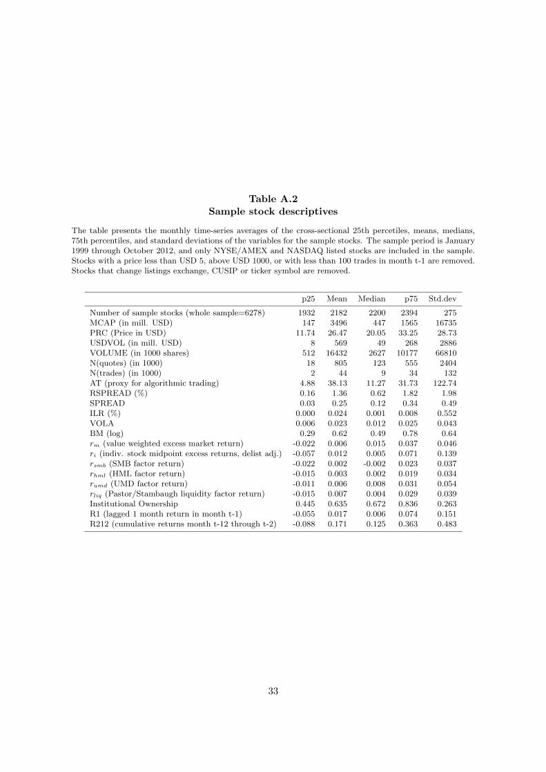
Table A.2Sample stock descriptives

The table presents the monthly time-series averages of the cross-sectional 25th percetiles, means, medians,75th percentiles, and standard deviations of the variables for the sample stocks. The sample period is January1999 through October 2012, and only NYSE/AMEX and NASDAQ listed stocks are included in the sample.Stocks with a price less than USD 5, above USD 1000, or with less than 100 trades in month t-1 are removed.Stocks that change listings exchange, CUSIP or ticker symbol are removed.

p25 Mean Median p75 Std.dev

Number of sample stocks (whole sample=6278) 1932 2182 2200 2394 275MCAP (in mill. USD) 147 3496 447 1565 16735PRC (Price in USD) 11.74 26.47 20.05 33.25 28.73USDVOL (in mill. USD) 8 569 49 268 2886VOLUME (in 1000 shares) 512 16432 2627 10177 66810N(quotes) (in 1000) 18 805 123 555 2404N(trades) (in 1000) 2 44 9 34 132AT (proxy for algorithmic trading) 4.88 38.13 11.27 31.73 122.74RSPREAD (%) 0.16 1.36 0.62 1.82 1.98SPREAD 0.03 0.25 0.12 0.34 0.49ILR (%) 0.000 0.024 0.001 0.008 0.552VOLA 0.006 0.023 0.012 0.025 0.043BM (log) 0.29 0.62 0.49 0.78 0.64rm (value weighted excess market return) -0.022 0.006 0.015 0.037 0.046ri (indiv. stock midpoint excess returns, delist adj.) -0.057 0.012 0.005 0.071 0.139rsmb (SMB factor return) -0.022 0.002 -0.002 0.023 0.037rhml (HML factor return) -0.015 0.003 0.002 0.019 0.034rumd (UMD factor return) -0.011 0.006 0.008 0.031 0.054rliq (Pastor/Stambaugh liquidity factor return) -0.015 0.007 0.004 0.029 0.039Institutional Ownership 0.445 0.635 0.672 0.836 0.263R1 (lagged 1 month return in month t-1) -0.055 0.017 0.006 0.074 0.151R212 (cumulative returns month t-12 through t-2) -0.088 0.171 0.125 0.363 0.483

33

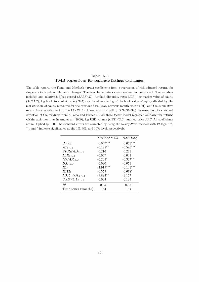
Table A.3FMB regressions for separate listings exchanges

The table reports the Fama and MacBeth (1973) coefficients from a regression of risk adjusted returns for

single stocks listed on different exchanges. The firm characteristics are measured in month t−1. The variables

included are: relative bid/ask spread (SPREAD), Amihud illiquidity ratio (ILR), log market value of equity

(MCAP ), log book to market ratio (BM) calculated as the log of the book value of equity divided by the

market value of equity measured for the previous fiscal year, previous month return (R1), and the cumulative

return from month t − 2 to t − 12 (R212), idiosyncratic volatility (IDIOV OL) measured as the standard

deviation of the residuals from a Fama and French (1992) three factor model regressed on daily raw returns

within each month as in Ang et al. (2009), log USD volume (USDV OL), and log price PRC. All coefficients

are multiplied by 100. The standard errors are corrected by using the Newey-West method with 12 lags. ∗∗∗,∗∗, and ∗ indicate significance at the 1%, 5%, and 10% level, respectively.

NYSE/AMEX NASDAQ

Const. 0.047∗∗∗ 0.063∗∗∗

ATi,t−1 -0.185∗∗ -0.596∗∗∗

SPREADi,t−1 0.216 0.233ILRi,t−1 -0.067 0.041MCAPi,t−1 -0.205∗ -0.337∗∗

BMi,t−1 0.020 -0.053R1i -4.915∗∗∗ -6.143∗∗∗

R212i -0.559 -0.618∗

IDIOV OLi,t−1 -9.884∗∗ -3.167USDV OLi,t−1 0.004 0.124

R2 0.05 0.05Time series (months) 164 164

34

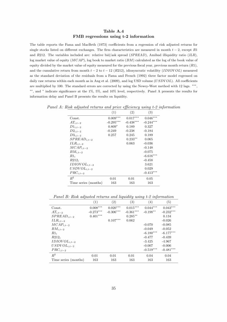
Table A.4FMB regressions using t-2 information

The table reports the Fama and MacBeth (1973) coefficients from a regression of risk adjusted returns for

single stocks listed on different exchanges. The firm characteristics are measured in month t − 2, except R1

and R212. The variables included are: relative bid/ask spread (SPREAD), Amihud illiquidity ratio (ILR),

log market value of equity (MCAP ), log book to market ratio (BM) calculated as the log of the book value of

equity divided by the market value of equity measured for the previous fiscal year, previous month return (R1),

and the cumulative return from month t− 2 to t− 12 (R212), idiosyncratic volatility (IDIOV OL) measured

as the standard deviation of the residuals from a Fama and French (1992) three factor model regressed on

daily raw returns within each month as in Ang et al. (2009), and log USD volume (USDV OL). All coefficients

are multiplied by 100. The standard errors are corrected by using the Newey-West method with 12 lags. ∗∗∗,∗∗, and ∗ indicate significance at the 1%, 5%, and 10% level, respectively. Panel A presents the results for

information delay and Panel B presents the results on liquidity.

Panel A: Risk adjusted returns and price efficiency using t-2 information(1) (2) (3)

Const. 0.009∗∗∗ 0.017∗∗∗ 0.046∗∗∗

ATi,t−2 -0.295∗∗∗ -0.438∗∗∗ -0.244∗∗∗

D1i,t−2 0.809∗ 0.189 0.327D2i,t−2 -0.249 -0.238 -0.184D3i,t−2 0.257 0.245 0.189SPREADi,t−2 0.233∗∗ 0.065ILRi,t−2 0.063 -0.036MCAPi,t−2 -0.148BMi,t−2 -0.075R1i -6.616∗∗∗

R212i -0.458IDIOV OLi,t−2 3.621USDV OLi,t−2 0.029PRCi,t−2 -0.413∗∗∗

R2 0.01 0.01 0.05Time series (months) 163 163 163

Panel B: Risk adjusted returns and liquidity using t-2 information(1) (2) (3) (4) (5)

Const. 0.008∗∗∗ 0.020∗∗∗ 0.015∗∗∗ 0.044∗∗∗ 0.043∗∗∗

ATi,t−2 -0.273∗∗∗ -0.306∗∗∗ -0.361∗∗∗ -0.198∗∗ -0.232∗∗∗

SPREADi,t−2 0.401∗∗∗ 0.285∗∗ 0.134ILRi,t−2 0.107∗∗∗ 0.062 -0.026MCAPi,t−2 -0.070 -0.085BMi,t−2 -0.049 -0.052R1i -6.180∗∗∗ -6.177∗∗∗

R212i -0.477 -0.439IDIOV OLi,t−2 -3.425 -4.967USDV OLi,t−2 -0.007 -0.006PRCi,t−2 -0.519∗∗∗ -0.481∗∗∗

R2 0.01 0.01 0.01 0.04 0.04Time series (months) 163 163 163 163 163

35

References

Amihud, Y. (2002). “Illiquidity and stock returns:Cross-section and time-series effects.” Journal ofFinancial Markets, 5, 31 – 56.

Amihud, Y. and H. Mendelson (1986). “Asset pric-ing and the bid-ask spread.” Journal of FinancialEconomics, 17, 223–249.

Ang, A., R. J. Hodrick, Y. Xing, and X. Zhang (2009).“High idiosyncratic volatility and low returns: In-ternational and further U.S. evidence.” Journal ofFinancial Economics, 91, 1–23.

Asparouhova, E., H. Bessembinder, and I. Kalcheva(2010). “Liquidity biases in asset pricing tests.”Journal of Financial Economics, 96, 215–237.

Asparouhova, E., H. Bessembinder, and I. Kalcheva(2013). “Noisy prices and inference regarding re-turns.” Journal of Finance, 68.

Biais, B., T. Foucault, and S. Moinas (2011). “Equi-librium algorithmic trading.” Working paper, IDEIToulouse School of Economics.

Biais, B., J. Hombert, and P.-O. Weill (2010). “Trad-ing and liquidity with limited cognition.” WorkingPaper 16628, NBER.

Biais, B. and P. Woolley (2011). “High frequency trad-ing.” Working paper, IDEI Toulouse School of Eco-nomics.

Boehmer, E., K. Y. L. Fong, and J. J. Wu (2012).“International evidence on algorithmic trading.”Working papers series, EDHEC Business School.

Brennan, M. and A. Subrahmanyam (1996). “Marketmicrostructure and asset pricing: On the compen-sation for illiquidity in stock returns.” Journal ofFinancial Economics, 41, 441–464.

Brennan, M. J., T. Chordia, and A. Subrahmanyam(1998). “Alternative factor specifications, securitycharacteristics and the cross-section of expectedstock returns.” Journal of Financial Economics,49, 345–373.

Brennan, M. J., T. Chordia, A. Subrahmanyam, andQ. Tong (2012). “Sell-order liquidity and the cross-section of expected stock returns.” Journal of Fi-nancial Economics, 105, 523 – 541.

Brogaard, J., T. Hendershott, and R. Riordan (2013).“High frequency trading and price discovery.” Re-view of Financial Studies, forthcoming.

Chaboud, A., B. Chiquoine, E. Hjalmarsson, andC. Vega (2009). “Rise of the machines: Algorithmictrading in the foreign exchange market.” Workingpaper, FRB International Finance.

Chordia, T., R. Roll, and A. Subrahmanyam (2000).“Commonality in liquidity.” Journal of FinancialEconomics, 56, 3 – 28.

Chordia, T., R. Roll, and A. Subrahmanyam (2002a).“Order imbalance, liquidity, and market returns.”Journal of Financial Economics, 65, 111–130.

Chordia, T., A. Subrahmanyam, and V. Anshuman(2002b). “Trading activity and expected stock re-turns.” Journal of Financial Economics, 59, 3–32.

Chordia, T., A. Subrahmanyam, and Q. Tong (2011).“Trends in the cross-section of expected stock re-turns.” Working paper.

Domowitz, I. and H. Yegerman (2005). “The cost ofalgorithmic trading: A first look at comparativeperformance.” In B. R. Bruce (Ed.), “AlgorithmicTrading: Precision, Control, Execution,” Institu-tional Investor.

Duarte, J. and L. Young (2009). “Why is PIN priced?”Journal of Financial Economics, 91, 119–138.

Easley, D., S. Hvidkjaer, and M. O’Hara (2002). “Isinformation risk a determinant of asset returns?”Journal of Finance, 57, 2185–2221.

Easley, D. and M. O’Hara (2004). “Information andthe cost of capital.” Journal of Finance, 59, 1553–1583.

Engle, R., R. Ferstenberg, and J. Russell (2012).“Measuring and modeling execution cost and risk.”Journal of Portfolio Management, 38, 14–28.

Fama, E. and J. MacBeth (1973). “Risk, return, andequilibrium: Empirical tests.” Journal of PoliticalEconomy, 81, 607–636.

Fama, E. F. and K. R. French (1992). “The cross-section of expected stock returns.” Journal of Fi-nance, 47, 427–465.

Foucault, T., J. Hombert, and I. Rosu (2012). “Newstrading and speed.” Working paper, HEC Paris.

Goyenko, R. Y., C. W. Holden, and C. A. Trzcinka(2009). “Do liquidity measures measure liquidity?”Journal of Financial Economics, 92, 153 – 181.

Hagstromer, B. and L. Norden (2013). “The diversityof high-frequency traders.” Journal of FinancialMarkets, forthcoming.

Hasbrouck, J. (2009). “Trading costs and returns forU.S. equities: Estimating effective costs from dailydata.” Journal of Finance, 64, 1445–1477.

Hasbrouck, J. and G. Saar (2013). “Low-latency trad-ing.” Journal of Financial Markets, 16, 645–678.

36

Hendershott, T., C. M. Jones, and A. J. Menkveld(2011). “Does algorithmic trading improve liquid-ity.” Journal of Finance, 66, 1–33.

Hendershott, T. and R. Riordan (2012). “Algorithmictrading and information.” Journal of Financial andQuantitative Analysis.

Hou, K. and T. Moskowitz (2005). “Market frictions,price delay and the cross-section of expected re-turns.” Review of Financial Studies, 18, 981–1020.

Jones, C. (2002). “A century of stock market liquid-ity and trading costs.” Working paper, ColumbiaBusiness School.

Jones, C. M. (2013). “What do we know about high-frequency trading?” Working paper, ColumbiaBusiness School.

Jovanovic, B. and A. Menkveld (2010). “Middlemenin limit-order markets.” Working paper, New YorkUniversity.

Khandan, A. E. and A. Lo (2011). “What happenedto the quants in august 2007? Evidence from fac-tors and transactions data.” Journal of FinancialMarkets, 14, 1–46.

Kirilenko, A., A. Kyle, M. Samadi, and T. Tuzun(2012). “The flash crash: The impact of high fre-quency trading on an electronic market.” Workingpaper, University of Maryland.

Menkveld, A. (2013). “High-frequency trading and thenew market makers.” Journal of Financial Mar-kets, forthcoming.

O’Hara, M. (2003). “Liquidity and price discovery.”Journal of Finance, 58, 1335–1354.

Pastor, L. and R. F. Stambaugh (2003). “Liquidityrisk and expected stock returns.” Journal of Polit-ical Economy, 111, 642–685.

Shumway, T. (1997). “The delisting bias in CRSPdata.” Journal of Finance, 52, 327–340.

37