Trading the Stock Market using Google

Search Volumes A Long Short-Term Memory Approach

by

Joseph St. Pierre

Mateusz Klimkiewicz

Adonay Resom

Nikolaos Kalampalikis

Abstract

In this paper, we present a methodology for utilizing Google Search Indices obtained from the

Google Trends website as a means for measuring potential investor interest in stocks listed on the Dow

Jones Index (Dow 30). We accomplish this task by utilizing a Long Short-Term Memory network that

correlates changes in the search volume for a given asset with changes in the actual trade volume for said

asset. Additionally, by using these predictions, we formulate a concise trading strategy in the hopes of

being able to outperform the market and analyze the results of this new strategy by backtesting across

weekly closing price data for the last six months of 2016. With these tests, it was discovered that about

43% of the time, the machine learning based trading strategy outperformed the baseline sample indicating

that there is indeed a correlation between price movements for certain assets on the Dow 30 and the

number of Google searches for said assets. Furthermore, while the scope of our study was limited to the

Dow 30 in order to mitigate selection bias, we nonetheless hypothesize that numerous other assets that

similarly possess a predictable correlation to Google Search Volumes are likely to exist thereby making

the trading algorithm described in this paper applicable beyond the narrow scope of this study.

1. Introduction

The market cannot be outperformed. This is perhaps the most commonly accepted theory

stemming from the Efficient Market Hypothesis (EMH). Namely, it postulates that predictions about the

market cannot be made and that any strategies that appear to be outperforming the market are in fact

attributed more to chance rather than the skill of the trader. In the 1960s, Eugene Fama authored a

dissertation that later evolved into the EMH: a theory that is commonly accepted as the fundamental law

of the stock exchange (Nath, 2015). Fama wrote that the market is only efficient if the price of an asset is

representative of all available information (Fama, 1970). From this perspective, the EMH was created as a

theory with three iterations ranging from weak, semi-strong, to strong. Weak EMH suggests that all

currently available public information is already accounted for in the stock price, and thus, predicting the

future price of an asset is futile. Semi-strong EMH suggests that both technical and fundamental analysis

cannot help in achieving returns above the market return. Finally, the strong theory suggests that any and

all data available, including private data, is already represented in the stock price (Nath, 2015). However,

this theory does have its shortcomings. For example, it is possible that investors may value information

differently, and even, when given the exact same data, may come to completely different conclusions

about a stock’s value depending on where their biases lie. Furthermore, if the theory were entirely true,

investing in stocks would not necessarily be profitable, as every investor would act similarly in terms of

their trading activity and the timing for such trades (Van Bergen, 2011).

While EMH may have been applicable throughout a large portion of the 20th century, the

commencement of the information era gave way to all types of information becoming accessible to the

general public through the usage of computers and the Internet. Since the 1980s, when the public’s use of

technology began (Rouse, 2014), EMH theory, which was developed in the late 60s, may not hold true

any longer due to arbitrage or other such opportunities. Moreover, since the Internet is accessible to

everyone, everyone can instantly access news and data as they are released along with the extent to which

information is searched for by users all around the world. One such provider of online search metrics is

Google who, through the development and deployment of their Google Trends website, has provided the

average person with the ability to monitor the Internet habits of their fellow countrymen and those of

foreign nations. Despite the fact that this Orwellian reality might be considered unsettling to some, it

nonetheless provides an avenue for measuring the aggregate interests of Internet users leading to the

capacity for investors to gauge the relevancy of certain assets with respect to society at large.

Can this newfound ability to access information be of any use to investors? According to the

EMH, these search metrics should already be accounted for in the market; thereby, nullifying any

potential benefits of their utilization for the investor. Whether this is true at its core, it is practically

applicable, as such a large amount of data would be close to impossible for a single person to process

meaningfully due to the widespread existence of random statistical noise. This is a human inadequacy

however, one which might be capable of being circumvented through the usage of Artificial Intelligence

(AI). If an AI could be taught to seek out and correlate patterns between the Google Search Volume

(GSV) for a given asset and the historical data for said asset, a trading strategy could theoretically be

formulated using the predictions of said AI as an indicator for determining which actions investors should

take with respect to the market.

To test this conjecture, a group of companies was chosen for the experiment in an unbiased

manner. While there are potentially several ways of accomplishing this task, the Dow 30 was chosen due

to its sampling size, investor interest, and distribution of industry representation. Additionally, in order to

measure the efficacy of any new trading strategy, a baseline is required for comparing the results of said

strategy to those of an already commonly used and existing strategy. As such, we decided that the strategy

of Buy and Hold would be an adequate comparison as it is a simple yet effective strategy that any patient

individual can understand and utilize on typically steadfast stocks, as in the case of the Dow 30 (Carlson,

2015).

Once our dataset was decided upon, we set out to create an automated trading algorithm utilizing

a Long Short-Term Memory (LSTM) network's predictions as an indicator for future market movements.

This "auto-trader," which we present in our paper, operates on a weekly basis, choosing to either buy, sell,

or hold a given asset based on the predictions made by its LSTM network in conjunction with a

continuously updated moving average and standard deviation. The strategy employed by this "auto-

trader" could be described as contrarian, as it actively seeks to avoid holding on to an asset during

projected periods of market instability as indicated by its LSTM network.

The strategy initially used daily sets of GSVs and closing prices to train its LSTM network.

However, due to discrepancies found between daily datasets, initial results were not promising. Therefore,

daily sets were replaced by weekly sets, and the strategy was tested again. This time, the results were far

better, as the auto-trader was able to outperform the Buy and Hold strategy for 12 out of the chosen 28

Dow 30 companies. The overall performance of the strategy could perhaps be improved further with the

usage of more detailed data sets. For example, daily GSVs that do not contain discrepancies between sets

could increase the strategy’s performance. Thus, with such improvements towards the strategy, it could be

possible to create trading systems that can disprove the EMH.

2. Data

In order to train the LSTM network and backtest the trading strategy utilized by the auto-trader,

weekly GSVs, trade volumes, and closing prices were collected for each stock over a span of five years.

However, the above data requirements were not met for all 30 companies. Specifically, Travelers

Companies, Inc., and DowDuPont, Inc., were excluded due to a lack of Google Trends data, leaving a

total of 28 companies to be tested. In the case of DowDuPont, Inc., the reason as to the lack of data was

quite obvious: Just under two years ago, the two companies (Dow and Dupont) merged into one, and thus,

there was not even two years of data on Google Trends to be trained and backtested against as the

company simply has not existed for five years yet. Despite this shortcoming, for the remaining 28 stocks,

the neural network was trained using pairs of weekly GSV and trade volume for each and every asset.

2.1 Google Search Volume

Google Trends data is normalized with respect to the timeframe selected, and the value of each

index at every timestep ranges between 0 (lowest) and 100 (highest). The value of a Google Search Index

represents the relative interest of a particular Google search with respect to the highest number of

searches in the selected time period. Any value contained in a Google Trends dataset represents the

percentage of the highest number of searches (i.e. a Google Search Index of 50 indicates that the total

number of searches at that particular timestep is approximately 50% of the maximum number of searches

recorded at any time within the selected timeframe)1. In other words, Google Search Indices, even when

referring to the same timestep, will differ depending on the overall timeframe selected (Rogers, 2016).

The goal of our data collection was to gather the maximum amount of data possible for a

continuous time period, so that later we could have a bigger data set for training and testing. However,

since Google Trends arbitrarily enforces an upper limit on timeframes for weekly data, only five years’

worth of GSVs were able to be utilized in our study. This time period starts on January 1, 2012, and

extends to January 1, 2017, as data earlier than that was deemed to be insufficient due to changes made by

Google concerning the manner in which Google Search Indices were calculated, and a partial year was

undesired. Once an appropriate timeframe for our study was decided upon, the task of choosing exactly

which search terms to analyze was upon us. The first idea was to simply use the company name; however,

this proved to be problematic as there was no straightforward way to differentiate between investors

searching for assets to purchase and ordinary consumers seeking to conduct business with the company

just from the Google Search Index alone. Therefore, it was decided that the best way to have a reliable

and meaningful search term was to use the company’s stock symbol followed by the string: “Stock Price”

(i.e. instead of searching for “Apple,” we searched for “AAPL Stock Price”). This ensured that the values

for each Google Search Index were likely only representing potential investors interested in purchasing

one of the 28 stocks being considered.

2.2 Sample Size

1. 1 How Trends data is adjusted - Trends Help. (n.d.). Retrieved October 29, 2017, from

https://support.google.com/trends/answer/4365533?hl=en

The resulting sample size, used for training and testing the network, consisted of 260 pairs of

weekly Google Search Indices and their corresponding trade volumes for each of the 28 stocks. Since the

purpose of the LSTM network was to correlate a change in GSV at time t with a subsequent change in

trade volume at time t+1, the last Google Search index was removed from the Google Trends dataset for

each stock (since there is no corresponding trade volume at time t+1 to predict), and the first trade

volume from the trade volumes dataset for each stock was also removed (since there is no preceding

Google Search Index to be used for predicting it). This left each of the remaining datasets with exactly

259 entries.

Once the datasets had been properly prepared for all 28 stocks, the task of partitioning up our data

into subsets for training and testing presented itself. Due to the rather small sample size in question, this

problem posed an interesting dilemma. On the one hand, in order to properly backtest our trading

algorithm, we needed a significant portion of the data to be used for testing purposes so as to reasonably

assess the fitness and relevancy of our findings. However, in direct contention with this requirement was

the need for the LSTM network to have enough data during training to be able to make meaningful

predictions off of the test data to which it would later be presented. After some deliberation and initial

testing, it was decided that 90% (4.5 years) of each dataset would be used for training the LSTM network

to predict future trade volumes, leaving 10% (0.5 years) for backtesting the trading algorithm utilized by

the auto-trader. While it cannot be asserted that this is the optimal partitioning method for resolving the

aforementioned constraints, there is, as of today, no deterministic way of training a neural network to

guarantee a particular predictability of success. Therefore, for the purposes of our study, the

aforementioned 90:10 training to testing set cardinality ratio was deemed sufficient (Pasini, 2015).

2.3 Training to testing set cardinality ratio

In a more methodological analysis of the trade volume prediction, a larger set would be required

for the neural network to be trained and tested. As there is no concern for a neural network to be over

tested, the main goal is to prevent a neural network from overfitting (overtraining) or underfitting its

weight matrices to its training data, especially in a nonlinear system. If a neural network is undertrained, it

will fail to make sense of its testing data as it will not have had enough exposure to the outputs of the

unknown function with which it is attempting to approximate. Conversely, in the event that a neural

network is overtrained, it will similarly fail to accurately predict its testing data; however, this failure is

not a result of a lack of exposure, but rather is attributed to the fact that the network is too privy to just a

subset of the hidden function which it is trying to approximate and, as a result, has lost sight of the bigger

picture and its ability to extrapolate (Pasini, 2015).

Clearly, in the case of our study, undertraining the neural network posed the larger concern. Due

to the shortage of reliable weekly GSVs and the technical difficulties which prevented daily data

extraction, it was decided that the majority of the data tuples would be used for the training of the neural

network, while still maintaining a reasonable amount of testing data: secure enough to lead us to the

following speculations.

3. Methodology

3.1 Overview

When it comes to prediction problems over timed intervals, the classical variant of perceptron

based neural networks prove themselves to be completely inadequate. While such architectures provide

excellent utility with respect to discrete classification problems such as image and handwriting

recognition (Egmont-Petersen, 2002), the problem of correlating time-intervaled data and basing future

predictions off of said data requires a fundamentally different approach to machine learning. This

alternative approach is known as LSTM.

3.2 Long Short-Term Memory

3.2.1 Why LSTM?

LSTM is a type of Recurrent Neural Network (RNN) first introduced by Sepp Hochreiter and

Jürgen Schmidhuber in 1997 as a means to solve the vanishing gradient problem (Bengio, 1994) that

plagued other RNN architectures of the time. Prior to its introduction, problems which required neural

networks to "remember" relevant prior stimuli, such as in the case of speech recognition, were proving

themselves to be computationally infeasible to solve for even the most sophisticated of training

algorithms (Hochreiter, 1997). Since their publication however, LSTM networks have been used to solve

a wide variety of hard prediction problems such as phoneme classification (Graves, 2005), context-free

and context-sensitive language processing (Gers, 2001), and perhaps most importantly as far as this paper

is concerned, time series prediction as in the case of stock price forecasting (Bao, 2017). These promising

developments have brought LSTM networks to the forefront of modern AI research in the hopes of

finding the limits of their potential.

3.2.2 Diagram and Component Specification

LSTM networks are comprised of a sequential ordering of interconnected identical blocks. Each

of these blocks contain a cell, a forget gate, an input gate, and an output gate, each of which possesses a

weight matrix that is updated during training. When data is presented to the network, it is fed into the first

block, processed, and subsequently passed onto the next block in the chain for processing. This process is

repeated until the last block of the LSTM returns a value that is dependent on all of the blocks' individual

processing of the data. In order to understand the significance and utility of constructing a neural network

in this manner, it is necessary to examine the exact method by which an LSTM block receives input,

processes the input based off of past experience, and updates its own composition based off of what was

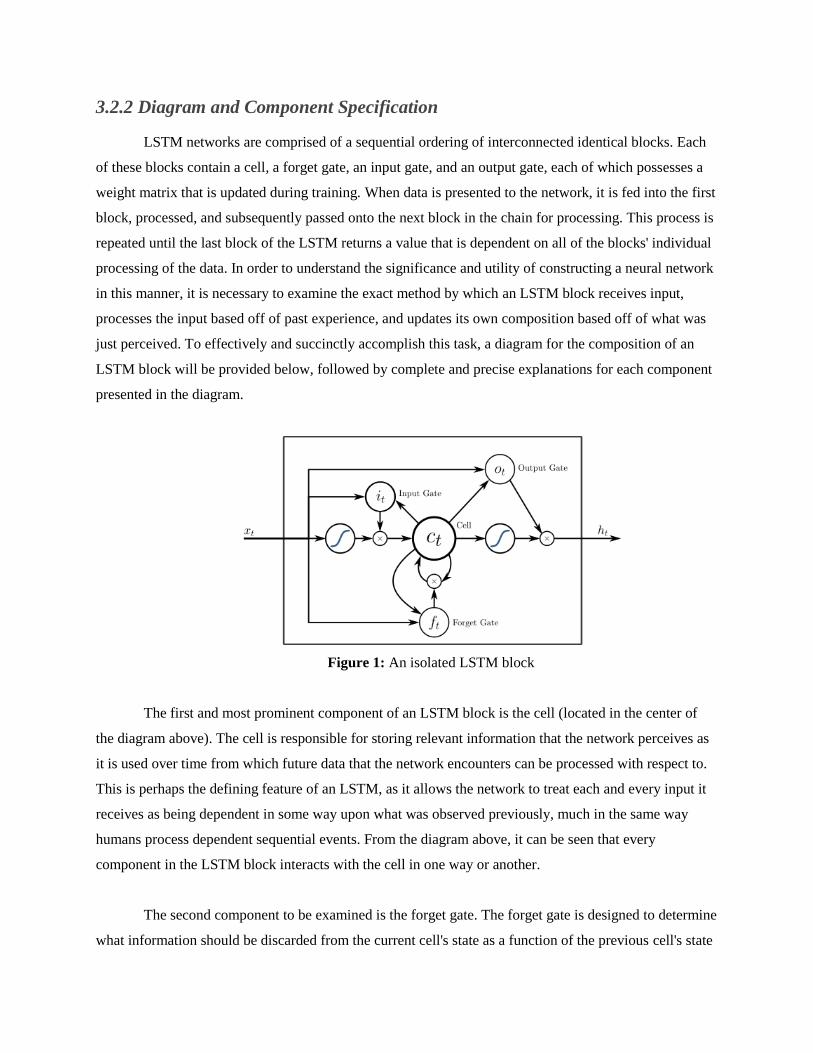
just perceived. To effectively and succinctly accomplish this task, a diagram for the composition of an

LSTM block will be provided below, followed by complete and precise explanations for each component

presented in the diagram.

Figure 1: An isolated LSTM block

The first and most prominent component of an LSTM block is the cell (located in the center of

the diagram above). The cell is responsible for storing relevant information that the network perceives as

it is used over time from which future data that the network encounters can be processed with respect to.

This is perhaps the defining feature of an LSTM, as it allows the network to treat each and every input it

receives as being dependent in some way upon what was observed previously, much in the same way

humans process dependent sequential events. From the diagram above, it can be seen that every

component in the LSTM block interacts with the cell in one way or another.

The second component to be examined is the forget gate. The forget gate is designed to determine

what information should be discarded from the current cell's state as a function of the previous cell's state

and the current input provided to the LSTM block. This component can be considered as the process by

which irrelevant or outdated data are pruned from being utilized for future computations by the network.

A good example of the potential use for this component is in the domain of natural language processing;

namely, if the network is processing a paragraph and detects a new subject, it should forget the gender of

the previous subject.

The third component is the input gate. The input gate handles the manner in which the current

cell's state is updated as a function of the previous cell's state and current input to the LSTM block. The

purpose of this component is to provide a well-defined manner by which new information is introduced to

the cell such that prior critical information is not lost, and there is not an inordinate amount of junk data

added to the cell's state.

The last major component is the output gate which simply controls what portion of the cell's state

is to be used in conjunction with the provided input data for the production of the LSTM block's output.

Since it is almost never desirable to use the entirety of the cell state when determining the subsequent

output for the block, there needs to be a well-defined mechanism that can prune unnecessary information

from the current cell's state from being considered for output as a function of the previous cell's state and

current input to the LSTM block.

3.2.3 Mathematical Formulation

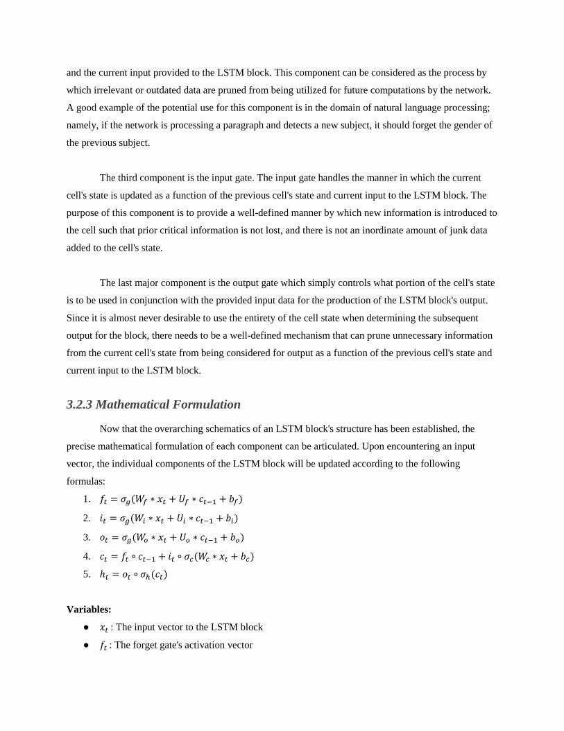
Now that the overarching schematics of an LSTM block's structure has been established, the

precise mathematical formulation of each component can be articulated. Upon encountering an input

vector, the individual components of the LSTM block will be updated according to the following

formulas:

1. 𝑓𝑡 = 𝜎𝑔(𝑊𝑓 ∗ 𝑥𝑡 + 𝑈𝑓 ∗ 𝑐𝑡−1 + 𝑏𝑓)

2. 𝑖𝑡 = 𝜎𝑔(𝑊𝑖 ∗ 𝑥𝑡 + 𝑈𝑖 ∗ 𝑐𝑡−1 + 𝑏𝑖)

3. 𝑜𝑡 = 𝜎𝑔(𝑊𝑜 ∗ 𝑥𝑡 + 𝑈𝑜 ∗ 𝑐𝑡−1 + 𝑏𝑜)

4. 𝑐𝑡 = 𝑓𝑡 ∘ 𝑐𝑡−1 + 𝑖𝑡 ∘ 𝜎𝑐(𝑊𝑐 ∗ 𝑥𝑡 + 𝑏𝑐)

5. ℎ𝑡 = 𝑜𝑡 ∘ 𝜎ℎ(𝑐𝑡)

Variables:

● 𝑥𝑡 : The input vector to the LSTM block

● 𝑓𝑡 : The forget gate's activation vector

● 𝑖𝑡 : The input gate's activation vector

● 𝑜𝑡: The output gate's activation vector

● ℎ𝑡: The output vector of the LSTM block

● 𝑐𝑡: The cell state vector

● W, U, and b: The weight matrices and bias vector parameters to be learned during training

3.3 Specification and Training

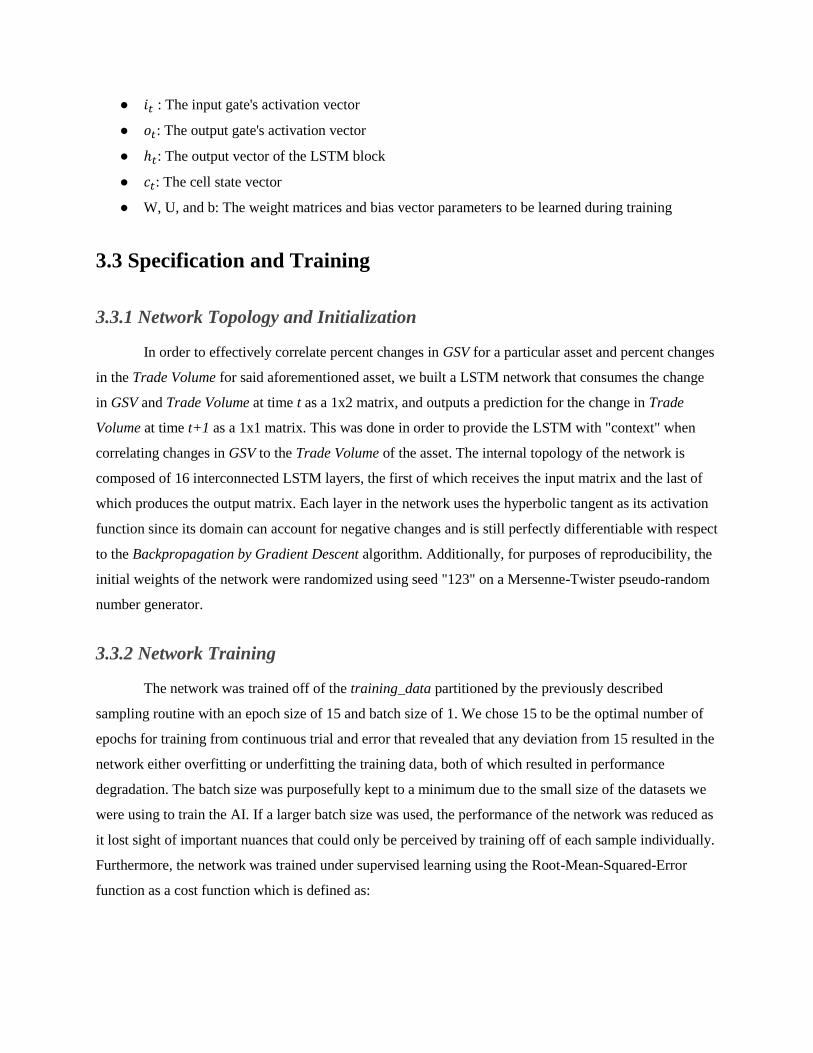
3.3.1 Network Topology and Initialization

In order to effectively correlate percent changes in GSV for a particular asset and percent changes

in the Trade Volume for said aforementioned asset, we built a LSTM network that consumes the change

in GSV and Trade Volume at time t as a 1x2 matrix, and outputs a prediction for the change in Trade

Volume at time t+1 as a 1x1 matrix. This was done in order to provide the LSTM with "context" when

correlating changes in GSV to the Trade Volume of the asset. The internal topology of the network is

composed of 16 interconnected LSTM layers, the first of which receives the input matrix and the last of

which produces the output matrix. Each layer in the network uses the hyperbolic tangent as its activation

function since its domain can account for negative changes and is still perfectly differentiable with respect

to the Backpropagation by Gradient Descent algorithm. Additionally, for purposes of reproducibility, the

initial weights of the network were randomized using seed "123" on a Mersenne-Twister pseudo-random

number generator.

3.3.2 Network Training

The network was trained off of the training_data partitioned by the previously described

sampling routine with an epoch size of 15 and batch size of 1. We chose 15 to be the optimal number of

epochs for training from continuous trial and error that revealed that any deviation from 15 resulted in the

network either overfitting or underfitting the training data, both of which resulted in performance

degradation. The batch size was purposefully kept to a minimum due to the small size of the datasets we

were using to train the AI. If a larger batch size was used, the performance of the network was reduced as

it lost sight of important nuances that could only be perceived by training off of each sample individually.

Furthermore, the network was trained under supervised learning using the Root-Mean-Squared-Error

function as a cost function which is defined as:

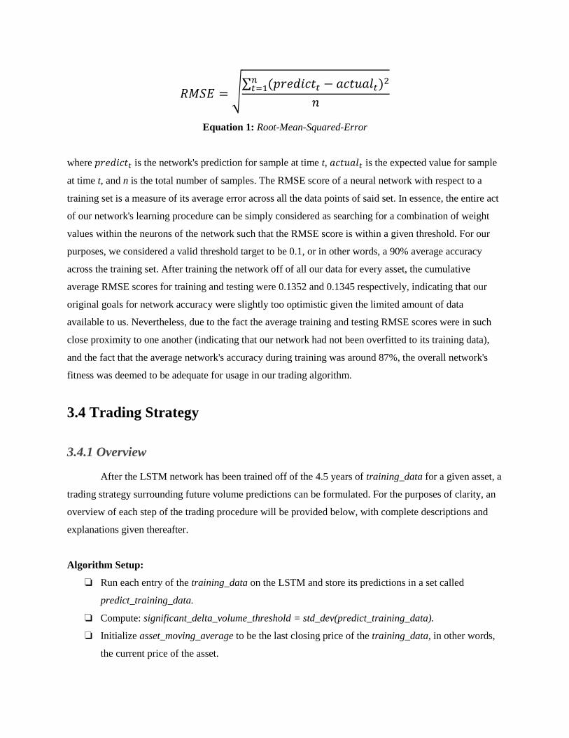
𝑅𝑀𝑆𝐸 = √∑ (𝑝𝑟𝑒𝑑𝑖𝑐𝑡𝑡 − 𝑎𝑐𝑡𝑢𝑎𝑙𝑡)2𝑛

𝑡=1

𝑛

Equation 1: Root-Mean-Squared-Error

where 𝑝𝑟𝑒𝑑𝑖𝑐𝑡𝑡 is the network's prediction for sample at time t, 𝑎𝑐𝑡𝑢𝑎𝑙𝑡 is the expected value for sample

at time t, and n is the total number of samples. The RMSE score of a neural network with respect to a

training set is a measure of its average error across all the data points of said set. In essence, the entire act

of our network's learning procedure can be simply considered as searching for a combination of weight

values within the neurons of the network such that the RMSE score is within a given threshold. For our

purposes, we considered a valid threshold target to be 0.1, or in other words, a 90% average accuracy

across the training set. After training the network off of all our data for every asset, the cumulative

average RMSE scores for training and testing were 0.1352 and 0.1345 respectively, indicating that our

original goals for network accuracy were slightly too optimistic given the limited amount of data

available to us. Nevertheless, due to the fact the average training and testing RMSE scores were in such

close proximity to one another (indicating that our network had not been overfitted to its training data),

and the fact that the average network's accuracy during training was around 87%, the overall network's

fitness was deemed to be adequate for usage in our trading algorithm.

3.4 Trading Strategy

3.4.1 Overview

After the LSTM network has been trained off of the 4.5 years of training_data for a given asset, a

trading strategy surrounding future volume predictions can be formulated. For the purposes of clarity, an

overview of each step of the trading procedure will be provided below, with complete descriptions and

explanations given thereafter.

Algorithm Setup:

❏ Run each entry of the training_data on the LSTM and store its predictions in a set called

predict_training_data.

❏ Compute: significant_delta_volume_threshold = std_dev(predict_training_data).

❏ Initialize asset_moving_average to be the last closing price of the training_data, in other words,

the current price of the asset.

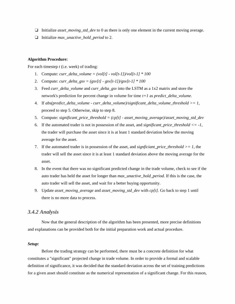
❏ Initialize asset_moving_std_dev to 0 as there is only one element in the current moving average.

❏ Initialize max_unactive_hold_period to 2.

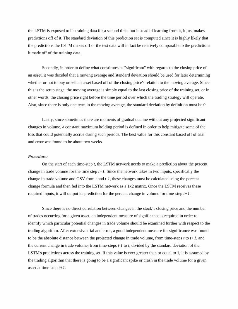
Algorithm Procedure:

For each timestep t (i.e. week) of trading:

1. Compute: curr_delta_volume = (vol[t] - vol[t-1])/vol[t-1] * 100

2. Compute: curr_delta_gsv = (gsv[t] - gsv[t-1])/gsv[t-1] * 100

3. Feed curr_delta_volume and curr_delta_gsv into the LSTM as a 1x2 matrix and store the

network's prediction for percent change in volume for time t+1 as predict_delta_volume.

4. If abs(predict_delta_volume - curr_delta_volume)/significant_delta_volume_threshold >= 1,

proceed to step 5. Otherwise, skip to step 8.

5. Compute: significant_price_threshold = (cp[t] - asset_moving_average)/asset_moving_std_dev

6. If the automated trader is not in possession of the asset, and significant_price_threshold <= -1,

the trader will purchase the asset since it is at least 1 standard deviation below the moving

average for the asset.

7. If the automated trader is in possession of the asset, and signficiant_price_threshold >= 1, the

trader will sell the asset since it is at least 1 standard deviation above the moving average for the

asset.

8. In the event that there was no significant predicted change in the trade volume, check to see if the

auto trader has held the asset for longer than max_unactive_hold_period. If this is the case, the

auto trader will sell the asset, and wait for a better buying opportunity.

9. Update asset_moving_average and asset_moving_std_dev with cp[t]. Go back to step 1 until

there is no more data to process.

3.4.2 Analysis

Now that the general description of the algorithm has been presented, more precise definitions

and explanations can be provided both for the initial preparation work and actual procedure.

Setup:

Before the trading strategy can be performed, there must be a concrete definition for what

constitutes a "significant" projected change in trade volume. In order to provide a formal and scalable

definition of significance, it was decided that the standard deviation across the set of training predictions

for a given asset should constitute as the numerical representation of a significant change. For this reason,

the LSTM is exposed to its training data for a second time, but instead of learning from it, it just makes

predictions off of it. The standard deviation of this prediction set is computed since it is highly likely that

the predictions the LSTM makes off of the test data will in fact be relatively comparable to the predictions

it made off of the training data.

Secondly, in order to define what constitutes as "significant" with regards to the closing price of

an asset, it was decided that a moving average and standard deviation should be used for later determining

whether or not to buy or sell an asset based off of the closing price's relation to the moving average. Since

this is the setup stage, the moving average is simply equal to the last closing price of the training set, or in

other words, the closing price right before the time period over which the trading strategy will operate.

Also, since there is only one term in the moving average, the standard deviation by definition must be 0.

Lastly, since sometimes there are moments of gradual decline without any projected significant

changes in volume, a constant maximum holding period is defined in order to help mitigate some of the

loss that could potentially accrue during such periods. The best value for this constant based off of trial

and error was found to be about two weeks.

Procedure:

On the start of each time-step t, the LSTM network needs to make a prediction about the percent

change in trade volume for the time step t+1. Since the network takes in two inputs, specifically the

change in trade volume and GSV from t and t-1, these changes must be calculated using the percent

change formula and then fed into the LSTM network as a 1x2 matrix. Once the LSTM receives these

required inputs, it will output its prediction for the percent change in volume for time-step t+1.

Since there is no direct correlation between changes in the stock’s closing price and the number

of trades occurring for a given asset, an independent measure of significance is required in order to

identify which particular potential changes in trade volume should be examined further with respect to the

trading algorithm. After extensive trial and error, a good independent measure for significance was found

to be the absolute distance between the projected change in trade volume, from time-steps t to t+1, and

the current change in trade volume, from time-steps t-1 to t, divided by the standard deviation of the

LSTM's predictions across the training set. If this value is ever greater than or equal to 1, it is assumed by

the trading algorithm that there is going to be a significant spike or crash in the trade volume for a given

asset at time-step t+1.

In the event that a significant change in trade volume is predicted, the trading algorithm must

make a decision with respect to buying, selling, or holding the asset. The algorithm makes this decision

based off of the assumption that when an asset is at a relative low or high with respect to the moving

average, there is a chance for a dramatic shift in the price of said asset at time-step t+1. Furthermore, it

operates on the assumption that when the asset is priced at either of these extremes, the probability of this

dramatic price shift being in the direction of the moving average is greater than the probability of the

closing price moving further away from the moving average. In other words, the algorithm is attempting

to avoid instabilities in the market that are a result of high trade volumes.

Despite the usefulness of LSTM's for predicting time-intervaled data, they are not always correct,

and it is impossible to formally prove the correctness of their predictions. As such, it is entirely possible

for the LSTM to not make predictions that are deemed significant for long stretches of time. While this

does not necessarily pose a problem for determining when to purchase and hold an asset, it can lead to

issues with regards to selling an asset. For this reason, if the LSTM does not predict a significant volume

spike for more than the defined max_unactive_hold_period, the trading algorithm will simply sell its

shares and wait for another predicted volume spike to occur.

Lastly, at the end of each time-step, the moving average and standard deviation must be updated

for use during future time-steps.

4. Findings

4.1 Initial Findings

The original goal for this research was to predict the closing prices of stocks through GSV samples.

Therefore, the LSTM network was initially trained with sets of daily GSV and closing price data. The

network was able to detect a visible correlation between the two datasets; however, it had a low success

rate of accurately predicting weekly stock prices for the companies that comprise the Dow 30. As a result,

the relationship was found to be insufficient for implementing the trading strategy we formulated. Before

this conclusion was made, the same trading strategy was used to simulate day to day trading using daily

GSV data from the latter half of 2016. Most returns from that experiment were lower than returns that could

have been produced via the Buy and Hold trading strategy.

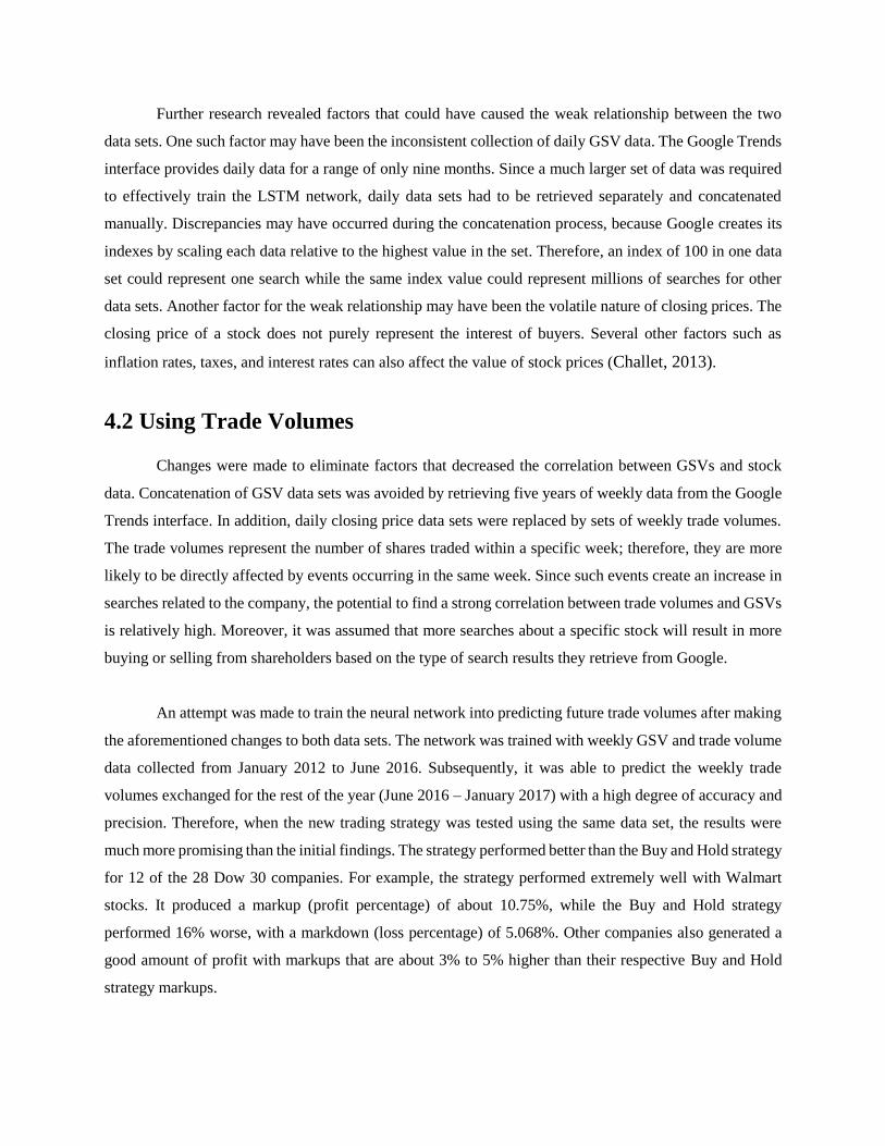
Further research revealed factors that could have caused the weak relationship between the two

data sets. One such factor may have been the inconsistent collection of daily GSV data. The Google Trends

interface provides daily data for a range of only nine months. Since a much larger set of data was required

to effectively train the LSTM network, daily data sets had to be retrieved separately and concatenated

manually. Discrepancies may have occurred during the concatenation process, because Google creates its

indexes by scaling each data relative to the highest value in the set. Therefore, an index of 100 in one data

set could represent one search while the same index value could represent millions of searches for other

data sets. Another factor for the weak relationship may have been the volatile nature of closing prices. The

closing price of a stock does not purely represent the interest of buyers. Several other factors such as

inflation rates, taxes, and interest rates can also affect the value of stock prices (Challet, 2013).

4.2 Using Trade Volumes

Changes were made to eliminate factors that decreased the correlation between GSVs and stock

data. Concatenation of GSV data sets was avoided by retrieving five years of weekly data from the Google

Trends interface. In addition, daily closing price data sets were replaced by sets of weekly trade volumes.

The trade volumes represent the number of shares traded within a specific week; therefore, they are more

likely to be directly affected by events occurring in the same week. Since such events create an increase in

searches related to the company, the potential to find a strong correlation between trade volumes and GSVs

is relatively high. Moreover, it was assumed that more searches about a specific stock will result in more

buying or selling from shareholders based on the type of search results they retrieve from Google.

An attempt was made to train the neural network into predicting future trade volumes after making

the aforementioned changes to both data sets. The network was trained with weekly GSV and trade volume

data collected from January 2012 to June 2016. Subsequently, it was able to predict the weekly trade

volumes exchanged for the rest of the year (June 2016 – January 2017) with a high degree of accuracy and

precision. Therefore, when the new trading strategy was tested using the same data set, the results were

much more promising than the initial findings. The strategy performed better than the Buy and Hold strategy

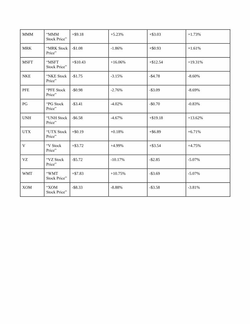
for 12 of the 28 Dow 30 companies. For example, the strategy performed extremely well with Walmart

stocks. It produced a markup (profit percentage) of about 10.75%, while the Buy and Hold strategy

performed 16% worse, with a markdown (loss percentage) of 5.068%. Other companies also generated a

good amount of profit with markups that are about 3% to 5% higher than their respective Buy and Hold

strategy markups.

4.3 Did it disprove the efficient market hypothesis?

The success rate of the new trading strategy suggests that the EMH could be disproved by

developing systems that would be able to process much larger sets of online data. The hypothesis does not

take into account new technologies that track the daily behavior and activities of people. The fact that a

success rate of 43% can be achieved with such a minimal amount of data suggests that it would be possible

to make more accurate predictions through large data sets. The more precise predictions, in turn, would

help us take advantage of the corresponding market fluctuations before it consumes the data and adjusts

itself accordingly. Therefore, with access to large streams of data that contain information about shareholder

and consumer interests (such as real time Google data of search terms that are related to the products and

services of a company), current and future technologies have a good chance of disproving the EMH.

4.4 Evaluation

The new trading strategy outperformed the Buy and Hold strategy for 43% of the tested Dow 30

companies. However, the success rate could be increased if we could eliminate additional factors that

increase noise in the data collected. For example, the following could be used to decrease noisy data:

● More GSV samples containing search terms that are related to the different services and products

provided by the companies. This would enable us to understand the public’s reaction to major

events involving the companies. For example, if a device manufactured by a company starts to

malfunction for most users, search terms related to the device will increase.

● More detailed GSV data. The current range of the index (0 – 100) conceals a lot of details about

the data. The same index value could be assigned to search volumes that are several million

numbers of searches apart.

● More accurate GSV data sets. Daily data has the potential to increase the efficiency of the strategy,

because the neural network usually performs better when it is trained with more detailed sets.

Instead of avoiding the use of daily GSV samples, a method could be implemented to remove the

discrepancies that come with concatenating GSV data sets. Or we could try to find other Google

resources to retrieve GSV data instead of using the Google Trends interface.

● More data included from additional sources such as financial news sources or social media sites

like Twitter.

5. Conclusion

We have described a computational procedure for relating GSVs to percent changes in trade

volumes for given assets on the Dow 30 that is potentially scalable to other assets beyond the scope of the

backtesting performed herein. While the results of our trading strategy are not conclusive enough to

warrant a rejection of the EMH, within the context of the Dow 30 over the time period between 1/1/2012

and 1/1/2017, the success ratio of 43% over the Buy and Hold trading strategy is nonetheless potentially

significant and should be researched further.

6. References ▪ Bao W, Yue J, Rao Y (2017) A deep learning framework for financial time series using

stacked autoencoders and long-short term memory. PLoS ONE12(7): e0180944.

https://doi.org/10.1371/journal.pone.0180944

▪ Bengio, Y., Frasconi, P., & Simard, P. (1993). The problem of learning long-term

dependencies in recurrent networks. IEEE International Conference on Neural Networks.

doi:10.1109/icnn.1993.298725

▪ Carlson, B. (2015). Buy and hold investing works, even when it looks like it's not. Retrieved

November 03, 2017, from http://www.businessinsider.com/buy-and-hold-investing-works-

2015-7

▪ Challet, Damien & Hadj Ayed Ahmed, Bel. (2013). Predicting Financial Markets with

Google Trends and Not so Random Keywords. SSRN Electronic Journal. .

10.2139/ssrn.2310621.

▪ Egmont-Petersen, M., Ridder, D. D., & Handels, H. (2002). Image processing with neural

networks—a review. Pattern Recognition, 35(10), 2279-2301. doi:10.1016/s0031-

3203(01)00178-9

▪ Fama, E. F. (1970). Efficient Capital Markets: A Review of Theory and Empirical Work. The

Journal of Finance, 25(2), 383. doi:10.2307/2325486

▪ Gers, F., & Schmidhuber, E. (2001). LSTM recurrent networks learn simple context-free and

context-sensitive languages. IEEE Transactions on Neural Networks, 12(6), 1333-1340.

doi:10.1109/72.963769

▪ Graves, A., & Schmidhuber, J. (2005). Framewise phoneme classification with bidirectional

LSTM and other neural network architectures. Neural Networks, 18(5-6), 602-610.

doi:10.1016/j.neunet.2005.06.042

▪ Hochreiter, Sepp & Schmidhuber, Jürgen. (1997). Long Short-term Memory. Neural

computation. 9. 1735-80. 10.1162/neco.1997.9.8.1735.

▪ Nath, T. (2015). Investing Basics: What Is The Efficient Market Hypothesis, and What Are

Its Shortcomings? Retrieved November 03, 2017, from

http://www.nasdaq.com/article/investing-basics-what-is-the-efficient-market-hypothesis-and-

what-are-its-shortcomings-cm530860

▪ Pasini A. Artificial neural networks for small dataset analysis. Journal of Thoracic Disease.

2015;7(5):953-960. doi:10.3978/j.issn.2072-1439.2015.04.61.

▪ Rogers, S. (2016). What is Google Trends data — and what does it mean? Retrieved October

29, 2017, from https://medium.com/google-news-lab/what-is-google-trends-data-and-what-

does-it-mean-b48f07342ee8

▪ Rouse, M. (2014). What is Information Age? - Definition from WhatIs.com. Retrieved

February 05, 2018, from http://searchcio.techtarget.com/definition/Information-Age

▪ Van Bergen, J. (2011). Efficient Market Hypothesis: Is The Stock Market Efficient?

Retrieved November 03, 2017, from

https://www.forbes.com/sites/investopedia/2011/01/12/efficient-market-hypothesis-is-the-

stock-market-efficient/#3c02cdc576a6

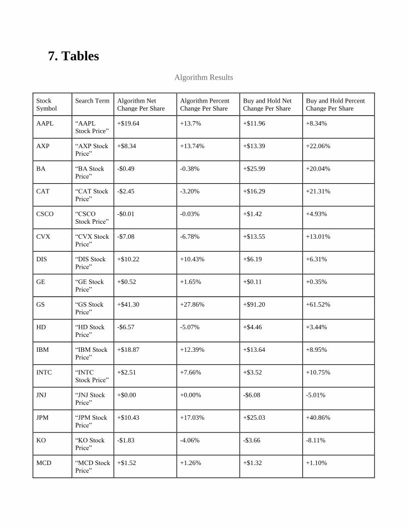
7. Tables

Algorithm Results

Stock

Symbol

Search Term Algorithm Net

Change Per Share

Algorithm Percent

Change Per Share

Buy and Hold Net

Change Per Share

Buy and Hold Percent

Change Per Share

AAPL “AAPL

Stock Price”

+$19.64 +13.7% +$11.96 +8.34%

AXP “AXP Stock

Price”

+$8.34 +13.74% +$13.39 +22.06%

BA “BA Stock

Price”

-$0.49 -0.38% +$25.99 +20.04%

CAT “CAT Stock

Price”

-$2.45 -3.20% +$16.29 +21.31%

CSCO “CSCO

Stock Price”

-$0.01 -0.03% +$1.42 +4.93%

CVX “CVX Stock

Price”

-$7.08 -6.78% +$13.55 +13.01%

DIS “DIS Stock

Price”

+$10.22 +10.43% +$6.19 +6.31%

GE “GE Stock

Price”

+$0.52 +1.65% +$0.11 +0.35%

GS “GS Stock

Price”

+$41.30 +27.86% +$91.20 +61.52%

HD “HD Stock

Price”

-$6.57 -5.07% +$4.46 +3.44%

IBM “IBM Stock

Price”

+$18.87 +12.39% +$13.64 +8.95%

INTC “INTC

Stock Price”

+$2.51 +7.66% +$3.52 +10.75%

JNJ “JNJ Stock

Price”

+$0.00 +0.00% -$6.08 -5.01%

JPM “JPM Stock

Price”

+$10.43 +17.03% +$25.03 +40.86%

KO “KO Stock

Price”

-$1.83 -4.06% -$3.66 -8.11%

MCD “MCD Stock

Price”

+$1.52 +1.26% +$1.32 +1.10%

MMM “MMM

Stock Price”

+$9.18 +5.23% +$3.03 +1.73%

MRK “MRK Stock

Price”

-$1.08 -1.86% +$0.93 +1.61%

MSFT “MSFT

Stock Price”

+$10.43 +16.06% +$12.54 +19.31%

NKE “NKE Stock

Price”

-$1.75 -3.15% -$4.78 -8.60%

PFE “PFE Stock

Price”

-$0.98 -2.76% -$3.09 -8.69%

PG “PG Stock

Price”

-$3.41 -4.02% -$0.70 -0.83%

UNH “UNH Stock

Price”

-$6.58 -4.67% +$19.18 +13.62%

UTX “UTX Stock

Price”

+$0.19 +0.18% +$6.89 +6.71%

V “V Stock

Price”

+$3.72 +4.99% +$3.54 +4.75%

VZ “VZ Stock

Price”

-$5.72 -10.17% -$2.85 -5.07%

WMT “WMT

Stock Price”

+$7.83 +10.75% -$3.69 -5.07%

XOM “XOM

Stock Price”

-$8.33 -8.88% -$3.58 -3.81%

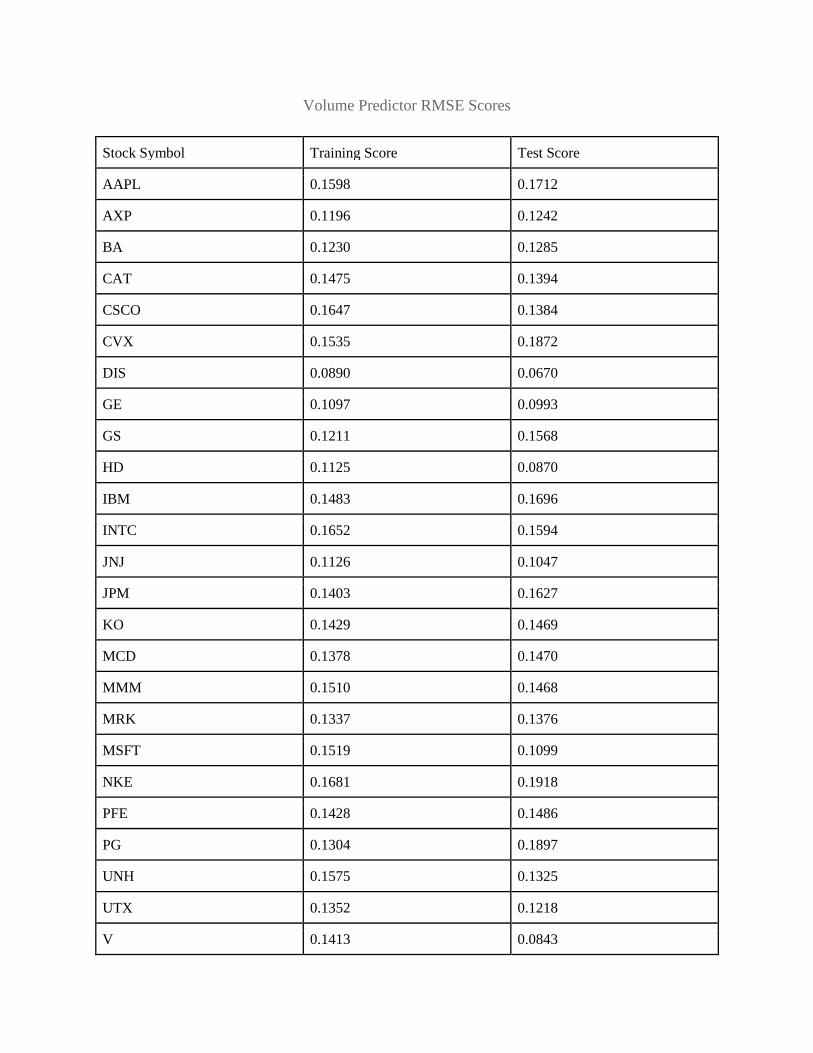
Volume Predictor RMSE Scores

Stock Symbol Training Score Test Score

AAPL 0.1598 0.1712

AXP 0.1196 0.1242

BA 0.1230 0.1285

CAT 0.1475 0.1394

CSCO 0.1647 0.1384

CVX 0.1535 0.1872

DIS 0.0890 0.0670

GE 0.1097 0.0993

GS 0.1211 0.1568

HD 0.1125 0.0870

IBM 0.1483 0.1696

INTC 0.1652 0.1594

JNJ 0.1126 0.1047

JPM 0.1403 0.1627

KO 0.1429 0.1469

MCD 0.1378 0.1470

MMM 0.1510 0.1468

MRK 0.1337 0.1376

MSFT 0.1519 0.1099

NKE 0.1681 0.1918

PFE 0.1428 0.1486

PG 0.1304 0.1897

UNH 0.1575 0.1325

UTX 0.1352 0.1218

V 0.1413 0.0843

VZ 0.0879 0.0483

WMT 0.0986 0.0746

XOM 0.1398 0.1908