Student 2013 Master Thesis, 30 ECTS Master’s Program in Economics, 60 ECTS

Trading Volume and Stock Return: Empirical Evidence for Asian Tiger Economies

Manex Yonis

Student 2013 Master Thesis, 30 ECTS Master’s Program in Economics, 60 ECTS

Acknowledgement

Thank you Kurt Brannas.

Student 2013 Master Thesis, 30 ECTS Master’s Program in Economics, 60 ECTS

Abstract

The relationship between returns, volatility and trading volume has interested

financial economists and analysts for the last four decades. This paper

investigates the contemporaneous and dynamic relationships between trading

volume, returns and volatility on Four Asian Tiger economies stock markets. I

also examine the causal relations among trading volume and returns between the

US and Tiger economies stock markets. I find a positive contemporaneous

relationship between absolute return and trading volume in the New York and

Tiger Economies stock markets using OLS and GMM estimator. Using MA-

GARCH (1, 1) model, trading volume has a statistically significant positive

effect on the conditional volatility of the markets, except South Korea. However,

my finding also confirms that the GARCH effects are still statistically significant

after considering trading volume in the variance equation. Moreover, the

selected EGARCH models, after the inclusion of contemporaneous trading

volume, attest the existence of a positive relationship between volatility and

trading volume in the US and Tiger Economies stock markets. A VAR(2) model

shows the existence of bi-causal relationship between return and trading volume

in the Singapore market whereas, there is no scope for improving the

predictability of returns by considering information flow in the form of trading

volume on the US, Hong Kong, Korea and Taiwan stock markets. Further,

impulse response and variance decomposition results confirm that the impact of

trading volume on price is insignificant in all the markets, indicating that trading

volume does not contain information to change returns. In contrast, except for

the case of Korea, there is a bi-causal relationship between volatility and volume

in the markets, explaining that volatility contains information to predict volume

and vice versa. Finally, the cross-country linkage, a result from a quad-variate

VAR(2) model, indicates that the US market return has significant spillover

effects on the Asian Tiger economies stock markets returns.

Key words: Trading volume, Stock return, Asian Tiger Economies, Cross-country linkage, GMM,

MA-GARCH, EGARCH, VAR, Impulse Response, Variance Decomposition.

Student 2013 Master Thesis, 30 ECTS Master’s Program in Economics, 60 ECTS

Table of Content

1. Introduction …………………………………………………………………. 1

2. Literature Review ……………………………………………………………… 5

3. Methodology …..…………………………………………………………….. 8

3.1. The Financial Time Series ...…………………………………. 8

3.2. Detrending Trading Volume ………………………………… 10

3.3. Conditional Heteroscedasticity …...………………………… 11

3.4. The Heteroscedasticity Process …………………………….. 12

3.5. The General ARCH and Heteroscedasticity Mixture

Model …….…………………………………………………… 13

3.6. Model Specification …………………………………………… 15

3.6.1. Contemporaneous Relationship

(OLS, GMM and MA-GARCH models) ……………… 15

3.6.2. Contemporaneous Volume as Stochastic

Mixing Variable, MA-GARCH (1, 1) …………………... 17

3.6.3. Contemporaneous Volume and Asymmetric

Response of Volatility (EGARCH) …...……………….. 18

3.6.4. Domestic and Cross-Country Dynamic Relationships,

bi-variate VAR (p) and quad-variate VAR(p) models ........... 20

3.6.5. Impulse Response Functions and Variance

Decompositions of Volume and Returns/Volatility ….…… 21

4. Data and Descriptive Analysis ……..………………………………………. 23

4.1. Data ...………………………………………………………… 23

4.2. The Financial Markets .………………………………………… 24

4.3. Summary Statistic ....…………………………………………. 26

4.4. Secular Trend and Detrending ..……………………………. 29

4.5. Stationarity Test for Return and Detrended Volume ………….... 30

4.6. Evidence for Conditional Heteroscedasticity ……..……………… 31

Student 2013 Master Thesis, 30 ECTS Master’s Program in Economics, 60 ECTS

5. Results ……………………………………………………………………. 34

5.1. Contemporaneous Relationship between Return and

Volume ……………………………………………………… 34

5.2. The Effect of Volume on Conditional Volatility ………………… 37

5.3. Trading Volume and Asymmetric Volatility ……………………. 38

5.4. Domestic Causal Relationship between Return,

Volatility and Volume …..………………………………………. 44

5.4.1. Granger Causality Test …...……………………………… 44

5.4.2. Estimated VAR(2) Parameters ...……..………………….. 47

5.4.3. Impulse Response and Variance Decomposition ………… 47

5.5. Cross-Country Causal Relationship among Return and

Trading Volume ……………………………………………… 49

6. Summary and Conclusion ….……………………………………………… 52

References ……………………………………………………………………… 53

Appendices ..…………………………………………………………………… 56

A. The pattern of the actual, fitted and residual series of

turnovers ……………………………………………………… 56

B. ARIMA (1, 1, 1) residuals autocorrelation ...………………….. 57

C. The markets turnover correlogram …………………………… 58

D. ARIMA (1, 1, 1) squared residuals correlogram ……….…… 60

E. Impulse response of volume on return and vice versa ...………… 61

F. Impulse response of volatility on volume and vice versa .……… 63

G. Variance decomposition of returns and volume due to

shocks in returns and volume …………………..……………… 66

1

1. Introduction

In recent financial studies, the linkage between return, volatility and trading volume is a central

issue as it, e.g., provides insights into the microstructure of financial markets. The price-volume

relationship is seen as “it is related to the role of information in price formation…” (Wiley and

Daigler, 1999 pp, 1). Trading volume is defined as the number of shares traded each day and is an

important indicator in technical analysis as it is used to measure the worth of stock price movement

either up or down (Abbondante, 2010).

Investors' motive to trade is solely dependent on their trading activity; it may be to speculate on

market information or portfolios diversification for risk sharing, or else the need for liquidity.

These different motives to trade are a result of processing different available information. In

consequence, trading volume may originate from any of the investors who may have different

information sets. As various studies reported, the information flow into the market is linked to the

trading volume and volatility (see, Gallant, Rossi and Tauchen, 1992). Thus, since the stock price

changes when new information arrives, there exists a relation between prices, volatility and trading

volumes (see, Lamoureux and Lastrapes, 1990 and He and Wang, 1995).

Moreover, numerous studies suggest that there are high correlations of returns across international

markets (see, e.g., Connolly and Wang, 2003). There is some overlapping trading period and

multiple listings of the same securities; thus, traders in one market draw inferences about the

market simply by focusing on price movements in other markets (King and Wadhwani, 1990).

Thus, it is logical to consider the fact that recent international financial markets process continuous

trading and uninterrupted transmission of information in their day to day trading activity, which is

reflected by returns, volume and volatility (Lee and Rui, 2002).

2

One of the leading hypotheses to explain the price-volume relationship, the mixture of distribution

hypothesis (MDH; Clark, 1973), suggests that price and volume are positively correlated. The

central proposition of this hypothesis claims that price and volume change simultaneously in

response to new information flow. The other popular hypothesis, sequential information arrival

hypothesis (SIAH), states that there is a positive bi-directional causal relationship between the

absolute values of price and trading volume. The model suggests a dynamic relationship whereby,

due to the sequential arrival of information, lagged trading volume may have the chance to predict

current absolute return and vise-versa (Darrat et al., 2003).

The contemporaneous and dynamic relationship between trading volume and stock returns have

been also the subject of a substantial stream of empirical studies. Lee and Rui (2002) found that

returns Granger cause trading volume in the US and Japanese markets. Besides, their result showed

that trading volume does not Granger cause returns in the US, UK and Japan markets. In their

study, De Medeiros and Doornik (2006), found a contemporaneous and dynamic relationship

between return volatility and trading volume by using data from the Brazilian market. In Flora and

Vouga’s (2007) study, trading volume was defined as the indicator of price movements. Mahajan

and Singh (2009), found a positive correlation between trading volume and volatility. Their study

also gave evidence of one-way causality from return to volume. More recently, the study by Choi

et al. (2012) found the significance of trading volume as a tool for predicting the volatility

dynamics of the Korean market by using GJR-GARCH and EGARCH models.

Significant efforts have been made, empirically and theoretically, on the phenomenon of stock

price and volume relationship. Although the majority of those findings have confirmed the

existence of positive contemporaneous relationship between trading volume and returns, the study

of different stock markets have given mixed results about the causal return-volume relationship.

3

Following the work of Lamoureux and Lastrapes (1990), there are also ongoing studies on if the

introduction of trading volume as an exogenous variable in the conditional heteroscedasticity

equation reduces volatility persistence. However, the studies are not consistence. Hence, the

relationship still remains a very interesting field for investigation in a different set of financial

markets with different perspectives.

The basic objective of this paper, therefore, is to study the relationship between return, volatility

and trading volume from two directions: First, the contemporaneous and dynamic relationships of

return, volume and volatility on Four Asian Tiger economies’ stock markets. Second, given recent

interest in return and volume spillover from one market to another market, this paper examines

causal relations among trading volume and returns between the US and Tiger economies’ stock

markets. The US market is considered as a proxy for developed markets.

The Four Asian Tigers, mostly refer to the economies of Hong Kong, South Korea, Singapore and

Taiwan. They are also called the Newly Industrialized Economies (NIEs). The last three decades,

due to reform processes to liberalize their financial markets and inflow of huge capital, witnessed

the takeoff of Tiger economies. The stock markets of the Tiger economies have relatively low

levels of regional linkage compared to the integration they have with developed markets (see, e.g.,

Soyoung Kim et al, 2008). More importantly, for my personal motivation, the information flow

and the institutional frameworks in these markets are different from those in the developed stock

markets.

This paper, therefore, contributes to the growing literature, and renders insight about the

microstructure of the stock markets by asking three research questions. First, does trading volume

contain information to change stock returns and volatility? Second, how stock markets react on

4

the arrival of new information due to trade commencement? Third, how asymmetric volatility and

volume affect the stock price change?

The following four points are considered significant in discussing the price-volume relationship in

Asian Tiger economies. First, it gives a better understanding of the microstructure of the stock

markets. Second, it demonstrates the rate of information flow to the market and how the

information is disseminated and how it influences stock return by applying linear regression

models (using OLS and GMM estimators), MA-GARCH models, and bi-variate VAR models. The

GARCH model specifies a symmetric volatility response to news; hence, third, the paper uses

exponential GARCH models to give new insight in the asymmetric effects of volatility, including

trading volume, and their impact on stock returns. Finally, it helps investors to have insight about

international cross-country stock return and trading volume co-movement by discussing quad-

variate VAR models.

5

2. Literature Review

Previous researches on stock markets were mainly focused on the stock return correlation among

different markets. However, the topic on the relationship between trading volume and stock returns

fascinated financial economists over the past three decades, and it has long been the subject of

empirical research. Karpoff (1987) discussed why it is important to study the stock price–volume

relationship by pointing out four important reasons.

First, the stock price-volume relationship provides insight into the structure of financial markets

that can describe how information is disseminated in the markets. Second, the price-volume

relationship is of great significance for event studies that use a combination of stock returns and

volume data to draw inferences. Third, it is an integral part of the empirical distribution of

speculative prices. And forth, it can provide insight into future markets (Karpoff, 1987).

Researchers like Clark (1973), Epps (1976) and Harris (1986) explain the price-volume relation as

positively correlated; because the variance of the price change on a single transaction is conditional

upon the volume of the transaction. Such a theoretical explanation is called the mixture of

distribution hypothesis (MDH). According to this hypothesis, the relationship is due to the joint

dependence of price and volume on an underlying common mixing variable, called the rate of

information flow to the market. This implies that whenever new information flows into the market,

the stock price and volume respond simultaneously. Thus, new equilibrium is established without

the occurrence of transitional equilibrium.

The other theoretical explanation, which is called the sequential information arrival hypothesis

(SIAH), labels the existence of a positive bi-directional causal relationship between absolute

values of price and trading volume. According to Copeland (1976) and Jennings et al. (1981),

6

unlike the MDH, new information that enter into the market disseminates to one market participant

at a time, implying that final equilibrium is established after a sequence of transitional equilibria

has occurred. Thus, such an argument suggests that lagged trading volume may have a predictive

power for current absolute price and vice-versa.

Regarding a relationship between volatility and volume, Lamoureux and Lastrapes (1990) argue

that volume has a positive effect on conditional volatility. According to their result, the inclusion

of trading volume in the conditional volatility vanishes the ARCH and GARCH effects. This

implies that past residuals and lagged volatility do not contribute much information regarding the

conditional variance of a return when volume is included. They argue that trading volume can be

a good proxy of information flow into the market. In general, the work of Lamoureux and Lastrapes

confirms that the GARCH effect may be a result of time dependence in the rate of information

arrival to the market for individual stocks returns.

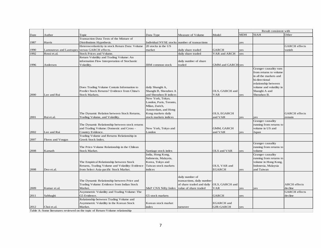
Thought the literature that study the price-volume relation is within the frameworks of MDH and

SIAH, recent empirical works use different econometric models and approaches to address the vast

area of the topic. However, different empirical studies give different results for different datasets.

Besides, several measures of volume were applied during the investigations of the return-volume

relation. In the following table, some studies are listed with the type of data set, kind of measure

of volume and kind of model that they applied, and the result.

7

MDH SIAH Other

1987 Harris

Transaction Data Tests of the Mixture of

Distributions Hypothesis. Individual NYSE stocks number of transactions yes

1990 Lamoureux and Lastrapes

Heteroscedasticity in stock Return Data: Volume

versus GARCH effects.

20 stocks in the US

market daily share traded GARCH yes

GARCH effects

vanish

1992 Rossi et.al. Stock Prices and Volume. daily share traded VAR and ARCH yes

1996 Andersen

Return Volatility and Trading Volume: An

information Flow Interpretation of Stochastic

Volatility. IBM common stock

daily number of share

traded GMM and GARCH yes

2000 Lee and Rui

Does Trading Volume Contain Information to

Predict Stock Returns? Evidence from China's

Stock Markets.

daily Shanghi A,

Shanghi B, Shenzhen A

and Shenzhen B indices

OLS, GARCH and

VAR yes

Granger causality runs

from returns to volume

in all the markets and

bi-directional

relationship between

volume and volatility in

Shanghi A and

Shenzhen B.

2001 Rui et.al.

The Dynamic Relation between Stock Returns,

Trading Volume, and Volatility.

New York, Tokyo,

London, Paris, Toronto,

Milan, Zurich,

Amsterdam, and Hong

Kong markets daily

stock markets indices

OLS, EGARCH

and VAR yes yes

GARCH effects

remain

2002 Lee and Rui

The Dynamic Relationship between stock returns

and Trading Volume: Domestic and Cross -

Country Evidence.

New York, Tokyo and

London

GMM, GARCH

and VAR yes

Granger causality

running from returns to

volume in US and

Japan

2007 Floros and Vougas

Trading Volume and Returns Relationship in

Greek Stock Index.

2008 Kamath

The Price-Volume Relationship in the Chilean

Stock Market. Santiago stock index OLS and VAR yes

Granger causality

running from returns to

volume

2008 Deo et.al.

The Empirical Relationship between Stock

Returns, Trading Volume and Volatility: Evidence

from Select Asia-pacific Stock Market.

India, Hong Kong,

Indonesia, Malaysia,

Korea, Tokyo and

Taiwan stock markets

indices

OLS, VAR and

EGARCH yes

Granger causality

running from returns to

volume in Hong Kong,

Indonesia, Malaysia

and Taiwan

2009 Kumar et.al.

The Dynamic Relationship between Price and

Trading Volume: Evidence from Indian Stock

Market. S&P CNX Nifty Index

daily number of

transactions, daily number

of share traded and daily

value of share traded

OLS, GARCH and

VAR yes yes

ARCH effects

decline

2011 Sabbaghi

Asymmetric Volatility and Trading Volume: The

G5 Evidence. G5 stock markets GARCH yes

GARCH effects

decline

2012 Choi et.al.

Relationship between Trading Volume and

Asymmetric Volatility in the Korean Stock

Market.

Korean stock market

index turnover

EGARCH and

GJR-GARCH yes

Table A: Some literatures reviewed on the topic of Return-Volume relationship

Result consistent with

Date Author Topic Data Type Measure of Volume Model

8

3. Methodology

3.1. The Financial Time Series

Financial time series analysis is concerned with a sequence of observations on financial data

obtained in a fixed period of time. According to Tsay (2005), financial time series analysis differs

from other time series analyses because the financial theory and its empirical time series contain

an element of complex dynamic system with high volatility and a great amount of noise (Tsay,

2005). The uncertainty and noise make the series exhibit some statistical regularity and fact. One

of the well accepted facts that most financial data series exhibit is the non-stationarity of the series.

Non-stationary time series has time varying mean and /or variance. Stationary time series, unlike

the non-stationary ones, have a time-invariant means, variances, and auto-covariances.

2

;

t t j j

t t j j

t t j jt

E x E x

var x var x

cov x x

A study related to the linkage between stock return, trading volume and volatility has to be done

by using an appropriate model. Before modeling any relationship, the non-stationarity of the data

series must be tested. For the purpose of this study, therefore, each market index is tested for the

presence of unit roots using the approach proposed by Dickey and Fuller (ADF, 1979, 1981) and

of stationarity using the approach proposed by Kwiatkowski, Phillips, Schmidt and Shin (KPSS,

1992).

9

A. Augmented Dickey-Fuller (ADF) test:

The general ADF unit root test is based on the following regression:

1 1 1 ....t t t p t p tY t Y Y Y (1)

where tY is a time series with trend decomposition, t is the time trend, α is a constant, β is the

coefficient on a time trend and p the lag order of the autoregressive process. The number of

augmenting lags (p) is determined by minimizing the Akaike Information Criterion (AIC). The

null hypothesis is that the series yt needs to be differenced or detrended to make it stationary can

be rejected if γ statistically significant with negative sign.

B. KPSS:

The KPSS test is proposed by Kwiatkowski, Phillips, Schmidt, and Shin in 1992. The previous

ADF unit root test is for the null hypothesis that a time series yt is I(1). But, the KPSS test is used

for testing a null hypothesis that an observable time series is stationary around a deterministic

trend.

1

t t t t

t t t

y

u

(2)

where t is constant or constant plus time trend, ut is I(0) and may be heteroscedastic. The null

hypothesis that yt is I(0) is formulated as H0 : σ2

e = 0. The KPSS test statistic is the Lagrange

multiplier (LM) or score statistic for testing σ2e = 0 against the alternative that σ2

e > 0 and is given

by:

10

2 2

1

T

t

tM SL

where tS is the partial sum of the error terms of a regression of yt that defined as 1

t

t j

j

S

and σ2

is an estimate of the long-run variance of ut.

3.2. Detrending Trading Volume

The other basic thing is that the stock price and the trading volume have different characteristics

of non-stationarity; if any. Therefore, the required treatment to induce stationarity may differ. A

series of raw trading volume has features of both linear and nonlinear time trends and experiences

slow and gradual changes in some statistical property of it (e.g., Gallant et al., 1992). It is

documented that trading volume is strongly autocorrelated unlike that of stock returns (see Wang

and Lo, 2000). This suggests a deterministic non-stationarity in trading volume. This paper will

check if the trading volume in the dataset has a trend and if there is deterministic non-stationarity,

proper methodology is conducted to induce stationarity. Most empirical studies of volume use

some form of detrending to induce stationarity (see, e.g., Lee and Rui, 2002, Wang and Lo, 2000).

Therefore, in order to detrend the series, I regress it on a deterministic function of time. To allow

for a linear and as well as a nonlinear trend, as suggested by Lee and Rui (2002), I define a

quadratic time trend equation:

2

t tV t t (3)

where Vt describes raw trading volume at time t, while t and t2 represent linear and quadratic time

trends, respectively. The detrended trading volumes, therefore, are the residuals. Unlike turnover,

11

stock price is characterized by stochastic non-stationarity and stationarity can be induced by

differencing.

3.3. Conditional Heteroscedasticity

The term heteroscedasticity refers to change in variance. Volatility modeling has been a fascinating

topic in financial markets studies, and risk is a central future of financial economics. However, the

methods of measuring and forecasting risk are hardly simple for time series analysis.

Financial time series are serially dependent, and this dependence is manifested by a decay of

correlation between a value at time t and t + h as h increases. The old fashioned view, in the process

of modeling financial time series dynamics that can measure the serial dependence, is

autocorrelation. These characteristics of decaying among the corresponding autocorrelations has

usually been related to long-memories in volatility (Rodriguez and Ruiz, 2005). Hence, conditional

heteroscedasticity is revealed if squared or absolute time series values are autocorrelated.

Conditional variance in asset returns varies systematically over the trading day. In line with this,

return volatility is viewed as a stochastic process which usually representing the underlying

variance. The explanation behind the conditional time varying volatility can be captured by the

idea that returns on assets are generated from a mixture of distributions in which the stochastic

mixing variable is considered to be the rate of daily information arrival into the market. Thus, in

asset return analysis, the observed heteroscedasticity is defined by the rate of information flow

arrival.

The second moment analysis introduced by Engle (1982) has been presented a good fit for many

financial return time series. The ARCH (Autoregressive Conditional Heteroscedasticity) process

12

of Engle (1982) allows the conditional variance to change over time as a function of past errors

and is able to let volatility shocks persist over time.

3.4. The Heteroscedasticity Process

Let ѱ is the information available up to and including time t-1. And, let {ɛt} be a discrete-time real

valued stochastic process generated by

½

1 2

 

~ 0, 1

, , , , )(

t t t

t t t

t t t t

z h

z iidN E z V z

h h x b

where ht is a time varying and non-negative function of the information set at time t-1, x is a vector

of predetermined variables and b is a vector of parameters. By definition, ɛt is serially uncorrelated

with mean zero, but with a time varying conditional variance ht. Even though, this can be defined

in a variety of contexts, conditional heteroscedasticity can be modeled by specifying the

conditional distribution of the errors be the innovation process in a dynamic linear regression

model:

1

~ 0, .| ( )

t t

t t t

y

N h

The original form of Engle (1982) linear ARCH model makes the conditional variance linear in

lagged values of second moment error terms (ɛ2t = z2

t ht ) by defining

2

0

1

 p

t i t i

i

h

13

The ARCH process allows the conditional variance to change over time as a function of past errors

while leaving the unconditional variance constant. The generalized autoregressive conditional

heteroscedasticity (GARCH) model, which was proposed by Bollerslev in 1986, has been a

preferred measure of volatility. Unlike ARCH, the GARCH process has a conditional variance that

changes over time as a function of past deviation from the mean and squared disturbance term.

The Generalized ARCH specification allows volatility shocks to persist over time and can be

extended to include other effects on the conditional variance. This persistence explains that returns

exhibit non-normality and volatility clustering (Fama, 1965). The GARCH specification can be

expressed by:

2

0

1 1

 p q

t i t i j t j

i j

h h

3.5. The General ARCH and Heteroscedasticity Mixture Model

Economic models that can explain the observed autoregressive conditional heteroscedasticity

phenomenon are not easy to find. Asking a question, what are the factors for the source of ARCH

effects in stock return series, can be a starting point for many empirical analysis.

In contemporary financial markets, a series of activities take place daily. Every single event

generates new relevant information that can facilitate a change in asset price, which is

accompanied by above average trading activity in the market. Accordingly, daily returns adjust to

a new equilibrium. Many studies documented that the possible presence of ARCH is based upon

the hypothesis that daily returns are generated by a mixture of distributions, in which the rate of

arrival of daily information flow is a stochastic mixing variable (see, Lamoureux and Lastrapes,

1990).

14

Lamoureux and Lastrapes (1990) relate the persistence of ARCH effects in stock returns to the

mixture of distribution hypothesis and suggest that conditional volatility persistence may reflect

serial correlation in the rate of information arrival. They discuss the theoretical process by which

ARCH may capture the serial correlation of the mixing variables, i.e. the rate of information

arrival, as follows: let ѱit denotes the Ith intra-day equilibrium price increment in day t. This implies

that the daily price increment, ɛt, is given by

1

tn

it

i

t

(4)

The number of events on day t is captured by a random variable, nt. Since the mixture hypothesis

basically assumes that the number of events occurring each day is stochastic, nt is the mixing

variable that represents the stochastic rate at which new information enters into the market. Thus,

εt is drawn from a mixture of distribution, where the variance of each distribution depends upon

information arrival time. Note, equation (4) implies that daily returns are generated by a stochastic

process, where ɛt is subordinate to ѱt, and nt is the directing variable (Lamoureux and Lastrapes,

1990).

At this point, if, ѱit ~ iid ( E(ѱit )=0, V(ѱit )=σ2) and the number of events occurring every day is

sufficiently large, then applying Central Limit Theorem leads

2 ~ 0, t tt n N n

The GARCH effect may be a result of time dependence in the rate of evolution of intraday

equilibrium returns. Lamoureux and Lastrapes (1990), to clarify the above argument, assume that

the number of events on day t are serially correlated. This correlation can be expressed as follows:

15

1

i t i

p

t t

i

n k n

In the above AR (p) model, k represents a constant and the error term ( t ) is white noise. An

autoregressive structure of 1

i t i

p

i

n

lets shocks in the mixing variable to persist. Let now define

2( | )t t tE n .

Consequently, if the mixture model is valid, then

2( ) ( )t t ttvar n E n

2

t tn

2

1

( )i t i

p

t t

i

k n

2 2

1

1

)p

t ti t

i

k

Note, the above equation explicitly defines the conditional deviation of the daily price change

from its mean as a function of its lagged value and a white noise error term. That means, the

equation captures a volatility persistence that can be picked by estimating a GARCH model.

16

3.6. Model Specification

To explain the possibly relationship between return, volatility and trading volume in the Tiger

Economies’ stock market indices, consider a stochastic vector time series {Rt} of the return at t of

a stock market index. Let {ɛt} be a discrete-time real valued stochastic process generated by

½  t t tz h

where {zt} is iid random variable with mean zero and unit variance and ѱt-1 is the information

available up to and including time t-1. After take away the serial dependence from the stock returns

first moment, a MA (1) process of the mean return is defined by

2

1

 

1

| (0, )

t t t

t

t t

t

t N

R

(5)

where μt is the conditional mean of Rt, based upon all past information.

3.6.1. Contemporaneous Relationship

One of the purposes of this study is to consider the contemporaneous relation between asset returns

and volume. In particular, to account for whether the positive contemporaneous relationship

between trading volume and stock return still exists, I apply three different proposed models.

Initially, I consider the relationship using a standard Ordinary List Square (OLS) regression

method as proposed by Smirlock and Starks (1988) and Brailsford (1994). Thus, I begin by

estimating the following equation:

0 1 2t tt t tV R uRD (6)

17

where tV is the daily trading volume, tR is the daily return and tD is a dummy variable, where

tD =1 if tR <0 and tD =0 if tR >=0. The estimates of 1 and 2 measure the relationship between

the return and volume, however, from different perspectives. The former measures irrespectively

of the direction of the return but the later permits asymmetry in the relationship.

For further testing of the contemporaneous relationship, I apply a multivariate model, proposed

by Lee and Rui (2002) and Vougas and Floros (2007), which is defined by

0 1 2 3

0 1 2

1 1

1 23

t t t t t

t t t t t

R V V R

V R V V u

(7)

The parameters of the equation are estimated using Generalized Method of Moments (GMM). This

estimation process, primarily, avoids simultaneity bias and gives consistent estimates of the

heteroscedasticity and autocorrelation. Moreover, it is a kind of robust estimator which does not

require information of the exact distribution of errors. Since the estimation process requires a list

of instruments, I use lagged values of volume and stock return and/or volatility.

Lastly, after controlling for non-normality of the error distribution, I estimate the following MA-

GARCH (1, 1) model, where volume is included in the mean equation. This model tests whether

the contemporaneous relationship between return and trading volume remains after considering

heteroscedasticity in the process. .

2

0 1 1

 

1

t

t t t t

t th

V

h

R

(8)

18

where Vt denotes volume and  

t is conditional mean return. The ARCH term,2

1t provides

information about volatility clustering and the GARCH term,2

1th is the lagged variance. The

persistence of volatility is measured by 1( ) .

3.6.2. Contemporaneous Volume as Stochastic Mixing Variable

According to the mixture distribution hypothesis (MDH), the variance of the price change in a

single transaction is conditional on the arrival of information into the market, which represents the

stochastic mixing variable. However, the stochastic rate at which information flows in the market

is unobserved. Thus, trading volume can be a proxy for the information flow into the market (see,

Lamoureux and Lastrapes, 1990). This stochastic process of stock returns can be estimated by a

GARCH model with a trading volume parameter in the variance equation. Generalized ARCH (1,

1) has been found to be a parsimonious and easy representation of the conditional variance that

adequately fit many economic time series (Bollerslev, 1987). To examine the effect of volume on

conditional volatility and re-examine whether the exogenous variable, trading volume, in the

conditional variance equation reduces the persistence of GARCH effects, I, therefore, select the

simple GARCH (1, 1) specification to be estimated for each stock and it can be given by:

1| ( , ) (0, )t t t tV N h ,

2

0 1 1 1t t t th h V (9)

The above model parameterized the conditional variance as a function of past squared innovation,

the lagged conditional variance, and the contemporaneous trading volume. Here, volume is added

as a proxy for the stochastic variable and, γ should be positive in order to comply with MDH

19

(Lamoureux and Lastrapes, 1990). Further, α1 and β measure the ARCH and GARCH effects,

respectively; and the persistence of volatility is measured by the sum of (α1 + β). According to

Lamoureux and Lastrapes, the sum becomes negligible, when the mixing variable, trading volume,

explains the presence of GARCH effects.

3.6.3. Contemporaneous Volume and Asymmetric Response of Volatility

Though the GARCH model responds to good and bad news, it does not capture leverage effects or

information asymmetry. Well documented empirical evidence suggests that large negative shocks

of asset returns are often followed by a larger increase in volatility than equally large positive

shocks (Brooks, 2008). Hence, conditional variance of asset return is asymmetric. To account for

the asymmetric response of volatility, I apply exponential GARCH model of Nelson (1991), which

extends GARCH with a log-specification form.

Traditionally, the process of modeling GARCH and its extensions are conducting with a normal

error distribution. However, studies have been done on GARCH models with non-normal error

distribution to sufficiently capture the heavy tails, skewness and leptokurtic characteristics of stock

return (see. e.g. Hansen, 1994, Liu and Hung (2010). Thus, particularly, I consider two different

scenarios of innovation distribution in the process of estimating the EGARCH model, Normal

distribution and Student t-distribution. The latter suggests t-distribution for error terms in order to

capture leptokurticity of returns (Bollerslev, 1987).

The following EGARCH (p, q) model is used to inspect the relationship between the trading

volume and conditional volatility by considering the asymmetric effect.

20

1

0

11

| |

mt jt i

t t

q p

i j k t

kt i t j

k

i j

ln h ln h Vh h

(10)

where α0, αi, γj, βk and ω are parameters to be estimated. The persistence of conditional variance

and leverage effect are measured by the parameters β and γ, respectively. Ideally, γ is expected to

be negative, implying that negative shocks generate greater volatility change than positive ones.

Moreover, ω should be a nonzero and positive parameter in order to have an information based

conditional variance model. The log of the conditional variance in the left side defines that the

leverage effect is exponential, which implies that no constraints on the parameters are needed to

impose in order to ensure non-negativity of the conditional variance.

3.6.4. Domestic and Cross-Country Dynamic Relationship

A significant concern, when it is about a dynamic context, is whether available information about

trading volume is a useful stream in the process of forecasting asset price change and volatility.

Simply, testing causality is a better way of understanding a stock market microstructure. Thus, this

paper empirically examines not only contemporaneous but also dynamic relationship to investigate

causality between trading volume and volatility (return). The empirical procedure is thus, based

on the premise that the future cannot cause the present or the past.

The following bi-variate VAR model of order p is used to test for Granger causality (Granger,

1969) in which returns and volume are used as endogenous variables.

0

1 1

1

0

1

t i t i j t j

t i t i j

p p

rt

i j

p p

vj t

i j

t

R R V

V V R

(11)

21

The above VAR model is re-estimated with square of stock returns instead of return levels to

analyze the dynamic effect of volatility on trading volume and vice versa. Parameters, i and j

from the first equation, represent the effect of lagged return and lagged volume on the present

return. Similarly, parameters i and j from the second equation represent the effect of lagged

volume and lagged return on the present volume, respectively. If j ≠ 0, lagged volume has

influence and then we say volume Granger cause return ( ... ...V GC R ) and vice versa if j ≠ 0 (

... ....R GC V ). Note that the null hypotheses are all equal to zero and F-statistic is used to test it.

Moreover, if j and j are significant, there exists bi-directional causality between returns and

volumes. Beside the Granger Causality test and parameter estimates from VAR, I also consider

the dynamic relationship through impulse response function and variance decomposition

sequences.

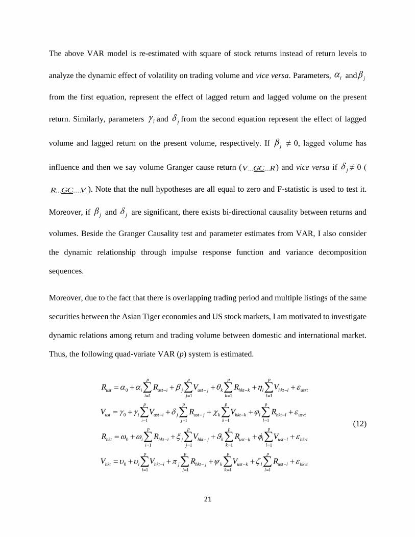
Moreover, due to the fact that there is overlapping trading period and multiple listings of the same

securities between the Asian Tiger economies and US stock markets, I am motivated to investigate

dynamic relations among return and trading volume between domestic and international market.

Thus, the following quad-variate VAR (p) system is estimated.

1 1 1 1

1 1 1

1

0

0

1

0

1

1

p p p p

k l usrt

i j k l

p p p p

k l usvt

i j k l

p p

k l hkr

ust i ust i j ust j hkt k hkt l

ust i ust i j ust j hkt k hkt l

hkt i hkt i j hkt j ust k u l

k

s t

l

t

i

R R V R V

V V R V R

R R V R V

1

1 1 1 1

0

p p

j

p

hkt i hkt i j hkt j

p p p

k l hkvt

i j k l

ust k ust lV V R V R

(12)

22

where Rus and Vus are return and volume for the US market, which is good enough to be a proxy

for developed markets and, Rhk and Vhk are return and volume for the Hong Kong market which

belongs to the other Tiger Economies’ market when the system is conducted for the same.

3.6.5. Impulse Response Functions and Variance Decomposition of Returns and Volume

The dynamic change of joint dependency is immediately not considerable. Thus, impulse response

functions (IRFs) trace the effects of one standard deviation shock to one of the innovations on the

whole process over time. I use it in this paper to analyze the effect of a shock on the residual of

return ( rt ) on volume and vice versa.

Variance decomposition sequences are an alternative way of analyzing the dynamic structure of a

VAR model. It decomposes the uncertainty in an endogenous variable into the component shocks

to the endogenous variables in the VAR. The function enables to capture system wide shocks and

the impact between the system variable.

23

4. Data and Descriptive Analysis

4.1. Data

My dataset comprises daily closing stock price indices and corresponding trading volume series

of the Hong Kong (HKEX), Korea (KRX), Singapore (SGX), Taiwan (TWSE) and lastly, USA

(NYSE) stock markets. The indices include Hang Seng index for Hong Kong (HNGKNGI), Korea

composite index for Korea (KORCOMP), Straits Times index for Singapore (FSTSTI), Taiwan

weighted index for Taiwan (TAIWGHT) and NYSE composite index for USA (NYSEALL). Data

on daily closing stock price index values is obtained from DATASTREAM database.

A number of measures of volume have been proposed by different studies on trading activity of

financial markets (W. Lo and J. Wang, 2001). Such as,

a. Total number of shares traded as a measure of volume (Gallent, Rossi and Tauchen, 1992)

b. Aggregate turnover as a measure of volume (W. Lo and J. Wang, 2001)

c. Individual share volume as a measure of volume (Lamoureux and Lastrapes (1990)

Though, the dissimilarity of existing measures for volume suggest the inconsistency in the

measurement of trading volume. I used turnover by volume as a daily trading volume of the stock

market as suggested by W. Lo and J. Wang (2001).

Except NYSE, data on daily number of shares traded are obtained from Yahoo Finance. The data

of daily volume (turnover by volume) for all stocks is taken from DATASTREAM. The dataset

covers the period extending from Dec 31, 2002 to Dec 31, 2012, for a total of around 2600

observations.

24

4.2. The Financial Markets

According to the report of Heritage Foundation, Hong Kong has been in the leading position in

terms of economic freedom for the last 18 consecutive years (1995-2012). Hong Kong, as a city,

is a well-functioning international financial center. The stock exchange of Honk Kong was

established in 1891. Based on market capitalization, as of Jul 2013, the stock market of Hong Kong

ranked at the sixth and second largest in the world and Asia, respectively. The stock market has

1575 listed companies, with a market capitalization of HK$ 21,509.4 billion, as of Jul 2013.

The financial market in Korea has grown rapidly for the past two decades. One of the divisions

under the Korean Exchange is the Stock Market Division. This division, before Jane 27, 2005, was

called the Korea Stock Exchange (KSE); where the Korea Exchange was formed from the merger

of three former exchanges: the Korea Stock Exchange, Korea Securities Dealers Association

Automated Quotation, and Korea Future exchange. The Stock Exchange (KSE) was formally

established in 1956. As of Nov 2010, KSE ranked seventeenth, ninth and forth in the global market

based on market capitalization, number of listed companies and turnover velocity respectively.

KSE has 777 listed companies with KRW$ 1,140 trillion market capitalization as of the end of

2010. The exchange market is the one among the markets that shown strong resilience and market

performance after the recent global financial crises.

In 1965, after the independence from Malaysia, Singapore took steps to be a financial center. Since

then, the financial market is the world’s fastest-growing market for private wealth management

and become a global financial center. According to the 2012 report on benchmarking global city

competitiveness, US 1.8 trillion assets were under management in Singapore, which makes the

country wealth management hub of Asia with largest institutional investor base. The Singapore

25

exchange market (SGX) is considered as a truly international exchange compared to other

developed and emerging markets due to a higher number of international listed companies. The

report on SGX on Aug 2012 stated that the market has 775 listed companies with US$ 720 billion

market capitalization, out of which 40% were non-Singapore based. The existing and the most

globally recognized benchmark index and market barometer for the SGX is Straits Times Index,

renovated once again on Jan 2008. It comprises top 30 Mainboard companies listed on the SGX

which is ranked by market capitalization.

Back to the history, in 1949 one major policy initiative was taken, which is shared by both the

Taiwanese government and the Chinese Communist Party. It was a land reform, “land-to-the-

tiller”. Ironically, the movement led in Taiwan to the establishment of the Taiwan Stock Exchange

(TWSE). Formally, the stock exchange was established on 1961 and operation begins in 1962. As

of the end of 2012, TWSE has 809 listed companies with a market capitalization of NTD 21,352

billion. The ratio of market capitalization to GDP was 152.11% on the same ending year, 2012.

Following the 1997 Asian financial crises, all tiger economies countries introduced reforms to

further develop and deepen financial markets. Subsequently, these economies had strengthened

current accounts and banking systems and builds in foreign reserves (C. L. Lee and S. Takagi,

2013). After more resilient financial system for consecutive years, however, the recent global

economic crises brought these four countries financial markets to a halt, though in a limited way.

In a more general way, as a legacy from the lessons learned during the Asian crises in 1997, these

countries escaped, relatively unhurt, from the recent crises and recovered faster than other regions

due to the deep work on strengthening their current account and improving the regulatory oversight

(IMF, 2009).

26

4.3. Summary Statistic

The continuously compounded daily stock return series for each market is obtained by taking the

first logarithm difference of daily closing price.

Rt = 100*log (Pt / Pt-1)

where Pt is the closing price at time t. Table 1 reports the descriptive statistics for these returns

and the corresponding volume. All the markets are indicating a high level of daily return

fluctuation, considering the high values of all the markets standard deviation. Except Taiwan, the

standard deviation of Tiger economies’ market is higher than US market. Turning to individual

markets, I find a more volatile market in Hong Kong and a less volatile one in Taiwan as measured

by the standard deviation of 1.61 and 1.33 respectively.

All the markets, except Hong Kong, are left-skewed. It indicates, in these markets, that large

negative stock returns are more common than large positive returns. The kurtosis values for all

market return series are greater than three and thus, the indices have higher peaks. Besides, the

Jarque-Bera statistics reject the null hypothesis of normality for the markets. Overall, the

descriptive statistics suggest that the return of all markets is volatile and non-normally distributed.

I discussed the gross characteristics of volume by considering the total share traded and turnover

index of the markets that are under consideration. Over the entire sample, in both data, the

deviation from its mean of a volume is high in Hong Kong and low in Taiwan. The analyses on

trading volumes indicate positive skewness and greater than three kurtosis for the markets. This

suggests that the distribution is skewed to the right and also leptokurtic. Basically, the summary

27

statistics for trading volume show that the volume of the markets is volatile, and the null hypothesis

of normality is rejected.

Table 1

Descriptive statistics for daily returns, raw volume and turnover over 2003 to 2012 Return

Market Obs. Mean Median Max Min Sts.dev skewness Kurtosis Jarque-Bera

NYSE 2609 0.020083 0.052796 11.52575 -10.23206 1.354029 -0.399 13.3488

11711.5932

(0.000)

HKEX 2609 0.034042 0 13.40681 -13.58202 1.569322 0.0336 12.7651

10366.57

(0.000)

KRX 2609 0.04437 0.05203 11.28435 -11.172 1.464389 -0.5013 8.954

3962.9869

(0.000)

SGX 2609 0.047517 0.071749 9.788895 -9.108143 1.372498 -0.2296 7.9335

2668.7826

(0.000)

TWSE 2609 0.020993 0.011005 6.52462 -6.912347 1.326018 -0.3646 6.1247

1119.1898

(0.000)

Volume (Share traded)

Market Obs.

Mean

%

Median

%

Max

%

Min

%

Sts.dev

% skewness Kurtosis Jarque-Bera

HKEX 2507 1.28E+07 1.24E+07 9.80E+07 - 1.04E+07 1.397576 7.597999

3024.535

(0.000)

KRX 2480 9242.542 3884 4.07E+06 1364 131122.76 26.4196 722.9202

53844624

(0.000)

SGX 2523 951401.21 651490 1.02E+07 - 1.13E+06 1.28472 5.846793

1545.994

(0.000)

TWSE 2476 37296.78 34954 115582 - 15056.91 1.097865 4.898651

869.2928

(0.000)

Volume (Turnover)

Market Obs.

Mean

%

Median

%

Max

%

Min

%

Sts.dev

% skewness Kurtosis Jarque-Bera

NYSE 2518 13265.67 13570 29646.76 2864.29 3780.975 0.201193 3.479491

41.10903

(0.000)

HKEX 2474 14012.55 12985.87 204330.2 708.06 10571.62 3.473173 47.92415

213014.6

(0.000)

KRX 2474 4112.183 3870.045 98487.06 88.94 2345.545 26.52792 1060.795

116000000

(0.000)

SGX 2514 46.76563 33.26 522.29 1.84 43.35997 2.819497 17.64412

25794.54

(0.000)

TWSE 2479 40.45987 37.86 116.31 13.69 14.09821 1.259396 5.333084

1217.56

(0.000)

28

Note that results from descriptive statistics of both measurements of the trading volume provide

similar explanation on the characteristics of volume.

The analysis on the possible lead-lag relationship between markets, which is done by calculating

a cross-correlogram of 4 lag for each the Tiger markets versus the New York market return, give

light that there may be an international return co-movement. As shown in Table 2, most of the

significant correlations are limited to first three lags. Mostly, the Tiger markets are positively

influenced by current day and yesterday’s return of the New York market.

Note that the Tiger economies and New York markets do not have a single overlap trading hour.

Thus, market adjustments cannot be completed within a day; instead, it can be done with at least

one lag. Consistently with this fact, interestingly, the table shows that yesterday’s influence from

New York returns is much stronger than current day’s impact on the Tiger markets; particularly,

it has a strong positive impact on Hong Kong. Finally and expectedly, there is an indication that

the Tiger economies stock markets have no significant influence on the New York market.

Table 2: Cross-correlations for Tiger economies stock return series Vs. US

lag/Lead

Markets -4 -3 -2 -1 0 1 2 3 4

vs. US

Hong

Kong

-0.0227 0.0232 0.0193 0.4241* 0.2715* -0.008 -0.0346 -0.0041 -0.0038

Korea -0.0305 0.0501* 0.0501* 0.3761* 0.2324* 0.0051 -0.0621 0.0008 -0.0005

Singapore -0.0124 -0.0031 0.0637* 0.3861* 0.3148* 0.0014 -0.0305 0.0185 -0.0161

Taiwan -0.0077 0.0446* 0.0545* 0.3809* 0.1694* 0.0082 -0.0094 -0.0135 0.0114

Note: * indicates significant correlations

29

4.4. Secular Trend and Detrending

Turnover cannot be negative. This is because, turnover is an asymmetric measure of trading

activity. Thus, logically, its distribution is skewed. Table 1 reports that the empirical distribution

of turnover is positively skewed. Moreover, the pattern of the turnover series of all the markets

have a trend pattern. The turnover of Hong Kong market was raised at a constant percentage

growth rate over the entire sample period. Even if there was a lot of short-run fluctuations, the

New York and Singapore market turnovers also show a slow growth during the beginning of the

sample period and then a decline pattern. In contrast, the other two markets’ turnovers, Korea and

Taiwan, are relatively constant through the entire sample period, though Taiwan shows a slight

decline during the end period of the dataset (see Appendix Figure A).

The turnover autocorrelation reveals that turnover is strongly autocorrelated unlike that of stock

return. More evidently, a correlogram shows autocorrelations that start at 71.5%, 67.7%, 27.4%,

65.7%, 83.5% for the US, Hong Kong, Korea, Singapore and Taiwan turnover index, respectively,

decaying very slowly to 54.5%, 54.3%, 18.9%, 43%, 59.2% at lag 10 (see, Appendix B). Thus,

turnover is highly persistence in these markets and the slow pattern of decaying recommend some

kind of long memory in turnover. Accordingly, it may require treatment to induce stationarity. To

do so, I regress it on a deterministic function of time; i.e. I detrend the series.

30

Table 3: Parameter estimates for linear and nonlinear trend in trading volume

Turnover of α β γ Adj. R. sq. (%)

NYSE 1294545 592.3304 -0.326478 45.7844

(77.74103) (20.08691) (-29.82519)

HKEX -386427.1 2691.623 -0.759345 38.8801

(-7.754151) (30.4888) (-23.17957)

KRX 538958.4 -286.3969 0.108335 5.3989

(-39.09191) (-11.72199) (11.94878)

SGX 607.4217 9.674559 -0.003768 19.4685

(2.612935) (23.49274) (-24.64432)

TWSE 3720.586 0.99684 -0.000429 2.7532

(44.31012) (6.70922) (-7.795745)

Notes: t-statistics are in parenthesis

From Table 3, the coefficients of both linear and non-linear time trend terms are statistically

significant at 1% level. Therefore, in this study, I will employ turnover (afterwards: trading

volume) that are free from linear and non-linear time trend for all concerned markets. These

detrended trading volumes are represented by the residuals of equation (3). Besides, the pattern of

the actual, fitted and residual series of the estimated equation are presented (see Figure A in

Appendix).

4.5. Stationarity Test for Return and Detrended Volume

Table 4 presents the result of ADF and KPSS test for the return and detrended volume series.

According to the ADF tests, I reject the null hypothesis which requires difference or detrending of

a data; thus, stock return and detrended volume series are clearly stationary in all the markets.

Similarly, based on the asymptotic critical values of KPSS, I cannot reject the null hypothesis that

affirm the stationarity of the series of return and detrended volume. Generally, since both tests

approved, the stock return and detrended volume data are clearly stationary. With this setup,

31

therefore, I confidently proceed to the analysis of returns and volume relationship without risk of

spurious correlation.

Table 4: Stationery test for stock returns and trading volumes

Stock Return

Market Lag(s) Critical Value (1%) ADF Bandwidth

Asymptotic

Critical Value

(1%) KPSS

NYSE 17 -3.432681 -11.98075* 10 0.739000 0.149299*

HKEX 17 -3.432676 -13.97897* 3 0.739000 0.112337*

KRX 0 -3.432665 -50.11661* 13 0.739000 0.126868*

SGX 16 -3.432680 -11.18102* 6 0.739000 0.134564*

TWSE 15 -3.432679 -12.27738* 1 0.739000 0.106840*

Trading Volume (Detrended Turnover)

Market Lag(s) Critical Value (1%) ADF Bandwidth

Asymptotic

Critical Value

(1%) KPSS

NYSE 20 -3.437385 -4.016710* 33 0.739000 0.052049*

HKEX 14 -3.435344 -4.707270* 35 0.739000 0.375014*

KRX 9 -3.434202 -4.929731* 33 0.739000 0.171123*

SGX 9 -3.433865 -7.268967* 35 0.739000 0.244263*

TWSE 10 -3.433857 -6.048337* 38 0.739000 0.179244*

Note: * indicates statistically significant at the 1% level and lag is chosen based on AIC

4.6. Evidence for Conditional Heteroscedasticity

Before dealing with the conditional heteroscedasticity process, I need to check whether ARCH is

necessary for the data in concern. I estimate appropriate ARIMA models for each market price

index. One of the most important benefits of ARIMA is, it helps to pick a right model that can fit

the data I concerned and its ability to remove local linear trends in the data.

Based on AICs, ARIMA (1, 1, 1) model is found to be a good fit for all the markets stock price

indices. The residual diagnostic test of correlogram, which I basically focused on is ACF and

PACF, has no any significant lags, indicating ARIMA (1, 1, 1) is a good model to represent the

data (see Appendix B).

32

Though ARIMA model is best linear method to forecast the series, it does not respond for new

information, implying the necessity of nonlinear model that reflects new changes. So; does ARCH

is necessary for the series in order to model variance in the series? Figure 1b shows the graphical

appearance of the squared residual that attests the presence of volatility clustering in the US and

Tiger Economies’ stock returns. Moreover, as shown in ACF and PACF plots of the markets’

squared residuals, ACF die out and PACF cut off after some lags, confirming that the residuals are

not independent (see Appendix D). Overall, there is, evidently dependency in returns’ second order

moments that traditionally are captured by ARCH.

Figure 1a: Indices of the New York and Tiger Economies stock Exchange

0

4,000

8,000

12,000

16,000

20,000

24,000

28,000

32,000

2003 2004 2005 2006 2007 2008 2009 2010 2011 2012

New York

Taiwan

Hong Kong

Singapore

Korea

33

Figure 1b: Squared residuals plot from ARIMA (1,1,1) model for the markets

0

20,000

40,000

60,000

80,000

100,000

120,000

140,000

03 04 05 06 07 08 09 10 11 12

New York

0

200,000

400,000

600,000

800,000

1,000,000

1,200,000

1,400,000

03 04 05 06 07 08 09 10 11 12

Hong Kong

0

1,000

2,000

3,000

4,000

5,000

03 04 05 06 07 08 09 10 11 12

South Korea

0

10,000

20,000

30,000

40,000

50,000

60,000

70,000

03 04 05 06 07 08 09 10 11 12

Taiwan

0

10,000

20,000

30,000

40,000

50,000

60,000

04 06 08 10 12

Singapore

34

5. Results

5.1. Contemporaneous Relationship between Return and Volume

In this section, I present the empirical results of models that are used to investigate the

contemporaneous relationship between return and trading volume. Table 5 shows estimation

results of OLS and GMM linear models, and GARCH model that includes volume in the mean

equation.

Section A of the table reports the OLS regression results of the estimates of 1 and 2 , which

measure the relationship between volume and return in different aspects. In all the markets the

estimates of α₁, with the exception of the case of Singapore (which is significant at the 5% level),

are positive and statistically significant at the 1% level. This implies that positive contemporaneous

relationship between trading volume and absolute return, irrespective of the asymmetric effect of

return, exists in the New York and Tiger Economies’ stock markets. Note that it is consistent with

previous findings on the topic (Smirlock and Starks, 1988 and Chen et al, 2001).

Table 5: Contemporaneous relationship between returns, trading volume and volatility

New York Hong Kong Korea Singapore Taiwan

Section A. OLS test of contemporaneous relationship: return and trading volume

α₀ -0.2622 -0.397 -0.0676 -0.2339 -0.1566

(-10.554)* (-16.326)* (-2.3697)** (-6.9483)* (-5.5697)*

α₁ 0.2844 0.376 0.0842 0.2107 0.2437

(11.923)* (19.83)* (3.4162)* (2.575)** (9.1182)*

α₂ 0.0227 -0.0168 -0.0424 0.1237 -0.1646

(0.8208) (-0.7506) (-1.5702) (1.6574)*** (-5.6223)*

35

Table 5: Continued

New York Hong Kong Korea Singapore Taiwan

Section B. GMM test of contemporaneous relationship: return and trading volume

α₀ 0.5908 0.83 0.0734 0.6022 -0.3487

(4.4303)* (5.9421)* (0.4238) (16.238)* (-0.9860)

α₁ 0.5537 0.903 0.1222 0.4498 2.3176

(3.4592)* (7.7686)* (3.0335)* (2.5911)* (3.7818)*

α₂ -0.203 -0.3641 -0.0676 -0.1752 -2.1412

(-2.9025)* (-5.3028)* (-1.7966)*** (-2.1041)** (-3.7392)*

α₃ 0.3252 0.2104 0.9323 0.2213 1.3678

(2.4638)** (1.7956)*** (5.7416)* (4.6096)* (3.7480)*

β₀ -0.9482 -0.4161 -4.2339 -0.2211 -1.5195

(-8.1665)* (-7.1638)* (-2.7992)* (-2.4620)** (-2.2567)**

β₁ 1.089 0.3738 4.003 0.286 1.5607

(9.1257)* (7.825)* (2.7222)* (2.4442)** (2.2480)**

β₂ 0.2886 0.3901 0.1401 0.4399 0.7502

(7.4206)* (10.437)* (2.1072)** (15.647)* (8.2327)*

β₃ 0.058 0.1543 0.0659 0.1402 0.0881

(2.2572)** (7.0615)* (1.7146)*** (3.6767)* (1.0111)

J-test 0.001 0.004 0.000 0.000 0.000

Section C. GARCH test of contemporaneous relationship: return and trading volume

θ 0.05422 0.0736 0.0966 -0.229 0.0733

(3.1953)* (3.2932)* (3.896)* (-10.212)* (2.9744)*

φ -0.06 0.0166 0.0152 0.0634 0.0567

(-4.1161)* (0.7435) (0.6757) (2.6059)* (2.5369)**

ω -0.0746 0.0118 0.006 -0.1977 0.123

(-4.1161)* (0.4756) (0.1946) (-12.27)* (5.9507)*

α₀ 0.0133 0.0141 0.0289 0.0216 0.024

(5.1093)* (3.5602)* (4.2908)* (4.4198)* (4.8235)*

α₁ 0.0807 0.0676 0.0834 0.0914 0.0736

(10.871)* (9.6474)* (10.025)* (9.1688)* (11.288)*

β 0.9091 0.9258 0.9026 0.8885 0.9135

(108.81) (120.03)* (97.28)* (76.825)* (117.67)*

36

Table 5: Continued

New York Hong Kong Korea Singapore Taiwan

Section D. GARCH test of contemporaneous relationship: trading volume and volatility

restricted, where γ = 0

α₁ 0.0804 0.0675 0.0834 0.0992 0.069

(11.163)* (9.6902)* (10.027)* (9.9097)* (10.929)*

β 0.9092 0.926 0.9027 0.8793 0.919

(111.79)* (120.65)* (97.307)* (77.428)* (121.95)*

α₁ + β 0.9896 0.9935 0.9861 0.9785 0.988

unrestricted, where γ in non-zero

θ 0.0012 0.0735 0.0983 -0.1864 0.0705

(0.0489) (3.2646)* (3.9575)* (-7.9764)* (2.8973)*

φ -0.066 0.0162 0.0158 0.0774 0.0655

(-2.7695)* (0.7389) (0.6981) (3.1387)* (2.9385)*

α₀ 0.7669 0.0369 0.0296 0.0438 0.0226

(50.936)* (5.1732)* (4.3344)* (6.0728)* (5.2617)*

α₁ 0.2773 0.0633 0.0833 0.1013 0.0562

(7.5299)* (9.0717)* (9.9927)* (9.0223)* (8.84)*

β 0.3441 0.9183 0.9025 0.8585 0.9304

(12.299)* (107.32)* (97.334)* (63.533)* (129.93)*

γ 0.2358 0.0336 0.0111 0.0276 0.0148

(12.916)* (4.7572)* (1.5127) (3.9565)* (5.637)*

α₁ + β 0.6214 0.9816 0.9858 0.9598 0.9866

Note: Vt is the standardized daily measure of volume. Dt is a dummy variable where Dt = 1 if rt <0,

and Dt = 0 if rt ≥ 0. *, ** and *** indicate statistically significant at the 1%, 5% and 10% level,

respectively.

In contrast, the estimates of α₂ that allow asymmetry in the relations are insignificant except in the

Taiwan and Singapore markets, which are shown to be statistically significant at the 1% and 10%

level, respectively. The value of α₂ in Singapore is negative and implies that the impact of an

upward return on trading volume is powerful than that of downward return, and vice-versa to

Taiwan.

37

Section B of the table reports the regression results where GMM estimator is employed. Whether

the system is over-identified, the process is tested by J-test. The test statistics of all the markets

are small, indicating that there exists a good fit of models to the data. The coefficients, α₁ and β₁

of all the markets, are positive and significant at the 1% level and 5% level, suggesting that there

is a positive contemporaneous relationship between absolute return and trading volume in the New

York and Tiger Economies’ stock markets. Evidently, the findings of this section are consistent

with MDH hypothesis. Interestingly, the value of α₂ is statistically significant in all the markets,

and it suggests that the lagged value of the volume contains information about returns.

Once again, section C of Table 5 reports findings from MA-GARCH (1, 1) models that include

trading volume in the mean equation. From the results, except in the case of Taiwan, coefficients

of volume are either non-positive or insignificant. Accordingly, after considering

heteroscedasticity in the process, there is evidence of positive contemporaneous relationship

between return and trading volume only in the Taiwan market (Since ω is positive and significant

at the 1% level). However, the GARCH models suggest that past innovation and volatility

persistence have a significant impact on daily stock return behavior of all the markets.

5.2. The Effect of Volume on Conditional Volatility

Estimation results of MA-GARCH (1, 1) models with an exogenous variable of trading volume in

the variance equation, while excluding the contemporaneous volume in the mean equation, are

presented in section D of Table 5. Initially, as a benchmark, the results of estimated coefficients

of the restricted variance model (excluding volume) are presented; and, as expected, there is strong

evidence that the daily stock returns of all the markets can be characterized by the GARCH model.

The volatility persistence in all markets returns, as measured by the sum of ARCH and GARCH

38

effects, is high and takes the value of p such that; 1 > p > 0.90, where p is the value of persistence.

This implies that the US and Tiger Economies’ stock returns have high persistence of shocks to

the volatility and are covariance stationary.

The unrestricted GARCH process tests whether trading volume be a proxy for the stochastic rate

at which information flows in the market. The reports show that, except South Korea, trading

volume has a statistically significant positive effect on the conditional volatility of all the markets,

indicating that contemporaneous volume significantly explains volatility. Thus, the results are

consistent with the MDH. In the other side of the mirror, however, the GARCH effects are still

statistically significant after considering trading volume in the variance equation. This means that

the arrival of information into the markets that conditioned the variance is not totally captured by

volume, though the volatility persistence in the markets indices has shown a moderate reduction

due to the inclusion of the exogenous trading volume variable. Note that the reduction is high in

the US daily stock return index.

In contrast with the argument given by Lamoureux and Lastrapes (1990), which claims an

important reduction and/or insignificant of ARCH and GARCH effects on conditional volatility

due to the inclusion of volume, the results show that the inclusion of volume does not appear to

eliminate the GARCH effects at all. Nevertheless, they are compatible with findings that trading

volume does not extract all information flow into the market (see, e.g., Chen et. al, 2001 and

Sabbaghi, 2011).

5.3. Trading Volume and Asymmetric Volatility

Table 6 presents the results of four different scenarios where trading volume is included in the

conditional asymmetric variance equation.

39

Table 6. Contemporaneous relationship between trading volume and volatility:

New York Hong Kong Korea Singapore Taiwan

Scenario A. EGARCH (1, 1) with normal distribution

θ 0.0382 0.0409 0.0526 -0.2069 0.0467

(2.3217)** (1.9201) (2.1989)** (-8.9249)* (1.996)**

φ -0.044 -0.0562 0.0266 0.0832 0.071

(-1.9279)*** (-3.0011)* (1.2173) (3.216)* (3.2012)*

α₀ -0.0884 0.3787 -0.0932 -0.1075 -0.066

(-8.1679)* (8.8586)* (-7.2782)* (-5.4744)* (-6.9771)*

α₁ 0.1143 0.1153 0.1436 0.1027 0.0931

(8.2569)* (3.035)* (8.8175)* (3.9177)* (7.4547)*

γ₁ -0.0978 -0.0962 -0.1441 -0.154 -0.0895

(-9.613)* (-3.8786)* (-10.789)* (-7.649)* (-11.205)*

β₁ 0.9837 -0.0379 0.96022 0.8861 0.9816

(474.71)* (-2.1767)** (208.6)* (67.05)* (387.47)

ω 0.0086 1.0622 0.0331 0.0452 0.0192

(2.2895)* (29.8182)* (5.4483)* (4.9519)* (11.848)*

AIC 2.8672 3.294 3.3253 2.6982 3.1948

SCI 2.8834 3.3104 3.3418 2.7177 3.2113

Q (12) (30.398)* (412.91)* (27.447)* (17.947) (13.812)

0.001 0000 0.004 0.083 0.244

ARCH (1) (12.007)* (0.7691) (7.3235)* (2.7486) (6.7187)*

0.0005 0.3805 0.0068 0.0973 0.0095

Scenario B. EGARCH (1, 1) with t-distribution

θ 0.0527 0.0512 0.0791 -0.1416 0.0366

(3.4111)* (2.452)** (3.4407)* (-6.9745)* (1.7184)***

φ -0.0443 -0.0561 0.0153 0.0628 -0.0119

(-2.0277) (-3.0211)* -0.6927 (2.5873)* (-0.7586)

α₀ -0.0911 0.4027 -0.0956 -0.1098 1.0984

(-6.4306)* (7.4538)* (-5.6281)* (-4.2355)* (-6.8682)*

40

Table 6: Continued

New York Hong Kong Korea Singapore Taiwan

α₁ 0.1155 0.0958 0.1423 0.1068 0.0495

(6.1984)* (2.1209)** (6.5016)* (2.9909)* (1.4691)

γ₁ -0.1031 -0.1151 -0.1493 -0.1129 -0.0984

(-7.6724)* (-3.8036)* (-9.0214)* (-4.2839)* (-3.5274)*

β₁ 0.9864 -0.054 0.9615 0.9159 -0.6735

(371.70)* (-3.1458)* (171.84)* (55.757)* (-13.708)*

ω 0.0093 1.0739 0.0312 0.0315 0.5929

(1.9017)*** (27.234)* (4.3109)* (3.2027)* (10.357)*

AIC 2.8387 3.2868 3.3125 2.6745 3.2671

SCI 2.8573 3.3056 3.3314 2.6967 3.2859

Q (12) (26.785)* (421.62)* (26.165)* (15.897) (447.5)

0.005 0000 0.006 0.145 0000

ARCH (1) (11.330)* (1.4679) (6.5221) (1.147) (4.3243)

0.0008 0.2257 0.0107 0.2842 0.0376

Scenario C. EGARCH (2, 2) with normal distribution

θ 0.0383 0.0571 0.0503 -0.2072 0.041

(2.4142)** (2.5899)* (2.1592)** (-9.0108)* (1.8962)***

φ -0.0525 0.0155 0.016 0.0773 0.0685

(-3.0463)* (0.7304) (0.8009) (2.9106)* (3.802)*

α₀ -0.1349 -0.1148 -0.1273 -0.1858 -0.0957

(-7.6946)* (-4.4002)* (-6.2777)* (-5.2834)* (-6.0102)*

α₁ -0.1483 0.0594 -0.019 0.0181 -0.1097

(-4.2605)* (1.8597)*** (-0.5219) (0.4379) (-3.2483)*

α₂ 0.3225 0.1309 0.2166 0.1658 0.246

(8.8344)* (3.9994)* (5.7655)* (3.7194)* -6.7904

γ₁ -0.1333 -0.1561 -0.1961 -0.2167 -0.1212

(-8.179)* (-8.66)* (-10.227)* (-8.3247)* (-9.1139)*

β₁ 0.66 0.1669 0.5619 0.2291 0.7182

(5.502)* (2.8971)* (4.7276)* (2.4961)** (5.3726)*

β₂ 0.3129 0.7514 0.3821 0.5994 0.2544

(2.6451)* (13.1995)* (3.3073)* (6.5208)* (1.9313)***

ω 0.018 0.1019 0.046 0.0826 0.0268

(3.4233)* (9.3291)* (5.5425)* (5.7168)* (8.1505)*

AIC 2.8492 3.2641 3.3173 2.6892 3.1841

SCI 2.8701 3.2853 3.3385 2.7142 3.2053

41

Table 6: Continued

New York Hong Kong Korea Singapore Taiwan

Q (12) (12.815) (28.938)* (24.208)* (18.734) (9.4558)

0.306 0.002 0.012 0.066 0.58

ARCH (1) (0.3552) (10.63)* (0.4263) (2.0198) (0.1241)

0.5512 0.0011 0.5138 0.1553 0.7246

Scenario D. EGARCH (2, 2) with t-distribution

θ 0.0556 0.056 0.0771 -0.1473 0.0252

(3.7197)* (2.6701)* (3.4402)* (-7.2148)* (1.2082)

φ -0.049 -0.0396 0.0085 0.0635 -0.0089

(-2.7947)* (-2.0545)** (0.4481) (2.554)** (-0.5984)

α₀ -0.1404 0.1281 -0.1275 -0.1884 1.1416

(-6.0934) (1.951)*** (-5.1101)* (-3.903)* (5.7039)*

α₁ -0.1557 0.1125 -0.082 0.0288 -0.0305

(-3.1696)* (2.4541)** (-1.7091)*** (0.4967) (-0.7585)

α₂ 0.3339 0.204 0.2732 0.1537 0.2574

(6.4999)* (3.9528)* (5.3676)* (2.6354)* (6.0185)*

γ₁ -0.1413 -0.1399 -0.1982 -0.1837 -0.1014

(-6.5182)* (-4.4531)* (-8.0024)* (-4.9301)* (-3.5708)*

β₁ 0.6841 -0.0376 0.6263 0.2637 -0.5797

(4.7126)* (-1.2817) (4.4549)* (1.6152) (-10.102)*

β₂ 0.2916 0.1902 0.3212 0.5866 -0.4519

(2.0368)** (4.2512)* (2.3491)** (3.7414)* (-8.6428)*

ω 0.0198 0.8926 0.0419 0.0701 0.7203

(2.7269)* (19.620)* (4.3057)* (4.0418)* (11.970)*

AIC 2.8249 3.2779 3.3029 2.6699 3.2546

SCI 2.848 3.3014 3.3264 2.6977 3.2781

Q (12) (11.133) (236.84)* (23.179) (18.515) (100.23)*

0.432 0000 0.017 0.07 0000

ARCH (1) (0.2548) (0.0579) (0.2624) (1.3234) (3.1524)

0.6137 0.8098 0.6085 0.25 0.0758

Note: *, ** and *** indicate statistically significant at the 1%, 5% and 10% level, respectively.

Q (12) is Ljung-Box statistic test for serial correlations up to a 12th lag length in the squared

standardized residuals. ARCH (1) is a Heteroscedasticity test of which tests the effect at 1st order

lagged squared residual.

42

Scenario A and B report estimated coefficients of an EGARCH (1, 1) model with Gaussian-Normal

distribution and t-distribution, respectively; and with moving average mean specification. In all

cases, the results show that trading volume effect coefficients are significantly positive and

asymmetry effect coefficients are significantly negative. This implies that the inclusion of volume

as a proxy of information arrival lets the process capture the leverage effect.

Scenario C and D report results of estimated coefficients of a high-order EGARCH model with

moving average mean specification, and with Gaussian-Normal distribution and t-distribution,

respectively. There is evidence of statistically significant positive effect of volume and negative

effect of asymmetry on the conditional variance from both innovation distributions for an

EGARCH (2, 2) model.

The accuracy of each model, to which market the model is specified, is studied by using

information criteria and residual-based diagnostic tests. The former includes Akaike’s Information

Criterion (AIC) and Schwarz Information Criterion and the latter includes serial correlation and

heteroscedasticity test. For the US market, the lower values of AIC and SCI are found from

EGARCH (2, 2) with t-distribution and; in this model, neither Ljung-box Q (12) and ARCH (1)

are significant at the 1% level, implying accepting no serial correlation and ARCH effect

hypothesis. Thus, after taking into account the contemporaneous trading volume effect in the

variance equation, the New York market return seem to be better characterized by EGARCH (2,

2) model with moving average mean specification and with t-distribution.

By comparing its AIC and SCI values, in the case of Hong Kong, EGARCH (2, 2) model with

normal distribution is superior to the rest of the model specifications. In this specification,

however, the Ljung-box Q (12) and ARCH (1) are significant, indicating that there is serial

43

correlation up to a 12th lag length in the squared standardized residuals, and ARCH effects at 1st

ordered lagged of squared residual. When the innovation distribution switched to t-distribution,

the ARCH effect disappears. However, both model specifications are consistent with MDH that

contemporaneous volume significantly explains conditional volatility even after consideration of

the asymmetric effect.

Based on the information criteria and, the Ljung-box Q (12) and ARCH (1) tests, which are

insignificant, EGARCH (2, 2) model with t-distribution fits the return series of Korea market in a

better way. As well, the model is sufficient for measuring the effects of information arrival to the

market, when trading volume is considered in the process.

Scenario D is a manifest that the best model with an exogenous variable in the variance equation,

in the case of Singapore, is the one with higher order EGARCH, i.e. EGARCH (2, 2), t-distribution,

and moving average mean specification. Neither of residual-based diagnostic tests is significant at

the 1% level and, AIC and SCI values are lower than the comparable model specifications.

The result from Table 6 shows that an EGARCH (2, 2) model with Gaussian distribution is better

to capture the behavior of the Taiwan stock return series, when trading volume is included in the

process. Among the rest of model specifications, the model has lower AIC and SCI values and

there is evidence of insignificant Ljung-box (12) and ARCH (1) tests, indicating no serial

correlation and ARCH effects on the squared standardized residual series.

Overall, the selected exponential GARCH models, after the inclusion of contemporaneous trading

volume, attest the existence of a positive relationship between volatility and trading volume in the

US and Tiger Economies’ stock markets. Therefore, the results are describing that trading volume

affects the rate at which information flow in the market, complying with MDH.

44

5.4. Domestic Causal Relationship between Return, Volatility and Volume

5.4.1. Granger Causality Test

A bi-variate VAR(2) model is chosen based on AIC and SCI to investigate the dynamic

relationship between return, volume and volatility. Table 7 presents the Granger causality test and

the corresponding significance levels of estimated parameters.

Table 7: Dynamic relationship between return, volume and volatility

Causality Direction New York Hong Kong Korea Singapore Taiwan

Panel A: Causal relationship among return and volume

F-test 0.5701 0.3878 0.0332 4.6524 0.391

(0.5655) (06786) (0.9673) (0.0096)* (0.6764)

α₁ -0.0961 -0.0228 0.0267 0.1339 0.0526

(-4.7985)* (-1.1331) (1.3235) (5.9290)* (2.5843)*

α₂ -0.053 0.0104 -0.024 0.1652 0.006

(-2.62634)* (0.5148) (-1.1891) (7.3057)* (0.2959)

β₁ 0.0114 0.0267 0.0017 -0.0302 0.0461

(0.3446) (0.7042) (0.0548) (-1.0404) (0.8827)

β₂ 0.0216 0.0033 0.0072 -0.054 -0.0372

(0.6611) (0.0861) (0.2309) (-1.8793)*** (-0.7202)

F-test 38 1.6494 1.6018 4.1658 36.5626

(0.0000)* (0.1924) (0.2017) (0.0155)** (0.0000)*

γ₁ 0.4278 0.4021 0.2001 0.4507 0.5916

(21.745)* (20.498)* (10.090)* (19.9001)* (30.388)*

γ₂ 0.1828 0.2254 0.177 0.1574 0.2879

(9.4032)* (11.489)* (8.9282)* (7.0098)* (14.939)*

δ₁ -0.1005 -0.0135 0.0195 -0.0449 0.0625

(-8.4229)* (-1.2939) (1.5182) (-2.5441)** (8.2471)*

δ₂ -0.0373 -0.0136 0.0116 -0.0175 0.0149

(-3.0964)* (-1.3040) (0.9081) (-0.9890) (1.9568)**

45

Table 7: Continued

Causality Direction New York Hong Kong Korea Singapore Taiwan

Panel B: Causal relationship between volatility and trading volume

F-test 6.7236 9.4235 0.6415 4.4855 3.863

(0.0012)* (0.0000)* (0.5266) (0.0114)** (0.0211)**

α₁ 0.1203 0.2675 0.1414 0.1939 0.1027

(6.4513)* (13.199)* (7.2104)* (8.8055)* (5.1027)*

α₂ 0.3931 0.2519 0.2334 0.2665 0.1474

(21.025)* (12.385)* (11.892)* (12.098)* (7.3807)*

β₁ 0.5092 0.5483 0.0735 0.271 -0.3844

(3.6135)* (2.9184)* (0.5996) (2.6453)* (-2.5262)**

β₂ -0.181 0.2903 0.0966 -0.0215 0.4178

(-1.2914) (1.5534) (0.7888) (-0.2106) (2.7564)*

F-test 9.6465 13.5184 4.5038 2.956 8.3258

(0.0000)* (0.0000)* (0.0112)** (0.0523)*** (0.0002)*

γ₁ 0.4346 0.3719 0.1969 0.4594 0.6114

(21.783)* (18.165)* (9.9184)* (20.397)* (31.225)*

γ₂ 0.1666 0.2081 0.1743 0.1505 0.2769

(8.3962)* (10.220)* (8.7903)* (6.6940)* (14.191)*

δ₁ 0.0116 0.0091 0.0071 0.0047 0.0081

(4.38493)* (4.1150)* (2.2437)** (0.9614) (3.1447)*

δ₂ -0.0014 0.0037 0.0049 0.0093 -0.0075

(-0.5134) (1.6781) (1.5542) (1.9142)*** (-2.9259)*

Note: *, ** and *** indicate statistically significant at the 1%, 5% and 10% level, respectively.

The table shows that, at 5 % significant level, the null hypotheses that trading volume does not

Granger cause stock market returns of US, Hong Kong, Korea and Taiwan is accepted. This

implies that there is no scope for improving the predictability of returns by considering information

flow in the form of trading volume. Moreover, since the mixture distribution hypothesis describes

the existence of no causal effect from volume to return, this finding is consistence with the

46

hypothesis and studies like Gallant et al. (1992) and Lee and Rui (2000). However, it contradicts

with the sequential information arrival model of Copeland (1976) and Smirlock and Starks (1988)

that explains about the significant predictive power of trading volume for future returns.

In contrast, the null hypothesis that stock returns do not Granger cause trading volumes is rejected

in the US, Singapore and Taiwan markets but not in the case of Hong Kong and Korea markets.

This implies that returns in these three markets contain significant information for volume.

Moreover, note that there is a bi-causal relationship between return and trading volume in the

Singapore market which is an evidence that information arrives sequentially instead of

simultaneously in the market, and it is consistent with SIAH and Copeland (1976).

Table 7, also, presents the results whether trading volume proceeds stock returns volatility and/or

vice versa. Except in the case of Korea, there is a bi-causal relationship between volatility and

volume in the markets, explaining that volatility contains information to predict volume and vice

versa. This implies, thus, that information flow in the markets is indirectly through volatility which

can be seen as consistence with the mixture distributions hypothesis that uses trading volume as a

proxy for the stochastic mixing variable in the process of driving conditional volatility (see, Clark,

1973 and Lamoureux and Lastrapes, 1990). The null hypothesis, at a 5% significant level, that

volatility does not Granger cause trading volume is rejected for the Korea stock market, implying

that volatility helps to predict trading volume.

Overall, the Granger causality test results attest the difficulty of improving the predictability of

returns by including trading volume in the process of deriving stock prices of the Tiger Economies’

markets, except Singapore. Once more, the results confirm that the rate of information flow in the

47

Tiger Economies’ markets can be captured by trading volume indirectly through volatility, albeit

Korea is exceptional.

5.4.2. Estimated VAR(2) Parameters

Table 7 also presents the sign and magnitude effects of a return on trading volume and vice versa,

and volatility on trading volume and vice versa. The dynamic effects of the stock returns on trading

volume are significant and negative in the US and Singapore stock markets and positive in the

Taiwan stock market.

The dynamic effects of volatility on trading volume and vice versa are also examined. As shown

from table 7, trading volume is significantly and positively affected by one lag volatility in the US,

Hong Kong, Korea and Taiwan stock markets. Lag one trading volume has significant positive

effect on stock volatility in the US, Hong Kong and Singapore stock markets, whereas it has a

negative effect in the case of Taiwan. Interestingly, from both circumstances, when the lag effect

dissolves quickly from other stock markets, the sign of the lag effect is changed over time in the

Taiwan case.

5.4.3. Impulse Response (IRF) and Variance Decomposition (VDF)

The dynamic adjustments of reciprocal dependency are further examined by IRFs and VDFs. IRFs’

multi-graphs present the effect of one standard deviation (SD) shock on the innovation of return

on trading volume and vice versa (see, Figure in Appendix E). The graphs show that, except in the

case of Singapore, returns are not responding at all to one SD trading volume shock. Interestingly,

the Singapore stock market returns also do not respond immediately to an innovation shock on

volume; it responds after the 2nd day and dissolves gradually over time. In contrast, trading volume,

48

to one SD return shock, responds immediately and the dynamic effect declines gradually over time

in the US, Singapore and Taiwan stock markets. This implies that shocks to return have an impact

not only on the process of predicting the future dynamics of return but also on the process of

predicting the future dynamics of trading volume.

The US, Hong Kong and Singapore stock markets return volatility initially responds positively to

one SD trading volume shock and the effect of trading volume declines quickly in the US market

while it takes time to disappear from the Hong Kong and Singapore markets (see, Appendix F). In

the case of Taiwan, trading volume shock initially has a negative effect on the volatility of the

market, albeit the effect vanishes quickly.

A SD innovation shock from volatility has a positive effect on trading volume in all the markets.

With the exceptional case of South Korea where the dynamic effect of the return volatility

disappears in few days, the effect decays gradually over time in all the other markets.

Beside the IRFs that can provide economic significance for the dynamic relationship analysis,

VDFs are studied. The results are presented in Appendix G. The Figures show that any variation

in stock returns is almost 100%, explained by its own lagged returns in all the markets. This

implies, stock returns are highly autoregressive, meaning that change in returns is explained by

their own past shocks than trading volume.

It is evidently shown from the figures that, though, the variability of trading volume is mainly

explained by its own lagged shocks, the contribution of returns in explaining trading volume

increases gradually over time; for e.g. within ten days, it increases from 0.95% to 6.23%, from

5.01% to 7.77% and, from 2.39% to 10.9% in the US, Singapore and Taiwan markets, respectively.

The exceptional cases are Hong Kong and Korea where the contribution of returns in explaining

49

trading volume is less than 0.5% during the first ten days. This result provides strong evidence that

past return shocks can have information which helps to predict trading volume in these three

markets.

Overall, from IRFs and VDFs results, the impact of trading volume in the process of price

determination is insignificant in all the markets, indicating that trading volume does not contain

information to change returns. It contradicts with SIAH that explains about the significant

predictive power of trading volume for future returns. However, the stock returns contain

information to predict trading volume in the US, Singapore and Taiwan markets. Moreover, except

in the case of Korea market, shocks to trading volume contain information to predict not only the

future dynamics of volume but also the future dynamics of return volatility in the Tiger Economies’

and US markets.

5.5. Cross-Country Causal Relationship among Return and Trading Volume

Based on AIC and SCI criteria, lag two high order quad-variate VAR model is chosen to capture

the return and volume spillover effects across countries. Table 8 presents a result of a causal

relationship that exists between trading volume and return across countries.

The cross-country linkage indicates that the US market return, dominantly, has significant

spillover effects on the Asian Tiger economies’ stock markets returns. Specifically, there is a bi-

directional dynamic relationship between the US and South Korea and the US and Singapore stock

markets returns.

50

Table 8: International causal relationship between return and volume

US GC Hong Kong F-statistic Prob. Null hypothesis

Return → Return 328.85 (0.0000)* reject

Volume → Return 2.5832 (0.0758) accept

Return → Volume 2.2281 (0.1080) accept

Volume → Volume 15.0982 (0.0000)* reject

Return ← Return 0.6895 (0.5020) accept

Return ← Volume 0.5709 (0.5651) accept

Volume ← Return 6.4715 (0.0016)* reject

Volume ← Volume 0.34144 (0.7108) accept

US GC South Korea F-statistic Prob. Null hypothesis

Return → Return 218.73 (0.0000)* reject

Volume → Return 3.7285 (0.0242) accept

Return → Volume 0.9214 (0.3981) accept

Volume → Volume 0.7143 (0.4897) accept

Return ← Return 5.2642 (0.0052)** reject

Return ← Volume 0.0265 (0.9739) accept

Volume ← Return 1.4065 (0.2452) accept

Volume ← Volume 1.5930 (0.2035) accept

US GC Singapore F-statistic Prob. Null hypothesis

Return → Return 10756 (0.0000)* reject

Volume → Return 14.9729 (0.0000)* reject

Return → Volume 36.9735 (0.0000)* reject

Volume → Volume 12.5104 (0.0000)* reject

Return ← Return 8.8699 (0.0001)* reject

Return ← Volume 3.0945 (0.0456) accept

Volume ← Return 6.9879 (0.0010)* reject

Volume ← Volume 2.2373 (0.1072) accept

US GC Taiwan F-statistic Prob. Null hypothesis

Return → Return 210.07 (0.0000)* reject

Volume → Return 2.2735 (0.1032) accept

Return → Volume 38.6013 (0.0000)* reject

Volume → Volume 12.1813 (0.0000)* reject

Return ← Return 1.234 (0.2913) accept

Return ← Volume 1.0524 (0.3493) accept

Volume ← Return 3.2389 (0.0394) accept

Volume ← Volume 0.6625 (0.5157) accept

Note: * and ** indicate statistically significant at the 1% and 5% level, respectively.

51

Except in the case of South Korea, trading volume from US Granger Causes the trading volume

of all the Tiger economies’ stock markets, indicating the validity of the information contained in

the US trading volume for the Tiger economies’ stock markets trading volume. Thus, the US stock

market return Granger Causes not only return but also trading volume of the Singapore and Taiwan

stock markets.

There are also interesting results from the table: first, the US stock market information contained

in the form of return and volume has significant predictive power for the Singapore return and

trading volume. Second, the US trading volume is Granger Caused by the Hong Kong and

Singapore stock markets returns. Last, there are no spillover effects from the Taiwan market to the

US market in terms of return and trading volume.

Overall, I find that the US has significant impact on the Tiger Economies’ stock markets in terms

of return and trading volume spillover. This implies that the US stock returns and trading volume

have potential predictive power for price formation in Tiger Economies’ stock markets, which is

consistence with the result of Lee and Rui (2002) that ratified the significant influence of the US

market on a cross-country relationship.

52

6. Summary and Conclusion

In recent financial studies, the linkage between stock return, volatility and trading volume has

received considerable attention. Hence, I motivated to investigate the relationship from two

directions: First, the contemporaneous and dynamic relationships of return, volatility and volume

on Four Asian Tiger economies’ stock markets. Second, given recent interest in return and volume

spillover from one market to another market, this paper examines causal relations among trading

volume and returns between the US and Tiger economies’ stock markets.

The dataset comprises daily closing stock price indices and corresponding trading volume series

of the Hong Kong (HKEX), Korea (KRX), Singapore (SGX), Taiwan (TWSE) and lastly, USA

(NYSE) stock markets for the period extending from Dec 31, 2002 to Dec 31 2012. Besides, I used

turnover by volume as a daily trading volume of the stock markets.

The finding suggests that there is a positive contemporaneous relationship between absolute return

and trading volume in the New York and Tiger Economies’ stock markets, implying that the stock

return and trading volume response simultaneously for the arrival of new information into the

markets. Moreover, except South Korea, trading volume has a statistically significant positive

effect on the conditional volatility of all the markets, thereby suggesting that the arrival of

information into the markets, due to trade commencement, is instrumental in bringing about the

returns movement. However, unlike the finding of Lamoureux and Lastrapes (1990), my finding

confirms that the GARCH effects are still statistically significant after considering trading volume

in the variance equation.

The results from the estimated coefficients of a high-order EGARCH models provide an evidence

of statistically significant positive effect of volume and negative effect of asymmetry on the

53

conditional variance. Therefore, the above results are describing that trading volume affects the

rate at which information flow in the markets, complying with mixing distribution hypothesis.

My empirical procedures also test whether trading volume proceeds returns and volatility or vice

versa. The results confirm that trading volume does not Granger cause stock market returns of US,

Hong Kong, Korea and Taiwan, implying no scope for improving the predictability of returns by

considering information flow in the form of trading volume. Moreover, further investigations on

the dynamic adjustments of reciprocal dependency by Impulse response functions and Variance

decomposition functions confirm that the impact of trading volume in the process of price

determination is insignificant in all the markets, indicating that trading volume does not contain

information to change returns. However, except in the case of South Korea, there is a bi-causal

relationship between volatility and volume in the markets, explaining that volatility contains

information to predict volume and vice versa.

The paper, secondly, investigates the dynamic relations among return and trading volume between

domestic and international market. I find that the US has a significant impact on the Tiger

Economies’ stock markets in terms of return and trading volume spillover. This implies that the

US stock return and trading volume have potential predictive power for price formation in Tiger

Economies’ stock markets, which is consistence with the result of Lee and Rui (2002) that ratified

the significant influence of the US market on a cross-country relationship.

54

References

Abbondante P. (2010). " Trading Volume and Stock Indices: A Test of Technical Analysis"

American Journal of Economics and Business Administration 2, 287-292.

Andersen. (1996). "Return Volatility and Trading Volume: An Information Flow Interpretation

of Stochastic Volatility", Journal of Finance 51, 169-204.

Bollerslev T. (1986). " Generalized Autoregressive Conditional Heteroscedasticity"

Journal of Econometrics 105, 5-26

Bollerslev T. (1987). "A Conditional Heteroscedasticity Time Series Model for Speculative

Prices and Rate of Return" Review of Economics and Statistics 69, 542-547.

Brailsford T. J. (1994). "The Empirical Relationship between Trading Volume, Returns

and Volatility", Accounting and Finance 36, 89-111.

Brooks C. (2008). "Introductory Econometrics for Finance", Reading, Cambridge University Press,

Edition 2.

Chen G.-M, Firth M. & Rui O. (2001). "The Dynamic Relation between Stock Returns,

Trading Volume and Volatility", The Financial Review 38, 153-174.

Choi K.-H, Jiang Z.-H, Kang S & Yoon S.-M. (2012). "Relationship between Trading Volume and

Asymmetric Volatility in the Korean Stock Market", Modern Economy 3, 584-589.

Clark P.K. (1973). "A Subordinated Stochastic Process Model with Finite Variance for Speculative

Prices", Econometrica 41, 913-935

Connolly R.A & Wang F.A. (2003). " International Equity Market Comovements: Economic

Fundamentals or Contagion?" Pacific-Basin Finance Journal 11(1), 23-43.

Copeland. (1976). "A model of Asset Trading Under the Assumption of Sequential

Information Arrival", Journal of Finance 31, 1149- 1186.

Darrat, Rahman and Zhong. (2003). "Intraday Trading Volume and Return Volatility of the

DJIA Stocks: A Note", Journal of Banking and Finance 27(10), 2035-2043.

De Medeiros O.R & Van Doornik B.F. (2006). "The Empirical Relationship between Stock Returns,

Return Volatility and Trading Volume in the Brazilian Stock Market" A Working

Paper Series, University of Brasilia.

Deo M, Srinivasan K & Devanadhen K. (2008). "The Empirical Relationship between Stock Returns,

Trading Volume and Volatility: Evidence from Select Asia-pacific Stock Market",

European Journal of Economics, Finance and Administrative Science 12, 58-68.

Dickey D.A & Fuller W.A. (1979). "Distribution of the Estimators for Autoregressive Time Series

with a Unit Root", Journal of American Statistical Association 74, 427-431.

Engle R.F. (1982). "Autoregressive Conditional Heteroscedasticity with Estimates of the

Variance of United Kingdom Inflation", Econometrica 50, 2146-2166.

Epps T. W & Epps M.L. (1976). "The Stochastic Dependence of Security Price Changes and

Transaction Volumes: Implications for the Mixture of Distribution Hypothesis"

Econometrica 44, 305-321

Eviews 7. "Eviews User Manual"

Fama E.F. (1965). "The Behavior of Stock Market Price" Journal of Business 38, 34-105.

Floros C & Vougas D. (2007). "Trading Volume and Returns Relationship in Greek

55

Stock Index Futures Market: GARCH vs. GMM", International Research

Journal of Finance and Economics 12, ISSN 1450-2887.

Gallant, Rossi & Tauchen (1992). "Stock Prices and Volume", Review of Financial

Studies 5, 199-242.

Girard E & Biswas R. (2007). "Trading Volume and Market Volatility: Developed versus

Emerging Stock Markets", The Financial Review 42, 429-459.

Granger C.W.J. (1969). "Investigating Causal Relations by Econometric Models and Cross-

Spectral Methods", Econometrica 37, 424-438.

Hansen B. (1994). "Autoregressive Conditional Density Estimation", International Economic

Review 35, 705-730.

Harris L. (1986). "Cross-Security Tests of the Mixture of Distributions Hypothesis",

Journal of Financial and Quantitative Analysis 21, 39-46.

Harris L. (1987). "Transaction Data Tests of the Mixture of Distribution Hypothesis ",

Journal of Finance and Quantitative Analysis 22, 127-141.

He & Wang. (1995). "Differential Information and Dynamic Behavior of Stock Trading Volume"

Review of Financial Studies 8, 919-972.

IMF (2009). "Crisis and Recovery".

Jennings, Starks & Fellingham. (1981). "An Equilibrium Model of Asset of Trading with

Sequential Information Arrival", Journal of Finance 36, 143-161.

Kamath R. (2008). "The Price-Volume Relationship in the Chilean Stock Market"

International Business and Economics Research Journal, vol.7, No.10.

Karpoff J.M. (1987). "The Relation between Price changes and Trading Volume: A Survey",

Journal of Financial and Quantitative Analysis 22, 109-126.

Kim S, Lee J. -W & Shin K. (2006). "Regional and Global Financial Integration in East Asia",

MPRA 695, posted 8.

King M.A & Wadhwani S. (1990). "Transmission of Volatility between Stock Markets", Review of

Financial Studies 3(1), 5-33.

Kumar B, Singh P & Pandey A. (2009). "The Dynamic Relationship between Price and Trading

Volume: Evidence from Indian Stock Market", Indian Institute of

Management, W.P.No. 2009-12-04.

Kwiatkowski D., Philips P.C.B, Schmidt P. and Shin Y. (19920. "Testing the Null Hypothesis

of Stationarity Against the Alternative of a Unit Root", Journal of Econometrics 11,

601-618.

Lamaoureux and Lastrapes (1990), "Heteroscedasticity in Stock Return Data:

Volume versus GARCH Effects", Journal of Finance 45, 221-229.

Lee C L. & Takagi S. (2013), Deepening Association of Southeast Asian Nations' Financial

Markets", ADBI Working paper Series, Asian Development Bank Institute.

Lee C & Rui O. M. (2000). "Does Trading Volume Contain Information to Predict

Stock Returns? Evidence from China's Stock Markets", Review of

Quantitative Finance and Accounting 14, 341-360.

Lee B.-S & Rui O.M. (2002). "The Dynamic Relationship between Stock Returns and Trading

Volume: Domestic and Cross-Country Evidence", Journal of Banking and Finance 26, 51-78

Liu H C. and Hung J.C. (2010). "Forecasting S&P 100 Stock Index Volatility: The Role of Volatility

56

asymmetry and Distributional Assumption in GARCH models. Expert Systems with

Applications 37, 4928-4934.

Lo A. W & Wang J. (2000). "Trading Volume: Definitions, Data Analysis and Implications

of Portfolio Theory" Review of Financial Studies 13, 257-300.

Mahajan S & Singh B. (2009). "The Empirical Investigation of Relationship between Return,

Volume and Volatility Dynamics in Indian Stock Markets", Eurasian Journal of Business

and Economics 2(4), 113-137.

Medeiros D & Doornik V. (2006). "The Empirical Relationship between Stock Returns,

Return Volatility and Trading Volume in the Brazilian Stock Market" A Working

Paper Series, University of Brasilia.

Nelson B. (1991). "Conditional Heteroscedasticity in Asset Returns: A New Approach"

Econometrica 59, 347-370.

Rodriguez J. & Ruiz E. (2005). "A powerful test for Conditional Heteroscedasticity for

Financial Time Series with Highly Persistence Volatilities"

Statistica 15, 505-525.

Sabbaghi O. (2011). "Asymmetric Volatility and Trading Volume: The G5 Evidence", Global

Finance Journal 22, 169-181.

Simrlock M & Starks L. (1988). "An Empirical Analysis of the Stock Price-Volume Relationship",

Journal of Banking and Finance 12, 31-41.

Soyoung K & Jong-Wha L. (2008). "Real and Financial Integration in East Asia", Working Paper

Series on Regional Economic Integration No. 17, Asian Development Bank.

Tsay S. (2005). "Analysis of Financial Time Series", New York, A Wiley-Interscience

Publication, Jhon Wiley and Sons, Inc.

Wiley K & Daigler T. (1999). "A bivariate GARCH Approach to the Futures Volume-Volatility

Issue", Article Presented at the Eastern Finance Association Meetings, Florida.

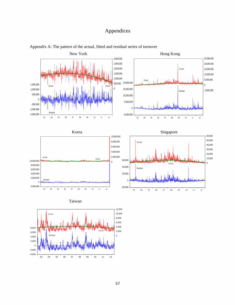
57

Appendices

Appendix A: The pattern of the actual, fitted and residual series of turnover

New York Hong Kong

Korea Singapore

Taiwan

-20,000

0

20,000

40,000

60,0000

10,000

20,000

30,000

40,000

50,000

60,000

03 04 05 06 07 08 09 10 11 12

Residual

Actual

Fitted

-1,500,000

-1,000,000

-500,000

0

500,000

1,000,000

1,500,000

0

500,000

1,000,000

1,500,000

2,000,000

2,500,000

3,000,000

03 04 05 06 07 08 09 10 11 12

Residual

Actual Fitted

-5,000,000

0

5,000,000

10,000,000

15,000,000

20,000,000

-5,000,000

0

5,000,000

10,000,000

15,000,000

20,000,000

25,000,000

03 04 05 06 07 08 09 10 11 12

Residual

Actual

Fitted

-2,000,000

0

2,000,000

4,000,000

6,000,000

8,000,000

10,000,000 0

2,000,000

4,000,000

6,000,000

8,000,000

10,000,000

03 04 05 06 07 08 09 10 11 12

Residual

ActualFitted

-4,000

-2,000

0

2,000

4,000

6,000

8,000

0

2,000

4,000

6,000

8,000

10,000

12,000

03 04 05 06 07 08 09 10 11 12

Residual

Actual

Fitted

58

Appendix B: ARIMA (1, 1, 1), residuals autocorrelation

New York Hong Kong

ACF PACF AC PAC Q-Stat Prob Autocorrelation

Partial

Correlation AC PAC Q-Stat Prob

*| | *| | 1 -0.09 -0.09 20.38 | | | | 1 -0.03 -0.03 2.1822

| | | | 2 -0.028 -0.036 22.34 | | | | 2 -0.008 -0.009 2.3331

| | | | 3 0.012 0.006 22.718 0.000 | | | | 3 -0.015 -0.016 2.9263 0.087

| | | | 4 -0.003 -0.003 22.749 0.000 | | | | 4 -0.008 -0.009 3.0675 0.216

| | | | 5 -0.043 -0.044 27.469 0.000 | | | | 5 -0.011 -0.011 3.3469 0.341

| | | | 6 -0.008 -0.016 27.628 0.000 | | | | 6 -0.015 -0.016 3.9049 0.419

| | | | 7 -0.015 -0.02 28.2 0.000 | | | | 7 0.024 0.023 5.385 0.371

| | | | 8 0.016 0.012 28.815 0.000 | | | | 8 0.02 0.02 6.3322 0.387

| | | | 9 -0.006 -0.005 28.903 0.000 | | | | 9 -0.022 -0.021 7.502 0.379

| | | | 10 0.04 0.039 32.96 0.000 | | | | 10 -0.029 -0.029 9.5474 0.298

South Korea Singapore

ACF PACF AC PAC Q-Stat Prob ACF PACF AC PAC Q-Stat Prob

| | | | 1 0.024 0.024 1.4274 | | | | 1 0 0 0.0003

| | | | 2 -0.031 -0.031 3.7376 | | | | 2 -0.028 -0.028 1.5308

| | | | 3 0.017 0.018 4.4336 0.035 | | | | 3 0.035 0.035 3.9402 0.047

| | | | 4 -0.032 -0.033 6.8938 0.032 | | | | 4 -0.029 -0.03 5.6731 0.059

| | | | 5 -0.018 -0.015 7.6559 0.054 | | | | 5 0.018 0.02 6.343 0.096

| | | | 6 -0.007 -0.009 7.7806 0.1 | | | | 6 0.068 0.065 15.572 0.004

| | | | 7 0.027 0.028 9.5738 0.088 | | | | 7 0.018 0.021 16.256 0.006

| | | | 8 -0.004 -0.006 9.6151 0.142 | | | | 8 -0.017 -0.015 16.811 0.01

| | | | 9 0.002 0.003 9.6237 0.211 | | | | 9 -0.013 -0.016 17.162 0.016

| | | | 10 0.011 0.009 9.9267 0.27 | | | | 10 0.02 0.021 17.943 0.022

59

Appendix B: Continued

Taiwan

ACF PACF AC PAC Q-Stat Prob

| | | | 1 0.058 0.058 8.2192

| | | | 2 -0.006 -0.009 8.303

| | | | 3 0.014 0.015 8.7789 0.003

| | | | 4 -0.021 -0.022 9.8348 0.007

| | | | 5 -0.023 -0.021 11.196 0.011

| | | | 6 -0.055 -0.053 18.693 0.001

| | | | 7 0.02 0.026 19.647 0.001

| | | | 8 0.03 0.027 21.94 0.001

| | | | 9 -0.011 -0.013 22.216 0.002

| | | | 10 0.001 0 22.22 0.005

Appendix C: The markets turnover correlogram

New York

Hong Kong

AC PAC AC PAC

Q-

Stat Prob AC PAC AC PAC

Q-

Stat Prob

|***** | |***** | 1 0.715 0.715 1287 0.000 |***** | |***** | 1 0.677 0.677 1135 0.000

|***** | |** | 2 0.666 0.318 2406.9 0.000 |***** | |** | 2 0.626 0.31 2107.1 0.000

|**** | |* | 3 0.617 0.147 3366.5 0.000 |**** | |* | 3 0.596 0.191 2988.3 0.000

|**** | |* | 4 0.598 0.133 4269.4 0.000 |**** | |* | 4 0.592 0.171 3856 0.000

|**** | |* | 5 0.603 0.154 5186.7 0.000 |**** | |* | 5 0.57 0.103 4661.8 0.000

|**** | | | 6 0.571 0.048 6009.1 0.000 |**** | |* | 6 0.559 0.091 5438.7 0.000

|**** | | | 7 0.54 0.011 6744.6 0.000 |**** | |* | 7 0.555 0.088 6203.7 0.000

|**** | | | 8 0.53 0.052 7453.6 0.000 |**** | | | 8 0.53 0.029 6900.5 0.000

|**** | |* | 9 0.532 0.078 8169.1 0.000 |**** | |* | 9 0.542 0.089 7629.4 0.000

|**** | |* | 10 0.545 0.095 8920.4 0.000 |**** | |* | 10 0.543 0.078 8362.4 0.000

60

Appendix C: Continued

Korea

Singapore

AC PAC AC PAC Q-Stat Prob AC PAC AC PAC

Q-Stat Prob

|** | |** | 1 0.274 0.274 185.34 0.000 |***** | |***** | 1 0.657 0.657 1085.6 0.000

|** | |* | 2 0.257 0.197 348.74 0.000 |**** | |** | 2 0.557 0.222 1868.2 0.000

|** | |* | 3 0.251 0.158 504.78 0.000 |**** | |* | 3 0.514 0.155 2534.1 0.000

|** | |* | 4 0.231 0.113 636.6 0.000 |**** | |* | 4 0.492 0.124 3143 0.000

|** | |* | 5 0.224 0.096 760.95 0.000 |*** | |* | 5 0.473 0.095 3707.9 0.000

|** | |* | 6 0.22 0.085 881.17 0.000 |*** | |* | 6 0.473 0.106 4271.6 0.000

|** | |* | 7 0.215 0.074 996.03 0.000 |*** | | | 7 0.428 0.006 4733.6 0.000

|* | | | 8 0.206 0.06 1101.6 0.000 |*** | |* | 8 0.43 0.076 5200.1 0.000

|** | |* | 9 0.231 0.089 1234.5 0.000 |*** | | | 9 0.427 0.059 5660 0.000

|* | | | 10 0.189 0.028 1323.5 0.000 |*** | | | 10 0.43 0.067 6126.3 0.000

AC PAC AC PAC Q-Stat Prob

|******| |******| 1 0.835 0.835 1730.2 0.000

|******| |** | 2 0.777 0.262 3227.6 0.000

|***** | |* | 3 0.734 0.131 4566.6 0.000

|***** | |* | 4 0.702 0.087 5789.7 0.000

|***** | |* | 5 0.683 0.094 6948.5 0.000

|***** | | | 6 0.655 0.03 8015 0.000

|**** | | | 7 0.623 -0 8979.4 0.000

|**** | | | 8 0.603 0.034 9883.5 0.000

|**** | |* | 9 0.603 0.098 10789 0.000

|**** | | | 10 0.592 0.036 11663 0.000

Taiwan

61

Appendix D: ARIMA (1, 1, 1), squared residual correlogram

New York Hong Kong South Korea Singapore Taiwan

lag ACF PACF ACF PACF ACF PACF ACF PACF ACF PACF

1 |* | |* | |*** | |*** | |* | |* | | | | | |* | |* |

2 |*** | |*** | |*** | |** | |** | |** | | | | | |* | |* |

3 |* | |* | |** | |* | |* | |* | | | | | |* | |* |

4 |** | |* | |** | |* | |** | |* | | | | | |* | | |

5 |** | |** | |** | | | |** | |* | | | | | |* | |* |

6 |** | |* | |* | | | |** | |* | |* | |* | |* | | |

7 |** | |* | |* | | | |* | | | |* | | | |* | | |

8 |** | | | |** | |* | |* | | | | | | | |* | | |

9 |** | | | |* | | | |* | | | |* | |* | |* | | |

10 |** | |* | |** | |* | |** | |* | | | | | |* | | |

11 |** | |* | |** | | | |* | | | |* | |* | |* | |* |

12 |** | | | |** | | | |* | | | | | | | |* | | |

13 |* | *| | |** | | | |* | | | | | | | |* | | |

14 |* | *| | |** | | | |* | | | | | | | |* | | |

15 |* | | | |* | | | |* | | | |* | | | |* | | |

16 |** | | | |* | | | |* | | | | | | | |* | | |

17 |** | | | |* | | | |* | | | | | | | | | | |

18 |** | | | |* | | | |* | | | |* | | | |* | | |

19 |* | | | |* | | | |* | | | | | | | | | | |

20 |** | | | |* | | | |* | | | | | | | | | | |

21 |** | | | |* | | | |* | | | |* | | | |* | | |

22 |* | | | |* | | | |* | | | | | | | |* | | |

23 |** | | | |* | |* | |* | |* | | | | | |* | | |

24 |* | | | |* | | | |* | | | | | | | |* | | |

62

Appendix E: Impulse response of volume on return and vice versa

-0.4

0.0

0.4

0.8

1.2

1.6

1 2 3 4 5 6 7 8 9 10

Response of Return to Return

-0.4

0.0

0.4

0.8

1.2

1.6

1 2 3 4 5 6 7 8 9 10

Response of Return to Volume

-0.25

0.00

0.25

0.50

0.75

1.00

1 2 3 4 5 6 7 8 9 10

Response of Volume to Return

-0.25

0.00

0.25

0.50

0.75

1.00

1 2 3 4 5 6 7 8 9 10

Response of Volume to Volume

New York

Response to Cholesky One S.D. Innovations ± 2 S.E.

-0.4

0.0

0.4

0.8

1.2

1.6

2.0

1 2 3 4 5 6 7 8 9 10

Response of Return to Return

-0.4

0.0

0.4

0.8

1.2

1.6

2.0

1 2 3 4 5 6 7 8 9 10

Response of Return to Volume

-0.2

0.0

0.2

0.4

0.6

0.8

1.0

1 2 3 4 5 6 7 8 9 10

Response of Volume to Return

-0.2

0.0

0.2

0.4

0.6

0.8

1.0

1 2 3 4 5 6 7 8 9 10

Response of Volume to Volume

Hong KongResponse to Cholesky One S.D. Innovations ± 2 S.E.

63

Appendix E: Continued

-0.4

0.0

0.4

0.8

1.2

1.6

1 2 3 4 5 6 7 8 9 10

Response of return to return

-0.4

0.0

0.4

0.8

1.2

1.6

1 2 3 4 5 6 7 8 9 10

Response of return to volume

-0.2

0.0

0.2

0.4

0.6

0.8

1.0

1 2 3 4 5 6 7 8 9 10

Response of volume to return

-0.2

0.0

0.2

0.4

0.6

0.8

1.0

1 2 3 4 5 6 7 8 9 10

Response of volume to volume

South KoreaResponse to Cholesky One S.D. Innovations ± 2 S.E.

0.0

0.4

0.8

1.2

1 2 3 4 5 6 7 8 9 10

Response of return to return

0.0

0.4

0.8

1.2

1 2 3 4 5 6 7 8 9 10

Response of return to volume

-0.25

0.00

0.25

0.50

0.75

1.00

1 2 3 4 5 6 7 8 9 10

Response of volume to return

-0.25

0.00

0.25

0.50

0.75

1.00

1 2 3 4 5 6 7 8 9 10

Response of volume to volume

Singapore

Response to Cholesky One S.D. Innovations ± 2 S.E.

64

Appendix E: Continued

Appendix F: Impulse Response of Volatility on Volume and vice versa

-0.4

0.0

0.4

0.8

1.2

1.6

1 2 3 4 5 6 7 8 9 10

Response of return to return

-0.4

0.0

0.4

0.8

1.2

1.6

1 2 3 4 5 6 7 8 9 10

Response of return to volume

.0

.1

.2

.3

.4

.5

.6

1 2 3 4 5 6 7 8 9 10

Response of volume to return

.0

.1

.2

.3

.4

.5

.6

1 2 3 4 5 6 7 8 9 10

Response of volume to volume

TaiwanResponse to Cholesky One S.D. Innovations ± 2 S.E.

-2

0

2

4

6

8

1 2 3 4 5 6 7 8 9 10

Response of volatility to volatility

-2

0

2

4

6

8

1 2 3 4 5 6 7 8 9 10

Response of volatility to volume

0.0

0.2

0.4

0.6

0.8

1.0

1 2 3 4 5 6 7 8 9 10

Response of volume to volatility

0.0

0.2

0.4

0.6

0.8

1.0

1 2 3 4 5 6 7 8 9 10

Response of volume to volume

New YorkResponse to Cholesky One S.D. Innovations ± 2 S.E.

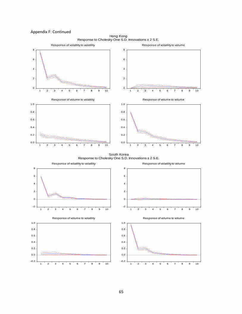
65

Appendix F: Continued

0

2

4

6

8

1 2 3 4 5 6 7 8 9 10

Response of volatility to volatility

0

2

4

6

8

1 2 3 4 5 6 7 8 9 10

Response of volatility to volume

0.0

0.2

0.4

0.6

0.8

1.0

1 2 3 4 5 6 7 8 9 10

Response of volume to volatility

0.0

0.2

0.4

0.6

0.8

1.0

1 2 3 4 5 6 7 8 9 10

Response of volume to volume

Hong KongResponse to Cholesky One S.D. Innovations ± 2 S.E.

-2

0

2

4

6

8

1 2 3 4 5 6 7 8 9 10

Response of volatility to volatility

-2

0

2

4

6

8

1 2 3 4 5 6 7 8 9 10

Response of volatility to volume

-0.2

0.0

0.2

0.4

0.6

0.8

1.0

1 2 3 4 5 6 7 8 9 10

Response of volume to volatility

-0.2

0.0

0.2

0.4

0.6

0.8

1.0

1 2 3 4 5 6 7 8 9 10

Response of volume to volume

South KoreaResponse to Cholesky One S.D. Innovations ± 2 S.E.

66

Appendix F: Continued

-1

0

1

2

3

4

1 2 3 4 5 6 7 8 9 10

Response of volatility to volatility

-1

0

1

2

3

4

1 2 3 4 5 6 7 8 9 10

Response of volatility to volume

0.0

0.2

0.4

0.6

0.8

1.0

1 2 3 4 5 6 7 8 9 10

Response of volume to volatility

0.0

0.2

0.4

0.6

0.8

1.0

1 2 3 4 5 6 7 8 9 10

Response of volume to volume

SingaporeResponse to Cholesky One S.D. Innovations ± 2 S.E.

-1

0

1

2

3

4

5

1 2 3 4 5 6 7 8 9 10

Response of volatility to volatility

-1

0

1

2

3

4

5

1 2 3 4 5 6 7 8 9 10

Response of volatility to volume

.0

.1

.2

.3

.4

.5

.6

1 2 3 4 5 6 7 8 9 10

Response of volume to volatility

.0

.1

.2

.3

.4

.5

.6

1 2 3 4 5 6 7 8 9 10

Response of volume to volume

TaiwanResponse to Cholesky One S.D. Innovations ± 2 S.E.

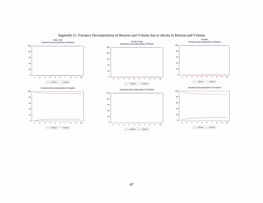
67

Appendix G: Variance Decomposition of Returns and Volume due to shocks in Returns and Volume

0

20

40

60

80

100

1 2 3 4 5 6 7 8 9 10

Return Volume

New York

Variance Decomposition of Return

0

20

40

60

80

100

1 2 3 4 5 6 7 8 9 10

Return Volume

Variance Decomposition of Volume

0

20

40

60

80

100

1 2 3 4 5 6 7 8 9 10

Return Volume

Hong Kong

Variance Decomposition of Return

0

20

40

60

80

100

1 2 3 4 5 6 7 8 9 10

Return Volume

Variance Decomposition of Volume

0

20

40

60

80

100

1 2 3 4 5 6 7 8 9 10

Return Volume

Taiwan

Variance Decomposition of Return

0

20

40

60

80

100

1 2 3 4 5 6 7 8 9 10

Return Volume

Variance Decomposition of Volume

68

Appendix G: Continued

0

20

40

60

80

100

1 2 3 4 5 6 7 8 9 10

Return Volume

Korea

Variance Decomposition of Return

0

20

40

60

80

100

1 2 3 4 5 6 7 8 9 10

Return Volume

Variance Decomposition of Volume

0

20

40

60

80

100

1 2 3 4 5 6 7 8 9 10

Return Volume

Singapore

Variance Decomposition of Return

0

20

40

60

80

100

1 2 3 4 5 6 7 8 9 10

Return Volume

Variance Decomposition of Volume