Traffic Measurement Traffic Measurement for IP Operationsfor IP Operations

Jennifer RexfordInternet and Networking Systems

AT&T Labs - Research; Florham Park, NJhttp://www.research.att.com/~jrex

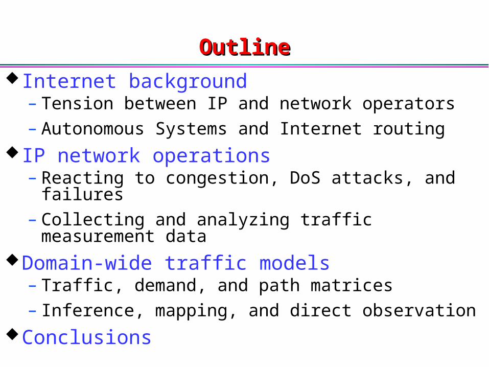
OutlineOutline

Internet background– Tension between IP and network operators

– Autonomous Systems and Internet routingIP network operations

– Reacting to congestion, DoS attacks, and failures

– Collecting and analyzing traffic measurement dataDomain-wide traffic models

– Traffic, demand, and path matrices

– Inference, mapping, and direct observationConclusions

Characteristics of the InternetCharacteristics of the Internet

The Internet is– Decentralized (loose confederation of peers)

– Self-configuring (no global registry of topology)

– Stateless (limited information in the routers)

– Connectionless (no fixed connection between hosts)

These attributes contribute– To the success of Internet

– To the rapid growth of the Internet

– … and the difficulty of controlling the Internet!

ISPsender receiver

Operator Philosophy: Tension With IPOperator Philosophy: Tension With IP

Accountability of network resources– But, routers don’t maintain state about transfers

– But, measurement isn’t part of the infrastructure

Reliability/predictability of services– But, IP doesn’t provide performance guarantees

– But, equipment is not especially reliable (no “five-9s”)

Fine-grain control over the network– But, routers don’t do fine-grain resource allocation

– But, network automatically re-routes after failures

End-to-end control over communication– But, end hosts and applications adapt to congestion

– But, traffic may traverse multiple domains of control

And Now Some Good News…And Now Some Good News…

This makes for great research problems!

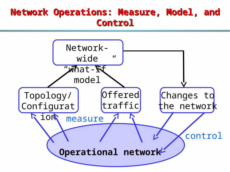
Network Operations: Measure, Model, and ControlNetwork Operations: Measure, Model, and Control

Topology/Configuratio

n

Offeredtraffic

Changes tothe network

Operational network

Network-wide“what-if”

model

measure

control

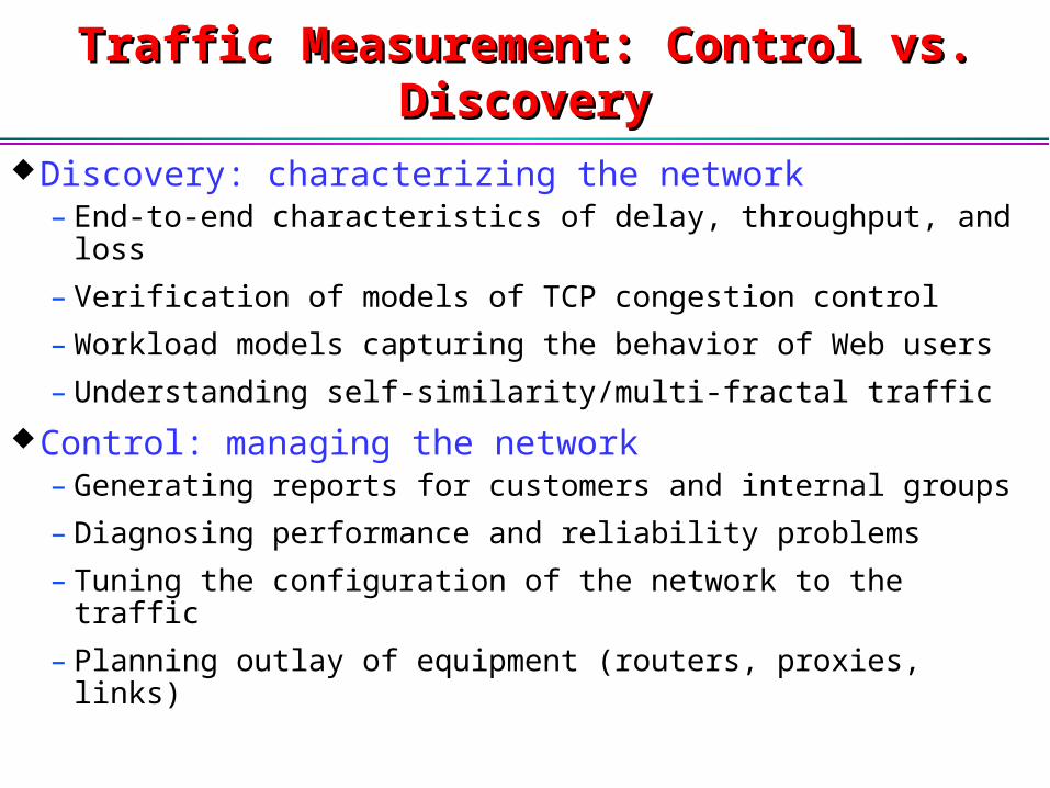
Traffic Measurement: Control vs. DiscoveryTraffic Measurement: Control vs. Discovery

Discovery: characterizing the network– End-to-end characteristics of delay, throughput, and loss

– Verification of models of TCP congestion control

– Workload models capturing the behavior of Web users

– Understanding self-similarity/multi-fractal traffic

Control: managing the network– Generating reports for customers and internal groups

– Diagnosing performance and reliability problems

– Tuning the configuration of the network to the traffic

– Planning outlay of equipment (routers, proxies, links)

Autonomous Systems (ASes)Autonomous Systems (ASes)

Internet divided into ASes– Distinct regions of administrative control (~14,000)

– Routers and links managed by a single institution

Internet hierarchy– Large, tier-1 provider with a nationwide backbone

– Medium-sized regional provider w/ smaller backbone

– Smaller network run by single company or university

Interaction between ASes– Internal topology is not shared between ASes

– … but, neighbor ASes interact to coordinate routing

AS-Level Graph of the InternetAS-Level Graph of the Internet

1

2

3

4

5

67

ClientWeb server

AS path: 6, 5, 4, 3, 2, 1

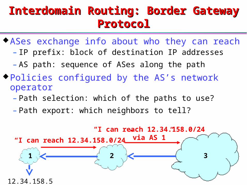
Interdomain Routing: Border Gateway ProtocolInterdomain Routing: Border Gateway Protocol

ASes exchange info about who they can reach– IP prefix: block of destination IP addresses

– AS path: sequence of ASes along the path

Policies configured by the AS’s network operator– Path selection: which of the paths to use?

– Path export: which neighbors to tell?

1 2 3

12.34.158.5

“I can reach 12.34.158.0/24”

“I can reach 12.34.158.0/24 via AS 1”

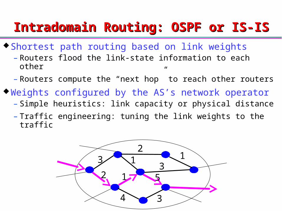
Intradomain Routing: OSPF or IS-ISIntradomain Routing: OSPF or IS-IS

Shortest path routing based on link weights– Routers flood the link-state information to each other

– Routers compute the “next hop” to reach other routers

Weights configured by the AS’s network operator– Simple heuristics: link capacity or physical distance

– Traffic engineering: tuning the link weights to the traffic

32

2

1

13

1

4

5

3

““Operations” Research: Detect, Diagnose, and FixOperations” Research: Detect, Diagnose, and Fix

Detect: note the symptoms of a problem– Periodic polling of link load statistics

– Active probes measuring performance

– Customer complaining (via the phone network?)

Diagnose: identify the illness– Change in user behavior?

– Router/link failure or policy change?

– Denial of service attack?

Fix: select and dispense the medicine– Routing protocol reconfiguration

– Installation of packet filters

Network measurement plays a key role in each step!

Time Scales for Network OperationsTime Scales for Network Operations

Minutes to hours– Denial-of-service attacks

– Router and link failures

– Serious congestionHours to weeks

– Time-of-day or day-of-week engineering

– Outlay of new routers and links

– Addition/deletion of customers or peersWeeks to years

– Planning of new capacity and topology changes

– Evaluation of network designs and routing protocols

Traffic Measurement: SNMP DataTraffic Measurement: SNMP Data

Simple Network Management Protocol (SNMP)– Router CPU utilization, link utilization, link loss, …

– Collected from every router/link every few minutes

Applications– Detecting overloaded links and sudden traffic shifts

– Inferring the domain-wide traffic matrix

Advantage– Open standard, available for every router and link

Disadvantage– Coarse granularity, both spatially and temporally

Traffic Measurement: Packet-Level TracesTraffic Measurement: Packet-Level TracesPacket monitoring

– IP, TCP/UDP, and application-level headers– Collected by tapping individual links in the network

Applications– Fine-grain timing of the packets on the link– Fine-grain view of packet header fields

Advantages– Most detailed view possible at the IP level

Disadvantages– Expensive to have in more than a few locations– Challenging to collect on very high-speed links– Extremely high volume of measurement data

Extracting Data from IP PacketsExtracting Data from IP Packets

IPTCP

IPTCP

IPTCP

Application message (e.g., HTTP response)

Many layers of information– IP: source/dest IP addresses, protocol (TCP/UDP), …

– TCP/UDP: src/dest port numbers, seq/ack, flags, …

– Application: URL, user keystrokes, BGP updates,…

flow 1 flow 2 flow 3 flow 4

Aggregating Packets into FlowsAggregating Packets into Flows

Set of packets that “belong together”– Source/destination IP addresses and port numbers

– Same protocol, ToS bits, …

– Same input/output interfaces at a router (if known)

Packets that are “close” together in time– Maximum inter-packet spacing (e.g., 15 sec, 30 sec)

– Example: flows 2 and 4 are different flows due to time

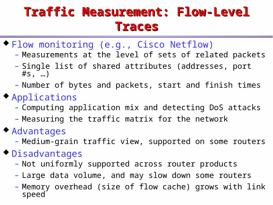
Traffic Measurement: Flow-Level TracesTraffic Measurement: Flow-Level Traces Flow monitoring (e.g., Cisco Netflow)

– Measurements at the level of sets of related packets

– Single list of shared attributes (addresses, port #s, …)

– Number of bytes and packets, start and finish times Applications

– Computing application mix and detecting DoS attacks

– Measuring the traffic matrix for the network Advantages

– Medium-grain traffic view, supported on some routers Disadvantages

– Not uniformly supported across router products

– Large data volume, and may slow down some routers

– Memory overhead (size of flow cache) grows with link speed

Reducing Packet/Flow Measurement OverheadReducing Packet/Flow Measurement Overhead

Filtering: select a subset of the traffic– E.g., destination prefix for a customer

– E.g., port number for an application (e.g., 80 for Web)

Aggregation: grouping related traffic– E.g., packets/flows with same next-hop AS

– E.g., packets/flows destined to a particular service

Sampling: subselecting the traffic– Random, deterministic, or hash-based sampling

– 1-out-of-n or stratified based on packet/flow size

Combining filtering, aggregation, and sampling

Comparison of TechniquesComparison of Techniques

SamplingSamplingFilteringFiltering AggregationAggregation

Generality

LocalProcessing

Local memory

Compression

Precision exact exact approximate

constraineda-priori

constraineda-priori

general

filter criterionfor every object

table updatefor every object

only samplingdecision

none one bin pervalue of interest

none

dependson data

dependson data controlled

Traffic Representations for Network OperatorsTraffic Representations for Network Operators

Network-wide views– Not directly supported by IP (stateless, decentralized)

– Combining traffic, topology, and state information

Challenges– Assumptions about the properties of the traffic

– Assumptions about the topology and routing

– Assumptions about the support for measurement

Models: traffic, demand, and path matrices– Populating the models from measurement data

– Recent proposals for new types of measurements

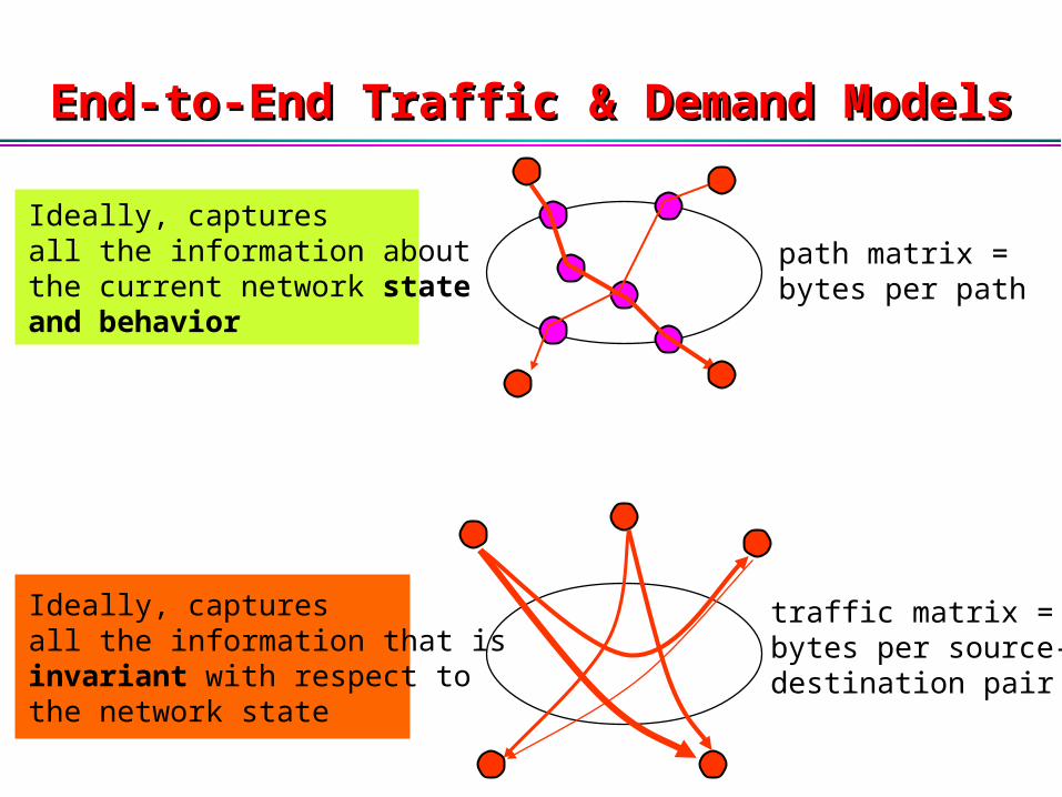
End-to-End Traffic & Demand ModelsEnd-to-End Traffic & Demand Models

path matrix = bytes per path

traffic matrix =bytes per source-destination pair

Ideally, capturesall the information about the current network state and behavior

Ideally, capturesall the information that isinvariant with respect to the network state

Domain-Wide Network Traffic ModelsDomain-Wide Network Traffic Models

current state &traffic flow

fine grained:path matrix = bytes per path

intradomain focus:traffic matrix =bytes per ingress-egress

interdomain focus:demand matrix =bytes per ingress andset of possible egresses

predictedcontrol action:impact of intra-domain routing

predictedcontrol action:impact of inter-domain routing

Path Matrix: Operational UsesPath Matrix: Operational Uses

Congested link– Problem: easy to detect, hard to diagnose

– Which traffic is responsible? Which traffic affected?

Customer complaint– Problem: customer has limited visibility to diagnose

– How is the traffic of a given customer routed?

– Where does the traffic experience loss and delay?

Denial-of-service attack– Problem: spoofed source address, distributed attack

– Where is the attack coming from? Who is affected?

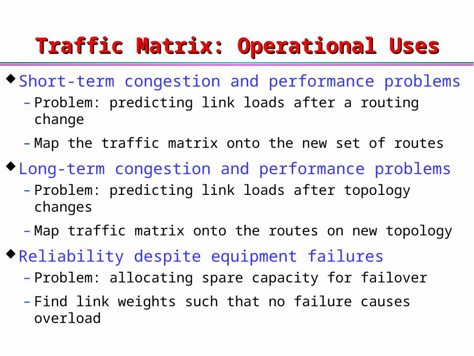
Traffic Matrix: Operational UsesTraffic Matrix: Operational Uses

Short-term congestion and performance problems– Problem: predicting link loads after a routing change

– Map the traffic matrix onto the new set of routes

Long-term congestion and performance problems– Problem: predicting link loads after topology changes

– Map traffic matrix onto the routes on new topology

Reliability despite equipment failures– Problem: allocating spare capacity for failover

– Find link weights such that no failure causes overload

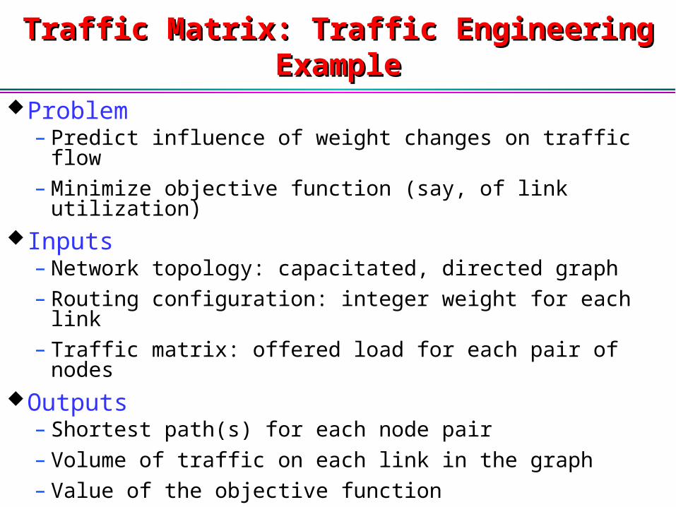
Traffic Matrix: Traffic Engineering ExampleTraffic Matrix: Traffic Engineering Example

Problem – Predict influence of weight changes on traffic flow

– Minimize objective function (say, of link utilization)Inputs

– Network topology: capacitated, directed graph

– Routing configuration: integer weight for each link

– Traffic matrix: offered load for each pair of nodesOutputs

– Shortest path(s) for each node pair

– Volume of traffic on each link in the graph

– Value of the objective function

Demand Matrix: Motivating ExampleDemand Matrix: Motivating Example

Big Internet

Web Site User Site

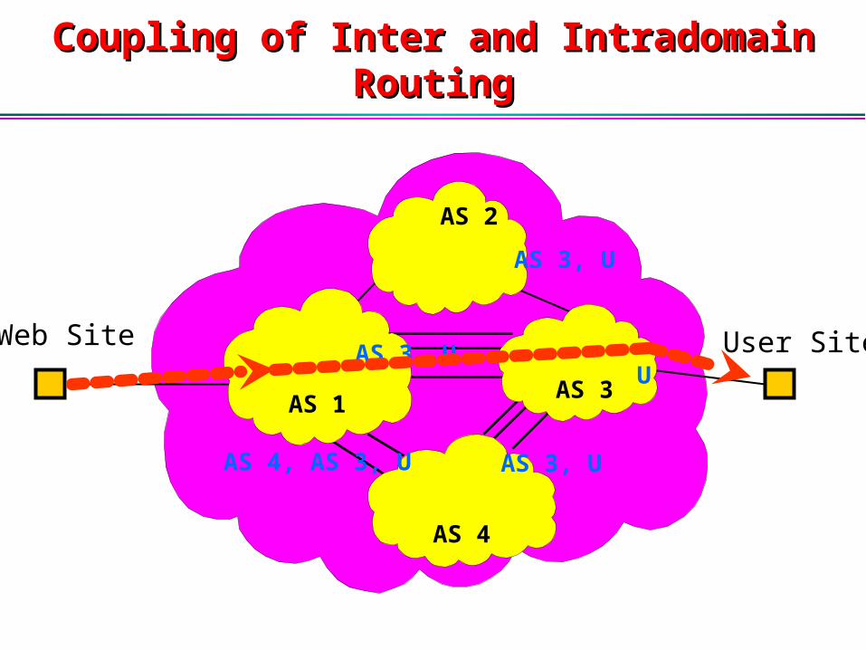
Coupling of Inter and Intradomain RoutingCoupling of Inter and Intradomain Routing

Web Site User Site

AS 1AS 3

AS 4

U

AS 3, U

AS 3, U

AS 3, U

AS 4, AS 3, U

AS 2

Intradomain Routing: Hot PotatoIntradomain Routing: Hot Potato

Zoom in on AS1

200

11010

110

300

25

75

110

300

IN

OUT 2

110

Hot-potato routing: change in internal routing (link weights)

configuration changes flow exit point!

50

OUT 3

OUT 1

Demand Model: Operational UsesDemand Model: Operational Uses

Coupling problem with traffic matrix approach

Demands: # bytes for each (in, {out_1,...,out_m})– ingress link (in)

– set of possible egress links ({out_1,...,out_m})

Traffic matrix

Traffic Engineering

Improved Routing

Traffic matrix

Traffic Engineering

Improved Routing

Demand matrix

Traffic Engineering

Improved Routing

Populating the Domain-Wide ModelsPopulating the Domain-Wide Models

Inference: assumptions about traffic and routing– Traffic data: byte counts per link (over time)

– Routing data: path(s) between each pair of nodes

Mapping: assumptions about routing– Traffic data: packet/flow statistics at network edge

– Routing data: egress point(s) per destination prefix

Direct observation: no assumptions– Traffic data: packet samples at every link

– Routing data: none

4Mbps 4Mbps

3Mbps5Mbps

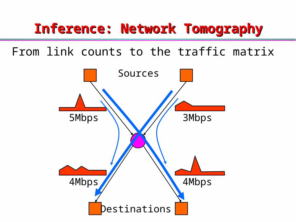
Inference: Network TomographyInference: Network Tomography

Sources

Destinations

From link counts to the traffic matrix

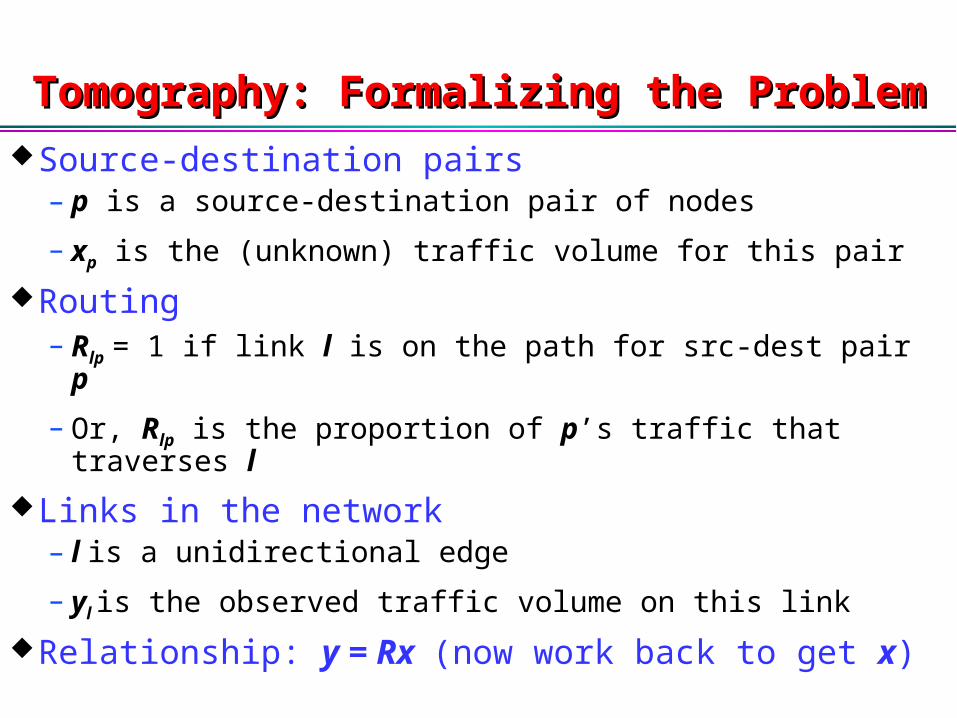
Tomography: Formalizing the ProblemTomography: Formalizing the Problem

Source-destination pairs – p is a source-destination pair of nodes

– xp is the (unknown) traffic volume for this pair

Routing– Rlp = 1 if link l is on the path for src-dest pair p

– Or, Rlp is the proportion of p’s traffic that traverses l

Links in the network– l is a unidirectional edge

– yl is the observed traffic volume on this link

Relationship: y = Rx (now work back to get x)

Tomography: Single Observation is InsufficientTomography: Single Observation is Insufficient

Linear system is underdetermined– Number of nodes n

– Number of links e is around O(n)

– Number of src-dest pairs c is O(n2)

– Dimension of solution sub-space at least c - e

Multiple observations are needed– k independent observations (over time)

– Stochastic model with src-dest counts Poisson & i.i.d

– Maximum likelihood estimation to infer traffic matrix

– Vardi, “Network Tomography,” JASA, March 1996

Tomography: ChallengesTomography: Challenges

Limitations– Cannot handle packet loss or multicast traffic

– Statistical assumptions don’t match IP traffic

– Significant error even with large # of samples

– High computation overhead for large networks

Directions for future work– More realistic assumptions about the IP traffic

– Partial queries over subgraphs in the network

– Incorporating additional measurement data

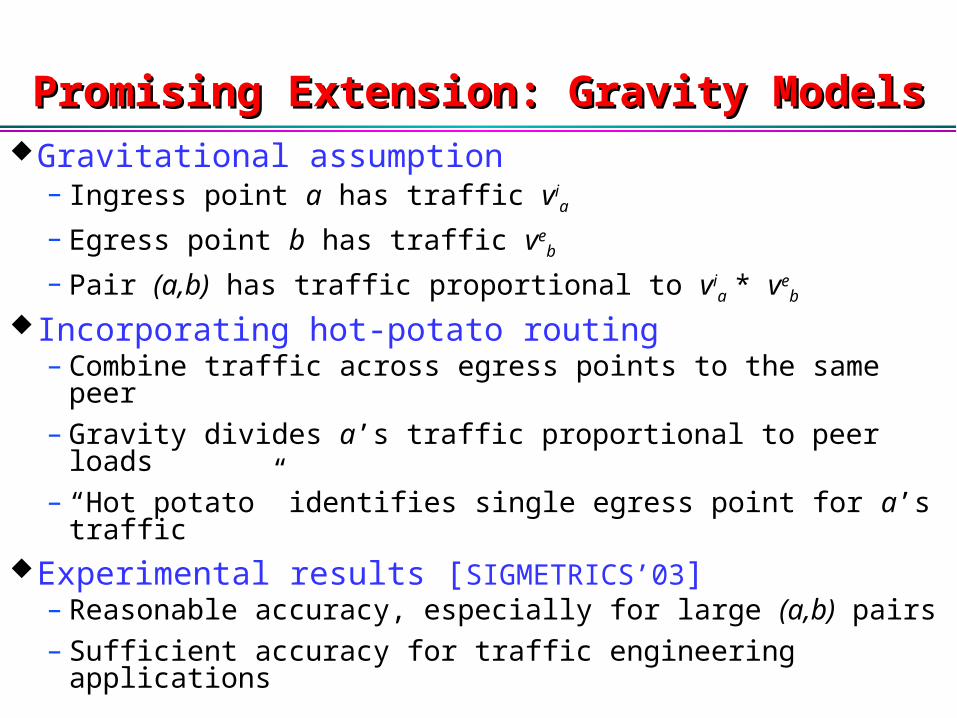
Promising Extension: Gravity ModelsPromising Extension: Gravity Models

Gravitational assumption– Ingress point a has traffic vi

a

– Egress point b has traffic veb

– Pair (a,b) has traffic proportional to via * ve

b

Incorporating hot-potato routing– Combine traffic across egress points to the same peer

– Gravity divides a’s traffic proportional to peer loads

– “Hot potato” identifies single egress point for a’s trafficExperimental results [SIGMETRICS’03]

– Reasonable accuracy, especially for large (a,b) pairs

– Sufficient accuracy for traffic engineering applications

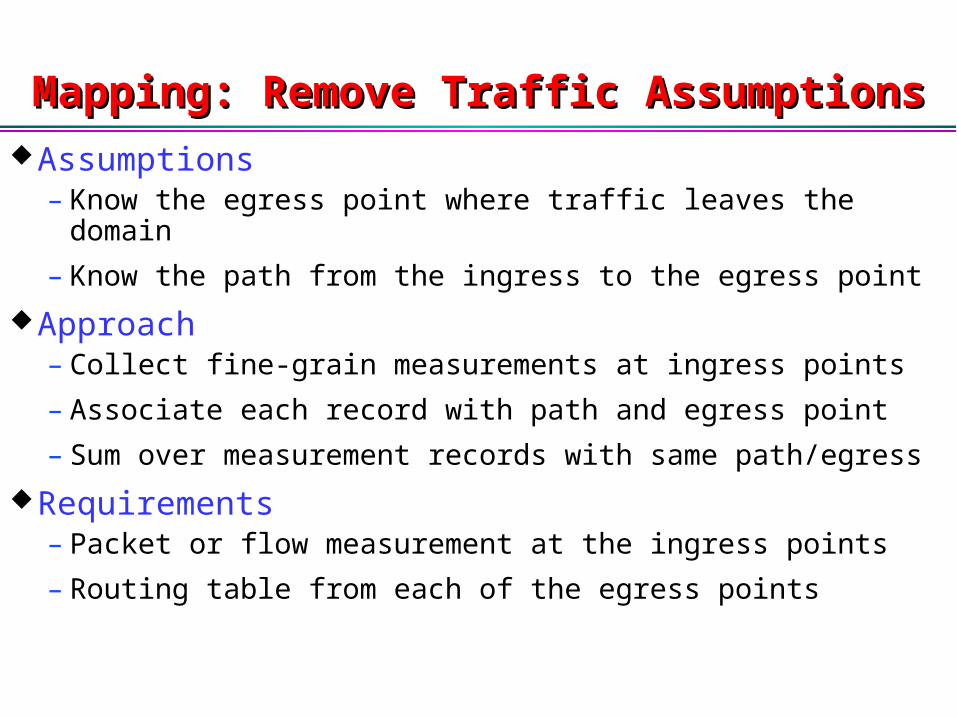
Mapping: Remove Traffic AssumptionsMapping: Remove Traffic Assumptions

Assumptions– Know the egress point where traffic leaves the domain

– Know the path from the ingress to the egress point

Approach– Collect fine-grain measurements at ingress points

– Associate each record with path and egress point

– Sum over measurement records with same path/egress

Requirements– Packet or flow measurement at the ingress points

– Routing table from each of the egress points

Traffic Mapping: Ingress MeasurementTraffic Mapping: Ingress Measurement

Traffic measurement data– Ingress point i

– Destination prefix d

– Traffic volume Vid

i dingress destination

Traffic Mapping: Egress Point(s)Traffic Mapping: Egress Point(s)

Routing data (e.g., router forwarding tables)– Destination prefix d

– Set of egress points ed

ddestination

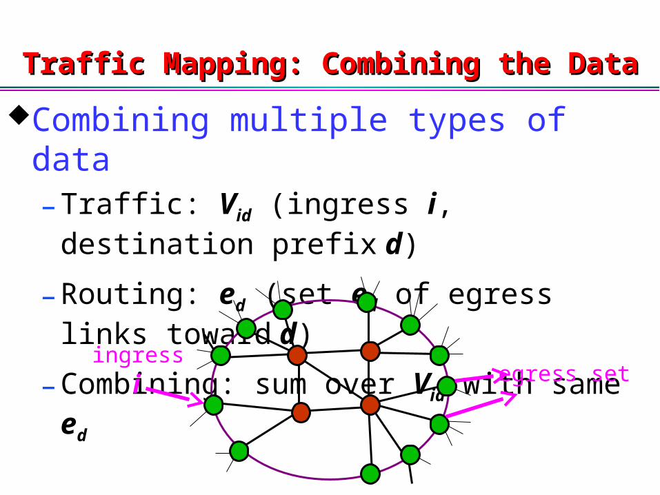
Traffic Mapping: Combining the DataTraffic Mapping: Combining the Data

Combining multiple types of data– Traffic: Vid (ingress i, destination prefix d)

– Routing: ed (set ed of egress links toward d)

– Combining: sum over Vid with same ed

iingress

egress set

Mapping: ChallengesMapping: Challenges

Limitations– Need for fine-grain data from ingress points

– Large volume of traffic measurement data

– Need for forwarding tables from egress point

– Data inconsistencies across different locations

Directions for future work– Vendor support for packet/flow measurement

– Distributed infrastructure for collecting data

– Online monitoring of topology and routing data

Direct Observation: Overcoming UncertaintyDirect Observation: Overcoming Uncertainty

Internet traffic– Fluctuation over time (burstiness, congestion control)

– Packet loss as traffic flows through the network

– Inconsistencies in timestamps across routers

IP routing protocols– Changes due to failure and reconfiguration

– Large state space (high number of links or paths)

– Vendor-specific implementation (e.g., tie-breaking)

– Multicast trees that send to (dynamic) set of receivers

Better to observe the traffic directly as it travels

Direct Observation: Straw-Man ApproachesDirect Observation: Straw-Man Approaches

Path marking– Each packet carries the path it has traversed so far

– Drawback: excessive overhead

Packet or flow measurement on every link– Combine records across all links to obtain the paths

– Drawback: excessive measurement and CPU overhead

Sample the entire path for certain packets– Sample and tag a fraction of packets at ingress point

– Sample all of the tagged packets inside the network

– Drawback: requires modification to IP (for tagging)

Direct Observation: Trajectory SamplingDirect Observation: Trajectory Sampling

Sample packets at every link without tagging– Pseudo random sampling (e.g., 1-out-of-100)

– Either sample or don’t sample at each link

– Compute a hash over the contents of the packet

Details of consistent sampling– x: subset of invariant bits in the packet

– Hash function: h(x) = x mod A

– Sample if h(x) < r, where r/A is a thinning factor

Exploit entropy in packet contents to do sampling

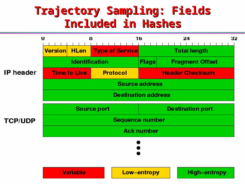
Trajectory Sampling: Fields Included in HashesTrajectory Sampling: Fields Included in Hashes

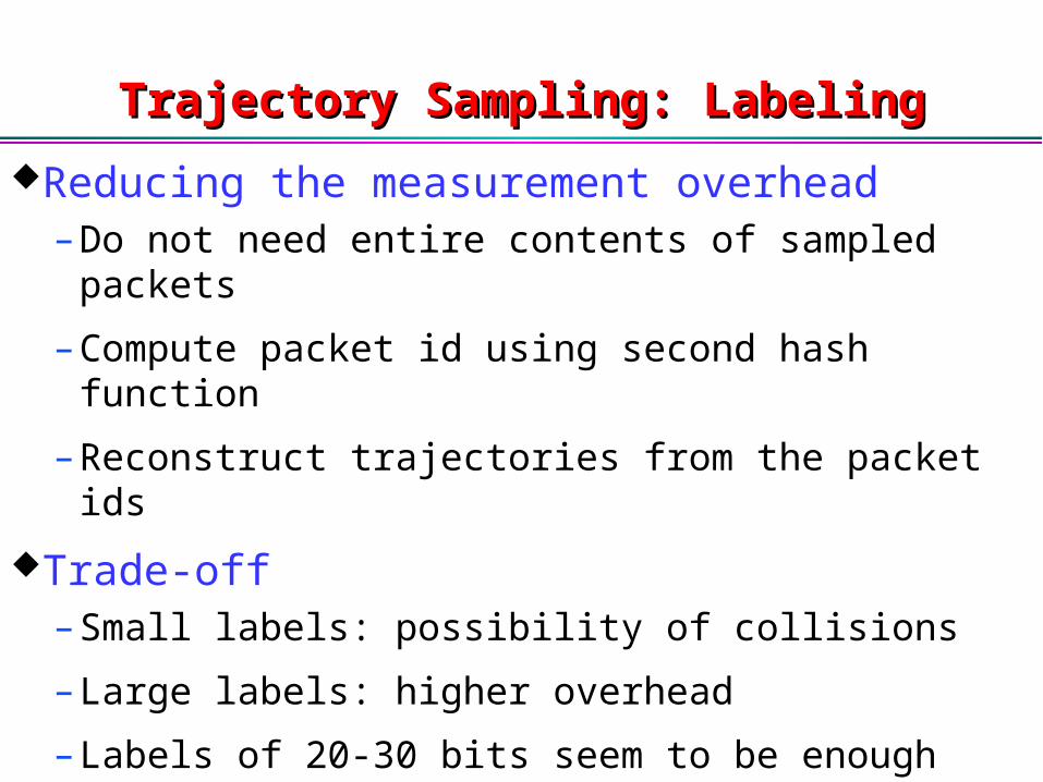
Trajectory Sampling: LabelingTrajectory Sampling: Labeling

Reducing the measurement overhead– Do not need entire contents of sampled packets

– Compute packet id using second hash function

– Reconstruct trajectories from the packet ids

Trade-off– Small labels: possibility of collisions

– Large labels: higher overhead

– Labels of 20-30 bits seem to be enough

Trajectory Sampling: Sampling and LabelingTrajectory Sampling: Sampling and Labeling

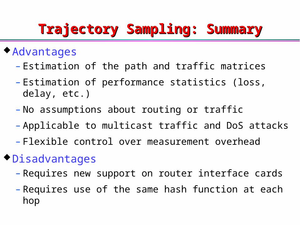
Trajectory Sampling: SummaryTrajectory Sampling: Summary

Advantages– Estimation of the path and traffic matrices

– Estimation of performance statistics (loss, delay, etc.)

– No assumptions about routing or traffic

– Applicable to multicast traffic and DoS attacks

– Flexible control over measurement overhead

Disadvantages– Requires new support on router interface cards

– Requires use of the same hash function at each hop

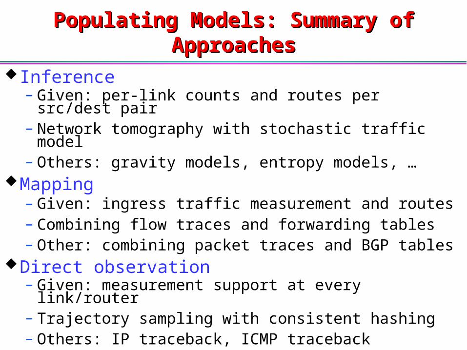
Populating Models: Summary of ApproachesPopulating Models: Summary of Approaches

Inference– Given: per-link counts and routes per src/dest pair– Network tomography with stochastic traffic model– Others: gravity models, entropy models, …

Mapping– Given: ingress traffic measurement and routes– Combining flow traces and forwarding tables– Other: combining packet traces and BGP tables

Direct observation– Given: measurement support at every link/router– Trajectory sampling with consistent hashing– Others: IP traceback, ICMP traceback

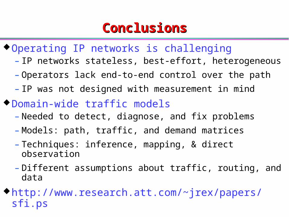
ConclusionsConclusions

Operating IP networks is challenging– IP networks stateless, best-effort, heterogeneous

– Operators lack end-to-end control over the path

– IP was not designed with measurement in mind

Domain-wide traffic models– Needed to detect, diagnose, and fix problems

– Models: path, traffic, and demand matrices

– Techniques: inference, mapping, & direct observation

– Different assumptions about traffic, routing, and data

http://www.research.att.com/~jrex/papers/sfi.ps

Interesting Research ProblemsInteresting Research ProblemsPopulating the domain-wide models

– New techniques, and combinations of techniques– Working with a mixture of different types of data

Packet/flow sampling– Traffic and performance statistics from samples– Analysis of trade-off between overhead and accuracy

Route optimization– Influence of inaccurate demand estimates on results– Optimization under traffic fluctuation and failures

Anomaly detection– Identifying fluctuations in traffic and routing data– Analyzing the data for root cause analysis