training cellular automata for image edge detection
TRANSCRIPT

ROMANIAN JOURNAL OF INFORMATIONSCIENCE AND TECHNOLOGYVolume 19, Number 4, 2016, 338–359
Training Cellular Automata for Image EdgeDetection
Anand Prakash Shukla
Department of Computer Science and Engineering,KIET Group of Institutions, Ghaziabad, INDIA
Email: [email protected]
Abstract. Cellular automata can be significantly applied in image processingtasks. In this paper, a novel method to train two dimensional cellular automata fordetection of edges in digital images has been proposed and experiments have beencarried out for the same. Training of two dimensional cellular automata meansselecting the optimum rule set from the given set of rules to perform a particulartask. In order to train the cellular automata first, the size of rule set is reduced onthe basis of symmetry. Then the sequential floating forward search method for ruleselection is used to select the best rule set for edge detection. The misclassificationerror has been used as an objective function to train the cellular automata for edgedetection. The whole experiment has been divided in two parts. First the trainingwas performed for binary images then it is performed for gray scale images. Anovel method of thresholding the image by Otsu’s algorithm and then applying thecellular automata rules for the training purpose has been proposed. It has beenobserved that the proposed method significantly decreases the training time with-out affecting the results. Results are validated and compared with some standardedge detection methods both qualitatively and quantitatively and it is found betterin terms of detecting the edges in digital images. Also the proposed method per-forms much better in corner detection as compared to the standard edge detectionmethods.
Keywords: Cellular Automata, Training of Cellular Automata,Sequential Float-ing Forward Search Algorithm, Misclassification Error, Otsu’s Algorithm, CornerDetection
1 IntroductionResearches show that any complex system is a system of several elements, operat-
ing in parallel, with neighborhood relationships that as a whole exhibit emergent globalbehavior. In other words, the complex systems are not complicated, but these are thecombinations of the many simple systems working together in parallel. Cellular au-tomata also exhibits the same. This feature of simplicity of cellular automata and theability to model complex systems has attracted the researchers’ attention from a widerange of fields.
Training Cellular Automata for Image Edge Detection 339
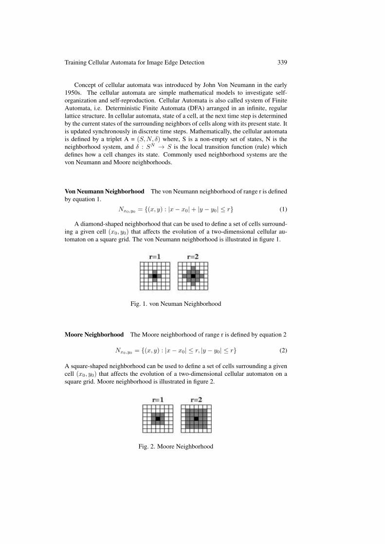
Concept of cellular automata was introduced by John Von Neumann in the early1950s. The cellular automata are simple mathematical models to investigate self-organization and self-reproduction. Cellular Automata is also called system of FiniteAutomata, i.e. Deterministic Finite Automata (DFA) arranged in an infinite, regularlattice structure. In cellular automata, state of a cell, at the next time step is determinedby the current states of the surrounding neighbors of cells along with its present state. Itis updated synchronously in discrete time steps. Mathematically, the cellular automatais defined by a triplet A = (S,N, δ) where, S is a non-empty set of states, N is theneighborhood system, and δ : SN → S is the local transition function (rule) whichdefines how a cell changes its state. Commonly used neighborhood systems are thevon Neumann and Moore neighborhoods.
Von Neumann Neighborhood The von Neumann neighborhood of range r is definedby equation 1.
Nx0,y0 = {(x, y) : |x− x0|+ |y − y0| ≤ r} (1)
A diamond-shaped neighborhood that can be used to define a set of cells surround-ing a given cell (x0, y0) that affects the evolution of a two-dimensional cellular au-tomaton on a square grid. The von Neumann neighborhood is illustrated in figure 1.
Fig. 1. von Neuman Neighborhood
Moore Neighborhood The Moore neighborhood of range r is defined by equation 2
Nx0,y0= {(x, y) : |x− x0| ≤ r, |y − y0| ≤ r} (2)
A square-shaped neighborhood can be used to define a set of cells surrounding a givencell (x0, y0) that affects the evolution of a two-dimensional cellular automaton on asquare grid. Moore neighborhood is illustrated in figure 2.
Fig. 2. Moore Neighborhood

340 A. P. Shukla
1.1 Use of Cellular Automata in Image ProcessingThe digital image is considered as a two dimensional array of M × N pixels as
shown in figure 3. Each pixel can be characterized by the triplet (i; j; k) where (i; j)represents its position in the array and k represents the associated color. The image maybe then considered as a particular configuration of a cellular automaton that occupiesthe cellular space of M × N array defined by the image. Each pixel of the imagerepresents a cell of the cellular automata and the state of the cell is defined by the valueof the pixel in image. [17]
Fig. 3. Pixel representation of Digital Image.
Cellular automata has number of advantages over traditional methods of computa-tion
• Simplicity of implementation and complexity of behavior : It is found that thecellular automata based systems can be implemented easily as each cell generallyworks on few simple rules, but a combination of these cells leads to a moresophisticated global behavior.
• CA are both inherently parallel and computationally simple.
• CA are extensible,that is, we can extend the simple rules by using some newcomputation techniques.
• One of the most important features of the CA method is that it supports n-dimensions and m-label categories where the number of labels does not increasecomputational time or complexity
• Allow efficient parallel processing of several tasks,
• Users are able to make corrections and modifications at any time during opera-tions i.e. Cellular automata is more interactive.
Some of the applications in field of image processing are noise filtering, edge de-tection, connected set morphology, and segmentation.
2 Related WorkTraining of cellular automata for an image processing task means the selection of
the optimal rule set among all the possible rules which perform best for that particular

Training Cellular Automata for Image Edge Detection 341
task. So far most of the work on cellular automata studies the effect of applying manu-ally designed transition functions(rules). The inverse of this i.e., obtaining appropriaterules to produce a desired effect is very hard. Even if only the binary images are con-sidered the combinations of all possible rules are very large. Somol et al. [27] haveshown that in some situations efficient feature selection can be performed using branchand bound algorithms and it is also tractable. However, Cover et al. [4] have shown thatin general, without an exhaustive enumeration of all combinations an optimal selectionof rules cannot be guaranteed and this is clearly impractical. One simple alternativeis to measure the effect of each rule separately and then use the results for the directconstruction of combinations of rules. However, practically some methods are requiredfor revealing at least some of the inter rule combinations.
Some authors prefer the evolutionary solutions for training of cellular automata,for example, Mitchell et al. [12] have used genetic algorithm to find the solution ofthe density classification problem. There are some difficulties reported by the authorsthemselves as breaking of symmetries in early generations (for short-term gains) thetraining data became too easy for the cellular automata in later generations of the ge-netic algorithm. This problem was solved by Julle et al. [11] by using genetic algo-rithms with co-evolution. In this method, to perform effective training, the training setwas not fixed during evolution, rather it is gradually increased as the difficulty arises.Once the cellular automata was trained for the initial solutions for simple problem, itwould be improved and extended by evolving more challenging data. Instead of geneticalgorithms, Andre et al. [1] used a standard genetic programming framework. But thismethod was computationally very expensive. Extending the density classification taskto two-dimensional grids, J Morales et al. [10] applied standard genetic algorithm totrain the cellular automata for density classification problem to two-dimensional grids.
Very less work has been done to perform the training of cellular automata for imageprocessing. One of the practical problems of using cellular automata for training is thedetermination of the rule set. The traditional methods of specifying rules manually isa slow and tedious process because of which it is unattractive. Sahota et al. [20] usedgenetic algorithm for the tasks such as edge detection in binary images. In this work, ageneralized system is set up that attempts to discover the precise cellular automata rulesrequired to solve the edge detection problem. Genetic algorithm was used to locate therules and once the system is trained it is able to process other images. Basically, thismodel works in two distinct stages - the training phase and the execution phase. Figure4 shows this training process. In the training phase, the user must supply pairs of inputand output images. The artificial images are used for this purpose. The model attemptsto find rules for the cellular automata that will provide the desired type of processing.The input patterns are first mapped onto the rule array, after which the automaton isallowed to update for a fixed number of cycles. The cellular automata rule selectorattempts to discover rapidly the rules that will produce the desired results by usinggenetic algorithm. The root mean square (RMS) error produced by each image pair ischosen as an objective function to drive the genetic algorithm. In the execution phaseonce an optimal rule set has been found for the desired problem the system is ready.New images are given as input to the trained cellular automata and it performs the taskon the basis of the optimal rules found in training phase. The results of this work showthat genetically evolved cellular automata can successfully learn the process of edgedetection for binary noise-free images.
Slatnia and Kazar [26] have used an evolutionary process to find a rule set of cel-lular automata among a set of optimal rules for extracting edges in a binary imageby applying genetic algorithm. The genetic algorithm was initialized on the basis of

342 A. P. Shukla
Fig. 4. Model for Training Cellular Automata by Genetic Algorithm [20].
random construction of the rule packets extracted from the neighborhood model asshown in figure 5. For each cellular automata rule packets(similar rule according toits neighborhood) are searched in the image then the found packet modifies the centralpixel according to the defined transition. Thereafter, distance between the result of theedges detected by this method and the ideal edges are calculated along with the error ofmiss-classed pixels. Again this method generates a new population by applying selec-tion, crossover and mutation by using the edge detection described above. This processiterates until there is no further improvement in the objective function or for a fixedmaximum number of iterations.
Fig. 5. Construction of Neighborhood Model [26].
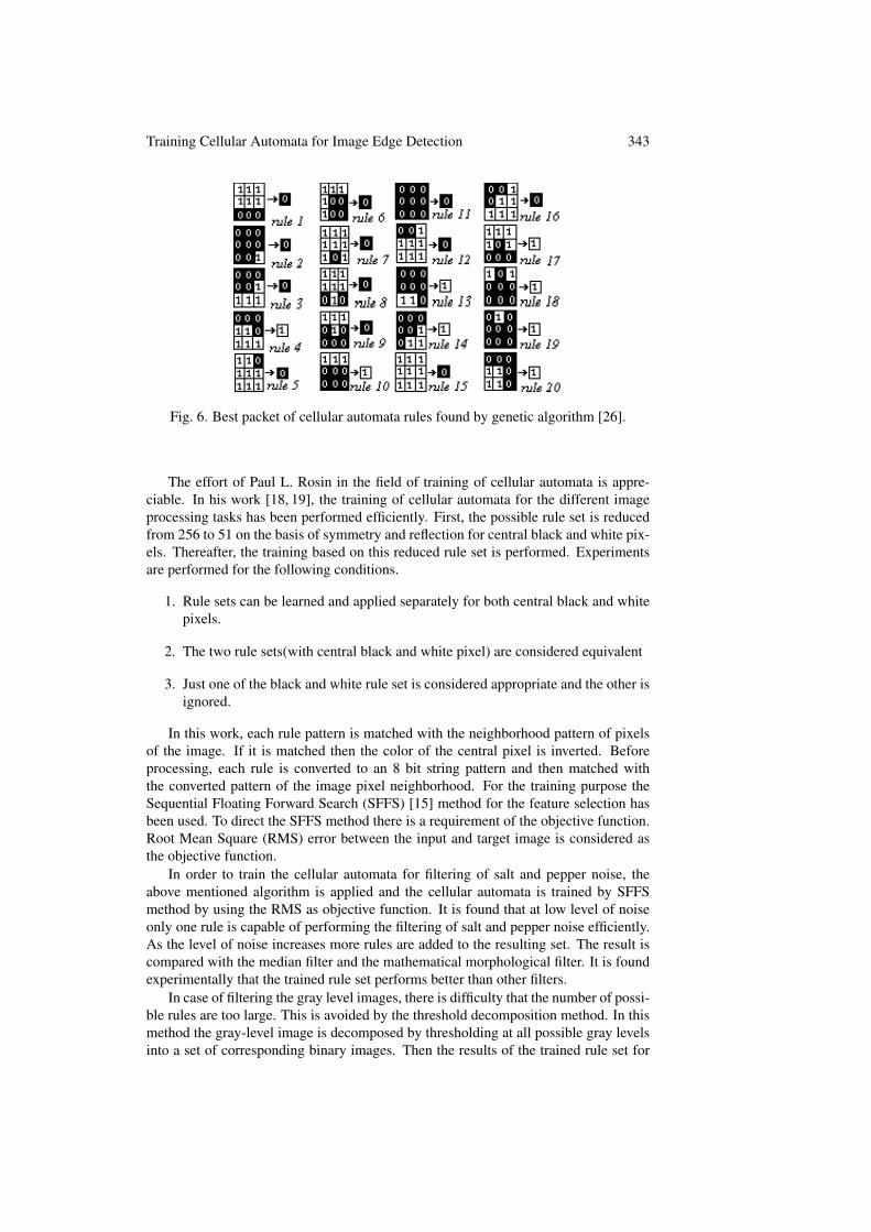
Training Cellular Automata for Image Edge Detection 343
Fig. 6. Best packet of cellular automata rules found by genetic algorithm [26].
The effort of Paul L. Rosin in the field of training of cellular automata is appre-ciable. In his work [18, 19], the training of cellular automata for the different imageprocessing tasks has been performed efficiently. First, the possible rule set is reducedfrom 256 to 51 on the basis of symmetry and reflection for central black and white pix-els. Thereafter, the training based on this reduced rule set is performed. Experimentsare performed for the following conditions.
1. Rule sets can be learned and applied separately for both central black and whitepixels.
2. The two rule sets(with central black and white pixel) are considered equivalent
3. Just one of the black and white rule set is considered appropriate and the other isignored.
In this work, each rule pattern is matched with the neighborhood pattern of pixelsof the image. If it is matched then the color of the central pixel is inverted. Beforeprocessing, each rule is converted to an 8 bit string pattern and then matched withthe converted pattern of the image pixel neighborhood. For the training purpose theSequential Floating Forward Search (SFFS) [15] method for the feature selection hasbeen used. To direct the SFFS method there is a requirement of the objective function.Root Mean Square (RMS) error between the input and target image is considered asthe objective function.
In order to train the cellular automata for filtering of salt and pepper noise, theabove mentioned algorithm is applied and the cellular automata is trained by SFFSmethod by using the RMS as objective function. It is found that at low level of noiseonly one rule is capable of performing the filtering of salt and pepper noise efficiently.As the level of noise increases more rules are added to the resulting set. The result iscompared with the median filter and the mathematical morphological filter. It is foundexperimentally that the trained rule set performs better than other filters.
In case of filtering the gray level images, there is difficulty that the number of possi-ble rules are too large. This is avoided by the threshold decomposition method. In thismethod the gray-level image is decomposed by thresholding at all possible gray levelsinto a set of corresponding binary images. Then the results of the trained rule set for

344 A. P. Shukla
the binary images is applied to each of the binary images obtained by threshold decom-position. Then the results are combined. In this work the results of filtering the binaryimages are simply added. The advantage of this method is that the result of binaryimage training is used directly. The disadvantage is that the decomposition process is atime taking process. The training of cellular automata for thinning of the black regionhas been also performed in this work [18]. As only the black portion is thinned, ruleswere applied in black pixels only. There are two ways to generate the training data.First, some one pixel wide curves were taken as the target output, and were dilated byvarying amounts to provide the prethinned input. Along with that, some thinned binaryimages by applying the standard thinning algorithm are considered. Both sets of datawere combined to form a composite training input and output image pair. The summedproportions of black pixel errors and white pixel errors was considered as the objectivefunction to drive the SFFS algorithm. The resulting trained rule set contains the sevenrules which are capable of performing the thinning of the black portion. The result iscompared with the standard method by visual inspection and found satisfactory. Alongwith the above mentioned algorithms, Rosin [18] also considered two variants of thecellular automata which are the B-rule cellular automata and 2-cycle cellular automata.The aforesaid problems are also trained for these two variants of cellular automata andthe results are found accordingly.
Similar experiments have also been performed for the training of cellular automatafor noise filtering [21, 24] and morphological operations [22, 23, 25]
3 Training StrategyAn image can be considered as a lattice of cells of two dimensional cellular au-
tomata where each pixel corresponds to the particular cell of the CA. In case of binaryimages, a pixel can acquire one of the two values, i.e. 0 and 1. If we consider theMoore neighborhood of the pixels then 28 i.e. 256 rules are possible for the centralwhite pixel and the same for the central black pixel. By using PolyaBurnside countinglemma [16] this number can be reduced by determining the number of distinct patternsafter removing equivalent symmetric versions. According to this lemma the number ofequivalence classes are
Class =1
P
∑p∈P|Fix(p)| (3)
where Class is the number of equivalence classes, P is a set of permutations of a set A,and Fix(p) is the number of elements of A that are invariant under p.
In case of Moore neighborhood of the pixels, the number of equivalence classes interms of the number of possible pixel values x is defined as
Class =x8 + 2x2 + x4 + 4x5
8(4)
where the terms in the numerator are the 0o rotation (identity) ±90o(two rotations),180o(single), and four rotations corresponding to mirror symmetry through vertical,horizontal, and diagonal lines of reflection. For the binary image where the pixel valuespermitted are only 0 and 1. By putting the value of x as 2, equation 4 gives value 51.Hence, after removing the symmetry the reduced rule set contains 51 rules for centerpixel 1 and similarly 51 rules for center pixel 0. The resulting rule set for center pixel1 is shown in figure 7. The same set can be obtained for the center pixel 0 by replacing
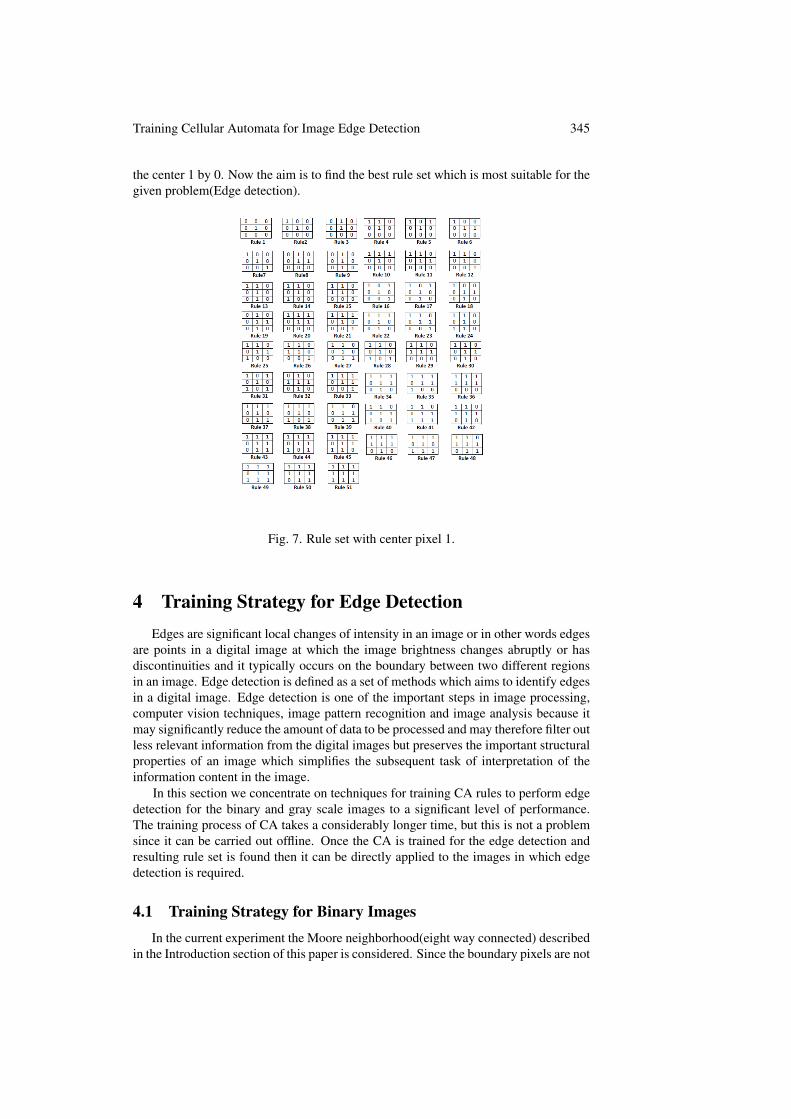
Training Cellular Automata for Image Edge Detection 345
the center 1 by 0. Now the aim is to find the best rule set which is most suitable for thegiven problem(Edge detection).
Fig. 7. Rule set with center pixel 1.
4 Training Strategy for Edge DetectionEdges are significant local changes of intensity in an image or in other words edges
are points in a digital image at which the image brightness changes abruptly or hasdiscontinuities and it typically occurs on the boundary between two different regionsin an image. Edge detection is defined as a set of methods which aims to identify edgesin a digital image. Edge detection is one of the important steps in image processing,computer vision techniques, image pattern recognition and image analysis because itmay significantly reduce the amount of data to be processed and may therefore filter outless relevant information from the digital images but preserves the important structuralproperties of an image which simplifies the subsequent task of interpretation of theinformation content in the image.
In this section we concentrate on techniques for training CA rules to perform edgedetection for the binary and gray scale images to a significant level of performance.The training process of CA takes a considerably longer time, but this is not a problemsince it can be carried out offline. Once the CA is trained for the edge detection andresulting rule set is found then it can be directly applied to the images in which edgedetection is required.
4.1 Training Strategy for Binary ImagesIn the current experiment the Moore neighborhood(eight way connected) described
in the Introduction section of this paper is considered. Since the boundary pixels are not

346 A. P. Shukla
connected by eight pixels, so these pixels are neglected. This is called the fixed valueboundary condition. The start state of each pixel in the cellular automata is consideredas the pixel value of the input image.
4.2 Algorithm
In order to perform edge detection in the given binary image each rule set is consid-ered among 51 rules shown in figure 7. The matching of the pattern is performed only inthe white portion of the given image. Each pixel of the image is taken under considera-tion and if the neighborhood pattern(Moore neighborhood) is matched with the patternof rule or set of rules under consideration then the central pixel is inverted to black,otherwise it remains unaltered. The black portion of the image remains unchanged.One of the challenges is to simulate the parallel behavior of the cellular automata in thesequential machine with a single processor and sequential operations. To resolve thisissue the algorithm is designed in such a manner that in each iteration, all the imagepixels are notionally processed in parallel. To perform this the processed pixels arestored in a secondary image instead, and then copied back to the original image at theend of each iteration. The pseudo code for this algorithm is given in algorithm 1.
Algorithm 1 Edge Detection Using CA Rules
Require: input image of size M ×N , Ruleset1: [row, column]← size(A)2: for i = 2 to M − 1 and j = 2 to N − 1 do3: for k = 1 to 4 do4: if A[i,j] = 1 and 3x3pattern(A[i,j]) = Rotate90o(Rule matrix) then5: C[i, j]← 06: else7: C[i, j]← 18: end if9: end for
10: end for11: B ← C
In the algorithm 1 first, the rule set under consideration is taken into set RuleMatrixwhich is a set of 3x3 matrix. Then for each pixel in image with value 1, the 3x3neighborhood of the pixel is converted into the matrix format. If this pattern is matchedwith the rules under consideration then the value of central pixel is inverted to zero.Otherwise it remains unchanged. The same steps are performed for rotating the 3x3neighborhood pattern to four times each by 90o so that the symmetric patterns can alsobe considered.
4.3 Computational Complexity
Even without the specialized hardware implementations that are available as [14],[28] and [7], the running time of the cellular automata is moderate. If there are N num-ber of pixels, and a neighborhood size of M(here M=8 in case of Moore neighborhood),and K is the number of rules in the rule set, the computational complexity is O(MN).Note that the complexity is independent of the number of rules available in the Ruleset.

Training Cellular Automata for Image Edge Detection 347
4.4 Sequential Floating Forward Search MethodSequential Floating Forward Search (SFFS) [15] is a deterministic feature selec-
tion method and is very widely being used for building classifier systems. The reasonbehind using the SFFS method is
1. Its simplicity of implementation
2. It is deterministic(not randomize) and repeatable.
3. It provides good speed with effectiveness.
4. It does not require the many parameters as necessary for genetic algorithms. [5]
In the past some studies have compared the effectiveness of SFFS against otherstrategies for feature selection. For example, Jain and Zongker [9] found that the SFFSperformed best among the fifteen feature selection algorithms including genetic algo-rithm. Some other studies such as Hao et. al [8] found, in their experiments on differentdata sets, that there was little difference in effectiveness between genetic algorithmsand SFFS.
Algorithm 2 Sequential Floating Forward Search
1: Step 1:2: Y ← {φ}3: Step 2:4: Select the best feature5: x+ ← argmaxJ(Yk + x)|x /∈ Yk6: Yk ← Yk + x+
7: k=k+18: Step 3:9: Select the worst feature
10: x− ← argmaxJ(Yk − x)|x ∈ Yk11: Step 4:12: if J(Yk − x−) > J(Yk) then13: Yk ← Yk − x−14: k = k + 115: Go to Step 316: else17: Go to Step 218: end if
The SFFS algorithm can be described as follows. Let Yk denote the rule set atiteration k and its score be J(Yk). Here, J(Yk) is defined by the result of the algorithm1 by applying the CA rule set to the input image and computing the objective functiondefined in the next subsection. Step 1 shows that the initial rule set is empty. In step2 of each iteration, all rules in figure 7are considered for addition to the rule set. Onlythe rule giving the maximum score is added to the resulting rule set. This process isrepeated until no improvement in score is gained by adding rules. In step 3, each rulein the rule set found in step 2 is removed to find the rule whose removal provides theresulting rule set with the improved value of objective function. As shown in step 4, ifremoval of a rule causes the better score of the objective function then it is discardedfrom the rule set and again the next rule is tried for the deletion and the process goes to

348 A. P. Shukla
step 3. Otherwise, the process goes to step 2 for the addition of a new rule to the ruleset.
4.5 Objective FunctionThe objective function used to select the best rule set has a very crucial role. The
simplest and most used objective function is Mean Square Error(MSE) or the RootMean Squared (RMS) error between the processed and the reference image. However,it has some limitations [6] and they often do not capture the similarity seen by thehuman visual system(HVS). Wang et al. [29] proposed a method for image quality as-sessment which is Structural Similarity Index Measure(SSIM) which measures imagesimilarity taking luminance, contrast and structure into account. But in case of edgedetection even the SSIM index fails to detect edges since the SSIM index is more sen-sitive to the qualitative difference in the edge magnitude map that the CA is capableof producing. The misclassification error defined by Yasnoff et al. [30] has been con-sidered which is best suited for the classification of the edge and non edge pixels. Themisclassification error is defined as
error = 1− |NEo ∩NET |+ |Eo ∩ ET |NEo + Eo
(5)
where Eo and NEo show the edge and non edge pixels of the edge image obtainedby the CA rule where as ET and NET shows the target image which is considered asthe reference image for the purpose of computation.
One of the major issues for checking the performance is to select the target imagewith which the comparison of results is to be made. Since the effectiveness of the al-gorithm depends on the target image hence its role is very important. In the case ofbinary images, the images generated by the Canny edge detector [3] are used as it is awell known optimal edge detector having the property of low error rate, good localiza-tion(The distance between edge pixels detected and real edge pixels is minimum) andminimal response(only one detector response per edge).
So, to find the objective function defined in equation 5 first, the edges of the givenimage are obtained by the Canny edge detector and the resulting image is consideredas the reference image. Then the rule set is applied to the same image to obtain theresulting edge image. Then misclassification error between the reference image andthe edge image obtained by the rule set is calculated. This error is used to drive theSFFS algorithm to find the best rule set for edge detection.
5 Training Strategy for Gray Scale ImagesIn case of gray scale images the training process is very much complicated. In case
of Moore neighborhood where cells can have 256 possible intensities, 2568 neighbor-hood patterns are possible for the central pixel with value 0. Also the same numberof patterns for the central pixel with other values (1 to 255). If we reduce the numberof rules from the rule set by using equation 4, still the number of classes are greaterthan 2 × 10¹⁸, which is obviously too large to enumerate practically. One idea is thatif the given gray scale image is converted to the binary level by threshold decompo-sition then the result of the previous section can be applied for the resulting image.Rosin [18] used the threshold decomposition for all possible gray level values and thencombined the results of each decomposition to find the final image. This method works

Training Cellular Automata for Image Edge Detection 349
for the denoising and other methods but its effectiveness in case of edge detection issuspicious. Also, it is a very time taking process.
To over come the aforesaid problem, we propose a novel method to decomposethe gray level image by Otsu’s threshold decomposition method [13]. The motivationbehind using the Otsu’s method is
1. It is based on a very simple idea: Find the threshold that minimizes the weightedwithin-class variance.
2. This turns out to be the same as maximizing the between-class variance.
3. It is fast
4. It operates directly on the gray level histogram.
Due to the property of minimizing the within class variance and maximizing thebetween class variance Otsu’s method is able to show the maximum objects present inthe image into the thresholded image.
5.1 Otsu’s Thresholding MethodOtsu’s thresholding method is used to automatically perform clustering-based im-
age thresholding in order to convert the gray scale image into a binary image. Thealgorithm assumes that the image contains two classes of pixels following a bi-modalhistogram (foreground pixels and background pixels), it then calculates the optimumthreshold separating the two classes so that their combined spread (intra-class variance)is minimal, or equivalently their inter-class variance is maximal.
Let the weighted sum of variances of the two classes be defined as:
σ2w(t) = w0(t)σ
20(t) + w1(t)σ
21(t) (6)
where, weightsw0 andw1 are the probabilities of the two classes separated by a thresh-old t and σ2
0 and σ21 are the variances of these two classes.
The class probability w0(t) and w1(t) is computed from the L histograms as:
w0(t) =
t−1∑i=0
p(i)
w1(t) =
L−1∑i=t
p(i)
Otsu shows that minimizing the intra-class variance is the same as maximizing theinter-class variance which is expressed in terms of class probabilities w and class meansµ .
σ2b (t) = σ2−σ2
w(t) = w0(µ0−µT )2+w1(µ1−µT )
2 = w0(t)w1(t) [µ0(t)− µ1(t)]2
(7)where, the class mean µ0(t), µ1(t) and µT (t) is defined as:

350 A. P. Shukla
µ0(t) =
t−1∑i=0
ip(i)
w0
µ1(t) =
L−1∑i=t
ip(i)
w1
µT =
L−1∑i=0
ip(i)
The class means and class probabilities can be computed iteratively. The steps ofOtsu’s thresholding is shown in algorithm 3
Algorithm 3 Otsu’s Thresholding Algorithm
1: Compute histogram and probabilities of each intensity level2: Set up initial wi(0) and µi(0)3: For all possible thresholds t=1,. . . maximum intensity do
Update wi and µi
Compute σ2b (t)
4: Desired threshold corresponds to the maximum σ2b (t)
To select the reference image for the calculation of the misclassification error whichis used as the objective function for the gray scale images, images from the Universityof South Florida data set which contains images along with manually generated groundtruth edges [2] are considered. The reference images are dilated first because there maybe a possibility of some positional error in the ground truth edges (which are one pixelwide).
6 Experiments and ResultsIn order to perform the experimental work and the validation of the results, the
whole process is divided into two major parts. First, the training of cellular automatawas done for the binary images and the best rule set for edge detection was learnt.Second, the training was performed for the gray scale images. Then the training pro-cess is applied to the test images and results are verified. To perform the experimentMATLAB 2014a environment has been used for the simulation purpose.
6.1 Training Rule Set for Binary ImageIn order to train the rule set 20 binary sample images are carefully selected in such
a way that the images contain all kind of shapes such as lines, circles, cones and somecomplicated structures. Edges of all selected images are obtained by Canny’s edgedetector and these edge images are considered as reference images. Then the rules areselected by using the objective function misclassification error with reference to theseimages. The Sequential Floating Forward Search(SFFS) method as described in theprevious section was used for the training purpose. In all the images the trained ruleset which gives the best edge detection result is rule number 51 as shown in figure 8.It should be noted that the rule set that was generated in figure 8 is simple, consistingof only one rule. The careful analysis of the rule shows that in the white portion of the

Training Cellular Automata for Image Edge Detection 351
image any pixel in a 3× 3 neighborhood has all pixels white then it inverts the centralpixel to black. Since in our algorithm of the CA the rule is only applied to white pixels,then all white pixels are replaced by black except for pixels adjacent to black pixels inthe input image. This leaves a black image with a one pixel wide white edges.
Fig. 8. Rule set learned for edge detection
The learned rule is applied to 20 binary images and the results are analyzed. Theresult is also compared with some standard edge detector operators such as Roberts,Sobel, Prewitt, Laplacian of Gaussian(LoG) and with Canny edge detectors. The re-sults are shown in figure 9. Note that in the figures shown all edge maps are invertedand figures are scaled down for display purposes. In the current section only results oftwo images are shown.
(a) Original Image (b) LoG Edge Detector
(c) Canny Edge Detector (d) Rule Set Edge Detector
Fig. 9. Results of Edge Detectors

352 A. P. Shukla
The careful observation of the results by visual inspection shows that the trainedrule set which contains only one rule is capable of detecting edges very efficiently.Also, its result is superior than other edge detectors. It performs well in junction whileother edge detectors like Canny edge detector fail to show the sharp edges at junctions.This is shown in figure 9.
It is clearly depicted in figure 9 that the performance of rule set at the corner issuperior than the canny and LoG operator. Both of these operators are not able to showthe junction properly. So, the learnt rule set is capable of detecting the edges whereasmost of the traditional methods fail.
6.2 Training Rule Set for Gray Scale ImagesIn order to train the cellular automata for the gray scale images, 12 images from
the University of South Florida data set which contains images along with manuallygenerated ground truth edges are taken as reference images. As described in the pre-vious section (training strategy for gray scale image) the selected image is thresholdedto convert in binary image by the Otsu’s threshold decomposition algorithm. For thedisplay purpose, the given edge image is inverted before using it as the reference imagesince it is the inverted version of original image. As we know that after threshold de-composition the image is converted to binary and we may directly use the result of thetraining result of binary image. But for satisfaction, the same experiment is again per-formed with the ground truth images as reference image and as expected, the learnedrule set is same i.e., the rule number 51 as shown in figure 8.
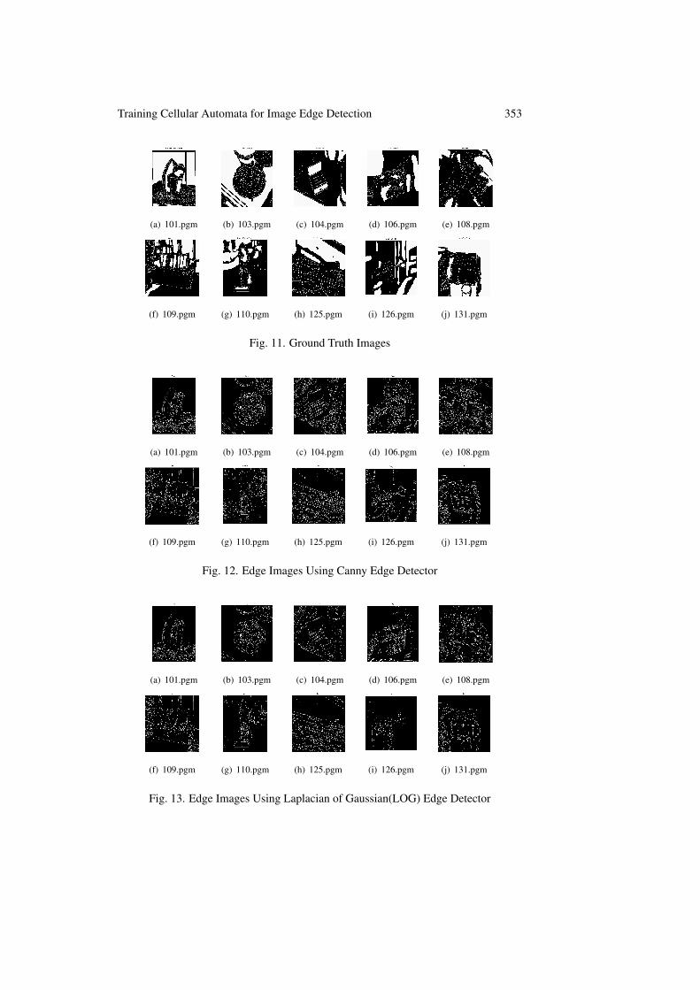
The learned rule is applied to 10 ground truth images and the objective function(misclassification error) is calculated. The results of edge detection using the variousstandard edge detectors are found. Figure 10 shows the original sample images. Figure11 shows the ground truth images showing the edges of the images shown in figure 10.Images of figure 11 are used as reference images and the misclassification errors arecalculated with reference to these images.
(a) 101.pgm (b) 103.pgm (c) 104.pgm (d) 106.pgm (e) 108.pgm
(f) 109.pgm (g) 110.pgm (h) 125.pgm (i) 126.pgm (j) 131.pgm
Fig. 10. Original Images
Training Cellular Automata for Image Edge Detection 353
(a) 101.pgm (b) 103.pgm (c) 104.pgm (d) 106.pgm (e) 108.pgm
(f) 109.pgm (g) 110.pgm (h) 125.pgm (i) 126.pgm (j) 131.pgm
Fig. 11. Ground Truth Images
(a) 101.pgm (b) 103.pgm (c) 104.pgm (d) 106.pgm (e) 108.pgm
(f) 109.pgm (g) 110.pgm (h) 125.pgm (i) 126.pgm (j) 131.pgm
Fig. 12. Edge Images Using Canny Edge Detector
(a) 101.pgm (b) 103.pgm (c) 104.pgm (d) 106.pgm (e) 108.pgm
(f) 109.pgm (g) 110.pgm (h) 125.pgm (i) 126.pgm (j) 131.pgm
Fig. 13. Edge Images Using Laplacian of Gaussian(LOG) Edge Detector
354 A. P. Shukla
(a) 101.pgm (b) 103.pgm (c) 104.pgm (d) 106.pgm (e) 108.pgm
(f) 109.pgm (g) 110.pgm (h) 125.pgm (i) 126.pgm (j) 131.pgm
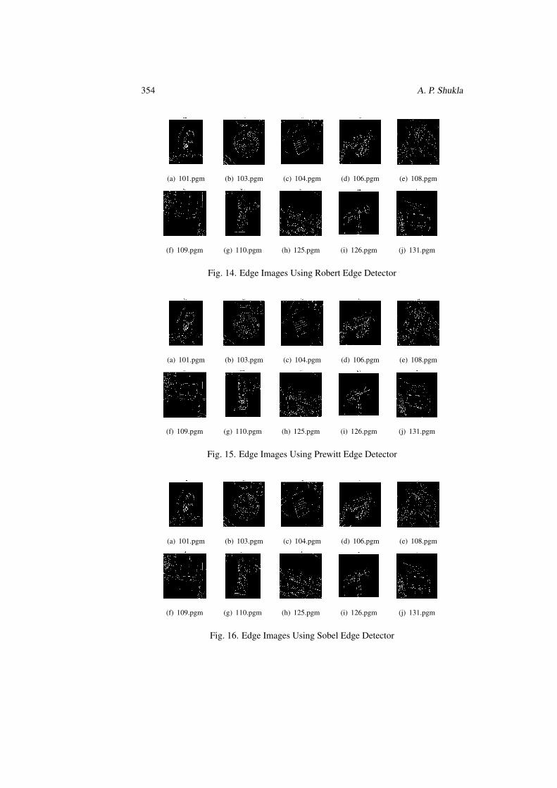
Fig. 14. Edge Images Using Robert Edge Detector
(a) 101.pgm (b) 103.pgm (c) 104.pgm (d) 106.pgm (e) 108.pgm
(f) 109.pgm (g) 110.pgm (h) 125.pgm (i) 126.pgm (j) 131.pgm
Fig. 15. Edge Images Using Prewitt Edge Detector
(a) 101.pgm (b) 103.pgm (c) 104.pgm (d) 106.pgm (e) 108.pgm
(f) 109.pgm (g) 110.pgm (h) 125.pgm (i) 126.pgm (j) 131.pgm
Fig. 16. Edge Images Using Sobel Edge Detector
Training Cellular Automata for Image Edge Detection 355
(a) 101.pgm (b) 103.pgm (c) 104.pgm (d) 106.pgm (e) 108.pgm
(f) 109.pgm (g) 110.pgm (h) 125.pgm (i) 126.pgm (j) 131.pgm
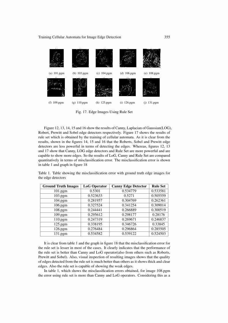
Fig. 17. Edge Images Using Rule Set
Figure 12, 13, 14, 15 and 16 show the results of Canny, Laplacian of Gaussian(LOG),Robert, Prewitt and Sobel edge detectors respectively. Figure 17 shows the results ofrule set which is obtained by the training of cellular automata. As it is clear from theresults, shown in the figures 14, 15 and 16 that the Roberts, Sobel and Prewitt edgedetectors are less powerful in terms of detecting the edges. Whereas, figures 12, 13and 17 show that Canny, LOG edge detectors and Rule Set are more powerful and arecapable to show more edges. So the results of LoG, Canny and Rule Set are comparedquantitatively in terms of misclassification error. The misclassification error is shownin table 1 and graph in figure 18
Table 1. Table showing the misclassification error with ground truth edge images forthe edge detectors
Ground Truth Images LoG Operator Canny Edge Detector Rule Set101.pgm 0.5301 0.534779 0.533581103.pgm 0.523633 0.5271 0.505559104.pgm 0.281957 0.304769 0.262361106.pgm 0.327524 0.341254 0.309014108.pgm 0.244441 0.266889 0.300519109.pgm 0.295612 0.298177 0.28176110.pgm 0.247319 0.269671 0.246837125.pgm 0.338195 0.346726 0.33845126.pgm 0.276484 0.296864 0.285505131.pgm 0.534582 0.539122 0.524503
It is clear from table 1 and the graph in figure 18 that the misclassification error forthe rule set is lesser in most of the cases. It clearly indicates that the performance ofthe rule set is better than Canny and LoG operator(also from others such as Roberts,Prewitt and Sobel). Also, visual inspection of resulting images shows that the qualityof edges detected from the rule set is much better than others as it shows thick and clearedges. Also the rule set is capable of showing the weak edges.
In table 1, which shows the misclassification errors obtained, for image 108.pgmthe error using rule set is more than Canny and LoG operators. Considering this as a

356 A. P. Shukla
Fig. 18. Misclassification Errors for Various Images.
special case some discussion is required.
(a) Original Image (b) Ground Truth Edges (c) LoG Edge Detector
(d) Canny Edge Detector (e) Rule Set Edge Detector
Fig. 19. Results of Edge Detectors for 108.pgm
The results of this image are shown in figure 19 and the justification of the resultis as follows: The ground truth edge images have limitations, as these images aregenerated manually, only strong edges are shown. By the visual inspection of theresults shown in figure 19(e) it is clear that the misclassification error is because ofthe weak edges obtained by the rule set edge detector while they are missing from themanually generated ground truth image. Though the Canny operator also shows theweak edges as shown in figure 19(d), but it is the property of the the Canny operator thatit shows only those weak edges which are connected with the strong edges whereas therule set along with the above mentioned edges, also shows the weak edges that are notconnected with the strong edges. This is the reason of getting more misclassificationerror in the case of edges obtained by the cellular automata rule set.

Training Cellular Automata for Image Edge Detection 357
7 ConclusionsIn this paper the training of cellular automata for edge detection has been per-
formed. The results are encouraging. It has been observed that it is possible to learngood rule sets to perform some complicated image processing tasks such as edge detec-tion. In the case of edge detection the learned rule set is extremely simple as it containsonly a single rule with the performance and efficiency up to the mark. The result of thelearned rule set has also been compared with some standard edge detectors and it hasbeen found that in most of the cases its performance is better than the standard edgedetectors, specially in corner detection. It is important to mention that the aim of cel-lular automata is to provide simplicity to perform the complex tasks, which is clearlydepicted in this paper. As the detection of edges depends on the sensitivity of Otsu’salgorithm, in future some other algorithms may be used in place of Otsu’s algorithmin which there is a provision of sensitivity control which can control the generation ofweak edges as per requirements.
References[1] ANDRE, D., BENNETT III, F. H., AND KOZA, J. R. Discovery by genetic
programming of a cellular automata rule that is better than any known rule for themajority classification problem. In Proceedings of the First Annual Conferenceon Genetic Programming (1996), MIT Press, pp. 3–11.
[2] BOWYER, K., KRANENBURG, C., AND DOUGHERTY, S. Edge detector evalu-ation using empirical roc curves. In Computer Vision and Pattern Recognition,1999. IEEE Computer Society Conference on. (1999), vol. 1, IEEE.
[3] CANNY, J. A computational approach to edge detection. Pattern Analysis andMachine Intelligence, IEEE Transactions on, 6 (1986), 679–698.
[4] COVER, T. M., AND VAN CAMPENHOUT, J. M. On the possible orderingsin the measurement selection problem. Systems, Man and Cybernetics, IEEETransactions on 7, 9 (1977), 657–661.
[5] GOLDBERG, D. E., AND DEB, K. A comparative analysis of selection schemesused in genetic algorithms. Foundations of genetic algorithms 1 (1991), 69–93.
[6] GUO, L., AND MENG, Y. What is wrong and right with mse. In Eighth IASTEDInternational Conference on Signal and Image Processing (2006), pp. 212–215.
[7] HALBACH, M., AND HOFFMANN, R. Implementing cellular automata in fpgalogic. In Parallel and Distributed Processing Symposium, 2004. Proceedings.18th International (2004), IEEE, p. 258.
[8] HAO, H., LIU, C.-L., AND SAKO, H. Comparison of genetic algorithm andsequential search methods for classifier subset selection. In ICDAR (2003), Cite-seer, pp. 765–769.
[9] JAIN, A., AND ZONGKER, D. Feature selection: Evaluation, application, andsmall sample performance. Pattern Analysis and Machine Intelligence, IEEETransactions on 19, 2 (1997), 153–158.

358 A. P. Shukla
[10] JIMENEZ MORALES, F., CRUTCHFIELD, J. P., AND MITCHELL, M. Evolvingtwo-dimensional cellular automata to perform density classification: A report onwork in progress. Parallel Computing 27, 5 (2001), 571–585.
[11] JUILLE, H., AND POLLACK, J. B. Coevolving the” ideal” trainer: Applicationto the discovery of cellular automata rules. In University of Wisconsin (1998),Citeseer.
[12] MITCHELL, M., CRUTCHFIELD, J. P., AND HRABER, P. T. Evolving cellularautomata to perform computations: Mechanisms and impediments. Physica D:Nonlinear Phenomena 75, 1 (1994), 361–391.
[13] OTSU, N. A threshold selection method from gray-level histograms. Automatica11, 285-296 (1975), 23–27.
[14] PRESTON, K., AND DUFF, M. J. Modern cellular automata: theory and appli-cations, vol. 198. Plenum Press New York, 1984.
[15] PUDIL, P., NOVOVICOVA, J., AND KITTLER, J. Floating search methods infeature selection. Pattern recognition letters 15, 11 (1994), 1119–1125.
[16] ROBERTS, F., AND TESMAN, B. Applied combinatorics. CRC Press, 2011.
[17] ROSIN, P., ADAMATZKY, A., AND SUN, X. Cellular Automata in Image Pro-cessing and Geometry, vol. 10. Springer, 2014.
[18] ROSIN, P. L. Training cellular automata for image processing. Image Processing,IEEE Transactions on 15, 7 (2006), 2076–2087.
[19] ROSIN, P. L. Image processing using 3-state cellular automata. Computer visionand image understanding 114, 7 (2010), 790–802.
[20] SAHOTA, P., DAEMI, M., AND ELLIMAN, D. Training genetically evolvingcellular automata for image processing. In Speech, Image Processing and NeuralNetworks, 1994. Proceedings, ISSIPNN’94., 1994 International Symposium on(1994), IEEE, pp. 753–756.
[21] SHUKLA, A. P., AND AGARWAL, S. Training cellular automata for salt andpepper noise filtering. In Computational Intelligence on Power, Energy and Con-trols with their impact on Humanity (CIPECH), 2014 Innovative Applications of(2014), IEEE, pp. 519–524.
[22] SHUKLA, A. P., AND AGARWAL, S. Training two dimensional cellular automatafor some morphological operations. In Computational Intelligence on Power,Energy and Controls with their impact on Humanity (CIPECH), 2014 InnovativeApplications of (2014), IEEE, pp. 121–126.
[23] SHUKLA, A. P., AND AGARWAL, S. Selection of optimum rule set of two di-mensional cellular automata for some morphological operations.
[24] SHUKLA, A. P., CHAUHAN, S., AND AGARWAL, S. Training of cellular au-tomata for image filtering. In Proc. Second International Conference on Advancesin Computer Science and Application-CSA 2013 (2013), pp. 86–95.

Training Cellular Automata for Image Edge Detection 359
[25] SHUKLA, A. P., CHAUHAN, S., AGARWAL, S., AND GARG, H. Training cel-lular automata for image thinning and thickening. In Confluence 2013: TheNext Generation Information Technology Summit (4th International Conference)(2013), IET, pp. 394–400.
[26] SLATNIA, S., AND KAZAR, O. Images segmentation based contour using evcaapproach, evolutionary cellular automata. Courrier du Savoir, 09 (2009).
[27] SOMOL, P., PUDIL, P., AND KITTLER, J. Fast branch & bound algorithmsfor optimal feature selection. Pattern Analysis and Machine Intelligence, IEEETransactions on 26, 7 (2004), 900–912.
[28] TOFFOLI, T., AND MARGOLUS, N. Cellular automata machines: a new envi-ronment for modeling. MIT press, 1987.
[29] WANG, Z., BOVIK, A. C., SHEIKH, H. R., AND SIMONCELLI, E. P. Imagequality assessment: from error visibility to structural similarity. Image Process-ing, IEEE Transactions on 13, 4 (2004), 600–612.
[30] YASNOFF, W. A., MUI, J. K., AND BACUS, J. W. Error measures for scenesegmentation. Pattern Recognition 9, 4 (1977), 217–231.