i  

  

ii  

 

The production of this Training Manual was made possible by funding from the Asia-Pacific Network (APN) for Global Change Research under the CaPaBle Programme. Reproduction of part or all of this manual is not allowed without permission by the authors or the MSUNFSTDI. All Rights Reserved.

Recommended Citation:

De Guzman, A.B., R.A. Abrea, C.L. Nañola, and W.H. Uy. 2010. Training Manual for Monitoring Marine Protected Areas in the Asia-Pacific Region. Published by MSU Naawan and MSUNFSTDI, with funding from the Asia-Pacific Network for Global Change Research (APN) under the CaPaBle Programme. 66 p.

Cover Design by Ramon Francisco Padilla & Rustan C. Eballe

Photo Credits:

Front Cover: Aerial photo by Paul Chesley (National Geographic, 2009); photos of coral reefs by Renoir Abrea; photo of mangrove by Jerry Garcia; and photo of seagrass by Wilfredo Uy.

Back Cover: All photos on coral reefs by Renoir Abrea; photo on sardine shoal in Cebu (third from left) by Michael Barrow (2010); and photo on blue tunicate by Wilfredo Uy.

 

M

of

onito

D

Capacf Marin

for Cli

The As

C

oringIn the

De Guzm

city Buile Proteimate C

sia-PacifiUnd

MSU NaaTec

MindanNaa

enter for CBo

Mare Asia

A Trai

man

lding focted Ar

Change

A Projic Networder the C

Impleawan Fouchnology

nao Stateawan, Misam

In CollabCoastal an

ogor AgriBog

ine P-Paciining M

Abrea

or Researeas: An in the A

ject Funderk for GloaPaBle P

emented byundation y Develop

and e Universmis Orienta

boration wnd Marinecultural U

gor, Indones

2010

Protecfic Re

Manual

Nañ

arch andn AdaptAsia-Pa

d by obal ChanProgramm

y the for Scien

pment, In

sity at Naal, Philippine

ith the e ResourcUniversitsia

cted egion

ñola

d Monitoive Mec

acific Re

nge Reseme

nce and c.

awan es

ce Studiesy

Area

Uy

oring chanismegion

earch

s

i 

as

m

  

ii  

Monitoring Marine Protected Areas In the Asia-Pacific Region: A Training Manual

Asuncion Biña De Guzman, PhD Renoir A. Abrea Cleto M. Nañola Wilfredo H. Uy, Ph.D.  

2010

Printed in Naawan, Misamis Oriental, Philippines

Authors’ Affiliations

Asuncion Biña De Guzman, Ph.D. Professor, Mindanao State University at Naawan and APN Project Leader

Renoir A. Abrea Professor, Mindanao State University at Naawan

Cleto M. Nañola Assistant Professor, UP Mindanao

Wilfredo H. Uy, Ph.D. Professor and Director of Research, Mindanao State University at Naawan

Recommended Citation:

De Guzman, A.B., R.A. Abrea, C.L. Nañola, and W.H. Uy. 2010. Training Manual for Monitoring Marine Protected Areas in the Asia-Pacific Region. Published by MSU Naawan and MSUNFSTDI, with funding from the Asia-Pacific Network for Global Change Research (APN) under the CaPaBle Programme. Naawan, Misamis Oriental, Philippines. 66p.

The production of this Training Manual was made possible through funding support from the Asia-Pacific Network (APN) for Global Change Research under the CaPaBle Programme under the terms and conditions of CBA2010-11NSY-DeGuzman. Reproduction of part or all of this manual is not allowed without permission by the authors or the MSUNFSTDI. All Rights Reserved.

  

iii  

 

 

 

Introduction

Marine Protected Areas as Adaptive Mechanisms for Global Change 

Strategic goals of MPAs Importance of MPA Monitoring: Ecological, economic and governance perspectives 

What is Monitoring? 

Project goals and objectives 

MPA Database in the Asia‐Pacific Region 

1

24

45

Module 1  Monitoring Coral Reefs and Other Macrobenthos in MPAs Coral reef diversity Status of coral reefs in the Asia‐Pacific  Tools and Techniques in Monitoring Coral Reefs Considerations in long‐term coral monitoring Monitoring impacts of climate change and other environmental events Coral Bleaching and Climate Change Coral Diseases  Drawing up a Monitoring Plan 

6

610102526

283037

Module 2  Monitoring Fish Communities Reef fish diversity Status of Philippine coral reef fishes Methods of Reef fish Monitoring  

39394142

Module 3  Monitoring Seagrass Communities Assessment Methods Data Processing  

495054

Module 4  MangroveEcosystems Mangrove Communities: their role in ecosystem interconnectivity Status of mangrove resources in the Asia‐Pacific region Methods in mangrove assessment Data management and analysis  

5858

60

6063

References   65

                               contents

1  

Introduction

PROJECT RATIONALE AND TRAINING OBJECTIVES

Marine Protected Areas as Adaptive Mechanisms for Global Change  

Conventional methods of  regulating  fisheries,  such  as effort  and  gear  restrictions, limited access to a fishing ground or constraints on catch, have often failed to prevent the continuous  depletion  of  fish  stocks  (De Guzman  2004a). Shifting  paradigms  in  fisheries management  have  been  initiated  by  public  concern  about  ecosystem  integrity,  which accounts for the fact that “fishing always does more than catch the target fish” (Walters et al., 1998).   Despite their global  importance marine ecosystems are by  far the  least known among  the ecosystems  in  the world, especially  in developing countries where  research  is often not a priority  (Cheung et al 2002). Although new species continue  to be discovered worldwide  updated  information  on  marine  biodiversity  in  Southeast  Asia  is  especially scarce. This region, which  is considered an area of highest marine biodiversity,  is also the most seriously threatened (Burke et al 2002).   

Coastal marine  habitats  are  being  exploited  beyond  their  capacity  to  recover  as overfishing  and  destruction  of  coral  reef,  mangroves,  seagrass,  and  estuarine  habitats continue  (White  et  al.  2006).  The  coastal  zone  sustains  a  wide  array  of  impacts  from increasing diversity of economic activities (Figure 1), many of them are not sustainable.  In the  Philippines,  reducing  fishing  pressure  and  habitat  destruction  are  considered  critical management  strategies  and  often means  providing  alternative  source  of  livelihood  and income.  In many  coastal  communities  tourism  increasingly  supplements or  substitutes as income  source  for  fisherfolk.  On  the  other  hand,  tourism  can  contribute  to  habitat degradation through diver damage on coral reefs and gives rise to additional resource use conflicts  in  the  coastal  zone. Fortunately, everywhere  in  the Asia‐Pacific  region  there has been  a  growing  realization  on  the  need  for maintenance  of  high  biodiversity  levels  and pristine coastal areas because  they prove  to be vital  in attracting and  sustaining  tourism, and in maintaining healthy stocks of fish food (White et al. 2006).  

 

Fig. 1. Varied economic activities and their associated impacts in the coastal zone. (Source: Philippine Coastal Manage‐ment Guidebook Series No. 5, 2001).   

  

2  

The  concept  of marine  protected  areas  (MPAs)  as  a  strategy  in  coastal  resource management (CRM) has gained popularity  in the last two decades. Many local communities of  tropical  countries  have  established marine  reserves  or  fish  sanctuaries  to  ensure  the sustainability of fish stocks, and as an attempt to avert the downtrend of   coastal capture fisheries.    The  creation  of   MPAs  is  probably  the most    appropriate  option  to  protect biodiversity and sustain harvests from the reefs and thus would provide long‐term benefits to    fisherfolk.  In marine  reserves  fish populations can grow and  reproduce unimpeded by  fishing of any kind, attain  larger  sizes and   export    fish biomass  (larvae and adult  fish)  to non‐reserve  areas  that,  consequently,    supplements  surrounding  fisheries  (Holland  & Brazee, 1996). Preservation of genetic diversity through protection also helps maintain the stability and integrity of the coastal ecosystem.  Reserves also provide areas for recruitment of  fish populations and a refuge from adjacent areas that are fished.  

Marine  protected  areas  (MPAs)  ‐    marine  reserves,  marine  parks,  and  fish sanctuaries ‐ achieve protection of particular well‐defined critical habitats and biodiversity hotspots. MPAs, if properly designed and well‐managed, can meet various marine resource and coastal conservation needs by preserving habitats and important species through strict protection  of  specific  areas. Coral  reef  fisheries  in  particular  can  be managed  effectively through  implementation  of  “no  take”  areas within  the  reef  (Roberts  and  Polunin  1993). Leading  conservation  organizations  have  adopted  this  approach  as  primary  objective  in global strategies for conserving biologically important areas (White et al. 2006). 

 Strategic goals of MPAs 

Marine protected areas have multiple goals – all of which are considered strategic in sustaining marine biodiversity and fisheries (De Guzman 2004b): 

Conservation of marine biodiversity and genetic resources 

Protection of adjacent marine habitats (mangroves, seagrass beds & coral reefs) 

Refuge of fish from areas that are fished  

Areas where fish can freely grow to maturity and reproduce  

Help sustain and increase fish catch through protection of breeders and ensuring successful recruitment 

Export of fry and adult fish (“spillover effect”) to fished areas, thus, help prevent fishery collapse (i,.e. “insurance policy”) 

Helps improve fisher income from sustained fish catch  

Marine  protected  areas  promote  ecosystem‐based  management  ‐  a  holistic 

approach  to ensure  the protection of contiguous coastal habitats and conservation of  the 

living resources. Marine protected areas are also considered potential measures for climate 

change  adaptation,  particularly  in  buffering  the  effects  of  coral  bleaching  resulting  from 

increasing ocean temperatures and hastening recovery from both climate‐induced stresses 

and overfishing (Arceo et al. 2002; Aliño et al., 2004). Protecting the high biodiversity inside 

MPAs increases the resilience of coral reefs to climate‐induced environmental disturbance. 

  

3  

Various scales in Marine Protected Areas and MPA Networks 

  Declared and proposed MPAs have been classified as  a) global/regional, b) national,  and c) local priorities, based on the following criteria (Cheung et al. 2002): 

i. the biodiversity and ecological values of the MPAs;  ii. consideration of the existing and potential threats imposed upon them, and  iii. feasibility  of management which  includes  the  social  environment  that  is  a 

determinant in the likelihood success.  

Majority  of  the  global/regional  sites  covers  regional  priority  areas  except  those which  are  internationally  recognized  (e.g.  Tubbataha  Reefs  National Marine  Reserve  as World  Heritage  Site  and  Olango  Island  Wildlfie  Sanctuary  as  RAMSAR  site).    The prioritization process provides guidelines for resource allocation at the  local, national, and international  levels. Although  local MPAs are of  lower priority  in the  international context, they  are essential  in  forming  a healthy network of  sites  for marine  conservation  and  for sustaining fisheries resources for local villagers depend upon them for livelihood (Aliño et al 2000; Aliño et al., 2004). More recent innovations in the MPA concept is the establishment of networks of small MPAs managed by local governments and communities to broaden the scope of protection. MPA networking has been pursued  in many areas of  the Philippines (Aliño 2009), and  is  seen as a  cost‐effective means of  increasing  the  scope of protection  and inter‐LGU cooperation. Potential benefits of the MPA network include the conservation of major marine habitats  and  resources  at  the  regional  level  (Pilcher  2009),  such  as  the protection of marine turtles within the Sulu Sulawesi Seascape (SSS). 

 

Importance of MPA monitoring: Ecological, economic, and governance perspectives 

What is Monitoring? 

Monitoring  is  using  a  standard method  to  observe  one  thing  in  one place  over  a period of time.  Information from monitoring  is  like comparing two pictures of a person or place  taken  at different  times  to  see  if  any  changes have occurred.  Similarly, monitoring collects evidence of changes from which trends may be deduced from a series of pictures and may help predict the direction and speed of future changes (Uychiaoco et al. 2010).   

Project Goals and Training Objectives 

Effective MPA management, however, is constrained by weak monitoring programs due to inadequately trained manpower. Majority of the MPAs established in the Philippines and other parts of Asia do not have a  regular monitoring program,  largely due  to  lack of funds and  technical  staff  to undertake a  regular bio‐physical assessment. Recognizing  the need to build local and regional capacity for MPA monitoring, the Asia‐Pacific Network  for Global Change Research (APN)  is funding the project   “Capacity Building for Research and Monitoring of Marine Protected Areas: An Adaptive Mechanism for Climate Change in the Asia‐Pacific Region” under the CaPaBle Programme. The project seeks to build the capacity 

  

4  

of marine protected area (MPA) managers and technical staff of  local government units  in coral reef‐rich countries particularly in the Asia‐Pacific region.  

Several countries in the Asia‐Pacific region (e.g. Philippines, Indonesia, and Thailand) 

have  considerable  experience  with  establishment  of MPAs  as  adaptive mechanisms  for 

natural  and  anthropogenic  impacts.  The  Philippines  and  Indonesia,  two  of  six member 

states  of  the  Coral  Triangle  Initiative,  have MPAs  that  date  back more  than  30  years. 

Training of MPA monitoring teams will employ scientifically sound research and assessment 

methods of  coral  reef,  seagrass, and mangrove  communities. Developing   a pool of MPA 

researchers and monitoring & evaluation  (M&E) practitioners will hopefully help member 

countries increase their ability to adapt to climate change and human‐induced stresses and 

contribute to the sustainable development of coastal ecosystems in the Asia‐Pacific region. 

The  capability building project  in MPA monitoring  shall be  implemented  at  two  levels:  a 

Local  (Mindanao‐wide)  and  Regional  (selected  Asia‐Pacific  countries)  training  series.  The 

training program targets to train a total of 40 technically capable MPA practitioners within 

the region who, in turn, shall become trainers in their respective countries.    

 

MPA Database in Asia‐Pacific  Region 

Apart from enhancing the ability of MPA monitors in the bio‐physical monitoring of MPAs, the project shall also guide participants in formulating an effective M&E program and in  implementing  it  in their respective areas. Participants will be encouraged to write their monitoring  results  for  presentation  and  feedbacking  to  the  community  and  the  local government. The outputs of these monitoring programs can contribute to building of a MPA database in the Asia‐Pacific region.      

Trainers Tips (adopted from Uychiaoco et al. 2010)

Key Concepts

1. Monitoring and evaluation is essential for management to be responsive to the changes in the biophysical and socioeconomic realities as an area is being managed.

2. Observations must be done in places and times that represent the variations in the places and times of interest.

3. Observe those indicators that address what you want to know. 4. The monitoring plan must be feasible. Though there are many definitions of adaptive management, the basic idea is that management strategies are continuously improved as understanding of the system being managed improves. It is very important that the indicators you decide to monitor are relevant to what the community wants to know. If current use is sustainable under the present management strategy, your indicator must either be stable or changing towards the direction desired (e.g. fish catch is stable or increasing). If you are evaluating management, your indicators must be potentially responsive to management.

  

5  

Module 1 MONITORING OF CORALS AND OTHER

MACROBENTHOS IN MPAs

Coral Reef Diversity

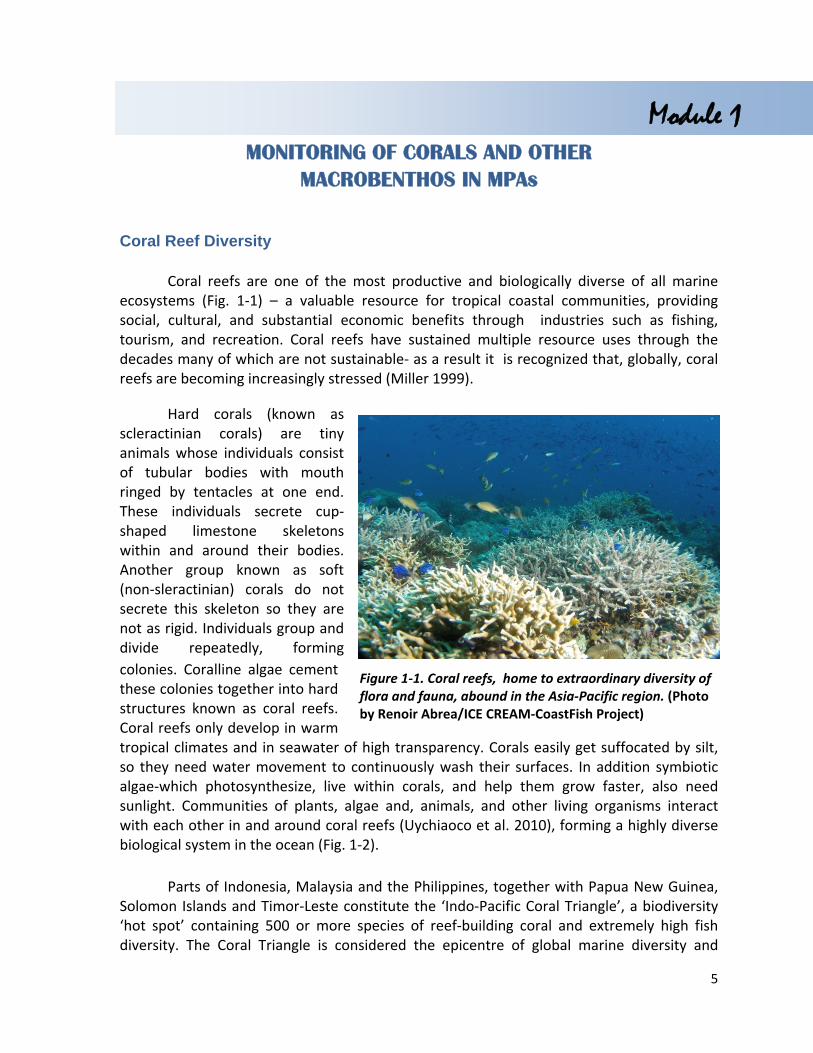
Coral  reefs  are  one  of  the most  productive  and  biologically  diverse  of  all marine ecosystems  (Fig.  1‐1)  –  a  valuable  resource  for  tropical  coastal  communities,  providing social,  cultural,  and  substantial  economic  benefits  through    industries  such  as  fishing, tourism,  and  recreation.  Coral  reefs  have  sustained multiple  resource  uses  through  the decades many of which are not sustainable‐ as a result it  is recognized that, globally, coral reefs are becoming increasingly stressed (Miller 1999).  

Hard  corals  (known  as scleractinian  corals)  are  tiny animals whose  individuals  consist of  tubular  bodies  with  mouth ringed  by  tentacles  at  one  end. These  individuals  secrete  cup‐shaped  limestone  skeletons within  and  around  their  bodies. Another  group  known  as  soft (non‐sleractinian)  corals  do  not secrete  this  skeleton  so  they  are not as rigid. Individuals group and divide  repeatedly,  forming 

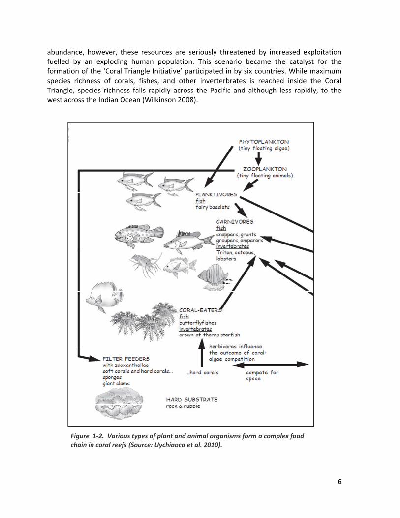
colonies.  Coralline  algae  cement these colonies together into hard structures  known  as  coral  reefs. Coral reefs only develop in warm tropical climates and  in seawater of high transparency. Corals easily get suffocated by silt, so  they need water movement  to continuously wash  their surfaces.  In addition  symbiotic algae‐which  photosynthesize,  live  within  corals,  and  help  them  grow  faster,  also  need sunlight.  Communities  of  plants,  algae  and,  animals,  and  other  living  organisms  interact with each other in and around coral reefs (Uychiaoco et al. 2010), forming a highly diverse biological system in the ocean (Fig. 1‐2).  

Parts of  Indonesia, Malaysia and the Philippines, together with Papua New Guinea, Solomon  Islands and Timor‐Leste constitute the  ‘Indo‐Pacific Coral Triangle’, a biodiversity ‘hot  spot’  containing  500  or more  species  of  reef‐building  coral  and  extremely  high  fish diversity.  The  Coral  Triangle  is  considered  the  epicentre  of  global marine  diversity  and 

Figure 1‐1. Coral reefs,  home to extraordinary diversity of flora and fauna, abound in the Asia‐Pacific region. (Photo by Renoir Abrea/ICE CREAM‐CoastFish Project)  

  

6  

abundance,  however,  these  resources  are  seriously  threatened  by  increased  exploitation fuelled  by  an  exploding  human  population.  This  scenario  became  the  catalyst  for  the formation of the ‘Coral Triangle Initiative’ participated  in by six countries. While maximum species  richness  of  corals,  fishes,  and  other  inverterbrates  is  reached  inside  the  Coral Triangle,  species  richness  falls  rapidly  across  the Pacific  and  although  less  rapidly,  to  the west across the Indian Ocean (Wilkinson 2008).  

 Figure  1‐2.  Various types of plant and animal organisms form a complex food chain in coral reefs (Source: Uychiaoco et al. 2010).  

 

  

7  

Status of Coral Reefs in the Asia-Pacific

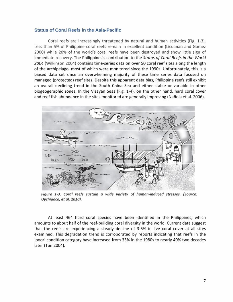
Coral  reefs  are  increasingly  threatened by natural  and human  activities  (Fig.  1‐3). Less  than 5% of Philippine coral  reefs  remain  in excellent condition  (Licuanan and Gomez 2000) while  20%  of  the world’s  coral  reefs  have  been  destroyed  and  show  little  sign  of immediate recovery. The Philippines’s contribution to the Status of Coral Reefs in the World 2004 (Wilkinson 2004) contains time‐series data on over 50 coral reef sites along the length of the archipelago, most of which were monitored since the 1990s. Unfortunately, this is a biased  data  set  since  an  overwhelming  majority  of  these  time  series  data  focused  on managed (protected) reef sites. Despite this apparent data bias, Philippine reefs still exhibit an  overall  declining  trend  in  the  South  China  Sea  and  either  stable  or  variable  in  other biogeogeraphic  zones.  In  the Visayan Seas  (Fig. 1‐4), on  the other hand, hard coral cover and reef fish abundance in the sites monitored are generally improving (Nañola et al. 2006).  

 

 Figure  1‐3.  Coral  reefs  sustain  a  wide  variety  of  human‐induced  stresses.  (Source: Uychiaoco, et al. 2010). 

 

 

At  least  464  hard  coral  species  have  been  identified  in  the  Philippines,  which amounts to about half of the reef‐building coral diversity in the world. Current data suggest that  the  reefs  are  experiencing  a  steady  decline  of  3‐5%  in  live  coral  cover  at  all  sites examined.  This  degradation  trend  is  corroborated  by  reports  indicating  that  reefs  in  the ‘poor’ condition category have increased from 33% in the 1980s to nearly 40% two decades later (Tun 2004).

 

  

8  

 Figure 1‐4. Profile on  live coral (hard and soft)  in the different biogeographical regions of the Philippines (Source: Nañola et al. 2006).   

 

Monitoring  programs  are  essential  in  detecting  changes  in  coral  communities  in 

order to, among others, provide data for making effective management decisions. Given the relatively  high  costs  of  monitoring  programs,  selection  of  the  appropriate  monitoring method for specific objectives is therefore important. Corals and coral reefs are the focus of MPA  protection  because  they  are  less  accessible  to  monitor  and  evaluate  than  either mangrove forests or seagrass beds (Uychiaoco et al. 2010). Because of their naturally high productivity  and  aesthetic  beauty,  coral  reefs  are  more  frequently  the  centerpiece  of Marine  Protected  Areas.  Managing  coral  reefs  will  ensure  the  longevity  of  the  social, economic and ecological benefits  that humans derive  from  them. There  is also a need  to keep  track of  the changes  in  their community structure  (diversity and coral cover)  to  find out whether present use and management are  sustainable or  if  they  could be  improved. Constant monitoring  of  the  reef’s  condition will  also  enable MPA managers  to  respond appropriately in the context of adaptive management. 

Southeast Asia (SEA) contains the largest area of coral reefs with about 100,000 km2 (34%  of  world’s  total).  The  region  is  regarded  as  the  global  centre  of  tropical  marine biodiversity, with 600 hard coral species and more  than 1300  reef‐associated  fish species (Wilkinson 2008). The biodiversity value of Southeast Asian coral reefs is unparalleled in the world with more coral and  fish species than anywhere else  including a high proportion of endemic  species  of  fish,  corals  and  invertebrates. Over‐fishing  and  unsustainable  fishing practices have led to declining fish stocks in almost all SEA countries, pushing many fishers 

  

9  

to  resort  to  destructive  fishing  practices.  Coral  reef monitoring  between  2004  and  2008 indicate  that  reefs  continue  to  show  an  overall  decline  in  condition  in  Indonesia  and Malaysia,  while  there  have  been  slight  improvements  in  the  overall  reef  condition  in Philippines, Singapore and Thailand. The greatest  improvement  in reef condition however, was seen in Vietnam where most reefs in the ‘poor’ category shifted to the ‘fair’ category. 

Tools and Techniques in Monitoring Coral Reefs

The following section describes the most common benthic lifeform survey methods used in baseline assessment and monitoring corals and other macrobenthos on the reef.    

A. Broad‐scale assessment: Manta Tow Reconnaissance Technique 

The  manta  tow  method  has  been  widely  used  in Micronesia  and  the  Great Barrier Reef for assessing broad‐scale changes in reef cover due to cyclone damage, coral bleaching and outbreaks of the crown‐of‐thorns starfish, Acanthaster plancii. A good synopsis of the method is given in English et al (1997) which forms the basis of the following description.  

The manta board  (Fig. 1‐5)  is  attached  to  a motor boat with  a 17 m  length of rope  which  has  buoys  placed  at  distances  of  6 m  and  12 m  from  the  board.  A snorkeller grips the board and  is towed for approximately 2 minutes, at the end of which the boat pauses to allow the surveyor to record data (usually on a plastic slate or water‐resistant paper attached  to  the board). The coverage of bottom  features may be recorded on a percentage scale (for an example, see Fig. 1‐6) or on a scale of 1–5, where 5  indicates  the  greatest  cover  and 0  is used  for  absence. However,  a scale  of  1–5  has  the  short‐coming  that  observers  may  be  tempted  to  place  a disproportionately  large  number  of  values  in  the  middle  category  (i.e.  3),  thus creating  observer  bias.  If  possible,  a  scale  of  1–6  or  1–4  is more  desirable  (see Kenchington 1978).  

 

 

Features of the coral reef which should be amenable to this type of survey  include the following:  

 

Living biotic features  Substrata Others 

live hard corals 

soft corals 

macroalgae 

sponge 

sand

mud 

bedrock 

rubble 

dead coral 

geomorphology 

visibility  

depth   

 

  

10  

Figure 1‐5.   Detail of the manta board and associated equipment. It is recommended that the board be made from marine ply and painted white. Two indented handgrips are positioned towards both front corners of the board and a single handhold is located centrally on the back of the board.    (Redrawn from: English et al. 1997.)

Estimating percent cover

Figure 1-6. Estimating percent cover on the benthos using a metre-square quadrat with string or fishing line strung across at 10 cm intervals. In each example, shaded regions represent different types of substratum that are included collectively in the total percent cover estimate. (Source: Rogers et al 1994.)

B. Line‐Intercept Transect 

Coral  reef  communities  have  been  monitored  using  Line  Intercept  Transect Technique  (LIT),  a method  adopted  by  coral  reef  ecologists  from  terrestrial  plant ecologists  (Loya  1978,  Marsh  et  al  1984,  English  et  al  1994).    The  LIT  method requires  in situ  identification of  the  lifeforms directly under  the  transect  tape. The community is characterized using lifeform categories which provide a morphological description of the reef community. These categories are recorded on data sheets by divers who  swim along  lines which are placed  roughly parallel  to  the  reef crest at depths of 3 meters and 10 meters at each site. For future monitoring, the location of each site is recorded and marked on the reef. If the expertise of the observer allows the  identification  of  coral  species,  this methodology may be  expanded  to  include 

  

11  

taxonomic data  in addition  to  the  lifeform categories. Where possible, monitoring should be repeated each year or at least every two (2) years (English et al. 2007). 

The LIT  is used  to estimate  the cover of an object or group of objects within a specified area by calculating the fraction of the length of the line that is intercepted by  the  object.  This  measure  of  cover,  usually  expressed  as  a  percentage,  is considered to be an unbiased estimate of the proportion of the total area covered by that object, as long as the following assumptions apply: that the size of the object is  small  relative  to  the  length of  the  line;  and  that  the  length of  the  line  is  small relative to the area of interest (English et al. 1997). 

This  technique, however, has  raised  concerns  regarding data quality,  since  the identification of  the  lifeform will be affected by  the observer’s  level of  taxonomic training and factors that may affect the actions or decision of the observer such as bad  weather,  water  currents,  temperature,  or  physical  health.  Another  main limitation  of  the  method  is  the  extended  diver  bottom  time  depending  on  the diversity of the coral community being surveyed (Vergara and Licuanan 2007).   

Logistics needed in LIT (All texts in this section reproduced from IUCN 1993) 

Personnel 

o A team of at least 3 personnel is required ‐ 2 divers and a person in the boat.  

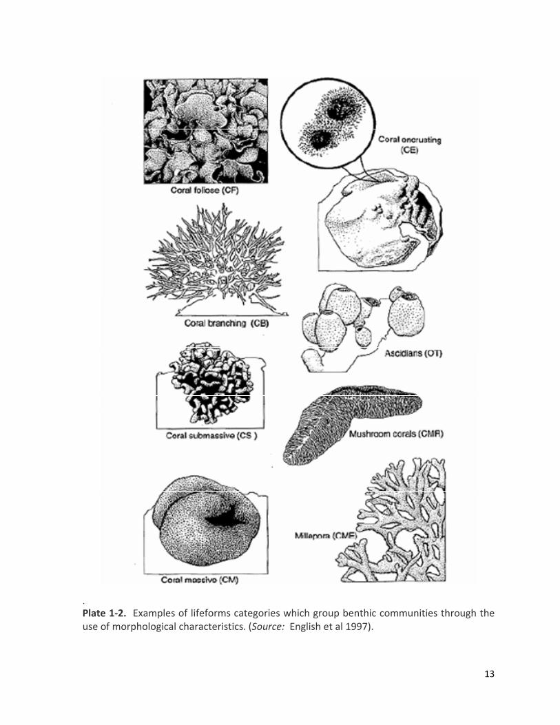
o All  observers  should  be  familiar with  the  definitions  of  each  lifeform  (see Plates  1‐4;  Table  1‐1).  For  example,  branching  forms  are  defined  as  those with at least secondary branching.    

o Training should be carried out  in the field, but may  include the use of slides and/or photographs in the laboratory. 

o Standardization between observers, and continuity of observers throughout the  project  is  very  important,  as  observer  variability  may  obscure  or complicate any real spatial patterns. 

o Observers  should  spend  30  ‐  45 minutes  in  the water  at  the  beginning  of each  field  trip,  comparing  and  standardizing  their  interpretations  of  the various  lifeforms.  Particular  attention  should  be  given  to  the  following lifeforms:  CE,  CS,  CM,  ACB,  ACS,  ACD,  and  the  algae  (see  Table  1‐1  for abbreviations). 

 

Equipment 

o Small boat/s, with outboard motors and safety equipment o SCUBA equipment  o 4  fiberglass measuring  tapes – 50 meters  in  length with hooks attached  to 

the  end  of  the  tape  and  to  the  casing  (Fig.  1‐7).  This  tape  length  is recommended when visual  fish censuses are conducted  in conjunction with the LIT, otherwise a shorter transect length could be used.  

  

12  

Plate 1‐1.  Examples of lifeforms categories which group benthic communities through the use of morphological characteristics. Inset shows primary and secondary branching   (Source:  English et al 1997). 

  

13  

. Plate 1‐2.   Examples of  lifeforms categories which group benthic communities through the use of morphological characteristics. (Source:  English et al 1997).

  

14  

 Plate 1‐3.  Examples of lifeforms categories which group benthic communities through the use of morphological characteristics.  (Source:  English et al 1997). 

  

15  

Plate 1-4. Various growth forms of Acropora.

  

16  

o   

 

   

          Figure 1‐7 . Hooks attached t o the casing help  secure the tape (Source: IUCN 1993). 

  

 

o Slates, data sheet  (A4 underwater paper is recommended), and pencils o Printed data  sheets will  assist  the observers  to  record  their  intercept data 

(Table 1‐2). o Float or other materials (e.g. plastic bottles) to mark site.  

 

Maintenance  

o Wash equipment, especially fiberglass tapes after use. o Develop a routine of maintenance which is adhered to before and after each 

trip.   

Site selection and survey tips 

o Conduct a general survey of the reef to select suitable sites on the reef slope which are representative of that reef. Manta towing is a useful technique for site selection. 

o At  least 2  sites  should be  selected.  If distinct windward and  leeward zones exist, sites should be selected in each zone.  

o The  precise  location  of  sites  should  be  recorded while  at  the  site,  noting landforms  or  unique  reef  features  such  as  bays  or  indentations,  points  or channels, which may  be  useful  for  relocating  the  site.  An  aerial  photo  or chart of the area is extremely useful. 

o Mark  the  transect site of  the reef. Metal stakes, such as angle  iron or star‐pickets,  should  be  hammered  deep  into  the  substratum  to  deter  ‘human predation’.  Attachment  of  subsurface  buoys  may  help  reduce  human predation of site markers.  

o For each site, at least 5 transects of 20 meters length are located haphazardly at each of two depths,  identifying shallow  (3 meters) and deep  (10 meters) coral communities. 

o If a typical reef flat, crest, and slope is present, the shallow transects will be located  on  the  reef  slope,  approximately  3  meters  below  the  crest.  The deeper transects will be located approximately 9‐10 meters below the crest. If  the  site  is  on  a  reef without  a well‐defined  crest,  then  transect  depth should be approximated to depth below mean low water. 

  

17  

 Table 1‐1. Lifeform categories and codes used in LIT (Source: English et al. 1997). 

CATEGORIES  CODES  NOTES/REMARKS 

 

 Note: if permanent quadrats are monitored in the area, care should be taken to  lay the 

transects away from the quadrats in order to avoid damage.  

 

o The number of observers  recording data  should be kept  to a minimum. Those observers  should  collect data at all  sites and, where possible, during  repeated surveys.  

  

18  

o If  the  personnel  are  available,  it  is more  efficient  if  there  are  two  observers recording data from the transects and a third diver rolling out, and rolling up the tapes. 

o Each individual transect should be completed by a single observer. o The  diver  responsible  for  the  tapes  should  firmly  attach  the  hook  on  the 

beginning of the tape (Fig. 1‐8) to a coral and other suitable anchor and then roll the tape out parallel to the crest, following a constant depth contour (use depth gauge). 

o The tape must remain close to the substratum (0‐15 cm) at all times and should be  securely attached  to prevent excessive movement. This can be achieved by using the coral as a natural hook. e.g. by pushing the tape between branches. Do not wrap the tapes between coral heads/ branches or other lifeforms as this will affect  intercept measurements. Cares should be taken to minimize areas where the  tape  is  suspended more  than 50  cm  above  the  substratum,  i.e.  the water category. 

o After the transects have been completed, divers should mark the study sites by stakes or subsurface buoys. A global positioning system (GPS) can be very useful in relocating sites.  

 Note:  when  dive  teams  are  limited  and  individuals  must  complete  a  number  of transects on any one day, they must be aware of decompression safety. Divers must start with the deeper transects. When these are completed they can proceed to the transect at 3 meters depth.  

 

Table 1-2.  Example of a printed sheet used by observers to record line intercept data. Reef/Island: ______________Depth:____________ Date: ____________ Time: _______ Reef zone : ______________Site No: ___________ Temp. Top______ Salinity. Top ______ Bot______ Bot_______ Transect no: ____________ Visibility: _______________ Collector: ________________________

Transition Category Taxon Transition Category Taxon

Note: The column headed “Taxon” is only used if the observer has expertise in coral taxonomy. If there is little or no coral at 10 meters then transects should be laid at 6-8 meters depth and the difference should be noted.

  

19  

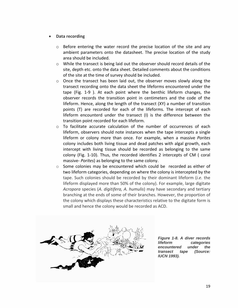
Data recording  

o Before  entering  the water  record  the  precise  location  of  the  site  and  any ambient parameters onto  the datasheet. The precise  location of  the  study area should be included.  

o While the transect is being laid out the observer should record details of the site, depth etc. onto the data sheet. Detailed comments about the conditions of the site at the time of survey should be included. 

o Once  the  transect has been  laid out,  the observer moves  slowly  along  the transect recording onto the data sheet the  lifeforms encountered under the tape  (Fig.  1‐9  ).  At  each  point  where  the  benthic  lifeform  changes,  the observer  records  the  transition  point  in  centimeters  and  the  code  of  the lifeform. Hence, along the length of the transect (XY) a number of transition points  (T)  are  recorded  for  each  of  the  lifeforms.  The  intercept  of  each lifeform  encounterd  under  the  transect  (I)  is  the  difference  between  the transition point recorded for each lifeform.  

o To  facilitate  accurate  calculation  of  the  number  of  occurrences  of  each lifeform, observers should note  instances when the tape  intercepts a single lifeform  or  colony more  than  once.  For  example, when  a massive  Porites colony  includes both  living tissue and dead patches with algal growth, each intercept with  living  tissue  should  be  recorded  as  belonging  to  the  same colony  (Fig.  1‐10).  Thus,  the  recorded  identifies  2  intercepts of CM  (  coral massive‐ Porites) as belonging to the same colony.  

o Some  colonies may be encountered which  could be    recorded as either of two lifeform categories, depending on where the colony is intercepted by the tape. Such colonies should be  recorded by  their dominant  lifeform  (i.e.  the lifeform displayed more than 50% of the colony). For example, large digitate Acropora species (A. digitifera, A. humulis) may have secondary and tertiary branching at the ends of some of their branches. However, the proportion of the colony which displays these characteristics relative to the digitate form is small and hence the colony would be recorded as ACD.  

Figure 1-8. A diver records lifeform categories encountered under the transect tape (Source: IUCN 1993).

  

20  

                      

Figure 1‐9. Schematic diagram of a transect (XY) showing the transition points (T)  for  each  lifeform  crossed  by  the  transect.    The  difference  between  the consecutive  transition  points  is  the  intercept  of  the  lifeform  (Source:  IUCN 1993).     

     

Figure  1‐10.  Diagram showing a transect crossing a  single  colony more  than once. 

       

o More specific taxonomic identification may be included in addition to the life form category, dependent on the observer’s knowledge.  

o It must be emphasized that the lifeform categories specified are the minimum requirements for a regional database. If there is a need to add new categories for specific purposes, the category must allow retrieval of the minimum information (i.e. the new list of categories can readily be collapsed into the old one). For example, if the SC (soft corals) group is divided to note the growth form of soft coral, provision must be made to allow the combination of the new categories back into SC for purposes of exchange.  

  

21  

Standardization 

o Observers must be as consistent as possible when recording the types of colonies, they should collect data at all sites and, where possible, during repeat surveys. 

o Regular training and discussion of lifeforms should be undertaken in the field to ensure that interpretation of lifeform categories is the same for all observers, and that it does not change over time (i.e. data are comparable). 

o The minimum requirements must always be met to ensure that data exchange is possible. 

Data Analysis  

o Relatively large amounts of data will be collected, therefore adequate space for data storage and manipulation must be available.  

o Summary data showing percent cover and number of occurrence of each lifeform may be calculated using the line intercept data. After calculating the intercept from the transition points recorded along the transect, the percent cover of a lifeform category is calculated. 

       Total length of category 

Percent cover = ‐‐‐‐‐‐‐‐‐‐‐‐‐‐‐‐‐‐‐‐‐‐‐‐‐‐‐‐‐‐‐‐‐‐‐‐‐‐‐‐‐‐ x 100                  Length of transect (Y)  

Hence, for Fig. 1‐7,                       I 1+ I 3+ I 5 + I 7     Percent cover lifeform 1 =  ‐‐‐‐‐‐‐‐‐‐‐‐‐‐‐‐‐‐‐‐‐‐‐‐‐ X 100                        Y                           I 2+ I 4+ I 6     Percent cover lifeform 2 = ‐‐‐‐‐‐‐‐‐‐‐‐‐‐‐‐‐‐‐‐‐‐‐‐ X 100                       Y  

o Preliminary calculations of percentage cover and number of occurrences can also be made from the data collected using the Lifeform program. 

o These analyses will provide quantitative information on the community structure of the sample sites. Successive samples can also be compared when the sites have been sampled repeatedly over time.  

o If reefs have been selected to represent both disturbed and pristine sites, then comparison of change detected in these sites may allow recognition of change due to disturbance from natural and man‐induced pressures. This provides a predictive tool in reef management. 

o Where rigorous statistical comparisons of reef community structures within and between sites are needed, greater replication of transects at each 

  

22  

sampling site will be required. This should be identified in a pilot study, but will be at least 8‐10 transects. 

 

Advantages 

o The lifeform categories allow the collection of useful information by persons with limited experience in the identification of coral reef benthic communities. 

o LIT is a reliable and efficient sampling method for obtaining quantitative percent cover data. 

o LIT can provide detailed information on spatial pattern. o If LIT is repeated through time with sufficient replication (see Chapter 7) it 

can provide information on temporal change. Meaningful temporal data requires regular comparisons between observers to overcome observer differences. 

o LIT requires little equipment and is relatively simple.  

Disadvantages 

o It is difficult to standardize some of the lifeform categories. o Objectives are limited to questions concerning percent cover data or relative 

abundance. o It is inappropriate for assessing demographic questions concerning growth, 

recruitment, or mortality. If the objectives of a study specifically address these questions, then photo‐quadrat techniques should be used in addition to LIT. 

o While the LIT can provide detailed  information on spatial pattern,  it cannot provide precise information on temporal change. Therefore, if the objectives specifically address demographic questions or detailed information regarding temporal change  in the benthic community  is required  (i.e.  impact studies), then  belt  transects  and/or  photo‐quadrat  techniques  should  be  used  in addition to LIT. 

 C. Photo-Transect Method

The  video  transect  technique  (Osborne  and  Oxley  1997,  Page  et.  Al.  2001) reduces  the bottom  time of  the observer  to as short as 8 minutes per  transect as compared to 45 minutes with LIT. On the other hand, the video transect technique incurs  high  cost  of  underwater  video  camera  setup  (Php150,000.00)  and  the associated  laboratory  processing  time  to  grab  frames  from  the  videos  to  be analyzed. 

The  Photo‐Transect method  is  a modification  of  the  video  transect  technique described by Osborne and Oxley  (1997).  It  involves  the use of digital  still cameras 

  

23  

attached to a distance bar. A digital camera inside a waterproof case is attached to an  aluminum  distance  bar,  the  length  of  which  is  predetermined  so  that  the substrate covered by the image is 0.5m wide (Fig. 1‐11 & Fig. 1‐12). Photographs of the substrate are taken at 1m intervals to come up with 51 frames per 50m transect. As with  the video  transect  technique,  the digital  images are analyzed using  the 5‐point method (English et al. 1997). 

The photo transect method  is proposed over other survey methods because of several advantages, such as: 

 1) equipment outlay is much cheaper and laboratory processing time is reduced in comparison to the video transect technique; 

 2) the survey can be conducted by non‐technical persons (with little knowledge of advanced technology and even non‐biologists); 

 3) diver bottom time is reduced in comparison to the LIT, and 

 4) taxonomic  identification of biota  is  improved since  image resolution  is much better  than  video  camera  resolution  (0.3  megapixel  vs.  10  megapixel  or higher).  

 

Image and data processing protocols such as color correction, image overlay and considerations on camera selection have been presented by Vergara and Licuanan (2007). The photo  transect  technique  can be promoted as an alternative  low‐cost and non‐technical method to survey coral communities. 

 

 

Figure 1-11. a) Photo showing how the photo transect technique is conducted, b) sample digital output showing the 5-point image overlay used as guide for scoring the image. (Source: Vergara and Licuanan 2007)

  

24  

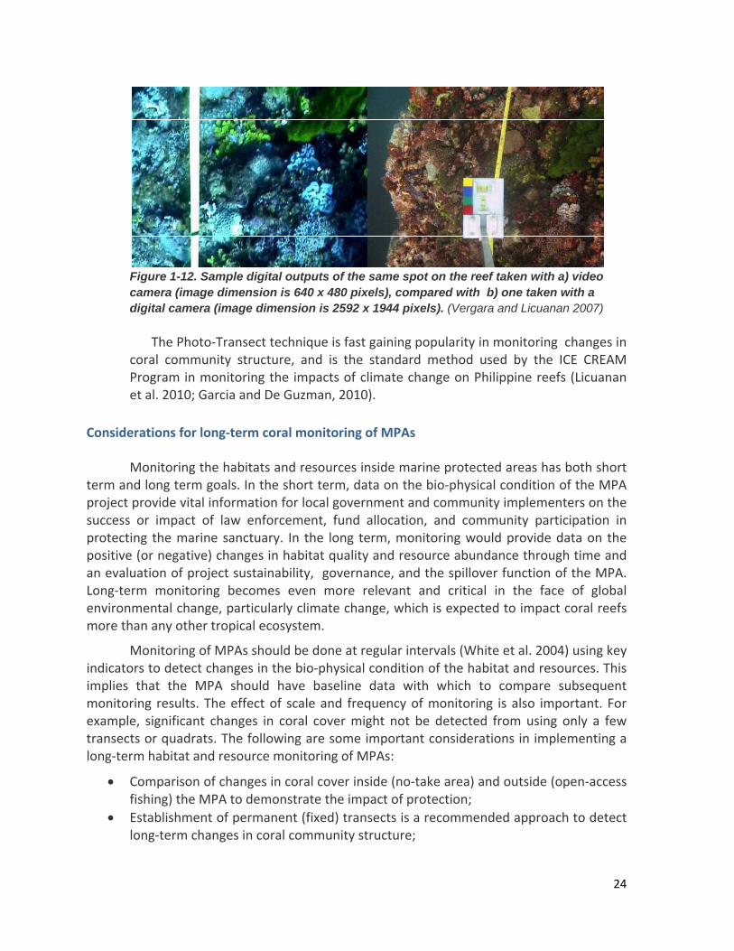
Figure 1-12. Sample digital outputs of the same spot on the reef taken with a) video camera (image dimension is 640 x 480 pixels), compared with b) one taken with a digital camera (image dimension is 2592 x 1944 pixels). (Vergara and Licuanan 2007)

The Photo‐Transect technique is fast gaining popularity in monitoring  changes in coral  community  structure,  and  is  the  standard method  used  by  the  ICE  CREAM Program  in monitoring the  impacts of climate change on Philippine reefs (Licuanan et al. 2010; Garcia and De Guzman, 2010).   

 

Considerations for long‐term coral monitoring of MPAs  

  Monitoring the habitats and resources inside marine protected areas has both short term and long term goals. In the short term, data on the bio‐physical condition of the MPA project provide vital information for local government and community implementers on the success  or  impact  of  law  enforcement,  fund  allocation,  and  community  participation  in protecting  the marine sanctuary.  In  the  long  term, monitoring would provide data on  the positive (or negative) changes in habitat quality and resource abundance through time and an evaluation of project sustainability,  governance, and the spillover function of the MPA. Long‐term  monitoring  becomes  even  more  relevant  and  critical  in  the  face  of  global environmental change, particularly climate change, which is expected to impact coral reefs more than any other tropical ecosystem.  

  Monitoring of MPAs should be done at regular intervals (White et al. 2004) using key indicators to detect changes in the bio‐physical condition of the habitat and resources. This implies  that  the  MPA  should  have  baseline  data  with  which  to  compare  subsequent monitoring  results. The effect of scale and  frequency of monitoring  is also  important. For example,  significant  changes  in  coral  cover might not be detected  from using only a  few transects or quadrats. The following are some  important considerations  in  implementing a long‐term habitat and resource monitoring of MPAs: 

Comparison of changes in coral cover inside (no‐take area) and outside (open‐access fishing) the MPA to demonstrate the impact of protection; 

Establishment of permanent (fixed) transects is a recommended approach to detect long‐term changes in coral community structure;  

  

25  

o Transect location can be fixed by deploying concrete blocks on the reef along which the transect line will be established upon assessment; 

o Location of the monitoring site shall be fixed by getting GPS coordinates;  o Depth of permanent transect locations is preferably shallow (8‐10m) for easy 

monitoring;   

The  number  of  transects  to  deploy  in  both No‐Take  and  Fishing  zones  should  be sufficient to detect significant changes (e.g. the ICE CREAM program deploys at least five (5) 50‐m transects in each site (Licuanan, pers.comm.);  

Where possible, identification of coral species should be made to indicate changes in coral diversity through time; and 

Employing the Photo‐Transect technique  is highly recommended for  long‐term reef monitoring.  

In  addition  to  biophysical  monitoring,  a  regular  evaluation  of  management performance of the MPA should be conducted based on key indicators. Certain instruments to do this are already available, such as the MPA Report Guide (adopted from CRMP 2001) available  with  the  Coastal  Conservation  and  Education  Foundation,  Inc.  (Email:  ccef‐mpa@mozcom.com or at website www.coast.ph).  

Monitoring impacts of climate change and other environmental events

Climate change largely induced by global warming is upon us. Long‐term data show an unprecedented rise in average global temperature and carbon dioxide concentrations in the  atmosphere  in  the  last  four  decades  (Fig.  1‐13).  Coral  reefs  are  constantly  under pressure  from  human‐induced  environmental  changes,    overfishing,  and  other unsustainable  resource uses. Apart  from  these,  reefs now  face  the  impending  impacts of climate  change  that  could    increase  frequency  and  severity  of  natural  hazards  (storms, landfalls, flooding, coastal erosion), sea  level rise,   and  increasing sea temperature (Fig. 1‐14).  

 

 

Figure 1‐13. Rising trend in 

average global temperature 

shows very good correspondence 

with CO2 concentrations. Climate 

experts say the increase in the 

last few decades has never been 

experienced by Earth.  

  

26  

  

Experts also predict increasing risk of the Philippines to more frequent and severe El 

Niño and La Niña events resulting  in droughts and  floods  from more  intense precipitation 

events (Fig. 1‐15).   Coral bleaching and emergence of diseases as a result of warming seas 

can hasten biodiversity loss, reduce fisheries production, and threaten the sustainability of 

coastal livelihoods such as coastal tourism. 

  Recent evidence also suggests that climate change, by  increasing sea temperatures and ocean acidity, may worsen the plight of coral reefs. This has serious consequences for tens  of millions  of  people  and  billion‐dollar  fishing  and  tourism  industries  (CRTR  2008).   When  corals  get  too  warm,  the  symbiosis  with  brown  plant‐like  organisms  known  as zooxanthellae breaks down, and results in coral bleaching.  

  

Figure 1‐15. Correlation between 

climate data shows that the 

Philippines, especially Mindanao 

(higher values in red),  is vulnerable 

to more frequent  El Nino‐La Nina 

(or ENSO) cycles. (Source: Villanoy, 

et al. 2010) 

Fig.  1‐14.  Analysis  of  109‐year 

data on sea surface temperature 

of  Philippine  seas  shows 

increasing    trend  in  SST  despite 

interdecadal  fluctuations 

(Source:  Penaflor  and  David, 

2010).    

 

 

worldmassknowrecenRedaecosyNasuotheroutbr(Plate

durinbegin('hotsdata. 

greatbleac

Coral Blea

Mass  cord’s reefs sinsive bleachinwn  corals  inntly  closed ng),  saying ystems  timegbu, as wellr  Philippine reaks of Croe 1‐5) of Ma

 Massive 

ng  the 1997‐nning  early spots') obse Coral comm

Fig. 1‐16.(Source: R 

The Greatest  threat  tching.   Mass

aching and C

ral bleachingnce the 1980ng  in the Co  the world portions  of they  woul

e  to  heal.  In as off the creefs  are  liwn‐of‐Thornsinloc, Zamb

bleaching  w‐98 El Nino June  untilrved in the munities suff

 World‐wideReefBase 19

t Barrier Reto  the Greas  coral bleac

Climate cha

g  caused by0s (Fig. 1‐16)oral Triangle(WWF  201world‐famod  be  off  lin  the  Philipcoast of the wikely  to  havns seastars.bales were r

was  also  obevent.   Arcl  late  Novecountry durfered signific

e  occurrenc997). 

eef Marine Pat  Barrier  Reching events

ange 

y global wa).  The moste, a vast ma0  – www.wous  dive  stiemits  until  Opines,  bleacwestern muve  been  affeRecent incidreported (De

bserved  in  mceo, et al.  (2ember  1998ring this samcant decreas

ces  of coral 

Park Authoreef,  causings due  to ele

rming  is  thrt recent El Narine regionwwf.org.ph).es  (e.g.  tropOctober  to ching  has  bnicipality ofected  as wedents of bleaeocadez/ICE 

many  reefs 2001)  repor8,  coincidinme period shse in live cor

bleaching f

rity  considerg  ocean warevated ocea

reatening  thNiño (2009‐2n that  is homThe Malayspical  islandsgive  the  freen  reportef Taytay, Palaell,  exacerbaaching in theCREAM, Ma

throughoutted  that bleng  with  theown by sateral cover of u

from 1969 to

rs  climate  crming whichan  temperat

he health o2010) has came to 76% osian  governs  of  Tiomanragile  coral ed  in  Anilaoawan. Numeated  by  locae Philippine ay 2010).  

t  the  Philipeaching occuermal  anomellite‐derivedup to 46%. 

 o 1996     

hange  to beh  increases tures occurr

 

27 

of  the aused of all ment n  and reef 

o  and erous alized reefs 

pines urred malies d SST 

 

e  the coral ed  in 

  

28  

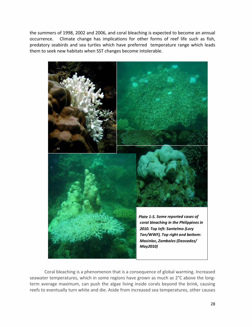
the summers of 1998, 2002 and 2006, and coral bleaching is expected to become an annual occurrence.      Climate  change  has  implications  for  other  forms  of  reef  life  such  as  fish,  predatory  seabirds and  sea  turtles which have preferred    temperature  range which  leads them to seek new habitats when SST changes become intolerable.   

  Coral bleaching is a phenomenon that is a consequence of global warming. Increased 

seawater temperatures, which in some regions have grown as much as 2°C above the long‐term average maximum, can push  the algae  living  inside corals beyond  the brink, causing reefs to eventually turn white and die. Aside from increased sea temperatures, other causes 

Plate 12. Some reported cases of 

coral bleaching in the Philippines in 

2010. Top left: Santelmo (Lory 

Tan/WWF), Top right and bottom: 

Masinloc, Zambales (Deocadez/ 

May2010)  

Plate 1‐5.

  

29  

of stress  include disease, pollution, sedimentation, cyanide fishing, changes  in salinity, and storms.  Since  March  this  year,  about  50  different  organizations  and  individuals  have reported  signs  of  coral  bleaching  in  the  Coral  Triangle  region. Up  to  100%  bleaching  on susceptible coral species have been reported, and in some areas, severe bleaching has also affected the more resistant species. 

  With many  areas  showing  signs  of mass  bleaching,  it  has  become  apparent  that 

more weight  needs  to  be  put  behind  long‐term  conservation  strategies,  such  as marine protected area management, preventing coastal and marine pollution, as well as promoting sustainable  fisheries.  Richard  Leck,  Climate  Change  Strategy  Leader  of  the  WWF  Coral Triangle Programme, declared that this widespread bleaching is alarming because it directly affects  the health of our oceans and  their ability  to nurture  fish  stocks and other marine resources on which millions of people depend  for  food and  income. Leck   suggested  that “well‐designed and appropriately‐managed networks of marine protected areas and locally managed marine  areas  are  essential  to  enhance  resilience  against  climate  change,  and prevent further loss of biodiversity, including fisheries collapse”  Coral Diseases Despite  their  importance coral  reefs continue  to be  impacted by human activities, climate  change,  land  and  marine‐based  pollution,  habitat  degradation  and  overfishing. Many of these impacts have obvious and immediate effects often leading to mass  mortality of corals. Some effects, however, such as those from chemical pollutants, wastes or excess nutrients are more insidious, and their impacts may be difficult to understand and quantify. One  phenomenon  which  has  recently  gained  the  attention  of  coral  reef  scientists  and managers is the increased incidence in coral disease. Diseases affecting corals particularly in the Caribbean  reefs, have  increased  in both  frequency  and  severity within  the  last  three decades (Raymundo and Harvell 2008).  

 What is a coral disease? 

Diseases are a natural aspect of populations –  they are one mechanism by which population numbers are kept  in check. Disease  involves an  interaction between a host, an agent, and the environment. Infectious biotic diseases are caused by microbial agents, such as bacterium, fungus, virus, or protest that can be spread between hosts and organisms and negatively  impact  the hosts’ health  (Raymundo and Harvell 2008). Other  forms of disease that may  have  impacted  corals may  be  considered  abiotic  diseases;  they  do  not  involve microbial agents but impair health, nonetheless. Environmental agents such as temperature stress,  sedimentation,  toxic  chemicals,  nutrient  imbalance  and  UV  radiation  are  such examples.  In  addition,  noninfectious  diseases  are  not  transmitted  between  organisms, though  they may be  caused by a microbial agent.  For example,  certain microbes  secrete toxins  released  by  the  bacterium  Clostridium  botulinum  cause  a  non‐infectious  but deleterious disease in organisms that consume it.  

  

30  

Research on coral diseases  is an emerging  field  in marine  science. Pioneers  in  the field  have  identified    five  coral  diseases  for which  Koch’s  postulates  have  been  fulfilled showing disease, host coral and microbial pathogen (Fig. 1‐17). The classic way to prove a microorganism  cause  disease  is  to  satisfy  Koch’s  postulate.  A  microorganism  must  be isolated from a diseased individual. That “isolate” is then used to infect a healthy individual. The  same disease must develop, and  the  same organism must be  isolated  from  the new infection.  This  classic  method  is  a  tough  challenge  in  the  face  of  unculturable  marine microorganisms and polymicrobial syndromes, requiring molecular approaches. 

 

Fig. 1-17. Five most  common  groups  of  coral  diseases  (Source:  Raymundo  and  Harvell 2008).

Carribean sea fan Gorgonia ventalina with multiple aspergillotic lesions. Photo. E. Weil

 

Environmental stress and Coral Disease 

  An understanding of the influence that the environment plays in disease outbreaks 

could guide the development of useful management strategies (Fig. 1‐18).   

  

31  

 

Fig. 1‐18. Relationship between host and disease agent in corals (Source: Raymundo and 

Harvell 2008). 

 

As with most aspects of management of infectious disease in a marine setting, it is a work in progress and it is critical to keep in mind that all infectious syndromes are different and may  respond  in  different  ways  to  environmental  change.  However,  identifying  the factors  that  control  the  most  important  infectious  syndromes  is  a  key  management strategy. Morbidity or mortality  in  corals  can be  caused by  tissue  loss  from predation or disease (Fig. 1‐19 to Fig. 1‐20).    

  

32  

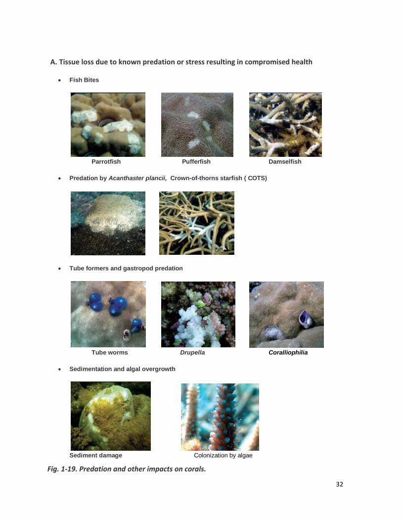
 A. Tissue loss due to known predation or stress resulting in compromised health 

   

Fig. 1‐19. Predation and other impacts on corals.  

Fish Bites

Parrotfish Pufferfish Damselfish

Predation by Acanthaster plancii, Crown-of-thorns starfish ( COTS)

Tube formers and gastropod predation

Tube worms Drupella Coralliophilia

Sedimentation and algal overgrowth

Sediment damage Colonization by algae

  

33  

B. Tissue loss due to biotic and abiotic diseases  

This refers to lesions that do not have any of the discrete patterns of tissue loss or skeletal damage consistent with predation or compromised health states described above. 

C. Tissue loss: within distinct bands  

 D. Tissue discoloration  

 

  

E. Growth anomalies (Skeletal deformations) 

Black band disease (a&b) Skeletal eroding band Brown band

Ulcerative white spots White syndrome Atramentous necrosis

Pigmentation response Trematodiasis Unusual bleaching patterns

Galls Growth anomalies of unknown causes

  

34  

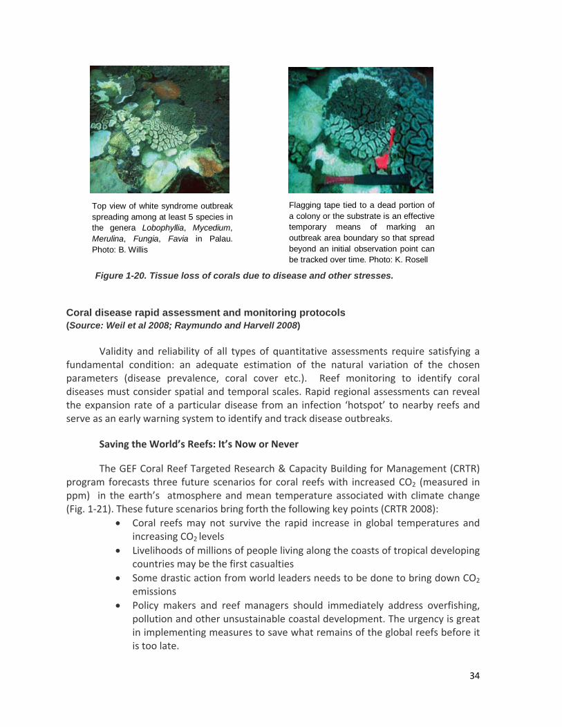
Figure 1-20. Tissue loss of corals due to disease and other stresses.

Coral disease rapid assessment and monitoring protocols (Source: Weil et al 2008; Raymundo and Harvell 2008)

Validity and  reliability of all  types of quantitative assessments  require  satisfying a fundamental  condition:  an  adequate  estimation  of  the  natural  variation  of  the  chosen parameters  (disease  prevalence,  coral  cover  etc.).    Reef  monitoring  to  identify  coral diseases must consider spatial and temporal scales. Rapid regional assessments can reveal the expansion rate of a particular disease  from an  infection  ‘hotspot’  to nearby reefs and serve as an early warning system to identify and track disease outbreaks. 

Saving the World’s Reefs: It’s Now or Never 

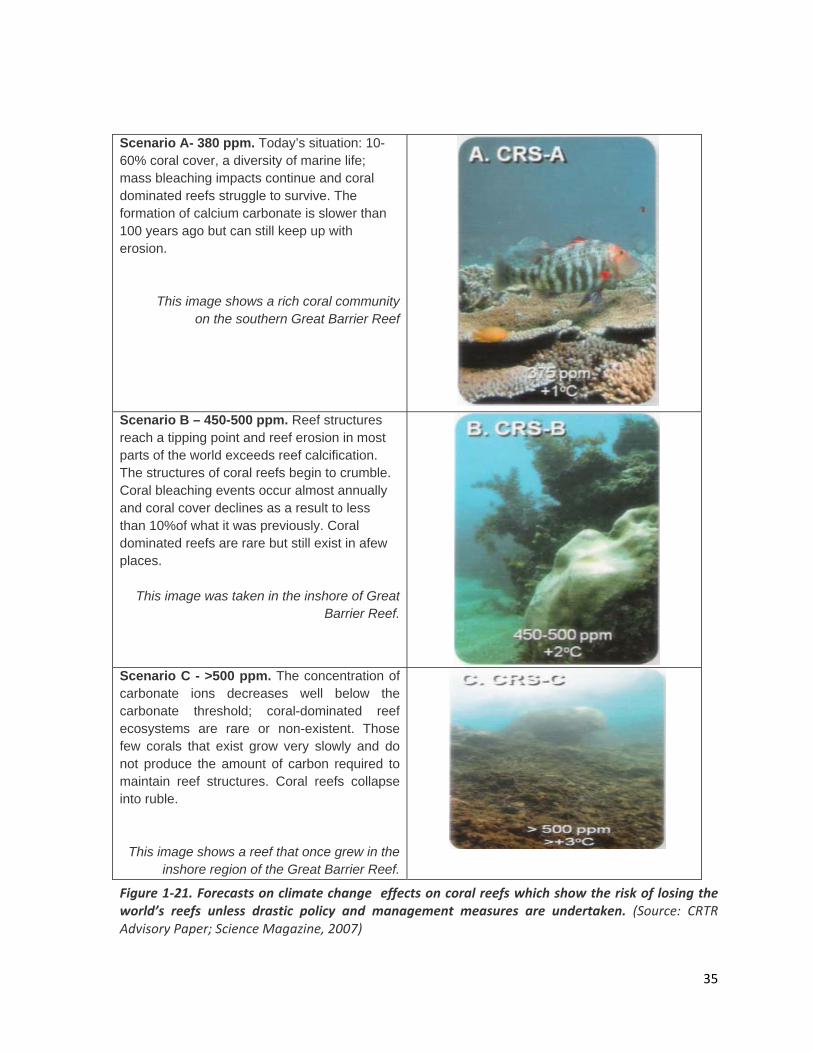
The GEF Coral Reef Targeted Research & Capacity Building for Management (CRTR) program  forecasts  three  future  scenarios  for coral  reefs with  increased CO2  (measured  in ppm)    in  the earth’s   atmosphere and mean  temperature associated with climate change (Fig. 1‐21). These future scenarios bring forth the following key points (CRTR 2008): 

Coral  reefs may not  survive  the  rapid  increase  in  global  temperatures  and increasing CO2 levels 

Livelihoods of millions of people living along the coasts of tropical developing countries may be the first casualties 

Some drastic action from world leaders needs to be done to bring down CO2 emissions 

Policy makers  and  reef managers  should  immediately  address  overfishing, pollution and other unsustainable coastal development. The urgency is great in implementing measures to save what remains of the global reefs before it is too late.  

Top view of white syndrome outbreak spreading among at least 5 species in the genera Lobophyllia, Mycedium, Merulina, Fungia, Favia in Palau. Photo: B. Willis

Flagging tape tied to a dead portion of a colony or the substrate is an effective temporary means of marking an outbreak area boundary so that spread beyond an initial observation point can be tracked over time. Photo: K. Rosell

  

35  

  

Scenario A- 380 ppm. Today’s situation: 10-60% coral cover, a diversity of marine life; mass bleaching impacts continue and coral dominated reefs struggle to survive. The formation of calcium carbonate is slower than 100 years ago but can still keep up with erosion.

This image shows a rich coral communityon the southern Great Barrier Reef

              Scenario B – 450-500 ppm. Reef structures reach a tipping point and reef erosion in most parts of the world exceeds reef calcification. The structures of coral reefs begin to crumble. Coral bleaching events occur almost annually and coral cover declines as a result to less than 10%of what it was previously. Coral dominated reefs are rare but still exist in afew places.

This image was taken in the inshore of Great Barrier Reef.

           Scenario C - >500 ppm. The concentration of carbonate ions decreases well below the carbonate threshold; coral-dominated reef ecosystems are rare or non-existent. Those few corals that exist grow very slowly and do not produce the amount of carbon required to maintain reef structures. Coral reefs collapse into ruble.

This image shows a reef that once grew in the inshore region of the Great Barrier Reef.

  

Figure 1‐21. Forecasts on climate change   effects on coral reefs which show the risk of  losing the world’s  reefs  unless  drastic  policy  and management measures  are  undertaken.  (Source:  CRTR Advisory Paper; Science Magazine, 2007) 

  

36  

Drawing up a Monitoring Plan

One important consideration in reef monitoring is we cannot observe all things at the same time.    There  is  an  urgent    need  to  draw  up  a monitoring  plan  for  the  long‐term  observation  of changes on the reef ecosystem (Fig. 1‐22). Community participation is also essential; complementing the indigenous knowledge of fishers with scientific knowledge and information from monitoring can give us a very representative picture of what is happening. 

Figure  1‐22.  Some  monitoring  activities  that  can  be  conducted  to  compare  benthos,  fish, invertebrates and vegetation inside and outside MPAs. (Source: Uychiaoco et al. 2010).  

 

 

For example, you could monitor coral, fish, invertebrates and algae, inside and outside an MPA.

  

37  

 

 

Trainer’s Tips:

Below are some useful tips from Uychiaoco et al. 2010: 1. Be clear about what you want to know, then select a few things to observe in several 

places through time.  2. Observe the things of interest that are likely to change due to poor or good 

management. 3. Observe in different kinds of places: inside and outside the management zone or use 

zone (e.g. inside and outside the marine protected area (MPA)). Try to observe at 5 stations within each management zone. 

4. Observe before, and every year after establishment of the management actions, during each season. Things that don’t change much can be observed less frequently. 

5. Monitor every year: during the dry season, the northeast monsoon and the southwest monsoon...so that changes from season to season can be noted. (Corals may be monitored only once a year since they change very slowly). 

6. You could monitor algae, fish, and invertebrates inside and outside an MPA. 7. It is important to note what factors may cause the decrease (‐) or increase (+) in 

certain parameters, such as coral cover, fish abundance, algal growth, etc.   

 

 

 

 

Fi(Kuiter awaters) halso  linkaquarium2005).  

 Fconductebe  caughenvironmto attainto the enthe  currerelegatedand reso

Timportanmanage Philippinor  AFMAsectors developmmanagemthe fishe

Reef Fis

Cand  comthe coralCoral reeeconomithe mostsupplyinglargely  rrapid  deSoutheas 

M

ishes  are  thnd Debeliushave the higed  to  the  cm fish and ac

Fish  populated by MSU Nht  by more mental probl a more susnvironmentaent  economd to some durces are all

he sustainabnt  law, the Pand conserves 1998), alA,  was  pass(Congress  oment becausment of resories sector (

h Diversity

oral  reef  fismplex  colorsl reefs, thus ef fish are imes as sourcet popular ecg  the  globaesponsible ecline  in  biost Asian reef

MONITORI

he  most  wis 2006). Coaghest fisherycoastal  areaccounts for 3

tions  can  beNaawan (199efficient  fislems of the stainable foral problems mic  crisis  endegree as nalocated to m

ble developmPhilippine Five  the  fisheso the Agricsed  to  revivof  the  Philise they explources as a mIsrael and Ro

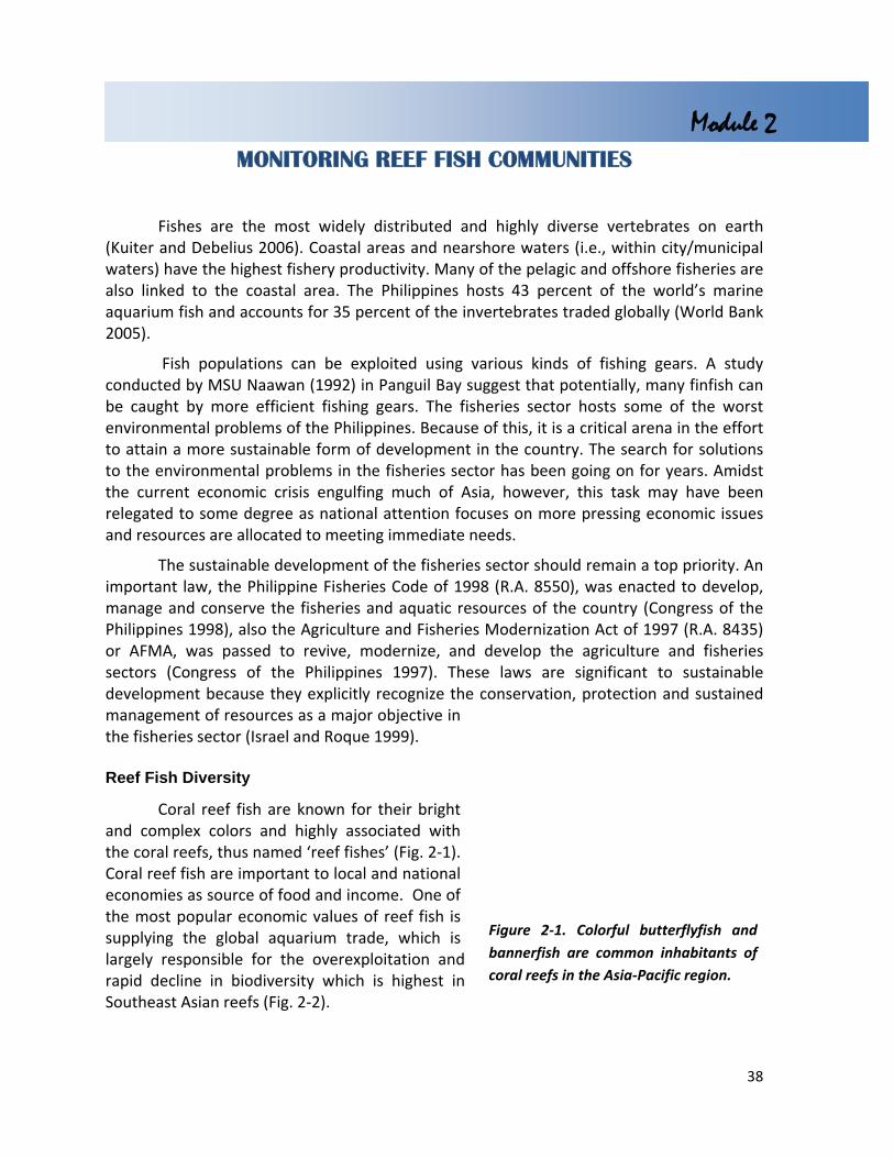
sh are knows  and  highlynamed ‘ree

mportant to e of food andconomic valal  aquariumfor  the  oveodiversity  wfs (Fig. 2‐2).  

ING REEF

dely  distribastal areas ay productivity.  The  Philip35 percent o

e  exploited 92) in Pangushing  gears.Philippines. rm of develoin the fishegulfing mucational attenmeeting imm

ment of the sheries Codries and aquculture and ve,  modernippines  199licitly recognmajor objectoque 1999).

wn  for  their y  associatedf fishes’ (Figlocal and nad income.  Oues of reef 

m  trade,  wherexploitatiohich  is  high 

F FISH C

buted  and  hnd nearshoy. Many of tppines  hostsof the invert

using  variouil Bay sugge  The  fisheriBecause of opment  in teries sector hch  of  Asia, ntion focusemediate need

fisheries sece of 1998 (Ruatic resourFisheries Moize,  and  de97).  These  lnize the contive in  

bright d  with g. 2‐1). ational One of fish  is hich  is on  and hest  in 

Fig

ba

co

COMMUNI

highly  diversre waters (i.the pelagic as  43  percentebrates trad

ous  kinds  oest that poteies  sector  hthis, it is a che country. has been gohowever,  ths on more pds. 

ctor should R.A. 8550), wrces of  the codernizationvelop  the  alaws  are  sinservation, p

gure  2‐1.  C

annerfish  are

oral reefs in th

ITIES

se  vertebrat.e., within cand offshoret  of  the woded globally

f  fishing  geentially, manhosts  some critical arenaThe search 

oing on for yhis  task mapressing eco

remain a towas enactedcountry  (Conn Act of 199agriculture  agnificant  toprotection a

Colorful  butte

e  common  in

he Asia‐Pacif

3

Module

tes  on  eartity/municipae fisheries arorld’s mariny (World Ban

ears.  A  studny finfish caof  the worsa in the effofor solutionyears. Amidsy  have  beeonomic  issue

p priority. Ad to developngress of  th7 (R.A. 8435and  fisherieo  sustainabland sustaine

erflyfish  and

nhabitants  of

fic region.    

 

38 

e 2

th al re ne nk 

dy an st rt ns st en es 

An p, he 5) es le ed 

d 

f 

  

39  

 

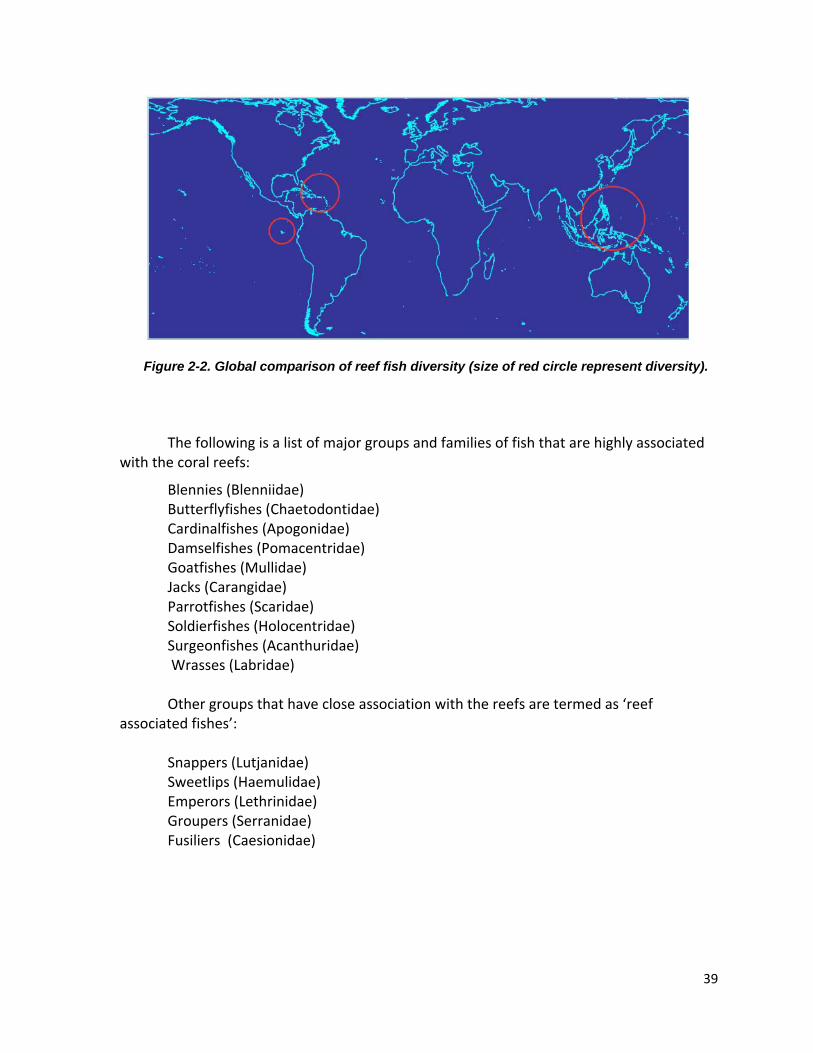
Figure 2-2. Global comparison of reef fish diversity (size of red circle represent diversity).

  

The following is a list of major groups and families of fish that are highly associated with the coral reefs: 

Blennies (Blenniidae) Butterflyfishes (Chaetodontidae)  Cardinalfishes (Apogonidae)  Damselfishes (Pomacentridae) Goatfishes (Mullidae) Jacks (Carangidae) Parrotfishes (Scaridae) Soldierfishes (Holocentridae) Surgeonfishes (Acanthuridae)  Wrasses (Labridae) 

 Other groups that have close association with the reefs are termed as ‘reef 

associated fishes’:   

Snappers (Lutjanidae) Sweetlips (Haemulidae) Emperors (Lethrinidae) Groupers (Serranidae) Fusiliers  (Caesionidae) 

     

  

40  

Characteristics of coral reef fish  

Coral reef fish are   highly diverse; up to 4,000 species are found  in the  Indo‐Pacific region (18% of all living fishes). About 2,500 species are found in the Philippines, touted as  the  Center  of  the  Center  of  reef  fish  diversity (Carpenter  and  Springer  2005).  They  occur  in many  forms and  sizes –  some  fish as  tiny as   3 cm SL (Minilabrus striatus), others as big as  the Napoleon wrasse Cheilinus undulatus which can reach 290 cm SL.  

 Reef  fish  have  highly  specialize  feeding 

structures used as basis for functional groupings as  grazers  (scarids  or  parrotfish),  invertebrate feeders  (labrids  or  wrasses),  piscivores (groupers,  cardinal  fish,  lizardfish),  planktivores (fusiliers, many damselfish).  

 Ecological & economic importance 

  Coral  reef  fish play an  important ecological  role  in  the marine ecosystem,  such as maintenance  of  complex  trophic       structure,  standing  stock  to  support fisheries  and  biodiversity,  nutrient recycling, and  reef habitat modification.  

They are also  important as high‐value  food  source,  and  their  colorful variety  and  aesthetic  value  feed  the world  aquarium  trade  and  attract  a multi‐million  dollar  tourism  industry  in many countries in Asia‐Pacific. 

Status of Philippine Reef Fishes 

  Figure 2‐3 presents the profile on fish biomass across seven biogeographic zones  of  the  Philippines  based  on biomass  estimates.  On  a  scale  of  very low  (red)  to  very  high  biomass  (dark blue),  the  figure  shows  that  most Philippine reefs currently support  low fish biomass, most possibly  a  consequence of overfishing and habitat degradation.   

 

  Figure 2‐4. Comparison of fish biomass across     

  different biogeographic zones (Nañola 2006).  

Figure  2‐3.  The  Napoleon  wrasse, Cheilinus undulates, is one of the giants of the reef.

  

41  

Methods of Monitoring 

Why monitor fish communities in MPAs?    Monitoring the status of reef fish communities allows management to find out if the 

MPA  project  has  achieved  its  goals,  and  if  positive  impacts  of  protection  are  already observed.  It  is  also  a  means  of  evaluating  management  performance  in  terms  of enforcement of sanctuary rules, particularly the “no take” areas.   

Long‐term monitoring of reef fishes requires the availability of baseline assessment conducted before MPA establishment or during the early years of the project.  Many MPAs, however, do not have the benefit of a baseline assessment  

Assessment or monitoring of reef fish communities in MPAs will gather the following information: 

Species richness 

Biodiversity  

Determine the status of the stocks inside the MPA 

Degree of overexploitation (in areas outside the MPA)  

Determine  the  classification  of  fish  groups,  e.g.  top  carnivores/food  fishes, Indicator of reef health, grazers, etc. 

 

Methods on reef fish assessment 

1. Fishery‐ based survey o Municipal fishery monitoring (i.e. different fishing gears) 

o Catch composition 

o Extraction rate 

o Length‐frequency  analyses  (i.e  FiSAT)  to  obtain  estimates  of  population 

exploitation rate 

Constraints of this method include:   

o Difficulty in getting the total (all or major species) stock 

o Bias brought about by the selectivity of the fishing gears 

Fisheries‐Independent  survey  to  obtain  data  on  fish  diversity,  abundance  and biomass are available, but many of them are destructive, such as blast fishing, use of poison and use of fishing gears. 

 

2. Underwater fish visual census 

Fish visual census (Fig. 2‐5) is a fishery‐independent survey technique that has a number of advantages, as follow: 

o Rapid 

  

42  

o Non‐destructive o Inexpensive o Can be done repeatedly o Gives a snap shot of the fish composition per unit time and area 

 

The FVC technique obtains three types of information: 

Species  diversity  =  listing  of  fish  at  the  species  level  but  limited  within  the 

desired width  of the transect 

Fish density = number of fish per unit area (as area surveyed is known) 

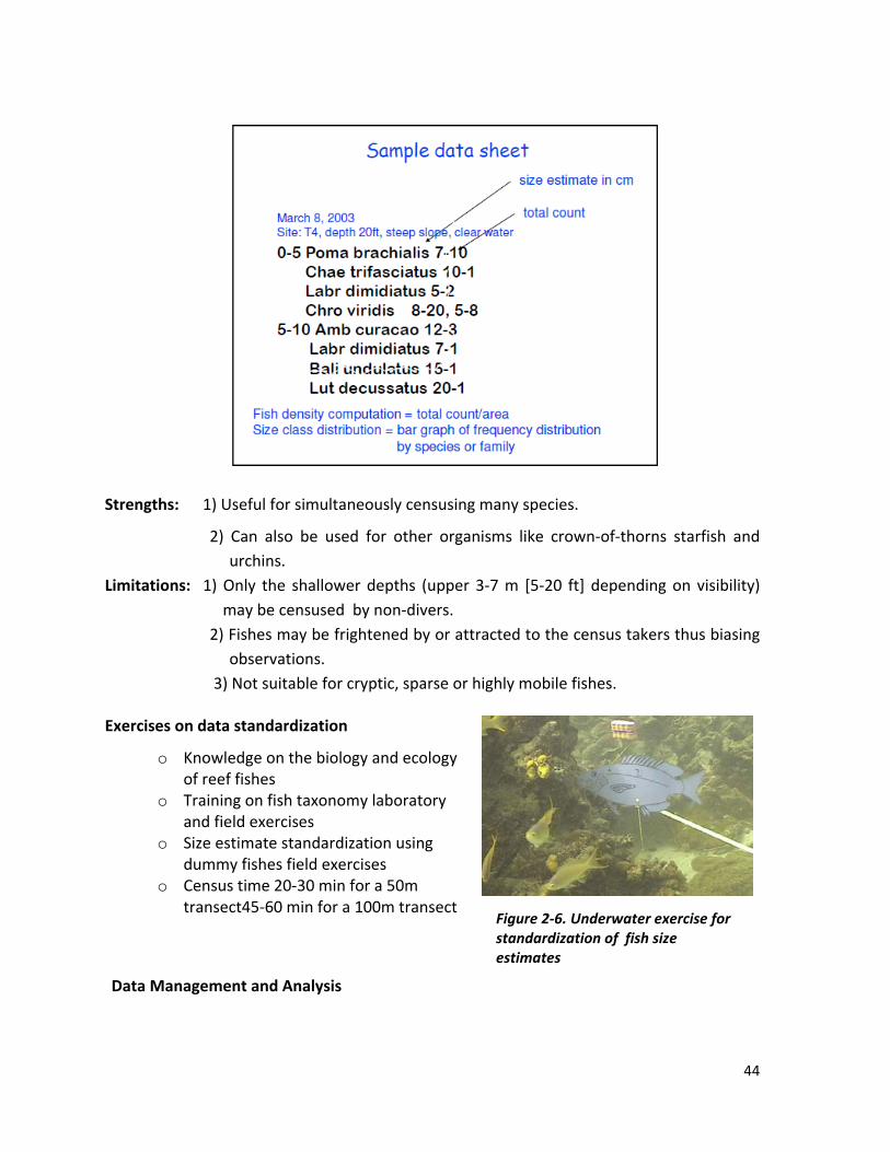
Size class distribution = fish sizes are estimated during the census 

Fish Visual Census (FVC) - identification and counting of fishes observed within a define area. Fish Visual Census can be used to estimate the variety, numbers, and even sizes of common, easily-seen, easily-identified fishes in areas of good visibility. This information may reflect the health of the fish stocks within the surveyed coral reef areas.

Requirements 

Picture Book of the animals (e.g. fishes) to be counted 

Goggles or mask and snorkel 

One or two 50‐m lines each marked every 5 m 

Underwater slate with attached pencil 

 

Optional 

Boat (depending on where the survey site is)  Laminated  fish  identification  guide  (if  observers  are  not  familiar with  the 

various fish types)  Laminated butterflyfish identification guide to (if indicator species are to be 

censused)  Fins  Life jackets 

 

The FVC Procedure  

Figure 3‐5. Underwater fish census requires scuba diving skills but may be done by snorkeling. 

  

43  

1. Select the sampling stations and  fish communities to be censused. 2. Copy the Data Form 5A (Uychiaoco et al. 2010)   onto the slates and draw columns 

for the different size classes. 

3. Lay the transect line on a constant depth contour. Record the depth. 

4. Wait 10‐15 minutes  for  the disturbed  fishes  to  return. Be careful not  to disturbed 

the fishes during census. 

5. Starting at one end of the line, each observer floats on each side of the transect line 

while observing 5‐m to his/her side of the transect and forward until the next 5‐m 

mark. 

6. Both observers swim to and stop every 5‐m along the line to record the count of fish 

per size class until the transect is completed. Generally, the faster moving fishes are 

counted before the slower moving fishes are counted. Each transect covers an area 

of 500m2 (50 m x 10 m width). Obtain the total count on both sides of the transect 

and transcribe onto Data Form 5A. 

7. Classify the group of transect according to your purpose for data summarization. For 

example: 

* reef zones or types (e.g. reef flat, reef slope, fringing reef, offshore reef,  etc.) 

*  time of  sampling  (e.g. year 1/dry season, year 1/wet  season, year 2/dry  season, 

etc.)  

* management or use zones (e.g. sanctuary, fishing grounds), and or 

*intensity of impacts (e.g. high poluution, medium pollution, low pollution) 

List the transect by groups along the upper portion of the Summary Form. 

8. List  the  fish  groups  or  fish  types  (by  groups)  along  the  left  side  of  the  Summary 

Form. 

9. Total the counts of the different size classes for each type of fish per transect. 

10. Write these sub‐totals onto the appropriate boxes on a copy of the summary form. 

11. Sum up sub‐totals for each transect group. 

12. Standardize the sub‐total by sample size; divide the total counts by the number of 

transect actually observed. 

 Example 12+11+5+3+5= 7 Fishes/ transect 

                    5 transect 

13. Choose  a  few  fish  type  of  interest  and  list  these  along  the  left  side  of  the  Fish Graphing Form. 

14. List the zone/sector, month, and year on the designated space on the form. 

15. Use the following guide to represent the average observed in each zone/sector and month/year. 

  

44  

 

Strengths:      1) Useful for simultaneously censusing many species. 

2)  Can  also  be  used  for  other  organisms  like  crown‐of‐thorns  starfish  and 

urchins. 

Limitations:   1) Only  the  shallower depths  (upper 3‐7 m  [5‐20  ft] depending on visibility)  

may be censused  by non‐divers. 

2) Fishes may be frightened by or attracted to the census takers thus biasing 

observations. 

 3) Not suitable for cryptic, sparse or highly mobile fishes.  

Exercises on data standardization 

o Knowledge on the biology and ecology of reef fishes 

o Training on fish taxonomy laboratory and field exercises 

o Size estimate standardization using dummy fishes field exercises 

o Census time 20‐30 min for a 50m transect45‐60 min for a 100m transect 

Data Management and Analysis 

 

Figure 2‐6. Underwater exercise for standardization of  fish size estimates 

  

45  

1. Fish Abundance – obtain mean density (number of fish/m2) per species or family, 

then  add  up  densities  of  all  species;  obtain  relative  abundance  (%)  of  each 

species or family:   RA (%) =  mean density per family/total number of all fishes x 

100 

2. Fish biomass estimate = based on the size estimate and using the relationship of  W=aLb,  weight can be computed, where a and b are growth parameters that are unique to each species (available at www.fishbase.org). 

e.g.  Acanthurus nigricans  a=0.067;  b=2.669 [a and b values from existing length‐weight   (cm‐g)  relationship  

data];   from data recorded:  L=15cm,  total count = 5 

    W= 0.067(152.669)*5 W= 461.352 grams 

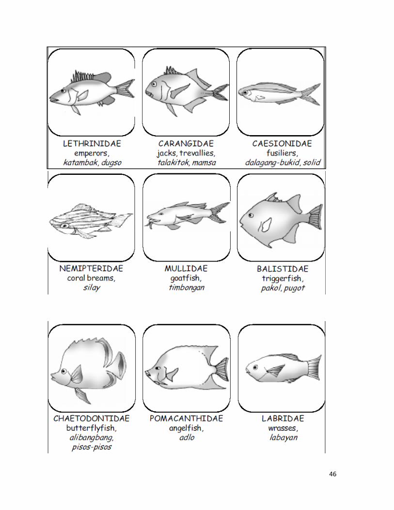
Common Reef Fish Families  

 

Figure  3‐7    show  the  common  fish  families  useful  in  getting  familiar with  the  general 

shape and morphology of various reef fish (reproduced from Uychiaoco et al 2010:) 

  

46  

  

47  

Figure 3-8. Field guides on common fish families with color pictures like the above are very useful. (Source: Nañola et al 2006)

  

48  

Module 3

MONITORING SEAGRASS COMMUNITIES

Seagrasses are  considered as unique,  submerged vascular plants  found  in  shallow  coastal 

areas of the marine environment  (Hemminga and Duarte 2000). Morphologically they compose of 

creeping and erect rhizomes which serve as roots and are also used for attachments as they grow. 

They are the only submerged angiosperm found mostly  in all coastal waters of the world except  in 

the arctic (Den Hartog 1970). 

  Seagrass and seagrass meadows (Fig. 3‐

1) are widely distributed and considered  to be 

among the most productive marine ecosystems 

(Fonseca  and  Calahan  1992;  Agostini  2003). 

About  60  species  of  seagrasses  have  been 

recorded  worldwide  (Den  Hartog  1970;  Kuo 

and McComb  1989),  16  species  of  which  are 

found  in  the  Philippines,  considered  to  be 

among  the  richest  in  the  world  (Fortes  1989 

and Vermaat et al. 1995). 

The  seagrass  ecosystem  provides  enumerable 

environmental  functions;  they  help  reduce 

current  and  wave  energy,  filter  suspended 

sediments  from  water,  and  stabilize  bottom 

sediments  (Fonseca  and  Calahan  1992).  They 

serve as primary producers (and play an important role in the complex food chain), habitat, feeding 

and  spawning  grounds  for  both  juvenile  and  adult  marine  organisms  (invertebrates  and 

vertebrates), including commercially important fish species (Duffy 2006).  

  The  seagrass ecosystem  in  the Southeast Asian  regions  is  threatened by both natural and 

human‐induced disturbances.  In Philippine coastal waters, seagrass  losses are  largely attributed to 

the use of destructive fishing methods, and increasing pollution and siltation (Fortes 1990).     

  Seaweeds  are  macrobenthic  marine  algae  that  forms  a  conspicuous  component  of  the 

primary producers  in  the  shallow marine  environment.  They possess different  types of pigments 

such as chlorophylls, carotenoids, phycobilins, and other accessory pigments which enable them to 

Figure 3‐1. A healthy seagrass meadow is one 

of  most  productive  ecosystems  in    tropical 

coasts.  

  

49  

synthesize organic  compounds  from  simple  compounds  such  as water  and  carbon dioxide  in  the 

presence of light as source of energy.  

 

Monitoring Methods  

Monitoring seagrass communities consider several factors in order to determine changes in community structure and environmental conditions.  Assessment of areal coverage (seagrass cover) can provide a quick assessment of the extent of vegetation, but ocular readings could be very subjective and depend largely on the ability of the person doing the survey.  Shoot density could provide a more accurate data if done properly.  Changes in shoot density would indicate vigor of the vegetation or its ability to reproduce or expand under a given environmental condition. 

To detect changes in habitat condition  with time, a regular monitoring protocol is necessary.  Quarterly monitoring is recommended, but if this is not possible, at least a survey every six months should be done. In every monitoring site,  two permanent transects should be established.  Both ends of the transect should be marked with a post, and the corresponding coordinates taken using the GPS.  Markers should be reinforced later for future monitoring. 

This training module, although technical in nature, can be used to train village people to conduct survey and monitoring of seagrass habitats in their area.  It is a simplified yet robust enough method to generate information to detect changes in the seagrass habitat in terms of seagrass cover, species composition and abundance, flora and faunal associates composition and abundance. 

Materials needed 

o 50m pvc transect tape or calibrated  polyethylene rope (calibrated every 5 m interval) o Mask & snorkel or goggles o Underwater slates with attached pencil o Boat and fuel o Laminated seagrass, invertebrates, and fish identification guides (optional) o Global positioning system (GPS) o Herbaria presser and associated paraphernalia 

Field  assessment procedure 

1. Before  conducting  the  transect  survey,  it  is  important  to  standardize  readings  among observers  or monitors.    This  is  to  ensure  validity  of  data  particularly  on  seagrass  cover.  Values  for cover of  the  same  species  in  the  same area are very subjective and may differ greatly among observers as shown in Table 3‐1 below: 

Table 3‐1.   Example 1. Variable  readings of percent cover of  the  two  seagrass  species by local monitors during the start of the standardization technique. 

  Participants 

Species  A  B  C  D  E  F  G 

Thalassia  20  15  5  20  50  20  10 

Enhalus  50  70  10  60  90  50  40 

  

50  

2. As observed during many training activities, wide ranges of values were generated from the participants from a single quadrat.   For example, participant C gave a very  low score while participant  E  gave  a  relatively  high  score.    After  explaining  the  assumptions  and  some techniques for reading, variability among values can be greatly reduced as shown in Table 3‐2. 

Table 3‐2.  Example 2. Improvement in readings of percent cover by local monitors after the standardization technique. 

  Participants 

  A  B  C  D  E  F  G 

Thalassia  20  10  15  30  20  10  15 

Enhalus  30   40  20  40  40  40  20  

3. If done with careful planning and frequent discussion with the local researchers or monitors, standardization of readings can be achieved. Although values may still vary, it will be within the acceptable range. 

4. Locate  the permanent markers,  and  then  attach  both  ends with  the pre‐calibrated  rope.  The rope should be calibrated every 5 meters with a high visibility tape or string to facilitate survey while swimming over.  

5. Start sampling five meters from the post and at every 5 meters interval until the end of 50 meters.  There shall be a total of ten (10) quadrats for every transect line. 

6. In  the  slates,    write  down  the  date  of  survey,  time,  location,  coordinates  (latitude  & longitude) using the GPS, transect number,  observer’s name, depth and other observations. 

7. At least two observers are needed to conduct the sampling.  In case this is not possible, one person or observer  can do  everything  –  although  this may  take  some  time.    Ideally, one person shall record the percent cover and density for seagrass, and another person shall do the invertebrates and fish count.  It is recommended further that the same person shall do the visual census of fish in both the seagrass and coral transect. 

A. Seagrass and seaweed community structure 

The recommended quadrat size for assessing vegetation is 0.5 x 0.5 meter (0.25 m2), placed at every 5 m interval along the right side of  the transect.  For every 0.5 x 0.5 meter quadrat, record the following:  

a. List of seagrass  and seaweed species b. Percent  cover  per  species  –  refers  to  the  space  occupied  by  the  living  seagrass 

within the quadrat when viewed from the top  (see  laminated pictures  in Plate 3‐1 for guide);  

c. Density of the two dominant seagrass species only (Thalassia and Enhalus);  d. Canopy height determined by ignoring the tallest 20% of leaves e. Identify any grazing evidence; and f. Substrate type (sandy, muddy, rocky, coral rubbles or combination) 

Cymodocea can be easily mistaken as Thalassia but can be differentiated by their relatively straight leaves and presence of lines running parallel on the leaves. Thalassia has 

  

51  

leaves that are curved, similar to a scythe or reaper while Cymodocea leaf is shaped like a sword. Enhalus is generally tall and has very distinctive leaves that are rough with short spines on the underside and rigid edges or margin (Fig. 3‐2). 

For seagrass shoot density, count the total number of  seagrass found inside the quadrat.  Count only the seagrass whose base or stem is found inside the quadrat. (Note:  for small species such as Halophila & Halodule, use a separate quadrat with 25 subsquares.  Count only shoots found inside the 5 subsquares representing  4 corners and center). 

For the seaweeds, only large species such  as Sargassum, Turbinaria and Padina shall be recorded. While doing the transect, take note of flowering and fruiting of seagrass species. 

B.  Associated fauna/Invertebrates 

a. The suggested protocol  is using a modified belt transect.   Using the same transect laid on  the  seagrass bed, an observer  records  invertebrates  found  inside  the area beneath 1m  from the transect  tape until 5m  (1m x 5m quadrate size).   Associated fauna  are  indentified  based  on  species  (local  names)  or major  groupings  (shells, bivalves, seastars, sea urchins, echinoderms, etc).  

b. List all  invertebrate  species and  the  total number of  individuals per  species  inside the quadrat.   

Note:  Invertebrate species shall be recorded in their English names or local names whichever is convenient for the observer, but scientific names should be identified later; and 

c. Record substrate type. Important Note: Do not overturn rocks during the survey since this will create disturbance in the habitat.  In case this is necessary, please return the rocks properly. There are several cryptic invertebrates in the area, thus, an observer may have to look closely inside the leaf canopy or on the leaves. Further, take note of other invertebrates such as tube worms or fan worms (polychaetes).  For burrowing animals (such as clams, mantis shrimps, etc) take note of  holes or burrows in the substratum.  

 

 

  

52  

Fig.  3‐2. Example of different species of seagrass. 

 

For the shellfish, only record those that are alive.  In case of hermit crabs, just record “hermit” and not the type of shell. Hermit crabs are scavengers of dead shells and make them their temporary shelter. 

 

 

  

53  

C.  Fish  

a. Using  the same  transect,  record  the presence of  fish within  the 2.5‐meter belt on both sides of the transect and at each interval of 5m (quadrat size is 5m x 5m).  The following shall be recorded:   

b. The observer briefly stops at every 5m along  the  line  to record  the species of  fish and  count  the  number  number  of  individuals  per  species  until  the  transect  is completed. 

c. Ideally,   survey should be done during high tide where a good amount of water or depth is available for better view of the fish.  

Data Processing 

Seagrass Cover 

1. Add  all  values  for  every  species  and  divide  by  the  total  number  quadrats  used  (in  this example 10 quadrats were used).  The result below showed that average seagrass cover for Thalassia is only 18.5% even though in some quadrats, cover was higher than 50%. 

2. Determine the frequency of occurrence by counting the number of times a certain species was recorded in the transect.  For example,  Thalassia only occurred 4 times in the transect, while Enhalus only occurred 2  times.   This  indicates  that Thalassia  is more  common  than Enhalus (Table 3‐3). 

 

Table 3‐3. Example 3. Percent seagrass cover at Transect 1 of Nangka, Rizal. 

Species 1 2 3 4 5 6 7 8 9 10 Total Average (per quadrat)

Frequency

Thalassia 50 60 25 0 50 0 0 0 0 0 185 18.5 4 Enhalus 0 0 0 0 0 5 0 0 0 1 6 0.6 2 TOTAL 19.1

3. Do the same for other sites. 

Seagrass Density 

Multiply the average values in example 4 with 4 (since the quadrat used was 0.5 x 0.5m or equivalent to 0.25m2  or ¼  of 1m2.  Therefore to be able to present the values per square meter, all values should be multiplied by 4 (Table 3‐4). 

 

 

 

 

  

54  

Table 3‐4. Example 4.  Density of seagrass at Transect 2 of Site A. 

Species 1 2 3 4 5 6 7 8 9 10 Total Average (/ quadrat)

Density (per sq. m)

Thalassia 4 2 26 20 17 2 15 16 13 25 140 14 56

Enhalus 3 3 3 5 16 12 0 0 0 0 42 4.2 17

TOTAL 8 5 29 25 33 14 15 16 13 25 182 18.2 73

 Invertebrates density and composition 

1. List down all  invertebrates present  in  the area and write down their corresponding values below the quadrat number (Table 3‐5). 

2. The  average  values  should be  in  square meter  since  the quadrate  size  is  1  x  1 m.      The resulting values, after dividing by the total number of quadrats, will be small and in fraction.  It will be difficult to imagine 0.3 individual per square‐meter thus we may have to convert all our values  to per hectare.    In  this  case, we  shall multiply all average values by 10,000  (1 hectare = 10,000 m2) and shall be expressed as number of individuals per hectare. 

3. Determine  frequency  of  occurrence  by  counting  the  number  of  times  a  certain  species occurred in the transect.  The calculation and assumption is the same for item no. 16. 

 

Table 3‐5. Example 5.  Invertebrate count per transect using the 1 x 1 meter quadrat size at Site B.   

Species 1 2 3 4 5 6 7 8 9 10 Average (per quadrat)

Density (per

hectare)

Frequency of

occurrenceUrchins 0 0 0 0 0 0 0 0 0 0 0 0 0 Conch 0 0 0 0 0 0 0 0 1 0 0.1 1000 1 Shells 0 0 0 0 0 2 0 0 1 0 0.3 3000 2 Clam 4 2 0 1 0 0 1 0 0 0 0.8 8000 4 seastar 2 3 2 1 0 1 0 2 2 2 1.5 15000 8

Fish composition and count 

1. List down all fish species present  in the area and write down the corresponding values per quadrat. 

2. The  average  values  obtained  is  equivalent  to  the  number  of  fish  found  in  the  5  x  5 m quadrat  (equivalent  to 25m2).   Again  it  is difficult  to  imagine values  that are  small and  in fractions.  In this case, we have to multiply our average values with 400 (10,000 m2 divided by 25 m2 will yield 400) to be able to express them as abundance per hectare. 

3. Determine the Frequency of Occurrence by counting the number of times a certain species was recorded  in the transect.    In Example 6 (Table 3‐6), data generated shows that catfish was  the dominant  fish  species with a   density of 2400  fish per hectare.   However,  it only appeared once during the transect (quadrat no. 5) with a very high value of 50.  In the case of  wrasses,  density  is  relatively  low  at  1120  fish  per  hectare,  but  it  was  recorded  in  7 quadrats out of 10, which indicates that wrasses are more common than catfish. 

 

  

55  

Table 3‐6. Example 6.  Fish count per transect using 5 x 5 meter quadrat size at Nanca, Rizal conducted last April 18, 2004. 

SPECIES 1 2 3 4 5 6 7 8 9 10 Average(per

quadrat)

Density (per

hectare)

Frequency of

occurrenceCatfish 0 0 0 0 60 0 0 0 0 0 6 2400 1 Damsel fish 1 6 1 17 2 3 0 0 12 5 4.7 1880 8 Glass fish 0 0 0 15 0 0 0 0 15 0 3 1200 2 Wrasse 2 0 1 9 0 6 0 1 6 3 2.8 1120 7 Gobies 1 0 0 0 0 2 0 0 0 2 0.5 200 3 Siganids 0 0 0 0 0 0 0 3 0 0 0.3 120 1

 

Data Presentation 

Data can be presented in a pie chart using any values of interest.  For Example 6, the resulting pie chart using the density values is given below (Fig. 3‐2). Bar charts can also be used to present a comparison of cover and density of seagrass, seaweed, invertebrates or fish across sites.  

 

 

Figure 3-2. Sample pie chart to show relative abundance.

 

 

Plate 3‐1.in

.  Example ofn special thick

f other speciek paper (back

es of seagrassk to back) and

s and their usd laminated t

ses (note). Fito be used in

igures 2 & 3 c field survey.

5

can be printe 

 

56 

ed 

  

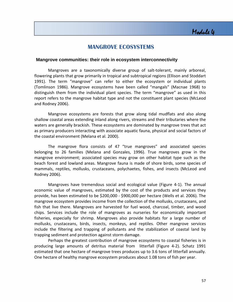
57  

Module 4

MANGROVE ECOSYSTEMS

Mangrove communities: their role in ecosystem interconnectivity  

Mangroves  are  a  taxonomically  diverse  group  of  salt‐tolerant,  mainly  arboreal, flowering plants that grow primarily in tropical and subtropical regions (Ellison and Stoddart 1991).  The  term  “mangrove”  can  refer  to  either  the  ecosystem  or  individual  plants (Tomlinson  1986). Mangrove  ecosystems  have  been  called  “mangals”  (Macnae  1968)  to distinguish  them  from  the  individual plant  species.  The  term  “mangrove”  as used  in  this report refers to the mangrove habitat type and not the constituent plant species (McLeod and Rodney 2006). 

Mangrove  ecosystems  are  forests  that  grow  along  tidal mudflats  and  also  along shallow coastal areas extending inland along rivers, streams and their tributaries where the waters are generally brackish. These ecosystems are dominated by mangrove trees that act as primary producers interacting with associate aquatic fauna, physical and social factors of the coastal environment (Melana et al. 2000). 

The  mangrove  flora  consists  of  47  “true  mangroves”  and  associated  species belonging  to  26  families  (Melana  and  Gonzales,  1996).  True  mangroves  grow  in  the mangrove  environment;  associated  species may  grow  on  other  habitat  type  such  as  the beach  forest and  lowland areas. Mangrove  fauna  is made of shore birds, some species of mammals,  reptiles, mollusks,  crustaceans,  polychaetes,  fishes,  and  insects  (McLeod  and Rodney 2006). 

Mangroves  have  tremendous  social  and  ecological  value  (Figure  4‐1).  The  annual economic  value  of mangroves,  estimated  by  the  cost  of  the  products  and  services  they provide, has been estimated to be $200,000 ‐ $900,000 per hectare (Wells et al. 2006). The mangrove ecosystem provides income from the collection of the mollusks, crustaceans, and fish  that  live  there. Mangroves  are harvested  for  fuel wood,  charcoal,  timber,  and wood chips.  Services  include  the  role  of  mangroves  as  nurseries  for  economically  important fisheries,  especially  for  shrimp. Mangroves  also  provide  habitats  for  a  large  number  of mollusks,  crustaceans,  birds,  insects,  monkeys,  and  reptiles.  Other  mangrove  services include  the  filtering  and  trapping  of  pollutants  and  the  stabilization  of  coastal  land  by trapping sediment and protection against storm damage.  

Perhaps the greatest contribution of mangrove ecosystems to coastal fisheries  is  in producing  large  amounts  of  detritus  material  from    litterfall  (Figure  4‐2).  Schatz  1991 estimated that one hectare of mangrove trees produces up to 3.6 tons of litterfall annually.  One hectare of healthy mangrove ecosystem produces about 1.08 tons of fish per year.  

 

  

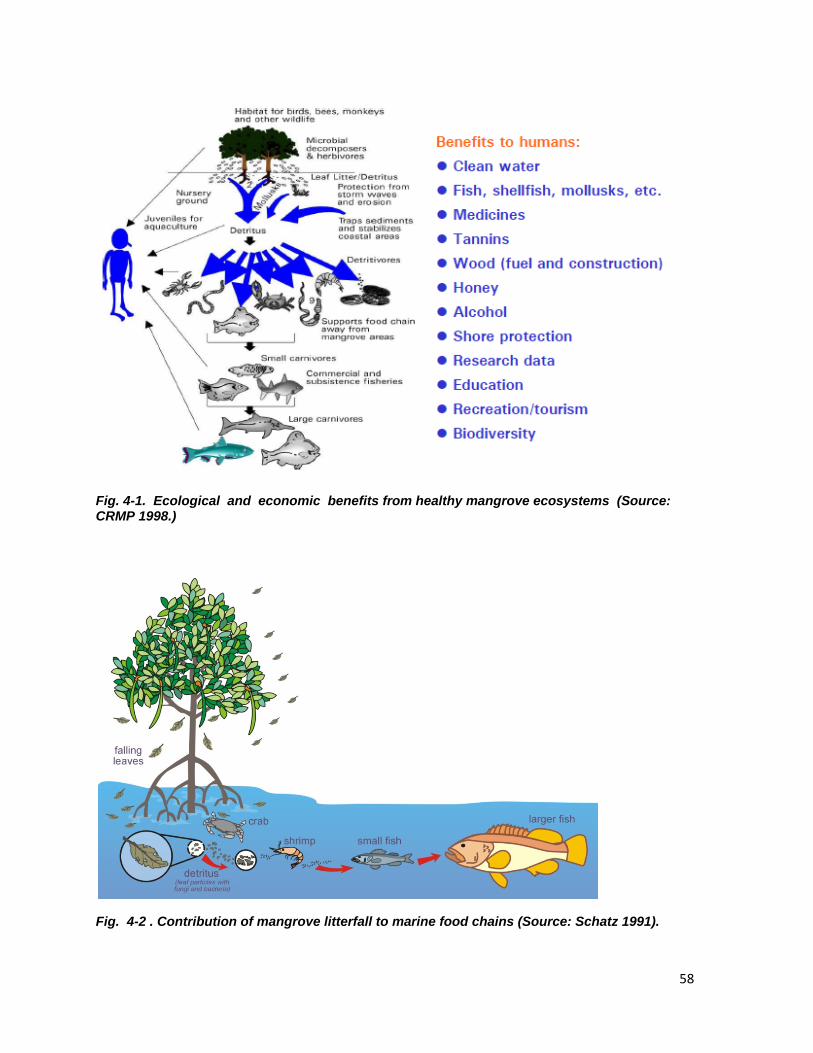
58  

Fig. 4-1. Ecological and economic benefits from healthy mangrove ecosystems (Source: CRMP 1998.)  

Fig. 4-2 . Contribution of mangrove litterfall to marine food chains (Source: Schatz 1991).

  

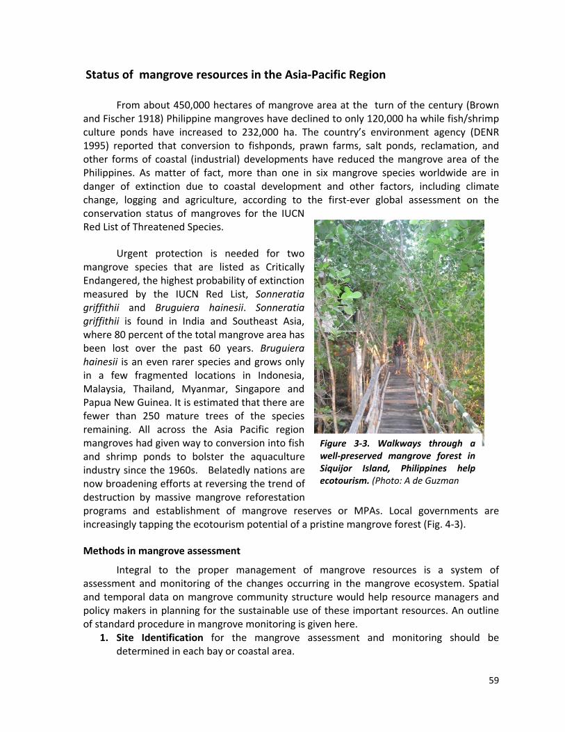
59  

Status of  mangrove resources in the Asia‐Pacific Region 

From about 450,000 hectares of mangrove area at the   turn of the century (Brown and Fischer 1918) Philippine mangroves have declined to only 120,000 ha while fish/shrimp culture  ponds  have  increased  to  232,000  ha.  The  country’s  environment  agency  (DENR 1995)  reported  that  conversion  to  fishponds,  prawn  farms,  salt  ponds,  reclamation,  and other  forms of coastal  (industrial) developments have  reduced  the mangrove area of  the Philippines.  As matter  of  fact, more  than  one  in  six mangrove  species worldwide  are  in danger  of  extinction  due  to  coastal  development  and  other  factors,  including  climate change,  logging  and  agriculture,  according  to  the  first‐ever  global  assessment  on  the conservation  status  of mangroves  for  the  IUCN Red List of Threatened Species.  

Urgent  protection  is  needed  for  two mangrove  species  that  are  listed  as  Critically Endangered, the highest probability of extinction measured  by  the  IUCN  Red  List,  Sonneratia griffithii  and  Bruguiera  hainesii.  Sonneratia griffithii  is  found  in  India  and  Southeast  Asia, where 80 percent of the total mangrove area has been  lost  over  the  past  60  years.  Bruguiera hainesii  is an even rarer species and grows only in  a  few  fragmented  locations  in  Indonesia, Malaysia,  Thailand,  Myanmar,  Singapore  and Papua New Guinea. It is estimated that there are fewer  than  250  mature  trees  of  the  species remaining.  All  across  the  Asia  Pacific  region mangroves had given way to conversion into fish and  shrimp  ponds  to  bolster  the  aquaculture industry since the 1960s.     Belatedly nations are now broadening efforts at reversing the trend of destruction  by massive mangrove  reforestation programs  and  establishment  of  mangrove  reserves  or  MPAs.  Local  governments  are increasingly tapping the ecotourism potential of a pristine mangrove forest (Fig. 4‐3).   

Methods in mangrove assessment 

  Integral  to  the  proper  management  of  mangrove  resources  is  a  system  of assessment and monitoring of  the  changes occurring  in  the mangrove ecosystem. Spatial and temporal data on mangrove community structure would help resource managers and policy makers  in planning for the sustainable use of these  important resources. An outline of standard procedure in mangrove monitoring is given here. 

1. Site  Identification  for  the  mangrove  assessment  and  monitoring  should  be determined in each bay or coastal area.   

Figure  3‐3.  Walkways  through  a well‐preserved  mangrove  forest  in Siquijor  Island,  Philippines  help ecotourism. (Photo: A de Guzman 

  

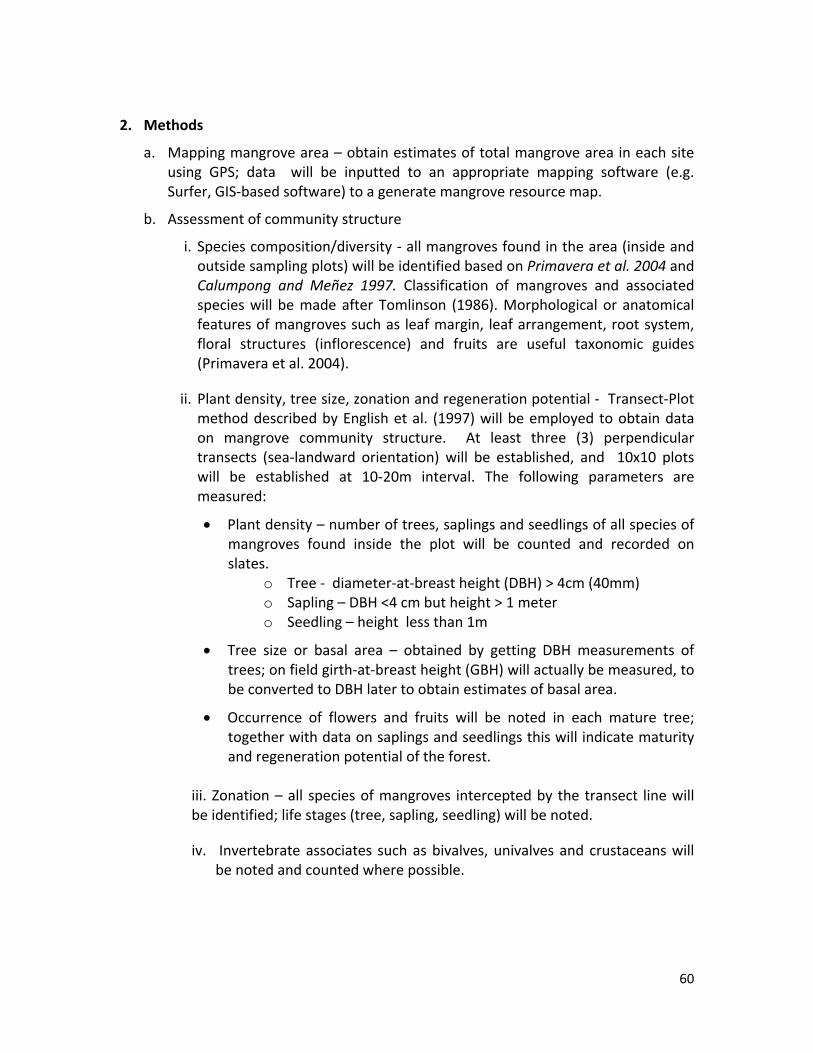
60  

 2. Methods 

a. Mapping mangrove area – obtain estimates of total mangrove area  in each site using  GPS;  data    will  be  inputted  to  an  appropriate  mapping  software  (e.g. Surfer, GIS‐based software) to a generate mangrove resource map.   

b. Assessment of community structure 

i. Species composition/diversity ‐ all mangroves found  in the area (inside and outside sampling plots) will be identified based on Primavera et al. 2004 and Calumpong  and Meñez  1997.  Classification  of mangroves  and  associated species will be made after Tomlinson  (1986). Morphological or anatomical features of mangroves such as  leaf margin,  leaf arrangement, root system, floral  structures  (inflorescence)  and  fruits  are  useful  taxonomic  guides (Primavera et al. 2004). 

ii. Plant density, tree size, zonation and regeneration potential ‐  Transect‐Plot method described by English et al.  (1997) will be employed to obtain data on  mangrove  community  structure.    At  least  three  (3)  perpendicular transects  (sea‐landward  orientation) will  be  established,  and    10x10  plots will  be  established  at  10‐20m  interval.  The  following  parameters  are measured:  

Plant density – number of trees, saplings and seedlings of all species of mangroves  found  inside  the  plot  will  be  counted  and  recorded  on slates. 

o Tree ‐  diameter‐at‐breast height (DBH) > 4cm (40mm) o Sapling – DBH <4 cm but height > 1 meter o Seedling – height  less than 1m   

Tree  size  or  basal  area  –  obtained  by  getting DBH measurements  of trees; on field girth‐at‐breast height (GBH) will actually be measured, to be converted to DBH later to obtain estimates of basal area.  

Occurrence  of  flowers  and  fruits will  be  noted  in  each mature  tree; together with data on saplings and seedlings this will indicate maturity and regeneration potential of the forest.   

 iii. Zonation – all species of mangroves  intercepted by  the  transect  line will be identified; life stages (tree, sapling, seedling) will be noted.  

iv.  Invertebrate associates  such as bivalves, univalves and crustaceans will be noted and counted where possible. 

 

  

  

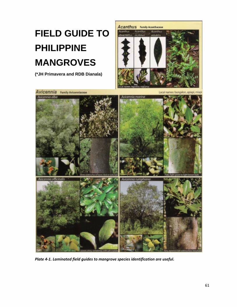
61  

FIELD GUIDE TO

PHILIPPINE

MANGROVES (*JH Primavera and RDB Dianala)

Plate 4‐1. Laminated field guides to mangrove species identification are useful.   

 

  

62  

Data Management and Analysis 

Relative Abundance (%) 

Per mangrove species:  no. plants of each species / total number of plants along the transect    x  100 

Tree, sapling, seedling:  counts per plant type/total no. in transect x 100  

Note: Present results in a pie chart  or bar chart and compare among transects or sites 

Basal Area Measurements – obtained by following these steps: 

Convert girth (circumference) measurements to diameter: dbh = c/   Example:  c = 25 cm    d = 25/3.1416 = 7.96 cm  

Calculate for basal area (per species):   A = r2  Example:  d = 7.96 cm will obtain a radius r = 3.98 

Thus, A = 3.1416 (3.98)2 or a Basal Area = 49.74 cm2  

Sum up BA for all species 

Convert to m2/hectare 

Note:  Present basal area estimates in a table or bar chart, then compare among transects or sites. 

  

 Assessing Impacts on Mangrove Ecosystems  

Table  4  shows  how  impact  on mangroves  is  assessed on  a  scale  from 0  to 5 where  0  is  no  impact  and  5  is  severely impacted. Do  this  by  looking  up  at  the  forest canopy‐ notice the average height of trees, and assess  how  many  are  at  that  level,  whether they  touch  and  overlap  (code  0)  or  whether there  are  gaps  between  them  (English  et  al. 1997).  Other  impacts  or  threats  such  as  tree cutting  and  garbage  pile  up  should  also  be noted  (see    Table  5).  Noteworthy  too  are 

mangrove reforestation efforts  in the site. For example, many well‐meaning rehabilitation efforts involve planting monospecific seedlings in inappropriate location or substrata, often times ending in wasted money and manpower investment.  

Figure  4‐4.  Natural and human impacts can threaten a pristine mangrove forest such as this (Photo: AB de Guzman)  

  

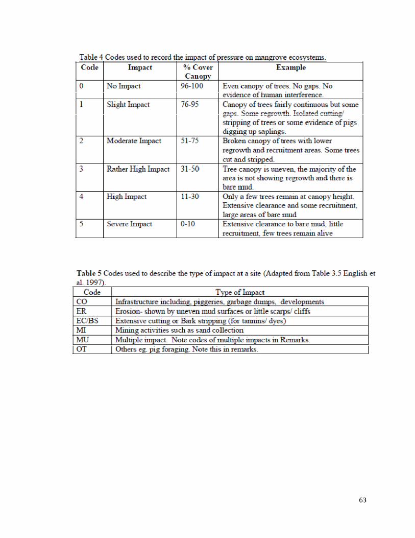
63  

 

  

64  

Main References 

 

Agostini, S. 2003. Distribution and estimation of basal area coverage of subtidal seagrass meadows 

in a Mediterranean coastal lagoon.  Estuarine Coastal Shelf Science 56:1021‐1028 

Aliño,  P.M.,  H.O  Arceo, N.  Palomar,  and  A.J. Uychiaoco.  2000.  Challenges  and Opportunities  for Community  Participation  for  the Management  of Marine  Protected  Areas  (MPAs)  in  the Philippines. Paper presented on the 9th International coral Reef Symposium, Bali, Indonesia. 23‐27 October 2000.  

Brown, W.H., and A.F. Fischer. 1918. Philippine mangrove swamps. Department of Agriculture and Natural Resources. Bureau of Fishery Bulletin No. 7. 

Burke. L., E. Selig and M. Spalding. 2002. Reefs at Risk in Southeast Asia. World resources Institute, Washington, DC, USA. 72pp 

Cheung, C.. P. Aliño, A.J. Uychiaoco, and H. Arceo. 2002. Marine Protectead Areas in Southeast Asia. ASEAN Regional Center for Biodiversity Conservation. Department of Environment and Natural Resources, Los Baños, Philippines. pp.3‐5 

Den Hartog, C. 1970. The seagrasses of the world. North Holland, Amsterdam. 

DENR, DA‐BFAR and DILG. 2001. Philippine coastal management guidebook series (nos. 1‐8). Coastal Resource Management Project of the DENR, Cebu City, Philippines. 

DENR Statistics. 1995. Environment and Natural Resources Atlas of the Philippines. Published by the Environment center of The Philippines Foundation.  1998. Manila, Philippines. 

Duffy, E.J. 2006. Biodiversity and the functioning of seagrass ecosystems. Marine Ecology Progress Series, 311:233‐250. 

Ellison, J.C. and D.R. Stoddart. 1991. Mangrove ecosystem collapse during predicted sea‐level rise: Holocene analogues and implications. Journal of Coastal Research 7: 151‐165. 

English,  S.,  C. Wilkinson  and  V.  Baker.  1997,  Survey Manual  for  Tropical Marine  Resources,  2nd Edition. (Townsville: Australian Institute of Marine Science).  

Fortes, M.D. 1989. Seagrass: A resource unknown in the ASEAN region. ICLARM Education Series 5, International Center of Living Aquatic Resources Management, Manila, Philippines. p.46  

Fortes,  M.D.  1990.  Seagrass‐mangrove  ecosystems  management:  a  key  to  marine  coastal conservation in the ASEAN region. Marine pollution Bulletin. 23:113‐116. 

Hemminga, M.A. and C.M. Duarte. 2000. Seagrass Ecology. Edinburgh building, Cambridge CB2 2RU, United Kingdom at the University Press, Cambridge. pp. 298.  

Kenchington,  R.A.,  1978.  Visual  surveys  of  large  areas  of  coral  reefs.  In  Coral  Reefs:  Research Methods, edited by D.R. Stoddart and R.E. Johannes (Paris: UNESCO),pp. 149–161.  

Kuiter,  R.H.  and  H.  Debelius.  2006.  World  Atlas  of  Marine  Fishes.  IKAN‐Unterwasserarchive, Waldschultsrasse 166, 65933 Frankfurt, Germany. 

Licuanan WY, Gomez ED. 2000. Philippine coral reefs: status and the role of the academe to improve their management. Proc 9th Int Coral Reef Symp, Bali, Indonesia 2:835‐840. 

Macnae, W. 1968. A general account of the fauna and flora of mangrove swamps and forests in the Indo‐West‐Pacific region. Advances in Marine Biology 6:73‐270. 

  

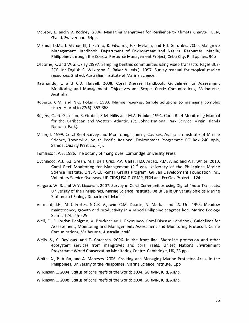
65  

McLeod, E. and S.V. Rodney. 2006. Managing Mangroves  for Resilience  to Climate Change.  IUCN, Gland, Switzerland. 64pp. 

Melana, D.M.,  J. Atchue  III, C.E. Yao, R. Edwards, E.E. Melana, and H.I. Gonzales. 2000. Mangrove Management  Handbook.  Department  of  Environment  and  Natural  Resources,  Manila, Philippines through the Coastal Resource Management Project, Cebu City, Philippines. 96p  

Osborne, K. and W.G. Oxley .1997. Sampling benthic communities using video transects. Pages 363‐376.  In:  English  S, Wilkinson  C,  Baker  V  (eds.).  1997.  Survey manual  for  tropical marine resources. 2nd ed. Australian Institute of Marine Science. 

Raymundo,  L.  and  C.D.  Harvell.  2008.  Coral  Disease  Handbook;  Guidelines  for  Assessment Monitoring  and  Management:  Objectives  and  Scope.  Currie  Comunications, Melbourne, Australia.  

Roberts,  C.M.  and  N.C.  Polunin.  1993. Marine  reserves:  Simple  solutions  to managing  complex fisheries. Ambio 22(6): 363‐368. 

Rogers, C., G. Garrison, R. Grober, Z‐M. Hillis and M.A. Franke. 1994, Coral Reef Monitoring Manual for  the  Caribbean  and Western  Atlantic.  (St.  John:  National  Park  Service,  Virgin  Islands National Park).   

Miller,  I. 1999. Coral Reef Survey and Monitoring Training Courses. Australian  Institute of Marine Science,  Townsville.  South  Pacific  Regional  Environment  Programme  PO  Box  240  Apia, Samoa. Quality Print Ltd, Fiji. 

Tomlinson, P.B. 1986. The botany of mangroves. Cambridge University Press. 

Uychiaoco, A.J., S.J. Green, M.T. dela Cruz, P.A. Gaite, H.O. Arceo, P.M. Aliño and A.T. White. 2010. Coral  Reef  Monitoring  for  Management  (2nd  ed).  University  of  the  Philippines  Marine Science  Institute, UNEP, GEF‐Small Grants Program, Guiuan Development Foundation  Inc., Voluntary Service Overseas, UP‐CIDS,USAID‐CRMP, FISH and EcoGov Projects. 124 p.   

Vergara, W. B. and W.Y. Licuayan. 2007. Survey of Coral Communities using Digital Photo Transects. University of the Philippines, Marine Science Institute. De La Salle University Shields Marine Station and Biology Department‐Manila. 

Vermaat,  J.E., M.D.  Fortes,  N.C.R.  Agawin.  C.M.  Duarte,  N. Marba,  and  J.S.  Uri.  1995. Meadow maintenance, growth and productivity  in a mixed Philippine seagrass bed. Marine Ecology Series, 124:215‐225 

Weil, E., E.  Jordan‐Dahlgren, A. Bruckner ad L. Raymundo. Coral Disease Handbook; Guidelines  for  Assessement, Monitoring and Management; Assessment and Monitoring Protocols. Currie Comunications, Melbourne, Australia. pp48. 

Wells  ,S.,  C.  Ravilous,  and  E.  Corcoran.  2006.  In  the  front  line:  Shoreline  protection  and  other ecosystem  services  from  mangroves  and  coral  reefs.  United  Nations  Environment Programme World Conservation Monitoring Centre, Cambridge, UK, 33 pp. 

White, A., P. Aliño, and A. Meneses. 2006. Creating and Managing Marine Protected Areas  in  the Philippines. University of the Philippines, Marine Science Institute.  1pp  

Wilkinson C. 2004. Status of coral reefs of the world: 2004. GCRMN, ICRI, AIMS. 

Wilkinson C. 2008. Status of coral reefs of the world: 2008. GCRMN, ICRI, AIMS.   

  

66  

Appendix 1.  Glossary of terms often used in coral reef monitoring. 

 

  

67