Trajectory Clustering, Modelling, and Selection with the focus on

Airspace Protection

Willem J. Eerland ∗ and Simon Box †

University of Southampton, Southampton, England SO17 1BJ, United Kingdom

March 31, 2016

Abstract

Take-off and landing are the periods of a flight where aircraft are most vulnerable to a groundbased rocket attack by terrorists. While aircraft approach and depart from airports on pre-definedflight paths, there is a degree of uncertainty in the trajectory of each individual aircraft. Capturingand characterizing these deviations is important for accurate strategic planning for the defence ofairports against terrorist attack. A methodology is demonstrated whereby approach and departuretrajectories to a given airport are characterized statistically from historical data. It uses a two-stepprocess of first clustering to extract the common trend, and then modelling uncertainty using GaussianProcesses (GPs). Furthermore it is shown that this approach can be used to either select probabilisticregions of airspace where trajectories are likely and - if required - can automatically generate a setof representative trajectories, or select key trajectories that are both likely and critically vulnerable.An evaluation of the methodology is demonstrated on an example data-set collected by the groundradar at an airport. The evaluation indicates that 99.8% of the calculated footprint underestimatesless than 5% when replacing the original trajectory data with a set of representative trajectories.

1 Introduction

Extracting patterns from data is an active field for both research and industry, ranging from trackingtraffic to making predictions on the financial market. It allows for objects to be clustered when

following a similar trend. And by identifying the generic response, an attempt can be made to explainthese reactions. When it comes to air traffic, the reason is well known. As an aircraft enters controlledairspace, such as near an airport, they follow the instructions of air traffic control, who guide them alongpre-designated paths.

In the real-world, these pre-designated paths, also called flight paths, have more resemblance tocorridors. For this reason, the current methodology on calculating noise contours around civil airportsin Europe, uses several sub-tracks to model the dispersion along a single flight path [3]. When using theIntegrated Noise Model (INM) [2] to calculate the noise contours, either the sub-tracks or dispersion willhave to be supplied by the user. Nowadays, with the air traffic increasing in volume, the introduction ofnew technologies and procedures being developed under the names NextGen and SESAR, the dispersionalong the flight paths is more susceptible to change than ever before. A step-by-step guide to obtaina number of representative trajectories from historical data (over any given time-frame or conditions),is able to reduce the computational load in any subsequent analysis, without losing integrity and withlimited effort for the user.

While noise can literally keep people awake at night, it is nowhere near as vital as securing theinfrastructure. More specifically, protecting aircraft against the threat from Rocket-Propelled Grenades(RPGs), that can hit a moving target up to a distance of 300 metres [1]. The threat is real, as actions inthe past, such as the heightened security around Heathrow back in 2003 have shown [8]. This is one ofthe reasons governments, airports and airliners alike perform much strategic planning to defend aircraftfrom terrorists attacks. In the scenario where the computational budget is limited, possibly due to themultitude of scenarios to evaluate or a time restriction, evaluating all the trajectories is not always aviable option. Having a method to determine, in a robust statistical manner, where the aircraft are mostlikely to be, is the first step in efficiently identifying high-risk launch sites.

Focussing on the work done in the aerospace sector, there have already been great advances in auto-matically clustering of aircraft trajectories on a common flightpath. One clustering method re-samples

∗Postgraduate researcher, Transportation Research Group, w.j.eerland@soton.ac.uk†Lecturer, Transportation Research Group

1

arX

iv:1

603.

0920

8v1

[st

at.A

P] 3

0 M

ar 2

016

this is a pre-print of the paper published in Infotech, AIAA SciTech 2016found at: http://dx.doi.org/10.2514/6.2016-1411

data

cluster 1

model

trajectories

cluster . . . cluster n

Figure 1: Procedure to obtain representative trajectories based on data.

the trajectories to fit in a vector of fixed size, after which the size of the vector is reduced using Princi-ple Component Analysis (PCA). The data are then clustered using Density-Based Spatial Clustering ofApplications (DBSCAN) [7], or k-means clustering [4]. Here the DBSCAN [6] allows for the filtering ofoutliers, resulting in a more robust clustering method compared to using k-means clustering. Anotherinteresting method used to cluster the aircraft trajectories is based on Fourier coefficients [9]. The majordifference here is that the trajectories are not merely re-sampled, but represented as Fourier-coefficientsthat effectively parametrises the aircraft trajectories. However, it should be said that the parametrisationis limited here to two spatial dimensions, ignoring the vertical variation in the flight-paths.

Automatic clustering (i.e. discovery of flight-paths) is an important first step, however, it holds littleinformation about the level of dispersion of the trajectories within a given cluster, i.e. around the nominalflight-path. A method has been proposed by Salaun et al.[11] to calculate the probabilities by re-sampling,and fitting a univariate Gaussian in both the lateral and vertical direction perpendicular to the meantrajectory. Using this approach, they were successful in creating a tunnel through which a percentage ofaircraft trajectories manoeuvre. More recently, a similar approach of modelling trajectories as GaussianProcesses (GPs) has been developed by the authors[5]. This allows the aircraft trajectories to be treatedin a continuous manner and also models the covariance between the lateral and vertical direction.

In this paper, we present a step-by-step method to replace a large data-set of historical trajectories,with a number of representative trajectories that have none-the-less captured the dispersion in the originallarge data-set. The trajectory data are clustered, after which a probabilistic model is generated for eachindividual cluster. This probabilistic model is then used to generate weighted representative trajectories,each capturing a fraction of the whole cluster. The aim here is to reduce the computational cost ofcalculations that are done in sub-sequential steps. Such calculations can be either focussed on calculatingnoise footprints, or be aimed at performing a strategic analysis with the focus on safeguarding the airspaceinfrastructure. The latter is evaluated to demonstrate the effectiveness of the proposed method whengenerating a footprint on ground level.

This paper is organised as follows. In section 2, each step is explained, resulting in a guide how totransform the original trajectory data into a set of weighted representative trajectories. Next, in section 3,the methods are applied in a case study. This includes in an evaluation to compare the original trajectorydata with a set of representative trajectories. The set of representative trajectories are generated in twoways, one takes into account the dispersion in lateral direction only, while the other also includes thevertical dispersion. Finally, in section 4, we conclude the paper with remarks and recommendations forfuture work.

2 Methods

This section reviews the techniques used to replace historical data with representative trajectories. Thefirst part focuses on clustering the trajectory data by identifying groups of trajectories with similarflight-path. The second part focuses on estimating the dispersion of each individual cluster along theflight-path. The third and final part is aimed at creating weighted trajectories that represent the aircrafttrajectories flying through the airspace. The complete procedure is seen in fig. 1, where the data are firstclustered, then modelled and finally representative trajectories are generated (leaving the possibility ofselection).

2.1 Clustering the Trajectories

In order to cluster the trajectories based on a common flightpath, it is assumed that in the referenceframe, the location of the runways are known and there is a human-in-the-loop, i.e. the process is notfully automated. The clustering technique takes the shape of the following three-step approach:

2

this is a pre-print of the paper published in Infotech, AIAA SciTech 2016found at: http://dx.doi.org/10.2514/6.2016-1411

1. clustering trajectories as approach or departure

2. clustering the trajectories by run-way

3. re-sampling of trajectories

4. dimension reduction with PCA

5. DBSCAN clustering

The first step distinguishes the trajectory data between approach and departure. In the case where thesemeta-data are not included, the location of the airport is sufficient to identify whether a trajectory eitherends at the airport (approach), or is leaving (departure). E.g. if the Euclidean distance between theairport and the first point of the trajectory is smaller than the Euclidean distance between the airportand the last point of the trajectory, it is likely to be a departure. The second step requires informationabout the location of the runway in a similar reference frame as the trajectories. While it reduces thegenerality, it does allow for a clean separation per runway.

Steps 3−5 are mostly similar to the procedure as presented in Gariel et al.[7]. In step 3 the trajectoriesare re-sampled to a vector of a fixed size using uniform spacing based on the index number. Note thatre-sampling over 30 steps result in a [1 × 90] vector as aircraft trajectories have 3 dimensions, and thedimensions are concatenated. Furthermore, the re-sampling is done per individual trajectory, while thenext step, the reduction of the vector size, considers the entire data-set. Next, in step 4, these vectorsare reduced in size using PCA. Here the principle components with the largest variance are kept, whilethe components with little variation are ignored. In this step it is assumed that the components withthe largest variation are most important for the clustering. The clustering occurs in the final step, wherethe trajectories are clustered using DBSCAN. Here, the ε-neighbourhood parameter ε of the DBSCANalgorithm needs to be set on a case-by-case basis, a smaller ε will result in more clusters with fewertrajectories, whereas with a larger ε results in less clusters with more trajectories. In the final step allclusters with less than a user-specified number of trajectories will be ignored, effectively removing theoutliers.

2.2 Modelling the Spatial Distribution

In this section a short overview of the modelling technique is provided. For a complete description, pleasesee Eerland and Box[5]. Essentially, there are two steps in modelling the spatial distribution:

• normalising the trajectory data (per cluster, see previous section)

• learn model parameters via maximum likelihood estimation

The first step assures that the dimensions are of the same scale. In particular for aircraft trajectoriesthis is an important step, as usually the distance covered horizontally is much larger than the distancetravelled vertically. When estimating the parameters, this can lead to computational problems, as such,the trajectory data are normalised such that each dimension fits on a [0, 1] range. This transformationcan be reverted once the model has been created. Furthermore, normalised time τ is introduced to alignall points of the trajectories at the start at the end. The start is set to be τ = 0 and the end is τ = 1,where the points in between are set proportionally. E.g. if the first point occurs at 0 seconds and thelast point occurs at 20 seconds, the point at 12 seconds will have the normalised time τ = 12/20 = 0.6.As such, each point in the trajectory is described as a 3× 1 vector y(τ), holding eastings, northings andaltitude at the normalised time τ .

In the second step the model parameters are estimated. Here the parameters consist of the meanfunction m(τ), covariance kernel k(τ, τ ′) and noise precision term β. These parameters capture theunderlying function y(τ) according to the following relation:

y(τ) ∼ GP(m(τ),k(τ, τ ′)) (1)

wherem(τ) = E[y] = φ(τ)µ (2)

k(τ, τ ′) = E[(y(τ)−m(τ))(y(τ ′)−m(τ ′))] = φ(τ)Σφᵀ(τ ′) + β−1I (3)

In these equations the mean function m(τ) and the covariance kernel k(τ, τ ′) are captured using J basisfunctions. Here the discrete number of parameters captured in the 3J × 1 vector µ and 3J × 3J matrixΣ, are converted from the discrete domain to the continuous domain via the block-diagonal 3×J matrix

3

this is a pre-print of the paper published in Infotech, AIAA SciTech 2016found at: http://dx.doi.org/10.2514/6.2016-1411

φ(τ). The basis functions φ(τ) consists of 3 blocks, corresponding with the number of dimensions foundin aircraft trajectories.

Next, for the estimation the Expectation-Maximisation (EM) algorithm is applied, this deals withthe chicken-egg paradigm. More specifically, β is needed to estimate m(τ) and k(τ, τ ′), and m(τ) andk(τ, τ ′) are needed to estimate β. Basically, each individual trajectory is captured in the model describedby the couple m(τ) and k(τ, τ ′), however not perfectly, thus the remaining error is captured in β. Andby doing so, maximizing the likelihood of these three terms using EM, prevents the probabilistic modelto over-fit on the data (assuming the remaining error is Gaussian distributed).

Initially µ (a 3J × 1 vector) is assumed 0, and Σ (a 3J × 3J matrix) is assumed aI, where I is theidentity matrix and a an arbitrarily large number. This represents a not very informative prior andreflects the concept that no initial knowledge is available. The noise precision term β can be set high(e.g. in the order of magnitude of 103), to reflect that the measurements are exact and the remainingerror low.

Using these initial parameters, the expected parameter values w (the E-step of the EM algorithm)are:

E[wn] = Sn(βφᵀnyn + Σ−1µ) (4)

E[wnwᵀn] = Sn + E[wn]E[wᵀ

n] (5)

whereS−1n = Σ−1 + βφᵀ

nφn (6)

In these equations n represents the individual trajectory, and N equates the total number of trajectoriesfound in the cluster.

Next, the likelihood is maximized with respect to the model parameters (the M-step of the EMalgorithm) using:

µ̂ =1

N

N∑n=1

{E[wn]} (7)

Σ̂ =1

N

N∑n=1

{E[wnwᵀn]− 2E[wᵀ

n]µ + µµᵀ} (8)

1

β̂=

1

3M∗

N∑n=1

{yᵀnyn − 2yᵀ

n(φnE[wn]) + Tr(φᵀnφnE[wnwᵀ

n])} (9)

where the hat seen in µ̂, Σ̂ and β̂ signifies an approximation. These two steps in the EM algorithm arerepeated until the likelihood is converged, where the negative log-likelihood itself can be evaluated using:

− lnL = −3M∗

2ln(β) +

β

2

N∑n=1

{yᵀnyn − 2yᵀ

n(φnwn) + Tr(φᵀnφnwnwᵀ

n)}

+N

2ln(|Σ|) +

1

2

N∑n=1

{Tr(Σ−1(wnwᵀn − 2wᵀ

nµ + µµᵀ))} (10)

where

M∗ =

N∑n=1

{Mn} (11)

and Mn represents the total number of points in yn, thus M∗ embodies the total number of points in theentire cluster.

The difference between two sequential log-likelihood evaluations is used as a stopping criteria, at thispoint the model approximation is assumed sufficient. Due to the nature of the EM algorithm, it willalways be considered an approximation.

The approximated parameters can now be interested in the model, seen in eq. (1), to estimate theprobabilistic model at any τ in the domain τ = [0, 1]. This model allows itself to be expressed in a mul-tivariate Gaussian distribution as a function of τ , which will be used to generate weighted representativetrajectories in the next section.

4

this is a pre-print of the paper published in Infotech, AIAA SciTech 2016found at: http://dx.doi.org/10.2514/6.2016-1411

2.3 Generating representative trajectories

The previous section described how to estimate the probabilistic model. This section provides a methodto convert this model to weighted trajectories that represent the entire cluster.

For a 3-dimensional vector y(τ), the multivariate Gaussian distribution takes the form:

N (m,k) =1√

(2π)3/21

|k|1/2exp

{−1

2MD(y,m,k)

}(12)

where MD represents the Mahalanobis distance:

MD(y,m,k)) = (y −m)ᵀk−1(y −m) (13)

And note that the dependence on τ has been dropped for readability.Furthermore, at a constant Mahalanobis distance, this equation takes the form of an ellipsoid described

by |k|−1/2, centred at m. In this scenario the axes of the covariance ellipse are given by the eigenvectorsr of the covariance kernel k. The corresponding lengths, for an ellipse with unit Mahalanobis radius, aregiven by the square roots of the corresponding eigenvalues λ. Both can be found using the eigenvaluedecomposition of the matrix k.

RΛR−1 = k (14)

whereR = [r1 r2 r3] (15)

and

Λ =

λ1 0 00 λ2 00 0 λ3

(16)

In short, the shape of the ellipsoid is described by the eigenvalues found in Λ, where m and R are merelya translation and rotation respectively. The equation for the ellipsoid is given by:

y21λ1

+y22λ2

+y23λ3

= 1 (17)

The plane perpendicular to the mean function at time τ , can be described with a unit normal vectorn. As m(τ) is continuous, this unit normal vector n can be both derived, or calculated numerically:

n =m(τ + dτ/2)−m(τ − dτ/2)

dτ(18)

where dτ is an arbitrarily small number. The mathematics required to calculate the intersection betweenthe plane and ellipsoid is given in Klein [10]. By doing so, the two-dimensional ellipse can be evaluatedat any angle. However, it’s important to note that the plane generated at time τ intersects multipleellipsoids, it’s therefore necessary to evaluate all those that intersect and store the point correspondingwith the largest deviation from the centre point (provided by m(τ)).

To obtain a representative trajectory, the ellipse at any specific angle, which is a single point in athree-dimensional space, can be evaluated over τ = [0, 1] in any number of steps. In this paper 100 stepsare used. Thus the combination of a constant Mahalanobis distance (representing a confidence interval,to be discussed next) and a given angle provides one representative trajectory. However, when it comesto selecting the angles to obtain a selection of representative trajectories, there are an infinite number ofoptions. In this paper two options are compared. In the handbook on generating noise contours [3], onlythe dispersion in lateral direction is taken into account. Here the cross-section containing the artificialtrajectories appears like fig. 2(a), where the Gaussian distribution is included as a reference. In this figure,5 trajectories are shown to capture a given percentage (the area under the curve). This corresponds withthe Cumulative Distribution Function (CDF), which is equal to chi-square with 1 degree of freedom.The resulting weight per trajectory is shown in table 1. The area under the curve described by theGaussian corresponds with a confidence interval (thus capturing a certain percentage of the completedata) - and this percentage is divided over multiple trajectories due to symmetry. E.g. for the caseof lateral dispersion only, in the range [0.52, 1.52], the total percentage 48.3461% is divided over twotrajectories centred at a standard deviation of one (N = 2), resulting in 24.1730% per trajectory. Whenincluding the vertical dispersion, the model show more similarity to fig. 2(b). As it now encompassestwo dimensions, the chi-square with 2 degrees of freedom is used. Combined with angles at variousranges, there are 17 representative trajectories. The weight per trajectory is shown in table 2. In theevaluations seen further on in this paper, these percentages will be multiplied with the total traffic toobtain representative number of trajectories. I.e. the percentages shown here, are the weights used inthe calculations.

5

this is a pre-print of the paper published in Infotech, AIAA SciTech 2016found at: http://dx.doi.org/10.2514/6.2016-1411

Table 1: Weights generated using the chi-square distribution table (1 degree of freedom).range total percentage percentage per

captured trajectory[0.02, 0.52] 38.29% 38.29% (N = 1)[0.52, 1.52] 48.35% 24.17% (N = 2)[1.52, 2.52] 12.12% 6.06% (N = 2)[0.02, 2.52] 98.76% 98.76% (N = 5)

Table 2: Weights generated using the chi-square distribution table (2 degrees of freedom).range total percentage percentage per

captured trajectory[0.02, 0.52] 11.75% 11.75% (N = 1)[0.52, 1.52] 55.78% 6.97% (N = 8)[1.52, 2.52] 28.07% 3.51% (N = 8)[0.02, 2.52] 95.61% 95.61% (N = 17)

2 1 0 1 2

(a) Cross-section of the representativetrajectories (indicated by blue dots),when only taking the lateral dispersioninto account. At the top is a schematicrepresentation of the Gaussian distribu-tion, placed as a reference.

(b) Cross-section of the representativetrajectories (indicated by blue dots)when taking both the lateral and verticaldispersion into account.

Figure 2: Two options to obtain representative trajectories.

6

this is a pre-print of the paper published in Infotech, AIAA SciTech 2016found at: http://dx.doi.org/10.2514/6.2016-1411

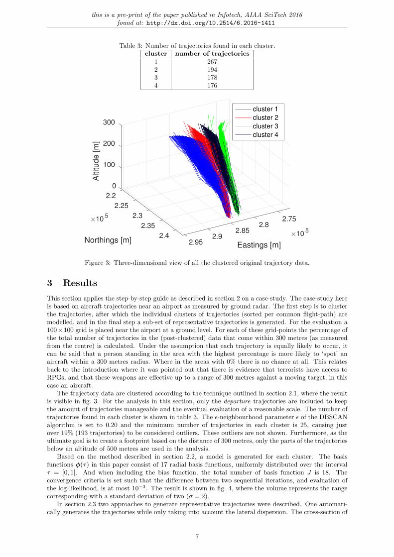
Table 3: Number of trajectories found in each cluster.cluster number of trajectories

1 2672 1943 1784 176

0

2.2

100

2.25

2.3

Altitude [m

]

Northings [m]

×105

2.75

200

2.82.35

Eastings [m]

×1052.85

300

2.4 2.92.95

cluster 1

cluster 2

cluster 3

cluster 4

Figure 3: Three-dimensional view of all the clustered original trajectory data.

3 Results

This section applies the step-by-step guide as described in section 2 on a case-study. The case-study hereis based on aircraft trajectories near an airport as measured by ground radar. The first step is to clusterthe trajectories, after which the individual clusters of trajectories (sorted per common flight-path) aremodelled, and in the final step a sub-set of representative trajectories is generated. For the evaluation a100×100 grid is placed near the airport at a ground level. For each of these grid-points the percentage ofthe total number of trajectories in the (post-clustered) data that come within 300 metres (as measuredfrom the centre) is calculated. Under the assumption that each trajectory is equally likely to occur, itcan be said that a person standing in the area with the highest percentage is more likely to ‘spot’ anaircraft within a 300 metres radius. Where in the areas with 0% there is no chance at all. This relatesback to the introduction where it was pointed out that there is evidence that terrorists have access toRPGs, and that these weapons are effective up to a range of 300 metres against a moving target, in thiscase an aircraft.

The trajectory data are clustered according to the technique outlined in section 2.1, where the resultis visible in fig. 3. For the analysis in this section, only the departure trajectories are included to keepthe amount of trajectories manageable and the eventual evaluation of a reasonable scale. The number oftrajectories found in each cluster is shown in table 3. The ε-neighbourhood parameter ε of the DBSCANalgorithm is set to 0.20 and the minimum number of trajectories in each cluster is 25, causing justover 19% (193 trajectories) to be considered outliers. These outliers are not shown. Furthermore, as theultimate goal is to create a footprint based on the distance of 300 metres, only the parts of the trajectoriesbelow an altitude of 500 metres are used in the analysis.

Based on the method described in section 2.2, a model is generated for each cluster. The basisfunctions φ(τ) in this paper consist of 17 radial basis functions, uniformly distributed over the intervalτ = [0, 1]. And when including the bias function, the total number of basis function J is 18. Theconvergence criteria is set such that the difference between two sequential iterations, and evaluation ofthe log-likelihood, is at most 10−3. The result is shown in fig. 4, where the volume represents the rangecorresponding with a standard deviation of two (σ = 2).

In section 2.3 two approaches to generate representative trajectories were described. One automati-cally generates the trajectories while only taking into account the lateral dispersion. The cross-section of

7

this is a pre-print of the paper published in Infotech, AIAA SciTech 2016found at: http://dx.doi.org/10.2514/6.2016-1411

Figure 4: Three-dimensional view of all models - where the volume corresponds with a standard deviationof two.

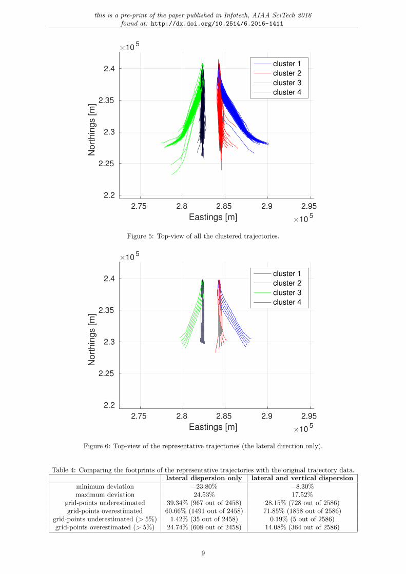
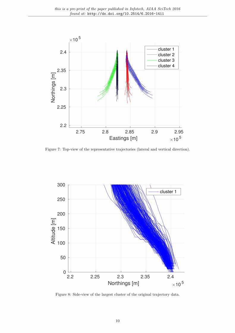
this ‘flat’ version is seen in fig. 2(a), and the resulting top-view is visible in fig. 6. This modelling approachis currently being used in calculating noise footprints around airports, as described in the official publi-cation [3]. The other approach takes into account both the lateral and vertical dispersion simultaneously.The cross-section of this ‘round’ version is seen in fig. 2(b), and the resulting top-view is visible in fig. 7.

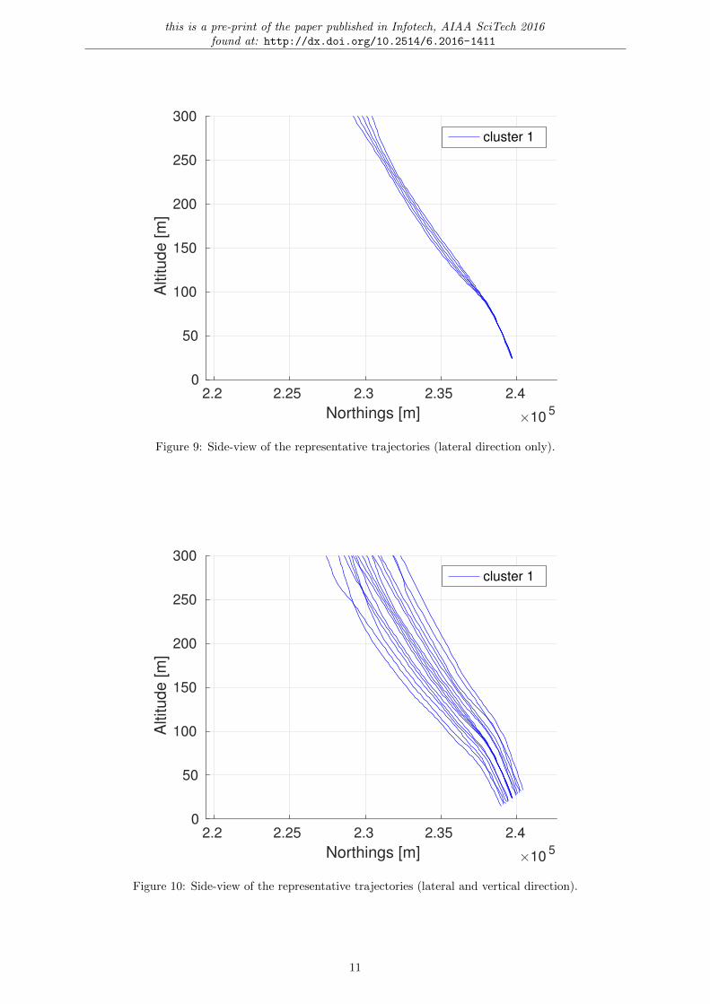
The difference by taking into account the vertical dispersion becomes apparent when examining theside-views seen in figs. 8 to 10, where the original trajectory data and the two version of representativetrajectories are displayed. It clearly shows that modelling the vertical dispersion, actually represents thevertical dispersion as seen in the original data.

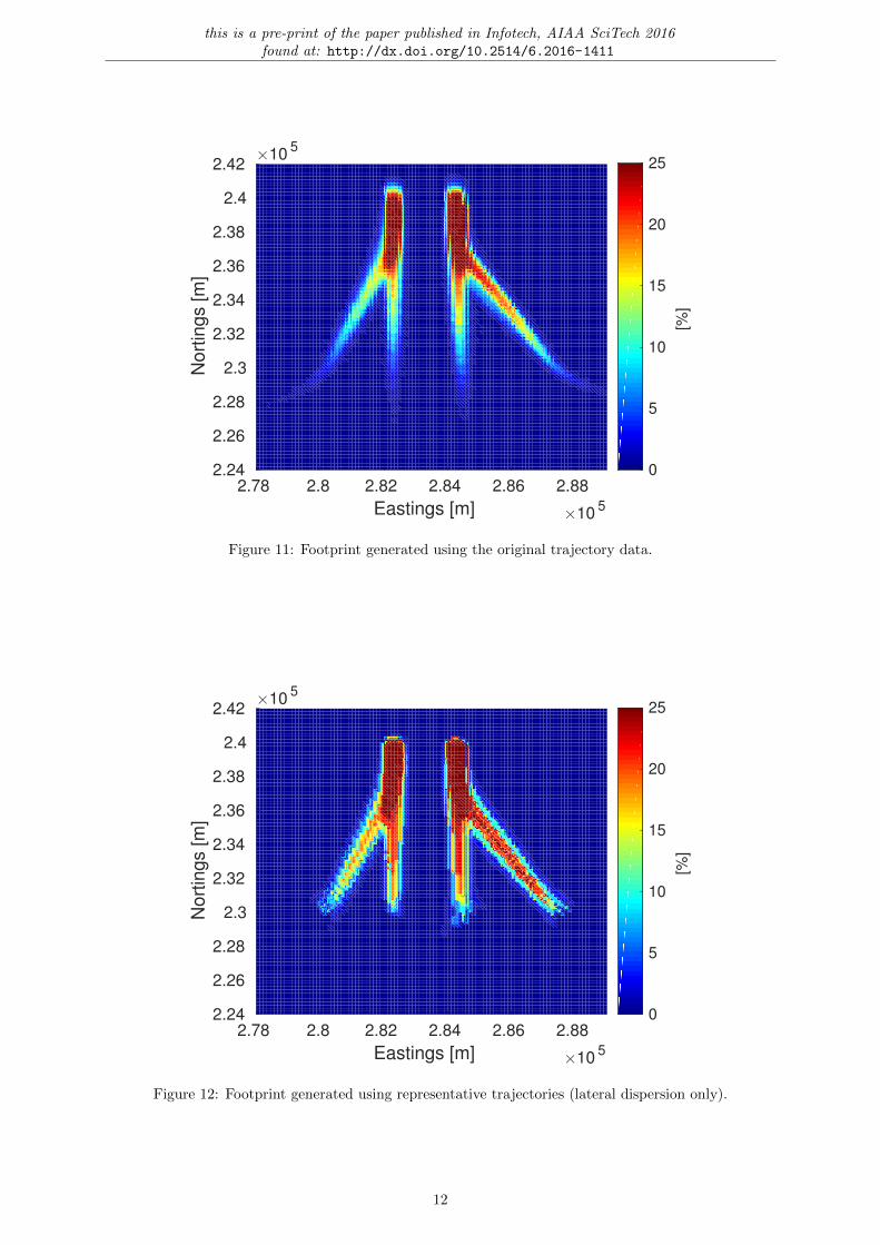
For the evaluation a 100 × 100 grid is placed near the airport at a ground level. For each of thesegrid-points the percentage of the 815 trajectories in the data that come within 300 metres is calculated.This simulates a simplistic approach to calculate from which locations the aircraft are vulnerable to anattack using RPGs, without taking into account any mapping nor specific weapon characteristics. Forcomparison, the analysis is performed on the original trajectory and the two versions of the representativetrajectories.

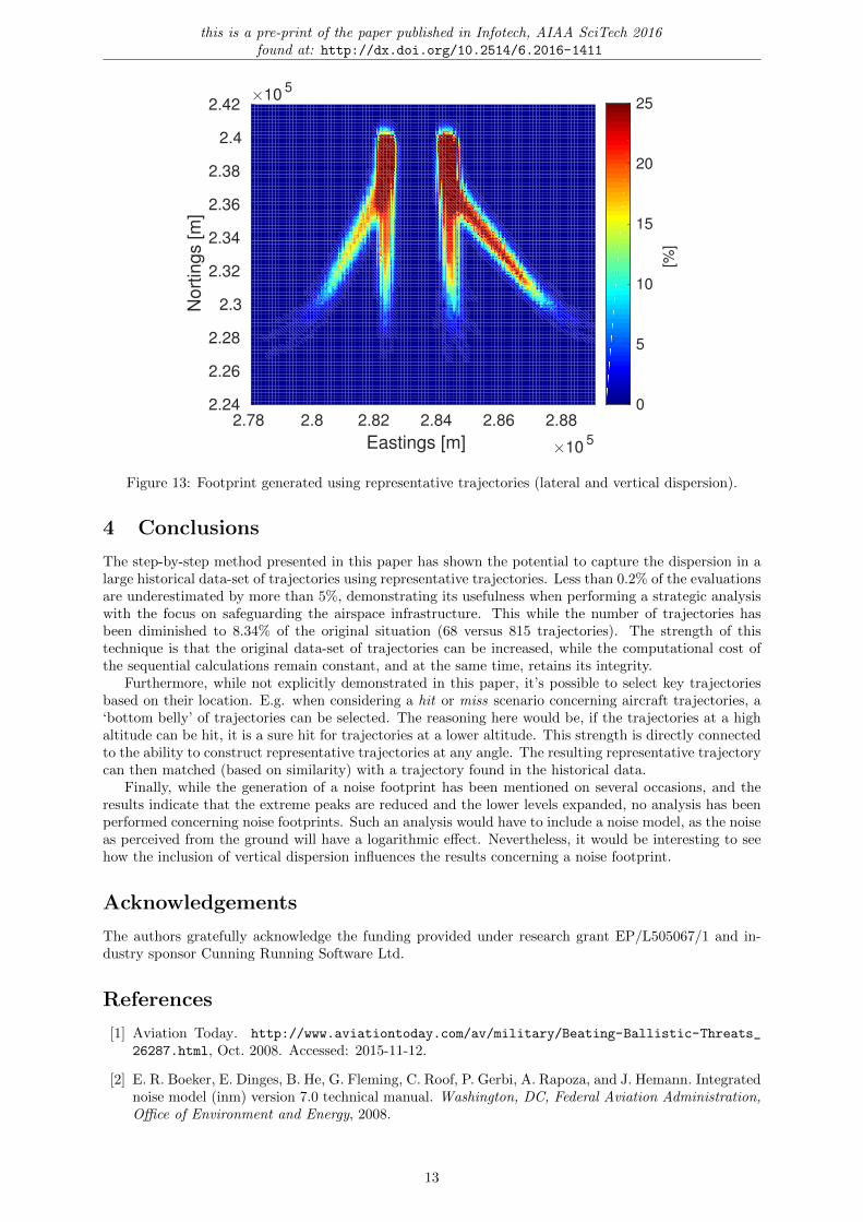
The resulting footprint calculated for the original trajectory data is visible in fig. 11, where the rangeof percentages has been set to visualise the sweep of low percentages towards the end. This sweep ismissing from fig. 12, where only the lateral dispersion is taken into account. While the visible roughnessis a direct effect of only using 5 trajectories to represent each cluster, the missing sweep is a directresult of missing trajectories at a lower altitude. As such, this sweep is visible in fig. 13. Here there arerepresentative trajectories at a lower altitude, even at a distance further away from the airport.

The quantitative results comparing the methods to generate representative trajectories have beengathered in table 4. While the complete evaluated grid is 100 × 100, only the grid-points that have anon-zero value are analysed. For this reason the lateral dispersion only has 2458 grid-points and thelateral and vertical dispersion has 2586, as the latter extends further beyond the influence of the originaltrajectory data. It demonstrates that including the vertical dispersion is beneficial for both spectrum ofthe extremes. Furthermore, the balance between underestimation and overestimation is included. Finally,the percentage of grid-points being under- and overestimated by more than 5% is reported. This showsthat less than 0.2% of the active area (i.e. non-zero grid-points) is underestimated by more than 5%. Froma safety perspective, this is exactly the value we want as low as possible. Interesting is also that 14.08% isoverestimated more than 5% for the lateral and vertical dispersion, while 24.74% is overestimated whenonly modelling the lateral dispersion. This can be interpreted as the vertical dispersion expanding thearea of influence, yet reducing the intensity of the peaks.

8

this is a pre-print of the paper published in Infotech, AIAA SciTech 2016found at: http://dx.doi.org/10.2514/6.2016-1411

2.75 2.8 2.85 2.9 2.95

Eastings [m] ×105

2.2

2.25

2.3

2.35

2.4

Nort

hin

gs [m

]

×105

cluster 1

cluster 2

cluster 3

cluster 4

Figure 5: Top-view of all the clustered trajectories.

2.75 2.8 2.85 2.9 2.95

Eastings [m] ×105

2.2

2.25

2.3

2.35

2.4

Nort

hin

gs [m

]

×105

cluster 1

cluster 2

cluster 3

cluster 4

Figure 6: Top-view of the representative trajectories (the lateral direction only).

Table 4: Comparing the footprints of the representative trajectories with the original trajectory data.lateral dispersion only lateral and vertical dispersion

minimum deviation −23.80% −8.30%maximum deviation 24.53% 17.52%

grid-points underestimated 39.34% (967 out of 2458) 28.15% (728 out of 2586)grid-points overestimated 60.66% (1491 out of 2458) 71.85% (1858 out of 2586)

grid-points underestimated (> 5%) 1.42% (35 out of 2458) 0.19% (5 out of 2586)grid-points overestimated (> 5%) 24.74% (608 out of 2458) 14.08% (364 out of 2586)

9

this is a pre-print of the paper published in Infotech, AIAA SciTech 2016found at: http://dx.doi.org/10.2514/6.2016-1411

2.75 2.8 2.85 2.9 2.95

Eastings [m] ×105

2.2

2.25

2.3

2.35

2.4N

ort

hin

gs [m

]

×105

cluster 1

cluster 2

cluster 3

cluster 4

Figure 7: Top-view of the representative trajectories (lateral and vertical direction).

2.2 2.25 2.3 2.35 2.4

Northings [m] ×105

0

50

100

150

200

250

300

Altitude [m

]

cluster 1

Figure 8: Side-view of the largest cluster of the original trajectory data.

10

this is a pre-print of the paper published in Infotech, AIAA SciTech 2016found at: http://dx.doi.org/10.2514/6.2016-1411

2.2 2.25 2.3 2.35 2.4

Northings [m] ×105

0

50

100

150

200

250

300

Altitude [m

]

cluster 1

Figure 9: Side-view of the representative trajectories (lateral direction only).

2.2 2.25 2.3 2.35 2.4

Northings [m] ×105

0

50

100

150

200

250

300

Altitude [m

]

cluster 1

Figure 10: Side-view of the representative trajectories (lateral and vertical direction).

11

this is a pre-print of the paper published in Infotech, AIAA SciTech 2016found at: http://dx.doi.org/10.2514/6.2016-1411

2.78 2.8 2.82 2.84 2.86 2.88

Eastings [m] ×105

2.24

2.26

2.28

2.3

2.32

2.34

2.36

2.38

2.4

2.42

No

rtin

gs [

m]

×105

0

5

10

15

20

25

[%]

Figure 11: Footprint generated using the original trajectory data.

2.78 2.8 2.82 2.84 2.86 2.88

Eastings [m] ×105

2.24

2.26

2.28

2.3

2.32

2.34

2.36

2.38

2.4

2.42

No

rtin

gs [

m]

×105

0

5

10

15

20

25

[%]

Figure 12: Footprint generated using representative trajectories (lateral dispersion only).

12

this is a pre-print of the paper published in Infotech, AIAA SciTech 2016found at: http://dx.doi.org/10.2514/6.2016-1411

2.78 2.8 2.82 2.84 2.86 2.88

Eastings [m] ×105

2.24

2.26

2.28

2.3

2.32

2.34

2.36

2.38

2.4

2.42

No

rtin

gs [

m]

×105

0

5

10

15

20

25

[%]

Figure 13: Footprint generated using representative trajectories (lateral and vertical dispersion).

4 Conclusions

The step-by-step method presented in this paper has shown the potential to capture the dispersion in alarge historical data-set of trajectories using representative trajectories. Less than 0.2% of the evaluationsare underestimated by more than 5%, demonstrating its usefulness when performing a strategic analysiswith the focus on safeguarding the airspace infrastructure. This while the number of trajectories hasbeen diminished to 8.34% of the original situation (68 versus 815 trajectories). The strength of thistechnique is that the original data-set of trajectories can be increased, while the computational cost ofthe sequential calculations remain constant, and at the same time, retains its integrity.

Furthermore, while not explicitly demonstrated in this paper, it’s possible to select key trajectoriesbased on their location. E.g. when considering a hit or miss scenario concerning aircraft trajectories, a‘bottom belly’ of trajectories can be selected. The reasoning here would be, if the trajectories at a highaltitude can be hit, it is a sure hit for trajectories at a lower altitude. This strength is directly connectedto the ability to construct representative trajectories at any angle. The resulting representative trajectorycan then matched (based on similarity) with a trajectory found in the historical data.

Finally, while the generation of a noise footprint has been mentioned on several occasions, and theresults indicate that the extreme peaks are reduced and the lower levels expanded, no analysis has beenperformed concerning noise footprints. Such an analysis would have to include a noise model, as the noiseas perceived from the ground will have a logarithmic effect. Nevertheless, it would be interesting to seehow the inclusion of vertical dispersion influences the results concerning a noise footprint.

Acknowledgements

The authors gratefully acknowledge the funding provided under research grant EP/L505067/1 and in-dustry sponsor Cunning Running Software Ltd.

References

[1] Aviation Today. http://www.aviationtoday.com/av/military/Beating-Ballistic-Threats_

26287.html, Oct. 2008. Accessed: 2015-11-12.

[2] E. R. Boeker, E. Dinges, B. He, G. Fleming, C. Roof, P. Gerbi, A. Rapoza, and J. Hemann. Integratednoise model (inm) version 7.0 technical manual. Washington, DC, Federal Aviation Administration,Office of Environment and Energy, 2008.

13

this is a pre-print of the paper published in Infotech, AIAA SciTech 2016found at: http://dx.doi.org/10.2514/6.2016-1411

[3] ECAC CEAC. ECAC . CEAC Doc 29 3rd Edition Report on Standard Method of Computing NoiseContours around Civil Airports Volume 1 : Applications Guide, 2005.

[4] A. Eckstein. Automated flight track taxonomy for measuring benefits from performance basednavigation. In Proceedings of the 2009 Integrated Communications, Navigation and SurveillanceConference, ICNS 2009, pages 1–12. IEEE, 2009.

[5] W. Eerland and S. Box. Modelling the dispersion of trajectories using gaussian processes. (to bepublished), 2015. (to be published).

[6] M. Ester, H. P. Kriegel, J. Sander, and X. Xu. A Density-Based Algorithm for Discovering Clustersin Large Spatial Databases with Noise. In Second International Conference on Knowledge Discoveryand Data Mining, pages 226–231, 1996.

[7] M. Gariel, A. N. Srivastava, and E. Feron. Trajectory clustering and an application to airspacemonitoring. IEEE Transactions on Intelligent Transportation Systems, 12(4):1511–1524, 2011.

[8] N. Hopkins, R. Norton-Taylor, and M. White. UK on missile terror alert. http://www.theguardian.com/uk/2003/feb/12/terrorism.world1, Feb. 2003. Accessed: 2015-11-26.

[9] R. A. Jr and C. H. Q. Forster. Analysis of Aircraft Trajectories Using Fourier Descriptors and KernelDensity Estimation. In Intelligent Transportation Systems (ITSC), 2012 15th International IEEEConference on, pages 1441–1446. IEEE, 2012.

[10] P. P. Klein. On the ellipsoid and plane intersection equation. Applied Mathematics, 3(11):1634, 2012.

[11] E. Salaun, M. Gariel, A. E. Vela, and E. Feron. Aircraft proximity maps based on data-driven flowmodeling. Journal of Guidance, Control, and Dynamics, 35(2):563–577, 2012.

14