Trajectory Inference using a Motion SensingNetwork

Doug Cox1, Darren Fairall1, Neil MacMillan2, Dimitri Marinakis2, David Meger3, Saamaan Pourtavakoli2, and

Kyle Weston1

1Kinsol Research, Inc., {dcox, dfairall, kweston}@kinsolresearch.com2University of Victoria, {nrqm, dmarinak, saamaan}@uvic.ca

3McGill University, dmeger@cim.mcgill.ca

Abstract—This paper addresses the problem of inferring hu-man trajectories through an environment using low frequency,low fidelity data from a sensor network. We present a novel“recombine” proposal for Markov Chain construction and usethe new proposal to devise a probabilistic trajectory inferencealgorithm that generates likely trajectories given raw sensordata. We also propose a novel, low-power, long range, 900 MHzIEEE 802.15.4 compliant sensor network that makes outdoorsdeployment viable. Finally, we present experimental results fromour deployment at a retail environment.

Keywords-trajectory inference, motion tracking, mesh network-ing, sensor networks

I. INTRODUCTION

Our world is increasingly becoming populated by networked

intelligent devices that make up the Internet of Things. This

provides an excellent opportunity to analyze and act upon

composite information from sensor collections, such as re-

sponding to the motions of humans in the environment. How-

ever, effective automated processing often remains a bottle-

neck, especially with regard to the most interesting problems.

An integral part of a complete inference system is the sensor

network responsible for collecting the data. Wireless mesh

networks are popular choice for providing sensor connectivity.

They allow instrumentation of an environment with minimal

physical intrusion. They are very scalable, self-configuring,

and their deployment cost is low, however designing effective

hardware for specific tasks (such as the one being explored

here) is challenging. There are underlying physical principles

that must be dealt with, such as the power-bandwidth-range

trade off at working radio frequency bands. At the network

level, the underlying algorithms for robust distributed routing

are not trivial, and novel applications often require perfor-

mance that is not met by any existing technology.

This paper addresses automated human tracking through

an environment, using only low-frequency and low-fidelity

data acquired by a network of sensors. For example, a sensor

might record that a person has passed through a region within

the past five seconds. We provide an algorithm that can

probabilistically reconstruct actual human trajectories using

such data, and we support this algorithm by describing a

novel Markov Chain construction proposal for “recombining”

observations from different trajectories. The raw trajectory

data and other trends in the obtained data can then be analysed

by higher level processes to make inferences about the type

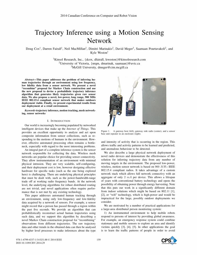
Figure 1. A gateway host (left), gateway sink radio (center), and a sensorbase unit repeater in an enclosure (right).

and intensity of activity that is occurring in the region. This

allows traffic and activity patterns to be learned and predicted,

and anomalous behaviour to be detected.

We also describe a large physical network deployment of

novel radio devices and demonstrate the effectiveness of this

solution for inferring trajectory data from any number of

moving targets in the environment. The proposed low-power,

wireless, motion sensor network is based on 900 MHz IEEE

802.15.4 compliant radios. It takes advantage of a custom

network stack which allows full network connectivy with an

aggregate of only 2 mA per device. This allows a lifespan

of years with conventional battery technology and opens the

possibility of obtaining power through energy harvesting. Note

that this puts our work in a significantly different domain

from indoor solutions which might be based on 802.11 [1],

[2], or “wifi” technology, which is high-power and would be

impractical for the large, possibly outdoor deployments we

consider.

We are motivated by a number of practical applications for

a large-area distributed person monitoring system:

1) An instrumented environment to help mobile robots

respond to persons of interest by providing global awareness.

For example, an emergency response system could combine

stationary and mobile sensors to explore an area and identify

victims quickly [3], [4], [5]. In other applications the goal

is to learn the traffic patterns of people in order to avoid

2014 Canadian Conference on Computer and Robot Vision

978-1-4799-4337-1/14 $31.00 © 2014 IEEE

DOI 10.1109/CRV.2014.29

159

them [6], [7]. Potential uses for this would be a cleaning robot

in a commercial setting or a robot doing warehouse inventory

management. Once the traffic patterns of people are known, a

minimally intrusive route can be planned.

2) A means for energy savings in commercial and residential

buildings through the adaptive use of heating, ventilation,

and air conditioning (HVAC) as well as lighting based on

learned activity patterns. HVAC schedules could be designed

intelligently to minimize energy expenditures during low use

times in specific areas. In the case of lighting, the system could

provide near real time lighting only when needed and could

preemptively light regions based on predicted trajectories [8].

3) A non-intrusive monitoring system for elderly or infirm

individuals. Such a system could allow a better quality of

life for individuals who desire an independent lifestyle but

require monitoring for health and safety reasons. For example,

a detected deviation from the typical daily routine of a senior

in their independent living facility could prompt a visit from

a care-giver [9].

4) A traffic monitoring system for structured outdoor en-

vironments such as gardens, parks, streets and golf courses.

Motion information could be used to identify locations in need

of maintenance, plan landscaping and pathway development,

and plan maintenance schedules.

This paper will continue by discussing related work in

trajectory inference. We will then describe our algorithm as

well as our novel low-power radio sensor network solution.

The experimental results obtained from a large physical de-

ployment are then presented. The final section of this paper

draws conclusions and discusses future work.

II. RELATED WORK

Inferring the trajectory of agents through a sensor equipped

environment shares common aspects with target tracking in

videos. Javed et al. [10] consider recovering agent trajecto-

ries across multiple cameras with non-overlapping fields of

view. Given the use of video cameras, strong appearance

models are available to distinguish different entities. Khan

et al. [11] propose tracking the movements of ants with a

single camera. Due to the lack of a strong appearance model,

they employ a data association inference procedure based

on Rao-Blackwellized Markov Chain Monte Carlo (MCMC).

The inter-camera transition probabilities in [10] are similar to

the inter-zone transition models in this work. In [12], Heath

and Guibas use particle filters for visual tracking of multiple

objects in complex environments. They use overlapping stereo

camera data, which reduces the need for a strong appearance

model or data association procedure.

Trajectory inference has also been treated as a subproblem

in sensor network topology inference [13], [14]. Javed et al.attempt to learn the topology of a video camera network to aid

in multi-target video tracking. Their Parzen window technique

looks at agent velocity and inter-camera travel time.

Ellis, Makris, and Black [15] use temporal correlation

between observations of agent movement to infer the topology

of a video camera network. While their experiments concern

the use of video camera networks, their method does not

require object correlation between cameras.

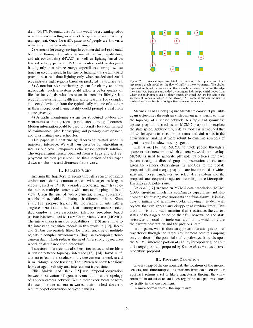
Figure 2. An example simulated environment. The squares and linesrepresent a graph model for the flow of traffic in the environment. The circlesrepresent deployed motion sensors that are able to detect motion on the edgethey intersect. Squares surrounded by hexagons indicate potential nodes fromwhich the environment can be either entered or exited (i.e. are incident to thesource/sink vertex s, which is not shown). All traffic in the environment ismodeled as transiting in a straight line between these nodes.

Marinakis and Dudek [13] use MCMC to construct plausible

agent trajectories through an environment as a means to infer

the topology of a sensor network. A simple and symmetric

update proposal is used as an MCMC proposal to explore

the state space. Additionally, a delay model is introduced that

allows for agents to transition to source and sink nodes in the

environment, making it more robust to dynamic numbers of

agents as well as slow moving agents.

Kim et al. [16] use MCMC to track people through a

sparse camera network in which camera views do not overlap.

MCMC is used to generate plausible trajectories for each

person through a directed graph representation of the area

given the camera observations. In addition to the update

proposal, split and merge proposals are incorporated in which

split and merge candidates are selected at random and the

proposals are accepted or rejected according to the Metropolis-

Hastings probability ratio.

Oh et al. [17] propose an MCMC data association (MCM-

CDA) algorithm which has split/merge capabilities and also

accounts for missing measurements and false alarms. It is also

able to initiate and terminate tracks, allowing it to deal with

objects that can appear and disappear at random times. This

algorithm is multi-scan, meaning that it estimates the current

states of the targets based on their full observation and state

history, as opposed to single-scan algorithms, which only use

the current observation and the previous state.

In this paper, we introduce an approach that attempts to infer

trajectories through the larger environment despite sampling

only a subset of the potential traffic pathways. It builds upon

the MCMC inference portion of [13] by incorporating the split

and merge proposals proposed by Kim et al. as well as a novel

recombine proposal.

III. PROBLEM DEFINITION

Given a map of the environment, the locations of the motion

sensors, and timestamped observations from each sensor, our

approach returns a set of likely trajectories through the envi-

ronment in addition to statistics regarding the patterns taken

by traffic in the environment.

In more formal terms, the inputs are:

160

1) A weighted graph, G = (V,E), embedded in the envi-

ronment. The vertices V = {vi} and edges E = {ei,j}represent a model of intersections and pathways that

are used by traffic in the region. All traffic in the

environment is assumed to occur along the edges of

this graph. The weight wi,j assigned to each edge is

proportional to the geometric distance that is traveled

by traffic between vertices vi and vj .The graph also includes an additional virtual source/sinkvertex s that represents the outside world. Vertices in

V from which traffic can enter and exit the region are

modeled as having an edge incident on the vertex s.2) A model of the detection zones Z = {zi} which repre-

sents the location of the motion sensors with respect to

the environment embedding G. We model each sensor

location as intersecting exactly one edge. Therefore to

identify a sensor location it is only required to specify

the edge and the distance from the head of said edge.

zk = (i, j, wk), represents a sensor whose detection zone

intersects the embedding of edge ei,j , and its distance

from vi is converted to a weight with the same ratio as

wi,j . In other words, 0 ≤ wk ≤ wi,j See Figure 2 for a

pictorial example.

3) A set of observations O = {ot,d,k}, with ot,d,k generated

from the sensor at location zk, with a timestamp t and

a duration d.

4) A model for the velocity of a unique traffic source, the

agent (e.g. a human), in the environment.

Given the inputs described above, the problem we consider

is how to infer a likely set of trajectories Ω = (T1, T2, . . . , TN )that indicate how and where unique agents potentially moved

through the environment. We represent each trajectory Tk ={vi,t}, as an ordered list of visits to vertices at specific times.

Additional statistics about the traffic flowing through the

environment can be determined based on this set of tra-

jectories. For example, a distribution for the transit time

across each edge and the inter-vertex transition probabilities

can be determined. The average number of agents and their

activity level (based on velocity) in various sub regions of the

environment can be determined on a per-time-of-day basis.

IV. TRAJECTORY INFERENCE ALGORITHM

In this section we describe our approach to the trajectory

inference problem described in Section III. The algorithm

works as follows:

1) Given the topological representation G and the agent

velocity model we first determine both an inter-vertextransition matrix A and a model for inter-vertex transi-

tion times D.

2) Given A and D, we then infer an inter-zone transition

matrix A′ and a model for inter-zone transition times

D′. We do this by generating samples of random walks

through G and collecting statistics on these walks.

3) Using A′ and D′ and the observations O, we then

sample a likely instance of the data association K =[ki = agentj ] between each of the observations oi and

potential agents in the environment (agentj , 1 ≤ j ≤

N ). This is done using Markov Chain Monte Carlo

(MCMC). The data association defined by K specifies

a set of inter-zone trajectories Ω′ = {T ′1, T

′2, . . . , T

′N}.

4) Using the set of inter-zone trajectories Ω′ we then infer

a set of inter-vertex trajectories Ω on G. This is done

using Bayesian filtering.

Below we elaborate on each of these steps in more detail.

A. Compute inter-vertex transition and duration models

For the moment, to compute A we make the assumption

that all edges incident on a vertex in G are equally likely;

i.e. the element aij of A has a value inversely proportional to

the degree of vi. Alternatively, this model could be directly

provided to the algorithm if available.

To compute D we use the edge weights (which correspond

to geometric distance) and the agent velocity model to form a

beta distribution. Again, this model could be directly provided

if available. To this we add a simple dwell time model in the

form of a uniform distribution.

B. Compute inter-zone transition and duration models

Given G, A, and D we generate a number of random walks

on G. Each random walk begins with the source/sink node sand ends when a transition returns to s. The statistics obtained

from this set of random walks is then used to fit an inter-

detection-zone transition matrix A′ and duration model D′.Note that given the many potential ways in which traffic could

flow between two detection zones, the duration model D′ is

potentially multi-modal. Therefore we use a mixture model to

represent D′.

C. Infer the agent-to-observation data association

We construct a Markov chain in which each state Kspecifies a data association between the observations and

the agents in the environment. In the single agent case,

the observations O specify a single trajectory through the

edges of the graph instrumented with detection zones. The

algorithm attempts different data associations that break O into

multiple single agent trajectories. Each of these associations

corresponds to a different state in the Markov chain and

is specified with a different observation-to-agent assignment

(observation assignment) vector.

We construct the chain using the Metropolis-Hastings al-

gorithm [18]. From the current state in the Markov Chain

specified by the current observation assignment K, we propose

a transition to a new state using a set of proposals which we

specify in the next section. The new data association as defined

by K ′ is then accepted or rejected based on the following

acceptance probability:

α = min

(1,

p(K ′, O|θ)q(K|K ′)p(K,O|θ)q(K ′|K)

)(1)

where θ = (A′, D′) models the inter-zone transitions,

p(K ′, O|θ) is the likelihood of the model given the observation

set and observation assignment K ′, p(K,O|θ) is the likeli-

hood of the model given the observation set and observation

161

(a) (b) (c) (d)

Figure 3. The proposal strategies used in the MCMC portion of the algorithm: (a) update; (b) split; (c) merge; and (d) recombine. The vertical lines representspecific trajectories and the circles and diamonds represent observations ordered vertically in time. The trajectories to the left of the arrow represent examplesof a state in the Markov chain in which the green circles are observations assigned to one agent and the red diamonds are observations assigned to another.The trajectories to the right of the arrow show examples of how the observations are reassigned by the proposal type. For example, (a) shows to the arrow’sleft two trajectories explained by two sequences of observations, and to the arrow’s right the result of the update proposal reassigning a single observationfrom one trajectory to the other.

assignment K, and finally q(K ′|K) specifies the probability

of proposing state K ′ given state K.

The approach we take here is similar to the MCMC portion

of the algorithm described in prior work by Marinakis and

Dudek [13] and the reader can refer to it for further details.

We have, however, augmented the earlier approach with the

split and merge proposal introduced by Kim et al. in [16] and

have added a novel recombine proposal.

Below, we briefly describe each of the proposals used

in the construction of the Markov chain. Figure 3 gives a

pictorial example of each proposal type and how the proposed

trajectories are affected.

1) Update: This is the symmetric proposal first introduced

in [14]. This reassigns the label associated with a single

observation.

2) Merge and split: This is a pair of proposals introduced

by Kim et al. [16] that allow the chain to consider solutions in

which the observations have been generated by various num-

bers of agents. The two proposals, however, are not symmetric;

i.e. q(K ′|K), the probability of proposing the state K ′ given

K, is not equal to q(K|K ′). These proposal distributions must

be specified in the formulation of the Metropolis-Hastings

algorithm in order to ensure the fair sampling of correct target

distribution. This detail was omitted in [16] and we provide it

here for completeness.

In the merge proposal, the trajectories of two agents selected

uniformly at random are merged to form a single trajectory.

Since this can be done in(|Ω′|

2

)ways where |Ω′| is the current

number of agents, q(K ′|K) is the inverse of this value. In

the split proposal, a random observation is selected uniformly

at random and the containing trajectory is split at that point.

Since this can be done |O| − 1 ways, q(K ′|K) is the inverse

of this value. Here we assume the split and merge proposal

types are considered with the same frequency.

3) Recombine: Here we introduce a recombine proposal in

which the observations associated with two randomly selected

agents are swapped from a specific instance in time. Like the

update proposal, this proposal is also symmetric and allows

for relatively small jumps through the state space.

Figure 4. Spider protocol stack compared to the Open Systems Intercon-nection (OSI) protocol stack model.

D. Infer the trajectories Ω on G

The sampled data association defined by K specifies a set of

inter-zone trajectories Ω′ = {T ′1, T

′2, . . . , T

′N} for N distinct

agents in the environment. Each T ′i specifies a temporally

ordered and timestamped list of motion-sensor-instrumented

edges in G that were assumed to be traversed by agent i.The final step is to infer the larger set of trajectories Ω as

a function of T ′. This is done using a stochastic Bayesian

filtering technique similar to Markov localization techniques

used in robotics, e.g. in [19]. For each consecutive pair of

zones zi, zj in the trajectory T ′ and their inter-detection

duration time δ, we want to infer the path taken in G between

zi and zj . We do this by generating a set of random walks Ron G originating at zi and terminating at either the sink/source

node s or when the walk has reached a vertex with a time that

exceeds δ. Each walk is generated according to the transition

model (A, D) and weighted by it’s likelyhood given the

observation data. Specifically, those walks in which the edge

intersected by zone zj was traversed during the period of

time that include δ are weighted by the likelihood of being

in zone zj at time δ. All other walks in R are pruned from

consideration. A walk is then re-sampled from the remaining

weighted set. The full inferred trajectory T is then generated

by considering each pair of zones in T ′.

V. SYSTEM DETAILS

A. Spider stackIn this section we describe Spider, our network stack. The

Spider stack is a flexible and reliable mesh networking stack

162

suitable for low-cost, low-power, long-distance wireless sensor

networks such as a motion tracking system deployed in a

large store, warehouse, or outdoor environment. It relies on

adaptive mesh routing across multiple frequency bands with

each node having the ability to locate neighbouring nodes

and manage its own time and frequency synchronization. In

that way the Spider stack imposes minimal limitations on

network configuration; allows nodes to enter, leave, or move

in the network at any time; ensures resiliency to changing

environmental conditions; and requires minimal maintenance.

The Spider stack is built on Atmel’s 802.15.4 MAC.1 We

use modified versions of Atmel’s physical and transceiver

abstraction layers, combined into a Hardware Abstraction

Layer (HAL) to provide access to the transceiver and physical

hardware components (e.g. LEDs, switches, timers, and serial

ports). We discard Atmel’s higher layers and scheduler, which

are not suitable for low-power mesh applications, and replace

them with our own stack:

HAL: The Hardware Abstraction Layer provides an API for

basic low-level functionality. It can be used to configure the

transceiver and to perform single-hop transmissions to a partic-

ular network node identified by address and network ID. It also

includes a custom scheduler derived from the microcontroller’s

real-time counter, which runs while the microcontroller is

asleep and which generates the accurate timing needed by

higher layers while minimizing power consumption.

MRM: The Mesh-Ready MAC layer implements a protocol

for synchronizing transmissions between asynchronous nodes

in the mesh network, which allows the network nodes to sleep

99% of the time. It also manages adaptive routing of multi-

hop data between neighbouring nodes and takes care of local

load balancing and spatial redundancy.

Network: The Network layer maintains the network state.

It sends keep-alive messages to neighbours to detect when

a node has lost connectivity, it provides a mechanism for

a node to re-join the mesh, and it implements a message

retry queue to improve data reliability. The network layer

also transmits network diagnostic packets that contain link

statistics, topological information, and debug information.

Spider API: The Spider API implements a serial protocol

for exposing the stack’s functionality to host controllers, e.g. a

sensor node sending data over the mesh network or a gateway

server receiving and processing the incoming data. The API

also implements outbound data flow for dynamic network

configuration and over-the-air programming.

The Spider network allows for three types of device:

Emitters: End devices that collect data and send them toward

the network gateway. Emitters join the network at startup by

listening for beacons sent by sinks and repeaters, but other than

network maintenance they do not listen for incoming data and

as such are extremely low-power devices.

Sinks: Root devices that are hosted by the gateway. Data

packets flow towards sinks. A sink is assumed to be powered

by its host rather than from batteries, so one sink can service a

large network without compromising availability in the name

of power saving. A sink periodically transmits beacons to

1http://www.atmel.ca/tools/IEEE802_15_4MAC.aspx

(a) (b)

Figure 5. Motion sensor components: a) SiFLEX02 900 MHz Radio ona breakout board. b) A motion sensor module.

Figure 6. Motion sensing network architecture.

inform nearby nodes of its presence on the network.

Repeaters: Devices enabling multi-hop transmission by

receiving data packets from emitters and other repeaters,

and re-transmitting them towards a sink. Repeaters need to

spend some time listening for incoming data and transmitting

beacons, so they consume more power over the lifetime of the

network compared to emitters (but less compared to sinks).

B. Hardware

We use a 900 MHz radio board (Figure 5(a)) that includes

an Atmel ATxmega256A3 micro-controller, an AT86RF212

802.15.4 radio, and a custom 24 dBm power amplifier. We

use a custom board for breaking out the radio’s surface-mount

pad hardware interface. The breakout board provides JTAG

programming, SPI, I2C, UART, GPIO (including ADC and

DAC pins), and LED interfaces.

We power the radio from two AA batteries. Overall power

consumption depends primarily on three variables: packet size,

transmission rate, and network parameters. With its 24 dBmpower amplifier enabled, empirical measurements show that

the radio draws about 250 mA while it is transmitting. We

transmit data using the 802.15.4 specification’s 250 kbpsOQPSK configuration; thus a single 5-byte packet consumes

approximately 100 μJ of energy. The Spider stack supports

packets of up to 112 bytes (approximately 2.5 mJ).

The network parameters—beacon length, receive slot

length, number of receive slots, etc.—and transmission rate

also affect total power consumption. A transmission rate of one

5-byte packet every 80 seconds combined with “fast” network

parameters results in a long-term average current draw of about

2 mA. A transmission rate of one packet every 10 minutes

combined with “low-power” network parameters results in a

long-term average current draw of about 120 μA.

163

Figure 7. Example of a field trial deployment site. Devices were placed ingroups of five throughout the site in simple glass enclosures.

C. Motion sensing network

Our motion sensing network is built around a base unit that

houses a radio and power source. It exposes four sensor ports,

and can be deployed anywhere without the need for wires.

The sensor modules that plug into the ports (Figure 5(b)) have

Panasonic passive infrared (PaPIR) sensors broken out to four

pins: positive voltage, ground, output, and sensor detect. The

PaPIR output is an open drain configuration that oscillates

between open and closed while the sensor is detecting motion

and remains open when the sensor does not detect motion.

The sensor detect pin indicates to the base unit that a sensor

port has a sensor module connected to it.

The motion sensing application runs on top of the Spider

stack on a base unit microcontroller. Over time it builds a

message comprised of 16 bits for each sensor that is connected

to the main board. Each bit represents whether the sensor

detected motion during a 5-second interval. When a sensor

detects motion it wakes up the microcontroller, which stores

the detection bit. Any further detection by that sensor is

ignored until the 5-second interval expires, at which point the

microcontroller once again starts listening for detections on

all sensors. Every 80 seconds the 16-bit detection histories

are transmitted over the Spider network.

Once the data are obtained by the gateway device, they are

back hauled via a message queue to a database residing on a

server. A browser based interface provides network diagnostics

and the motion sensing data are accessed via an API by

consumer applications (Figure 6).

For our motion sensing application we affix two sensors to

each base unit’s enclosure (as shown to the right of Figure 1).

Sensors can be placed freely and wired to base units, but for

the purpose of this experiment we mount the sensors to adja-

cent walls of the enclosure. In that way sensor directionality

for each base unit is easily modeled as orthogonal vectors,

with one sensor directed 90◦ clockwise from the other sensor

(see Figure 11(a)).

VI. EXPERIMENTAL RESULTS

A. Spider stack

Through outdoor field deployments we have verified the

low power usage and self-healing nature of the Spider network

stack. In one experiment we deployed 50 devices on a densely

treed 6 hectare test site. We placed devices in weatherproof

Figure 8. Google Earth image showing the ten deployment sites (markers Athrough J) and the location of the sink gateway (marker labeled Sink). Whitelines depict typical routing paths.

enclosures and deployed them in groups of five in ten different

locations spread out evenly over the site (Figure 7). We used a

simple test application that sent voltage readings and dummy

sensor data every four seconds.

We analysed logs from a 48 hour period for network

health purposes. Approximately one quarter to one third of

the devices selected routes that allowed them to communicate

directly to the gateway device during this time period. The

remainder used multi-hop routes typically two or three hops in

length (Figure 8). Occasionally we observed four hop routes.

We computed average packet latency to be approximately

125 ms.

B. Investigation of trajectory inference through simulation

Through simulation we have verified the basic correctness of

the trajectory inference approach. The performance, however,

is affected by a number of factors including the accuracy

of the model, the ratio of instrumented to non-instrumented

edges, the number of agents in the environment, the entropy

associated with the edge transition time model and transition

matrix, the ability to constrain the environment to a graph

model, and finally the topology and size of environment.

In Figure 9 we show an example of how the number of

instrumented edges influences the accuracy of the approach. In

this experiment we generated data based on a transition matrix

that differs from the one assumed by the algorithm. Figure 9(a)

displays the relative edge transit frequencies based on a

random walk using the assumed—but incorrect—transition

matrix. The well-instrumented deployment shown in 9(c)

accurately infers the actual edge transit frequencies, while the

deployment with only four sensors shown in Figure 9(b) infers

a result that is biased by the assumed transition matrix.

164

(a) (b) (c)

Figure 9. A set of simulated environment graphs in which the squares represent nodes and the circles represent deployed motion sensors that are ableto detect motion on the edge they intersect. The relative edge traversal frequencies are represented by edge width for the various simulated scenarios: a) atrajectory generated using the incorrect transition matrix A assumed by the algorithm; b) a trajectory generated using B and inferred using four deployedsensors; c) a trajectory generated using the actual transition matrix B and accurately inferred using six deployed sensors.

(a)

(b)

Figure 10. Example of the progression of the trajectory inference algorithmas a function of the number of MCMC proposals on the simulated environmentshown in Figure 2. a) The probability of the inferred solutions increases andeventually levels off at the probability of the true solution (shown as a dottedline). b) The corresponding inferred number of agents in the environment withthe true number shown as a dotted line.

Our approach is able to accurately estimate the number

of agents in the environment as long as the ratio of agents

to edges in the environment is relatively low. Consider the

simulated environment shown in Figure 2. Figure 10 shows the

progression of solution likelihoods and the associated number

of agents as a function of the Markov chain proposals.

Note that in this scenario, the chain mixes well and con-

verges to a solution among those with the same likelihood

as the true solution. If the ratio of agents to edges in the

environment is too high, however, the problem becomes under-

constrained and the algorithm is able to find inaccurate solu-

tions that have the same or higher likelihood than the actual

solution. This is illustrative of the challenging nature of this

problem.

C. Motion sensing network deployment

To test our approach, we deployed the motion sensing

network in a retail space (Figure 11(a)). We used a simplified

(a)

(b)

Figure 11. Motion sensing network deployment: a) Floor plan of thedeployment area. White vectors represent the placement and direction of themotion sensor modules. b) Simplified model where squares represent nodes inthe environment. Squares surrounded by hexagons indicated potential nodesfrom which the environment can be either entered or exited. Circles representdeployed motion sensors. The line widths are proportional to the inferredfrequency of edge transits.

graphical model of the environment and sensor deployment to

model the traffic in the store. The raw data consisted of over

five thousand observations from the ten sensors. Processing

using the trajectory inference algorithm took approximately 10

hours on an Intel Core i7-based computer with 8 GB of RAM.

The data were pre-processed to debounce multiple consecutive

detections and then post-processed to remove low probability

trajectories.

We selected a full business day (a Saturday) for analysis

and ran our trajectory inference algorithm on the resulting

data. Figure 11(b) shows a simplified graphical model of the

store in which the edge widths are proportional to the inferred

number of edge transits in the region. Figure 12 shows the

inferred number of agents in the environment. Note that these

results are based on a likely trajectory set sampled by the

Markov chain. Other samples of likely trajectory sets provide

slightly different details but show the same general trends. The

165

Figure 12. Plot showing the number of inferred agents in the environment as a function of offset in minutes from 7:00 AM.

results obtained are consistent with our expectations of how

the traffic might typically flow through the area.

VII. CONCLUSIONS AND FUTURE WORK

We have proposed a novel, low-power, wireless motion

sensor network for inferring trajectory data. The system uses

current wireless technology to sense activity, and an MCMC-

based algorithm to process the observations. We have given

a novel problem formulation, described our approach, and

presented promising results from a real world deployment.

In future work we will consider providing confidence met-

rics on the inter-sample variance of a set of solutions returned

from the Markov chain. Additionally, we will consider using

the Expectation Maximization algorithm to refine our initial

model of the environment. Specifically, it should be possible

to learn more accurate models of the transition matrix and

temporal distributions in an online fashion. An additional

interesting problem is the question of where to position the

motion sensing zones so that the trajectories on G can be

inferred with the greatest accuracy. This is related to the work

of Ali et al. in [20].

ACKNOWLEDGEMENT

We would like to thank Colin How, Christopher Shannon,

and Rob King for their technical help and stimulating conver-

sation regarding the motion sensor network; Jason Dunlop and

Sean Dunlop for allowing us to deploy the prototype in their

retail store; Dan Winner, Scott Craig, Tubego Phamphang,

Catherine Gamroth, and Nathan McLean for their technical

help on the network stack; and finally Michelle Theberge for

her administrative assistance. We acknowledge the Industrial

Research Assistance Program of Canada for their funding.

REFERENCES

[1] J. T. Adams, “An introduction to ieee std 802.15. 4,” in AerospaceConference, 2006 IEEE. IEEE, 2006, pp. 8–pp.

[2] B. P. Crow, I. Widjaja, L. Kim, and P. T. Sakai, “Ieee 802.11 wirelesslocal area networks,” Communications Magazine, IEEE, vol. 35, no. 9,pp. 116–126, 1997.

[3] E. Ferranti, N. Trigoni, and M. Levene, “Rapid exploration of unknownareas through dynamic deployment of mobile and stationary sensornodes,” Autonomous Agents and Multi-Agent Systems, vol. 19, no. 2,pp. 210–243, 2009.

[4] Q. Zhang, G. Sobelman, and T. He, “Gradient-driven target acquisitionin mobile wireless sensor networks,” in Mobile Ad-hoc and SensorNetworks. Springer, 2006, pp. 365–376.

[5] M. A. Batalin, G. S. Sukhatme, and M. Hattig, “Mobile robot navigationusing a sensor network,” in Robotics and Automation, 2004. Proceed-ings. ICRA’04. 2004 IEEE International Conference on, vol. 1. IEEE,2004, pp. 636–641.

[6] M. Bennewitz, W. Burgard, G. Cielniak, and S. Thrun, “Learningmotion patterns of people for compliant robot motion,” The InternationalJournal of Robotics Research, vol. 24, no. 1, pp. 31–48, 2005.

[7] A. M. Eames, “Enabling path planning and threat avoidance withwireless sensor networks,” Ph.D. dissertation, Citeseer, 2005.

[8] I. Khan, N. Javaid, M. Ullah, A. Mahmood, and M. Farooq, “A surveyof home energy management systems in future smart grid communica-tions,” arXiv preprint arXiv:1307.7057, 2013.

[9] F. Viani, F. Robol, A. Polo, P. Rocca, G. Oliveri, and A. Massa, “Wirelessarchitectures for heterogeneous sensing in smart home applications:Concepts and real implementation,” 2013.

[10] O. Javed, Z. Rasheed, K. ShaïnAque, and M. Shah, “Tracking acrossmultiple cameras with disjoint views,” in Proc. of International Confer-ence on Computer Vision, 2003.

[11] Z. Khan, T. Balch, and F. Dellaert, “Mcmc data association and sparsefactorization updating for real time multitarget tracking with mergedand multiple measurements,” IEEE Transactions on Pattern Analysisand Machine Intelligence, vol. 28, no. 12, pp. 1960 – 1972, December2006.

[12] K. Heath and L. Guibas, “Multi-person tracking from sparse 3d trajecto-ries in a camera sensor network,” in Distributed Smart Cameras, 2008.ICDSC 2008. Second ACM/IEEE International Conference on. IEEE,2008, pp. 1–9.

[13] D. Marinakis and G. Dudek, “Occam’s razor applied to network topologyinference,” Robotics, IEEE Transactions on, vol. 24, no. 2, pp. 293–306,2008.

[14] D. Marinakis, G. Dudek, and D. Fleet, “Learning sensor networktopology through monte carlo expectation maximization,” in IEEE Intl.Conf. on Robotics and Automation, Barcelona, Spain, April 2005, pp.4581–4587.

[15] D. Makris, T. Ellis, and J. Black, “Bridging the gaps between cameras,”in IEEE Conference on Computer Vision and Pattern Recognition CVPR2004, vol. 2, Washington DC, June 2004, pp. 205–210.

[16] H. Kim, J. Romberg, and W. Wolf, “Multi-camera tracking on a graphusing markov chain monte carlo,” in Distributed Smart Cameras, 2009.ICDSC 2009. Third ACM/IEEE International Conference on. IEEE,2009, pp. 1–8.

[17] S. Oh, S. Russell, and S. Sastry, “Markov chain monte carlo dataassociation for general multiple-target tracking problems,” in Decisionand Control, 2004. CDC. 43rd IEEE Conference on, vol. 1. IEEE,2004, pp. 735–742.

[18] W. Hastings, “Monte carlo sampling methods using markov chains andtheir applications,” Biometrika, vol. 57, pp. 97–109, 1970.

[19] S. Thrun, D. Fox, and W. Burgard, “A probabilistic approach to con-current mapping and localization for mobile robots,” Machine Learningand Autonomous Robots (joint issue), 1998.

[20] S. Ali, K. Weston, D. Marinakis, and K. Wu, “Intelligent meter place-ment for power quality estimation in smart grid,” in Smart Grid Commu-nications (SmartGridComm), 2013 IEEE International Conference on.IEEE, 2013, pp. 546–551.

166