Transaction Costs and the Duration of

Contracts

Alexander MacKay

Working Paper 18-058

Working Paper 18-058

Copyright © 2017 by Alexander MacKay

Working papers are in draft form. This working paper is distributed for purposes of comment and discussion only. It may

not be reproduced without permission of the copyright holder. Copies of working papers are available from the author.

Transaction Costs and the Duration of

Contracts

Alexander MacKay Harvard Business School

Transaction Costs and the Duration of Contracts∗

Alexander MacKayHarvard University†

December 29, 2017

Abstract

The duration of a vertical relationship depends on two types of costs: (i) the trans-action costs of re-selecting a supplier and (ii) the cost of being matched to an inefficientsupplier when the relationship lasts too long. For commodified goods and services, thistradeoff can be the primary determinant of the duration of supply contracts. I develop amodel of optimal contract duration that captures this tradeoff, and I provide conditionsthat identify underlying costs. Latent transaction costs are identified even when the ex-act supplier selection mechanism is unknown. I estimate the model using federal supplycontracts and find that transaction costs are a significant portion of total buyer costs. Iuse the structural model to estimate the value of the right to determine duration to thebuyer, compared to a standard duration. Finally, a counterfactual analysis illustrateswhy quantifying transaction costs is important for the accurate analysis of welfare.

∗An earlier version of this paper circulated with the title "The Structure of Costs and the Duration of Sup-ply Relationships." This version reflects an expanded data collection effort and a larger dataset. I am especiallygrateful for the helpful comments and suggestions of Ali Hortaçsu, Brent Hickman, Casey Mulligan, Chad Syver-son, and Stephane Bonhomme. I also thank seminar and conference participants at the University of Chicago,the CEPR-JIE Conference, the Econometric Society World Congress, Northwestern (Kellogg), Harvard BusinessSchool, Carnegie Mellon, UCLA (Anderson), Rice, and the International Industrial Organization Conference.†Harvard University, Harvard Business School. Email: amackay@hbs.edu.

1 IntroductionWhen buyers transact with sellers, they select not only who but also how long. The duration

of buyer-seller agreements determines transaction frequency and is fundamental to vertical

relationships. As Oliver Williamson wrote, "the three critical dimensions for characterizing

transactions are (1) uncertainty, (2) the frequency with which transactions recur, and (3) the

degree to which durable transaction-specific investments are incurred" (Williamson, 1979).

Though much attention in the economics literature has been given to relationship-specific

investments and transactions under uncertainty, the frequency dimension has received com-

paratively little attention, especially in the absence of the other two forces. Even in simple

environments, frequency is inherently linked to prices and transaction costs.

Consider supply contracts for commodified goods and services, such as raw materials,

electricity, paper products, accounting services, and office cleaning. These contracts are

perhaps the most common form of vertical agreement, and they are typically characterized

by fixed-price, fixed-duration terms.1 In these settings, relationship-specific investments

are small, and the costs of uncertainty are minimized through the fixed-price terms of the

contract. The simple nature of the contracts also indicates that the ex post alignment of

incentives may be of lesser concern. The observation that commodified products are sold

on contracts, and not solely in spot markets,2 suggests that the transaction costs of selecting

a supplier and determining price are meaningful.3 Through equilibrium contracts, which

lie between spot markets and vertical integration, these costs mediate how prices respond

to changes in the economic environment.

In the absence of concerns about uncertainty and relationship-specific investments, the

optimal duration depends on transaction costs, variation in supply costs, and competition.

Consider a buyer with unit demand in an environment with perfect information and id-

iosyncratic variation in supply costs over time.4 With no transaction costs, spot markets are

efficient, as the buyer can select the lowest-cost supplier in each period. At another extreme,

with no supply-side competition, a permanent contract (integration) will be efficient, as the

monopolistic seller will be the lowest-cost supplier in each period. When selecting among

multiple sellers, a multi-period contract will generally not select the lowest-cost supplier in

each period, resulting in increased supply costs. The equilibrium contract therefore reflects1In their seminal NBER survey, Stigler and Kindahl (1970) found that about half of the commodities in their

sample were purchased with fixed-term contracts. A more recent comprehensive survey has not been con-ducted (and would be welcome). Fixed-price contracts constitute the vast majority of U.S. federal governmentcontracts, and, anecdotally, remain predominant in the private sector.

2Services and products may also have a quality dimension, though for many commodities suppliers competefor the lowest price that meets a minimum quality or particular specifications.

3Transaction costs may include search, contracting, negotiation, and switching costs.4The lowest-cost supplier may change over time due to capacity constraints, heterogeneity in outside options,

innovation, and other factors.

1

both the degree of competition and underlying costs.

In this paper, I present a model of contract duration where a buyer selects a seller from

an imperfectly competitive market. The buyer sets the non-price terms of the contract

(duration), and the price is determined by a competitive game. In equilibrium, the buyer

chooses duration to minimize expected buyer costs, which include both the price paid to the

supplier and the (amortized) transaction costs faced by the buyer. These features reflect a

typical real-world contracting problem. Indeed, the tradeoff between reducing transaction

costs on the one hand and more frequently re-selecting a supplier on the other is intuitive.5

This paper explores this tradeoff and its empirical implications through a simple theo-

retical model, a structural empirical model, and an empirical application. The structural

model, wherein contract duration is determined endogenously, is one of the main contribu-

tions of this paper. The model allows one to address the following questions: How large are

transaction costs? And, further, how valuable are duration-setting rights in a transaction?

One of the challenges in evaluating the impact of transaction costs is that they are often

unobserved or difficult to quantify. The empirical strategy of this paper, based on the ob-

servation that the equilibrium duration reflects the underlying cost structure, provides for

the identification of latent transaction costs. I estimate the model in the context of building

cleaning contracts for the U.S. federal government, which provide an ideal environment to

study the duration problem for a commodified product.6 I find that transaction costs are

large and economically meaningful in this setting, comprising 10.8 percent of total buyer

costs. Counterfactual analysis indicates that the ability of the buyer to determine duration is

valuable, relative to a poorly-chosen standard duration, but also that an intelligently-chosen

standard would be cost effective if it induced moderate declines in transaction costs.

To build intuition, I explore the tradeoff between transaction costs and supply costs us-

ing a simple example. In Section 2, I present a two-period model where the buyer picks

either two one-period contracts or a single two-period contract. The simple model provides

some intuition about the tradeoff, the relation to underlying supply costs, and the degree of

competition. For example, the model generates the intuitive prediction that higher autocor-

relation in supply costs leads to longer contracts. Less intuitive is the result that the optimal

duration is U-shaped in the number of suppliers competing for the contract. With low lev-

els of competition, long-term contracts are optimal, as the benefit of re-selecting a supplier

is small. This benefit increases as competition increases, resulting in short-term contracts

at moderate levels of competition. When competition is intense, the buyer can secure a

low-enough price for an extended period that long-term contracts are once again optimal.5This tradeoff coincides with how several procurement and purchasing personnel described the duration

decision to the author. Re-selecting a supplier may include re-negotiation with an incumbent supplier.6Building cleaning services are one of the most contracted-for products for the federal government. They

are relatively homogeneous, and cost factors (such as square footage) are readily quantifiable.

2

Figure 1: Model Summary

Price

Contract Duration

Number of Bids

TransactionCosts

ContractCharacteristics

EntryConditions

Notes: The figure summarizes the causal assumptions embedded in the empirical model.The three sets of variables on the left: entry conditions, contract characteristics, andtransaction costs, are taken as given. Price, number of bids, and contract duration arejointly determined in the model. Arrows indicate the direction of causality.

Though I focus on the buyer-optimal contract, the efficient contract has similar qualitative

predictions. At the end of the section, I discuss how the model and its predictions can be

translated to a bundling problem.

As the simple model demonstrates, the optimal duration policy is inherently empirical.

In Section 3, I develop an empirical model of buyer-seller transactions with endogenous

duration. The buyer has inelastic demand for a single good in each period. The model

consists of three stages: (1) the buyer sets the duration of the contract, (2) suppliers decide

whether to participate in a supplier selection mechanism, and (3) the supplier and the price

are determined by the mechanism. I present assumptions sufficient for the identification

of transaction costs, which is possible even without additional structure on the third-stage

game.7 The empirical strategy is sequential and separate. First, estimate the final two

stages of the model, and then, in an independent step, estimate transaction costs. Once

key components of the model are identified, transaction costs may be recovered from the

optimality conditions of the buyer’s duration decision. Figure 1 summarizes the causal

assumptions embedded in the model.

I then consider nonparametric identification when the supplier selection mechanism is

an auction, which parallels the empirical setting. Even with unobserved heterogeneity, the

additional structure allows for the identification of seller surplus and (partial) identification

of the joint distribution of costs without information on other bids or a reserve price. This, in7Thus, this result may be useful for analyzing contracts where the underlying selection process may be

obscure, such as contract negotiations that occur privately.

3

turn, provides for identification of the efficient contract and the calculation of welfare under

counterfactuals. Like many previous auction models, entry is endogenous and depends on

market conditions and contract characteristics. One feature that distinguishes this model is

the endogenous determination of duration as a third outcome.

Though a central focus of this paper is the choice of duration, the auction identifica-

tion results for multiplicative unobserved heterogeneity and (a particular form of) selective

entry apply even when no duration decision is present. This arises directly from the sequen-

tial and separate steps described above. The identification results are complementary to the

work of Krasnokutskaya (2011) and Aradillas-López et al. (2013), among others, and make

use of data that is more broadly available. Further, when entry is exogenous, I show that the

distribution of private costs and unobserved heterogeneity is identified through variation in

the number of bidders alone.8 Intuitively, variation in the number of bids shifts the distri-

bution of the private component in a known way, while the distribution of auction-specific

heterogeneity is unaffected. Thus, in settings that may be motivated by the independent

private values assumption, it is also possible to estimate a conditional independent private

values model with unobserved heterogeneity. Researchers who wish to apply auction tech-

niques to transaction price data may use this result to test for and quantify the presence of

unobserved heterogeneity.

In Section 4, I present the empirical context for the application of the paper. From

multiple sources of data, including contract documents, I have constructed a unique dataset

for 1,046 contracts for building cleaning services. The market for cleaning services is a

nice setting to examine the tradeoff of this paper as the product is commodified, key cost

characteristics (such as square footage) are quantifiable, and demand is inelastic. It is

an established market with relatively stable supply-side conditions.9 Transaction costs are

meaningful, as a competitive solicitation entails the labor costs of contracting officers as

well as the costs of background checks.

The buyer in my setting is the U.S. federal government. The set of government contracts

in my data are special, as the government is required, by regulation, to choose the low-price

offer among qualified bidders at the expiration of the previous contract. Thus, the govern-

ment setting provides a close approximation to the theoretical auction model.10 Consistent

with the model, duration is determined ex ante by the local government agency.11

8Previous approaches relied on observing either multiple bids per auction or a reservation price.9Ex post incentive problems, which are a large focus of the contract literature, are not a first-order concern.

Performance is observable, contracts are rarely canceled, and the suppliers in this market are generally well-established firms.

10In other settings, buyers may have other means to secure a seller, such as a direct negotiation with theincumbent supplier. This would complicate the model.

11Additionally, variation in transaction costs for the contracts in my sample may reflect variation in transac-tion costs for a wider set of products, as the same employees handled a broad portfolio of contracts.

4

Next, I take a parameterized version of the structural model to the data. In the first

stage, I find that supply costs are increasing with the duration of the contract, which is

consistent with the equilibrium of the duration-setting model when transaction costs are

present. I find that transaction costs are relative large in this setting, comprising 10.8 per-

cent of total buyer costs. Transaction costs are highest for the most complex facilities, such

as medical centers and airports, and lowest for offices. Of the government agencies, I find

that Homeland Security has the highest median transaction cost, whereas the Department

of Defense, who issues the most contracts and has many simple office buildings, has the

lowest. As a verification test, I also find that the estimated transaction costs are positively

correlated with the number of words in the contract and the amount of related expendi-

tures by the contracting agency in the same location, which aligns with our intuition. These

results are presented in Section 5.

After quantifying the magnitude of transaction costs, I consider the impact of flexible

contract terms in Section 6. Flexible terms allow the buyer to optimize contract by contract.

To calculate the value to the buyer, I consider an alternative policy where all contracts are

issued with a standard duration. Standard terms could be costly: issuing one-year contracts

for the data in my sample would increase total costs by 36 percent, as the total burden of

transaction costs would rise sharply. Of the full-year durations, the four-year standard term

has the lowest impact, increasing total costs by 1.4 percent. We might expect standardiza-

tion to reduce transaction costs, e.g. through reduced effort from the buyer to determine

the optimal duration. I find that relatively modest declines in transaction cost (9.3 percent)

would offset the costs of moving away from optimal contract-specific durations. Thus, a

poorly chosen standard could substantially increase costs, but an informed standard may

be cost effective with moderate reductions in transaction costs.

As a second counterfactual, I consider the impact of endogenous duration and transac-

tion cost on the estimation of welfare effects. Relative to a structural model that take du-

ration as exogenous, the estimated model allows buyers to adjust on an additional margin

(duration) in response to changes to the state, improving buyer surplus relative to environ-

ment in which they are passive. I then compare the estimated effects from the structural

model to a difference-in-differences strategy that measures the change in prices after a pol-

icy that affects transaction costs. The price changes capture only 63 percent of the change

in total costs, implying that a difference-in-differences estimate would substantially under-

estimate the welfare effects compared to a model that explicitly accounted for transaction

costs. As we expect that many policy changes would affect transaction costs, this analysis

suggests that it would be important to take such costs into account.

5

Related Literature

There is a rich empirical literature on the determinants of vertical integration. For a sum-

mary, see Lafontaine and Slade (2007). Vertical contracts in this literature have been iden-

tified as "almost integration," somewhere between arms-length transactions and vertical

integration. This paper adds to this literature by considering the duration aspect of vertical

contracts. This dimension allows firms to choose along an integration continuum, rather

than a binary make-or-buy decision. Factors that lead to longer contracts should also in-

crease the propensity to vertically integrate, as noted by Coase (1960), so the predictions

from the theoretical section of this paper also apply to the integration decision.

The essential connection between transaction costs and contract duration (or vertical

integration) was identified at least as early as Coase (1937).12 Economists studying the

effect of transaction costs on vertical relationships have primarily pursued the testable im-

plications of these costs, rather than their direct estimation.13 Thus, a central contribution

of this paper is a structural empirical model that allows for the direct estimation of these

costs.14 Likewise, the empirical literature on contract duration has also focused on testable

implications, so the structural modeling of duration as an outcome is also a contribution.

To the best of the author’s knowledge, this is the first paper to focus on a general ex

ante cost of longer contracts, which arises from an inefficient supplier match over the du-

ration. The previous literature on contract duration has focused on ex post coordination

problems, primarily through costly renegotiation (Gray, 1978; Masten and Crocker, 1985)

and relationship-specific investments (Joskow, 1987). For clarity, I abstract away from ex

post incentive problems, including risk sharing, principal-agent relationships, the holdup

problem, and incomplete contracting.15 For many commodities, a first-order concern is not

the proper alignment of buyer and seller incentives, but rather that buyers and sellers are

efficiently matched. I am also able to test for and abstract away from an incumbency ad-

vantage, which is a often a concern in settings with repeated contracts (see, e.g. Greenstein

(1993)). My work is complementary to models with these features.

The tradeoff in this paper between transaction costs and price is closely related to the

models of contract duration of Dye (1985) and Gray (1978), who take the stochastic price

process as given. The innovation of this paper is to use tools of industrial organization to

model primitives of the price process and explore its implications. The effect of transac-

tion costs on welfare has primarily been addressed in terms of their impact on equilibrium12Coase wrote: “if one contract is made, instead of several shorter ones, then certain costs of making each

contract will be avoided.”13For examples of the testable implications approach, see Monteverde and Teece (1982), who consider prox-

ies for asset specificity, and Walker and Weber (1984), who include proxies for uncertainty.14Conceptually related is recent work by Atalay et al. (2017), who construct a measurement of external

transaction costs by examining input flows between integrated and non-integrated firms across sectors.15For these features, see, e.g. Holmstrom (1983), Guriev and Kvasov (2005), and Rey and Salanie (1990).

6

prices.16 In markets with vertical contracts, transaction costs may be a sizable portion of

total costs and should be accounted for in addition to any price effects.17

There is a parallel literature on switching costs in consumer markets, which is a different

economic environment from the one analyzed here. A key feature of consumer markets is

an inability to contract on future prices, leading to models that weigh an “investing” effect

versus a “harvesting” effect (Farrell and Klemperer, 2007).18 When buyers and sellers agree

on future prices, as in this paper, these effects are competed away. Further, switching costs

in previous empirical studies can be inferred from posted prices,19 whereas contract prices

are idiosyncratic to the buyer-seller match. Finally, the switching costs literature tends take

supply costs as fixed (see, for example, Beggs and Klemperer (1992)), whereas variation in

supply costs is a key factor in the decision to switch suppliers in my setting.

My contribution to the auction identification literature is most closely related to Kras-

nokutskaya (2011), who solves the problem of disentangling private costs from auction-

specific heterogeneity by relying on two bids per auction. Concurrent work by Quint (2015)

shows how variation in the number of bidders identifies a model with additively separable

unobserved heterogeneity, in contrast to the multiplicative structure examined here. Other

authors have developed results for somewhat more general settings, by relying on three

bids per auction (Hu et al., 2013) or an observable reserve price in addition to the win-

ning bid (Roberts, 2013). Aradillas-López et al. (2013) exploit variation in the number

bids for second-price auctions, though the identification results of their paper are limited

to constructing bounds on surplus. In this paper, I demonstrate point identification of sur-

plus for both first-price and second-price auctions and partial identification of the full joint

distribution of costs.

This model of this paper is equivalent to a simultaneous bundling problem, where the

contract bundles demand over time. Work on bundling by Zhou (2017) and Palfrey (1983)

share some insights with this paper and provide the most closely related analogs. Compared

to their analysis, I allow for intermediate degrees of bundling and introduce transaction

costs. Salinger (1995) and Bakos and Brynjolfsson (1999) note that bundling affects prices

by reducing the variance of average valuations. In this paper, I demonstrate that the smaller

variance induced by bundling reduces total surplus when there are no transaction costs.

Cantillon and Pesendorfer (2006) share this insight in their analysis of combination bidding

for multi-unit auctions.16See Klemperer (1995).17Carlton and Keating (2015) emphasize the role of transaction costs in welfare analysis when the affected

variable is not simply the price level, through the effect on a firm’s ability to implement nonlinear pricing.18For recent papers on this subject, see Cabral (2016) and Rhodes (2014).19See, for example, Dubé et al. (2009) for orange juice and margarine or Elzinga and Mills (1998) for

wholesale cigarettes. The wholesale market in the analysis of Elzinga and Mills (1998) mirrors a consumermarket in that pricing, though nonlinear, is uniformly applied.

7

2 A Simple ModelIn this section, I develop a simple model to illustrate how competition, supply costs, and

transaction costs interact to determine the duration of contracts. I focus on the buyer-

optimal contract, as it reflects the theoretical outcome for the empirical setting of this paper.

The qualitative predictions developed for the buyer-optimal contract will also pertain to the

efficient contract.20 I defer a discussion of efficiency to the end of this section.

Suppose that a risk-neutral buyer is seeking the supply of a good for two periods. There

are N symmetric suppliers in the market, and the set of suppliers stays the same across

both periods. The buyer can issue either a single two-period contract or sequential single-

period contracts. The transaction cost for each contract is δ, which captures search and

information costs, as well as a complementarity of supplying for two periods.

The game proceeds in three steps. First, the buyer selects a duration of either one or two

periods. Second, suppliers realize cost draws for both periods. Third, suppliers participate

in an auction for each contract, i.e. an efficient mechanism.21

The per-period cost to each supplier is the random variable c. When the buyer issues

single-period contracts, the per-period cost of the winning supplier is c1:N , which is the

minimum of N draws of c. When the buyer issues a two-period contract, the average per-

period costs for each supplier is average of two draws, c = c1 + c2, and the cost to the

winning supplier is c1:N .

Remark 1. As long as the per-period costs c are not perfectly correlated across periods, c 6= c

and V ar(c) < V ar(c).

Thus, the buyer changes the effective cost structure faced by suppliers when changing

the contract duration. When the distribution of supply costs is stable over time, this serves

to reduce the variance of cost draws. The cost of a longer contract is that the low-cost

supplier may not be selected in each period. In the absence of transaction costs, short-term

contracts would be optimal.

If we further assume that the buyer is risk-neutral, symmetry in this setting generates the

standard auction result that the expected winning bid is equal to the second-order statistic

from the cost draws. Thus, the buyer-optimal contract solves

min{2E[c2:N ] + 2δ︸ ︷︷ ︸short-term

, 2E[c2:N ] + δ︸ ︷︷ ︸long-term

}

20Intuitively, the predictions depend on the covariance structure and the properties of order statistics. Theexpected cost and the expected price in this simple setting are the first-order and second-order statistics, andthus display similar properties when the number of draws is greater than three.

21In this simple model, suppliers have perfect foresight about future costs. A more general setup with im-perfect information shares the same qualitative features of this model, though there is an additional ex postinefficiency arising from imperfect information.

8

The buyer will pick the long-term contract if the increase in expected supply costs is less

than the reduction in (amortized) transaction costs: E[c2:N ]− E[c2:N ] < δ2 .

Remark 2. Higher marginal costs lead to shorter contracts, and higher transaction costs lead

to longer contracts.

From this simple decision rule and the properties of order statistics, we obtain a set of

comparative statics or predictions. For simplicity of exposition, the predictions are provided

with a brief discussion and illustrated with a numerical example. For further details, see

the Appendix.

Prediction 1 The optimal duration is increasing with autocorrelation in supply costs.

This first prediction is intuitive. As the autocorrelation in marginal costs increases, there

is less of a benefit from selecting the low-cost supplier in each period, and longer-term

contracts are preferred.

Prediction 2 The optimal duration is decreasing in the variance of costs across suppliers,

provided there is sufficient competition (N > 3).

Prediction 2’ When costs are bounded from below, the optimal duration is U-shaped in the

variance in costs, provided there is sufficient competition (N > 3).

From a starting point of zero variance across suppliers, increasing the variance of marginal

costs leads to shorter contracts, as there is more to gain from selecting the low-cost sup-

plier in each period. This holds for the buyer-optimal contract as long as there are more

than three suppliers, in which case the expected second-order statistic falls below the me-

dian.22 When costs are bounded from below, eventually both E[c2:N ] and E[c2:N ] approach

zero, and the cost of longer duration falls with respect to transaction costs. After a certain

threshold, contract duration increases.

Prediction 3 When costs are bounded from below, the number of suppliers has an inverse

U-shape effect on the marginal cost of longer contracts. Therefore, duration may be

decreasing, increasing, or U-shaped with N .

As this simple model illustrates, an increase in the intensity of competition, i.e., the num-

ber of suppliers, has an ambiguous effect on equilibrium contract duration, depending on

underlying market conditions and parameters. For low levels of competition, the benefit

of switching suppliers is low, and long-term contracts are preferred. At moderate levels of

competition, there is an increased benefit of switching among suppliers more frequently.22For the efficient contract, this prediction holds when there are two or more suppliers.

9

When competition is intense, the expected costs of both long-term and short-term contracts

approach the lower bound of costs, and therefore long-term contracts, which minimize

transaction costs, are optimal.

2.1 A Numerical Example

To illustrate the above predictions, I present a simple case in which per-period costs are

drawn from a beta distribution with parameters (α, β) = (0.5, 0.5). Recall that the beta

distribution has support [0, 1]. With the parameters (α, β) = (1, 1) it is equivalent to a

uniform distribution, and as α and β approach zero it approaches a Bernoulli distribution.

Figure 2 illustrates how the marginal cost of a longer contract varies with the competi-

tive conditions in the marketplace. Panel (a) plots the expected supply price for one-period

contracts and two-period contract. For N = 3, the expected prices are the same, and for

N > 3 the single-period contracts always have a lower expected price. The blue line in panel

(b) plots the difference between these two lines. The dashed line indicates a transaction

cost of 0.20, which is amortized by two periods. When the blue line falls above this dashed

line, the increase in the expected supply price exceeds the savings in transaction costs, and

one-period contracts are optimal. Panel (c) plots the U-shaped buyer-optimal duration as a

function of N . Short-term contracts are optimal for moderate level of competition; in this

case, when N ∈ {6, ..., 21}.For the sake of brevity, I omit an extended exposition of the results from the numerical

model, which can be used to illustrate the predictions outlined earlier. For an illustration of

the impact of increased variance, see Figure 6 in the Appendix.

2.2 Efficiency

As previously noted, the comparative statics developed above also pertain to the efficient

contract. I have focused on the buyer-optimal contracts because the duration of a fixed-

price, fixed-duration contract, which is the prototypical empirical object of this paper, is

usually set by the buyer.

In the Appendix, I show how market-determined contracts may differ from efficient

contracts. Appendix A explores the efficient contract for the numerical example above,

and Appendix B examines the efficient contract in the more general setting of the next

section. Imperfect competition drives a wedge between the revenue-optimal contracts and

the contract size that maximizes social surplus. I demonstrate that the direction of the

wedge is tied to whether the buyer surplus is increasing or decreasing with the length of

the contract. Contracts that are determined by market participants (buyers and sellers)

may be too long or too short, resulting in wasteful social costs. Counterintuitively, these

extra costs may increase as a market becomes more competitive. Therefore, from a policy

standpoint, highly competitive markets may be of more concern for regulators than those

10

Figure 2: Competition, Costs, and Contract Duration: A Numerical Example

(a) Expected Price of One-Period and Two-Period Contracts

Two−Period Contract

One−Period Contracts0.00

0.10

0.20

0.30

0.40

0.50

5 10 15 20 25 30

Number of Suppliers

Exp

ecte

d P

rice

(b) The Marginal Cost of a Longer Contract

δ

2= 0.1

0.00

0.05

0.10

5 10 15 20 25 30

Number of Suppliers

Cha

nge

in E

xpec

ted

Pric

e

(c) The Buyer-Optimal Contract

N=6 N=21

1

2

5 10 15 20 25 30

Number of Suppliers

Opt

imal

Dur

atio

n

Notes: Panel (a) plots the expected per-period costs for separate one-period contractsand a bundled two-period contract, as a function of the number of bids. The blue linein panel (b) is the difference between the two, which is the expected price increase tothe buyer. The dashed line in panel (b) reflects a transaction cost of 0.2 amortized overtwo periods, which is the amount saved by issuing a two-period bundled contract. Forvalues of N where the blue line is above the dashed line (N ∈ {6, ..., 21}), short-termcontracts are optimal, as the increase in supply costs from the long-term contract isgreater than the savings in transaction costs. Panel (c) plots the buyer-optimal contractduration.

11

that are more concentrated. This result occurs because market participants care about price

rather than cost, and the price responds more quickly to a change in contract length than

the cost when the number of bidders is large.23

This raises the question: when should the buyer be endowed or assigned with non-price

contract terms (duration), or when would it be more efficient to assign these rights to the

seller? An analysis of this allocation problem is provided in the Appendix.

2.3 Supply-Side Frictions

Supply-side frictions may also be accounted for. The empirical model of the next section

allows for supply-side transaction costs in the form of entry costs to the sellers. Other

frictions may generate dependencies between marginal costs and contract duration. For

example, learning-by-doing would reduce the seller’s opportunity cost, generating marginal

costs that decline in duration over some range. Regardless, we should still expect that

marginal costs are increasing in duration at the equilibrium, the buyer will opt for a longer

contract if both the supply price and amortized transaction costs are declining.

As shown above, the premium on duration can arise simply from averaging cost draws

across multiple periods. In addition to this effect, a seller may charge a premium when she

expects better options to arrive at a stochastic rate, as this will increase the opportunity

cost over time. In the empirical analysis, this effect will be captured by the relationship by

allowing the private costs of sellers to be duration dependent.

2.4 Bundling

There is a direct connection between the model of contract duration and bundling. Fixed-

duration contracts can be thought of as bundling demand over time. The analysis here could

be re-interpreted to allow T to represent the bundle size and δ represent the transaction

cost for each bundle. The results from the simple model above would apply directly to

homogeneous goods, and the following section relaxes that assumption. Thus, we obtain

predictions relating the underlying variance of costs (or valuations) to the optimal bundle

size, as well as the effect of competition on optimal bundling.24

23If we think of expected price as the expected second-order statistic, and the cost as the first-order statistic,then we have some intuition for why this could be true. The second-order statistic responds more stronglyto a change in variance (or mean) than the first-order statistic when the number of draws is large and thecost distribution is bounded from below. The buyer (or seller) internalizes the contract length’s effect on thesecond-order statistic rather than its effect on the first-order statistic.

24The model could also be applied to any characteristic that have a "scale" effect with respect to a cost δ, likeduration or bundle size.

12

3 An Empirical Model of Contract DurationIn this section, I first introduce a more general purchasing problem facing a buyer. The

buyer can affect the outcome of the transaction by changing the duration of the contract, but

the buyer takes transaction costs, contract characteristics, and supply conditions as given. I

show how the problem simplifies when the distribution of prices is stationary over time. I

provide a set of conditions under which key components of the model, including transaction

costs, are identified. I then specialize the model to an auction setting, which allows for

identification of the joint distribution of costs when only the winning bid is observed. In the

auction setting, as well as in the general model, I allow for unobserved heterogeneity and

a form of selection on unobservables. The model is the basis for the empirical approach of

Section 5.

3.1 The Buyer’s Problem

Suppose that a buyer has inelastic demand for a good for S periods. The buyer selects

among a number of sellers, and commits to buy from that seller for T periods. After T

periods, the buyer re-selects among the sellers and bears a transaction cost of δ. This

transaction cost may represent the fixed costs of a relationship, search costs, or the cost of

implementing a mechanism.

The game proceeds in three stages. First, the buyer determines duration T after ob-

serving contract characteristics X, entry cost shifters M , and the transaction cost δ > 0.

Second, N suppliers decide to participate in the supplier selection mechanism after observ-

ing (T,X,M). Third, a supplier is selected via a mechanism with a per-period stochastic

price P (N,T,X,M), where the price distribution may depend on the duration of the con-

tract and the number of sellers.25 A special case of the general supplier selection mechanism

is an auction, which I employ in the empirical analysis of Section 5.

Let P denote the ex ante expected price conditional on (T,X,M), so that P (T,X,M) =∑Nn=1 (E[P (n, T,X,M)] · Pr(N = n|T,X,M)).

The buyer’s problem is

minJ,{Tj}

J∑j=1

(Tj · P (Tj , x,m) + δ

)s.t.

J∑j=1

Tj = S.

When P (T,X,M) is stationary, an optimal policy will have Tj = T ∀j. (Let S be suffi-

ciently large to ignore the leftovers). Then the problem reduces to minimizing the average25The assumption that N is sufficient to describe P conditional on (T,X,M) rules out certain kinds of

asymmetry.

13

per-period price inclusive of transaction costs.

minTP (T, x,m) +

δ

T(1)

For a given mechanism, the buyer selects the optimal t satisfying the first order condition

dP (T, x,m)

dT|T=t =

δ

t2(2)

For any interior solution t, dP (T,x,m)dT |T=t > 0. Thus, when contracts are finite, the

expected supply price is increasing with duration (at the equilibrium). For the rest of this

section, I assume that such interior solutions exist. As illustrated in Section 2, dP (T,x,m)dT will

tend to be positive when the market is sufficiently competitive, as an increase in T causes

suppliers to average cost draws across multiple periods. This shrinks the variance of the cost

distribution of the duration of the contract, which increases the expected minimum cost.26

This increase reflects the fact that the buyer will not be matched to the low-cost supplier in

each period.

As a check of the model, we have the intuitive result that higher transaction costs lead

to longer contracts.

Proposition 1. When an interior solution exists, the optimal duration is increasing with trans-action costs.

Proof. See Appendix C.

Additionally, the model provides some predictions on the relationship between duration

and observable characteristics X and M . For a particular application, it may be of interest

to know if supply relationships will increase or decrease in response to lower entry costs,

for example. Whether or not the equilibrium contract is increasing with respect to these

characteristic depends only on the cross-partial of the expected price function, which can

be estimated without modeling the buyer’s decision or observing transaction costs.

Proposition 2. The optimal duration t is increasing in M if d2P (T,X,M)∂T∂M is negative and de-

creasing if the cross-partial is positive. Likewise for X.

Proof. See Appendix C.

3.2 A Three-Stage Model

In this section, I develop a three-stage model, where the first stage is the duration-setting

problem, the second stage is the participation decision of suppliers, and the third stage is

26In the limit, all suppliers’ costs are equal to the long-run average.

14

the supplier selection mechanism. I place restrictions on the general model that allow for

nonparametric identification when only the transaction price, the number of participants,

and cost shifters X and M are observed. I allow for an unobservable cost shifter, U , that

may affect the participation decision, and I show that, even in the presence of selection on

unobservables, the model is identified. Independence and multiplicative separability will

be important restrictions that allow for identification.

The equilibrium is characterized by the buyer choosing duration to minimize expected

buyer costs, potential participants entering if expected profits exceed entry costs, and the

supplier selection mechanism generating a proportional offer B according to the equilib-

rium strategies of the suppliers.

1st Stage: Duration Setting The buyer observes (X,M, δ) and sets T to minimize the ex-

pected per-period price plus the amortized transaction cost. The price consists of a propor-

tional offer B and common multiplicative cost shifters h(X) and U , where U is unobserved

by the buyer. The proportional offer is an equilibrium strategy when suppliers are risk

neutral and private costs and common costs are multiplicatively separable.27 The buyer’s

objective function is:

minTP (T, x,m) +

δ

T

= minTE[B · U · h(X)|T, x,m] +

δ

T

= minT

( N∑n=1

E[B · U |n, T, x,m] · Pr(N = n|T, x,m)

)h(X) +

δ

T

2nd Stage: Participation Potential entrants observe (U, T,X,M) and an common entry

cost shock ε. Bidders enter if expected profits exceed entry costs. Let πn denote the propor-

tional expected profits for the nth marginal entrant. The entry condition is given by

E[πn|n, t] · h(x) · U − k(m) · ε > 0 ⇐⇒ N ≥ n

3rd Stage: Supplier Selection After the participation decision, a mechanism is used to

select a single supplier from the N participants. The mechanism has an stochastic price

B ·U ·h(x)|(N,T,X,M).28 One example mechanism is a first-price auction, where B would

be the lowest submitted bid. Another example is a challenger-incumbent game, in which

suppliers submit take-it-or-leave it offers to the buyer that the incumbent can decide to

match.27One example is the auction framework I discuss later.28As I mention in the description of the first stage, separability in B and U · h(X) arises from risk neutrality

and separability in private costs and common costs.

15

3.3 Identification

Identification in this model proceeds in two parts. In the first part, the participation and

supplier selection components of the model are separated from the duration decision and

nonparametrically identified. Thus, identification of the participation and price components

holds even if T is not set optimally, and the results generalize to cases of supplier selection

with no duration decision. 29

In the second part, I use the duration decision and previously identified components of

the model to identify contract-specific transaction costs.

3.3.1 Identification of Entry and Offers

The econometrician observes the transaction price P = B ·U ·h(X) as well as (N,T,M,X).

The cost shocks U , ε, and C are unobserved by the buyer and the econometrician, but their

distributions are common knowledge. Assume

1. Conditional Independence: B ⊥⊥ U |(N,T,X,M) and B ⊥⊥ ε.

2. Independence of Unobservables: (ε, U) ⊥⊥ (T,X,M).

3. h(·) and k(·) are continuous, and the range of h(·) or k(·) has broad support.

Proposition 3. When (P,N, T,X,M) is observed, the following components of the model areidentified:

1. E[B|N,T,X,M ]

2. E[U |N,T,X,M ].3. h(X) and k(M), up to a normalization.4. The distribution of ε

U .5. Relative profits for n and n′ participants: E[πn|n,T ]

E[πn′ |n′,T ] .

6. Relative profits for t and t′ with n participants: E[πn|n,t]E[πn|n,t′] .

Proof. See Appendix D.

Identification of these components of the model allow for the identification of contract-

specific transaction costs, as I demonstrate below. Further, these components are useful

for estimating the impact of counterfactuals, such as a reduction in participation costs.

Importantly, identification is obtained even when the underlying selection mechanism is

obscure. Thus, the model can be used for policy analysis while maintaining an agnostic

approach to the supplier selection mechanism.

To conduct an efficiency analysis, we need to supplement with additional data on ex-

pected profits or put additional structure on the model. With the above assumptions, only29For example, the model could be applied to a challenger and incumbent game with alternating offers and

asymmetry between the supplier types.

16

relative profits are obtained. Data on profits for one (n, t) pair identifies the expected profit

function and, therefore, the expected supply cost E[C|N,T ]. When no data is present, spec-

ifying the selection mechanism can pin down seller surplus. For example, when a supplier

is selected with an auction among symmetric bidders, surplus is identified. I explore this

case in Section 3.4. Now, I turn to the identification of transaction costs.

3.3.2 Identification of Transaction Costs

Once the key components of costs are identified, transaction costs may be obtained via

revealed preference. Recall the buyer’s objective function:

minT

( N∑n=1

E[B · U |N = n, T, x,m] · Pr(N = n|T, x,m)

)h(X) +

δ

T

= minT

( N∑n=1

E[B|N = n, T ] · E[U |N = n, T, x,m] · Pr(N = n|T, x,m)

)h(X) +

δ

T(3)

Where the second line is obtained under conditional independence. When T is contin-

uous, point identification of δ is obtained directly from the first order condition. In many

applications, such as the empirical one in this paper, duration is discrete, issued in monthly

or yearly increments. In these cases, bounds for transaction costs can be obtained.

Proposition 4. When T is continuous, δ is identified for each contract. When T is discrete,bounds for realizations of δ are identified.

Proof. In the continuous case, δ is identified from the first-order condition of equation (3).

In the discrete case, denote the duration choice set T. Revealed preference for the chosen

duration t provides a set of inequalities on transaction costs of the form:

(t′ − t)δ < t · t′( N∑n=1

E[B|n, t′] · E[U |n, t′, x,m] · Pr(N = n|t′, x,m)− (4)

N∑n=1

E[B|n, t] · E[U |n, t, x,m] · Pr(N = n|t, x,m)

)h(x)

for all t′ ∈ T\t. These inequalities provide upper bounds on δ when t′ > t and lower

bounds when t′ < t. The minimum upper bound and the maximum lower bound provide

bounds on δ.

Even in the discrete case, the distribution of δ can be identified from additional assump-

tions on the relationship between δ and X or M . This distribution can be used as a prior

over the bounds.

17

Proposition 5. Assume δ is independent of X. When (i) h(X) varies continuously with X,(ii) the range of h(X) is (0,∞), and (iii) X has full support on the domain of h(·), then thedistribution of δ is identified.

Proof. As the bounds in equation (4) vary continuously with X, the cumulative distribution

function of δ is identified.

3.4 Identification of the Auction Model

Placing additional restrictions on the structure of the supplier selection mechanism allows

for the identification of seller surplus, and, in the case of auctions, partial identification of

the joint distribution of outcomes. The auction model is the basis for the empirical analysis

in Section 5.1.

In addition to the previous assumptions, further assume:

1. The selection mechanism is an auction (first-price or second-price).

2. Conditional Independence: The winning proportional bid B is determined by private

costs Ci|T ∼ Fi,T , where Ci ⊥⊥ U |(N,T,X,M).

3. Symmetry: Fi = F for all i.

4. F is continuous with positive support. U ∼ G, where G has positive support.

5. Auctions with sequential values of N ∈ {N, ..., N} are observed, with N < N .

Symmetry and conditional independence are typical assumptions in auction models of

unobserved heterogeneity.30 To relax asymmetry, one could start from identification re-

sults in the previous subsection, which allow for asymmetry in seller behavior, and impose

different restrictions to pin down costs and the joint distribution of outcomes.

Proposition 6. When the supplier selection mechanism is an auction with symmetric bidders,seller surplus is identified.

Proof. See Appendix D.

Briefly, variation in N , combined with identification of relative profits, allows for iden-

tification of seller surplus in the auction model. We can further build on this identification

result, as I show in the Appendix, to pin down properties of the private cost distribution.

Proposition 7. The distribution of private costs is identified up to the first (N−N+2) expectedorder statistics of N draws from F .

30See, for example, Aradillas-López et al. (2013) and Krasnokutskaya (2011).

18

Proof. See Appendix D.

Observe that if N = 2 and N →∞, the restrictions on expected order statistics approx-

imate the quantile function, and F is exactly identified. The restrictions have additional

power in that they may reject many classes of flexible distributions with (N − N + 2) pa-

rameters.

Corollary 1. The distribution of unobserved heterogeneity is obtained after F is identified.

Proof. By independence, we can use the characteristic function transform to write ϕlnWn(z) =

ϕlnBn(z) · ϕlnU , where Wn = Yn/h(X) is the observed winning bid scaled by the observ-

ables. We can perform this exercise conditional on every realization of (N,T,X,M). Once

the characteristic function of F is obtained, either by exact identification (N → ∞) or by

flexible estimation methods, G is pinned down.

3.5 Discussion

In this section, I have outlined the nonparametric identification results for a transaction

problem when the buyer chooses the duration of the contract, and the data include the

transaction price, the duration of the contract, a measure of competition, and contract

and market characteristics. The first approach provides a empirical strategy for modeling

prices, estimating transaction costs, and constructing some counterfactuals when the exact

supplier selection mechanism is unknown. In the second approach, I add the restriction

that the selection mechanism is a symmetric auction, which allows for an efficiency analysis

and (partial) identification of the private cost distribution.

It is worth considering a third approach, which provides identification for the auction

model in the absence of a valid instrument M and with no selection on unobservables. The

result is independent of the presence of transaction costs or the duration-setting problem.

Proposition 8. First-price, symmetric auctions with independent unobserved heterogeneityand conditionally independent private values are identified with only the winning bid. Inparticular, seller surplus and the first (N −N + 2) expected order statistics of N draws from F

are identified. Identification is obtained without modeling entry as long as there is no selectionon unobservables.

Proof. See Appendix D.

This third identification result may prove practical, particularly for researchers who

are interested in employing auction concepts to study phenomenon but who might lack

the detailed data required for richer models. When the data have only transaction prices

and a measure of competition (e.g., the number of bids), estimation is often motivated

19

by the independent private values (IPV) assumption. The gist of the third identification

result is that in any setting where estimation is motivated by IPV, one could also estimate

a conditional independent private values model with unobserved heterogeneity. One might

expect that unobserved heterogeneity is present, and this provides a theoretical background

to test for its importance. In Appendix F.1, I detail a computational innovation that greatly

speeds up the maximum likelihood estimation of these models.

4 Empirical Application: Data

4.1 Data

Though the frequency margin is fundamental to the analysis of transactions, empirical anal-

ysis of contract duration can be complicated in settings where (a) relationship-specific in-

vestments are large, (b) collusion is possible or likely, and (c) heterogeneity across projects

is multi-dimensional or hard to quantify. To analyze the duration-setting problem and con-

struct estimates for transaction costs, I isolate a relatively clean setting where the above

concerns are minimal. I construct a dataset of 1,046 competitive contracts for building

cleaning services for the United States federal government. By regulation, much of federal

procurement is competitive, where the buyer is forced to, in good faith, solicit bids and

choose the best offer. This particular feature of federal procurement, which applies to the

contracts in the data, mitigates concerns (a) and (b) above and allows the analysis to focus

on the duration-setting problem and transaction costs.

The third concern, regarding heterogeneity across contracts, means that a focused anal-

ysis would be most fruitful for commodity-like goods and services where cost factors can be

readily quantified.31 Indeed, products of this sort are numerous in procurement and make

up a significant portion of all transactions. Of all competitive contracts for commodity-like

products, building cleaning services were chosen because they are numerous, cost factors

are easily quantified, and there is a lot of variation in contract duration. Finally, demand is

inelastic, as there are no significant substitutes during this period. The market for such ser-

vices is sizable; the federal government spent $1.2 billion annually on such services during

the sample period.

Key outcomes of the contracting model developed earlier are price, duration, and com-

petition (entry). To my knowledge, this is the first large dataset to combine observations

on these three outcomes. To construct this dataset, I combined detailed location, price, and

vendor information maintained in the Federal Procurement Data System (FPDS)32 with

contract-specific documents downloaded from the Federal Business Opportunities (FedBi-

zOpps) website. By law, the FPDS keeps public records of all contracts for the U.S. federal31A counter-example of the ideal setting for this sort of analysis might be a customized, large-scale computer

software system for an agency.32These data were obtained from USASpending.gov.

20

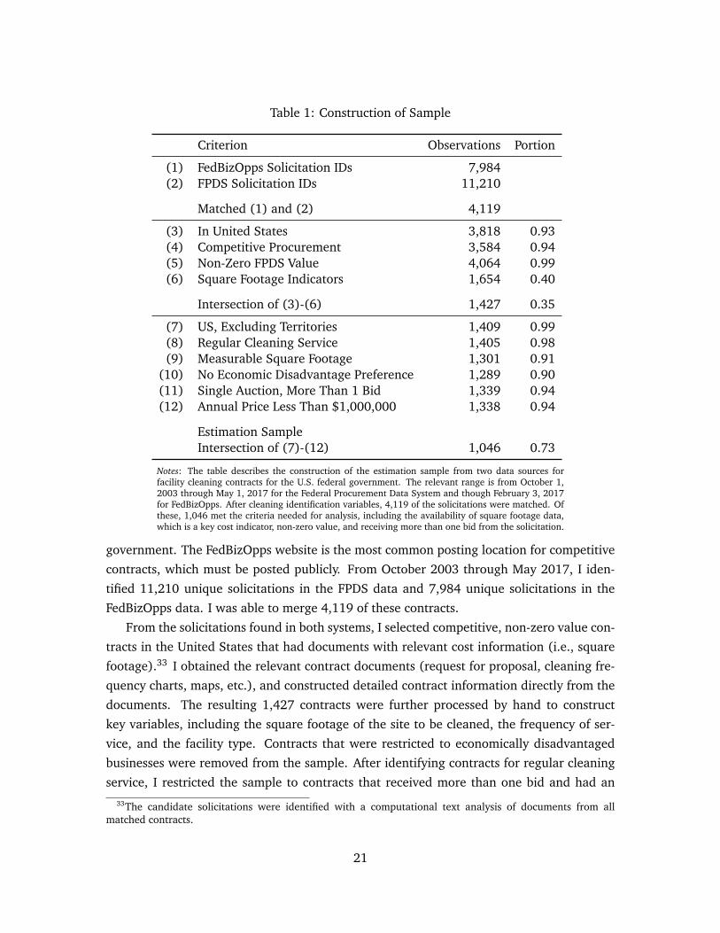
Table 1: Construction of Sample

Criterion Observations Portion

(1) FedBizOpps Solicitation IDs 7,984(2) FPDS Solicitation IDs 11,210

Matched (1) and (2) 4,119

(3) In United States 3,818 0.93(4) Competitive Procurement 3,584 0.94(5) Non-Zero FPDS Value 4,064 0.99(6) Square Footage Indicators 1,654 0.40

Intersection of (3)-(6) 1,427 0.35

(7) US, Excluding Territories 1,409 0.99(8) Regular Cleaning Service 1,405 0.98(9) Measurable Square Footage 1,301 0.91

(10) No Economic Disadvantage Preference 1,289 0.90(11) Single Auction, More Than 1 Bid 1,339 0.94(12) Annual Price Less Than $1,000,000 1,338 0.94

Estimation SampleIntersection of (7)-(12) 1,046 0.73

Notes: The table describes the construction of the estimation sample from two data sources forfacility cleaning contracts for the U.S. federal government. The relevant range is from October 1,2003 through May 1, 2017 for the Federal Procurement Data System and though February 3, 2017for FedBizOpps. After cleaning identification variables, 4,119 of the solicitations were matched. Ofthese, 1,046 met the criteria needed for analysis, including the availability of square footage data,which is a key cost indicator, non-zero value, and receiving more than one bid from the solicitation.

government. The FedBizOpps website is the most common posting location for competitive

contracts, which must be posted publicly. From October 2003 through May 2017, I iden-

tified 11,210 unique solicitations in the FPDS data and 7,984 unique solicitations in the

FedBizOpps data. I was able to merge 4,119 of these contracts.

From the solicitations found in both systems, I selected competitive, non-zero value con-

tracts in the United States that had documents with relevant cost information (i.e., square

footage).33 I obtained the relevant contract documents (request for proposal, cleaning fre-

quency charts, maps, etc.), and constructed detailed contract information directly from the

documents. The resulting 1,427 contracts were further processed by hand to construct

key variables, including the square footage of the site to be cleaned, the frequency of ser-

vice, and the facility type. Contracts that were restricted to economically disadvantaged

businesses were removed from the sample. After identifying contracts for regular cleaning

service, I restricted the sample to contracts that received more than one bid and had an33The candidate solicitations were identified with a computational text analysis of documents from all

matched contracts.

21

annual price of less than $1 million. Table 1 summarizes the construction of the dataset.

I matched the contract-specific dataset with auxiliary datasets of 1) government con-

tracting expenditures at the same location in related products and 2) local labor market

conditions. Local labor market conditions include county-level unemployment from the Lo-

cal Area Unemployment Statistics and the number of NAICS-code level establishments in

the same 3-digit ZIP code from the County Business Patterns data.

4.1.1 Data Cleaning

Though the FPDS data have appealing properties for research broadly, there is a great deal

of measurement error in the data, likely due to user (input) error. As most contracts have

multiple entries and multiple indicators of duration and value within each entry, different

assumptions about data quality could lead to widely different measures of price. As I ob-

tained high-quality measures of price and duration from a second data source, FedBizOpps,

I was able to cross-validate the data and construct preferred measures from the FPDS.

In supplemental work, I detail the steps to cross-check the data and different candidate

measures for price and duration. These comparisons result in the following recommenda-

tions:

• Duration: The maximum observed date in the contract, minus the start date in the firstentry within a contract.

• Price: The price is the value of obligated dollars if it is the same (or within 10 percent) inconsecutive years. If this is not observable, use the maximum value of the three (summed)measures of dollar amounts for the total value of the contract. Divide this by the durationmeasure above to obtain the price.

Any missing values of price or duration in the FedBizOpps data are imputed with the above

values constructed from FPDS. Researchers interested working with the FPDS data may

contact the author for a short paper that details the measurement error in the data and the

accuracy of variables constructed under alternative assumptions.

4.1.2 Institutional Details

Competitive contracts are contracts that are posted publicly and allow open competition

from registered vendors.34 Many of these contracts are posted on the centralized web

portal FedBizOpps.gov, from which I collected the data in this analysis. On the website,

a prospective supplier can view the contract details, including contract duration and the34These contracts fall under three categories: Full and Open Competition, Full and Open Competition after

the Exclusion of Sources, and Competed Under Simplified Acquisition. 86 percent of the contracts deemed Fulland Open Competition after the Exclusion of Sources are listed as a small business set-aside. As 96 percent ofthe contracts are won by small businesses (as determined by the contracting officer), I ignore this distinctionfor the purposes of analysis. See Federal Acquisition Regulation (FAR) Part 5.

22

Table 2: Count of Contracts by Location Type

Category Sub-Category Count

Office (424)Office 221Recruiting Office 203

Field Office (270)Ranger District Office 171Field Office 46Ranger Station 43Work Center 7Reserve Fleet 3

Research (111)Weather Station 43Laboratory 28Research Center 28Plant Materials Center 12

Medical (61)Clinic 36Medical Center 25

Services (59)Service Center 38Vet Center 21

Visitors (41)Recreation Area 18Cemetery 9Visitor Center 7Restroom 4Museum 3

Airport (30)Airport 30

Technical (19)Power Plant 14Surveillance Center 4Data Center 1

Accommodations (18)Housing 14Dormitories 4

Industrial (13)Equipment Center 6Warehouse 6Gym 2

Total 1,046

Notes: The table lists the count of contracts in the estimation sample byfacility type. Types were hand-coded after reading the contract documents.

23

Table 3: Summary Statistics

Mean Min p25 Median p75 Max

Contract Value ($1000s) 190.2 2.91 28.5 50.5 102.0 4882.7Price (Annual, $1000s) 43.9 1.11 7.3 13.2 26.7 976.5Duration (Years) 4.2 0.42 3.0 5.0 5.0 6.5Square Feet (1000s) 25.7 0.14 3.7 7.0 14.5 2031.8Price per Square Foot 2.9 0.16 1.3 2.0 3.1 33.0Number of Bids 6.5 2.00 4.0 5.0 8.0 40.0Weekly Frequency 3.5 0.11 2.0 3.0 5.0 7.0Winner: Num. Employees 61.5 1.00 3.0 14.0 75.0 650.0

Observations 1046

Notes: The table displays summary statistics for key variables in the contract data. Included are outcomes (price,duration, and number of bids), as well as cost characteristics such as the number of square feet and the frequency ofcleaning. The last variable is the size of the winning firm, in terms of number of employees.

square footage of the building, requirements for the job, and a list of interested suppliers.

From the portal, a supplier submits a bid to the contracting office that includes the total

price over the duration of the contract. The contracting office determines the winning

supplier primarily based on the lowest price. By law, the contracting office must justify

selecting other than the lowest-price offer.35

Importantly, contract duration is determined locally by the local contracting officer. As

several industry personnel described to the author, contract duration is a balance between

minimizing the administrative costs of re-contracting and realizing the benefits from re-

competing more frequently. Costs may be increasing with duration because suppliers charge

a premium or because the buyer ends up locked in to a high-cost supplier. This motivates

using this market as a case study for the model developed in this paper. Transaction costs

and competition are key motivating factors for the procuring agencies.

Contracts include specifications for the tasks to be done and their frequencies. For build-

ing cleaning, tasks include mopping, vacuuming carpets, picking up debris, dusting, and

emptying trash cans. For an example list of specifications, see Section H in the Appendix.

The majority of the contracts (694) are for office cleaning, though frequently an office

includes an auxiliary building, such as an exercise room, a bunkhouse, or a small ware-

house. For the empirical analysis of this paper, offices with auxiliary buildings were classi-

fied as Field Offices. Table 2 lists the frequency of each type of site, which are grouped into

ten major categories.36

24

4.1.3 Summary Statistics

Summary statistics for the contracts are displayed in Table 3. Contracts vary in price, dura-

tion, and competition. As shown later in this section, much of the variation in price can be

captured by the square footage of the building and the cleaning frequency.37 The median

contract is relatively inexpensive, as is typical for many commodity-like goods and support

services. For the sample, which removes contracts greater than $1 million per year, the

mean contract is for $44,000 annually. The sample contains 76 contracts with an annual

price greater than $100,000.

One important source of variation in the analysis is in the number of bids received. The

median is 5 bids, and the maximum is 40. Thus, there is a good deal of competition for

these contracts. The variation in the number of bids will help to disentangle the effect of

private costs from unobserved heterogeneity in the structural analysis.

In the last row, the table provides the number of employees for the winning firms. The

winning firms in this dataset are typically small, with a median of 14 employees. Over 25

percent of the winning suppliers have 3 or fewer employees.

Figure 3 displays a scatterplot of the logged values of the winning bids on the y-axis

against the number of bidders on the x-axis. The second panel displays residualized val-

ues for the (log) winning bids. The residuals were constructed from a regression of price

on duration, square footage, cleaning frequency, baseline unemployment, and fixed effects

for facility type. Even after controlling for observable characteristics, there is large varia-

tion in prices for auctions with many bidders. The pattern observed in the scatterplots –

large variation in prices with clustering at the median price, rather than the minimum –

motivates the assumption of unobserved auction-specific heterogeneity used in the model.

Though much of the variation in prices can be explained by observables, there is still resid-

ual variation that is inconsistent with an independent private values model; the model with

multiplicative common shocks fits far better.

The contracts in the dataset have a good deal of variation in duration. Figure 4 pro-

vides a histogram of duration in three-month intervals. There is a good deal of variation

in duration, ranging from 5 months to 6.5 years, though contracts tend to cluster at yearly

increments. Additionally, 53 percent of contracts are for 5 years, which is the typical maxi-

mum contract duration imposed by federal budgeting regulations. Longer durations require

the contracting officer to request and justify an extension. The observed variation in dura-

tion, combined with the presence of a five-year cap on contract duration, help motivate the

counterfactual analysis I perform in Section 6.1, where I consider the value of a flexible-35Based on the guidelines established by FAR and conversations with local contracting offices, the contracting

office will prefer suppliers that have an established history.36For a breakdown of contracts by the issuing department or agency, see Appendix G.1.37Cleaning frequency is encoded as the maximum required weekly frequency in the contract specifications.

25

Figure 3: Price versus Number of Bids

(a) Annual Price

1.0

3.2

10.0

32.0

100.0

316.0

1000.0

10 20 30 40

Number of Bids

Ann

ual P

rice

($10

00, L

og S

cale

)

(b) Residualized Annual Price

−2

−1

0

1

2

10 20 30 40

Number of Bids

Res

idua

lized

Log

Win

ning

Bid

Notes: The figure plots the log annual price against the number of bids received foreach contract. There is a great deal of variation in the annual price, much of whichcannot be explained by observable variables. This is illustrated by the residualized bidsin the lower panel. The R2 of the regression used to construct the residuals, whichincludes duration, square footage, frequency, baseline unemployment, and fixed effectsfor facility type, is 0.74. It is notable that some of the highest and lowest prices arerealized with few bidders.

26

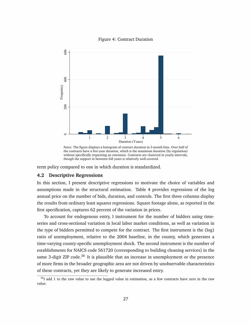
Figure 4: Contract Duration

020

040

060

0Fr

eque

ncy

1 2 3 4 5 6Duration (Years)

Notes: The figure displays a histogram of contract duration in 3-month bins. Over half ofthe contracts have a five-year duration, which is the maximum duration (by regulation)without specifically requesting an extension. Contracts are clustered in yearly intervals,though the support in between full years is relatively well-covered.

term policy compared to one in which duration is standardized.

4.2 Descriptive Regressions

In this section, I present descriptive regressions to motivate the choice of variables and

assumptions made in the structural estimation. Table 4 provides regressions of the log

annual price on the number of bids, duration, and controls. The first three columns display

the results from ordinary least squares regressions. Square footage alone, as reported in the

first specification, captures 62 percent of the variation in prices.

To account for endogenous entry, I instrument for the number of bidders using time-

series and cross-sectional variation in local labor market conditions, as well as variation in

the type of bidders permitted to compete for the contract. The first instrument is the (log)

ratio of unemployment, relative to the 2004 baseline, in the county, which generates a

time-varying county-specific unemployment shock. The second instrument is the number of

establishments for NAICS code 561720 (corresponding to building cleaning services) in the

same 3-digit ZIP code.38 It is plausible that an increase in unemployment or the presence

of more firms in the broader geographic area are not driven by unobservable characteristics

of these contracts, yet they are likely to generate increased entry.38I add 1 to the raw value to use the logged value in estimation, as a few contracts have zero in the raw

value.

27

Table 4: Descriptive Regressions: ln(Annual Price)

OLS-1 OLS-2 OLS-3 IV-1 IV-2

ln(Square Footage) 0.730∗∗∗ 0.658∗∗∗ 0.658∗∗∗ 0.689∗∗∗ 0.687∗∗∗

(0.018) (0.017) (0.017) (0.024) (0.024)

Number of Bids −0.014∗∗∗ −0.009∗ −0.053∗∗ −0.047∗∗

(0.005) (0.005) (0.022) (0.022)

Duration (Years) 0.041∗∗∗ 0.032∗∗ 0.043∗∗∗ 0.033∗∗

(0.015) (0.015) (0.016) (0.015)

ln(Weekly Frequency) 0.459∗∗∗ 0.394∗∗∗ 0.467∗∗∗ 0.407∗∗∗

(0.039) (0.038) (0.041) (0.040)

ln(2004 Unemp.) 0.054∗∗∗ 0.037∗∗∗ 0.080∗∗∗ 0.060∗∗∗

(0.012) (0.012) (0.019) (0.018)

High-Intensity Cleaning 0.586∗∗∗ 0.559∗∗∗

(0.071) (0.075)

Building Type FEs X XObservations 1046 1046 1046 1046 1046R2 0.62 0.71 0.74 0.69 0.73Standard errors in parentheses∗ p < 0.10, ∗∗ p < 0.05, ∗∗∗ p < 0.01

Notes: The table displays estimated coefficients from regressions of log annual price on auction charac-teristics. The variables from specifications OLS-2 and IV-1 are included in the structural model. Theseregressions show that square footage, cleaning frequency, and market characteristics explain much of thevariation in prices. Once square footage, cleaning frequency, and market characteristics are accountedfor, fixed effects for location type add little explanatory power. Specifications IV-1 and IV-2 are two-stageleast squares regressions, where the instruments for the number of bids are monthly (log) county-levelunemployment relative to 2004, the (log) number of NAICS code 561720 establishments in the same3-digit ZIP code in 2004, and an indicator for whether the set-aside was for generic small businesses.

A third instrument is developed from the federal government practice of "setting aside"

certain contracts for firms with particular types of owners. Specialized set asides include

women-owned and veteran-owned small businesses. As we have removed economically

disadvantaged set-asides (e.g., for Economically Disadvantaged Women-Owned Small Busi-

ness) from the sample, it is plausible that the ownership type is uncorrelated with the

underlying cost structure of the participating firms. If the cost structure is independent of

ownership for these firms, then the type of set aside is a valid instrument for price (by af-

fecting entry). This instrument is implemented as a binary variable with the value of 1 if

the set aside is for generic small businesses.

The last three columns report the estimated coefficients from instrument variables re-

gressions. Consistent with endogenous entry, I find a larger negative effect of the number of

bidders on price compared to the corresponding OLS specifications. In the structural model

28

Table 5: Descriptive Regressions: Number of Bids

(1) (2) (3) (4)

Duration (Years) 0.104 −0.017 −0.002 −0.002(0.104) (0.099) (0.099) (0.100)

ln(Square Footage) 0.760∗∗∗ 0.779∗∗∗ 0.834∗∗∗ 0.825∗∗∗

(0.111) (0.106) (0.106) (0.112)

ln(Weekly Frequency) 0.487∗ −0.081 0.009 0.137(0.254) (0.247) (0.253) (0.257)

ln(2004 Unemp.) −0.832∗∗∗ −0.794∗∗∗ −0.793∗∗∗

(0.239) (0.238) (0.238)

ln(Unemployment) 1.415∗∗∗ 1.420∗∗∗ 1.356∗∗∗

(0.232) (0.231) (0.231)

ln(Num. Firms in Zip3) 0.241 0.257∗ 0.276∗

(0.148) (0.148) (0.147)

Generic Set-Aside 1.134∗∗∗ 0.987∗∗∗

(0.350) (0.361)

High-Intensity Cleaning −0.294(0.475)

Building Type FEs XObservations 1046 1046 1046 1046R2 0.06 0.16 0.17 0.19F -statistic 22.2 32.0 25.9 14.7Standard errors in parentheses∗ p < 0.10, ∗∗ p < 0.05, ∗∗∗ p < 0.01

Notes: The table displays estimated coefficients from regressions of the number of bids onauction characteristics and local labor market variables. Specification (3) is equivalentto the first-stage regression of IV-1 in Table 4. Specification (4) includes fixed effects foreach building type.

of Section 5, I explicitly model entry to account for this endogeneity. The main motivating

specification is IV-1, which uses square footage, weekly cleaning frequency, and baseline

(2004) unemployment as controls. To capture variation in the types of buildings and clean-

ing required, IV-1 includes an indicator for "high intensity" cleaning of airports and medical

buildings.39 IV-2 includes indicators for all building types. The inclusion of fixed effects for

all types have low in specifications OLS-3 and IV-2 have a low per-variable impact on R2

and do not have a substantial effect on the estimated coefficients. Therefore, I omit them

from the structural estimation and proceed with the variables used in IV-1.39If separate indicators are estimated for medical buildings and airports, the coefficients on the indicators are

very similar and the coefficients on the other variables are unchanged.

29

Though the linear model does not account for the offsetting effects of duration on price

and (via profits) on entry, the regressions capture a positive relationship between price and

duration. In the structural estimation, I also find a positive and significant direct relation-

ship between duration and price.

In Table 5, I display regressions of the number of bids on auction characteristics and local

measures of unemployment. Specification (3) is equivalent to the first-stage regression in

IV-1 with an F -statistic of 25.9. All three instruments – the unemployment shock, the pres-

ence of existing firms, and a generic set-aside – have the expected positive signs. Though

current unemployment is associated with more bids, higher baseline levels are associated

with fewer bids. I interpret the negative correlation between higher 2004 unemployment

and fewer bids as a reflection of local labor market frictions, leading to reduced competition

and higher wages.

5 Estimation of the Structural Model and Transaction CostsEstimation of the structural model proceeds in three steps. First, I use a parametric max-

imum likelihood to perform joint estimation of entry and bidding. Second, using the

duration decision of the buyer and estimated parameters from the first step, I construct

distribution-free bounds for transaction costs. Third, I construct estimates of transaction

costs by applying a prior over the bounds.

Using the estimated transaction costs and parameters of the model, I address the follow-

ing two questions: (1) How valuable are the non-price terms (duration) of a transaction?

and (2) How important is it to account for transaction costs and duration when estimating

welfare impacts? I address these questions with counterfactual analyses in Section 6.1.

5.1 Estimation of Entry and Bidding

For the contracts in my dataset, I estimate the auction model of Section 3.4. I employ

a parametric approach for parsimony, though the nonparametric identification results pro-

vided earlier, along with robustness checks, suggest that first-order features of the estimated

distributions are not entirely driven by functional form. In this application, there is an added

complication of estimating a duration-dependent distribution of private costs, which would

increase the number of parameters needed for any nonparametric approach.

I employ parameterizations of the objects of interest, where

• Private costs: c ∼Weibull, with mean µ(T ) = µ0 + µ1T and shape α(T ) = α0 + α1T

• Unobserved heterogeneity: U ∼ lnN (−σ2U2 , σ

2U ). (Mean = 1)

• Observed heterogeneity: h(X) = square_footageγ1 · weekly_frequencyγ2

·2004_unemploymentγ3 · γ1[high-intensity_cleaning]4

30

• Entry costs: k(M) = T · square_footageκ1 · weekly_frequencyκ2

·unemployment_shockκ3 · establishmentsκ4 · κ1[generic_set-aside]5

• Entry shock: ε ∼ lnN (µε, σ2ε)

The Weibull distribution is chosen for tractability and flexibility, as it allows the estimated

probability density functions to be either convex or concave. For the distribution of unob-

served heterogeneity, the log-normal distribution was chosen because it best fit the model

out of several choices.40

I allow the parameters of the private cost distribution to vary linearly with duration,

which captures the first-order effects of interest in this model. As I am not taking a stand

on the underlying cost process, I am in this sense estimating a “reduced-form” primitive for

the cost distribution.41

Entry N > n ⇐⇒ E[πn|t] · h(x) · E[U ]− k(m) · ε > 0

Bidder maxb

(b− c) (h(x) · u · t) Pr(bwins|n)

Using the entry and bidding problems above, I estimate these parameters using maxi-

mum likelihood. Entry costs shocks are parameterized as increasing linearly with the du-

ration of the contract.42 Note that square footage and weekly frequency affect the entry

decision by both increasing supply costs (price) and affecting entry costs. One of the com-

putational challenges in maximum likelihood estimation of auction models arises from the

need to invert the bid function, which may be computationally costly. I employ a simple

innovation to greatly speed up this process in the presence of unobserved heterogeneity,

which I provide along with details of the likelihood function in Appendix F.

Table 6 displays the parameter estimates from the first-stage estimation. Square footage,

weekly frequency, and 2004 unemployment are scaled by the mean, so that the estimate of

µ0 is interpreted as the mean annual private cost draw for a zero-duration contract at a

typical location. The mean annual private cost is $18,521 and increases by 2.9 percent per

contract year (µ1/µ0).43 Prices increase with duration due to both the increase in mean

costs and the reduction in variance, as we would expect if cost shocks are not perfectly

correlated over time. Reduced variance is captured by the positive coefficient α1.40Other estimated distributions of unobserved heterogeneity were the gamma distribution and the Weibull

distribution. Both have the desirable properties of support on (0,∞) and can be normalized to have a mean of1.

41For a microfounded model, see Appendix E.42This has the interpretation that entry costs are borne annually, and could reflect the opportunity costs of

other contracts. Allowing a free parameter on the entry costs in estimation generates a coefficient close to one.43For a visual representation of how costs depend on duration, I plot the density of private cost draws for a

one-year and a five-year contract in Figure 8 in the Appendix.

31

Table 6: Parameter Estimates

Group Parameter Variable Estimate 95 Percent C.I.

Private Costs µ0 - 18.521 [16.658, 20.861]µ1 Duration 0.546 [0.085, 0.979]α0 - 4.807 [3.527, 6.969]α1 Duration 0.386 [0.053, 0.674]

Heterogeneity σU - 0.608 [0.572, 0.646]γ1 Square Footage 0.664 [0.627, 0.701]γ2 Weekly Frequency 0.488 [0.411, 0.556]γ3 2004 Unemployment 0.087 [0.070, 0.106]γ4 High-Intensity Cleaning 0.302 [0.187, 0.437]

Entry µε - −0.459 [-0.749, -0.173]σε - 0.649 [0.608, 0.687]κ1 Square Footage 0.543 [0.488, 0.599]κ2 Weekly Frequency 0.542 [0.420, 0.650]κ3 Unemployment Shock −0.309 [-0.449, -0.208]κ4 Establishments −0.066 [-0.108, -0.025]κ5 Generic Set-Aside −0.262 [-0.390, -0.148]

Notes: The table displays maximum likelihood parameter estimates from the structural model. The firstgroup of coefficients indicate how the mean and shape of the private cost distribution change with theduration of the contract. The second set of coefficients indicate the distribution of unobserved auction-specific heterogeneity and how auction-specific common costs vary with observable cost characteristics.The third set of coefficients pertain to entry costs in the model. 95 percent confidence intervals aredisplayed in the last column. As minor data cleaning steps (de-meaning) are data-dependent, confidenceintervals are constructed via 500 bootstrap samples.

As expected, higher values for square footage and weekly frequency increase costs. Con-

sistent with the findings from the descriptive regressions, baseline unemployment and high-

intensity buildings have higher costs. For entry, higher current unemployment and the pres-

ence of more local establishments lower entry costs. Generic small business set-asides also

have lower entry costs, relative to demographic-specific set-asides. Square footage has a

net positive effect on entry, as γ1 > κ1. Supply costs, which are positively correlated with

profits, increase by more than entry costs for square footage. Weekly frequency, on the

other hand, has a net negative effect on entry, as γ2 < κ2. This is consistent with capacity

constraints, as some firms may be limited in the days they are available to clean.

The model fits the data well. In Figure 5, I display actual values for annual prices com-

pared to the predicted values. The R2 for the structural model is 0.71, which compares

favorably to the linear model IV-1 in Table 4. Though the correlation is very strong, unob-

served heterogeneity is important to match the distribution of prices. Unobserved common

costs are economically meaningful, in that they capture approximately 30 percent of the

variance of log prices.

32

Figure 5: Model Fit: Actual Versus Predicted Annual Price

1.0

3.2

10.0

32.0

100.0

316.0

1000.0

1.0 3.2 10.0 32.0 100.0 316.0 1000.0

Predicted Price from Model ($1000s, Log Scale)

Ann

ual P

rice

($10

00s,

Log

Sca

le)

Notes: The figure plots observed prices against predicted prices from the model. TheR2 of the predicted values is 0.71, which compares favorably to the R2 of 0.69 fromthe linear instrumental variables model.

5.2 Estimation of Transaction Costs

In this section, I develop distribution-free bounds for transaction costs based on the esti-

mated parameters for entry and bidding. The buyer’s decision problem is

minT

N∑n=1

E[Bn|n, T, x,m] · E[U |n, T, x,m] · h(x) +δ

T

As demonstrated in Section 3.3.2, the optimality condition can be used to construct

bounds for a contract-specific δ via revealed preference. In my data, contracts are either

set to the nearest monthly or nearest yearly increment, providing a set of tight and loose

bounds, respectively. I assume that that U is not observed prior to entry, i.e. the information

available to potential bidders is captured by X and M , so that E[U |n, t, x,m] = E[U ] = 1.

Finally, to construct expected transaction costs and conduct counterfactuals, I apply a

uniform prior for the density between the distribution-free bounds.44 Using the prior, I

construct point estimates by taking the expectation. In practice, many of the contracts in

my data face a cap on maximum duration of five years, due to federal regulation. For

contracts affected by the cap, only a lower bound for δ can be obtained without additional44The uniform prior is appealing for its transparency and also for the reason that the observed duration is

optimal at the mean transaction cost when buyers can issue contracts in monthly increments. If a left triangularprior were used instead, the optimal monthly-increment contract would be shorter than the observed value forcontracts observed in yearly increments.

33

Table 7: Estimated Transaction Costs ($1000s)

Contract-Specific Measure Median 95 Percent C.I. Mean 25th Pct. 75th Pct.

Transaction Costs 10.3 [3.0, 17.2] 24.1 5.1 21.3Annualized 2.4 [0.7, 4.0] 5.3 1.3 4.7Contract Value 50.5 [46.9, 54.1] 190.2 28.5 102.0Price (Annual) 13.2 [12.3, 13.9] 43.9 7.3 26.7Percent Share of Costs 15.0 [4.9, 21.8] 16.1 9.8 20.5

Aggregate Measure Estimate 95 Percent C.I.

Percent Share of Costs 10.8 [3.8, 20.0]

Notes: Estimated transaction costs are the expectation taken with a uniform prior over the distribution-free bounds identified from the duration decision of the buyer. For T = 5, conservative upper bounds areprojected by assuming that the duration is optimally chosen. The median transaction cost in the data is$10,300. Transaction costs are also expressed as a share of total (buyer) costs. The aggregate share oftotal costs attributable to transaction costs is 10.8 percent, which is calculated by comparing the meanannualized transaction costs to the mean price. Confidence intervals are constructed via the bootstrap.

assumptions. I make the conservative assumption that the chosen duration at five years is

optimal. This generates a relatively conservative upper bound on transaction costs. Many

of the optimal contracts under a higher cap would be likely be longer, implying larger

transaction costs.

Transaction costs are significant in this setting, comprising 10.8 percent of annual costs.

Table 7 contains summary statistics for the estimated transaction costs. To obtain the ag-

gregate share of costs attributable to transaction costs, I divide the mean annualized trans-

action costs by the mean total annual cost (the sum of annualized transaction costs and

the price). Also displayed in the table are the median values for transaction costs, the an-

nualized values, and the corresponding medians for contract value and price. The median

transaction cost is estimated to be $10,300, and the median share of costs attributable to

transaction costs is 15 percent across contracts. 95 percent confidence intervals are cap-

tured via 500 bootstrap samples.

For context, these estimates are not unreasonable given cost estimates provided to the

author by a senior contracting officer. The officer estimated that a simple cleaning contract

would take about three weeks of full-time work for an employee whose salary would be

approximately $75,000 to $90,000. Based on 50 full-time work weeks, this gives a cost

range of $4,500 to $5,400, which is roughly in line with the 25th percentile estimate.

Larger projects may take months of work and multiple officers.

The sequential, revealed-preference approach has the benefit of providing testable impli-

cations of the model via the unconstrained estimates presented here. A finding of negative

transaction costs, which would arise with private costs that fall with duration, would sug-

gest that the tradeoff in this paper is not first-order to contract duration. Instead, the 95

34

percent confidence interval of µ1 has positive support, implying positive transaction costs

only, which is consistent with the model.

In some cases, the estimated transaction costs are quite large as a percent of total costs.

The 95th percentile of share of costs attributable to transaction costs is 32.2 percent. For

these estimates, this is driven by moderate transaction costs realized by low-price projects,

rather than very high absolute costs. For example, contracts with a portion of transaction

costs in the 95th percentile or above (greater than 32.2 percent) have a mean price of

$8,800, which is much smaller than the full-sample mean of $43,900.

5.2.1 Verifying Estimated Transaction Costs

As an exercise to verify the estimated transaction costs, I project the estimates on other

variables not used in the structural estimation. First, I calculate the median transaction costs

by facility type and by department in Table 8. As expected, the highest transaction costs

are among facilities with relatively complicated or technical requirements, such as medical

centers, airports, and technical facilities (e.g., power plants). Simpler settings such as office

cleaning have the lowest estimated transaction costs. In the second panel, I calculate the

median by government department. The Department of Homeland Security has the highest

median transaction costs, at $38,000 per contract. This might be expected given the high

levels of security required at their facilities and the relative lack of institutional knowledge

at the recently-formed department. Conversely, Agriculture and Defense have low median

transaction costs, at $9,300 and $7,200, respectively. After controlling for square footage,

cleaning frequency, and facility type in a regression, Homeland Security has the highest

fixed effect for (log) transaction costs, 91 percent larger than Defense. Agriculture has

lowest fixed effect, 16 percent smaller than Defense.45

In Table 9, I regress the estimated transaction costs on variables excluded from the struc-

tural model. Included variables are the number of pages in the contract, related expendi-

tures and contract modifications46 in the same 9-digit ZIP, and an indicator for whether

the contract falls under the simplified acquisition protocol. One would expect that length-

ier contracts and busier agencies are reflective of higher transaction costs, and that the

simplified acquisition label would reflect lower transaction costs. Indeed, all four enter

with the expected sign. After controlling for square footage and cleaning frequency, high-

expenditure locations are associated with higher transaction costs. Economic theory could

rationalize a sign in either direction, as economies of scale lead to a positive association and

capacity constraints produce a negative one. The negative coefficient on contract modifica-

tions in the fifth specification may reflect economics of scale or simply that lower transaction

costs lead to more contract modifications.45Results available upon request.46Spending and contract actions for other housekeeping services, maintenance, and office furniture.

35

Table 8: Estimated Transaction Costs ($1000s) by Category

(a) Location Type

Type Median Contract Value Size (1000 SF) Count

Medical 38.2 206.0 10.0 61Airport 32.3 254.3 7.8 30Technical 30.6 84.0 15.6 19Industrial 28.4 60.0 27.9 13Accommodations 28.0 121.2 32.0 18Services 18.3 87.7 8.3 59Research 13.2 58.5 6.0 111Visitors 12.8 189.7 6.5 41Field Office 9.1 48.5 8.4 270Office 7.2 35.6 4.8 424

(b) Department

Department Median Contract Value Size (1000 SF) Count

Homeland Security 39.4 269.3 14.6 45GSA 28.8 223.1 12.8 40Veterans Affairs 24.0 143.6 8.8 80Other 20.6 69.2 11.7 24Commerce 13.9 59.7 5.5 78Interior 11.9 70.9 8.9 43Agriculture 9.3 46.7 9.3 347Defense 7.2 35.9 4.2 389

Notes: The table displays the median estimated transaction cost to the buyer. Alsodisplayed are the median contract value, the median square footage of the facility,and the count of observations in the sample. In panel (a), observations are groupedby location type. In panel (b), observations are grouped by contracting department.

36

Table 9: Projecting Transaction Costs on Variables Outside of the Model

(1) (2) (3) (4) (5) (6)

High-Intensity Cleaning 1.446∗∗∗ 1.188∗∗∗ 1.138∗∗∗ 1.020∗∗∗ 1.156∗∗∗ 0.611∗∗∗

(0.144) (0.133) (0.134) (0.138) (0.138) (0.108)

ln(Word Count) 0.085∗∗∗ 0.124∗∗∗ 0.042∗∗

(0.024) (0.023) (0.018)

ln(Related Expenditures) 0.096∗∗∗ 0.073∗∗∗ 0.053∗∗∗

(0.011) (0.023) (0.017)

ln(Related Modifications) 0.283∗∗∗ 0.047 −0.140∗∗

(0.035) (0.071) (0.055)

Simplified Acquisition Ind. −0.693∗∗∗ −0.716∗∗∗ −0.429∗∗∗

(0.090) (0.089) (0.068)

ln(Square Footage) 0.577∗∗∗

(0.026)

ln(Weekly Frequency) 0.510∗∗∗

(0.057)

Observations 1046 1046 1046 1046 1046 1046R2 0.09 0.14 0.13 0.13 0.20 0.54

Standard errors in parentheses∗ p < 0.10, ∗∗ p < 0.05, ∗∗∗ p < 0.01

Notes: The table displays estimated coefficients from regressing estimated log transaction costs on vari-ables outside of the model. These variables are (i) the (log) number of pages in the contract, (ii) loggovernment procurement expenditures at the same 9-digit ZIP for maintenance, office furniture, andother housekeeping services, (iii) the count of contract actions for these expenditures, and (iv) an indi-cator for whether the contract falls under the federal government’s simplified acquisition protocol.

5.3 Robustness

For the structural model, we have proceeded under the assumption that bidders are sym-

metric with respect to private supply costs. In a dynamic setting, the procurement process

might result in asymmetries between bidders that would invalidate this assumption. One

common source of asymmetries in procurement is the presence of an incumbent bidder who

may have an advantage via a relationship-specific investment (e.g., through learning-by-

doing or lowered transaction costs of retaining the same supplier). Additionally, competing

bidders may retain some information about competitors if costs are correlated over time.47

I check for the presence of asymmetries by comparing the expected win percentage

under symmetry (based on the number of bidders) to the win percentage for incumbent

suppliers in follow-on contract. I identify follow-on contracts in the analysis sample by find-

ing contracts that have a single active supplier on another contract in the same 9-digit ZIP

code within the prior year (and starting at least thirty days before). The prior contract may

be any of the approximately 11,000 cleaning contracts in the FPDS data. I also construct a47Saini (2012) discusses the literature on endogenous asymmetries and evaluates a model in which capacity

constraints hurt the winning bidder.

37

Table 10: Test for Asymmetry: Do Incumbents Have an Advantage?

Follow-On Contracts Symmetric Win Rate Incumbent Win Rate N t-Statistic

Estimation Sample 22.4 21.7 175 (0.20)Extended FPDS Sample 27.8 26.3 845 (1.00)

Notes: The table displays the results of a test for asymmetry in performance by incumbent bidders. Theexpected win rate (percent) for symmetric bidders, based on the number of bids, is compared to theobserved win percentage by incumbent bidders. The t-statistics indicate no significant difference in eithersample. The first sample is follow-on contracts in the estimation sample, and the second sample uses thesame criteria for all FPDS building cleaning contracts. Follow-on contracts are identified as contracts thathave a single leading contract for the same agency in the same nine-digit zip code. A leading contract isone that is active in the year prior to the start of the follow-on contract and begins at least thirty daysprior to the start of the follow-on contract.

broader set of follow-on contracts from the extended FPDS sample.

Table 10 compares the expected win percentage for symmetric bidders to the actual win

percentage for incumbent bidders in identified follow on contracts. There is no significant

difference between the two, suggesting that the incumbency advantage is not first-order in

this setting. I obtain similar results for the 175 contract in the estimation sample and the

845 contracts from the broader FPDS sample.48 There are a priori reasons to believe that the

incumbency advantage is not large for competitive federal procurement, as, per regulation,

the agencies are mandated to seriously consider all qualified bidders and, in most cases,

select the lowest price. The degree of relationship-specific investments in facility cleaning

is likely to be low, as the menu of services tend to be standardized.

As a second test, I include a dummy for whether the contract is an identified follow-

on contract in the descriptive regressions to determine if variation in prices and entry are

explained by the presence of an incumbent bidder. None of the coefficients on the dummy

are significant, and its inclusion does not meaningfully change any of the coefficients of

interest. For these regressions, see Appendix G.4. The results of these tests are consistent

with the maintained assumption of no endogenous asymmetries.

A additional general concern might be that there is heterogeneity in supplier types. The

above tests for endogenous asymmetries are also valid tests for exogenous asymmetries

in supplier types. Lower-cost types would be more likely to win the first contract in the

identified set of follow-on contracts, generating a correlation in win rates over time. Thus,

the above findings are consistent with symmetry across suppliers more generally. In contrast

to many other industries, there is no great distinguishing factor that separates types of

building-cleaning firms, and it is reasonable to expect that production is roughly constant

returns-to-scale. This makes the empirical setting a nice fit for the model.48As I only observe winning bidders, I am unable to adjust for when a supplier does not bid on a follow-on

to the supplier’s current contract.

38

Table 11: Effects of Standardized Terms

T Total Cost 95 Percent C.I. Price Trans. Cost Affected Change to δ′

1 36.0 [11.9, 54.4] −11.9 353.9 1018 −60.62 9.7 [3.1, 14.6] −8.0 126.9 992 −32.63 3.1 [1.0, 4.7] −4.2 51.3 907 −15.74 1.4 [0.4, 2.3] −0.4 13.5 992 −9.35 1.6 [0.5, 2.8] 3.2 −9.2 496 −13.36 2.7 [0.9, 4.4] 6.8 −24.4 1041 −27.4

Notes: The table displays the resulting percent changes in total costs, prices, and annualized transac-tion costs when all contracts are issued in standardized durations corresponding to T . For a uniformduration policy of 4 years or less, the average price paid decreases and the amount spent on trans-action costs increases. Affected contracts are the count of those that are displaced from the optimalduration. The final column displays the reduction in transaction costs that would render a uniformpolicy equivalent to the existing policy in terms of buyer costs. Confidence intervals are reported fortotal costs and are constructed via the bootstrap.

6 How Impactful is the Duration Margin?

6.1 The Value to the Buyer: Flexible versus Standardized Terms

When the buyer can adjust the non-price terms of a contract, the buyer can minimize ex-

pected costs for each transaction. This flexibility provides a cost-minimizing advantage to

the firm. In many settings, contracts terms are standardized. For example, a three-year con-

tract is the industry standard for office supplies. The structural model allows us to estimate

how costly such standard-duration contracts would be in the empirical setting of this paper,

conditional on fixed transaction costs.

Though moving away from the optimal duration will raise costs, one might expect that

by simplifying the contracting procedure, transaction costs would fall. Thus, it is worth-

while investigating by how much transaction costs would need to fall to offset the increased

costs arising from a standardized policy. The compensating transaction cost, δ′, makes the

firm (the government, in this case) indifferent between the flexible-duration and standard-

duration policies.

Table 11 reports the impact on aggregate buyer costs by moving to standardized terms

of yearly increments. Total costs would increase substantially, by 36 percent, if all contracts

were issued in one-year terms. This is not surprising, as the median duration in the data is

5 years and standardization would result in much more frequent contracting. On the other

hand, standard durations of 4 years or 5 years would have a small impact, increasing buyer

costs by less than two percent.49

In the final column of Table 11, I report the change in transaction costs that would make49Recall that a conservative assumption was used to calculate transaction costs, so the impacts on total costs

are also conservative.

39

the standardized term policy equivalent to the flexible term policy. For a four-year standard

terms, the necessary reduction in transaction costs is modest. If the government could

reduce transaction costs by 10 percent by implementing a standardized four-year duration

policy for these services, the results suggest that it would be beneficial to do so.

These results suggest that flexible terms may be quite valuable, compared to a poorly-

chosen standard (e.g., one year or two years in this setting). Thus, knowledge of the rele-

vant cost structure and transaction costs is important for setting non-price terms. However,

an intelligently-chosen standard may be cost-effective, as the required reduction in transac-

tion costs to offset the costs of standardization is modest for a four-year standard.

A related question to standardized terms is that of a cap on maximum duration, similar

to the five-year cap imposed by government-wide budgeting regulations in my data. This

is analogous to the imposition of standard terms on only a subset of contracts. In Section

G.3 of the Appendix, I provide a detailed breakdown of the effects by whether duration is

increased or decreased by the standard, which provides insight into the cost of the cap.50

6.2 The Impact to the Econometrician: Welfare Analysis with TransactionCosts

Transaction costs are important to welfare analysis as they can constitute a substantial

portion of total costs and affect how equilibrium prices respond to a change in the economic

environment. When transaction costs are unaffected by a policy change, a welfare analysis

that omits transaction costs will misstate the impact for two reasons. First, the measured

impact on prices should be weighted by the share of total costs attributable to prices. That

is, the impact should be discounted toward zero by the share attributable to (unaffected)

transaction costs. Second, market participants adjust equilibrium behavior in response to

the change. The choice of duration provides an additional margin of adjustment, improving

welfare compared to an analysis that takes duration as fixed.

When transaction costs are affected by a policy change, the above two forces also affect

welfare estimates. Changes to transaction costs should be directly accounted for in the

welfare calculation, and any such changes allow for new duration and price choices that

may improve welfare. Consider two typical forms of welfare analysis: an event study and

a counterfactual simulation with a structural model. For both approaches, assume that

transaction costs and the frequency margin are ignored. Any counterfactual evaluation in

the structural model will find no impact due to transaction costs, as they are outside of the

model. The event study, which makes use of observable responses to a policy change, will

capture the impact of transaction costs on prices and, if measured, duration. However, the

direct impact on transaction costs will be left out.50Table 14 reports averages by contract, rather than in aggregate, which is why the numbers differ slightly

from those in Table 11.

40

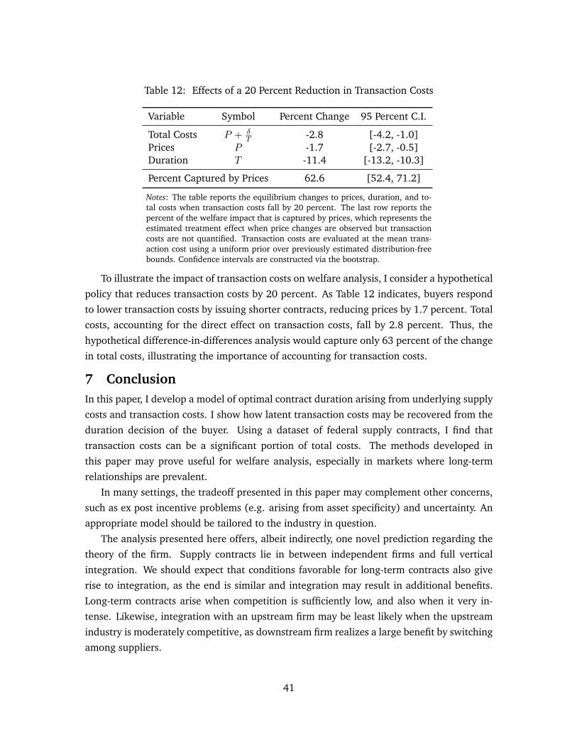
Table 12: Effects of a 20 Percent Reduction in Transaction Costs

Variable Symbol Percent Change 95 Percent C.I.

Total Costs P + δT -2.8 [-4.2, -1.0]

Prices P -1.7 [-2.7, -0.5]Duration T -11.4 [-13.2, -10.3]

Percent Captured by Prices 62.6 [52.4, 71.2]

Notes: The table reports the equilibrium changes to prices, duration, and to-tal costs when transaction costs fall by 20 percent. The last row reports thepercent of the welfare impact that is captured by prices, which represents theestimated treatment effect when price changes are observed but transactioncosts are not quantified. Transaction costs are evaluated at the mean trans-action cost using a uniform prior over previously estimated distribution-freebounds. Confidence intervals are constructed via the bootstrap.

To illustrate the impact of transaction costs on welfare analysis, I consider a hypothetical

policy that reduces transaction costs by 20 percent. As Table 12 indicates, buyers respond

to lower transaction costs by issuing shorter contracts, reducing prices by 1.7 percent. Total

costs, accounting for the direct effect on transaction costs, fall by 2.8 percent. Thus, the

hypothetical difference-in-differences analysis would capture only 63 percent of the change

in total costs, illustrating the importance of accounting for transaction costs.

7 ConclusionIn this paper, I develop a model of optimal contract duration arising from underlying supply

costs and transaction costs. I show how latent transaction costs may be recovered from the

duration decision of the buyer. Using a dataset of federal supply contracts, I find that

transaction costs can be a significant portion of total costs. The methods developed in

this paper may prove useful for welfare analysis, especially in markets where long-term

relationships are prevalent.

In many settings, the tradeoff presented in this paper may complement other concerns,

such as ex post incentive problems (e.g. arising from asset specificity) and uncertainty. An

appropriate model should be tailored to the industry in question.

The analysis presented here offers, albeit indirectly, one novel prediction regarding the

theory of the firm. Supply contracts lie in between independent firms and full vertical

integration. We should expect that conditions favorable for long-term contracts also give

rise to integration, as the end is similar and integration may result in additional benefits.

Long-term contracts arise when competition is sufficiently low, and also when it very in-

tense. Likewise, integration with an upstream firm may be least likely when the upstream

industry is moderately competitive, as downstream firm realizes a large benefit by switching

among suppliers.

41

ReferencesARADILLAS-LÓPEZ, A., A. GANDHI, AND D. QUINT (2013): “Identification and Inference in

Ascending Auctions With Correlated Private Values,” Econometrica, 81, 489–534.

ATALAY, E., A. HORTAÇSU, M. J. LI, AND C. SYVERSON (2017): “How Wide Is the Firm

Border?” National Bureau of Economic Research.

BAKOS, Y. AND E. BRYNJOLFSSON (1999): “Bundling Information Goods: Pricing, Profits,

and Efficiency,” Management Science, 45, 1613–1630.

BEGGS, A. AND P. KLEMPERER (1992): “Multi-Period Competition with Switching Costs,”

Econometrica, 60, 651.

CABRAL, L. (2016): “Dynamic Pricing in Customer Markets with Switching Costs,” Reviewof Economic Dynamics, 20, 43–62.

CANTILLON, E. AND M. PESENDORFER (2006): “Combination Bidding in Multi-Unit Auc-

tions,” Manuscript.

CARLTON, D. W. AND B. KEATING (2015): “Antitrust, Transaction Costs, and Merger Simu-

lation with Nonlinear Pricing,” Journal of Law and Economics, 58, 269–289.

COASE, R. (1960): “The Problem of Social Cost,” Journal of Law and Economics, 3, 1–44.

COASE, R. H. (1937): “The Nature of the Firm,” Economica, 4, 386.

DUBÉ, J.-P., G. J. HITSCH, AND P. E. ROSSI (2009): “Do Switching Costs Make Markets

Less Competitive?” Journal of Marketing Research, 46, 435–445.

DYE, R. A. (1985): “Optimal Length of Labor Contracts,” International Economic Review,

26, 251.

ELZINGA, K. G. AND D. E. MILLS (1998): “Switching Costs in the Wholesale Distribution of

Cigarettes,” Southern Economic Journal, 65, 282.

FARRELL, J. AND P. KLEMPERER (2007): “Coordination and Lock-In: Competition with

Switching Costs and Network Effects,” in Handbook of Industrial Organization, Elsevier,

vol. 3, 1967–2072.

GRAY, J. A. (1978): “On Indexation and Contract Length,” The Journal of Political Economy,

1–18.

GREENSTEIN, S. M. (1993): “Did Installed Base Give an Incumbent Any (Measureable)

Advantages in Federal Computer Procurement?” The RAND Journal of Economics, 24, 19.

GURIEV, S. AND D. KVASOV (2005): “Contracting on Time,” American Economic Review,

1369–1385.

42

HOLMSTROM, B. (1983): “Equilibrium Long-Term Labor Contracts,” The Quarterly Journalof Economics, 98, 23.

HU, Y., D. MCADAMS, AND M. SHUM (2013): “Identification of First-Price Auctions with

Non-Separable Unobserved Heterogeneity,” Journal of Econometrics, 174, 186–193.

JOSKOW, P. L. (1987): “Contract Duration and Relationship-Specific Investments: Empirical

Evidence from Coal Markets,” The American Economic Review.

KLEMPERER, P. (1995): “Competition When Consumers Have Switching Costs: An Overview

with Applications to Industrial Organization, Macroeconomics, and International Trade,”

The Review of Economic Studies, 62, 515–539.

KRASNOKUTSKAYA, E. (2011): “Identification and Estimation of Auction Models with Unob-

served Heterogeneity,” The Review of Economic Studies, 78, 293–327.

LAFONTAINE, F. AND M. SLADE (2007): “Vertical Integration and Firm Boundaries: The

Evidence,” Journal of Economic Literature, 629–685.

MASTEN, S. E. AND K. J. CROCKER (1985): “Efficient Adaptation in Long-Term Contracts:

Take-or-Pay Provisions for Natural Gas,” The American Economic Review, 1083–1093.

MONTEVERDE, K. AND D. J. TEECE (1982): “Supplier Switching Costs and Vertical Integra-

tion in the Automobile Industry,” The Bell Journal of Economics, 13, 206.

PALFREY, T. R. (1983): “Bundling Decisions by a Multiproduct Monopolist with Incomplete

Information,” Econometrica, 51, 463.

QUINT, D. (2015): “Identification in Symmetric English Auctions with Additively Separable

Unobserved Heterogeneity,” Manuscript.

REY, P. AND B. SALANIE (1990): “Long-Term, Short-Term and Renegotiation: On the Value

of Commitment in Contracting,” Econometrica, 58, 597.

RHODES, A. (2014): “Re-Examining the Effects of Switching Costs,” Economic Theory, 57,

161–194.

ROBERTS, J. W. (2013): “Unobserved Heterogeneity and Reserve Prices in Auctions,” TheRAND Journal of Economics, 44, 712–732.

SAINI, V. (2012): “Endogenous Asymmetry in a Dynamic Procurement Auction,” The RANDJournal of Economics, 43, 726–760.

SALINGER, M. A. (1995): “A Graphical Analysis of Bundling,” Journal of Business, 85–98.

STIGLER, G. J. AND J. K. KINDAHL (1970): The Behavior of Industrial Prices, vol. 90, National

Bureau of Economic Research New York.

43

WALKER, G. AND D. WEBER (1984): “A Transaction Cost Approach to Make-or-Buy Deci-

sions,” Administrative Science Quarterly, 373–391.

WILLIAMSON, O. E. (1979): “Transaction-Cost Economics: The Governance of Contractual

Relations,” Journal of Law and Economics, 233–261.

ZHOU, J. (2017): “Competitive Bundling,” Econometrica, 85, 145–172.

44

A Additional Results for the Simple Model

A.1 Mathematical Illustrations of Predictions

Recall the decision rule for the buyer. The buyer will choose a long-term contract if

E[c2:N ]− E[c2:N ] <δ

2.

First, it is straightforward to see that higher marginal costs, by raising the left hand side

of the above equation, increase the cost of long-term contracts and the likelihood that it

outweighs the savings in transaction costs. An increase in transaction costs raises the RHS

and leads to shorter contracts.

To provide a slightly more formal treatment of the predictions, I repeat them below and

provide mathematical illustrations.

Prediction 1 The optimal duration is increasing with autocorrelation in supply costs.

Suppose that d is a cost process with lower autocorrelation than c, but the same per-period

marginal distribution, i.e. E[d2:N ] = E[c2:N ]. Let d denote the average cost across two

periods. Then it follows that, for N > 3,

E[d2:N ] > E[c2:N ]

=⇒ E[d2:N ]− E[d2:N ] > E[c2:N ]− E[c2:N ].

The marginal cost of long-term contracts is decreasing with the autocorrelation of the cost

process. With greater autocorrelation, long-term contracts are preferred.

Prediction 2 The optimal duration is decreasing in the variance of costs across suppliers,

provided there is sufficient competition (N > 3).

For a simple case, consider location-scale transformations of c, such that d = a + bc and

E[d] = E[c]. Under the marginal cost structure d, a longer contract is chosen if

b · (E[c2:N ]− E[c2:N ]) <δ

2.

As b increases, shorter contracts become more desirable.

Prediction 2’ When costs are bounded from below, the optimal duration is U-shaped in the

variance in costs, provided there is sufficient competition (N > 3).

If we impose the reasonable restriction that costs are bounded from below, greater variance

may induce longer contracts by pushing the expected average price and expected per-period

45

Figure 6: Increased Variance in Cost

Baseline

Increased Variance

δ

2= 0.1

0.00

0.05

0.10

5 10 15 20 25 30

Number of Suppliers

Cha

nge

in E

xpec

ted

Cos

t

Notes: The blue line shows the marginal cost to the buyer of a two-period contractrelative to one-period contracts and is equivalent to the blue line in Figure 2.The red line shows the marginal cost of a longer contract when the costs aredraw from the same distributional family (the beta distribution) with 11 percentgreater variance.

price close to the lower bound. Let c denote per-period marginal costs with a lower bound

at 0, and let σ represent its standard deviation. Then, when N > 3,

limσ→∞

E[c2:N ] = limσ→∞

E[c2:N ] = 0.

As E[c2:N ]−E[c2:N ]→ 0, long-term contracts are optimal in the limit. This effect tends

to dominate as N gets large, as more draws brings the minimum price closer to the lower

bound.

A.2 An Increase in the Variance of Costs

Figure 6 displays the change in marginal costs when variance of the cost distribution

increases by 11 percent. The costs are drawn from symmetric beta distributions with

(α, β) = (0.4, 0.4). For N < 12, greater variance increases the cost of long-term contracts.

When N ≥ 13, the winning supplier’s price is close enough to the lower bound to reduce

the cost.

This graph illustrates how the underlying cost structure leads to Prediction 2’, as an in-

crease in variance leads to shorter contracts when competition is lower and longer contracts

when competition is intense.

A.3 The Efficient Case

Though the analysis heretofore has focused on the buyer-optimal case, coinciding with the

typical market outcome, it is worthwhile to consider the efficient case, which minimizes

total social costs. The social planner’s problem is similar to the buyers problem, except that

the social planner will choose a long-term contract if

46

E[c1:N ]− E[c1:N ] <δ

2.

Thus, the social planner’s decision depends on the first-order statistic of cost draws, rather

than the second-order statistic that generates the expected price. For N > 3, these order

statistics have similar qualitative behavior, so the comparative static predictions follow for

the efficient case. However, the efficient contract will not necessarily coincide with the

buyer-optimal contract, raising the question of the allocation of rights to non-price terms of

the transaction.

Figure 7 provides a comparison of the buyer-optimal and the efficient contract. Panel

(a) displays the marginal impact on the price to the buyer of a longer contract with a blue

line. The orange line displays the marginal impact on supply costs. Once N is large enough

(N > 5 in the example), longer contracts have a greater marginal effect on price than

cost. This is intuitive, as the first-order statistic approaches the lower bound faster than the

second-order statistic.

Panel (b) plots the efficient contract with an orange dashed line. It has similar qualita-

tive features to the buyer-optimal contract, displaying the inverse U shape. The efficient

and buyer-optimal contract coincide only when N ∈ {6, 7}. When N = 4, the buyer

would choose a long-term contract when the short-term contract is efficient, and when

N ∈ 8, ..., 21 the buyer would choose a short-term contract when a long-term contract

is efficient. Thus, the buyer-optimal contract may be longer or shorter than the efficient

contract. Information rents from private costs drive a wedge between the buyer-optimal

contract and the efficient contract.

47

Figure 7: Comparing Buyer-Optimal and Efficient Contracts

(a) The Marginal Costs of Longer Contracts

Change in Price

Change in Cost

δ

2= 0.1

0.00

0.05

0.10

5 10 15 20 25 30

Number of Suppliers

Cha

nge

in E

xpec

ted

Cos

t

(b) Efficient versus Optimal Contracts

N=6

N=22

N=4

N=8

1

2

5 10 15 20 25 30

Number of Suppliers

Effi

cien

t Dur

atio

n

Notes: The figure shows the relationship between competition, the marginal costsof longer contracts, and the effect on buyer-optimal and efficient durations. Theblue line in panel (a) shows the marginal cost to the buyer of a two-period con-tract and is equivalent to the blue line in Figure 2. The orange line shows theincrease in marginal social costs of a longer contract. The dash line reflects atransaction cost of 0.20 amortized over two periods. For values of N where theblue line is above the dashed line, N ∈ {6, ..., 21}, the buyer would prefer toissue one-period contracts, as the increase in price is greater than the savings intransaction costs. This range does not coincide with the efficient contract, whichis plotted with the orange dashed line in panel (b). One-period contracts are effi-cient forN ∈ {4, .., 7}. The buyer will select the efficient contract in this exampleonly if N ∈ {6, 7}.

48

B Extensions of the Model: Efficiency and Allocation of RightsIn this section, I explore the relationship between optimal and efficient contract duration

given the more general model of Section 3. It should be noted that the analysis here is

not restricted to the special case of the duration-setting problem, rather, any transaction

characteristic that has a "scale" effect (as duration does on transaction costs) can be related

to this framework. One of the natural extensions is to bundling, where T is the size of a

bundle (determined by the buyer or seller) and δ is the transaction cost for the bundle.

B.1 A Framework Relating Optimal and Efficient Contract Duration

Section 3 presented the buyer-optimal solution to the duration-setting problem. What about

efficiency? The social planner’s concern is expected costs, rather than expected price.51

Let C denote the ex ante expected price conditional on (T,X,M), so that C(T,X,M) =∑Nn=1(E[C(n, T,X,M)]· Pr(N = n|T,X,M)). Thus, the ex ante efficient t contract solves

minTC(T, x,m) +

δ

T

with the first-order condition

dC(T, x,m)

dT|T=t =

δ

t2. (5)

In general, dC(T,x,m)dT |T=t 6=

dP (T,x,m)dT |T=t, which will result in an inefficiency when the

contract is determined by the buyer. As long as interior solutions exist (see Proposition

10), we have the result that the efficient contract t will be longer than the buyer-optimal

contract when dC(T,x,m)dT |T=t <

dP (T,x,m)dT |T=t

Defining the expected seller surplus as E[π(T, x,m)] = P (T, x,m) − C(T, x,m)], we

have the following result:

Proposition 9. When interior solutions to the buyer’s problem and the social planner’s problemexist, the efficient contract will be longer than the equilibrium (buyer-optimal) contract if andonly if the expected seller surplus is increasing at t:

t > t ⇐⇒(dP (T, x,m)

dT|T=t −

dC(T, x,m)

dT|T=t

)> 0

⇐⇒ dE[π(T, x,m)]

dT|T=t > 0

51In this setting, I assume the social planner is limited by information constraints; in this setting the socialplanner cannot observe the private information about sellers’ costs. This reflects the idea that the mechanism(and the associated transaction costs) are important to the truthful revelation of information. A third partywith full information would solve a different problem, awarding the contract to the lowest-cost seller at everyinstant and switching when the net savings outweigh the transaction cost.

49

The existence of interior solutions depends on the concavity of the expected price func-

tion.

Proposition 10. Interior solutions to the buyer’s problem and social planner’s problem exist aslong as the first-order conditions (2) and (5) can be satisfied and P (T, x,m) and C(T, x,m)

are not too concave. In particular, d2P (T,x,m)dT 2 |T=t > −2

t

P (T,x,m)dT |T=t and d2C(T,x,m)

dT 2 |T=t >

−2t

C(T,x,m)dT |T=t. These are the second-order conditions to ensure that first-order conditions

above achieve a minimum.

B.2 Allocation of Term-Setting Rights

Given the general model, we can identify settings in which inefficiency arising from market

power over contract length may be of first-order importance. In this section, I provide

some intuition and a heuristic guide to the assignment of term-setting rights to limit such

inefficiencies.

The buyer’s problem can be written in the following form:

minTP (T, x,m)− C(T, x,m) + C(T, x,m) +

δ

T

= minTE[π(T, x,m)] + C(T, x,m) +

δ

T

Notice that when dE[π(T,x,m)]dT = 0, this problem is equivalent to the social planner prob-

lem. Therefore, when the buyer sets the duration of the contract, these contracts will be

efficient when the seller surplus does not change with the length of the contract. The more

sensitive buyer surplus is to the duration of the contract, the greater the potential for inef-

ficiency.

What about assigning contract term-setting power along with the transaction costs to

the sellers? Sellers solve the problem:

maxT

P (T, x,m)− C(T, x,m)− δ

T

= minT−P (T, x,m) + C(T, x,m) +

δ

T

Sellers solve the social planner problem when dP (T,x,m)dT = 0. Therefore, if price is not

sensitive to contract duration, it is efficient to let the sellers determine the length of the

contract.52

52Sellers have an equivalent rule to Proposition 9: tS > t ⇐⇒ dP (T,x,m)dT

|T=t > 0. This means that either1) tS ≥ t ≥ t, 2) t ≥ t ≥ tS , or 3) tS ≥ t ∩ t ≥ t. The case where both the buyer-optimal and seller-optimalcontract are shorter than the efficient contract is ruled out by the fact that per-period costs must be increasingat the efficient contract for an interior solution.

50

If either price or buyer surplus changes with the duration of the contract, there is po-

tential for inefficiency arising from market power. A simple heuristic to mitigate efficiency

loss is to let sellers determine contract duration when the duration affects price more than

buyer surplus, and to let buyers determine contract duration otherwise.

These heuristics, combined with Proposition 9, provide insight into which settings may

allow for substantive inefficiencies and whether the efficient contract is longer or shorter.

Below, I provide a simple example to illustrate how changing the allocation of rights over

non-price terms, such as duration, may lead to vastly different outcomes.

Example: Markup Pricing Suppose sellers in equilibrium follow a simple markup pricing

rule, P = µC. Then the buyer’s problem is

minTµC(T, x,m) +

δ

T

and the seller’s problem is

minT

(1− µ)C(T, x,m) +δ

T

As µ ≥ 1 in equilibrium, the seller’s problem reverses the sign that expected costs

enter in the objective function. By increasing costs, sellers increase total profits. In

this setting, the buyer should determine the duration. The greater the markup, the

more that the equilibrium contract will diverge from the efficient contract.

B.3 Achieving Efficiency with a Tax

The efficient contract can be achieved with a per-transaction tax (or subsidy) when either

side of the transaction holds the term-setting rights. When the buyer determines the length

of the contract, the efficient per-transaction tax τB solves

τB = t2dE[π(T, x,m)]

dT|T=t

This tax equates the buyer’s problem with the social planner’s problem. Note below how

the tax causes the externality on the seller to drop out at the efficient contract.

t = arg minTE[π(T, x,m)] + C(T, x,m) +

δ + τBT

= arg minTE[π(T, x,m)] +

τBT

+ C(T, x,m) +δ

T

= arg minTC(T, x,m) +

δ

T

51

Analogously, the efficient tax on the seller (when the seller has term-setting rights) is

given by

τS = −t2dP (T, x,m)

dT|T=t

In general, τS 6= τB. A policymaker has a choice between two efficient taxes, with

different effects on tax revenue.

52

C Model Proofs

C.1 Proof of Proposition 1

Rearranging the FOC and taking the total derivative at the optimum (t), we obtain

2tdP (T, x,m)

dT|T=t + t2

d2P (T, x,m)

dT 2|T=t =

dδ

dt

Proof. From the second-order condition for a minimum,

d2P (T, x,m)

dT 2|T=t > −2

δ

t3

.

Therefore

2TdP (T, x,m)

dT|T=t − 2

δ

T<dδ

dt

As the LHS is equal to the first-order condition, it is zero, and therefore dtdδ > 0.

C.2 Proof of Proposition 2

Proof. Taking the total derivative of the first-order condition with respect to M and solving

for dTdM produces

dT

dM=

−d2P (T,X,M)∂T∂M

∂2dP (T,X,M)∂T 2 + 2δ

T 3

. (6)

The denominator is positive, as it is the second-order condition to ensure a minimum.

Therefore, we have the simple relation

sgn

(dT

dM

)= sgn

(−d

2P (T,X,M)

∂T∂M

).

Likewise, this also holds for X.

D Identification Proofs

D.1 Some Lemmas

To demonstrate the following proofs, it will be useful to first introduce several lemmas.

Lemma 1. For symmetric auctions with independent private values, E[b1:N ] = E[c2:N ].

This is a standard result and can be obtained directly by taking the expectation given

the equilibrium bid function. I omit the proof here.

53

Lemma 2. min b1:N = E[c1:(N−1)] for the IPV model when the support of c is bounded frombelow by c > −∞.

Proof. The equilibrium bid function is given by

β(c;N) = c+

∫∞c [1− F (ξ)]N−1dξ

[1− F (c)]N−1

Then the minimum bid is

β(c;N) = c +

∫∞c [1− F (ξ)]N−1dξ

[1− F (c)]N−1

= c +

∫ ∞c

[1− F (ξ)]N−1dξ

= c + ξ[1− F (ξ)]N−1|∞c +

∫ ∞c

ξ(N − 1)f(ξ)[1− F (ξ)]N−2dξ

= c + (0− c) +

∫ ∞c

ξ(N − 1)f(ξ)[1− F (ξ)]N−2dξ

= E[c1:(N−1)]

Where the third line comes from integration by parts. Here we require the assumption that

limξ→∞ f(ξ)[1− F (ξ)]N = 0, so that

ξ[1− F (ξ)]N−1|∞c = limγ→0

[1− F ( 1γ )]N−1

γ− c[1− F (c)]N−1

= limγ→0

−(N − 1)f( 1γ )[1− F ( 1

γ )]N−2

1− c

= 0− c

Lemma 3. The expected k-th order statistic of N draws can be written in terms of the expectedk-th and (k + 1) − th order statistics from N + 1 draws: E[ck:N ] = k

N+1E[c(k+1):(N+1)] +N+1−kN+1 E[ck:(N+1)]

Proof. First, examining the difference between the k-th order statistics of N and N + 1

draws. Expressing E[ck:N ]− E[ck:(N+1)] and rearranging terms gives:

54

E[ck:N ]− E[ck:(N+1)]

=

∫N !

(k − 1)!(N − k)!cf(c)F (c)k−1[1− F (c)]N−kdc−

∫(N + 1)!

(k − 1)!(N + 1− k)!cf(c)F (c)k−1[1− F (c)]N+1−kdc

=

∫ (N !(N + 1− k)

(k − 1)!(N + 1− k)!− (N + 1)!

(k − 1)!(N + 1− k)![1− F (c)]

)cf(c)F (c)k−1[1− F (c)]N−kdc

=

∫(N + 1)!

(k − 1)!(N + 1− k)!cf(c)F (c)k[1− F (c)]N−kdc−

∫kN !

(k − 1)!(N + 1− k)!cf(c)F (c)k−1[1− F (c)]N−kdc

=k

(N + 1− k)

(E[c(k+1):(N+1)]− E[ck:N ]

)Rearranging, we obtain

E[ck:N ] = kN+1E[c(k+1):(N+1)] + N+1−k

N+1 E[ck:(N+1)].

D.2 Proof of Proposition 3

Consider the entry equation

E[πn|n, t] · h(x) · U − k(m) · ε > 0 ⇐⇒ N ≥ n

E[πn|n, t] ·h(x)

k(m)>

ε

U⇐⇒ N ≥ n

For any realization (t, x,m), ∃(t, x′,m′) such that U |(N, t, x,m) = U |(N, t, x′,m′).53 Using

this relation, we can identify h(X) by finding (x′,m′) such that Pr(N ≥ n|t, x,m) = Pr(N ≥n|t, x′,m′) for all N , then calculating

E[B · U · h(x)|N, t, x,m]

E[B · U · h(x′)|N, t, x′,m′]=

E[B|N, t] · E[U |N, t, x,m] · h(x)

E[B|N, t] · E[U |N, t, x′,m′] · h(x′)=h(x)

h(x′)

k(M) is identified by findingh(x)

k(m)=

h(x′)

k(m′)

For a particular realization (n0, t0, x0,m0), normalize h(x0) = 1, and k(m0) = 1, and

E[U |n0, t0, x0,m0] = 1. This pins down the scale of E[B|n0, t0] from the observed transac-

tion price, and the scale of ε is identified from the participation equation. Once h and k are

identified, the distribution of εU is identified directly from the participation equation and

continuous variation in either X or M .

Now that h, k, and the distribution of εU are identified, we consider the identification of

the unobserved components of transaction price.53Here, and once more in the proof, I rely on either h(·) or k(·) having broad support.

55

D.2.1 Identification of Offers and Unobserved Heterogeneity

For any realization (n, t), the expected offer can be identified by finding (x,m) such that

U |(n, t, x,m) = U |(n0, t0,m0, x0). Again, the pair (x,m) is found by setting Pr(N ≥n|t,m, x) = Pr(N ≥ n0|t0,m0, x0). At (x,m), the mean transaction price is equal to the

expected offer scaled by h(X), which is now known:

E[P |n, t,m, x] = E[B|n, t] · E[U |n, t, x,m] · h(X)

= E[B|n, t] · h(X)

As E[B|N,T ] is identified for any (n, t), E[U |N,T,X,M ] is identified from the mean

transaction price at any realization of (N,T,X,M).

To identify surplus, consider the entry condition:

E[πn|n, T ] · h(X)

k(M)>

ε

U

For every (n, x,m) and n′ 6= n, ∃(x′,m′) such that

E[πn|n, T ] · h(x)

k(m)= E[πn′ |n′, T ] · h(x′)

k(m′)

As h(·) and k(·) are identified, E[πn|n,T ]E[πn′ |n′,T ] = R is identified. Likewise, relative profits

E[πn|n,t]E[πn|n,t′] are identified.

D.3 Proof of Proposition 6

The ratio of profits is given by

R =E[πn|n, T ]

E[πn′ |n′, T ]=

1n (E[B|n, T ]− E[C|n, T ])1n′ (E[B|n′, T ]− E[C|n′, T ])

(7)

When the selection mechanism is a symmetric auction. E[B|n, T ] = E[C2:n|T ] and

E[C|n, T ] = E[C1:n|T ]. From here on I suppress notation indicating that costs are condi-

tional on T . From Lemma (3), we haveE[C1:n] = 1n+1E[C2:(n+1)]+

nn+1E[C1:(n+1)]. Plugging

this into the equation for R obtains

R(E[C2:(n+1)]− E[C1:(n+1)]

)= E[C2:n]− 1

n+ 1E[C2:(n+1)]−

n

n+ 1E[C1:(n+1)](

R+n

n+ 1

)E[C1:(n+1)] = E[C2:n]−

(R+

1

n+ 1

)E[C2:(n+1)]

56

Therefore, E[C1:(n+1)] is identified. E[C1:n] is obtained from equation (7).

D.4 Proof of Proposition 7

For each observed sequential value of N ∈ {N, ..., N}, the first-order and second-order

statistics of N draws from the cost distribution are identified. Using the recursive rela-

tionship of order statistics shown in Lemma 3, these are equivalent to identifying the first

N −N + 2 expected order statistics from N draws of C.

D.5 Proof of Proposition 8: Identification with No Instrument

The ratio of second-order statistics is identified by comparing winning bids for different

values of n and n′.

E[Y |n, T,X,M ]

E[Y |n′, T, ,X,M ]=

E[Bn|T,X,M ] · E[U |n, T,X,M ]

E[Bn′ |T,X,M ] · E[U |n′, T,X,M ]=E[C2:n|T,X,M ]

E[C2:n′ |T,X,M ]

Where E[U |n, T,X,M ] = E[U |n′, T,X,M ] = E[U |T,X,M ] by independence and no

selection on unobservables.

From here on, Ci and U may be conditional on (T,X,M). I suppress this in my notation

for clarity. Normalizing E[U ] = 1 pins down the scale of E[C2:n]. 54

Suppose that another (F , G) rationalizes the data. Then

Bn · Ud= Bn · U

Bn′ · Ud= Bn′ · U

Construct bn′ ,˜bn′ , U , and ˜

U as random variables that are independent of and have the

same conditional distributions as their tilde-free counterparts. Then it follows that

(Bn · U) ·(

˜Bn′ ·

˜U)

d=

(Bn · U

)·(Bn′ · U

)=⇒ Bn · ˜

Bn′d= Bn · Bn′

From this relation, we may take the minimum on both sides. By independence and

Lemma 2, I obtain

E[C1:(n−1)] · E[C1:(n′−1)] = E[C1:(n−1)] · E[C1:(n′−1)]

E[C1:(n−1)]

E[C1:(n′−1)]=

E[C1:(n−1)]

E[C1:(n′−1)]

That is, any (F , G) that rationalizes the data has a private cost distribution with the

54Note that, in practice, we may normalize E[U |t, x,m] = 1 for all (t, x,m) realizations. How the mean ofC2:n · U changes is captures in changes to the mean of C.

57

same ratio of first order statistics.

Finally, using the fact that E[C1:(n−1)] = 1nE[C2:n] + n−1

n E[C1:n], we can link together

these ratios when n′ = n+ 1.

1nE[C2:n] + n−1

n E[C1:n]

E[C1:n]=

1nE[C2:n] + n−1

n E[C1:n]

E[C1:n]

=⇒ E[C2:n]

E[C1:n]=

E[C2:n]

E[C1:n]

As we have identified E[C2:n], E[C1:n] and E[C1:(n−1)] is also identified. Seller surplus

is obtained. With sequential values of N ∈ {N, ..., N}, the recursive relationship between

order statistics from Lemma 3 gives the first N − N + 2 expected order statistics from N

draws of C from the identified first-order and second-order statistics.

D.5.1 Identification of Entry Costs

Now that {E[πn(X)]} and E[U |N,T,X,M ] are identified, we can identify entry costs k(M)

from the entry equation.

E[πn|T,X,M ] · E[U |n, T,X,M ] > k(M) · ε ⇐⇒ N ≥ n

Additional assumptions:

1. ε ⊥⊥ (X,M)

2. E[πn|T,X,M ] varies continuously in X conditional on M .

Normalize k(m0) = 1. To identify k(M), find (x,m) and (x′,m0) for any m so that Pr(N =

n|t, x,m) = Pr(N = n, |t, x′,m0). Then

k(m)

k(m0)=

E[πn|t, x,m] · E[U |n, t, x,m]

E[πn|t, x′,m0] · E[U |n, t, x′,m0]

Finally, the distribution of ε is identified once k(M) is identified.

58

E A Model with MicrofoundationsIn the empirical application of this paper, I employ a “reduced-form” approach to a cap-

turing how the distribution of private costs changes with T . Here, I provide a model of

underlying costs that generates both the distribution of costs and how duration affects the

distribution. Suppose that instantaneous costs follow an Ornstein-Uhlenbeck diffusion pro-

cess. The continuous-time cost process Xt is governed by the differential equation

dxt = θ(µ− xt) + σdWt

where Wt is a Wiener process. This process is stationary over t. That is, any contract

with duration T will have the same unconditional distribution as any other contract with

duration T . Define the average cost over time T as

cT =1

T

∫Xtdt

Then cT is Gaussian with mean µ and variance 1T 2

σ2

θ3

(θT + e−θT − 1

). When costs are

Gaussian, E[c1:N (σ)] = E[z1:N ]σ + µ, where z is a standard normal. Define ξ : T → σ. The

efficient contract T solves

minTE[z1:N ]ξ(T ) + µ+

δ

T

This results in the first-order condition

E[z1:N ]ξ′(T ) =δ

T 2

−ξ′(T )T 2 = − δ

E[z1:N ]. (8)

In this case, we obtain a monotonic relationship between the number of bidders and the

optimal duration. Unlike the U-shape models, the microfounded model here does not have

a lower bound on costs.

Proposition 11. The efficient duration is decreasing in the number of bidders.

Proof. ddT

(−ξ′(T )T 2

)= −2T · ξ′(T ) − T 2ξ′′(T ). Combining the second-order conditions

and first-order conditions, we obtain.

E[z1:N ]ξ′′(T ) > − 2

TE[z1:N ]ξ′(T )

=⇒ T 2 · ξ′′(T ) < −2Tξ′(T )

An increase in N increases the RHS of equation 8. As ddT

(−ξ′(T )T 2

)< 0, the optimal

T falls.

59

Further, the analysis above holds for the second-order statistic when N > 3, so we can

extend the results to the buyer-optimal contract:55

Proposition 12. The buyer-optimal duration is decreasing in the number of bidders. It isoptimal for the buyer to issue a permanent contract for N ∈ {2, 3}.

Additionally, in we have that E[z1:N ] < E[z2:N ]. Therefore,

Proposition 13. The efficient duration is less than the buyer-optimal duration.

55For N ∈ {2, 3}, E[z2:N ] > 0.

60

F Likelihood FunctionFor estimation, we obtain the likelihoods for Yn and N given by

fYn|N,X,T,M =

∫fBn|T,N (

y

U

1

h(X))

1

U

1

h(X)fU |N,T,X,M (U)dU

Pr(N = n|T,X,M) =

∫Pr(N = n|U, T,X,M)fU |T,X,M (U)dU

For estimation, I make the assumption that U ⊥⊥ (X,M). As U is not observed by thebuyer when setting T , U ⊥⊥ (T,X,M). This simplifies the problem so that fU |T,X,M (U) =fU (U). The conditional distribution of U used in the likelihood of YN is given by fU |N,T,X,M (u) =Pr(N=n|U,T,X,M)fU (u)

Pr(N=n|T,X,M) . This simplifies so that the joint contribution is given by

fYn|N,X,T,M (yn) · Pr(N = n|T,X,M) =

(∫fBn|T,N (

y

u

1

h(X))

1

u

1

h(X)fU|N,T,X,M (u)du

)Pr(N = n|T,X,M)

=

(∫fBn|T,N (

y

u

1

h(X))

1

u

1

h(X)

Pr(N = n|u, T,X,M)fU (u)

Pr(N = n|T,X,M)du

)Pr(N = n|T,X,M)

=

∫fBn|T,N (

y

u

1

h(X))

1

u

1

h(X)Pr(N = n|u, T,X,M)fU (u)du

With the assumption that the shock ε is independent of (U, T,X,M), we have the fol-

lowing expression for conditional probability of N .

Pr(N = n|U, T,X,M) = Fln ε (lnE[πn|T ] + lnh(X) + lnU − ln k(M))

−Fln ε (lnE[πn+1|T ] + lnh(X) + lnU − ln k(M))

I use the joint likelihood of Yn and N to obtain estimates for cost and entry parameters.

F.1 A Computational Innovation

In this setting, there is a symmetric equilibrium in which each bidder has a monotone bid

function β(·;n) mapping private costs to the submitted bid. The density of an observed bid

is given by

fBn(b) = fc(β−1(b;n))

1

β′(β−1(b;n))

In maximum likelihood estimation of the cost distribution, it is necessary to invert the

bid function to calculate the density. This can be computationally intensive when β does

not have a closed-form solution.

In the presence of unobserved heterogeneity, the density of the observed bid B = B · U

61

is given by the convolution when B ⊥⊥ U .

fB(b) =

∫ u

ufB

(b

u

)1

ufu(u)du

=

∫ u

ufc

(β−1

(b

u;n

))1

β′(β−1

(bu ;n

)) 1

ufu(u)du

Here, the computational burden increases greatly. Integrating out the unobserved het-

erogeneity means that the bid function must be inverted for each value of u within the in-

tegral, in order to calculate β−1(bu ;n

). As the inverse bid function has an analytic solution

for only a few specialized cases, in practice this computation relies on a non-linear equation

solver or an approximation. Thus, the calculations are constrained by the efficiency and

accuracy of such an approach.

One easy-to-implement solution that makes maximum likelihood significantly more tractable

is to use a change-of-variables to calculate the density. Instead of integrating out the un-

observed heterogeneity by integrating over u, replace u with u = bβ(c) and integrate over c.

The density then becomes:

fB(b) =

∫ u

ufC

(β−1

(b

u

))1

β′(β−1

(bu

)) 1

ufu(u)du

=

∫ ψ−1(u)

ψ−1(u)fC(β−1 (β(c))

) 1

β′ (β−1 (β(c)))

β(c)

bfu

(b

β(c)

)(− b

β(c)2β′(c)

)dc

=

∫ c

cfC (c) fu

(b

β(c)

)1

β(c)dc

Note that in this form, there is no need to invert the bid function. As the general form

for the symmetric equilibrium bid function is

β(c) = c+

∫∞c [1− F (z)]n−1

[1− F (c)]n−1,

the primary computational cost is a numerical integration routine. Therefore, the model

is computationally tractable for a vast class of parametric distributions of C and U , as well

as nonparametric approximations such as B-splines.

62

G Supplemental Tables and Figures

G.1 Count of Sites by Government Agency

Table 13: Count of Sites by Contracting Agency

Agency Count Percent

Defense 389 37.2Agriculture 347 33.2Veterans Affairs 80 7.7Commerce 78 7.5Homeland Security 45 4.3Interior 43 4.1GSA 40 3.8Energy 5 0.5Labor 5 0.5Transportation 4 0.4EPA 2 0.2State 2 0.2National Archives 2 0.2CNCS 1 0.1Health And Human Services 1 0.1OPIC 1 0.1Railroad Retirement Board 1 0.1

Total 1,046 100.0

63

G.2 Distributions of Bidder Costs

Figure 8: The Distribution of Bidder Costs

(a) Duration-Dependent Private Costs

0.00

0.03

0.06

0.09

0 10 20 30 40

Private Costs (Annual)

Den

sity

Duration

1

5

(b) Unobservable Auction-Specific Heterogeneity

0.00

0.25

0.50

0.75

0 1 2 3

Multiplicative Unobserved Auction−Specific Costs

Den

sity

Notes: The figure plots the distributions of the unobservable components of bidder costs.Private costs are displayed in panel (a), and the density of unobserved auction-specificheterogeneity is displayed in panel (b). In panel (a), the density is plotted for a one-year contract and a five-year contract. The estimated parameters indicate an increasingmean and a decreasing variance in private costs with contract duration. The densityshifts smoothly between these functions for intermediate values of duration.

64

G.3 Detailed Impacts of Standardized Duration

Table 14: Percent Impact of Uniform Term Policies

T Affected Price Trans. Cost Total Cost Count

1 All −11.2 317.1 33.2 1046

T > T −11.8 334.2 34.9 995T < T 1.5 −36.6 0.6 23

2 All −7.5 108.5 8.8 1046

T > T −8.7 125.4 9.8 930T < T 4.1 −50.5 2.3 62

3 All −3.9 39.0 2.8 1046

T > T −6.3 61.8 3.3 761T < T 5.1 −42.6 2.7 146

4 All −0.4 4.3 1.3 1046

T > T −3.2 24.0 0.7 686T < T 6.0 −39.1 2.9 306

5 All 3.1 −16.6 1.5 1046

T > T −2.0 12.2 0.3 18T < T 6.9 −36.8 3.4 478

Notes: The table displays the average percent changes (by contract,not in aggregate) in total costs, prices, and annualized transactioncosts when all contracts are issued in standardized durations cor-responding to T . For a uniform duration policy of 4 years or less,the average price paid decreases and the amount spent on transac-tion costs increases. The final column lists the count of the affectedcontracts. The first column indicates the group affected by the pol-icy. Rows corresponding to T > T pertain to all contracts that seea reduction in duration, and the reported effects are equivalent toa policy that caps duration at T .

G.4 Incumbency and Asymmetries

In this section, I present regressions for the dependent variables of price and the number

of bids, including an indicator for whether or not a single incumbent bidder was identified

from a previous contract. That is, the indicator equals one if building cleaning services for

the same agency and 9-digit ZIP were performed by a single supplier in the previous year.

The coefficient on this variable is not significant, and its inclusion does not meaningfully

impact the estimated coefficients.

65

Table 15: Descriptive Regressions: Incumbency Check - Price

IV-1 (a) IV-1 (b) IV-1 (c) IV-2 (a) IV-2 (b) IV-2 (c)

Number of Bids −0.053∗∗ −0.052∗∗ −0.052∗∗ −0.047∗∗ −0.046∗∗ −0.046∗∗

(0.022) (0.022) (0.022) (0.022) (0.022) (0.022)

Duration (Years) 0.043∗∗∗ 0.043∗∗∗ 0.043∗∗∗ 0.033∗∗ 0.033∗∗ 0.033∗∗

(0.016) (0.016) (0.016) (0.015) (0.015) (0.015)

ln(Square Footage) 0.689∗∗∗ 0.688∗∗∗ 0.688∗∗∗ 0.687∗∗∗ 0.686∗∗∗ 0.686∗∗∗

(0.024) (0.024) (0.024) (0.024) (0.024) (0.024)

ln(Weekly Frequency) 0.467∗∗∗ 0.467∗∗∗ 0.467∗∗∗ 0.407∗∗∗ 0.407∗∗∗ 0.407∗∗∗

(0.041) (0.041) (0.041) (0.040) (0.040) (0.040)

ln(2004 Unemp.) 0.080∗∗∗ 0.080∗∗∗ 0.080∗∗∗ 0.060∗∗∗ 0.060∗∗∗ 0.060∗∗∗

(0.019) (0.019) (0.019) (0.018) (0.018) (0.018)

High-Intensity Cleaning 0.559∗∗∗ 0.559∗∗∗ 0.559∗∗∗ −0.076 −0.076 −0.077(0.075) (0.075) (0.075) (0.125) (0.125) (0.125)

Follow-On Contract 0.018 −0.003(0.053) (0.050)

Incumbent Winner 0.012 −0.008(0.106) (0.100)

Site Type FEs X X XObservations 1046 1046 1046 1046 1046 1046R2 0.69 0.69 0.69 0.73 0.73 0.73

Standard errors in parentheses∗ p < 0.10, ∗∗ p < 0.05, ∗∗∗ p < 0.01

Notes: The table displays regression results for regressions of log annual price on auction characteristicsand local market characteristics. Specifications IV-1 (a) and IV-2 (a) are two-stage least squares regres-sions and are identical to the descriptive regressions in Table 4. The (b) specifications include an addi-tional regressor indicating whether the contract is a follow-on contract and the (c) specifications includean indicator for whether the contract was won by an incumbent bidder in a follow-on contract.

66

Table 16: Descriptive Regressions: Incumbency Check - Number of Bids

(1) (2) (3) (4) (5) (6)

Duration (Years) −0.002 −0.005 −0.009 −0.002 −0.005 −0.009(0.099) (0.099) (0.099) (0.100) (0.100) (0.100)

ln(Square Footage) 0.834∗∗∗ 0.835∗∗∗ 0.840∗∗∗ 0.825∗∗∗ 0.824∗∗∗ 0.829∗∗∗

(0.106) (0.106) (0.106) (0.112) (0.112) (0.112)

ln(Weekly Frequency) 0.009 0.014 0.010 0.137 0.146 0.141(0.253) (0.253) (0.253) (0.257) (0.258) (0.257)

ln(2004 Unemp.) −0.794∗∗∗ −0.809∗∗∗ −0.813∗∗∗ −0.793∗∗∗ −0.808∗∗∗ −0.811∗∗∗

(0.238) (0.239) (0.239) (0.238) (0.238) (0.238)

ln(Unemployment) 1.420∗∗∗ 1.432∗∗∗ 1.436∗∗∗ 1.356∗∗∗ 1.366∗∗∗ 1.370∗∗∗

(0.231) (0.231) (0.231) (0.231) (0.231) (0.231)

ln(Num. Firms in Zip3) 0.257∗ 0.248∗ 0.250∗ 0.276∗ 0.267∗ 0.269∗

(0.148) (0.148) (0.148) (0.147) (0.147) (0.147)

Generic Set-Aside 1.134∗∗∗ 1.125∗∗∗ 1.131∗∗∗ 0.987∗∗∗ 0.982∗∗∗ 0.985∗∗∗

(0.350) (0.350) (0.350) (0.361) (0.361) (0.361)

High-Intensity Cleaning −0.294 −0.303 −0.305(0.475) (0.475) (0.475)

Follow-On Contract −0.351 −0.353(0.326) (0.326)

Incumbent Winner −0.836 −0.814(0.650) (0.646)

Site Type FEs X X XObservations 1046 1046 1046 1046 1046 1046R2 0.17 0.17 0.17 0.19 0.19 0.19

Standard errors in parentheses∗ p < 0.10, ∗∗ p < 0.05, ∗∗∗ p < 0.01

Notes: The table displays regression results for regressions of number of bids on auction characteristicsand local labor market variables. Specifications (1) and (4) are equivalent to the descriptive regressions(3) and (4) in Table 5. The additional specifications included indicators for whether the contract is afollow-on contract or whether the contract was won by an incumbent bidder in a follow-on contract.

67

H Contract DocumentsThe following page is an example first page from a building cleaning service contract. The

subsequent pages contain an example description of the required services and their respec-

tive frequencies.

68

COMMERCIAL ITEMS SOL NO.: AG-9A63-S-10-0004 PROJ NAME: Janitorial Services UNIT Georgetown Ranger District

8

CONTRACT DOCUMENTS, EXHIBITS OR ATTACHMENTS C.1 SCOPE OF CONTRACT Description of Work: The intent of this contract is to secure services (inclusive of supplies) for normal custodial (janitorial) and routine maintenance service at the Georgetown Ranger District of the Eldorado National Forest. 2 Project Location & Description Location: The project is located on the Georgetown Ranger District, 7600 Wentworth Springs Road, Georgetown, CA 95634. Description: The headquarters office of the Georgetown Ranger District is located at 7600 Wentworth Springs Road, Georgetown, California. Winter working hours are 6:00 a.m. through 5:30 p.m. Monday through Friday from November through May. Summer hours are 7:00 a.m. through 6:00 p.m. Sunday through Saturday. The office building contains approximately 6,376 gross square feet of space. The office is carpeted throughout, expect for restrooms and front reception area. There are 6 restrooms in the building. Any prospective contractor desiring an explanation or interpretation of the solicitation, drawings, specifications, etc., must request it in writing from the Contracting Officer soon enough to allow a reply to reach all prospective contractors before the solicitation closing date. Oral explanations or instructions given before the award of a contract will not be binding. 3 Estimated Start Date & Contract Time Start: January 1, 2010 Time: 9 Months 4 Cleaning Schedule Work Days and Hours. Work shall be performed during Monday through Friday, provided that no work is performed between 7 a.m. and 4:30 p.m. on normal Federal workdays. Regularly scheduled twice weekly work will not be on consecutive days. The contractor may work in the building on weekends and Federal holidays without restrictions to hours. Quarterly cleaning items will be performed the first week (preferably on Friday) of December, March, June, and September. Annual cleaning shall be performed during the first 2 weeks of May.

5 Licenses and Insurance Contractor shall provide proof of Workman’s Compensation. If the contractor is working alone, with no employees, no Workman’s Compensation is required. . 6 Contractor-Furnished Materials and Services 6-1. The Contractor shall provide everything--including, but not limited to, all equipment, supplies (listed below), transportation, labor, and supervision--necessary to complete the project, except for that which the contract clearly states is to be furnished by the Government.

18. TECHNICAL SPECIFICATIONS The janitorial services shall be performed in accordance with the following specifications at the frequencies prescribed.

1. Services Performed Daily - Bid Item #0001

a. Restrooms Clean and sanitize all surfaces including sinks, counters, toilet bowls, toilet

seats, urinals, etc. Clean and sanitize tile walls adjacent to and behind urinals and water closets. Clean and sanitize sanitary napkin receptacles and replace liners. Sweep, mop and sanitize tile floors. Clean and polish mirrors, dispensers and chrome fixtures Empty, clean and sanitize all wastebaskets. Spot clean all other surfaces and dust horizontal surfaces including tops of

partitions and mirrors. Re-stock restroom supplies.

b. Front Foyer and Doors Wash inside and outside of all glass surfaces on entrance doors. Remove dust

and soil from metal frames surrounding entrance glass doors. Vacuum rugs. Sweep and mop tile floors and clean baseboards.

c. Reception Area Vacuum all reception carpeted areas and rugs including edges. Clean and polish all counter surfaces.

d. Drinking Fountains Clean and sanitize drinking fountains.

e. Breakroom Waste Receptacles

Empty all waste receptacles, wash if needed with a sanitizing cleaner.

2. Services Performed Weekly – Bid Item #0002

a. Waste Receptacles Empty all waste receptacles unless needed more frequently. Wash if needed

with a sanitizing cleaner. Change liners only if needed. b. Breakroom

Sweep and mop, use a cleaner that doesn’t require rinsing and is a sanitizer and will not damage the wax. Mop under table, chairs, coffeemaker cabinet, trash can and wheeled carts.

Clean Formica countertops.

Spot clean walls and doors. c. Back Door Foyers

Sweep and mop, use a cleaner that doesn’t require rinsing and is a sanitizer and will not damage the wad. Vacuum rug and clean baseboards.

Spot clean walls and doors. d. Hallways

Vacuum all carpeted areas, including wall edges. Spot clean anytime a stain or soiled area needs cleaning. Tile floors sweep and mop, use a cleaner that doesn’t require rinsing and is a

sanitizer and will not damage the wax. Spot clean walls, doors and partitions that appears to be soiled.

e. Outdoor Waste Receptacles Empty all outdoor waste receptacles and ash trays at the front entrance and

two back entrances. Wash if needed with a sanitizing cleaner. Change liners if needed.

f. Conference Room

Clean and polish conference room tables. Vacuum all carpeted areas, including wall edges and around the edges of all

furniture which is not easily moveable, this includes under desks, tables, chairs etc. All light weight furniture must be moved and vacuumed under. All electrical cords must be picked up and vacuumed under.

Spot clean anytime a stain or soiled area needs cleaning. Vacuum chalk dust out of chalk tray. Wash chalkboard only if it has been

erased by the Forest Service.

g. Copy Machine and Mail room area Vacuum all carpeted areas, including wall edges and around the edges of all

furniture which is not easily moveable, this includes under desks, tables, chairs etc. All light weight furniture must be moved and vacuumed under. All electrical cords must be picked up and vacuumed under.

Spot clean anytime a stain or soiled area needs cleaning. Clean and polish table and counter tops.

3. Services Performed Monthly - Bid Item #0003 a. Dusting

Dust below a 5 foot level. Dust all horizontal and vertical surfaces including but not limited to furniture, baseboards, wood molding, windowsills, bookcases, ledges, signs, wall hangings, photographs, fire alarm boxes, exhibits, top edge of privacy partitions, excluding desktops and computers.

b. Offices

Vacuum all carpeted areas, including wall edges and around the edges of all furniture which is not easily moveable, this includes under desks, tables,

chairs etc. All light weight furniture must be moved and vacuumed under. All electrical cords must be picked up and vacuumed under.

Spot clean anytime a stain or soiled area needs cleaning. Tile floors sweep and mop, use a cleaner that doesn’t require rinsing and is a

sanitizer and will not damage the wax.

c. Outside Foyer and Adjacent Areas Sweep outside area around all outside doors and adjacent area. Pick up any trash laying within 100 feet on the outside of the office building

and parking area. This includes all the bushes and trees.

4. Services Performed Annually - - Bid Item #0004

a. Dusting above 5 feet All horizontal and vertical dust catching surfaces shall be kept free of obvious

dust, dirt, and cobwebs. Dust furniture in all offices above the 5 foot level, including, but not limited to tops of high bookcases and top edge of privacy partitions.

b. Windows

Clean all windows and screens inside and outside of building, with an appropriate glass cleaner. Removing screens on windows that have screens for cleaning.

c. Blinds

Dust, clean and/or vacuum all window blinds. Vinyl blinds may require a liquid cleaner and blinds with fabric may require vacuuming. Clean in accordance with manufacturer’s recommendations by type of fabric or material.

d. Chairs

Vacuum all upholstered chairs. Clean all vinyl covered chairs with an appropriate cleaner for vinyl. Clean chair legs and/or pedestal bases on all the chairs in the office. Wood chairs use an oil, such as lemon oil.

e. Door and Door Frames Clean with appropriate wood/metal cleaner and apply a good penetrating oil to

the wood doors.