Transfer function determinationfor a PM synchronous AC motor

Erik Grassens

DCT 2007.146

Traineeship report

Coaches: Prof. dr. ir. Friso de BoerMr. Greg Heins

Supervisor: Prof. dr. ir. Maarten Steinbuch

Eindhoven University of TechnologyDepartment of Mechanical EngineeringControl Systems Technology Group

Eindhoven, February 2009

Abstract

An axial flux permanent magnet ac brushless drive has limited performance,due to non-smooth torque output. Torque ripple in this system is caused bytwo known sources: current sensor scaling and offset errors, and cogging. Acompensation scheme is in place, but the required parameters need to be deter-mined accurately to minimize the torque ripple. The parameters are estimatedby solving two sub-problems: determining the gain of the total system, anddetermining the gain of the torque sensor. These sub-problems are solved byestimation of the relevant transfer functions, based on frequency response data.Result is that the torque output is substantially smoother, and the operatingrange is increased.

i

Samenvatting

Een axial flux borstelloze motor levert verminderde prestaties, omdat het kop-pel niet constant is. Dit wordt veroorzaakt door fouten in de schaling en offsetvan de stroomsensors, en door cogging. Een compensatieschema is beschik-baar, maar nauwkeurige bepaling van de benodigde parameters is noodzakelijkom het koppel constant te houden. Het schatten van deze parameters wordtopgedeeld in twee deelproblemen: het vinden van de versterkingsfactor van hettotale system, en het vinden van de versterkingsfactor van de koppelsensor. Dezedeelproblemen worden opgelost doormiddel van het schatten van de relevanteoverdrachtsfuncties, gebaseerd op de uit meetdata verkregen frequentierespon-sie. Het resultaat is dat het geleverde koppel aanzienlijk constanter is geworden,waardoor het toepassingsbereik vergroot is.

iii

Contents

Introduction 1

1 Description of the system 3

1.1 Physical setup . . . . . . . . . . . . . . . . . . . . . . . . . . . . . 3

1.2 Theoretical behavior of the system . . . . . . . . . . . . . . . . . 4

1.3 Problem definition . . . . . . . . . . . . . . . . . . . . . . . . . . 5

1.4 Analysis of the torque output . . . . . . . . . . . . . . . . . . . . 6

2 Determination of the total system gain 9

2.1 Current control . . . . . . . . . . . . . . . . . . . . . . . . . . . . 9

2.2 Torque measuring . . . . . . . . . . . . . . . . . . . . . . . . . . . 10

2.3 Inducing harmonics . . . . . . . . . . . . . . . . . . . . . . . . . . 10

2.4 Practical approach . . . . . . . . . . . . . . . . . . . . . . . . . . 10

3 Determination of the torque sensor gain 15

3.1 Dynamics of the system . . . . . . . . . . . . . . . . . . . . . . . 15

3.2 Practical approach . . . . . . . . . . . . . . . . . . . . . . . . . . 16

4 Results 19

4.1 Decoupling of the pulsating torque . . . . . . . . . . . . . . . . . 19

Conclusion 23

Bibliography 25

v

Introduction

Smooth torque is essential in many high-performance motion control applica-tions, such as high quality metal-working, power steering, arc welding, lasercutting and antenna tracking [3, 4]. PM-AC drives are suitable for these appli-cations because they have good characteristics concerning power density, torque-inertia ratio and efficiency [4]. The most important sources of unwanted pulsat-ing torques are cogging, non-ideal back-EMF waveforms, pulse width modulatedcurrent harmonics, and phase commutation events, and especially at low speedsthese cause problems [1]. The torque ripple can be minimized by changing themotor design, which often has a decreased average torque output as result [1, 3],or by pre-compensation in the controller, which requires estimates of the motorparameters to be accurate. The last method might possibly lead to cheapermachines with a higher average torque output [3].

In this work a control based approach is used, which makes it possible to improvethe quality of the torque output without modifying the motor design. Instead,parameter estimation is a crucial step in this method, because pre-compensationrelies on the correctness of the parameters. In the setup used, cogging togetherwith imbalance in the scaling and offset of the current sensors, is responsiblefor most of the pulsating torque in the system. In order to identify which partof the pulsating torque is coming from each source, the torque output mustbe split up in a part depending on the currents, and a part that depends onthe preferred positions of the rotor relative to the stator, and both need to becompensated for.

Chapter 1 will give a description of the setup, as well of its physical configura-tion, as a theoretical formulation. This chapter also gives a problem definition,and the basis for a method to minimize the torque ripple will be founded. Inchapters 2 and 3 the parameters that are needed to use this method, respec-tively the total system gain and the torque sensor gain, will be determined. Atlast, in Chapter 4 these values will be used to minimize the torque ripple andthe final results will be shown.

1

Chapter 1

Description of the system

In order to reduce the torque ripple in the system, it is necessary to have a goodunderstanding of the underlying physics. Therefore, first the configuration ofthe motor will be described, followed by a theoretical analysis of the systems be-havior. The equations that are derived will then be altered so that the problemis well defined. At last the general concept of the solution will be given.

1.1 Physical setup

This section will give a short description of the system that is used in this work,for more details see Heins [2].

The setup is an three phase axial flux permanent magnet ac brushless drive. Inan axial flux drive the rotor is opposite to the stator instead of inside it, as in anconventional electric motor. The rotor has sixteen permanent magnets in eightpole pairs. Therefore, the electrical frequency is eight times higher than themechanical frequency. An offset error in the current sensor or back-EMF willlead to torque ripple at the electrical frequency, which is the eighth harmonic ofthe mechanical frequency. Accordingly, scaling errors will lead to torque rippleat twice the electrical frequency, the sixteenth harmonic.

The output torque is also affected by cogging, which is due to preferred positionsof the rotor relatively to the stator. The permanent magnets on the rotor areattracted to the iron in the coils on the stator. Since the motor has three phasesand sixteen poles, there are 48 stator slots and therefore there are 48 preferredpositions. The torque required to get from the one preferred position to thenext, shows up as ripple in the torque output, and consequently will be a 48th

harmonic.

Although the goal of this work is to produce a smooth, constant torque output,it should be noted that this is not a torque-controlled system. Based on thedesired torque set point and the back-EMF of the motor, the currents that areneeded in each phase are calculated, and form the reference signals that are usedin controlling the motor. The desired currents are then obtained by applyinga feedback loop on these currents, which ideally results in reaching the desired

3

4 Chapter 1. Description of the system

G∗s−1 + + Gs • + gt

1g∗t

I∗i Ii

−~eN~o∗Ts ~eN~o

Ts K ~τc

~τo ~τ∗m

Figure 1.1: Graphical representation of the system and compensation.

torque set point. The currents in all three phases are measured with currentsensors which have some inaccuracy in their scaling and offsets. In order tobe able to operate the motor these are pre-compensated by using data sheetvalues and some manual tuning, which does not lead to an optimal waveformand therefore there is pulsating torque.

In order to be able to operate the motor at more than one angular velocity,an adjustable Eddy current brake is connected to the drive shaft of the motor.Since the torque produced by this brake depends linearly on speed and is fargreater than the torque caused by friction in the system, the assumption is madethat all friction is viscous.

The housing of the motor is fixed to a force table in three points, of which oneis fitted with a piezo sensor which measures the reaction force that results fromthe torque produced by the motor. This sensor is only capable of measuringthe pulsating torque, because it is drifting for low frequencies. This makes itimpossible to quantize the amount of torque that is produced by the motordirectly.

1.2 Theoretical behavior of the system

A graphical representation of the system can be seen in figure 1.1. which showsthe motor inside the dashed line, and the compensation for the current sensorsand torque sensor outside this line. This compensation is based on the datasheets of several components of the motor and its controller and are needed tobe able to operate the motor. However, this compensation is built up out ofseveral components that have not been calibrated together. These parameterswill be denoted with a star, (.)∗, to make a clear distinction between the physicalparameters of the system and their estimates. The part inside the dashed linein figure 1.1, i.e. the hardware of the setup, can be described by

~τo =

(∑row

K •(Ii + ~eN~oTs

)Gs + ~τc

)gt, (1.1)

where

1.3. Problem definition 5

~τo N × 1 vector of the output torque,K N × 3 matrix of the back-EMF,Ii N × 3 matrix of the input currents,

~eN N × 1 vector containing ones,~os 3× 1 vector of the current sensor offsets,Gs 3× 3 diagonal matrix of the current sensor scaling,~τc N × 1 vector of the cogging torque,gt 1× 1 scalar torque sensor scaling.

It should be noted that this equation is in matrix format, since the motor hasthree phases.

1.3 Problem definition

As can be seen in figure 1.1, there is compensated for the current sensor offsetand scaling by respectively subtracting of, and dividing by their estimates. Thetorque sensor scaling is also an estimate, which is compensated for by a similarapproach. By appending (1.1) with this compensation, the following equationis obtained:

~τ∗m =

(∑row

K •(I∗i (G∗

s)−1 + ~eN (~os − ~o∗s)

T)

Gs + ~τc

)gt

g∗t, (1.2)

where

~τ∗m N × 1 vector of the estimated motor torque,I∗i N × 3 matrix of the estimated input currents,~o∗s 3× 1 vector of the estimated current offsets,G∗

s 3× 3 diagonal matrix of the estimated current scaling,g∗t 1× 1 scalar estimate of the torque sensor scaling.

As stated before, the estimates for G∗s, ~o∗s and g∗t are based on data sheet values

and measurements of separate components. Although this is sufficient to getthe motor working, it leaves substantial torque ripple present. In order to geta smooth torque output more accurate values for these parameters need to beobtained.

In order to find these more accurate estimates of the parameters, the system(1.2) is first converted to a different form, which is easier to manipulate. Thisform is presented graphically in figure 1.2. This mathematical equivalent of(1.2) can be written as

~τ∗m =((K • I∗i ) ~αε + K~β + ~τc

)δ, (1.3)

6 Chapter 1. Description of the system

K

I∗i • ~α ε

~β

+ δ~τ∗m

~τc

Figure 1.2: The simplified system and compensation scheme.

where

δ =gt

g∗t, (1.4)

ε = mean(diag

(G∗−1

s Gs

)), (1.5)

~α =diag (G∗−1

s Gs)ε

, (1.6)

~β = Gs (~os − ~o∗s) . (1.7)

In this representation δ and ε are normalized versions of the torque and sensorscaling respectively. Therefore ~α only represents the current imbalance, whichis a necessary property, because in the physical setup the average torque cannot be measured. Writing the system in this form makes it possible to findall required parameters to compensate for the torque ripple caused by currentsensor imbalance and cogging.

1.4 Analysis of the torque output

In order to identify which part of the torque ripple is due to current sensorimbalance and which part to cogging, the pulsating torque must be split up in apart that is linear dependent on the currents and a part that is not. Therefore,the theoretical torque that is produced by the motor, following from (1.3), willbe fitted to the real torque output. The residue will be the part of the torqueripple that is not caused by currents in the motor, e.g. the cogging torque. Itis important to realize that it is not possible to measure the estimated motortorque ~τ∗m directly, because of the drifting torque sensor. Instead the pulsatingtorque ~τ∗p is measured. The relation between the two is given as

~τ∗p = ~τ∗m − ~τ∗r (1.8)

where

~τ∗p N × 1 vector of the estimated pulsating torque,~τ∗r N × 1 vector of the mean torque: δε

∑row

K • I∗i .

Using (1.3) and (1.8) the system can now be written in matrix form as

~τ∗p = X~y + ~τ∗c (1.9)

1.4. Analysis of the torque output 7

where

X =[

K • I∗i K]

(1.10)

~y =[

~α∗

~β∗

]=[

δε (~α− 1)δ~β

](1.11)

In this equation and ~y and ~τ∗c are unknown and need to be solved.

Using a least squares fit, ~α∗ and ~β∗ can be found, which leaves the coggingtorque as a residual. A practical way to do this is by using the Moore-Penrosegeneralized inverse also known as the pseudo-inverse as in [6]. This leads to thefollowing equations:

~y = X+~τ∗p , (1.12)~τ∗c = ~τ∗p −X~y, (1.13)

where (.)+ denotes the pseudo-inverse. Although ~α∗ and ~β∗ can now be found,in order to compensate for the current imbalance ~α and ~β need to be known,which means that δ and the product δε need to be known before the results of(1.12), and therefore also (1.13), are meaningful.

The product δε will be called the total system gain, since it spans the wholesystem, from the currents at the input to the measurement of the torque. Thisscaling factor will be determined in the next chapter by analyzing the transferfunction of the system.

In chapter 3, δ will be determined by using the available information of thedynamics of the system. Since δ determines the quantity of the measured torque,it will be called the torque sensor gain.

Chapter 2

Determination of the totalsystem gain

Although the goal of this work is to produce a smooth constant torque output,the used system is not torque controlled. Instead the currents are controlledwhich leads to a constant average torque. Offset and scaling errors in the currentsensors will cause pulsating effects in the torque output. In order to minimizethese errors the total system gain needs to be determined.

2.1 Current control

As stated before, the currents in the motor are controlled by a feedback controlscheme. This is done following the method described in [2]. For a given torqueset point the current reference signals are calculated, based on the desired torqueand speed normalized back-EMF. By using current sensors feedback is appliedwhich, in the case of an ideal controller, leads to a constant sum of the currentsand therefore a constant torque output.

The back-EMF is determined up to the 144th harmonic by rotating the motorwith an external drive and measuring the the open circuit voltage and angularvelocity, as described in [2], and is verified to be accurate.

The calculated reference signals are then used to control the currents in eachphase of the motor with an PI controller designed using the Zeigler-Nicholsreaction curve method. For a correct implementation of the control scheme itis a requirement that the current sensors are scaled correctly and that thereis no offset present. If this is not the case, the measured current signals willfollow the reference signal but the real currents in the motor will not. Theimplemented controller has a bandwidth of 140 Hz, which limits the maximumangular velocity of the motor to approximately 1 Hz [2].

According to the data sheets, the current sensors convert the currents to avoltage with a factor 0.625

25VA . The voltage divider multiplies this voltage with 2

3in order to make it work with the DSP that was used to implement the control

9

10 Chapter 2. Determination of the total system gain

algorithms. This voltage is than converted to a digital signal by an ADC whichgives 4096

3counts

V . The product gives 22.76 countsA . However, this relies on the

data sheets and might therefore be inaccurate. Measurements showed a valueof 14 counts

A and this value is used for running the motor in experiments.

2.2 Torque measuring

The torque output is measured using a piezo electric force sensor which measuresthe reaction force on the motor housing. The piezo sensor has been calibrated at109 mV

N . When divided by the moment arm of 120 mm this becomes 0.908 VNm .

This can be done because the dynamics of the motor housing are high frequent,so that this part of the setup can be assumed to be static.

2.3 Inducing harmonics

When trying to identify the behavior of the system, an input signal containingharmonics needs to be induced. This is because the system is position based,i.e. for every increment or decrement in the encoder value, a data sample istaken. This implies that when the Fourier transform is applied one does notend up in the frequency domain, but in the harmonics domain. For a constantspeed the frequency response can be obtained by multiplying the harmonics bythis speed. However, due to speed fluctuations resulting from the torque ripple,this is not possible for this setup.

The system identification can be done by inducing the first 144 harmonics inthe current reference signal. Since in this range the current follows the referenceclosely the real currents can be assumed to contain these 144 harmonics. Theharmonics are induced with a random phase in order to avoid peaks in thecurrents due to coinciding maximums of the individual harmonics.

The induced signal can be used to calculate the theoretical electromagnetictorque, which will be compared to the measured torque in the harmonics domain.The magnitude of all harmonics should have the same value, namely that of thetotal system gain δε. However, the harmonics that are multiples of eight mightshow different behavior because of the pulsating torque and cogging that arepresent in the measured torque, but not in the theoretical torque. Thereforethese harmonics should be neglected.

2.4 Practical approach

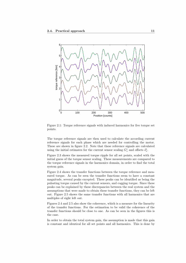
Analysis and control of the axial flux electric drive were done using MATLAB.First the torque reference signals were calculated based on the torque set pointsand the harmonics needed for system identification. Figure 2.1 shows thesereference signals for one electric revolution. There are five torque set pointsranging from 1 Nm to 5 Nm which can be distinguished by the difference intheir magnitudes. These reference signals are calculated for several revolutionsand used at 6 equally spaced speed set points ranging from 0.5 Hz to 1.0 Hz.

2.4. Practical approach 11

0 100 200 300 400 5000

1

2

3

4

5

6

torq

ue r

efer

ence

[Nm

]

Position [counts]

Figure 2.1: Torque reference signals with induced harmonics for five torque setpoints.

The torque reference signals are then used to calculate the according currentreference signals for each phase which are needed for controlling the motor.These are shown in figure 2.2. Note that these reference signals are calculatedusing the initial estimates for the current sensor scaling G∗

s and offsets ~o∗s.

Figure 2.3 shows the measured torque ripple for all set points, scaled with theinitial guess of the torque sensor scaling. These measurements are compared tothe torque reference signals in the harmonics domain, in order to find the totalsystem gain.

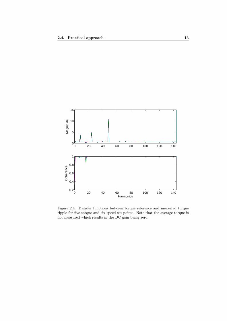
Figure 2.4 shows the transfer functions between the torque reference and mea-sured torque. As can be seen the transfer functions seem to have a constantmagnitude, several peaks excepted. These peaks can be identified as being thepulsating torque caused by the current sensors, and cogging torque. Since thesepeaks can be explained by these discrepancies between the real system and theassumptions that were made to obtain these transfer functions, they can be leftout. Figure 2.5 shows the same transfer functions with all harmonics that aremultiples of eight left out.

Figures 2.4 and 2.5 also show the coherence, which is a measure for the linearityof the transfer functions. For the estimation to be valid the coherence of thetransfer functions should be close to one. As can be seen in the figures this isthe case.

In order to obtain the total system gain, the assumption is made that this gainis constant and identical for all set points and all harmonics. This is done by

12 Chapter 2. Determination of the total system gain

0 100 200 300 400 500−20

−15

−10

−5

0

5

10

15

20

curr

ent r

efer

ence

[A]

Position [counts]

Figure 2.2: Current reference signals with induced harmonics for the threephases and five torque set points.

0 100 200 300 400 500−1.5

−1

−0.5

0

0.5

1

1.5

mea

sure

d to

rque

rip

ple

[Nm

]

Position [counts]

Figure 2.3: Measured torque ripple for five torque and six speed set points.

2.4. Practical approach 13

0 20 40 60 80 100 120 1400

5

10

15

Mag

nitu

de

0 20 40 60 80 100 120 1400.2

0.4

0.6

0.8

1

Coh

eren

ce

Harmonics

Figure 2.4: Transfer functions between torque reference and measured torqueripple for five torque and six speed set points. Note that the average torque isnot measured which results in the DC gain being zero.

14 Chapter 2. Determination of the total system gain

0 20 40 60 80 100 120 1400

0.2

0.4

0.6

0.8

Mag

nitu

de

δε = 0.56285

0 20 40 60 80 100 120 1400.97

0.98

0.99

1

1.01

Coh

eren

ce

Harmonics

Figure 2.5: Transfer functions between torque reference and measured torqueripple with a constant value fitted to them.

a least squares fit. The result is that δε = 0.56 which leaves a residue of about14%. Although this seems quite inaccurate, it is good enough for practicalpurposes.

Chapter 3

Determination of the torquesensor gain

So far the produced torque and position have been considered as outputs ofthe system, but the relation between the two, the dynamical behavior, has notbeen described yet. Because the system is not position controlled the dynamicsmight seem irrelevant at first sight, however, by using their known propertiesthey can be used to find the exact scaling factor of the torque sensor, which isneeded to compensate for the offsets in the current sensor.

3.1 Dynamics of the system

The system can be described by the following differential equation:

~τ∗m = δ

(J

d~θ

dt+ b~θ

), (3.1)

where

~θ N × 1 position vectort timeJ 1× 1 scalar moment of inertiab 1× 1 scalar moment of inertia

Note that although J is a constant, b changes by manipulating the Eddy currentbrake, needed to operate at different set points. By using the Laplace transform(3.1) can be written as:

~τ ∗m = (J∗s + b∗)~θs (3.2)

where

15

16 Chapter 3. Determination of the torque sensor gain

~τ ∗m N × 1 Fourier transform of torque ~τ∗m,~θ N × 1 Fourier transform of position ~θ,s Laplace operator,

and

J∗ = δJ (3.3)b∗ = δb (3.4)

Because multiplication with s is equivalent with taking the derivative to time,(3.2) is in the frequency domain. Therefore the measured torque and positiondata need to be available in the frequency domain too.

Because the data is sampled at constant position intervals instead of constanttime intervals, the data can not be transformed to the frequency domain directlyby applying a FFT algorithm. As a solution is chosen to re-sample the dataat constant time intervals. To make this possible the data can be interpolatedwith a spline, which gives a relatively accurate estimation of the real positionof the system in between two samples.

Using the re-sampled data a frequency response between torque output ~τ ∗m andposition ~θ can be estimated. This frequency response exhibits the behavior of(3.2) and can therefore be used to find J∗, which than can be compared to thevalue obtained in Poels [5]. The quotient than will give δ which follows fromthe definition of J∗.

3.2 Practical approach

When applying this method to the available measurement data, the followingresults were obtained. Figure 3.1 shows the measured frequency responses be-tween torque output ~τ ∗m and ~ω = ~θs for the same set points as used in chapter2. As can be seen the frequency responses are more or less horizontal in thelow frequencies and have a −1 slope between approximately 10 Hz and 100 Hz,which is exactly the behavior that matches (3.2). The coherence shows thatthere is poor linear dependence between between ~τ ∗m and ~ω in the low frequen-cies. This might be explained by the fact that the friction that was assumed tobe viscous, in reality has a substantial part that is non-linear.

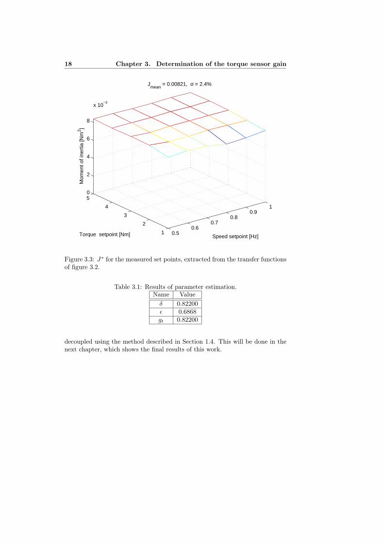
Figure 3.2 shows the transfer functions that result from a least squares fit tothe frequency responses of figure 3.1, made by the frsfit function developed byM. Steinbuch et al. From the parameters of these fitted transfer functions themoments of inertia are extracted for each set point. These are shown in figure3.3.

By calculating the mean of the found moments of inertia for all set points, oneJ∗ can be determined that holds for the system as a whole. The found value is0.00868 Nm2, which is substantially lower than the value of 0.01056 Nm2 foundby Poels [5], that is assumed to be correct.

Following from (3.3), (1.4) and (1.5) all needed parameters can be found. Theseare presented in table 3.1. In order to find Gs and ~os the system needs to be

3.2. Practical approach 17

101

102

−60

−40

−20

0

20

Mag

nitu

de

101

102

0

0.2

0.4

0.6

0.8

1

Frequency [Hz]

Coh

eren

ce

Figure 3.1: Frequency responses between ~τ ∗m and ~ω for five torque and six speedset points.

10−1

100

101

102

−20

−10

0

10

20

30

Mag

nitu

de

10−1

100

101

102

−100

−80

−60

−40

−20

0

Frequency [Hz]

Pha

se [°

]

Figure 3.2: Least squares fit to the frequency responses of figure 3.1.

18 Chapter 3. Determination of the torque sensor gain

0.50.6

0.70.8

0.91

1

2

3

4

50

2

4

6

8

x 10−3

Speed setpoint [Hz]

Jmean

= 0.00821, σ = 2.4%

Torque setpoint [Nm]

Mom

ent o

f ine

rtia

[Nm

2 ]

Figure 3.3: J∗ for the measured set points, extracted from the transfer functionsof figure 3.2.

Table 3.1: Results of parameter estimation.Name Value

δ 0.82200ε 0.6868gt 0.82200

decoupled using the method described in Section 1.4. This will be done in thenext chapter, which shows the final results of this work.

Chapter 4

Results

In the previous two chapters was described how the total system gain and thetorque sensor gain can be determined. This was done in order to follow thetheory presented in Section 1.4. Now that the gains have been found, it is timeto use this theory, to find the exact scaling and offset for each phase, and thecogging torque.

4.1 Decoupling of the pulsating torque

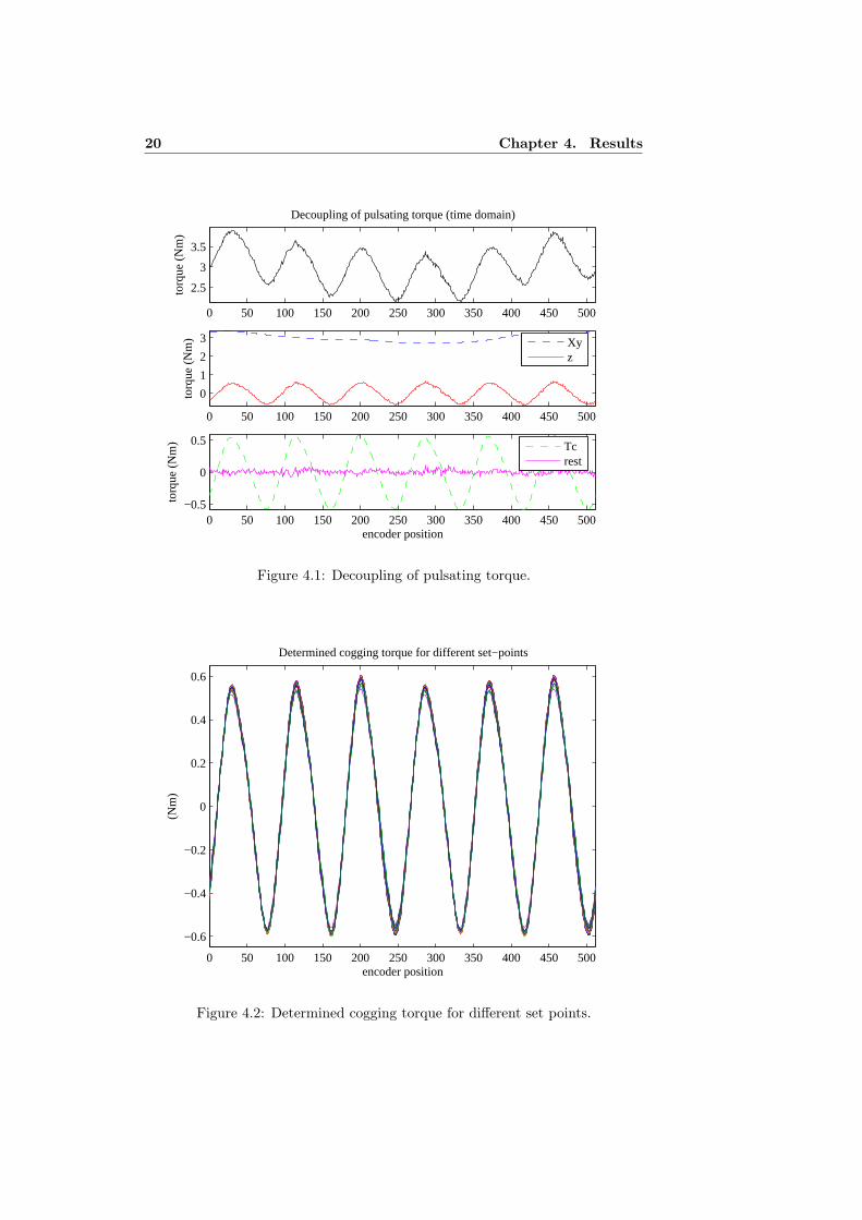
First of all, measurements are taken using the estimated parameters. Compen-sation for the errors in these parameters will take place later. By using (1.12)and (1.13) on a measurement of the pulsating torque, ~y and ~τ∗m can be obtained.Figure 4.1 shows the result for a representative set point. For the real analysisof the system all set points are combined, in order to find values that are suit-able for the whole operating range of the motor. Figure 4.1 shows the measuredtorque, which is split up in the pulsating torque X~y and a residual ~z whichshould be the cogging torque ~τ∗c according to (1.13). In the last part of thisfigure, this residue is split up in the cogging torque, which only consists of the48th harmonic, as was determined during the analysis, and a residue of whichthe source is unknown.

Figure 4.2 shows the cogging torque that is determined this way for every setpoint, in one electrical revolution. At first sight it might look like there are sixperiods, however when looking carefully, one notices that actually two periodsare shown. This indicates that the differences between the three phases on thestator have greater influence on the cogging torque than possible inaccuraciesin the position of the permanent magnets on the rotor. It could also be seenthat there is some deviation between the different torque set points.

Because the cogging torque is supposed to depend only on position and noton speed or electromagnetic torque, it is defined as the mean of the measuredcogging torque for all set points. Figure 4.3 shows the relative error for eachmeasurement compared to this average. Although peaks of up to 8% are presentfor some of the individual set points, the result is considered as sufficient forpractical purposes over the operating range of the motor.

19

20 Chapter 4. Results

0 50 100 150 200 250 300 350 400 450 500

2.5

3

3.5

Decoupling of pulsating torque (time domain)

torq

ue (

Nm

)

0 50 100 150 200 250 300 350 400 450 500

0

1

2

3

torq

ue (

Nm

)

Xyz

0 50 100 150 200 250 300 350 400 450 500−0.5

0

0.5

encoder position

torq

ue (

Nm

)

Tcrest

Figure 4.1: Decoupling of pulsating torque.

0 50 100 150 200 250 300 350 400 450 500

−0.6

−0.4

−0.2

0

0.2

0.4

0.6

Determined cogging torque for different set−points

(Nm

)

encoder position

Figure 4.2: Determined cogging torque for different set points.

4.1. Decoupling of the pulsating torque 21

0 50 100 150 200 250 300 350 400 450 500

−6

−4

−2

0

2

4

6

Cogging torque error for different setpoints

% e

rror

encoder position

Figure 4.3: Cogging torque error for different set points.

Table 4.1: Scaling and offset compensation.Parameter Induced value Calculated value Error

αa 0.8000 0.7717 -3.5%αb 1.1180 1.1035 -1.3%αc 1.1180 1.0884 -2.6%βa 1.0 0.9994 0.1%βb -0.5 -0.5078 1.6%βc -0.5 -0.6205 24.1%

The results in the third column of table 4.1 were obtained from ~y by using(1.11). The second column shows the values that were used to compensate forthe scaling and offset errors in the current sensors during the experiment. Thefourth column shows the relative error of the estimates compared to the newfound values.

By using these new found values and compensation for the cogging torque,the torque ripple can be reduced to one percent of the average torque output.Sensitivity analysis by Poels [5] has shown that it is not possible to reach asituation with less torque ripple by adjusting these parameters, and thereforethis ripple must have another source. Although there is still some torque rippleremaining, the operating range of the motor has increased considerately for thelower speed and torque set points. In these regions it previously would stoprotating because of a lack of torque caused by torque ripple.

Conclusion

The goal of this work was to produce a smooth torque output. The problem hasbeen approached by analyzing the torque ripple and compensating for each of itssources in a appropriate manner. The torque has been split up in a part linearlydepending on the motor currents and a residue containing cogging effects. Thisallowed compensation of each component of the torque ripple right at its source.To make this method work, the total system gain and torque sensor gain neededto be determined.

The total system gain has been determined by analyzing the system’s frequencyresponse. This frequency response, that shows the relation between the the-oretical torque output of the motor and its measured counterpart, has beenobtained by inducing harmonics. By applying a least squares fit on this fre-quency response, a scalar value was determined that describes the total systemgain sufficiently accurate for use in the compensation scheme.

The torque sensor gain has been determined by analyzing the dynamics of thesystem, i.e. the relation between the torque output and position of the system.A transfer function of the dynamics has been fit to the frequency response inorder to find an estimate of the moment of inertia. By comparing this estimateto a more accurate value following from other experiments, the torque sensorgain has been determined. This same fit also shows that the assumption ofviscous friction might be invalid.

These values were used to correct the scaling and offsets of the current sensorsand for cogging torque compensation, which minimized the torque ripple in thesystem. This extended the operating range of the setup for low speeds andtorque set points.

Although the torque ripple is now substantially less than it was before, it has notcompletely gone, which leaves some room for improvement. Since the remainingtorque ripple can not be related directly to a source, there might be compensatedfor it by applying feed forward based on an error signal, such as iterative learningcontrol.

23

Bibliography

[1] M. Aydin, Z.Q. Zhu, T.A. Lipo, and D. Howe. Minimization of coggingtorque in axial-flux permanent-magnet machines: Design concepts. IEEETransactions on Magnetics, 43(9):3614–3622, 2007.

[2] G. Heins. Control methods for smooth operation of permanent magnet syn-chronous ac motors. PhD thesis, Charles Darwin University, 2007.

[3] G. Heins, F.G. de Boer, J. Wouters, and R. Bruns. Experimental validationof reference current waveform techniques for pulsating torque minimizationin pmac motors. 2006.

[4] T.M. Jahns and W.L. Soong. Pulsating torque minimization techniquesfor permanent magnet ac motor drives: A review. IEEE Transactions onIndustrial Electronics, 43(2):321–329, 1996.

[5] P.W. Poels. Cogging torque measurement, moment of inertia determina-tion and sensitivity analysis of an axial flux permanent magnet ac motor.Technical Report DCT 2007.147, Technische Universiteit Eindhoven, 2007.

[6] Sigurd Skogestad and Ian Postlethwaite. Multivariable feedback control:Analysis and design. Wiley, Chichester, second edition, 2005.

25