Solar PhysicsDOI: 10.1007/•••••-•••-•••-••••-•

Transfer of Energy, Potential and Current by Alfven

Waves in Solar Flares

D.B. Melrose1 · M.S. Wheatland1

c© Springer ••••

Abstract Alfven waves play three related roles in the impulsive phase of a solarflare: they transport energy from a generator region to an acceleration region;they map the cross-field potential (associated with the driven energy release)from the generator region onto the acceleration region; and within the acceler-ation region they damp by setting up a parallel electric field that accelerateselectrons and transfers the wave energy to them. The Alfven waves may also beregarded as setting up new closed current loops, with field-aligned currents thatclose across field lines at boundaries. A model is developed for large-amplitudeAlfven waves that shows how Alfven waves play these roles in solar flares. Apicket-fence structure for the current flow is incorporated into the model toaccount for the “number problem” and the energy of the accelerated electrons.

Keywords: solar flares; Alfven waves; electron acceleration

1. Introduction

There are long-standing, unsolved problems in the physics of solar flares. A largefraction of the magnetic energy released in a flare appears in ε = 10 − 20 keVelectrons that produce hard X-rays and type III solar radio bursts. One problemis that there is no satisfactory model for the acceleration of these electrons,which, in the older literature, was referred to as “first phase” acceleration (Wild,Smerd, and Weiss, 1963) and as “bulk energization” of electrons. Runaway accel-eration (Holman, 1985) due to a parallel electric field [E‖] seems the only viableacceleration mechanism, but there is no accepted model for how E‖ 6= 0 is set upand maintained in an acceleration region. There is also a long-standing “num-ber problem” (Hoyng, Brown, and Van Beek, 1976; MacKinnon, and Brown,1989; Bian, Kontar, and Brown, 2010) that can be expressed in various ways; forexample, the rate, N > 1036 s−1, of precipitation of accelerated electrons inferredfrom hard X-ray observations implies a total of 1039 accelerated electrons in aflare of duration 103 seconds, and this exceeds the number of electrons stored inthe entire flaring flux loop, estimated to be 1037 (Emslie, and Henoux, 1995).

1 Sydney Institute for Astronomy, School of Physics,University of Sydney, NSW 2006, Australia email:melrose@physics.usyd.edu.au,m.wheatland@physics.usyd.edu.au

SOLA: Melrose_Wheatland_final.tex; 6 April 2013; 8:45; p. 1

D.B. Melrose, M.S. Wheatland

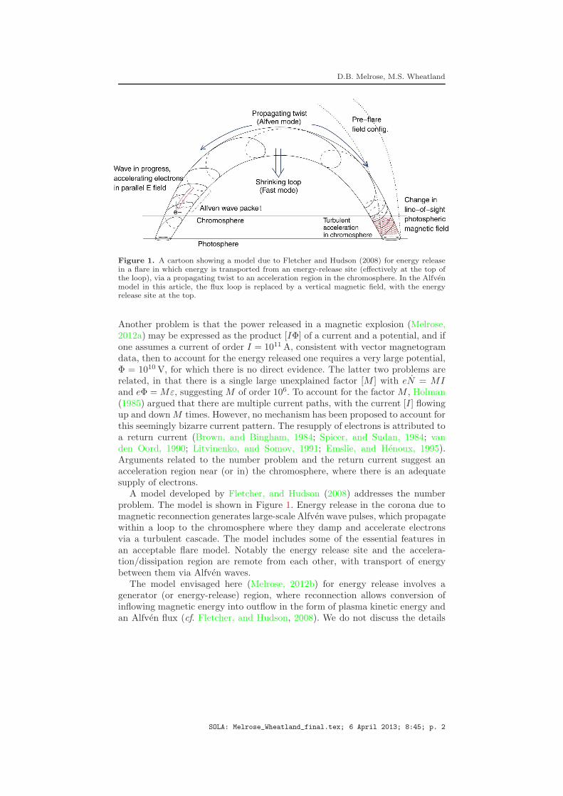
Figure 1. A cartoon showing a model due to Fletcher and Hudson (2008) for energy releasein a flare in which energy is transported from an energy-release site (effectively at the top ofthe loop), via a propagating twist to an acceleration region in the chromosphere. In the Alfvenmodel in this article, the flux loop is replaced by a vertical magnetic field, with the energyrelease site at the top.

Another problem is that the power released in a magnetic explosion (Melrose,2012a) may be expressed as the product [IΦ] of a current and a potential, and ifone assumes a current of order I = 1011 A, consistent with vector magnetogramdata, then to account for the energy released one requires a very large potential,Φ = 1010 V, for which there is no direct evidence. The latter two problems arerelated, in that there is a single large unexplained factor [M ] with eN = MIand eΦ = Mε, suggesting M of order 106. To account for the factor M , Holman(1985) argued that there are multiple current paths, with the current [I] flowingup and downM times. However, no mechanism has been proposed to account forthis seemingly bizarre current pattern. The resupply of electrons is attributed toa return current (Brown, and Bingham, 1984; Spicer, and Sudan, 1984; vanden Oord, 1990; Litvinenko, and Somov, 1991; Emslie, and Henoux, 1995).Arguments related to the number problem and the return current suggest anacceleration region near (or in) the chromosphere, where there is an adequatesupply of electrons.

A model developed by Fletcher, and Hudson (2008) addresses the numberproblem. The model is shown in Figure 1. Energy release in the corona due tomagnetic reconnection generates large-scale Alfven wave pulses, which propagatewithin a loop to the chromosphere where they damp and accelerate electronsvia a turbulent cascade. The model includes some of the essential features inan acceptable flare model. Notably the energy release site and the accelera-tion/dissipation region are remote from each other, with transport of energybetween them via Alfven waves.

The model envisaged here (Melrose, 2012b) for energy release involves agenerator (or energy-release) region, where reconnection allows conversion ofinflowing magnetic energy into outflow in the form of plasma kinetic energy andan Alfven flux (cf. Fletcher, and Hudson, 2008). We do not discuss the details

SOLA: Melrose_Wheatland_final.tex; 6 April 2013; 8:45; p. 2

Alfven Waves in Solar Flares

cross field currents

(energy dissipation)acceleration region

field aligned currents

field aligned currents

cross field currents

coronal generator(energy release)

photosphere(line−tied boundary)

Figure 2. A schematic diagram of the model adopted in this article, as explained in the text.

of the generator region here, but several comments are appropriate. The energyrelease needs to be driven, and one possible mechanical driver is a pressuregradient, associated with collection of dense plasma near the top of the flaringloop (Haerendel, 2001, 2009; 2012, Fletcher, and Hudson, 2008). In this caseone needs to consider the energy and momentum associated with this denseplasma, and how it is transferred to Alfven waves. Our view (Melrose, 2012a,2012b) is that the driver is the Maxwell stress, and that this becomes available asreconnection allows the magnetic figuration to change to a less stressed state. Theenergy and momentum in the plasma then play only a minor role. We identifythe power [IΦ] released to redirection of pre-existing current across field lines inthe generator region, with the electromotive force [Φ] attributed to the rate ofchange of the stored magnetic flux. This cross-field current [I] is assumed to beredirected so that it flows along field lines through an acceleration region, andcloses across field lines in the photosphere, and then flows back to the generatorregion.

A schematic diagram of the new model is shown in Figure 2. The magneticfield is assumed to be vertical, with the top of the figure in the corona, and thebottom at the photosphere. The redirection of current at the coronal generatoris analogous to the redirection of current that occurs in the so-called currentwedge in a magnetospheric substorm (McPherran, Russel, and Aubry, 1973;Paschmann, Haaland, and Treumann, 2002). The physics underlying this effectis related to a conducting boundary (Simon, 1955), which is the plasma wallin a laboratory context, the ionosphere in the magnetospheric context, and thephotosphere in the context of a flare. Specifically, when a current is driven acrossfield lines in the body of the plasma, it closes by flowing along the field linesto a region where the conductivity allows it to close across field lines. FollowingHolman (1985), it is assumed that this redirection occurs M times in a flare,so that the potential imposed at the generator region is Φ/M for each suchredirected current path.

SOLA: Melrose_Wheatland_final.tex; 6 April 2013; 8:45; p. 3

D.B. Melrose, M.S. Wheatland

In this article an analytic model for the large-scale Alfven waves is developedand used to describe various roles that Alfven waves play in such a model. Thefeatures that are new, in the solar context, are the transport of potential alongfield lines, and the setting up of new closed current loops. The electric field inthe wave is expressed in terms of a wave potential, which also determines thefield-aligned current (FAC) density in the wave. The waves map the potential,imposed at the generator region, onto the acceleration region, where the wavesare assumed to damp, converting the cross-field potential at the top of theacceleration region into a field-aligned potential within the acceleration region.Figure 3 illustrates the mapping of the potential and the role of the accelerationregion. With the magnetic field in the vertical direction, the equipotentials shownby dashed lines are vertical above the acceleration region. The potential set upin the generator region (above the top of the diagram) maps along field linesto the acceleration region, where a field-aligned potential is established. Thefield-aligned electric field [E‖] in the region extracts energy from the waves andtransfers it to electrons.

Assuming that current is conserved in an Alfven wave (∇ · J = 0), an Alfvenwave can transfer a FAC from one field line to another, and can transfer across-field current from one location to another, but it cannot introduce anyintrinsically new current. This implies that an Alfven wave that is localized to aflux tube can have no net FAC: the FAC in the wave must change sign across thewavefront, and include equal up and down currents. The up and down FACs inthe wave close across field lines in the generator region and in the photosphere,forming a closed current loop, and transferring the cross field current from oneregion to the other.

The general model for Alfven waves is developed in Section 2, and somerelevant boundary conditions are discussed in Section 3. The model is applied tocylindrical and planar geometries in Section 4. Some aspects of the extensionof the model into the acceleration region are discussed in Section 5, and ageneral discussion of the results is presented in Section 6. The conclusions aresummarized in Section 7.

2. Alfven Waves

The model for Alfven wave adopted here is based on one developed in connectionwith magnetospheric substorms (Vogt and Haerendel, 1998; Paschmann, Haa-land, and Treumann, 2002). Conventional treatments of Alfven waves are basedon MHD or the low-frequency limit of cold-plasma theory, and assume that thewaves are of small amplitude. The approach adopted here applies to Alfven waveseven when neither of these theories is valid, and there is no restriction on thewave amplitude. Our approach is based on two well-known results from orbittheory: the electric and polarization drifts (Northrop, 1963). It allows one toinclude the plasma response to an electric field (and its time derivative) withoutassuming that its amplitude is small.

SOLA: Melrose_Wheatland_final.tex; 6 April 2013; 8:45; p. 4

Alfven Waves in Solar Flares

2.1. Electric and Polarization Drifts

Any electric field, including both the inductive electric field due to the changingmagnetic field, and the electric field in an Alfven wave, can be separated intocomponents perpendicular [E⊥] and parallel [E‖z] to the background magneticfield [B = Bz] which is assumed uniform along the z axis. Subject to relativelyweak conditions (on the slowly time-varying electric field), one has

E = E⊥ + E‖z, E⊥ = −u×B, (1)

with u = E⊥ × B/B2 the electric drift velocity. In MHD, u is interpretedas the fluid velocity, and Equation (1) is attributed to Ohm’s law for infiniteconductivity, which also implies E‖ = 0. The interpretation of u as the electricdrift velocity is different from the usual MHD interpretation: here E implies u

and E‖ is arbitrary, whereas in MHD u implies E with E‖ = 0. The divergenceof the electric field, in the form Equation (1), gives the charge density,

ρ

ε0= −Bz · ω+

∂E‖

∂z, ω = ∇× u, (2)

where ω is the vorticity in a fluid interpretation.A temporally changing (perpendicular) electric field corresponds to a dis-

placement current ε0∂E⊥/∂t, and this causes a polarization drift, which isalong ∂E⊥/∂t at a velocity proportional to the mass to charge ratio. Aftersumming over the contributions of all species of charged particles, this implies apolarization current density

Jpol⊥ =c2

v2AJdispl, Jdispl = ε0

∂E⊥

∂t. (3)

The sum of the two currents in Equation (3) is c2/v20 times Jdispl, where v0 =vA/(1 + v2A/c

2)1/2 is the MHD speed and vA is the conventional Alfven speed.Equation (3) may also be derived using cold-plasma theory, as shown in

Appendix A.

2.2. Wave Equation

Including the polarization current in Ampere’s equation, and combining it withFaraday’s equation, leads to a wave equation for the electric field. The parallelcomponent of the cold-plasma response is given by Equation (42), and includingit in the parallel component of the wave equation gives

∇2E⊥ + z∇2E‖ −∇ρ

ε0=

1

v20

∂2E⊥

∂t2+ z

[

ω2p

c2E‖ +

1

c2∂2E‖

∂t2

]

, (4)

∇ρ

ε0=

(

∇⊥ + z∂

∂z

)[

∇⊥ · E⊥ +∂E‖

∂z

]

. (5)

SOLA: Melrose_Wheatland_final.tex; 6 April 2013; 8:45; p. 5

D.B. Melrose, M.S. Wheatland

For E‖ 6= 0 the term involving the charge density couples the perpendicular andparallel components in Equation (4).

The wave equation Equation (4) simplifies for E‖ = 0 and ∇⊥ × E⊥ = 0,with the latter condition implying ∇⊥(∇⊥ · E⊥) = ∇2

⊥E⊥. Then Equation (4)becomes the usual wave equation

[

1

v20

∂2

∂t2−

∂2

∂z2

]

E⊥ = 0. (6)

2.3. Wave Potential

A general solution of Equation (6) is of the form

E⊥(x, y, z, t) = E+⊥(x, y, z + v0t) +E−

⊥(x, y, z − v0t). (7)

Assuming the z axis is vertical, the + solution is propagating down, and isreferred to as a direct wave, and the − solution is propagating up, and is referredto as a reflected wave. The condition∇⊥×E±

⊥ = 0 must be satisfied for Equation(7) to be valid, and this implies that E±

⊥ may be written

E±⊥ = −∇⊥Φ

±. (8)

The quantity Φ±⊥ is interpreted as the wave potential. The two solutions satisfy

advection equations:

∂

∂tE±

⊥ = ±v0∂

∂zE±

⊥. (9)

Using Equation (9), the magnetic and electric fields in the wave are related by

v0B±⊥ = ±z×E±

⊥. (10)

The electric drift velocity may be interpreted as the fluid velocity [u± = E±⊥ ×

B/B2] in the wave. It satisfies the Walen relation in the form

u±

v0= ∓

B±⊥

B, (11)

where Equation (10) is used.The energy density in the waves satisfies the well-know equipartition relation

for Alfven waves,

12ε0|E

±⊥|

2 + 12η|u±|2 =

|B±⊥|

2

2µ0

, (12)

where η is the mass density.

2.4. Parallel Current

It is convenient (Song, and Lysak, 2006) to define an effective current density[J′] that is the sum of the actual current density and the displacement current,

J′ = J+ ε0∂E

∂t, ∇ · J′ = 0, (13)

SOLA: Melrose_Wheatland_final.tex; 6 April 2013; 8:45; p. 6

Alfven Waves in Solar Flares

where the latter follows from Maxwell’s equations. The perpendicular currentassociated with the waves is J′

⊥ = J′+⊥ + J′−

⊥ with

J′±⊥ =

1

µ0v20

∂E±⊥

∂t= ±

1

RA

∂E±⊥

∂z, (14)

where Equation (9) is used, and where RA = µ0v0 is the Alfven impedance. Onehas

∂J ′±‖

∂z= −∇⊥ · J′±

⊥ = ∓1

RA

∂∇⊥ · E±⊥

∂z, (15)

which implies

J ′±‖ = ∓

1

RA

∇⊥ · E±⊥ = ±

1

RA

∇2⊥Φ

±⊥. (16)

Assuming E‖ = 0, Equation (16) determines J‖ = J ′‖.

3. Boundary Conditions

The Alfven wave model shows how energy is transported, potential is transferredand new current loops are set up. In applying this to an idealized flare model,one needs to impose boundary conditions in three regions: the generator region,the acceleration region, and the photosphere. Prior to a flare, the accelerationregion does not exist, and its turning on is identified with the triggering of theenergy release in a flare.

3.1. Reflection Coefficients

An Alfven wave incident on a boundary between between two plasmas can bepartly reflected and partly transmitted. The “waves” here have effectively infinitewavelength, in the sense that the boundary regions may be regarded as of zerothickness compared with the wavelength.

In the magnetospheric application, the lower boundary is the ionosphere,which is partially ionized, implying nonzero Pedersen and Hall conductivities.Let the reflection coefficient be rref . The relation between the reflected andincident waves is (Scholer, 1970)

E−⊥ = rref E

+⊥, J−

‖ = −rref J+‖ , rref = −

RA −RP

RA +RP, (17)

where 1/RP is the height-integrated Pedersen conductivity. The reflection co-efficient is zero in the case of perfect absorption, and this corresponds to theimpedance matching condition RP = RA.

In the solar context, the chromosphere and photosphere are partially ionized,and one could model the effect of the photosphere using Equation (17) withRA ≫ RP . A more relevant effect is the increase in density from above tobelow the photosphere/chromosphere, implying a decrease in Alfven speed. For

SOLA: Melrose_Wheatland_final.tex; 6 April 2013; 8:45; p. 7

D.B. Melrose, M.S. Wheatland

long wavelength waves, the reflection coefficient at a boundary between twonon-dissipative plasmas, labeled 1 and 2, is

rref = −RA1 −RA2

RA1 +RA2

, (18)

with RA1,2 = µ0vA1,2.The simplest approximation to the photospheric boundary condition corre-

sponds to line-tying, which is the limit of infinite inertia and zero Alfven speed,RA2 → 0 in Equation (18). Thus the line-tying boundary condition correspondsto rref → −1. Line-tying implies E−

⊥ = −E+⊥, u

− = −u+, B−⊥ = B+

⊥, J−⊥ = J+

⊥ ,J−‖ = J+

‖ . Hence there is no electric field or fluid velocity at the boundary,

but there is a net current and associated magnetic field. A stress imposed inthe generator region is transferred to the photosphere by the waves, where theresulting J × B force is balanced by the assumed infinite inertia. This stress istransferred back to the generator region by the waves.

One also needs a boundary condition at the generator region. Suppose thisis rref = −1, which corresponds to a constant-voltage generator (Paschmann,Haaland, and Treumann, 2002). At such a boundary, the electric fields in thedirect and reflected waves cancel [E+

⊥ + E−⊥ = 0] and the parallel currents add

[J+‖ = J−

‖ ] with this net current modifying the cross-field current in the generator

region. The opposite assumption [rref = 1] corresponds to a constant-currentgenerator. This boundary condition corresponds to E+

⊥ = −E−⊥ and J+

‖ +J−‖ = 0,

so that the cross-field current in the generator is unchanged, and the electric fieldand flow velocity are modified. Intermediate cases between these two limits havebeen discussed in the literature on substorms (Lysak, 1985; Vogt, Haerendel,and Glassmeier, 1999).

Prior to a flare, the stresses are in balance, field lines are equipotentials andthere is no energy transport. Any stress imposed on the generator region isprevented from causing the plasma to move (dynamically) by line-tying in thephotosphere.

3.2. Boundary Condition on the Flux Tube

Alfven waves transfer current across field lines, allowing redistribution of fieldaligned current (FAC), but they cannot generate intrinsically new FACs. Theredistribution of FAC may be interpreted as a current loop associated with theAlfven waves, with up and down FACs closing across field lines in both thegenerator region and the conducting boundary. The net FAC current associatedwith the Alfven waves, found by integrating J+

‖ + J−‖ over the cross-sectional

area of the flux tube within which the waves are confined, must be zero. UsingEquation (8) and Equation (16), this leads to a restriction on the form of Φ+ +Φ−. Assuming that this restriction applies separately to Φ±, the condition is

n · ∇Φ±∣

∣

S= 0, (19)

where S is the surface of the flux tube and n is the normal to it. For example,in a cylindrical model for a flux tube of radius R, Equation (19) requires thatdΦ±/dr = 0 at r = R.

SOLA: Melrose_Wheatland_final.tex; 6 April 2013; 8:45; p. 8

Alfven Waves in Solar Flares

4. Cylindrical and Planar Models

Cylindrical and planar models for the system of Alfven waves are developed inthis section. For simplicity, impedance matching is assumed, so that there is noreflected wave.

4.1. Cylindrical Model for the Potential

A polynomial model for the potential that satisfies Equation (19) is

dΦ+⊥

dr= Ara(R− r)b, (20)

with A, a, b constants. It follows from Equation (16) with Equation (20) that onehas

J‖ =1

RA

Ara−1(R − r)b−1[(a+ 1)R− (a+ b+ 1)r]. (21)

To avoid singularities at r = 0 and r = R one needs a ≥ 1 and b ≥ 1, respectively.The sign of the FAC reverses at r = r0 = (a + 1)R/(a + b + 1), such that thedirect and return currents flow at r < r0 and r > r0. This dividing radius [r0]decreases with increasing b. One may integrate Equation (20) to find an explicitexpression for Φ+(r). For a ≥ 1 and b ≥ 1, the potential difference Φ+(r)−Φ+(0)does not change sign in the region 0 < r ≤ R.

The Poynting flux at a given r is proportional to (dΦ+/dr)2, which goes tozero for r → R. The total energy flux is determined by integrating the Poyntingvector over the flux tube. The direct and reverse currents are found by integratingJ‖ over the ranges 0 < r < r0 and r0 < r < R, and are equal in magnitude. Boththe total energy flux and the direct and return currents increase with increasingb, corresponding to decreasing r0.

4.2. Planar Models for the Potential

Let the spatial variation perpendicular to the magnetic field be along the xaxis, with no dependence on y. It is convenient to assume that the Alfven wavepropagates between boundaries at x = x1 and x = x2.

A polynomial model that satisfies Equation (19) is

dΦ+⊥

dx= A[x− (x1 + x2)/2]

c[(x − x1)(x2 − x)]d, (22)

where A, c, and d are constants. This model is similar to the cylindrical model,with

J‖ =A

RA

{c(x− x1)(x2 − x) − 2d[x− (x1 + x2)/2]2}, (23)

which has one sign near the center of the flux tube, at x = (x1 + x2)/2, and theopposite sign nearer the edges at x = x1 and x = x2. The sign of J‖ reverses at

SOLA: Melrose_Wheatland_final.tex; 6 April 2013; 8:45; p. 9

D.B. Melrose, M.S. Wheatland

x = x±, with

x± =x1 + x2

2±

2c

2c+ d

x2 − x1

2. (24)

The energy transport and the direction and return current in this model arequalitatively similar to those in the cylindrical model Equation (20). In particu-lar, both increase with increasing d in Equation (22), which plays a similar roleto b in Equation (20).

The planar model facilitates incorporating many pairs of direct and returncurrents. For example, consider the sinusoidal potential, which satisfies the con-dition Equation (19),

dΦ+⊥

dx= b cos

[

x− (x1 + x2)/2

x2 − x1

Mπ

]

, (25)

with b a constant and M an integer. This model gives

J‖ = −bMπ

RA(x2 − x1)sin

[

x− (x1 + x2)/2

x2 − x1

Mπ

]

. (26)

In this case it is straightforward to integrate Equation (25) to find the potential

Φ+⊥ − Φ+

0 =b(x2 − x1)

Mπsin

[

x− (x1 + x2)/2

x2 − x1

Mπ

]

= −RA(x2 − x1)

2J‖

M2π2, (27)

where Φ+0 is a constant. For M = 1, the direction of the FAC for x1 < x <

(x1 + x2)/2 is opposite to that for (x1 + x2)/2 < x < x2, and one has a singlepair of direct and return FACs. The inclusion of the multiplicity factor [M ]implies M neighboring pairs of up and down FACs.

5. Inclusion of Dissipation

The foregoing discussion applies to undamped Alfven waves propagating betweenthe generator region and the acceleration region. Once the waves enter the ac-celeration region it is assumed that they are damped through some collisionlessdissipation process. A self-consistency argument allows one to relate the E‖ 6= 0involved in the acceleration to the spatial decay of the waves.

5.1. Onset of Effective Dissipation

The onset of a flare is attributed to the turning on of effective dissipationin the acceleration region, due to the turning on of E‖ 6= 0. The dissipationmust be anomalous: this point has been recognized by many authors (Alfven,and Carlqvist, 1967; Colgate, 1978; Holman, 1985; Melrose, and McClymont,1987). Although various models for the anomalous dissipation have been explored(Raadu, 1989; Borovsky, 1993; Bian, Kontar, and Brown, 2010; Haerendel, 2012),no consensus has emerged on the detailed microphysics involved in the creation of

SOLA: Melrose_Wheatland_final.tex; 6 April 2013; 8:45; p. 10

Alfven Waves in Solar Flares

E‖ 6= 0. An approach that avoids these details is based on the idea that the rate ofanomalous dissipation is able to adjust to meet global requirements (Haerendel,1994; Melrose, 2012a). All of the proposed forms of anomalous dissipation implyhighly localized and transient regions of dissipation, and effective dissipationrequires a statistically large number of such localized transient regions coupledtogether. On a macroscopic scale, the effective rate of dissipation is determinedby the statistical distribution of these localized, transient regions, and is in-sensitive to the details of the microphysics (Melrose, 2012a). In the presentcontext, this implies that the rate of dissipation due to acceleration by E‖ inthe acceleration region can adjust to the rate of dissipation required by therate of magnetic energy release in the energy-release region. We assume thatthis adjustment is relatively slow, over many Alfven propagation times, in aprecursor phase. We identify the onset of a flare as a threshold being reachedwhere the coupling between the localized dissipation regions becomes effective,like a percolation threshold in a network system (Dorogovtsev, and Mendez,2002). In such a model, the macroscopic dissipation turns on and couples tothe generator region in at most a few Alfven propagation times. The powerdissipated in the acceleration region can then be modeled as ReffI

2, where Reff

is an effective resistance, which adjusts to meet the required rate of dissipation.The development of E‖ 6= 0 implies that the frozen-in condition does not

apply in the acceleration region, allowing the magnetic field lines to slip throughthe plasma. This was referred to as a “fracture” of the magnetic field by Haeren-del (1994; 2012). Whereas prior to the flare, the line-tying condition precludesplasma motion in response to the stress imposed in the energy-release region,once E‖ 6= 0 develops in the acceleration region, the plasma above this regioncan move relative to the plasma below it. This motion corresponds to the fluidmotion [u±] in the Alfven waves, and is essential in allowing Alfvenic trans-port of energy. The assumption that the potential surfaces all close within theacceleration region is an oversimplification, that ignores the requirement that areturn current be set up between the acceleration region and the photosphere, ormore specifically, the region of cross-field current closure. As in the application toauroral acceleration (Marklund, 2009), this requires some S-shaped, as well as U-shaped potentials. Once effective dissipation turns on, the rates of energy releaseand dissipation adjust to balance each other within a few Alfven propagationtimes.

5.2. Impedance Matching

The foregoing arguments suggest that the global requirement on the dissipationand electron acceleration is that Alfvenic flux released in the energy-generationregion be completely absorbed in the acceleration region. This condition corre-sponds to impedance matching.

Suppose the dissipation is described by an effective (anomalous) conductivity,σeff , which is averaged over the distribution of localized dissipation regions. Let1/Reff be the effective conductivity integrated over height in the accelerationregion. The condition for zero reflection of an Alfven wave incident on the

SOLA: Melrose_Wheatland_final.tex; 6 April 2013; 8:45; p. 11

D.B. Melrose, M.S. Wheatland

acceleration region

BE+

E +

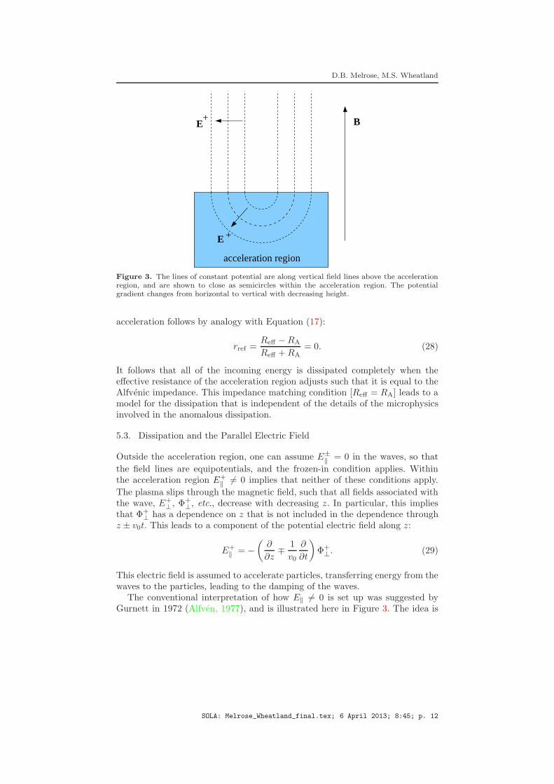
Figure 3. The lines of constant potential are along vertical field lines above the accelerationregion, and are shown to close as semicircles within the acceleration region. The potentialgradient changes from horizontal to vertical with decreasing height.

acceleration follows by analogy with Equation (17):

rref =Reff −RA

Reff +RA

= 0. (28)

It follows that all of the incoming energy is dissipated completely when theeffective resistance of the acceleration region adjusts such that it is equal to theAlfvenic impedance. This impedance matching condition [Reff = RA] leads to amodel for the dissipation that is independent of the details of the microphysicsinvolved in the anomalous dissipation.

5.3. Dissipation and the Parallel Electric Field

Outside the acceleration region, one can assume E±‖ = 0 in the waves, so that

the field lines are equipotentials, and the frozen-in condition applies. Withinthe acceleration region E+

‖ 6= 0 implies that neither of these conditions apply.

The plasma slips through the magnetic field, such that all fields associated withthe wave, E+

⊥ , Φ+⊥, etc., decrease with decreasing z. In particular, this implies

that Φ+⊥ has a dependence on z that is not included in the dependence through

z ± v0t. This leads to a component of the potential electric field along z:

E+‖ = −

(

∂

∂z∓

1

v0

∂

∂t

)

Φ+⊥. (29)

This electric field is assumed to accelerate particles, transferring energy from thewaves to the particles, leading to the damping of the waves.

The conventional interpretation of how E‖ 6= 0 is set up was suggested byGurnett in 1972 (Alfven, 1977), and is illustrated here in Figure 3. The idea is

SOLA: Melrose_Wheatland_final.tex; 6 April 2013; 8:45; p. 12

Alfven Waves in Solar Flares

that the equipotential surfaces, which are along field lines above the accelerationregion, must close across field lines within the acceleration region. Then E+

‖ is

attributed to the normal to equipotential surfaces having a component alongfield lines. A physical argument is that the equipotential surfaces must closeabove a perfectly conducting boundary, and that the fluid velocity associatedwith the waves must go to zero above the line-tied boundary; that is, both E⊥

and u⊥ must go to zero above the photosphere. The following analytic modelillustrates how this leads to E‖ 6= 0.

In a cylindrical model, above the acceleration region the field lines are equipo-tentials, so that Φ± depends only on r and z±v0t. Within the acceleration region,it is assumed that the equipotential surfaces close across the field lines. Supposethe acceleration region is at z < zt. The shape of an equipotential surface atz < zt can be described as a function of r, z. Let the potential surfaces bedescribed by the equation Φ(r, z) − Φ0 = f(r, z) = 0, where different surfacesdepend (implicitly) on a constant rt, that is the value of r at z ≥ zt. The ratio ofthe parallel and perpendicular components is then determined by the functionf(r, z):

E+‖ : E+

⊥ =∂f(r, z)

∂z:∂f(r, z)

∂r. (30)

The lower boundary of the acceleration region is the surface f(r, z) = 0 forrt = R, where rt = R is the boundary of the cylinder at z = zt. A particlethat passes through the acceleration region along a given field line at radius r isaccelerated through a potential difference

∆Φ+ = |Φ+(R)− Φ+(r)|, (31)

where the right hand side is to be evaluated at z ≥ zt.A specific model for the surfaces is to assume that they are elliptical. One has

vertical equipotential surfaces [r = rt < R, for z > zt] and elliptical surfaces,

f(r, z) = r2 + α2(zt − z)2 − r2t = 0, (32)

for z < zt, with α the ratio of the semi-axes of the ellipse. The case α = 1corresponds to semi-circular surfaces illustrated in Figure 3. The lower boundaryof the acceleration region is the surface r2 + α2(zt − z)2 − R2 = 0. The ratioEquation (30) becomes

E+‖ : E+

⊥ = α2(z − zt) : r. (33)

The boundary condition Equation (19) implies that both E+‖ and E+

⊥ vanish on

(and below) the lower boundary of the acceleration region.While plausible, this model is heuristic. The assumptions made is writing

down the wave solution Equation (7) and introducing the wave potential Equa-tion (8) are not valid for E‖ 6= 0.

SOLA: Melrose_Wheatland_final.tex; 6 April 2013; 8:45; p. 13

D.B. Melrose, M.S. Wheatland

6. Discussion

The three features of the Alfven wave model emphasized here are energy trans-port, the mapping of potential differences, and the setting up of intrinsically newcurrent loops involving FACs. In this section, the cylindrical and planar modelsdescribed in Section 4 are used to illustrate these features.

6.1. Alfvenic Energy Transport

Energy transport by Alfven waves is well understood: energy propagates atv0 ≈ vA along the direction of the background magnetic field. Such energypropagation has been invoked in several different flare models. For example,Piddington (1974) developed a model in which the Alfven waves transport theenergy into the corona from below the photosphere during the flare. In the flaremodel due to Fletcher, and Hudson (2008), and in the model developed here,energy already stored in the corona is converted into an Aflvenic energy fluxin a generator region, is transported downwards, and is transferred to energeticelectrons in an acceleration region.

In the Alfven wave model, the energy transport is closely linked to the FAC[J‖] in the waves. It is of interest to compare the present model for energy trans-port with an earlier model (Melrose, 2012b) in which, prior to the flare, the FACprofile in a cylindrical flux tube is described by a function j1(ξ), with ξ = r/R.This profile changes, to j2(ξ), after passage of an Alfvenic front launched by theonset of the flare. It was found that power transported increases with increasingconcentration of j2(ξ) towards ξ = 0; this increase continues as the central con-centration of j2(ξ) increases to arbitrarily large values, compensated by a returncurrent flowing at larger radii. In the present model, the pre-flare FAC is excludedby the assumption that the field lines are straight. This may be interpreted asassuming that the guiding magnetic field is arbitrarily strong, and that both thepre-flare FAC and the FAC in the Alfven waves may be treated as (independent)perturbations. The Alfven wave model then has the same qualitative and semi-quantitative features as in the earlier model. Specifically, in the cylindrical case,the power transported by the Alfven waves increases as J±

‖ becomes increasingly

concentrated towards the axis of the cylinder, where it enhances the pre-flareFAC, with J±

‖ in the opposite direction to the pre-flare FAC at larger radii. In

particular, for the model Equation (20) both the concentration of the FAC andthe energy flux increase with increasing power-law index b. The planar modelEquation (23) has similar properties, with the power-law index d the counterpartof b in the cylindrical model.

6.2. Transport of Potential

A new feature of the Alfven wave model in the solar context is the transportof potential. The Alfven waves are launched in the generator region, where thepower released is due to a cross-field potential and a cross-field current: thecross-field potential in the wave matches that at the boundary of the generatorregion, and the FAC in the wave arises from redirection of the cross-field current

SOLA: Melrose_Wheatland_final.tex; 6 April 2013; 8:45; p. 14

Alfven Waves in Solar Flares

generator

anomalous conductivity

photosphere

Figure 4. The model envisaged here has the generator region at the top, with a total potentialΦ and cross-field current I, below which is an energy transport region to an acceleration regionwith anomalous conductivity. The cross-field current is redirected along field lines to close ina conducting boundary, which is assumed to be the photosphere. Following Holman (1985),the current [I] is assumed to flow up and down multiple [M ] times, forming a picket-fencestructure. The potential across the acceleration region is ∆Φ = Φ/M .

at the boundary of the generator region. Which of these two boundary conditionsdominates determines whether the generator can be approximated as constant-voltage or constant-current, which in turn depends on the ratio of the internaland external impedances. The Alfven waves transport the potential along fieldlines to the acceleration region. Reflection of the Alfven waves from both regionsmodifies the potential, providing a feedback that regulates the rate of dissipationin the acceleration region and the rate of energy release in the generator region.

A realistic theory requires a physical model to determine the form of the wavepotential. Here, simple analytical models are chosen to satisfy the boundarycondition Equation (19) at the edge of the flux tube within which the Alfvenwaves are confined. The magnitude of the potential is not constrained by thetheory, but it is implausible that the total potential available [Φtot = 109 −1010V] can be transported by a single Alfven wave. There is no evidence thatΦtot appears across the acceleration region; the evidence is that the potentialthat does appear across the acceleration region is ∆Φ = Φtot/M , with M oforder 106.

The explanation for the multiplicity [M ] proposed by Holman (1985) can beincorporated into the model. Holman’s suggestion is that there are M pairs ofup and down current channels, leading to the “picket-fence” model illustrated inFigure 4. One requires that the potential across the acceleration region [∆Φ =

SOLA: Melrose_Wheatland_final.tex; 6 April 2013; 8:45; p. 15

D.B. Melrose, M.S. Wheatland

Φtot/M ] be of order 104V for each channel, each of which has up and downcurrents [∆I] of order I. It is unrealistic to use cylindrical geometry to describemultiple pairs of up and down currents, which would occur in alternate concentricrings. In a planar geometry, the pairs of up and down current are in alternatecurrent sheets. A more realistic geometry requires an arrangement for the Mcurrent pairs, in either cylindrical (r, φ) or cartesian (x, y) geometry, combinedwith a model for each of the current pairs.

A physical explanation is needed for the multiplicity [M ] of current pairs.One possibility is to consider restrictions imposed by the microphysics on thepotential in the Alfven waves. If the potential is restricted to Φ+ . 104V,then M = 106 current channels must develop in order to provide the requiredtotal rate of energy loss. Moreover, these current channels must develop si-multaneously; if they develop sequentially, the implied timescale of 106 Alfvenpropagation times greatly exceeds the timescale of a flare. These problems arenot discussed further here.

6.3. Dissipation and Acceleration

How Alfven waves damp and accelerate particles effectively is an unsolved prob-lem. Some form of anomalous dissipation is required. As has long been recog-nized, a requirement for a current-driven instability is a very high current density,which implies filamentation of the current into many high-current-density chan-nels (Holman, 1985; Tsuneta, 1985; Melrose, and McClymont, 1987; Melrose,1990; Emslie, and Henoux, 1995; Tsuneta, 1995). Let the current thresholdfor instability be Jcrit. Suppose each filament is cylindrical, and of radius λ,such that the current in each filament is If = πλ2Jcrit. One requires a largenumber [Nf = I/If ] of such channels. For a specific model, Haerendel (2012)estimated Jcrit = 4× 103Am−2 and λ = 1meter. An unavoidable implication isthat anomalous dissipation requires that the dissipation region is highly struc-tured, involving very small scales perpendicular to the field lines. The followingargument based on the Alfven wave model leads to a similar conclusion.

Suppose one balances the incoming Poynting vector in the Alfven waves withthe outgoing kinetic energy flux in accelerated electrons with a number densityne. This gives

1

µ0v0

(

dΦ+(r)

dr

)2

= ne

(

2

m

)1/2

[e∆Φ+(r)]3/2, (34)

with ∆Φ+(r) given by Equation (31), and where [2e∆Φ+(r)/m]1/2 is the speedof the accelerated electrons. Using Equation (31), one may integrate Equation(34) to find

e∆Φ+(r) = 2mv20

( r

λ

)4

,1

λ=

ωp

4c, (35)

and use Equation (16) to find

|J+‖ | = enev0

3

2

( r

λ

)2

. (36)

SOLA: Melrose_Wheatland_final.tex; 6 April 2013; 8:45; p. 16

Alfven Waves in Solar Flares

With e∆Φ+(r) of order 103 × mv20 under coronal conditions, it follows fromEquation (35) that the model requires perpendicular structure in Φ+(r) on ascale of a few tens of skin depths [c/ωp] which is of the same order of magnitudeas the λ estimated by Haerendel (2012) by a different argument. It follows fromEquation (36) that there is a high current density, sufficient to trigger anomalousconductivity, on the scale λ.

The result, Equation (36), demonstrates an inconsistency in the Alfven model,as developed here. The Alfven wave model applies on a macro scale, plausiblydescribing the energy and potential transport to the top of the accelerationregion. Effective dissipation involves micro-scale structures, and these must betaken into account within the dissipation region. The model developed here forthe dissipation region can at best be regarded as applying to properties averagedover a statistically large distribution of such micro-scale structures.

6.4. Return Current

The long-standing “number problem” can be partly resolved by requiring a re-turn current between denser regions of the solar atmosphere and the accelerationregion. Existing models for the return current have invoked both electrostaticand inductive effects (Brown, and Bingham, 1984; Spicer, and Sudan, 1984; vanden Oord, 1990). The Alfven wave model provides a new way of modeling thereturn current, in terms of Alfven waves setting up new current loops, thatclose across field lines in the acceleration region and in denser regions of thesolar atmosphere. Such a model has an important qualitative difference fromthese earlier models, in which the ions were neglected (van den Oord, 1990).Neglecting the ions leads to neglecting the polarization current, so that theinductive effects propagate effectively at the speed of light. It is essential toinclude the polarization current, and then Equation (3) implies that inductiveeffects are transported along field lines by Alfven waves at the MHD speed. AnAlfven wave model for an inductively driven return current is needed to showhow the electrons are continuously resupplied to the acceleration region, as isnecessary for both “first phase” electron acceleration and for auroral electronacceleration (Marklund, 2009).

7. Conclusion

The main point of this article is that large-amplitude Alfven waves play animportant role in solar flare physics. These are not “waves” in the conventionalsense, with a well-defined frequency and wave vector, but are specific solutionsof the Alfven wave equation Equation (6) involving a cross-field wave potential[Φ±

⊥] and field aligned currents, J±‖ , determined by the wave potential. Energy

transport is along field lines at the MHD speed [v0 ≈ vA] as for any (torsional)Alfven wave. The wave potential provides the mapping of the potential imposedin the generator region onto the acceleration region. Reflected Alfven wavestransport the reaction (of the acceleration region or the photosphere) back tothe generator region, providing a coupling between them. The Alfven waves set

SOLA: Melrose_Wheatland_final.tex; 6 April 2013; 8:45; p. 17

D.B. Melrose, M.S. Wheatland

up new closed current loops, with oppositely directed FACs closing across fieldlines at the two ends (in the generator region and the photosphere).

A long-standing problem with models involving particle acceleration by Alfvenwaves is the mechanism that allows the Alfven waves to damp and to transfertheir energy to particles. The interpretation of the wave amplitude in termsof a cross-field potential provides a way of interpreting this damping withoutidentifying the microphysics involved. Within the acceleration region it is as-sumed that the wave amplitude, and hence the cross-field potential, decreasesdownwards. There is then a nonzero gradient of the potential along the field linesimplying a nonzero E‖. This E‖ accelerates the particles. In an idealized model,the Alfvenic energy flux at the top of the acceleration region is converted intoa kinetic-energy flux in accelerated electrons at the bottom of the accelerationregion, where the wave amplitude (potential) is zero. The rate of dissipation canbe determined by assuming that the anomalous dissipation processes adjust tomaximize the power dissipated. This leads to the impedance matching conditionfor the effective resistance, Reff = RA, of the acceleration region. All anomalousdissipation processes involve microphysics on tiny space scales, of order one meterin the present context (Haerendel, 2012), and the relation between processes onmicro and macro scales is treated heuristically here. This relation needs to beexplained in a more detailed model.

The Alfven wave model indicates how long-standing, unsolved problems re-lated to bulk energization of electrons may be resolved. It is assumed that theacceleration results from E‖ 6= 0 in an acceleration region, along field linesabove a hard X-ray source in the chromosphere. One problem is the seeminginconsistency between the large cross-field potential, of order 1010Volts, and theenergy, e∆Φ of order 104 eV, of the accelerated electrons. One way of resolvingthis (Holman, 1985) is to assume that the pre-flare current flows back and forthbetween the generator and dissipation regions many (M = 106) times. Electronsare accelerated downward in a sequence of M jumps in potential, one jumpfor each instance of I flows up through the acceleration region. The additionalinsight that the Alfven wave model provides is that M current paths may beregarded asM closed current loops set up by Alfven waves. The number problemis resolved by identifying the total rate [N ] that electrons precipitate as M timesthe rate [I/e] for each of these loops. However, there is no obvious explanationwithin the model for the value of the multiplicity [M ]. A speculation is that themicrophysics in the acceleration region constrains the value of e∆Φ.

There are unsolved problems related to the acceleration region (Haerendel,2012). In particular, the self-consistency argument for E‖ 6= 0, based on thedamping of the waves due to energy transfer to particles by E‖, is heuristic, andneeds to be complemented by a specific mechanism that accounts for E‖ 6= 0. Allsuch mechanisms appear to involve very small scales perpendicular to the fieldlines, estimated to be of order one meter by Haerendel (2012). An outstandingproblem is how this microphysics relates to the macroscopic model discussed inthis article.

The Alfven wave model developed here is highly simplified, and is appliedspecifically only to transport of energy between the generator and accelerationregion. However, the physics involved is likely to be widely relevant to energytransport and energy release in the solar atmosphere.

SOLA: Melrose_Wheatland_final.tex; 6 April 2013; 8:45; p. 18

Alfven Waves in Solar Flares

Appendix

A. Response of a Plasma at Low Frequencies

The response of a cold plasma may be described by the dielectric tensor Kij(ω)(Stix, 1962):

Di(ω) = ε0Kij(ω)Ej(ω), Kij(ω) =

S −iD 0iD S 00 0 P

. (37)

At sufficiently low frequencies, when dissipation is neglected, one has

S ≈ 1 +c2

v2A, D ≈ 0, P = 1−

ω2p

ω2. (38)

The electric induction [D] includes the response of the plasma through thepolarization [P]:

D = ε0E+P, ρind = −∇ ·P, Jind =∂P

∂t, (39)

where ρind and Jind are the induced charge and current densities. The perpen-dicular component of the response is

P⊥ =c2

v2Aε0E⊥. (40)

The temporal derivative of Equation (40) gives

Jind⊥ =c2

v2Aε0

∂E⊥

∂t, (41)

which reproduces Equation (3). The parallel term in the low-frequency, cold-plasma limit gives

∂Jind‖

∂t= ε0ω

2pE‖. (42)

The components Equation (41) and Equation (42) of the current density areincluded in Maxwell’s equations. For the perpendicular components, one obtains

(

1

v20

∂2

∂t2−∇2

)

E⊥ = −∇⊥ρext

ε0− µ0

∂Jext⊥

∂t, (43)

where the right hand side includes source terms. The result Equation (43) re-produces Equation (6) when the source terms are neglected. For the parallelcomponent, one obtains

[

1

c2∂2

∂t2+

ω2p

c2−∇2

]

E‖ = −1

ε0

∂ρext∂z

− µ0

∂Jext‖

∂t. (44)

SOLA: Melrose_Wheatland_final.tex; 6 April 2013; 8:45; p. 19

D.B. Melrose, M.S. Wheatland

References

Alfven, H.: 1977, Rev. Geophys. Space Phys. 15, 271.ADS:1977RvGSP..15..271A, doi:10.1029/RG015i003p00271.

Alfven, H., Carlqvist, P.: 1967, Solar Phys. 1, 220.ADS:1967SoPh....1..220A, doi:10.1007/BF00150857.

Bian, N.H., Kontar, E.P., Brown, J.C.: 2010, Astron. Astrophys. 519, A114.ADS:2010A&A...519A.114B, doi:10.1051/0004-6361/201014048.

Borovsky, J.E.: 1993, J. Geophys. Res. 98, 6101.ADS:1993JGR....98.6101B, doi:10.1029/92JA02242.

Brown, J.C., Bingham, R.: 1984, Astron. Astrophys. 508, 993.ADS:1984A&A...131L..11B.

Colgate, S.A. 1978, Astrophys. J. 221, 1068.ADS:1978ApJ...221.1068C, doi:10.1086/156111.

Dorogovtsev, S.N., Mendez, J.F.F.: 2002, Adv. Phys. 51, 1079.doi:10.1080/00018730110112519.

Emslie, A.G., Henoux, J.C.: 1995, Astrophys. J. 446, 371.ADS:1995ApJ...446..371E, doi:10.1086/175796.

Fletcher, L., Hudson, H.S.: 2008, Astrophys. J. 675, 1645.ADS:2008ApJ...675.1645F, doi:10.1086/527044.

Haerendel, G.: 1994, Astrophys. J. Suppl. 90, 765.ADS:1994ApJS...90..765H, doi:10.1086/191901.

Haerendel, G.: 2001, Phys. Plasmas 8, 2365.ADS:2001PhPl....8.2365H, doi:10.1063/1.1342227.

Haerendel, G.: 2009, Astrophys. J. 707, 903.ADS:2009ApJ...707..903H, doi:10.1088/0004-637X/707/2/903.

Haerendel, G.: 2012, Astrophys. J. 749, 166.ADS:2012ApJ...749..166H, doi:10.1088/0004-637X/749/2/166.

Holman, G.D.: 1985, Astrophys. J. 293, 584.ADS:1985ApJ...293..584H, doi:10.1086/163263.

Hoyng, P., Brown, J.C., Van Beek, H.F.: 1976, Solar Phys. 48, 197.ADS:1976SoPh...48..197H, doi:10.1007/BF00151992.

Litvinenko, Yu.E., Somov, B.V.: 1991, Solar Phys. 131, 319.ADS:1991SoPh..131..319L, doi:10.1007/BF00151641.

Lysak, R.L.: 1985, J. Geophys. Res. 90, 4178.ADS:1985JGR....90.4178L, doi:10.1029/JA090iA05p04178.

MacKinnon, A.L. Brown, J.C.: 1989, Solar Phys. 122, 303.ADS:1989SoPh..122..303M, doi:10.1007/BF00912997.

McPherron, R.L., Russel, C.T., Aubry, M.P.: 1973, J. Geophys. Res. 78, 3131.ADS:1973JGR....78.3131M, doi:10.1029/JA078i016p03131.

Marklund, G.T.: 2009, Space Sci. Rev. 142, 1.ADS:2009SSRv..142....1M, doi:10.1007/s11214-008-9373-9.

Melrose, D.B.: 1990, Solar Phys. 130, 3.ADS:1990SoPh..130....3M, doi:10.1007/BF00156775.

Melrose, D.B.: 2012a, Astrophys. J. 749, 58M.ADS:2012ApJ...749...58M, doi:10.1088/0004-637X/749/1/58.

Melrose, D.B.: 2012b, Astrophys. J. 749, 59M.ADS:2012ApJ...749...59M, doi:10.1088/0004-637X/749/1/59.

Melrose, D.B., McClymont, A.N.: 1987, Solar Phys. 113, 241.ADS:1982SoPh..113..241M, doi:10.1007/BF00147704.

Northrop, T.G.,: 1963, Adiabatic Motion of Charged Particles, Wiley.doi:10.1029/RG001i003p00283.

Paschmann, G., Haaland, S., Treumann, R.: 2002, Space Sci. Rev. 103, 1.ADS:2002SSRv..103C....P, doi:10.1023/A:1023030716698.

Piddington, J.H.: 1974, Solar Phys. 38, 465.ADS:1974SoPh...38..465P, doi:10.1007/BF00155082.

Raadu, M.A.: 1989, Phys. Rep. 178, 25ADS:1989PhR...178...25R, doi:10.1016/0370-1573(89)90109-9.

Scholer, M.: 1970, Planet. Space Sci. 18, 977.ADS:1970P&SS...18..977S, doi:10.1016/0032-0633(70)90101-7.

SOLA: Melrose_Wheatland_final.tex; 6 April 2013; 8:45; p. 20

Alfven Waves in Solar Flares

Simon, A.: 1955, Phys. Rev. 98, 317.ADS:1955PhRv...98..317S, doi:10.1103/PhysRev.98.317.

Song, Y., Lysak, R.L.: 2006, Phys. Rev. Lett. 96, 145002.ADS:2006PhRvL..96n5002S, doi:10.1103/PhysRevLett.96.145002.

Spicer, D.S., Sudan, R.N.: 1984, Astrophys. J. 280, 448.ADS:1984ApJ...280..448S, doi:10.1086/162011.

Stix, T.H.: 1962, The Theory of Plasma Waves, McGraw-Hill.ADS:1962tpw..book.....S.

Tsuneta, S.: 1985, Astrophys. J. 290, 353.ADS:1985ApJ...290..353T, doi:10.1086/162992.

Tsuneta, S.: 1995, Pub. Astron. Soc. Japan 47, 691.ADS:1995PASJ...47..691T.

van den Oord, G.H.J.: 1990, Astron. Astrophys. 243, 496.ADS:1990A&A...234..496V.

Vogt, J., Haerendel, G.: 1998, Geophys. Res. Lett., 25, 277.ADS:1998GeoRL..25..277V, doi:10.1029/97GL53714.

Vogt, J., Haerendel, G., Glassmeier, K.H.: 1999 J. Geophys. Res. 104, 269.ADS:1999JGR...104..269V, doi:10.1029/1998JA900048.

Wild, J.P., Smerd, S.F., Weiss, A.A.: 1963, Ann. Rev. Astron. Astrophys. 1, 291.ADS:1963ARA&A...1..291W, doi:10.1146/annurev.aa.01.090163.001451.

SOLA: Melrose_Wheatland_final.tex; 6 April 2013; 8:45; p. 21

SOLA: Melrose_Wheatland_final.tex; 6 April 2013; 8:45; p. 22