transformation of p-s to p-p seismic data of p-s to p-p seismic data crewes research report –...

Transformation of P-S to P-P seismic data

CREWES Research Report – Volume 8 (1996) 18-1


Wai-kin Chan and Robert R. Stewart

ABSTRACT

Conventional converted-wave processing requires special algorithms to account forthe P-S asymmetric move-out in the CMP domain. Two techniques, asymmetric move-out correction (ASMO) and average Vp/Vs value analysis by simulated annealing areproposed to correct for this asymmetric move-out behavior and transform the P-S datainto P-P, so that normal P-wave processing algorithms can be followed. The syntheticexample presented here shows some promising results.

INTRODUCTION

A more complete recording of the seismic experiment requires measurement of threecomponents of the received waves. From these 3-C measurements we can attempt toimprove P-wave sections and create independent converted-wave (P-S) images. Jointlyinterpreting P-P and P-S sections can significantly improve the description of the geo-logical section and reservoir rocks. To facilitate this ultimate interpretation though, weneed to make P-S data easily correlative to P-P data. To do this, we would like to haveboth sections in P-P time (or depth). We would also like to be able to use the existingtools of P-P processing and have this whole procedure take minimal time.

We propose to solve these problems by transforming P-S data to P-P times.This willreposition the P-S data (with their asymmetric ray paths and gathers) to look like sym-metric P-P data. We can then use many of the efficient conventional processes such asCMP binning and DMO. This technique is based on a new asymmetric movout correc-tion (ASMO) and Vp/Vs value analysis.

THEORY OF ASMO

The method of the ASMO starts from the downward continuation of the receivedwavefield, with P-wave velocity, to a depth increment. The P-wave travel-times fromthe shot to the depth points are calculated. The time samples of the downward continu-ation wavefield that corresponding to the calculated travel-times are then upward con-tinued with S-wave velocity. This procedure is repeated for all depth increments andthe output of the transformation is the summation of all the upward continuation of S-wavefield. Let S(x,z=0,t) denote the recorded P-S shot gather at the Earth’s surface,then the corresponding pseudo P-P shot gather, P(x,z=0,t) is given by

(1)

where is the upward continuation operator from z to the surface with Vsvelocity,

is the downward continuation operator from the surface to z with Vp velocity

td is the P-wave travel-times from the shot to the depth points (x,z),

is the Dirac delta function.

In essence, the receivers are downward continued with S-wave velocity field to a cer-

P x 0 t, ,( ) U zvs Dz

vp S x 0 t, ,( )[ ] δ t td x y,( )–( )[ ]z

∑=

Dzvp

Uzvs

δ

Chan and Stewart

18-2 CREWES Research Report – Volume 8 (1996)

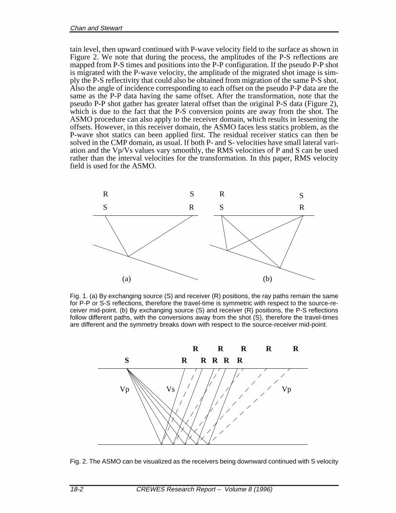
tain level, then upward continued with P-wave velocity field to the surface as shown inFigure 2. We note that during the process, the amplitudes of the P-S reflections aremapped from P-S times and positions into the P-P configuration. If the pseudo P-P shotis migrated with the P-wave velocity, the amplitude of the migrated shot image is sim-ply the P-S reflectivity that could also be obtained from migration of the same P-S shot.Also the angle of incidence corresponding to each offset on the pseudo P-P data are thesame as the P-P data having the same offset. After the transformation, note that thepseudo P-P shot gather has greater lateral offset than the original P-S data (Figure 2),which is due to the fact that the P-S conversion points are away from the shot. TheASMO procedure can also apply to the receiver domain, which results in lessening theoffsets. However, in this receiver domain, the ASMO faces less statics problem, as theP-wave shot statics can been applied first. The residual receiver statics can then besolved in the CMP domain, as usual. If both P- and S- velocities have small lateral vari-ation and the Vp/Vs values vary smoothly, the RMS velocities of P and S can be usedrather than the interval velocities for the transformation. In this paper, RMS velocityfield is used for the ASMO.

Fig. 1. (a) By exchanging source (S) and receiver (R) positions, the ray paths remain the samefor P-P or S-S reflections, therefore the travel-time is symmetric with respect to the source-re-ceiver mid-point. (b) By exchanging source (S) and receiver (R) positions, the P-S reflectionsfollow different paths, with the conversions away from the shot (S), therefore the travel-timesare different and the symmetry breaks down with respect to the source-receiver mid-point.

Fig. 2. The ASMO can be visualized as the receivers being downward continued with S velocity

(a) (b)

S R S R

R S R S

S R R R R R

R R R R R

Vp Vs Vp



(Vs) to a certain depth, followed by upward continuation to the surface with P velocity (Vp).

Vp/Vs analysis

In the above method, it is assumed that the background RMS velocities for both Pand S are known. In general, both velocity fields can be extracted from the velocityanalysis during the P-P and the P-S processing. However, if after the transformation,the events on the pseudo P-P data need to be tied with that on the real P-P data, thenthese velocities may not be accurate enough. Consider a simple uniform layer, shownin Figure 3, 3 km thick and with Vp = 3000 m/s, Vs = 1500 m/s. The two-way verticalP-P and P-S travel-times for this model are 2 seconds and 3 seconds respectively. As-suming that there is only -3% relative error in the S velocity giving Vs = 1455 m/s andVp/Vs = 2.06. The event at 3 seconds two-way P-S time, now maps to 1.96 secondstwo-way P-P time giving -40 ms in error. If the dominant frequency of the wavelet inthe P-P data is 30 Hz. This 40 ms error translates into more than a dominant wavelengthof the wavelet. We conclude that the average Vp/Vs ratio in depth from the correlationof the events on the P-P and the P-S data, especially for the latter events, is much sen-sitive than the one obtained from the normal velocity analysis, which has more error forthe later events. Therefore, tying the events between P-P and P-S data can provide ex-cellent estimation of the average Vp/Vs ratios and these ratios can be used for the pur-pose of the P-S transformation. In the next section, it will be shown that simulatedannealing technique can be incorporated to correlate events between P-P and P-S auto-matically and to obtain the variable average Vp/Vs ratios in the time and space do-mains. Once these average Vp/Vs ratios are obtained, they can be converted intointerval Vp/Vs ratios, for example by analyzing the P-P and P-S interval times betweena major geological event.

Fig. 3. Consider a 3km thick uniform layer with Vp=3000m/s and Vs=1500ms. The P-P and theP-S two-way vertical travel-times of the model are 2 seconds and 3 seconds respectively. If theevent at 3 seconds P-S time is compressed to P-P time with Vp=3000 m/s and Vs=1455 m/s,the resulted P-P time will be at 1.96 seconds giving -40 ms error.

SIMULATED ANNEALING

Simulated annealing has long been used as a technique to solve global optimizationproblems in geophysics (Rothman, 1985, Sen and Stoffa, 1991, Chunduru et al., 1996,Jervis et al., 1996). Starting from an initial point, the algorithms takes a step and theoptimization function is evaluated. It is different from other optimization techniques,like the nonlinear simplex (Rowan, 1990), that only accepts a favorable solution duringeach step. By accepting non-favorable solutions occasionally, based on Metropolis cri-teria, local optima can be escaped. As the optimization process proceeds, the steplengths decline, the chance of accepting non-favorable solutions decreases, and the al-gorithm closes in on the global optimum.

Correlation of events between P-P and P-S stack traces can be formulated as a global

Vp = 3000 m/s

Vs = 1500 m/s3 km

Chan and Stewart


optimization problem. The functional value to be optimized is the cross-correlation be-tween the reference P-S trace and the stretched P-P trace, based on the current estimatedaverage Vp/Vs values. When the proper Vp/Vs values applied on the stacked traces, thematch between two traces reaches optimum, and hence it gives the largest cross-corre-lation value. This technique assumes that the P-S and P-P reflectivity are well correlat-ed. If this is not true at some locations in time, the Vp/Vs values obtained at theselocations are in error. However as it is the average Vp/Vs value, not the interval Vp/Vsvalue being sought, the errors should be localized.

The number of the average Vp/Vs values used in a trace is important. Fortunately,from the P-wave horizon velocity analysis, several key horizons or events are alreadyidentified in terms of P-wave two-way travel-times, and they can be used as controlpoints for the Vp/Vs analysis. The Vp/Vs values among the control points are just linearinterpolated, and the resulted Vp/Vs values become functions of P-wave travel timesand CDP locations. To further stabilize the solution of the optimization, the match isfirst done on the low frequency version of the P-P and the P-S stack traces. The resultof these Vp/Vs values is used as constrains for the final match between the original P-P and P-S traces.

ALTERNATIVE CONVERTED-WAVE PROCESSING

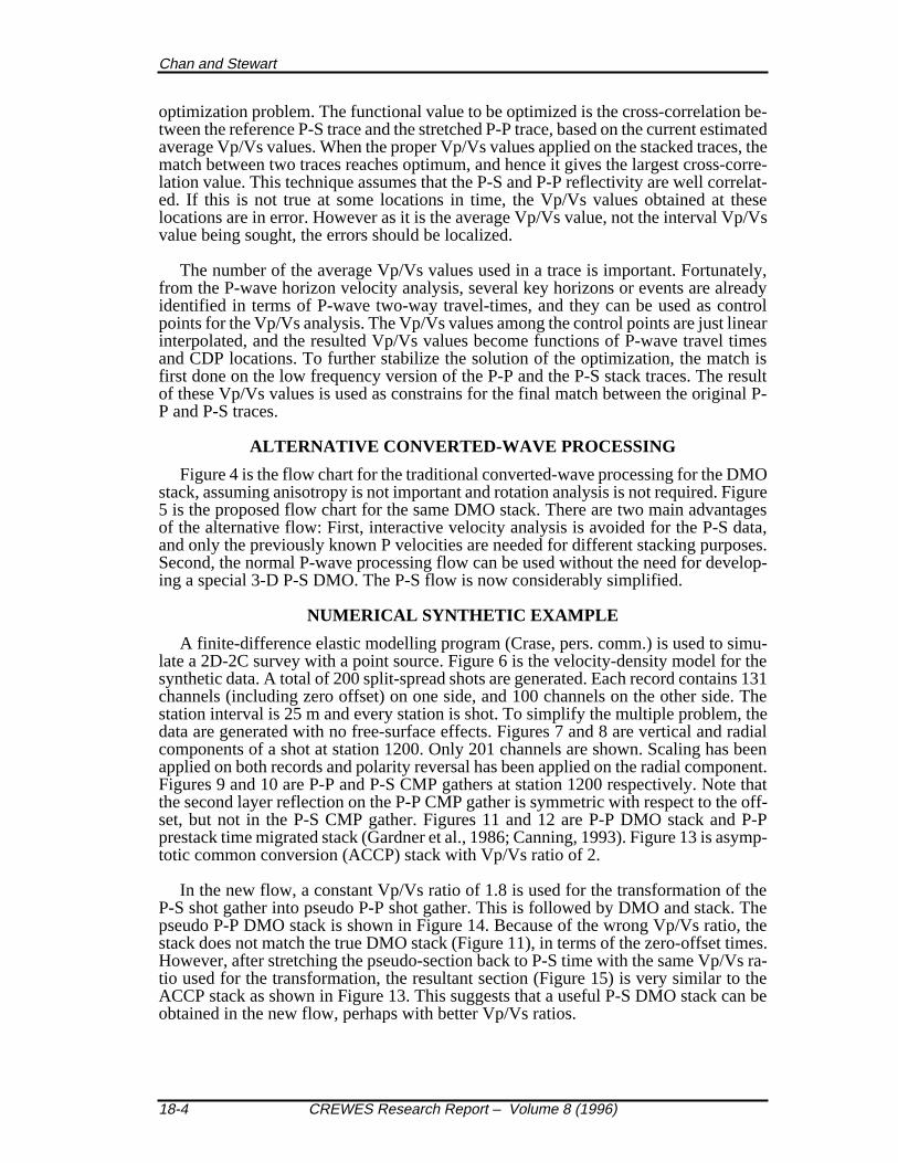
Figure 4 is the flow chart for the traditional converted-wave processing for the DMOstack, assuming anisotropy is not important and rotation analysis is not required. Figure5 is the proposed flow chart for the same DMO stack. There are two main advantagesof the alternative flow: First, interactive velocity analysis is avoided for the P-S data,and only the previously known P velocities are needed for different stacking purposes.Second, the normal P-wave processing flow can be used without the need for develop-ing a special 3-D P-S DMO. The P-S flow is now considerably simplified.

NUMERICAL SYNTHETIC EXAMPLE

A finite-difference elastic modelling program (Crase, pers. comm.) is used to simu-late a 2D-2C survey with a point source. Figure 6 is the velocity-density model for thesynthetic data. A total of 200 split-spread shots are generated. Each record contains 131channels (including zero offset) on one side, and 100 channels on the other side. Thestation interval is 25 m and every station is shot. To simplify the multiple problem, thedata are generated with no free-surface effects. Figures 7 and 8 are vertical and radialcomponents of a shot at station 1200. Only 201 channels are shown. Scaling has beenapplied on both records and polarity reversal has been applied on the radial component.Figures 9 and 10 are P-P and P-S CMP gathers at station 1200 respectively. Note thatthe second layer reflection on the P-P CMP gather is symmetric with respect to the off-set, but not in the P-S CMP gather. Figures 11 and 12 are P-P DMO stack and P-Pprestack time migrated stack (Gardner et al., 1986; Canning, 1993). Figure 13 is asymp-totic common conversion (ACCP) stack with Vp/Vs ratio of 2.

In the new flow, a constant Vp/Vs ratio of 1.8 is used for the transformation of theP-S shot gather into pseudo P-P shot gather. This is followed by DMO and stack. Thepseudo P-P DMO stack is shown in Figure 14. Because of the wrong Vp/Vs ratio, thestack does not match the true DMO stack (Figure 11), in terms of the zero-offset times.However, after stretching the pseudo-section back to P-S time with the same Vp/Vs ra-tio used for the transformation, the resultant section (Figure 15) is very similar to theACCP stack as shown in Figure 13. This suggests that a useful P-S DMO stack can beobtained in the new flow, perhaps with better Vp/Vs ratios.



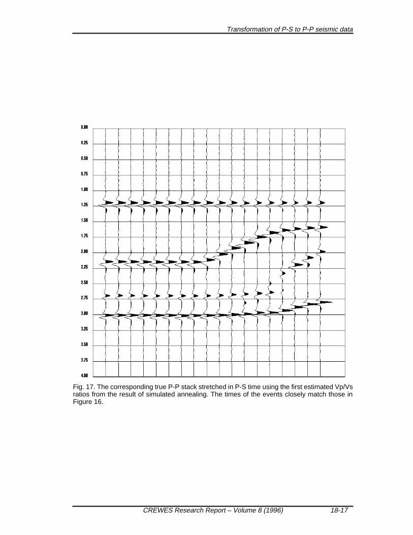
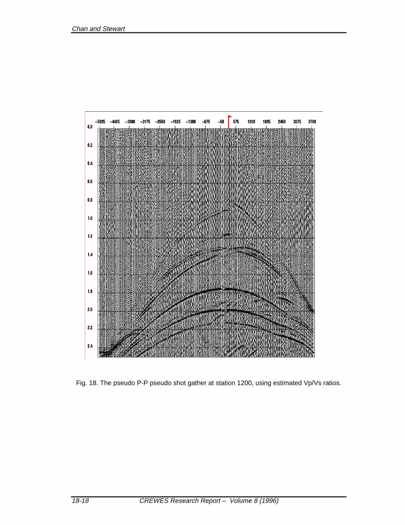
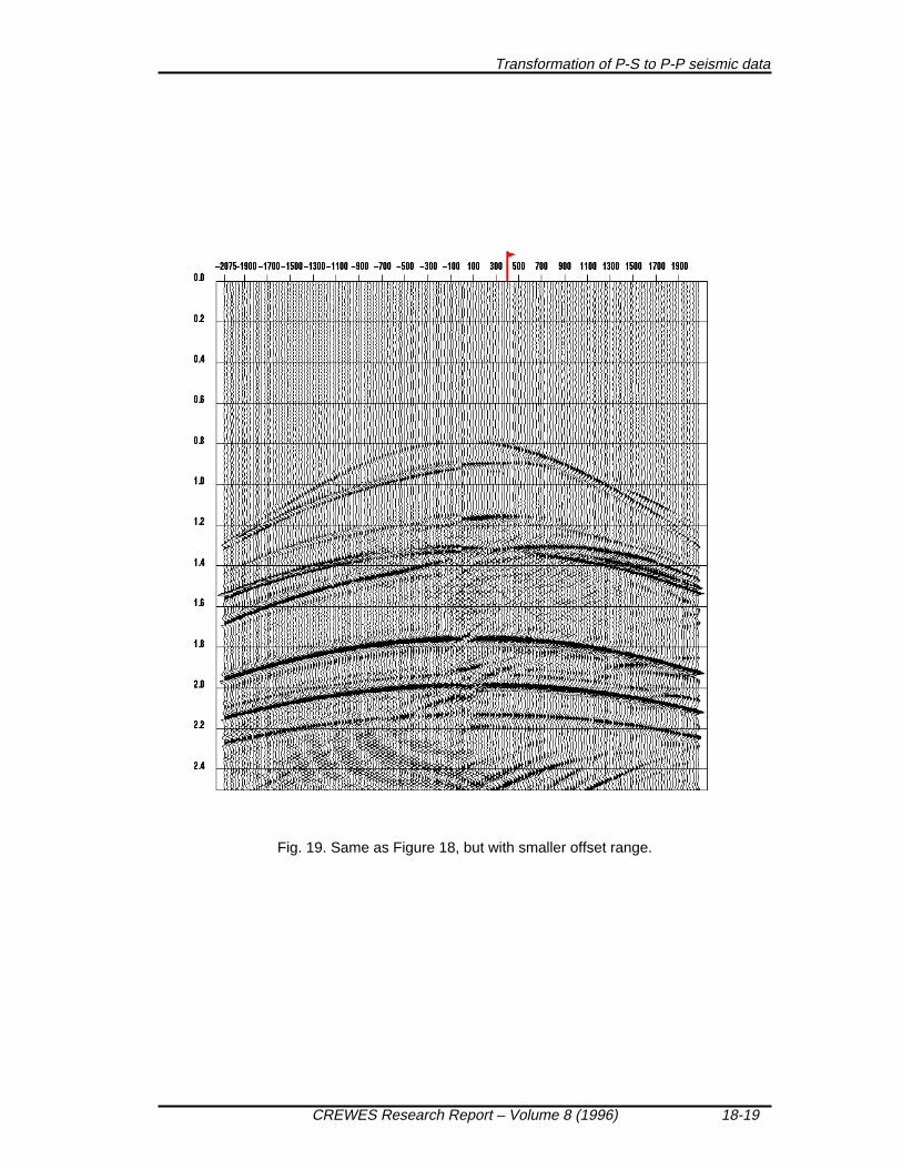
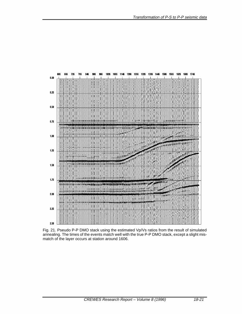
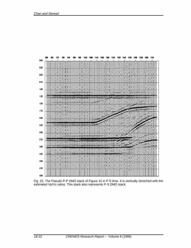
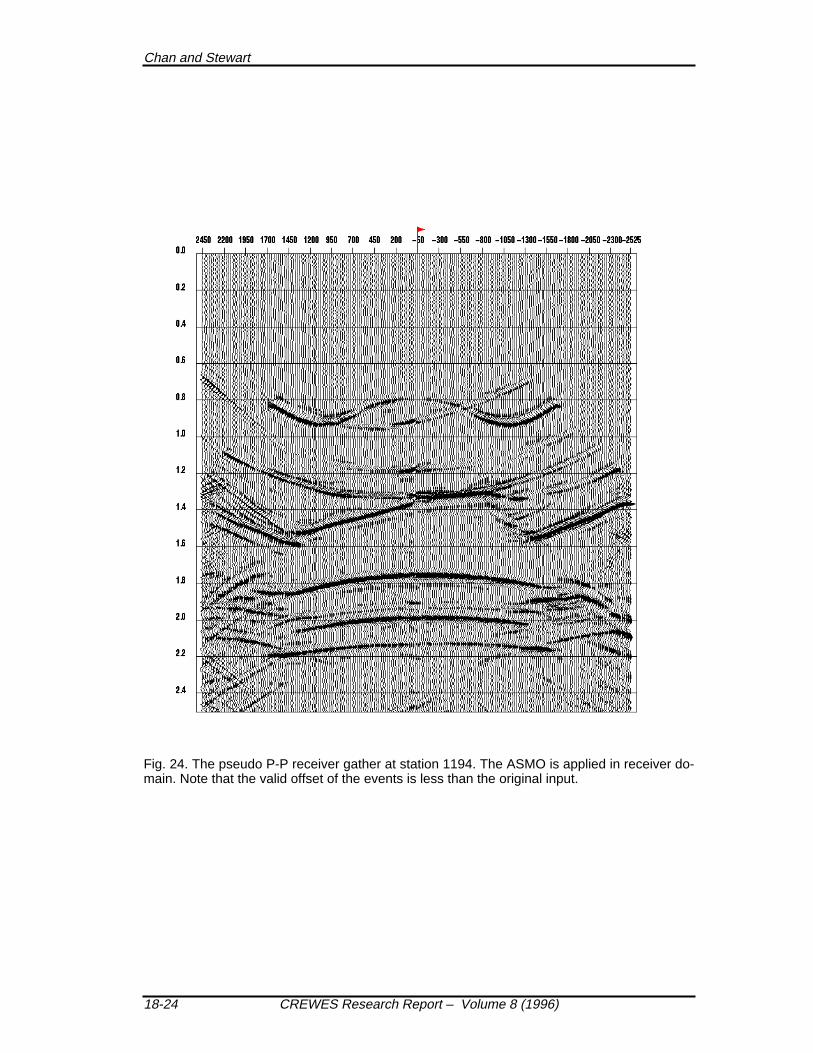
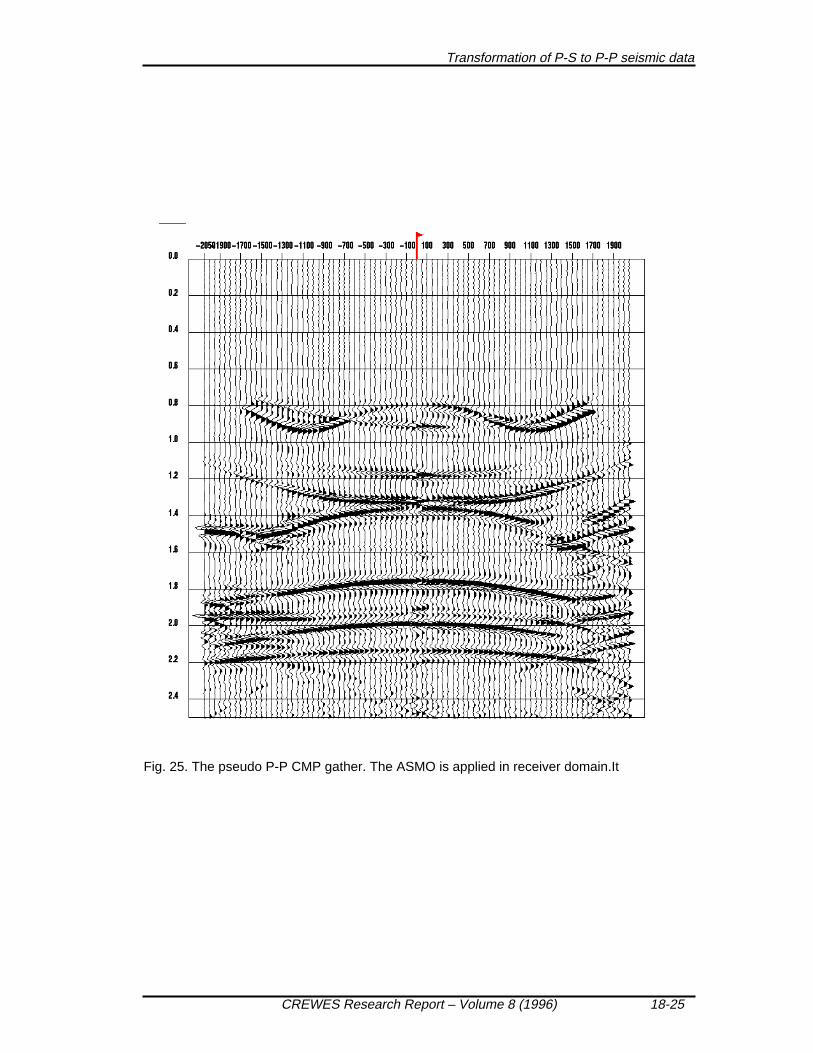
The next step is to use simulated annealing technique to analysis the time and spacevariant Vp/Vs ratios. A selected subset of pseudo P-P DMO stack in P-S time (Figure16) is used for reference traces for the correlation. In Figure 17, the corresponding trueP-P DMO stack traces are stretched with the estimation of Vp/Vs ratios from the corre-lation analysis. Comparing between Figure 16 and Figure 17, it suggested the simulatedannealing does obtain optimum Vp/Vs ratios for the match. These new estimated Vp/Vs ratios are used to update the transformation process. Figure 18 is the updated pseudoP-P shot gather. After the transformation, the largest offset changes from 3250 m toabout 5000 m. Figures 19 and 20 show the limited offsets version of Figure 18 in shotand CMP domains. Figure 21 is the new pseudo P-P DMO stack, and it is in generalagreement with the true P-P DMO stack (Figure 9). There are some mis-ties at aroundstation 1950 for the last layer. The main reason is that the estimated Vp/Vs ratios arealong the normal ray paths and the velocities used for the ASMO are along image raypaths. Because there is significant lateral velocity variation in that region, these two raypaths are different enough to give rise to the error. Figure 22 is the pseudo P-P DMOstack plotted in the P-S time. This also represents the P-S DMO stack. The pseudo P-Pprestack gathers are also migrated with the P-P algorithm and the stack is shown in Fig-ure 23. The receiver version of the ASMO was also tested. Figures 24 and 25 are thereceiver gather at station 1194 and CMP gather at station 1200. The resultant pseudo P-P DMO stack is shown in Figure 26. It is similar to Figure 21, but it is nosier, especiallyon the top. This is due to the loss of offset after ASMO. This suggests that a top mutemay be necessary after the receiver ASMO.

P-wave shot staticsResidual receiver statics

CCP binning with assumed Vp/Vs ratiosVelocity analysis on CCPNMO correction on CCP

P-S DMO on common offset planesRemove NMO

Velocity analysis on CCPCCP re-gathering with proper Vp/Vs ratios and velocity analysis (optional)

NMO correction on CCPP-S DMO on common offset planes

Stack

Fig. 4. The flow chart for the traditional converted-wave DMO stack.

P-wave shot staticsResidual receiver statics

P-S to P-P transformationDMO

Velocity analysisStack

Fig. 5. The alternative flow chart for the converted-wave DMO stack

Chan and Stewart


CONCLUSIONS

Two new techniques, ASMO and Vp/Vs analysis using simulated annealing havebeen discussed. It has been shown that these two techniques can be used together totransform the P-S data into P-P time and form an alternative processing flow for con-verted-waves. This eliminates the need for the P-S velocity analysis, and normal P-Pprocessing algorithms can be followed. These techniques can be easily extended to 3-D geometries and special 3-D processing algorithms for P-S data, like 3-D P-S DMOcan be avoided.

REFERENCES

Canning A., 1993, Organization and imaging of three-dimensional seismic reflection data before stack:Ph.D. thesis, Rice University.

Chunduru, R. K., Sen, M. K., and Stoffa, P. L., 1996, 2-D resistivity inversion using spline parameter-ization and simulated annealing: Geophysics, 61, 151-161.

Gardner, G. H. F., Wang, S. Y., Pan, N. D., and Zhang, Z., 1986, Dip-moveout and prestack imaging:Ann. Mtg. Offshore Tech. Conf., Expanded Abstracts, Vol. 2, 75-81.

Jervis, M., Sen, M. K., and Stoffa, P. L., 1996, Prestack migration velocity estimation using nonlinearmethods: Geophysics, 61, 138-150.

Rowan, T., 1990, Functional stability analysis of numerical algorithms: Ph.D. thesis, Department ofComputer Sciences, University of Texas at Austin.

Rothman, D. H., 1985, Nonlinear inversion, statistical mechanics, and residual statics estimation: Geo-physics, 50, 2784-2796.

Sen, M. K., and Stoffa, P. L., 1991, Nonlinear one-dimensional seismic wave form inversion using sim-ulated annealing: Geophysics, 56, 1624-1638.

Fig. 6. Velocity-density depth model of the numerical synthetic example.

606 942 1278 1614 1950 22860.0

0.8

1.6

2.4

3.2

Vp=2000 m/s density=1.000g/cm3

Vs=1000 m/s Vp/Vs = 2.000


Vs=1250 m/s

Vp/Vs = 2.000


Vs=1360 m/s Vp/Vs = 2.206Vp=3500 m/s


Vs=2363 m/s Vp/Vs = 1.986

density=1.110

Vp=3500 m/s density=1.110g/cm3 Vs=1940 m/s Vp/Vs = 1.804

Dep

th (

km)



Fig. 7. Vertical component of a shot record at station 1200. The 4 primary P-P reflections areat 0.8 s, 1.3 s, 1.8 s and 2 s of zero offset times respectively. Scaling has been applied to therecord.

Chan and Stewart


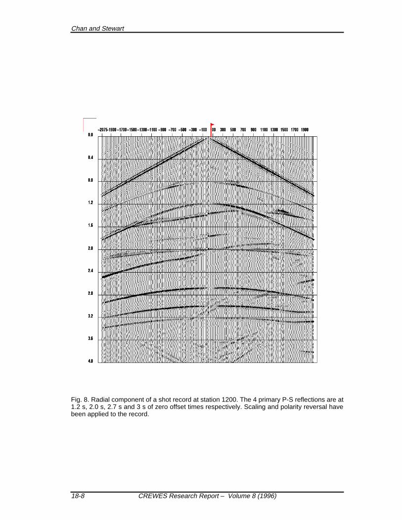
Fig. 8. Radial component of a shot record at station 1200. The 4 primary P-S reflections are at1.2 s, 2.0 s, 2.7 s and 3 s of zero offset times respectively. Scaling and polarity reversal havebeen applied to the record.



Fig. 9. A P-P CMP gather at station 1200. Note that the event at 1.35 seconds is symmetric withrespect to the offset.

Chan and Stewart


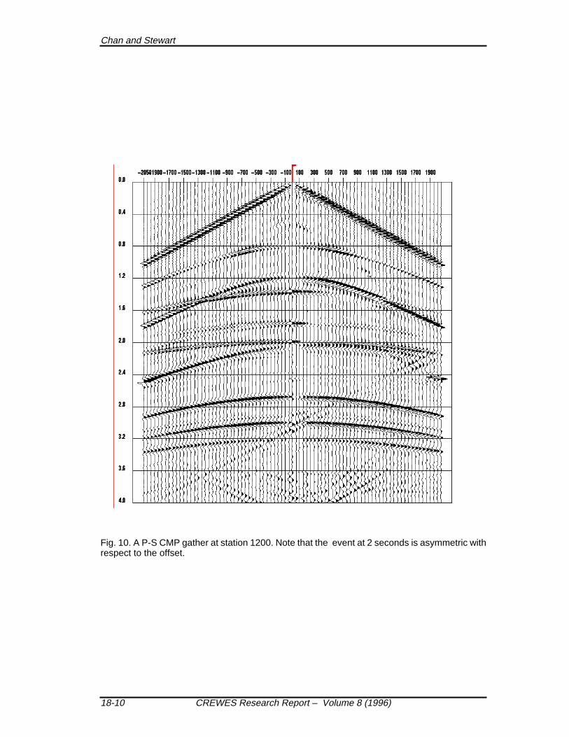
Fig. 10. A P-S CMP gather at station 1200. Note that the event at 2 seconds is asymmetric withrespect to the offset.



Fig. 11. P-P DMO stack.

Chan and Stewart


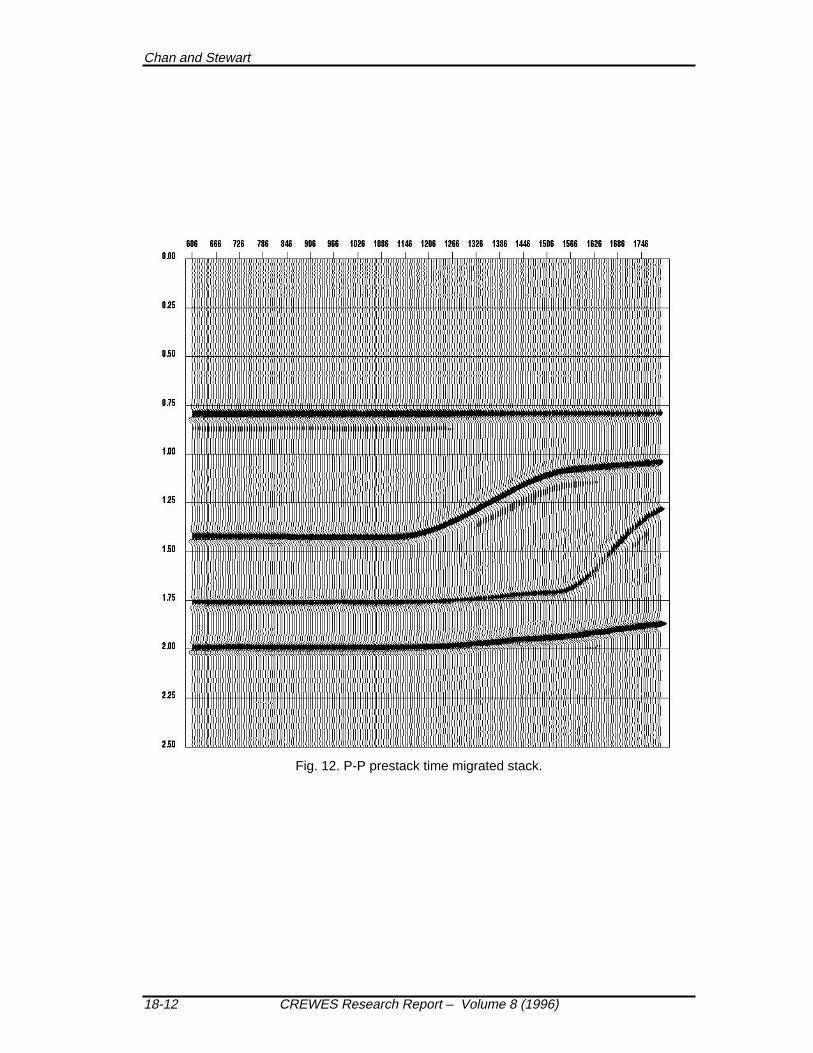
Fig. 12. P-P prestack time migrated stack.



Fig. 13. Asymptotic common conversion point (ACCP) stack of P-S data with Vp/Vs=2.0.

Chan and Stewart


Fig. 14. Pseudo P-P DMO stack. A constant Vp/Vs = 1.8. is used for transformation. Note thatthe times of the events do not match with the true P-P DMO stack in Figure 9.



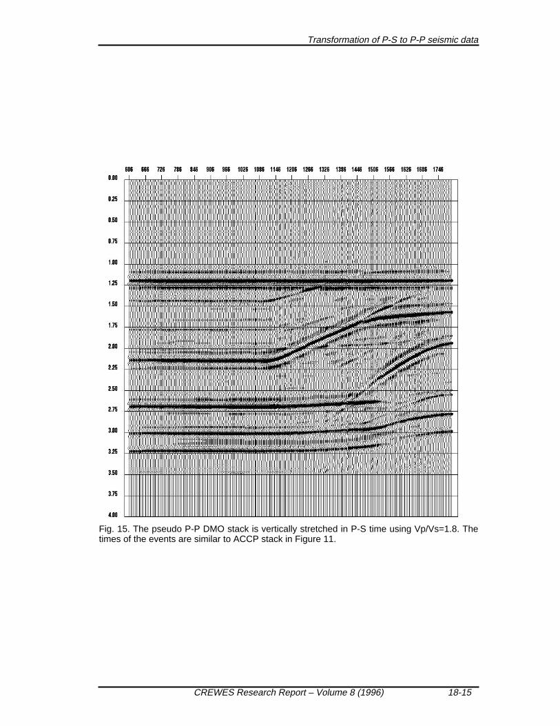
Fig. 15. The pseudo P-P DMO stack is vertically stretched in P-S time using Vp/Vs=1.8. Thetimes of the events are similar to ACCP stack in Figure 11.

Chan and Stewart


Fig. 16. A selected subset of pseudo P-P DMO stack in P-S time for correlation reference. Thisis used, together with the true P-P stack to estimate space-time variant Vp/Vs ratios.



Fig. 17. The corresponding true P-P stack stretched in P-S time using the first estimated Vp/Vsratios from the result of simulated annealing. The times of the events closely match those inFigure 16.

Chan and Stewart


Fig. 18. The pseudo P-P pseudo shot gather at station 1200, using estimated Vp/Vs ratios.



Fig. 19. Same as Figure 18, but with smaller offset range.

Chan and Stewart


Fig. 20. The pseudo P-P CMP gather at station 1200. The reflection from the second layer be-comes symmetric.



Fig. 21. Pseudo P-P DMO stack using the estimated Vp/Vs ratios from the result of simulatedannealing. The times of the events match well with the true P-P DMO stack, except a slight mis-match of the layer occurs at station around 1606.

Chan and Stewart


Fig. 22. The Pseudo P-P DMO stack of Figure 15 in P-S time. It is vertically stretched with theestimated Vp/Vs ratios. This stack also represents P-S DMO stack.



Fig. 23. The pseudo P-P prestack time migrated stack. The events closely match with those inFigure 12, the true P-P time migrated stack.

Chan and Stewart


Fig. 24. The pseudo P-P receiver gather at station 1194. The ASMO is applied in receiver do-main. Note that the valid offset of the events is less than the original input.



Fig. 25. The pseudo P-P CMP gather. The ASMO is applied in receiver domain.It

Chan and Stewart


Fig. 26. The pseudo P-P DMO stack with the transformation applied in receiver domain.Fig. 9.A P-P CMP gather at station 1200. It is noted that the dipping event at 1.35 seconds is sym-metric with respect to the offset.

transformation of p-s to p-p seismic data of p-s to p-p seismic data crewes research report –...

Documents