Transformer Model

Timothy VismorJanuary 23, 2015

Abstract

This document describes a transformer model that is useful for the analysis oflarge scale electric power systems. It defines a balanced transformer representationprimarily intended for use with analytical techniques that are based on the complexnodal admittance matrix. Particular attention is paid to the integration with ”fastdecoupled load flow” (FDLF) algorithms.

Copyright © 1990-2015 Timothy Vismor

CONTENTS LIST OF TABLES

Contents1 Transformer Equivalent Circuit 4

2 Transformer Parameters 52.1 Leakage Impedance . . . . . . . . . . . . . . . . . . . . . . . . . . . . . . 62.2 Voltage Transformation . . . . . . . . . . . . . . . . . . . . . . . . . . . . 7

2.2.1 Transformation Ratio . . . . . . . . . . . . . . . . . . . . . . . . . 72.2.2 Phase Shift . . . . . . . . . . . . . . . . . . . . . . . . . . . . . . . 8

2.3 Voltage Regulation . . . . . . . . . . . . . . . . . . . . . . . . . . . . . . 8

3 Transformer Admittance Model 9

4 Computing Admittances 114.1 Self Admittances . . . . . . . . . . . . . . . . . . . . . . . . . . . . . . . . 11

4.1.1 Primary Admittance . . . . . . . . . . . . . . . . . . . . . . . . . 114.1.2 Secondary Admittance . . . . . . . . . . . . . . . . . . . . . . . . 12

4.2 Transfer Admittances . . . . . . . . . . . . . . . . . . . . . . . . . . . . . 124.2.1 Primary to Secondary . . . . . . . . . . . . . . . . . . . . . . . . . 124.2.2 Secondary to Primary . . . . . . . . . . . . . . . . . . . . . . . . . 134.2.3 Observations on Computational Sequence . . . . . . . . . . . . . 13

5 TCUL Devices 145.1 Computing Tap Adjustments . . . . . . . . . . . . . . . . . . . . . . . . . 145.2 Error Feedback Formulation . . . . . . . . . . . . . . . . . . . . . . . . . 155.3 Controlled Bus Sensitivity . . . . . . . . . . . . . . . . . . . . . . . . . . 165.4 Physical Constraints on Tap Settings . . . . . . . . . . . . . . . . . . . . 17

6 Transformers in the Nodal Admittance Matrix 17

7 The Nodal Admittance Matrix during TCUL 18

8 Integrating TCUL into FDLF 19

List of Tables1 Per Unit to Ohm Conversion Constants . . . . . . . . . . . . . . . . . . . 72 Transformer Phase Shifts . . . . . . . . . . . . . . . . . . . . . . . . . . . 83 Common Transformer Tap Parameters . . . . . . . . . . . . . . . . . . . 94 Ybus Maintenance Costs . . . . . . . . . . . . . . . . . . . . . . . . . . . 20

2

LIST OF FIGURES LIST OF FIGURES

List of Figures1 Transformer Equivalent Circuit Diagram . . . . . . . . . . . . . . . . . . 5

3

1 TRANSFORMER EQUIVALENT CIRCUIT

1 Transformer Equivalent Circuit

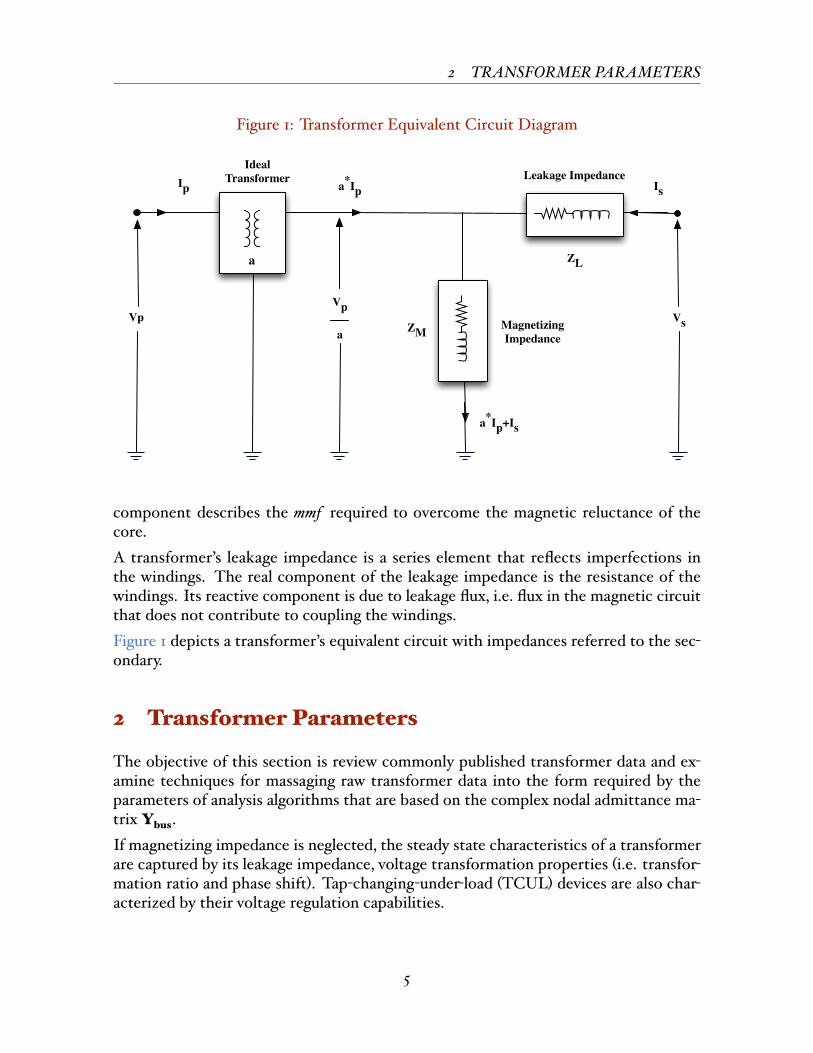
The equivalent circuit of a two winding transformer consists of an ideal transformer,a leakage impedance ZL, and a magnetizing impedance ZM. An ideal transformer is alossless entity categorized by a complex voltage ratio a, i.e.

𝐚 =𝐕𝐩

𝐕𝐬(1)

where

Vp is the transformer’s primary voltage.Vs is the transformer’s secondary voltage.

Since the ideal transformer has no losses, it must be true that

𝐒𝐩 = 𝐒𝐬 (2)

or

𝐕𝐩𝐈⋆𝐩 = 𝐕𝐬𝐈⋆

𝐬 (3)

Solving for the secondary current

𝐈⋆𝐬 = (

𝐕𝐩

𝐕𝐬 ) 𝐈⋆𝐩 (4)

𝐈𝐬 = (𝐕𝐩

𝐕𝐬 )⋆

𝐈𝐩 (5)

Substituting Equation 1 reveals the relationship between the primary and secondarycurrent of an ideal transformer

𝐈𝐬 = 𝐚⋆𝐈𝐩 (6)

where

Ip is current into the transformer’s primary.Is is current out of the transformer’s secondary.a is the transformer’s voltage transformation ratio.

A transformer’s magnetizing impedance is a shunt element associated with its excita-tion current, i.e. the “no load” current in the primary windings. The real componentof the magnetizing impedance reflects the core losses of the transformer. Its reactive

4

2 TRANSFORMER PARAMETERS

Figure 1: Transformer Equivalent Circuit Diagram

a*IpIp Is

Ideal Transformer

Magnetizing Impedance

Leakage Impedance

ZM

ZL

Vp Vs

Vp

a

a*Ip+Is

a

component describes the mmf required to overcome the magnetic reluctance of thecore.A transformer’s leakage impedance is a series element that reflects imperfections inthe windings. The real component of the leakage impedance is the resistance of thewindings. Its reactive component is due to leakage flux, i.e. flux in the magnetic circuitthat does not contribute to coupling the windings.Figure 1 depicts a transformer’s equivalent circuit with impedances referred to the sec-ondary.

2 Transformer Parameters

The objective of this section is review commonly published transformer data and ex-amine techniques for massaging raw transformer data into the form required by theparameters of analysis algorithms that are based on the complex nodal admittance ma-trix Ybus.If magnetizing impedance is neglected, the steady state characteristics of a transformerare captured by its leakage impedance, voltage transformation properties (i.e. transfor-mation ratio and phase shift). Tap-changing-under-load (TCUL) devices are also char-acterized by their voltage regulation capabilities.

5

2.1 Leakage Impedance 2 TRANSFORMER PARAMETERS

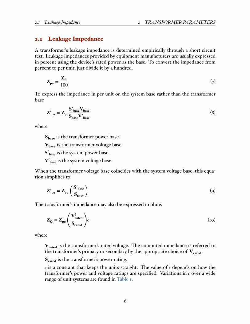
2.1 Leakage Impedance

A transformer’s leakage impedance is determined empirically through a short-circuittest. Leakage impedances provided by equipment manufacturers are usually expressedin percent using the device’s rated power as the base. To convert the impedance frompercent to per unit, just divide it by a hundred.

𝐙𝐩𝐮 = 𝐙%100 (7)

To express the impedance in per unit on the system base rather than the transformerbase

𝐙′𝐩𝐮 = 𝐙𝐩𝐮𝐒′𝐛𝐚𝐬𝐞𝐕𝐛𝐚𝐬𝐞𝐒𝐛𝐚𝐬𝐞𝐕′𝐛𝐚𝐬𝐞

(8)

where

Sbase is the transformer power base.Vbase is the transformer voltage base.𝐒′𝐛𝐚𝐬𝐞 is the system power base.𝐕′𝐛𝐚𝐬𝐞 is the system voltage base.

When the transformer voltage base coincides with the system voltage base, this equa-tion simplifies to

𝐙′𝐩𝐮 = 𝐙𝐩𝐮 (𝐒′𝐛𝐚𝐬𝐞𝐒𝐛𝐚𝐬𝐞 ) (9)

The transformer’s impedance may also be expressed in ohms

𝐙𝛀 = 𝐙𝐩𝐮 (𝐕𝟐

𝐫𝐚𝐭𝐞𝐝𝐒𝐫𝐚𝐭𝐞𝐝 )

𝑐 (10)

where

Vrated is the transformer’s rated voltage. The computed impedance is referred tothe transformer’s primary or secondary by the appropriate choice of Vrated.Srated is the transformer’s power rating.c is a constant that keeps the units straight. The value of c depends on how thetransformer’s power and voltage ratings are specified. Variations in c over a widerange of unit systems are found in Table 1.

6

2.2 Voltage Transformation 2 TRANSFORMER PARAMETERS

Table 1: Per Unit to Ohm Conversion Constants

Voltage Unit Power Unit Constant

Vln VA1𝜑 1Vln VA3𝜑 3Vln kVA1𝜑 1/1,000Vln kVA3𝜑 3/1,000Vll VA1𝜑 1/3Vll VA3𝜑 1Vll kVA1𝜑 1/3,000Vll kVA3𝜑 1/1,000kVln kVA1𝜑 1,000kVln kVA3𝜑 3,000kVln MVA1𝜑 1kVln MVA3𝜑 3kVll kVA1𝜑 1,000/3kVll kVA3𝜑 1,000kVll MVA1𝜑 1/3kVll MVA3𝜑 1

2.2 Voltage Transformation

A transformer’s voltage ratio is expressed in polar form as ae𝑗𝛿, where a is the magnitudeof the transformation and 𝛿 is its phase shift.

2.2.1 Transformation Ratio

Each transformer is categorized by a nominal operating point, i.e. its nameplate primaryand secondary voltage. The nominal magnitude of the voltage ratio is determined byexamining the real part of Equation 1 at nominal operating conditions.

𝑎𝑛𝑜𝑚 =𝑉𝑝

𝑉𝑠(11)

where

Vp is the nominal primary voltage.Vs is the nominal secondary voltage.

When voltages are expressed in per unit, the nominal value of a is always one.

7

2.3 Voltage Regulation 2 TRANSFORMER PARAMETERS

2.2.2 Phase Shift

In the general case, an arbitrary angular shift 𝛿 may be introduced by a multiphase trans-former bank. However, omitting phase shifters (angle regulating transformers) fromthe system model, reduces the angle shifts across balanced transformer configurationsto effects introduced by the connections of the windings. Table 2 describes the phaseshift associated with common transformer connections.

Table 2: Transformer Phase Shifts

WindingPrimary Secondary Phase Shift

Wye Wye 0∘

Wye Delta −30∘

Delta Wye 30∘

Delta Delta 0∘

When phase shifters are ignored, the user does not have to specify 𝛿 explicitly. It maybe inferred from Table 2.

2.3 Voltage Regulation

Most power transformers permit you to tap into the windings at a variety of differentpositions. Some transformers are configured with voltage sensors and motors whichpermit them to change tap settings automatically in response to voltage variations onthe power system. These transformers are referred to as tap-changing-under-Ioad (TCUL)devices. A TCUL device that controls voltage but does not transform large amountsof power is referred to as a regulating transformer. Regulating transformers that con-trol voltage magnitude on distribution systems are usually called voltage regulators orsimply regulators.TCUL devices that regulate voltage magnitudes are categorized by a tap range and a tapincrement. The tap range defines the limits of the device’s regulating ability. The tapincrement defines the resolution of the device. The tap changing mechanism of manytransformers is categorized by a regulation range and a step count, e.g. ±10 percent, 32steps. The tap increment is computed from this data as follows.

𝑇𝑖𝑛𝑐 = 𝑇𝑚𝑎𝑥 − 𝑇𝑚𝑖𝑛𝑛𝑠𝑡𝑒𝑝𝑠

(12)

where

8

3 TRANSFORMER ADMITTANCE MODEL

Tinc is the transformer’s tap increment.Tmax is maximum increase in voltage provided by the transformer (sometimes calledboost). If the transformer can not boost the voltage, Tmax is zero.Tmin is maximum decrease in voltage provided by the transformer (sometimes calledbuck). If the transformer can not decrease the voltage, Tmin is zero.nsteps is the number of tap steps.

Table 3 catalogs the tap range and increment of common load tap-changers.

Table 3: Common Transformer Tap Parameters

Regulation Range nsteps Tmax Tmin Tinc

±10% 32 10.0 -10.0 0.62500±10% 16 10.0 -10.0 1.25000±10% 8 10.0 -10.0 2.50000+10% 32 10.0 0.0 0.31250+10% 16 10.0 0.0 0.62500+10% 8 10.0 0.0 1.25000±7.5% 32 7.5 -7.5 0.46875±7.5% 16 7.5 -7.5 0.93750±7.5% 8 7.5 -7.5 1.87500+7.5% 32 7.5 0.0 0.23437+7.5% 16 7.5 0.0 0.46875+7.5% 8 7.5 0.0 0.93750±5% 32 5.0 -5.0 0.31250±5% 16 5.0 -5.0 0.62500±5% 8 5.0 -5.0 1.25000+5% 32 10.0 0.0 0.15625+5% 16 10.0 0.0 0.31250+5% 8 10.0 0.0 0.62500

3 Transformer Admittance Model

For analysis purposes, each transformer is described by the admittances of a generaltwo-port network. When the current equations of Figure 1 are written as follows, thetransformer admittances correspond to the coefficient matrix.

𝐈𝐩 = 𝐘𝐩𝐩𝐕𝐩 + 𝐘𝐩𝐬𝐕𝐬 (13)𝐈𝐬 = 𝐘𝐬𝐩𝐕𝐩 + 𝐘𝐬𝐬𝐕𝐬 (14)

where

9

3 TRANSFORMER ADMITTANCE MODEL

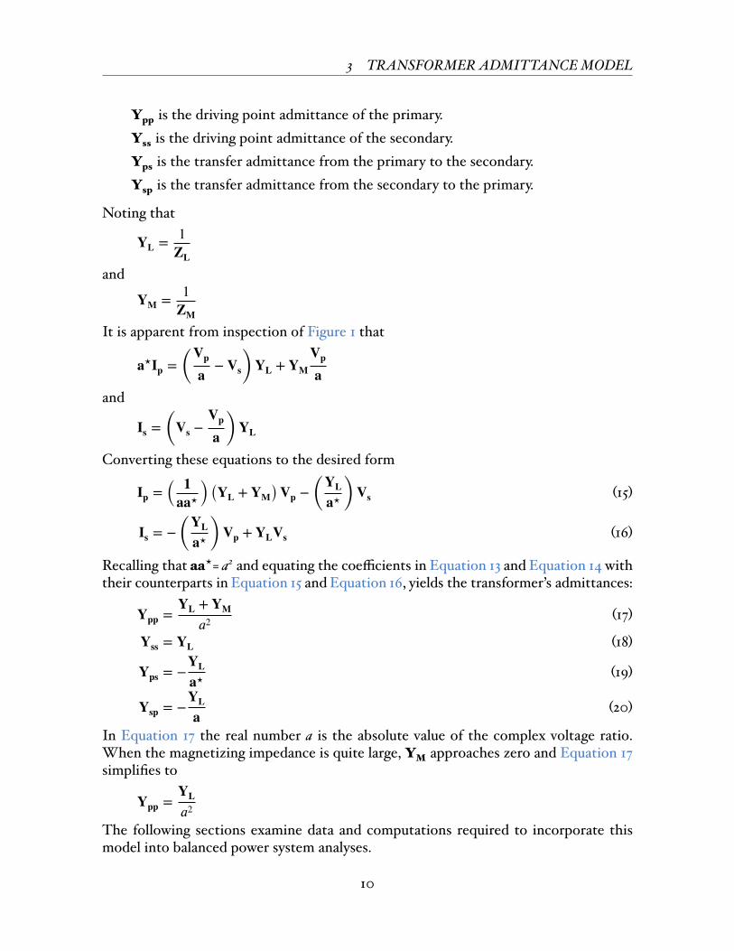
Ypp is the driving point admittance of the primary.Yss is the driving point admittance of the secondary.Yps is the transfer admittance from the primary to the secondary.Ysp is the transfer admittance from the secondary to the primary.

Noting that

𝐘𝐋 = 1𝐙𝐋

and

𝐘𝐌 = 1𝐙𝐌

It is apparent from inspection of Figure 1 that

𝐚⋆𝐈𝐩 = (𝐕𝐩

𝐚 − 𝐕𝐬) 𝐘𝐋 + 𝐘𝐌𝐕𝐩

𝐚and

𝐈𝐬 = (𝐕𝐬 −𝐕𝐩

𝐚 ) 𝐘𝐋

Converting these equations to the desired form

𝐈𝐩 = (𝟏

𝐚𝐚⋆ ) (𝐘𝐋 + 𝐘𝐌) 𝐕𝐩 − (𝐘𝐋𝐚⋆ ) 𝐕𝐬 (15)

𝐈𝐬 = − (𝐘𝐋𝐚⋆ ) 𝐕𝐩 + 𝐘𝐋𝐕𝐬 (16)

Recalling that aa⋆= a2 and equating the coefficients in Equation 13 and Equation 14 withtheir counterparts in Equation 15 and Equation 16, yields the transformer’s admittances:

𝐘𝐩𝐩 = 𝐘𝐋 + 𝐘𝐌𝑎2 (17)

𝐘𝐬𝐬 = 𝐘𝐋 (18)

𝐘𝐩𝐬 = −𝐘𝐋𝐚⋆ (19)

𝐘𝐬𝐩 = −𝐘𝐋𝐚 (20)

In Equation 17 the real number a is the absolute value of the complex voltage ratio.When the magnetizing impedance is quite large, YM approaches zero and Equation 17simplifies to

𝐘𝐩𝐩 = 𝐘𝐋𝑎2

The following sections examine data and computations required to incorporate thismodel into balanced power system analyses.

10

4 COMPUTING ADMITTANCES

4 Computing Admittances

This section examines Equation 17 through Equation 20 with an eye for streamliningtheir computation. The resulting computational sequence explicitly decomposes thecomplex equations into real operations.A transformer’s leakage admittance YL is derived from the leakage impedance ZL inthe usual manner. Expressing the leakage impedance in rectangular form

𝐙𝐋 = 𝑟𝐿 + 𝑗𝑥𝐿 (21)

then

𝐘𝐋 = 1𝐙𝐋

= 1𝑟𝐿 + 𝑗𝑥𝐿

= 𝑔𝐿 + 𝑗𝑏𝐿 (22)

where

𝑔𝐿 = 𝑟𝐿

𝑟2𝐿 + 𝑥2

𝐿(23)

𝑏𝐿 = − 𝑥𝐿

𝑟2𝐿 + 𝑥2

𝐿(24)

For the sake of convenience, define the tap ratio as

𝐭 = 1𝐚 = 𝑡𝑒𝑗−𝛿 (25)

4.1 Self Admittances

In the context of modeling and analysis of electrical networks, the self admittances ofa transformer can be thought of as the device’s impact on the diagonal elements of ofthe nodal admittance matrix Ybus.

4.1.1 Primary Admittance

Considering the self admittance of the transformer’s primary, Equation 17 states

𝐘𝐩𝐩 = 𝐘𝐋 + 𝐘𝐌𝑎2 (26)

Expressing the complex equation in rectangular form and making the substitution de-fined in Equation 25

𝐘𝐩𝐩 = 𝑡2(𝑔𝐿 + 𝑔𝑀 ) + 𝑗𝑡2(𝑏𝐿 + 𝑏𝑀 ) (27)

When the magnetizing admittance is ignored, Equation 27 reduces to

𝐘𝐩𝐩 = 𝑡2𝑔𝐿 + 𝑗𝑡2𝑏𝐿 (28)

11

4.2 Transfer Admittances 4 COMPUTING ADMITTANCES

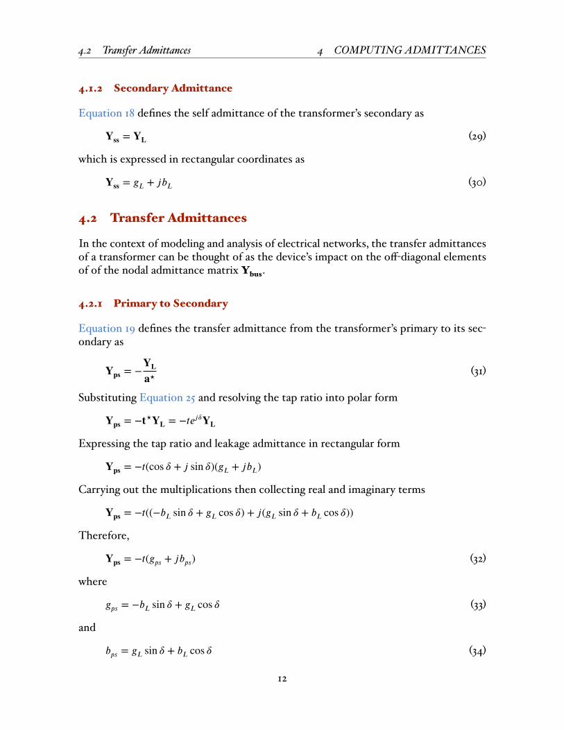
4.1.2 Secondary Admittance

Equation 18 defines the self admittance of the transformer’s secondary as

𝐘𝐬𝐬 = 𝐘𝐋 (29)

which is expressed in rectangular coordinates as

𝐘𝐬𝐬 = 𝑔𝐿 + 𝑗𝑏𝐿 (30)

4.2 Transfer Admittances

In the context of modeling and analysis of electrical networks, the transfer admittancesof a transformer can be thought of as the device’s impact on the off-diagonal elementsof of the nodal admittance matrix Ybus.

4.2.1 Primary to Secondary

Equation 19 defines the transfer admittance from the transformer’s primary to its sec-ondary as

𝐘𝐩𝐬 = −𝐘𝐋𝐚⋆ (31)

Substituting Equation 25 and resolving the tap ratio into polar form

𝐘𝐩𝐬 = −𝐭⋆𝐘𝐋 = −𝑡𝑒𝑗𝛿𝐘𝐋

Expressing the tap ratio and leakage admittance in rectangular form

𝐘𝐩𝐬 = −𝑡(cos 𝛿 + 𝑗 sin 𝛿)(𝑔𝐿 + 𝑗𝑏𝐿)

Carrying out the multiplications then collecting real and imaginary terms

𝐘𝐩𝐬 = −𝑡((−𝑏𝐿 sin 𝛿 + 𝑔𝐿 cos 𝛿) + 𝑗(𝑔𝐿 sin 𝛿 + 𝑏𝐿 cos 𝛿))

Therefore,

𝐘𝐩𝐬 = −𝑡(𝑔𝑝𝑠 + 𝑗𝑏𝑝𝑠) (32)

where

𝑔𝑝𝑠 = −𝑏𝐿 sin 𝛿 + 𝑔𝐿 cos 𝛿 (33)

and

𝑏𝑝𝑠 = 𝑔𝐿 sin 𝛿 + 𝑏𝐿 cos 𝛿 (34)

12

4.2 Transfer Admittances 4 COMPUTING ADMITTANCES

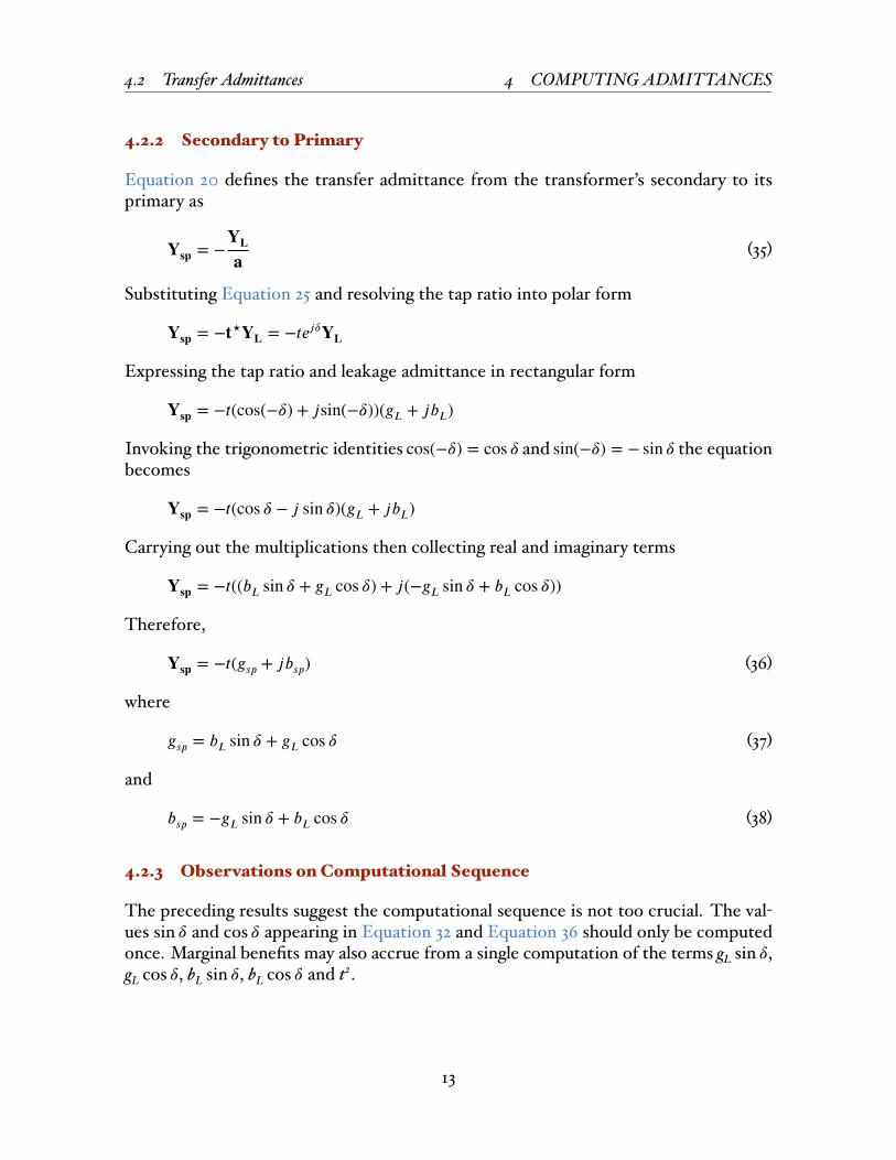
4.2.2 Secondary to Primary

Equation 20 defines the transfer admittance from the transformer’s secondary to itsprimary as

𝐘𝐬𝐩 = −𝐘𝐋𝐚 (35)

Substituting Equation 25 and resolving the tap ratio into polar form

𝐘𝐬𝐩 = −𝐭⋆𝐘𝐋 = −𝑡𝑒𝑗𝛿𝐘𝐋

Expressing the tap ratio and leakage admittance in rectangular form

𝐘𝐬𝐩 = −𝑡(cos(−𝛿) + 𝑗sin(−𝛿))(𝑔𝐿 + 𝑗𝑏𝐿)

Invoking the trigonometric identities cos(−𝛿) = cos 𝛿 and sin(−𝛿) = − sin 𝛿 the equationbecomes

𝐘𝐬𝐩 = −𝑡(cos 𝛿 − 𝑗 sin 𝛿)(𝑔𝐿 + 𝑗𝑏𝐿)

Carrying out the multiplications then collecting real and imaginary terms

𝐘𝐬𝐩 = −𝑡((𝑏𝐿 sin 𝛿 + 𝑔𝐿 cos 𝛿) + 𝑗(−𝑔𝐿 sin 𝛿 + 𝑏𝐿 cos 𝛿))

Therefore,

𝐘𝐬𝐩 = −𝑡(𝑔𝑠𝑝 + 𝑗𝑏𝑠𝑝) (36)

where

𝑔𝑠𝑝 = 𝑏𝐿 sin 𝛿 + 𝑔𝐿 cos 𝛿 (37)

and

𝑏𝑠𝑝 = −𝑔𝐿 sin 𝛿 + 𝑏𝐿 cos 𝛿 (38)

4.2.3 Observations on Computational Sequence

The preceding results suggest the computational sequence is not too crucial. The val-ues sin 𝛿 and cos 𝛿 appearing in Equation 32 and Equation 36 should only be computedonce. Marginal benefits may also accrue from a single computation of the terms gL sin 𝛿,gL cos 𝛿, bL sin 𝛿, bL cos 𝛿 and t2.

13

5 TCUL DEVICES

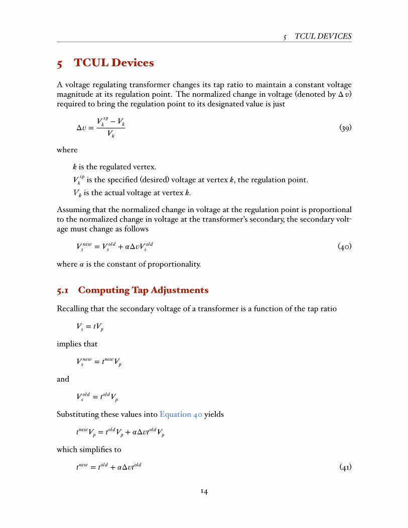
5 TCUL Devices

A voltage regulating transformer changes its tap ratio to maintain a constant voltagemagnitude at its regulation point. The normalized change in voltage (denoted by Δ v)required to bring the regulation point to its designated value is just

Δ𝑣 =𝑉 𝑠𝑝

𝑘 − 𝑉𝑘𝑉𝑘

(39)

where

k is the regulated vertex.𝑉 𝑠𝑝

𝑘 is the specified (desired) voltage at vertex k, the regulation point.Vk is the actual voltage at vertex k.

Assuming that the normalized change in voltage at the regulation point is proportionalto the normalized change in voltage at the transformer’s secondary, the secondary volt-age must change as follows

𝑉 𝑛𝑒𝑤𝑠 = 𝑉 𝑜𝑙𝑑

𝑠 + 𝛼Δ𝑣𝑉 𝑜𝑙𝑑𝑠 (40)

where 𝛼 is the constant of proportionality.

5.1 Computing Tap Adjustments

Recalling that the secondary voltage of a transformer is a function of the tap ratio

𝑉𝑠 = 𝑡𝑉𝑝

implies that

𝑉 𝑛𝑒𝑤𝑠 = 𝑡𝑛𝑒𝑤𝑉𝑝

and

𝑉 𝑜𝑙𝑑𝑠 = 𝑡𝑜𝑙𝑑𝑉𝑝

Substituting these values into Equation 40 yields

𝑡𝑛𝑒𝑤𝑉𝑝 = 𝑡𝑜𝑙𝑑𝑉𝑝 + 𝛼Δ𝑣𝑡𝑜𝑙𝑑𝑉𝑝

which simplifies to

𝑡𝑛𝑒𝑤 = 𝑡𝑜𝑙𝑑 + 𝛼Δ𝑣𝑡𝑜𝑙𝑑 (41)

14

5.2 Error Feedback Formulation 5 TCUL DEVICES

To obtain a computational formula, substitute Equation 39

𝑡𝑛𝑒𝑤 = 𝑡𝑜𝑙𝑑 + 𝛼𝑡𝑜𝑙𝑑 𝑉 𝑠𝑝𝑘 − 𝑉𝑘

𝑉𝑘

and simplify as follows

𝑡𝑛𝑒𝑤 = 𝑡𝑜𝑙𝑑 + 𝛼𝑡𝑜𝑙𝑑(𝑉 𝑠𝑝

𝑘𝑉𝑘

− 1) = 𝑡𝑜𝑙𝑑 + 𝛼𝑡𝑜𝑙𝑑 𝑉 𝑠𝑝𝑘

𝑉𝑘− 𝛼𝑡𝑜𝑙𝑑

or

𝑡𝑛𝑒𝑤 = 𝑡𝑜𝑙𝑑(1 − 𝛼 + 𝛼𝑉 𝑠𝑝

𝑘𝑉𝑘

) (42)

Normally, 𝛼 is assumed to be one and Equation 42 reduces to

𝑡𝑛𝑒𝑤 = 𝑡𝑜𝑙𝑑(

𝑉 𝑠𝑝𝑘

𝑉𝑘 ) (43)

Computation of 𝛼, the sensitivity of the regulated voltage to transformer tap changes,is discussed in Section 5.3.

5.2 Error Feedback Formulation

Stott and Alsac (1974) and Chan and Brandwajn (1986) describe transformer tap adjust-ments as an error feedback formula

𝑎𝑛𝑒𝑤 − 𝑎𝑜𝑙𝑑 = 𝛼 (𝑉 𝑠𝑝

𝑘𝑉𝑘 ) (44)

where all quantities are expressed in per unit. The per unit voltage transformation ratioapu is computed as follows

𝑎𝑝𝑢 =𝑉 𝑝𝑢

𝑝

𝑉 𝑝𝑢𝑠

=𝑉𝑝

𝑉 𝑛𝑜𝑚𝑝𝑉𝑠

𝑉 𝑛𝑜𝑚𝑠

which simplifies to

𝑎𝑝𝑢 =𝑉 𝑛𝑜𝑚

𝑠𝑉𝑝

𝑉 𝑛𝑜𝑚𝑝

𝑉𝑠= (

𝑉𝑝

𝑉𝑠 ) (𝑉 𝑛𝑜𝑚

𝑠𝑉 𝑛𝑜𝑚

𝑝 ) = 𝑎𝑎𝑛𝑜𝑚

where anom is the nominal voltage transformation ratio. Therefore, Equation 44 is equiv-alent to

𝑎𝑛𝑒𝑤

𝑎𝑛𝑜𝑚 − 𝑎𝑜𝑙𝑑

𝑎𝑛𝑜𝑚 = 𝛼𝑉𝑘 − 𝑉 𝑠𝑝

𝑘

𝑉 𝑏𝑎𝑠𝑒𝑘

15

5.3 Controlled Bus Sensitivity 5 TCUL DEVICES

or

𝑎𝑛𝑒𝑤 − 𝑎𝑜𝑙𝑑 = 𝑎𝑛𝑜𝑚𝛼𝑉𝑘 − 𝑉 𝑠𝑝

𝑘

𝑉 𝑏𝑎𝑠𝑒𝑘

in physical quantities. Solving for the updated transformation ratio yields

𝑎𝑛𝑒𝑤 = 𝑎𝑜𝑙𝑑 + 𝑎𝑛𝑜𝑚𝛼𝑉𝑘 − 𝑉 𝑠𝑝

𝑘

𝑉 𝑏𝑎𝑠𝑒𝑘

(45)

Computation of 𝛼, the sensitivity of the regulated voltage to changes in transformationratio, is discussed in Section 5.3.

5.3 Controlled Bus Sensitivity

The proportionality constant 𝛼 (referenced in Equation 45 and Equation 42) representsthe sensitivity of the controlled voltage to tap changes at the regulating transformer.It commonly assumed that 𝛼 is one (the controlled voltage is perfectly sensitive to tapchanges). An alternate assumption is that

𝛼 = M𝑇𝑘 (B″)−1N (46)

where

M𝑇𝑘 is a row vector with 1 in the kth position.

N is a column vector with -bpst in position p and bpst in position s.

Carrying out these matrix operations yields

𝛼 = −𝑏𝑝𝑠𝑡𝑏′′ −1𝑘𝑝 + 𝑏𝑝𝑠𝑡𝑏′′ −1

𝑘𝑠 (47)

where

bij is an element from the nodal susceptance matrix Bbus.

𝑏′′ −1𝑖𝑗 is an element from the inverse of 𝐵″ as defined by Stott and Alsac (1974).

t is magnitude of the transformer’s tap ratio.

Chan and Brandwajn (1986) suggest that sensitivities computed from Equation 47 areuseful for coordinating adjustments to a bus that is controlled by several transformers.

16

5.4 Physical Constraints on Tap Settings6 TRANSFORMERS IN THE NODAL ADMITTANCE MATRIX

5.4 Physical Constraints on Tap Settings

The preceding sections treat a transformer’s tap setting as a continuous quantity. How-ever, tap settings are discrete. There are three ways to handle discrete taps:

• Modify equations Equation 42 and Equation 45 so that the tap setting is computeddiscretely.

• Compute tap settings from Equation 42 or Equation 45. Round the tap setting tothe nearest discrete value each time the tap changes.

• Compute tap settings from Equation 42 or Equation 45. Round the tap settingsafter the load flow has converged. Fix the transformer taps. Continue until thesolution converges with the discrete fixed tap transformers.

As was discussed in Section 2.3, the tap changing mechanism is limited in its regulat-ing abilities. Each TCUL device is subject to tap limits, i.e. maximum and minimumphysically realizable tap settings. The implementation of Equation 42, Equation 43, orEquation 45 should reflect this fact. For example, Equation 43 should be implementedas

𝑡𝑛𝑒𝑤 =⎧⎪⎨⎪⎩

𝑡𝑚𝑖𝑛 if 𝑡𝑛𝑒𝑤 < 𝑡𝑚𝑖𝑛

𝑡𝑜𝑙𝑑(

𝑉 𝑠𝑝𝑘

𝑉𝑘 ) if 𝑡𝑚𝑖𝑛 ≤ 𝑡𝑛𝑒𝑤 ≤ 𝑡𝑚𝑎𝑥

𝑡𝑚𝑎𝑥 if 𝑡𝑛𝑒𝑤 > 𝑡𝑚𝑎𝑥

(48)

6 Transformers in the Nodal Admittance Matrix

The complex nodal admittance matrix is referred to as Ybus. In the current formulation,the admittances of Ybus are stored in rectangular form. The real part of Ybus (theconductance matrix) is called Gbus. The imaginary part of Ybus (the susceptance matrix)is called Bbus. Ybus is formed according to two simple rules.

1. The diagonal terms of Ybus (i.e. yii) are the driving point admittances of the net-work. They are the algebraic sum of all admittances incident upon vertex i. Thesevalues include both the self admittances of incident edges (with respect to vertexi) and shunts to ground at the vertex itself.

2. The off-diagonal terms of Ybus (i.e. yij where i ≠ j) are the transfer admittancesof the edge connecting vertices i and j.

Assuming that each transformer is modeled as two vertices (representing its primaryand secondary terminals) and a connecting edge in the network graph, the procedurefor incorporating a transformer into the nodal admittance matrix is as follows.

1. Compute the admittance matrix of the transformer (i.e. Ypp, Yss, Yps, and Ysp)at the nominal tap setting. See Section 4 for details.

17

7 THE NODAL ADMITTANCE MATRIX DURING TCUL

2. Include the transformer’s primary admittance Ypp as its contribution to the selfadmittance of the primary vertex p. That is, add Ypp to the corresponding diago-nal element of the nodal admittance matrix ypp.

3. Include the transformer’s secondary admittance Yss as its contribution to the selfadmittance of the secondary vertex s. That is, add Yss to the corresponding diag-onal element of the nodal admittance matrix yss.

4. Use Yps as the transfer admittance of the edge from the primary vertex p to thesecondary vertex s (i.e. set the corresponding off-diagonal element of the nodaladmittance matrix yps to Yps).

5. Use Ysp as the transfer admittance of the edge from the secondary vertex s tothe primary vertex p (i.e. set the corresponding off-diagonal element of the nodaladmittance matrix ysp to Ysp).

Note: Examining Equation 19 and Equation 20, you can see that asymmetries intro-duced into Ybus by a transformer are due to the fact that a⋆ is used to compute Yps anda is used to compute Ysp. When a = a⋆, Ybus is symmetric with respect to transformers.This condition is only true when a is real. In this situation, 𝛿 is zero and there is nophase shift across the transformer.

7 The Nodal Admittance Matrix during TCUL

Tap-changing-under-load (TCUL) has an impact on power flow studies since it changesthe voltage transformation ratio thus changing the impedance of a transformer. Theseimpedance adjustments must be reflected in the nodal admitance matrix Ybus. The fol-lowing discussion examines techniques for updating Ybus when a transformer changestap settings.Assume that the following information is required by any procedure that updates Ybusfollowing a tap change:

• Ybus itself,• YL the transformer’s leakage admittance, and• tnew the transformer’s tap ratio after the tap change.

The transfer admittances (off-diagonal elements of Ybus) can be maintained with thisbase of information. However, maintaining the self admittances is more complicated.There are two strategies for updating the diagonal of Ybus.

• Rebuild the entry from scratch, or• Back out the old transformer admittances, then add in the new values.

The reconstruction strategy is ruled out as computationally inefficient without exten-sive examination. Computational requirements of rebuilding an entry include:

18

8 INTEGRATING TCUL INTO FDLF

• Compute the new admittances of the TCUL device.• Access the incidence list of the primary vertex p.• Look up shunt elements (e.g. impedance loads) at the primary vertex p.• Recompute the self admittances of any transformers adjacent to the TCUL device

(incident upon its primary vertex).The direct update strategy is examined more carefully. Its basic computational com-plexity stems from backing the old value of the transformer’s primary admittance Yppout of ypp (the self admittance of vertex p). There are two ways to proceed:

1. Remember Ypp so that it can be backed out directly, or2. Recompute Ypp, then back it out of ypp. From Equation 27 or Equation 28, it is

seen that the square of told (the magnitude of the original tap ratio) is needed torecompute Ypp.

The Ybus maintenance algorithm based on a direct update approach follows.1. Determine the transformer’s original primary admittance Ypp, subtract it from

the corresponding diagonal term of the nodal admittance matrix ypp.2. Compute the new primary admittance Ypp using Equation 27 or Equation 28, add

it to the corresponding diagonal term of the nodal admittance matrix ypp.3. Compute the new transfer admittance Yps from Equation 32, set the correspond-

ing off-diagonal element of the admittance matrix yps to this value.4. Compute the new transfer admittance Ysp using Equation 36, set the correspond-

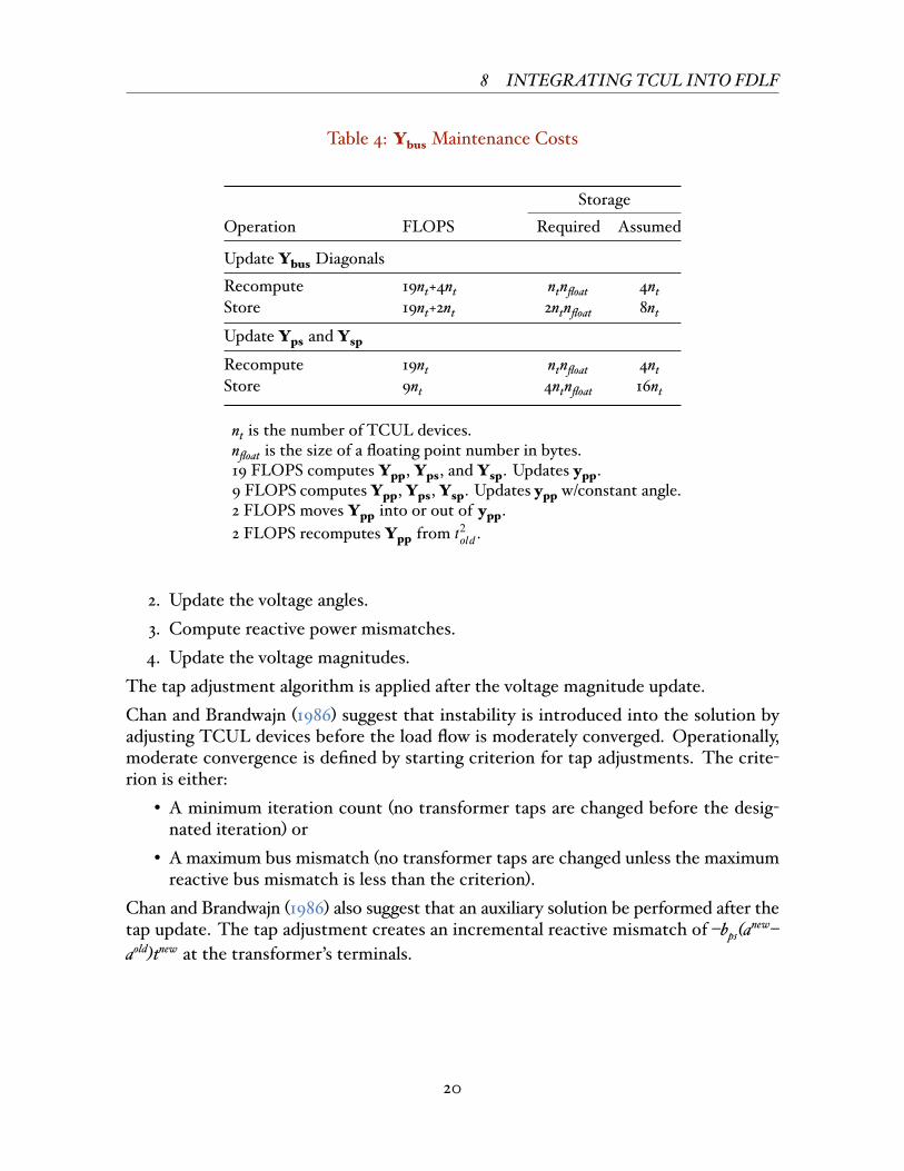
ing off-diagonal element of the admittance matrix ysp to this value.Examining Equation 30, you should observe that the transformer’s secondary admit-tance Yss is not a function of the tap setting. Therefore, it does not have to be updatedwhen the tap changes.When 𝛿 does not change during the load flow (i.e. no phase angle regulators), theterms gL sin 𝛿, gL cos 𝛿, bL sin 𝛿, bL cos 𝛿 in Equation 32 and Equation 36 remain constantthroughout the load flow solution. If these terms are precomputed and stored, a con-siderable reduction in floating point arithmetic results. Obviously, you pay a price instorage. Table 4 summarizes the time and space trade-offs associated with recomputu-taion vs storage of these products when updating the diagonal of Ybus and computingthe transfer admittances Yps and Ysp in the absence of phase angle regulators.

8 Integrating TCUL into FDLF

A fast decoupled load flow (FDLF) iteration consists of four basic steps:1. Compute real power mismatches.

19

8 INTEGRATING TCUL INTO FDLF

Table 4: Ybus Maintenance Costs

StorageOperation FLOPS Required Assumed

Update Ybus DiagonalsRecompute 19nt+4nt ntnfloat 4ntStore 19nt+2nt 2ntnfloat 8nt

Update Yps and Ysp

Recompute 19nt ntnfloat 4ntStore 9nt 4ntnfloat 16nt

nt is the number of TCUL devices.nfloat is the size of a floating point number in bytes.19 FLOPS computes Ypp, Yps, and Ysp. Updates ypp.9 FLOPS computes Ypp, Yps, Ysp. Updates ypp w/constant angle.2 FLOPS moves Ypp into or out of ypp.2 FLOPS recomputes Ypp from 𝑡2

𝑜𝑙𝑑 .

2. Update the voltage angles.3. Compute reactive power mismatches.4. Update the voltage magnitudes.

The tap adjustment algorithm is applied after the voltage magnitude update.Chan and Brandwajn (1986) suggest that instability is introduced into the solution byadjusting TCUL devices before the load flow is moderately converged. Operationally,moderate convergence is defined by starting criterion for tap adjustments. The crite-rion is either:

• A minimum iteration count (no transformer taps are changed before the desig-nated iteration) or

• A maximum bus mismatch (no transformer taps are changed unless the maximumreactive bus mismatch is less than the criterion).

Chan and Brandwajn (1986) also suggest that an auxiliary solution be performed after thetap update. The tap adjustment creates an incremental reactive mismatch of –bps(anew–aold)tnew at the transformer’s terminals.

20

REFERENCES REFERENCES

References

Chan, S. and V. Brandwajn (1986). “Partial matrix refactorization”. In: IEEE Transactionson Power Systems 1.1, pp. 193–200 (cit. on pp. 15, 16, 20).

Stott, B. and O. Alsac (1974). “Fast decoupled load flow”. In: IEEE Transactions on PowerApparatus and Systems 93.3, pp. 859–869 (cit. on pp. 15, 16).

21