3. TRANSFORMERS Although the static transformer is not an energy-conversion device, it is an indispendable component in many energy-conversion systems. As one of the principal reasons for the widespread use of AC systems, it makes possible electric generation at the most economical generator voltage, power transfer at the most economical transmission voltage and power utilization at the most suitable voltage for the particular utilization device. The transformer is also widely used in low-power, low-current electronic and control circuits for performing such function as matching the impedances of source and it's load maximum power transfer, insulating one circuit from another, or isolating direct current while maintaing AC continuity between two circuits.

Essentially, a transformer consist two or more windings interlinked by a mutual magnetic field.

If one of these windings, the primary, is connected to an alternating-voltage source, an alternating flux will be produced whose amplitude will depend on the primary voltage and number of turns. The mutual flux will link the other winding, the secondary, and will induce a voltage in it which value will depend on the number of secondary turns.

Dividing the numbers of primary turns by the number of secondary turns, almost any desired ratio, or ratio of transformation, can be obtained.

In a transformer we can use air core, but the transformer action will be obtained more effectively with a core of iron or other ferromagnetic material, because most of the flux is confined to a definite path linking both windings and having a much higher permeability then that of air. Such a transformer is commonly called an iron-core transformer.

Therefore first we examine the iron losses and the excitation of the magnetic circuit. In a transformer the magnetic materials can be used in well-defined path, and they are used to maximise the coupling between the windings as well as to lower the excitation current required for transformer operation.

ϕ (t) (main flux lines)

leakage fluxϕ l1

ϕ l2N2

secondarywinding

(primary)windingsupplied

N1e1 e2

laminated iron core

Fig. 3.1. Elementary built up of a transformer

2

Ferromagnetic materials are composed of iron and alloys of iron with silicon, cobalt, nickel, aluminium and other metals.

The relation between B and H is both non-linear and multivalued. In general, the characteristics of the material cannot be described analytically. They are commonly presented in graphical form, and are measured using methods prescribed by standards.

The most common curve used to describe a magnetic material is the B-H curve or hysteresis loop (Fig. 3.2.).

Each curve is obtained while cyclically varying the applied magnetizing force between equal poisitive and negative values of fixed magnitude. The arrows shows the path followed by B with increasing and decreasing H, notice that with increasing magnitude of H the curves begin to flatten out as the material tends toward saturation (Fig. 3.3.).

The magnetic materials can be described with DC or normal magnetization curve too.

B

H H

B

Br

Br

Hc

saturation

first magnetizationcurve

coercitive force

remanent orresudial flux

density

magneticmaterial

soft

magneticmaterial

permanent

H [A/m]

B [T]

0,60,70,80,91,0

0,10,20,30,40,5

1,61,71,81,9

1,11,21,31,41,5

2,0

0,60,70,80,91,0

0,10,20,30,40,5

1,61,71,81,9

1,11,21,31,41,5

2,0

300100 400200 500 800600 900700 1000

cold-rolled strip

warm-rolled strip

3.2.. ábra Magnetization curve of transformers core-sheets

3

Fig. 3.2. B-H loops of different magnetic materials

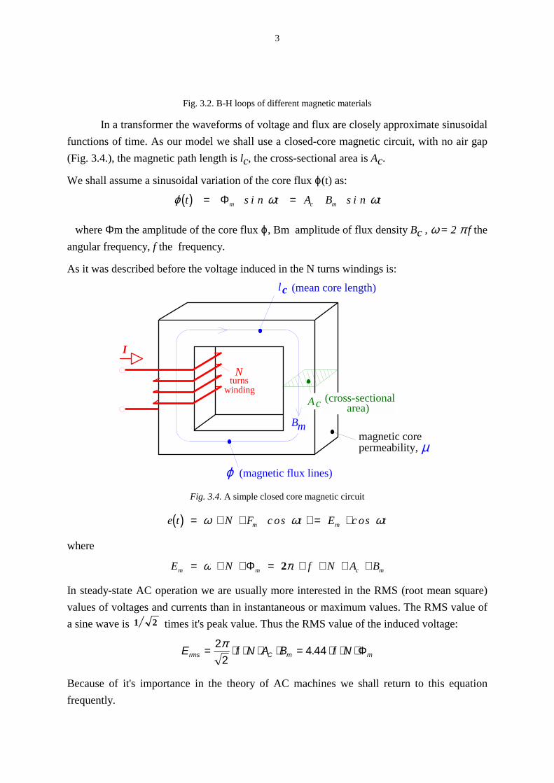
In a transformer the waveforms of voltage and flux are closely approximate sinusoidal functions of time. As our model we shall use a closed-core magnetic circuit, with no air gap (Fig. 3.4.), the magnetic path length is lc, the cross-sectional area is Ac.

We shall assume a sinusoidal variation of the core flux ϕ(t) as:

( )ϕ ω ωt t A B tm c m= =Φ s i n s i n

where Φm the amplitude of the core flux ϕ, Bm amplitude of flux density Bc , ω = 2 π f the angular frequency, f the frequency.

As it was described before the voltage induced in the N turns windings is:

I

Nturns

Ac

Bm

(cross-sectionalarea)

magnetic corepermeability, µ

lc (mean core length)

winding

ϕ (magnetic flux lines)

Fig. 3.4. A simple closed core magnetic circuit

( )e t N F t E tm m= ⋅ ⋅ ⋅ ⋅ω ω ωc os c os=

where

E N f N A Bm m c m= ⋅ ⋅ = ⋅ ⋅ ⋅ ⋅ω πΦ 2

In steady-state AC operation we are usually more interested in the RMS (root mean square) values of voltages and currents than in instantaneous or maximum values. The RMS value of a sine wave is 1 2 times it's peak value. Thus the RMS value of the induced voltage:

E f N A B f Nrms C m m= ⋅ ⋅ ⋅ ⋅ = ⋅ ⋅ ⋅22

4 44π . Φ

Because of it's importance in the theory of AC machines we shall return to this equation frequently.

4

Producing the magnetic field in the core requires a current in the exciting winding known as exciting current iϕ (In general it is called magnetomotive force, shorted as mmf, i.e. the ampere-turn product: N I ). The non-linear magnetic properties of the core mean that the waveform of the exciting current differs from the sinusoidal waveform of the flux. A curve of the exciting current as a function of time can graphically be found at the magnetic characteristic as illustrated in Fig. 3.5. Since B and H are related to ϕ and Iϕ by known geometric constants, the AC hysteresis loop can be drawn in terms of ϕ = Bc Ac. and ϕc = Hc lc / N. We can show that the waveform of the exciting current iϕ is sharply peaked. It's RMS

value IϕRMS is defined in the standard way as i 2 are averaged over a cycle. The corresponding RMS value HRMS of Hc is:

B

H

magneticmaterial

soft

ϕ

t

ϕ(t)

iϕ

iϕ (t)

iϕ =lcHc

N

Fig. 3.5. Voltage, flux and exciting current in a closed-core transformer

I l HNrms

c rmsϕ = ⋅

with IϕRMS we can calculate the RMS volt-amperes required to excite the core:

E I f N A B l HNrms rms c m

c rms⋅ = ⋅ ⋅ ⋅ ⋅ ⋅ ⋅ϕ 4 44.

For a magnetic material of density ρc the weight of the core is Ac lc ρc ,and the RMS volt-amperes Pa per unit weight is:

P f B Hac

rms= ⋅ ⋅ ⋅4 44.maxρ

5

The excitation volt-amperes Pa at a given frequency f is dependent only on Bmax because HRMS is a unique function of Bmax and is independent of turns and geometry. The relationship between excitation volt-amperes and Bmax is determined by standard laboratory tests. The results are illustrated in Fig. 3.6.

The exciting current supplies the mmf required to produce the core flux, and the power input associated with the energy in the magnetic field in the core. This reactive power is not dissipated in the core, it is supplied and absorbed by the excitation source and causes I2R losses and voltage drops in the supply system.

A part of the supplied energy is dissipated as losses and appears as heat in the core.

Core losses

Two loss mechanisms are associated with time-varying fluxes in magnetic materials. The first is ohmic I2R heating, associated with eddy-current from Faraday's law. We see that a flux changing will produce an induced voltage, which results eddy-currents in the solid core (Fig. 3.7.) (the core is a short circuited turn for eddy-currents). The

eddy-currents circulate in the core material and oppose the changing of the flux density. The eddy current loss can be expressed as:

0,6 0,8 1,00,2 0,4 1,6 1,81,2 1,4 2,0

5

15

50

20

10

25

40

30

45

35

0,6 0,8 1,00,2 0,4 1,6 1,81,2 1,4

[T]Bm

2,5

1,0

0,5

2,0

1,5

VArkg

RMS Volt-Amperesper kilogramm

Wkg

cQ

cm

cQ

cm

cP

cm

cP

cm

Fig. 3.6. Exciting RMS Volt-Amperes- and core losses/per kilogram as a function of Bmax (cold rolled strip; exciting in rolling direction)

6

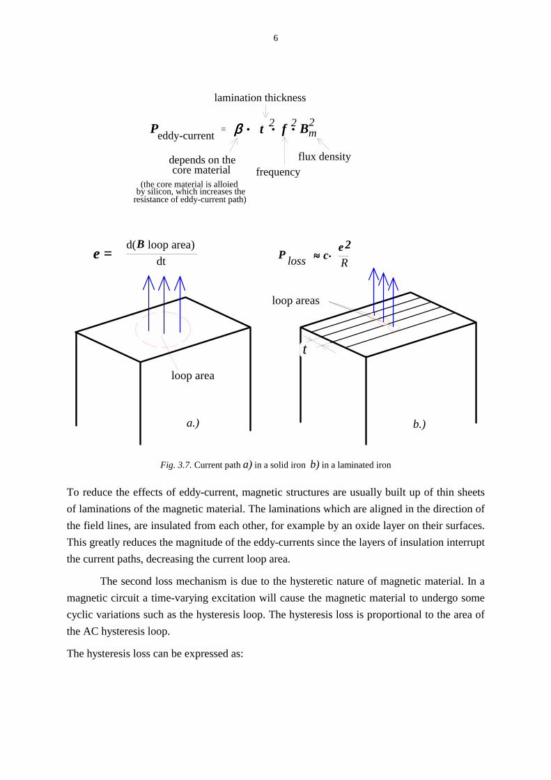
Peddy-current Bm2. ..

lamination thickness

core materialdepends on the

(the core material is alloiedby silicon, which increases the

resistance of eddy-current path)

frequencyflux density

f 2t 2ββββ=

e = d( loop area)dt

loop area

loop areas

P loss ~~ c eR2

~ .

a.)

t

B

b.)

Fig. 3.7. Current path a) in a solid iron b) in a laminated iron

To reduce the effects of eddy-current, magnetic structures are usually built up of thin sheets of laminations of the magnetic material. The laminations which are aligned in the direction of the field lines, are insulated from each other, for example by an oxide layer on their surfaces. This greatly reduces the magnitude of the eddy-currents since the layers of insulation interrupt the current paths, decreasing the current loop area.

The second loss mechanism is due to the hysteretic nature of magnetic material. In a magnetic circuit a time-varying excitation will cause the magnetic material to undergo some cyclic variations such as the hysteresis loop. The hysteresis loss is proportional to the area of the AC hysteresis loop.

The hysteresis loss can be expressed as:

7

P hysterezis Bm(1,6...2)..

frequencyflux density

fαααα=

the core material

a coefficientdepending on

Because the magnetic material undergoes f times a cycle in a second the hysteresis loss is proportional to frequency f.

In general, the losses depend on the metallurgy of the material as well as the flux density. A frequency information on core loss is measured and typically presented in graphical form. It is plotted in terms of watts per unit weight as a function of flux density (Fig. 3.6).

Nearly all transformers and electric machines use sheet-steel material that has high favourable directions of magnetization along the core. Loss is low and the permeability is high. The material is called grain-oriented steel.

Returning to the transformer, to reduce the iron-core losses is the reason of the core laminations. Two common types of construction are illustrated in Fig. 3.9.

In the core type the windings are wound around two legs of a rectangular magnetic core; while in the shell type core the windings are wound around the center leg of a three-legged core. Silicon-steel laminations of 0.035 cm (approximately. 4 per cent silicon is alloyed to the steel) are generally used for transformers operating at frequencies below a few hundred Hertz’s. Silicon steel has the desirable properties of low cost, low core loss and high permeability at high flux densities (1.0 to 1.5 T). The cores of small transformers used in

a.)core type shell type

primary

secondary

core ϕ

leg

tt 2 t 2

primarywindings

b.)

secondarywindings

2ϕ

2ϕ

Fi

g. 3.9. Common types of transformer construction

8

communication circuits at high frequencies and low energy levels are sometimes made of compressed powdered ferromagnetic alloys such as permalloy.

Most of the flux is confined to the core and therefore links both windings. It is the main or mutual flux. The other is a small fraction of the total flux, which links one winding without linking the other. It is the leakage flux. The leakage flux has an important effect on the behaviour of the transformer. Leakage is reduced by subdividing the windings into

sections placed as close together as possible. In the core-type construction, each winding consist of two section, one section on each of the two legs of the core; the primary and secondary windings are concentric coils. In the shell-type construction the windings consist of a number of thin "pancake" coils assembled in a

stack with primary and secondary coils interleaved.

3.1 THE EQUIVALENT CIRCUIT

A transformer is illustrated in Fig. 3.11., but let the properties of this transformer windings idealized.

It means that: • the resistances of windings were taken out and separately drawn; • the reactances which are corresponded to the leakage flux of windings were

taken out and separately drawn. It is named as leakage inductance. • the magnetizing current (which is required to produce the main flux) depends on

the emf (or the flux density) and is lagging emf by 90°, therefore we take it into account as a shunt reactance, Xm.

• the core losses are wattous losses which are in phase with and dependent on the emf, therefore we take they into account as a shunt resistance, Rc.

The idealized transformer is illustrated in Fig. 3.11.

ϕ (t) (main flux)

leakage fluxϕ l1

ϕ l2N1 N2

secodarywinding

primarywinding

Fig. 3.10. The main and leakage flux lines

9

R X

R X

NE

NE

X R

ZV V

1 l1

c m

l2 2

1 2 t1

1

2

2

idealized transformer

I I

I

II

I1

cm

2 2

ϕϕϕϕ

i = magnetizing currenti = core-loss currentmc

'

Fig. 3.11. The idealized transformer

The induced voltage in the windings:

E N ddt

E N ddt1 1 2 2= ⋅ = ⋅ϕ ϕ and

The voltage ratio, a:

a EE

NN

= =1

2

1

2

Thus the transformational ratio is directly proportional to the ratio of the winding numbers.

Now let a load be connected to the secondary winding. A current I2 and an mmf (exciting) N2I2 are then present in the secondary winding. Because the core flux mustn't change, in the primary winding there must be produced a compensating mmf as:

N I N I1 2 2 2⋅ = ⋅' ,

where:

I NN

I Ia2

1

2

221' = ⋅ =

thus a transformer changes currents in inverse ratio of the turns in its windings.

Because the two windings are isolated from each other we can link them in a point.

10

idealized referred transformer

R X

R X

NE

NE

X R

ZV V

1 l1

c m

l2 2

1 2 t1

1

2

2

I I

I

II

I1

cm

2 2

ϕϕϕϕ

' '' '

''' E1=

Fig. 3.12. Idealized, referred transformer

If we replace the secondary (which has N2 turns) with a new winding which has N1 turns as much as the primary, in both windings same voltage will be induced:

E E NN

E a2 21

22

' = =

where E2' is the referred voltage E2 to the primary; it is in direct ratio to the voltage ratio.

This is the first step in a transformation because we would replace the secondary with referred parameters (Fig. 3.12.).

Because at a referred transformers in the primary and secondary turns the voltages are same, the role in the idealized transformer is only to produce the induced voltage E1=E'2 and the excitation compensation. Thus the idealized transformer can be replaced with a E1=E'2 voltage on the shunt Rc resistance and Xm reactance, and with a i'2 current which solves the excitation compensation:

R X

R X

R

V

1 l1

c m1

I

I

I I

1

c m

ϕϕϕϕ

Zt

Xl2 2I2

V2

'

' '

' '

1E2' E=

Fig. 3.13. The equivalent T circuit of a transformer

We hasn't discussed yet the impedance transformation. Because the energy loss is constant at the transformation we can write for a resistance:

11

beforereferring

.,I 2

2 .I 22 R2

2=,

R22

afterreferring

Then:

R II

R22

2

2

2'

'=

⋅

the current transformation is in inverse proportion to the voltage ratio, therefore

R a R22

2' = ⋅

Also the resistance such the reactance transformation is in direct ratio squared.

X a Xl l22

2' = ⋅

This equation shows the impedance-transformation ability of a transformers.

Transferring an impedance from one side of a transformer to the other is called referring the impedance to the other side. In a similar way, voltages and currents can be referred to one side with transformation rules to evaluate the equivalent parameters on that side.

To sum up, in an ideal transformer voltages are transformed in direct ratio of turns, currents in the inverse ratio, the impedances in the direct ratio squared; power volt-amperes and excitation are unchanged.

For practice and understanding the behaviour of a transformer the equivalent circuit parameters are given for a middle-power transformer in Fig. 3.14.:

R X

R X

R1 l1

c m

Xl2 2' '

111 111112112

104 103

12

Fig. 3.14. Equivalent circuit parameters for a middle-power transformer

3.2. OPERATING MODES AND PHASOR DIAGRAMS OF THE TRANSFORMERS

Two very simple tests serve to determine the constants of the equivalent circuit.

3.2.1. OPEN CIRCUIT TEST AND WORKING MODE

The measuring connection of the open circuit test of a three phase transformer is illustrated in Fig. 3.15., during the test the secondary is open circuited.

A

A

A

RST

TORROIDTRANSFORMER

supply

threephase

system v

v

v

A

B

C

W

W

a

b

c

V

MEASUREDTRANSFORMER

Fig. 3.15. The open-circuited test

Because the secondary is open circuited, the secondary referred current I'2=0, also the equivalent circuit is shown in Fig. 3.16.:

R X

R XV

1 l1

c m1

I

i

i i

1

c m

ϕϕϕϕ

I 2'

1E2' E=

= 0

Fig. 3.16. The equivalent circuit when the secondary is open circuited

In the equivalent circuit the currents and the voltages are phasors. Based on the following expression the phasor diagram for no-load is illustrated in Fig. 3.17. :

V I R j I X El1 1 1 1 1 1= + +

With the secondary open circuited and rated voltages is impressed on the primary, the exciting current is only 2 to 6 percent of full-load current. For convencience, the lower

13

voltage side is usually taken as the primary in this test. The voltage drop in the primary resistance and leakage reactance is entirely negligible, and the primary impressed voltage V1

nearly equals the emf E1 induced by the resultant core flux. Also the primary I2R loss caused by the exciting is entirely negligible, so that the power input P1 very nearly equals the core loss Pc.

Thus we can determine the shunt parts in the equivalent circuit with the open circuit test. The core-loss component is:

R PUc ≈ 1

12

The shunt impedance is:

Z UIS ≈ 1

ϕ

Therefore Xm is:

X Z Rm S c= −2 2

The values so obtained are of course referred to the side which was used as the primary in the test. Sometime the voltage on the terminals of the open-circuited secondary is measured as a check on the turn ratio.

During open circuited test we can measure the open circuit characteristics ( P0, Iϕ, cosϕ versus E1) which are illustrated in Fig. 3.18.

The Poc (which is the core-losses) versus E1 characteristic approximately is a parabola because both hysteresis and eddy current core losses are in direct ratio squared of the magnetic flux density which is proportional to emf E1. The Iϕ characteristic a H(B) magnetizing curve because the Iϕ is basically the core magnetizing current which proportional to H and Bm is proportional to E1 = 4.44.f.N.Bm.Ac. The power factor is low, the current Iϕ is lagging by nearly 90°.

ϕ

U1 E =E1

i R

ji X

i

i m

i c

ϕ

1

1 l1

2

U =i R +ji X +E1 1 1 l1 11

cos ~ 0.17ϕϕϕϕ ~

'

Fig. 3.17. The open circuit phasor

diagram

14

3.2.1. THE SHORT-CIRCUIT TEST

With the secondary is short circuited, typically a primary voltage only 2..12 percent of the rated value need to be impressed to obtain full-load current. For convenience the high-voltage side is usually taken as the primary in this test. Because the impressed voltage is on

very low level the exciting current and core losses entirely negligible, the shunt part in the equivalent circuit can then be omitted. The equivalent circuit is shown in Fig. 3.19.:

The power input nearly equal to the total I2R loss in the primary and secondary windings, and the impressed voltage equal to the drops in the summed primary and secondary resistance and leakage reactance.

The short circuit impedance, resistance and reactance are (all parameter are measured at rated current!):

ZU

I

R PI

X Z R

scsc

sc

scsc

sc

sc sc sc

=

=

= −

2

2 2

We can define the drop and it's components by the means of the short-circuited test. The voltage drop at rated current is:

P = P0 c

Iϕ

E1rated

P

parabola

cosϕ

cosϕ oc

Iϕmagnetizing

curve

V1 ~ E0

c B. m

~ 0,15

Fig. 3.18. The open circuit characteristics of a transformer

Vsc

Rsc = R 21 + R ' Xsc = X l1 + X 'l2

Isc = I 1

Zsc

Fig. 3.19. The equivalent circuit for short-circuit

15

ε zsc

r

VV

= ,

where Vsc is the voltage drop in the short-circuited impedance at rated current. The drop of a transformer is from 2 to 10 percent, the drop of a smaller transformer is higher. The drop components are:

εRR,sc

r

VV

= and ε XX,sc

r

VV

=

When in the equivalent circuit the shunt branch is omitted, the approximate values of the individual primary and secondary resistances and leakage reactances can be obtained by assuming that R1 = R2 = 0.5.Rsc and Xl1 = Xl2 = 0.5.Xsc.

The short-circuit phasor diagram and steady-state characteristics are illustrated in Fig. 3.20. and fig. 3.21.:

U U U I R j I Xsc Xsc Rsc sc sc sc sc= + = ⋅ + ⋅ ⋅

The short circuit characteristics are: the input power Psc, the impressed voltage Vsc on the transformer terminal and the

power factor cosϕsc versus Isc. The Psc characteristic is a parabola because it is the summed power losses (I2sc.Rsc) in the windings. In the short-circuited test the magnetic circuit is unsaturated, the impedance Zsc is constant, i.e. the Usc characteristic versus Isc is a line. The power factor is

U

Usc

Xsc

URsc

scI

cos ~0.4..0.5ϕϕsc

U U U I R j I Xsc Xsc Rsc sc sc sc sc= + = ⋅ + ⋅ ⋅

Fig. 3.20. The phasor diagram in short circuit.

P sc

I scrated

parabola

cosϕ

cosϕ sc

~ 0,45

P = Psc w

U sc

I sc

U sc

Fig. 3.21. The short circuit characteristics of a transformer

16

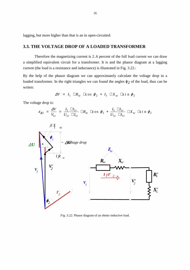
lagging, but more higher than that is an in open-circuited.

3.3. THE VOLTAGE DROP OF A LOADED TRANSFORMER

Therefore the magnetizing current is 2..6 percent of the full load current we can draw a simplified equivalent circuit for a transformer. It is and the phasor diagram at a lagging current (the load is a resistance and inductance) is illustrated in Fig. 3.22.:

By the help of the phasor diagram we can approximately calculate the voltage drop in a loaded transformer. In the right triangles we can found the angles ϕ2 of the load, thus can be writen:

∆V I R I Xsc sc= ⋅ ⋅ + ⋅ ⋅1 2 1 2c os s i nϕ ϕ

The voltage drop is:

ε ϕ ϕϕ21

1 1

1 12

1 1

1 12= = ⋅

⋅⋅ ⋅ + ⋅

⋅⋅ ⋅∆V

VI I

U IR I I

U IX

r

r

r rsc

r

r rscc os s i n

R X

R'

X'

sc sc

L

L

V1V'2

I'2

jI X1 sc

2ϕϕϕϕ

2ϕϕϕϕ

U∆~ voltage drop

V'2

I =I'1 2

Zsc

U∆

I R1 sc....

V1

Fig. 3.22. Phasor diagram of an ohmic-inductive load.

17

and then with the drop-component:

( )ε ε ϕ ε ϕϕ21

12 2= ⋅ + ⋅I

I rR sc os s i n

or in an other way expressed:

( )ε ε ϕ ϕϕ21

12= −I

I rz s cc os ,

where the ϕsc is the phasor angle of the short-circuited impedance. The output voltage is:

( )U U r2 2 21' '= ⋅ − εϕ

To sum up: the voltage drop in a loaded transformer proportional to the current and the drop and depend on the phase angle of the load.

The Fig. 3.23. illustrates the voltage drop characteristic at a constant load current as a function of the power factor.

The relationship between voltage drop and load volt-amperes illustrated in Fig. 3.24.

3.4. THE EFFICIENCY OF A

TRANSFORMER

The efficiency is:

η

ϕϕ

= = =+

=

=+ +

powe rpowe r

PP

PP l os s e s

U IU I P Pc w

out put i nput

2

1

2

2

2 2 2

2 2 2

c osc os

,

where Pw =I22.R is the winding losses, Pc is the core losses. Division by I2 then is given:

V2r

capacitiveload

Inductiveload

∆V

cos 2ϕ

V2

-

+

Fig. 3.23. The voltage drop of a transformer at constant current

as a function of the power factor

V2

V20εz1

εz2

ε > εz2 z1

S

Fig. 3.24. The voltage drop of a transformer at constant power factor

as a function of load Volt-Amperes

18

η ϕ

ϕϕ

=+ +

=+ ∑

U

U PI

I R LS

c

r

2 2

2 22

2

2

1

1

c os

c osc os

where ΣL is summed losses, Sr the rated volt-amperes.

The efficiency is the maximum, if the

PI

I Rc

22+

member is the minimum versus load.

The minimum value can be obtained if:

a l s o - Pc

d PI

I R

dIPI

R I R P

c

cw

22

2

22 2

2

0

0

+

=

+ = ⇒ = ⋅ =

We can see that, the efficiency of a transformer is the maximum, if the core losses are equal to the winding losses. Efficiency of a power transformer is normally 90..95%. The relationship between the efficiency η and the load volt-amperes S are illustrated in Fig. 3.25.:

~ 0.95

η

SP = Pc w

cos = 1,0ϕ, %

cos = 0,8ϕ

Fig. 3.25. The transformer efficiency-load volt-amperes relationship.

19

3.5. THE THREE-PHASE TRANSFORMERS

tt t

h

flux lines secondary

primary

Fig. 3.26. The construction of a core type three-phase transformer.

Three single phase transformers can be connected to form a 3-phase bank. Instead of three single phase transformers a 3-phase bank may consist of one 3-phase transformer having all six windings on a common multilegged core and contained in a single bank. In Fig. 3.26. we can see a core type (three legged) transformer.

At the core type 3-phase transformer has a primary and secondary windings on all legs. There is a difference between the lengths of the flux lines of phases, the excitation length of the middle phase is shorter than of two outside phases. Therefore the magnetizing currents are different too, the current of the middle phase is smaller.

The windings of a 3-phase transformer with a balanced load may be connected to or ∆, the -∆ connection is commonly used in stepping down from a high voltage to a

medium or a low voltage. Because in most cases a neutral is provided for ground on the high voltage side the high voltage side usually is in a star connection with a neutral conductor. Thus the ∆- is commonly used for stepping up to a high voltage.

There is some very important notice when we use a 3 phase transformer and we would like to determine the parameters for the equivalent circuit: in an equivalent circuit all voltages, currents, resistances and reactances are phase-quality. The measured power is a 3-phase power, therefore must divide by 3, and must take the line and phase differences into account. The used voltage ratio must be calculated from phase voltages.

20

A

C

B

i A

A B C

V V

V

CA AB

BC

V

V VC B

Ai B

iB

VAB VBC

VCA

A

BC

VA VB VC

Fig. 3.27. The star-connection of the windings.

For example in star connection which is illustrated in Fig. 3.27 the UA,UB,UC voltages are phase-quantities, the UAB,UBC,UC voltages are line-quantities, thus:

( ) ( )U U U U U U U UL AB BC CA phas e A B C( ) ( ), , , ,= ⋅3

i.e. the line-voltage quantities are 3 (three square rooted) times greater than the phase-voltage quantities:

U Ul i ne phas e( ) ( )= ⋅3

The phase- and the line-current quantities in a star connection are equal to each other:

I Il i ne phas e( ) ( )=

The three-phase power is:

S U I U Iphas e phas e l i ne l i ne= =3 3( ) ( ) ( ) ( )

A delta connection is shown in Fig. 3.28.

AC BA B C

V V

V

CA AB

BC

I

phAI

L

C BA

IphC

Fig. 3.28. The delta connection of the transformer windings.

21

In delta connection the line and phase voltages are equal to each other:

U Ul i ne phas e( ) ( )= ,

but the line currents are 3 times greater than the phase currents:

I Il i ne phas e( ) ( )= ⋅3

The 3-phase volt-amperes in this case is:

S U I U Iphas e phas e l i ne l i ne= =3 3( ) ( ) ( ) ( )

3.6. THE PHASE SHIFT OF A TRANSFORMER

V

V VC B

A V

V Vc b

a

Fig. 3.29. A Yoyo0 connected transformer.

Shall we now assume a transformer, which is connected as illustrated in Fig. 3.29.

The transformer connections are standardised, marked with two letters followed number. The connection of windings are described by letters (the primary is marked by upper case letter, the secondary is marked by lower case letter), the number describes the phase shift in hour (each hour is 30° phase shift). For the transformer illustrated in Fig. 3.29. the standardised marking is Yoyo0, because this transformer hasn't got any phase-shift, it means that the phase "A" voltage on the primary terminals are in phase with the phase "a" voltage on the secondary terminals (if there is a neutral line, it is marked with 0 in index).

Next shall we see the transformer in Fig. 3.30! If we compare the connection of windings with the transformer connection examined before, we can see that at this transformer the secondary neutral connection is interchanged:

A B C

a b c n

N

The point makesthe beginningof the windingson a core leg.

22

A B C

a b c n

N

VA

Va

VA

Va

ωωωω

VC VB

VbVc

0

3

6

9

Fig. 3.30. The Yoyo6 transformer.

Based on the shown phasor diagrams we can see that the neutral-connection changing for an Yy connected transformer causes 180° phase-shift, it is marked by number 6.

A B C

a b c

VAB

VBC

VCA

VAB

Va

n

Vb Vc

Vab

VabDy 110

Va

11

12

Fig. 3.31. A Dyo5 transformer connections.

Shall we see next a Dy transformer, which is illustrated in Fig. 3.31.

3.7. THE PARALLEL CONNECTION OF THE TRANSFORMERS

23

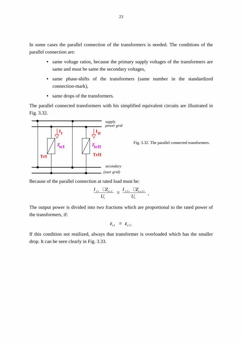
In some cases the parallel connection of the transformers is needed. The conditions of the parallel connection are:

• same voltage ratios, because the primary supply voltages of the transformers are same and must be same the secondary voltages,

• same phase-shifts of the transformers (same number in the standardized connection-mark),

• same drops of the transformers.

The parallel connected transformers with his simplified equivalent circuits are illustrated in Fig. 3.32.

Fig. 3.32. The parallel connected transformers.

Because of the parallel connection at rated load must be:

I ZU

I ZU

I r s c I

r

I I r s c I I

r

⋅ = ⋅ ,

The output power is divided into two fractions which are proportional to the rated power of the transformers, if:

ε εz I z I I=

If this condition not reailized, always that transformer is overloaded which has the smaller drop. It can be seen clearly in Fig. 3.33.

Z Z

I I

TrI TrII

I II

scI scII

supplypower grid

secondary(user grid)

24

V20

I

SIS

III

II III I I

I

U∆∆∆∆voltagedrop of thetransformers

εεεε

>ε>ε>ε>εzII zI

Fig. 3.33. The load distribution for parallel connected transformers with different drops