transient signal analysis - national physical...
TRANSCRIPT
1
Good Practice in Signal Processing: case study on the use of signal processing techniques in the analysis of environmental
vibration data
Xiangqian Jane Jiang, Wenhan Zeng and Paul Scott, University of Huddersfield Francois Maletras, Ian Smith and Trevor Esward, National Physical Laboratory
1 Introduction
This report describes the application of a number of signal processing techniques to environmental vibration measurements recorded by the Watt balance team at the National Physical Laboratory.
1.1 Basic features of the measurement data The main features of the measurement data are as follows:
1. A single measurement cycle lasts 20 minutes and involves taking measurements using seven sensors in different locations, with no overlap in time between any of the measurements.
2. The sampling frequency is 250 Hz and each sensor records 214 = 16,384 samples over a period of just over 65.5 seconds.
3. For each of the seven sensors (name and order: accel0, accel0diffaccel2, accel2, accel2diffaccel3, accel3, accel0diffaccel3 and bruel), 252 data sets have been recorded over a period of 3.5 days.
1.2 Signal processing aims This report describes methods and algorithms for five tasks:
1. To identify non-stationary signals using time domain analysis.
2. To investigate the frequency structure of the signals.
3. To identify non-stationary signals using wavelet analysis (and compare results with those obtained using time domain analysis).
4. To use wavelet analysis to identify the time location of transient events in signals.
5. To use wavelet denoising methods to extract transient events in signals.

2 Time domain analysis
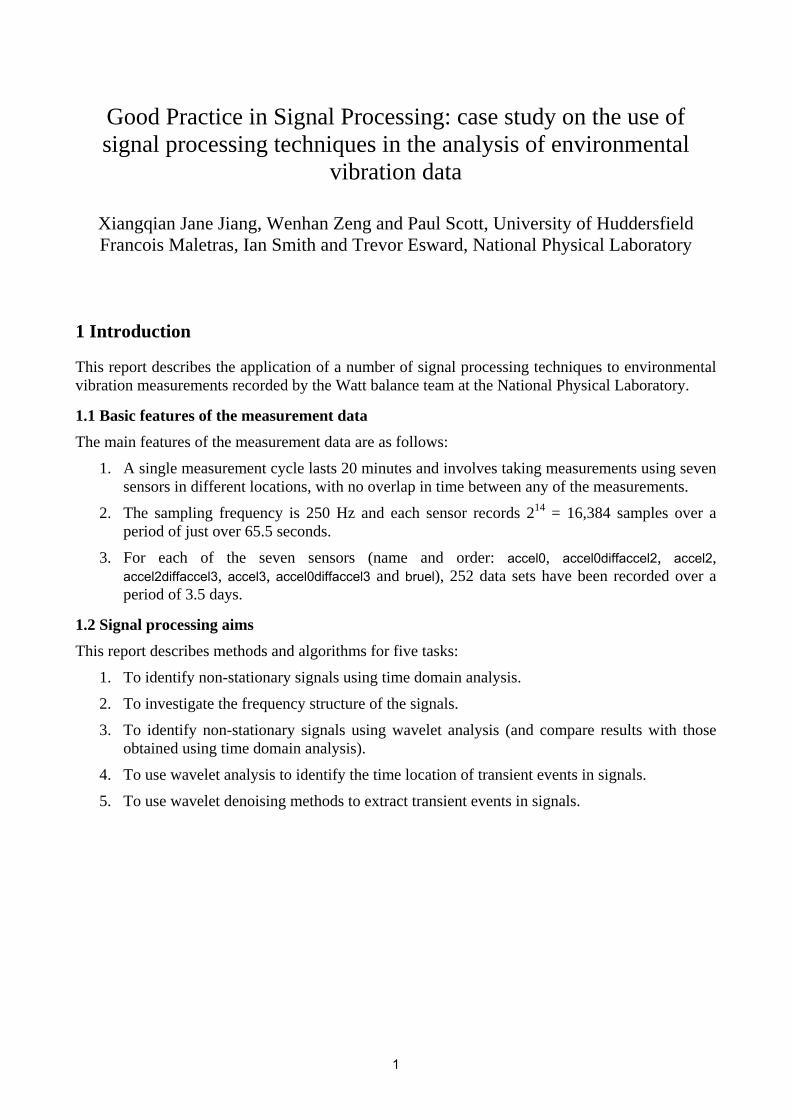
For each sensor, a simple statistical method, short-time analysis, is used to explore all the datasets and try to identify those datasets that potentially contain transient events as follows.
qP
The value of a portion of a dataset is the root mean square of the signal values within that portion. In the jth portion of the ith dataset, is defined as
qP),( jiPq
,1),(1
2∑=
=m
kkq z
mjiP
where m is the length (number of points) of the portion and is the kth signal value within that portion.
kz
For the dataset, the ratio
),(min
),(max)(
jiP
jiPir
qj
qjPq
=
is calculated. Assuming that transient events are followed by an abrupt change in amplitude, a large value of shows a high probability of the existence of transient events in the dataset. A simple method of identifying datasets that possibly contain transient events is to consider only those datasets whose
values are greater than some threshold value.
qPr
qPr
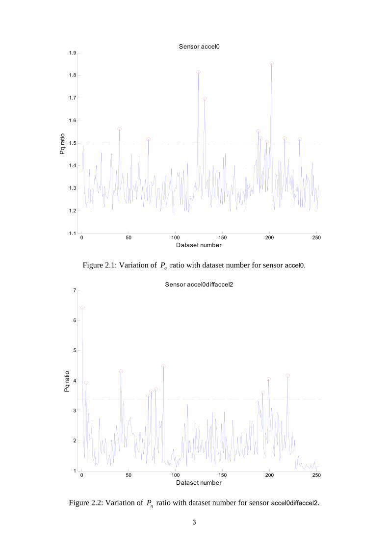
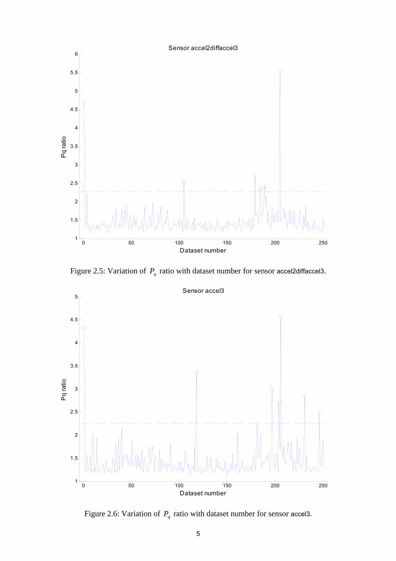
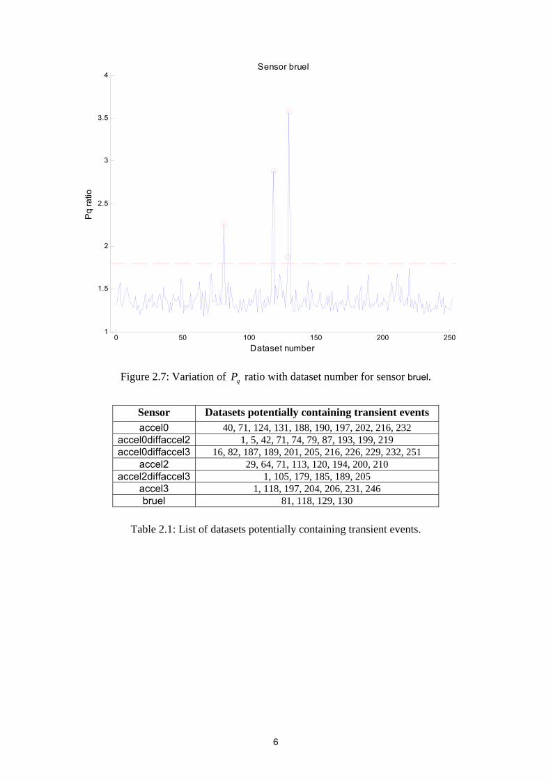
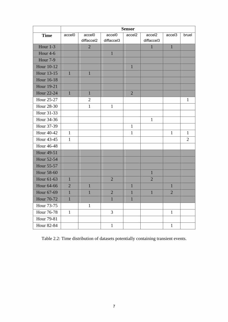
Figures 2.1 to 2.7 show, for each sensor, the results of the short-time analysis. In all cases, the short-time window contains 512 points (corresponding to a time interval of 2.048 seconds). The threshold value is denoted by the red dotted line and is set to be the mean of all the values plus two times their standard deviation. Red circles are used to indicate those datasets identified by the thresholding process as potentially containing transient events.
qP
qPr
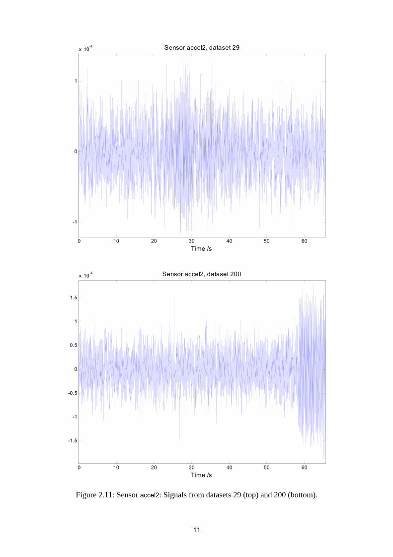
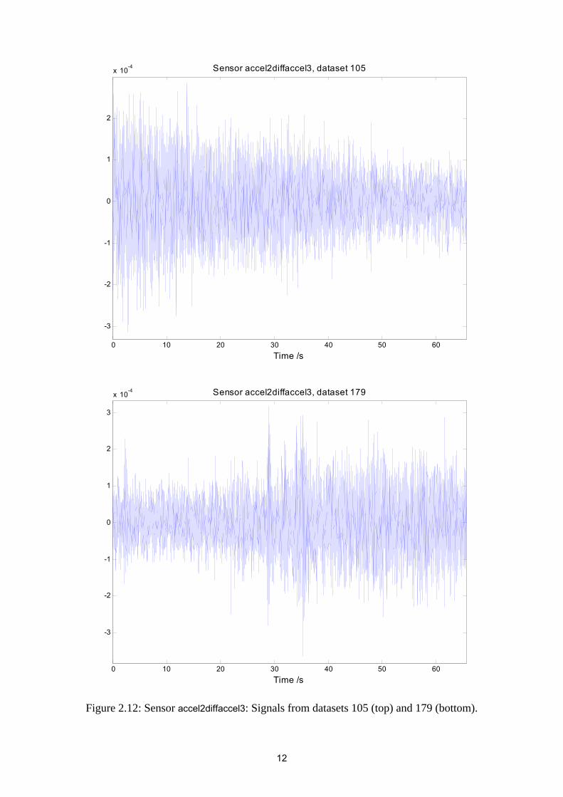
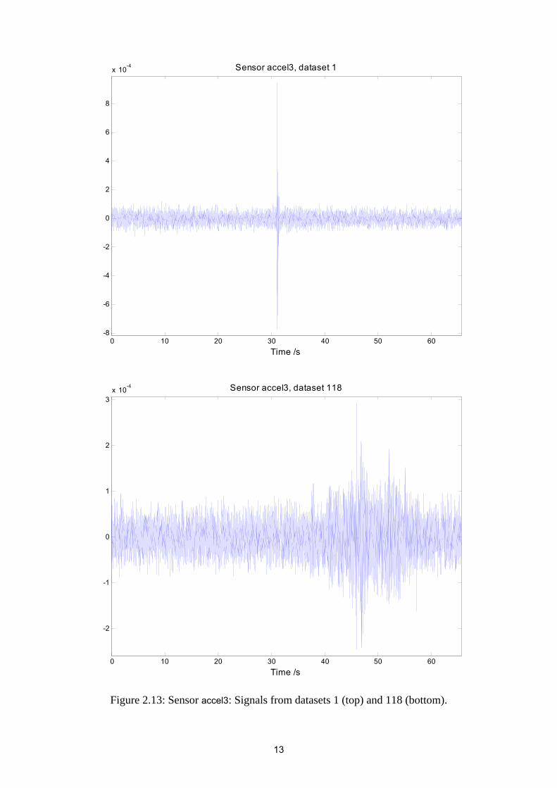
Table 2.1 lists the datasets identified by the thresholding process while table 2.2 illustrates the distribution in time of the identified datasets. It is interesting to note that for each of the six sensors accel0, accel0diffaccel2, accel0diffaccel3, accel2, accel2diffaccel3 and accel3, a number of transient events are identified as potentially occurring around dataset 200. Visual examination of the signals shows that there are indeed transient events in all identified signals and that short-time analysis is effective in allowing the user to identify signals of interest. It should be noted that the accuracy of the analysis depends both on the size of the window used and the criteria used for thresholding.
qP
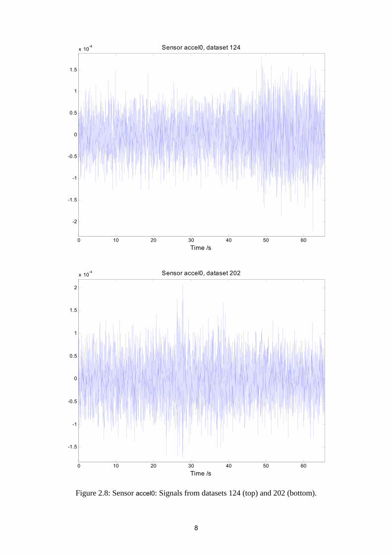
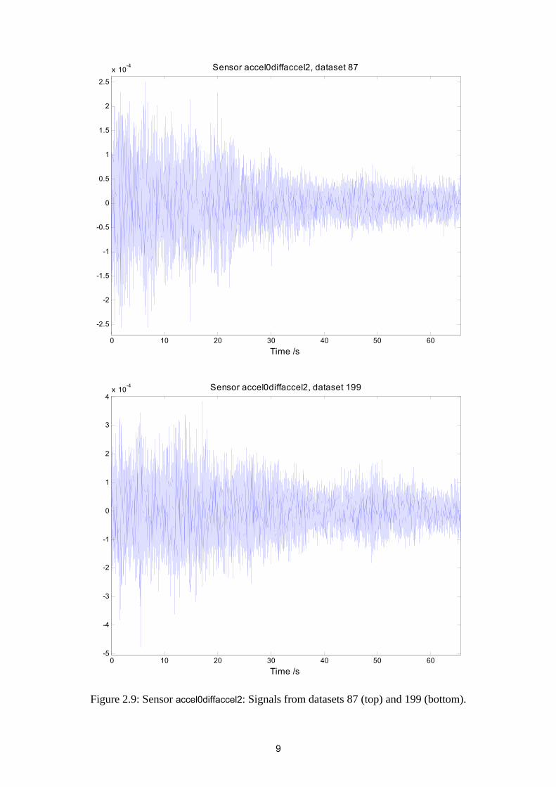
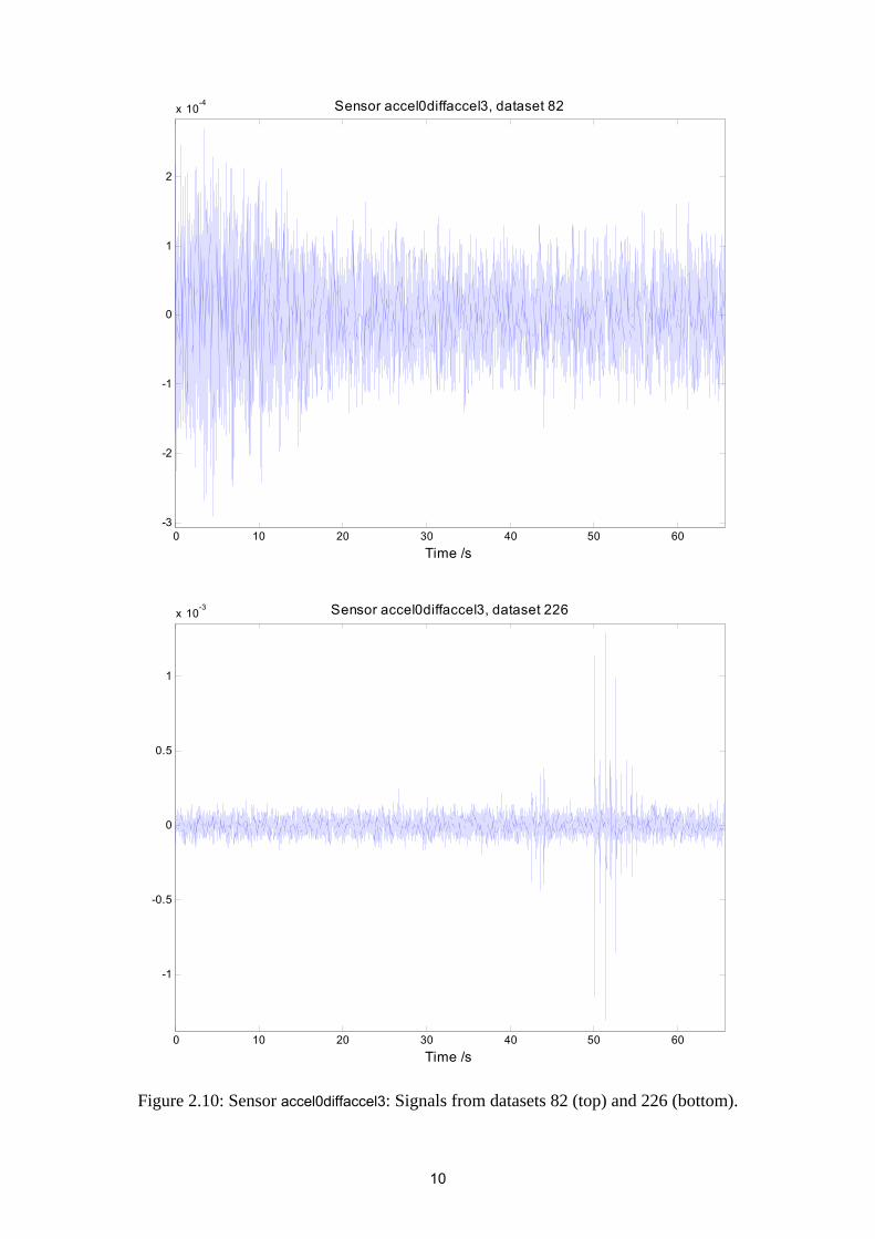
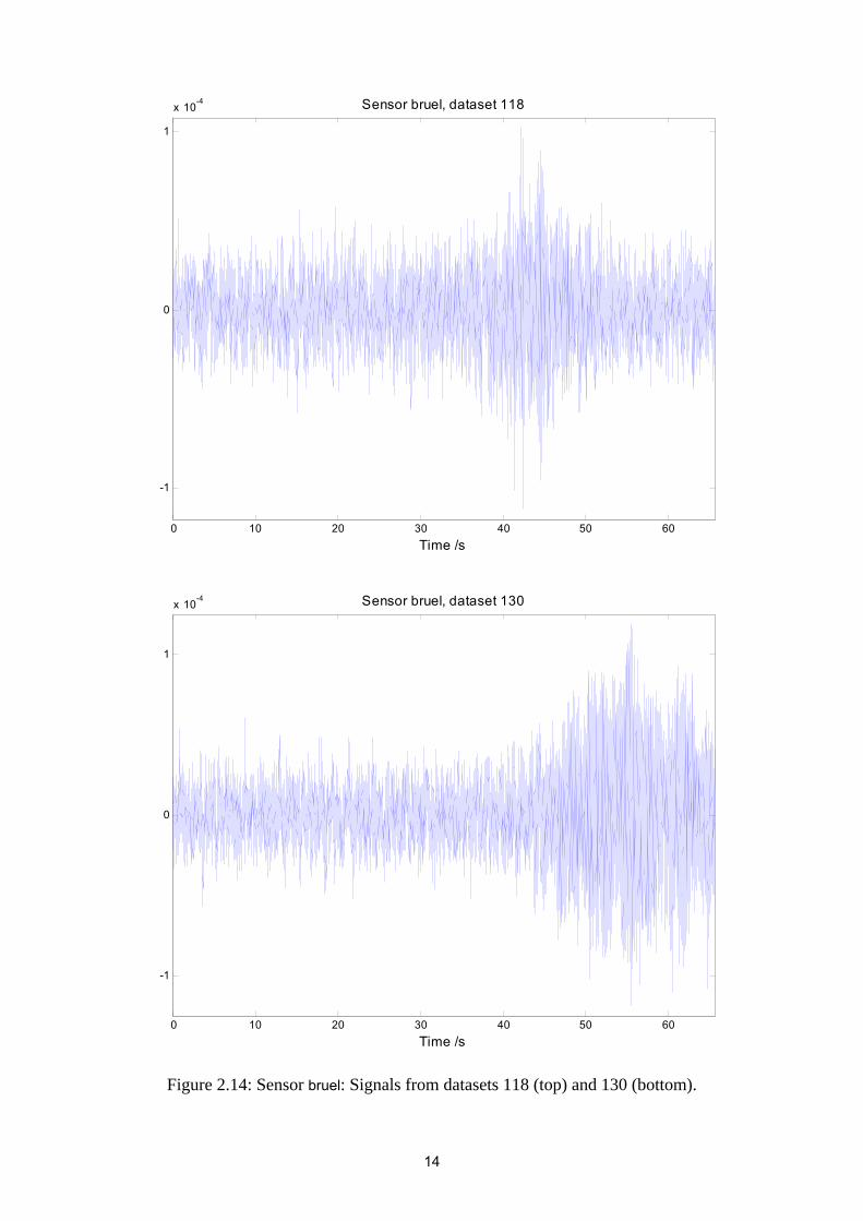
From the list of datasets in table 2.1, two datasets have been randomly selected for each sensor. The signals from these datasets are displayed in figures 2.8 to 2.14.
2
0 50 100 150 200 2501.1
1.2
1.3
1.4
1.5
1.6
1.7
1.8
1.9
Dataset number
Pq
ratio
Sensor accel0
Figure 2.1: Variation of ratio with dataset number for sensor accel0. qP
0 50 100 150 200 2501
2
3
4
5
6
7
Dataset number
Pq
ratio
Sensor accel0diffaccel2
Figure 2.2: Variation of ratio with dataset number for sensor accel0diffaccel2. qP
3

0 50 100 150 200 2501
1.5
2
2.5
3
3.5
4
Dataset number
Pq
ratio
Sensor accel0diffaccel3
Figure 2.3: Variation of ratio with dataset number for sensor accel0diffaccel3. qP
0 50 100 150 200 2501
1.2
1.4
1.6
1.8
2
2.2
2.4
2.6
2.8
3
Dataset number
Pq
ratio
Sensor accel2
Figure 2.4: Variation of ratio with dataset number for sensor accel2. qP
4
0 50 100 150 200 2501
1.5
2
2.5
3
3.5
4
4.5
5
5.5
6
Dataset number
Pq
ratio
Sensor accel2diffaccel3
Figure 2.5: Variation of ratio with dataset number for sensor accel2diffaccel3. qP
0 50 100 150 200 2501
1.5
2
2.5
3
3.5
4
4.5
5
Dataset number
Pq
ratio
Sensor accel3
Figure 2.6: Variation of ratio with dataset number for sensor accel3. qP
5
0 50 100 150 200 2501
1.5
2
2.5
3
3.5
4
Dataset number
Pq
ratio
Sensor bruel
Figure 2.7: Variation of ratio with dataset number for sensor bruel. qP
Sensor Datasets potentially containing transient events accel0 40, 71, 124, 131, 188, 190, 197, 202, 216, 232
accel0diffaccel2 1, 5, 42, 71, 74, 79, 87, 193, 199, 219 accel0diffaccel3 16, 82, 187, 189, 201, 205, 216, 226, 229, 232, 251
accel2 29, 64, 71, 113, 120, 194, 200, 210 accel2diffaccel3 1, 105, 179, 185, 189, 205
accel3 1, 118, 197, 204, 206, 231, 246 bruel 81, 118, 129, 130
Table 2.1: List of datasets potentially containing transient events.
6
7
Sensor
Time accel0 accel0 diffaccel2
accel0 diffaccel3
accel2 accel2 diffaccel3
accel3 bruel
Hour 1-3 2 1 1 Hour 4-6 1 Hour 7-9
Hour 10-12 1 Hour 13-15 1 1 Hour 16-18 Hour 19-21 Hour 22-24 1 1 2 Hour 25-27 2 1 Hour 28-30 1 1 Hour 31-33 Hour 34-36 1 Hour 37-39 1 Hour 40-42 1 1 1 1 Hour 43-45 1 2 Hour 46-48 Hour 49-51 Hour 52-54 Hour 55-57 Hour 58-60 1 Hour 61-63 1 2 2 Hour 64-66 2 1 1 1 Hour 67-69 1 1 2 1 1 2 Hour 70-72 1 1 1 Hour 73-75 1 Hour 76-78 1 3 1 Hour 79-81 Hour 82-84 1 1
Table 2.2: Time distribution of datasets potentially containing transient events.
0 10 20 30 40 50 60
-2
-1.5
-1
-0.5
0
0.5
1
1.5
x 10-4
Time /s
Sensor accel0, dataset 124
0 10 20 30 40 50 60
-1.5
-1
-0.5
0
0.5
1
1.5
2
x 10-4
Time /s
Sensor accel0, dataset 202
Figure 2.8: Sensor accel0: Signals from datasets 124 (top) and 202 (bottom).
8
0 10 20 30 40 50 60
-2.5
-2
-1.5
-1
-0.5
0
0.5
1
1.5
2
2.5
x 10-4
Time /s
Sensor accel0diffaccel2, dataset 87
0 10 20 30 40 50 60-5
-4
-3
-2
-1
0
1
2
3
4x 10
-4
Time /s
Sensor accel0diffaccel2, dataset 199
Figure 2.9: Sensor accel0diffaccel2: Signals from datasets 87 (top) and 199 (bottom).
9
0 10 20 30 40 50 60-3
-2
-1
0
1
2
x 10-4
Time /s
Sensor accel0diffaccel3, dataset 82
0 10 20 30 40 50 60
-1
-0.5
0
0.5
1
x 10-3
Time /s
Sensor accel0diffaccel3, dataset 226
Figure 2.10: Sensor accel0diffaccel3: Signals from datasets 82 (top) and 226 (bottom).
10
0 10 20 30 40 50 60
-1
0
1
x 10-4
Time /s
Sensor accel2, dataset 29
0 10 20 30 40 50 60
-1.5
-1
-0.5
0
0.5
1
1.5
x 10-4
Time /s
Sensor accel2, dataset 200
Figure 2.11: Sensor accel2: Signals from datasets 29 (top) and 200 (bottom).
11
0 10 20 30 40 50 60
-3
-2
-1
0
1
2
x 10-4
Time /s
Sensor accel2diffaccel3, dataset 105
0 10 20 30 40 50 60
-3
-2
-1
0
1
2
3
x 10-4
Time /s
Sensor accel2diffaccel3, dataset 179
Figure 2.12: Sensor accel2diffaccel3: Signals from datasets 105 (top) and 179 (bottom).
12
0 10 20 30 40 50 60-8
-6
-4
-2
0
2
4
6
8
x 10-4
Time /s
Sensor accel3, dataset 1
0 10 20 30 40 50 60
-2
-1
0
1
2
3x 10
-4
Time /s
Sensor accel3, dataset 118
Figure 2.13: Sensor accel3: Signals from datasets 1 (top) and 118 (bottom).
13
0 10 20 30 40 50 60
-1
0
1
x 10-4
Time /s
Sensor bruel, dataset 118
0 10 20 30 40 50 60
-1
0
1
x 10-4
Time /s
Sensor bruel, dataset 130
Figure 2.14: Sensor bruel: Signals from datasets 118 (top) and 130 (bottom).
14
15
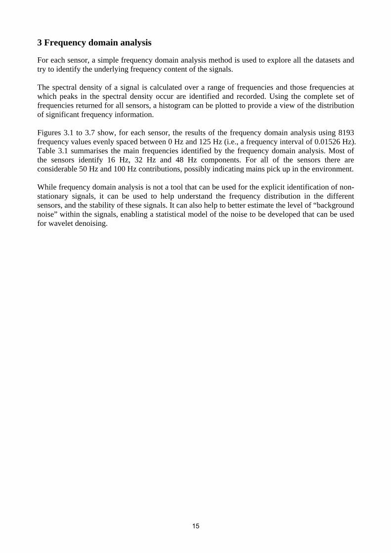
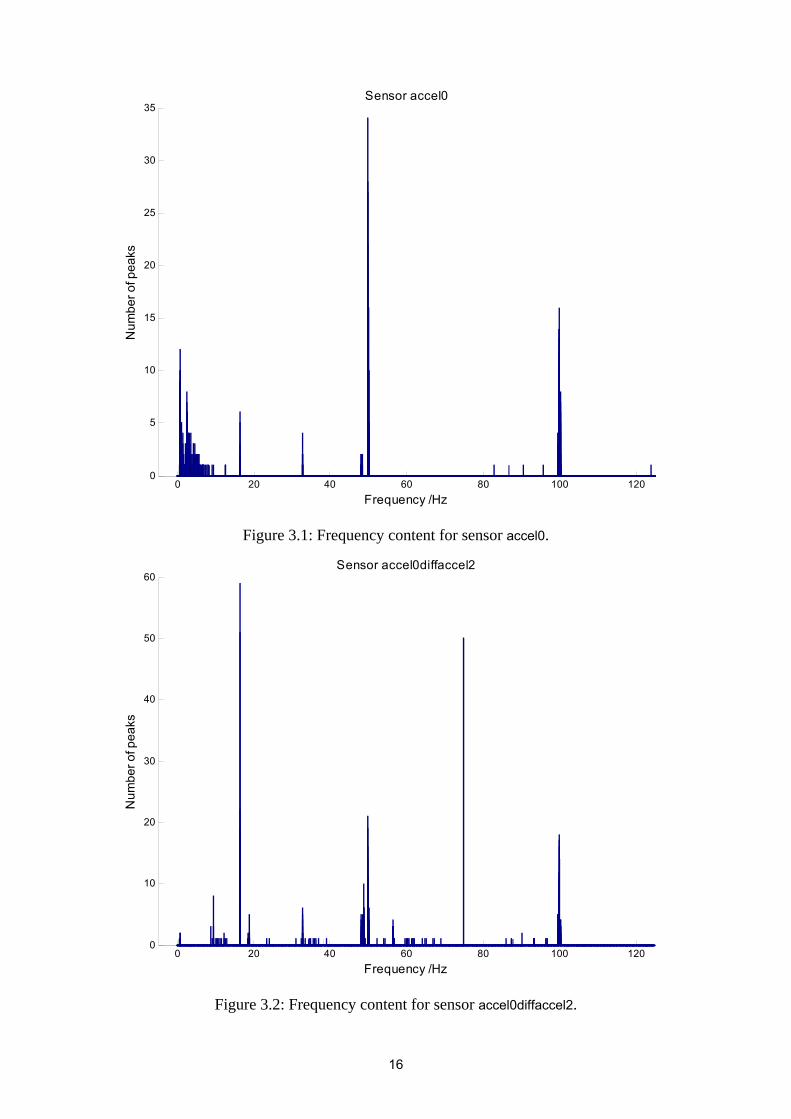
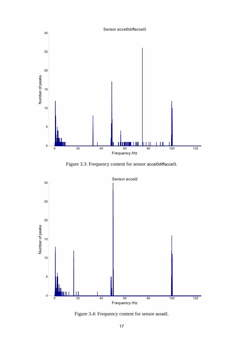
3 Frequency domain analysis
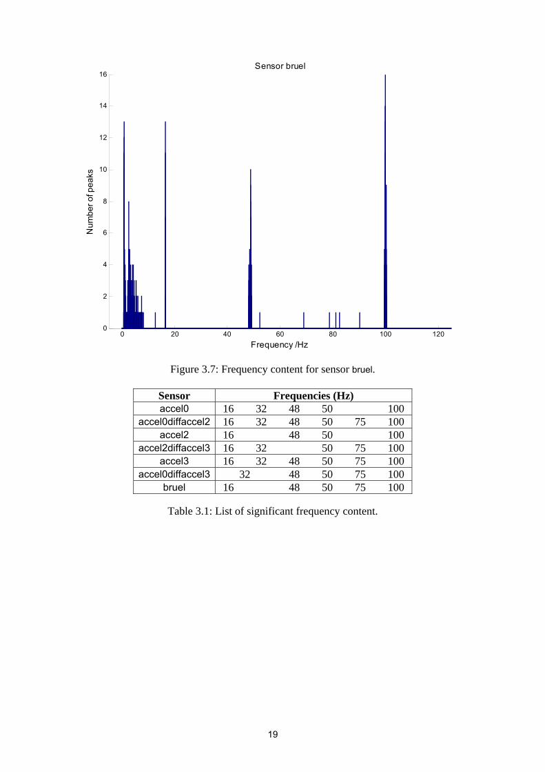
For each sensor, a simple frequency domain analysis method is used to explore all the datasets and try to identify the underlying frequency content of the signals. The spectral density of a signal is calculated over a range of frequencies and those frequencies at which peaks in the spectral density occur are identified and recorded. Using the complete set of frequencies returned for all sensors, a histogram can be plotted to provide a view of the distribution of significant frequency information. Figures 3.1 to 3.7 show, for each sensor, the results of the frequency domain analysis using 8193 frequency values evenly spaced between 0 Hz and 125 Hz (i.e., a frequency interval of 0.01526 Hz). Table 3.1 summarises the main frequencies identified by the frequency domain analysis. Most of the sensors identify 16 Hz, 32 Hz and 48 Hz components. For all of the sensors there are considerable 50 Hz and 100 Hz contributions, possibly indicating mains pick up in the environment. While frequency domain analysis is not a tool that can be used for the explicit identification of non-stationary signals, it can be used to help understand the frequency distribution in the different sensors, and the stability of these signals. It can also help to better estimate the level of “background noise” within the signals, enabling a statistical model of the noise to be developed that can be used for wavelet denoising.
0 20 40 60 80 100 1200
5
10
15
20
25
30
35
Frequency /Hz
Num
ber o
f pea
ks
Sensor accel0
Figure 3.1: Frequency content for sensor accel0.
0 20 40 60 80 100 1200
10
20
30
40
50
60
Frequency /Hz
Num
ber o
f pea
ks
Sensor accel0diffaccel2
Figure 3.2: Frequency content for sensor accel0diffaccel2.
16
0 20 40 60 80 100 1200
5
10
15
20
25
30
Frequency /Hz
Num
ber o
f pea
ks
Sensor accel0diffaccel3
Figure 3.3: Frequency content for sensor accel0diffaccel3.
0 20 40 60 80 100 1200
5
10
15
20
25
30
Frequency /Hz
Num
ber o
f pea
ks
Sensor accel2
Figure 3.4: Frequency content for sensor accel2.
17
0 20 40 60 80 100 1200
2
4
6
8
10
12
14
16
Frequency /Hz
Num
ber o
f pea
ks
Sensor accel2diffaccel3
Figure 3.5: Frequency content for sensor accel2diffaccel3.
0 20 40 60 80 100 1200
5
10
15
20
25
30
35
40
Frequency /Hz
Num
ber o
f pea
ks
Sensor accel3
Figure 3.6: Frequency content for sensor accel3.
18
0 20 40 60 80 100 1200
2
4
6
8
10
12
14
16
Frequency /Hz
Num
ber o
f pea
ks
Sensor bruel
Figure 3.7: Frequency content for sensor bruel.
Sensor Frequencies (Hz) accel0 16 32 48 50 100
accel0diffaccel2 16 32 48 50 75 100 accel2 16 48 50 100
accel2diffaccel3 16 32 50 75 100 accel3 16 32 48 50 75 100
accel0diffaccel3 32 48 50 75 100 bruel 16 48 50 75 100
Table 3.1: List of significant frequency content.
19
4 Wavelet analysis
A transient signal (i.e., a signal containing transient events) is identified by:
1. Abrupt changes in amplitudes, phases or frequencies.
2. Rapid decays in amplitudes.
3. Fast transitions in frequencies and amplitudes.
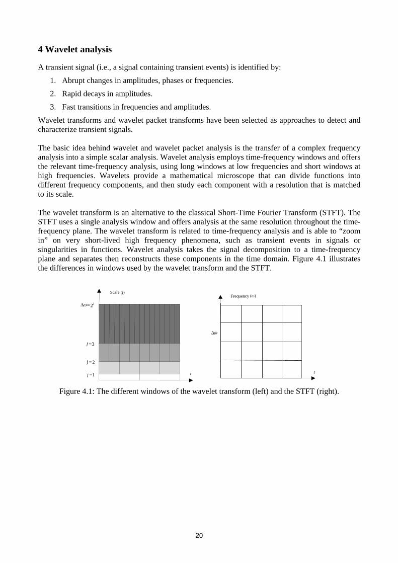
Wavelet transforms and wavelet packet transforms have been selected as approaches to detect and characterize transient signals. The basic idea behind wavelet and wavelet packet analysis is the transfer of a complex frequency analysis into a simple scalar analysis. Wavelet analysis employs time-frequency windows and offers the relevant time-frequency analysis, using long windows at low frequencies and short windows at high frequencies. Wavelets provide a mathematical microscope that can divide functions into different frequency components, and then study each component with a resolution that is matched to its scale. The wavelet transform is an alternative to the classical Short-Time Fourier Transform (STFT). The STFT uses a single analysis window and offers analysis at the same resolution throughout the time-frequency plane. The wavelet transform is related to time-frequency analysis and is able to “zoom in” on very short-lived high frequency phenomena, such as transient events in signals or singularities in functions. Wavelet analysis takes the signal decomposition to a time-frequency plane and separates then reconstructs these components in the time domain. Figure 4.1 illustrates the differences in windows used by the wavelet transform and the STFT.
ω∆
t
Frequency (ω)
j2=∆ω
3=j
2=j
1=j t
Scale (j)
Figure 4.1: The different windows of the wavelet transform (left) and the STFT (right).
20
The following primary properties of the wavelet transform make its use attractive in signal processing:
1. Locality – each wavelet coefficient represents local signal content in space and frequency.
2. Multiresolution – the wavelet transform represents the signal at a nested set of scales.
3. Energy compaction – the wavelet transforms tend to be sparse, i.e., many of the coefficients of the wavelet transform are zero or close to zero.
4. Edge detection – wavelets act as local edge detectors.
Wavelet analysis considered in this report will include:
1. Detection of potential datasets containing transients.
2. Wavelet reconstruction of the transient signals.
3. Wavelet denoising for the identification of transients.
4.1 Use of the discrete wavelet transform to identify datasets potentially containing transient events
In section 2, the use of short-time analysis to identify datasets potentially containing transient events was described. In this section we employ wavelet analysis for the same purpose.
qP
The root mean square deviation and the peak to valley height for the ith dataset on the jth level (scale) are defined as
),( jiPq ),( jiPt
,1),(1
2,,∑
==
m
kkjiq w
mjiP
),(min)(max),( ,,,, kjikkjikt wwjiP −=
where is the wavelet coefficient of the ith dataset on the jth wavelet decomposition level corresponding to the kth translation and is the length of the coefficients vector.
kjiw ,,
m
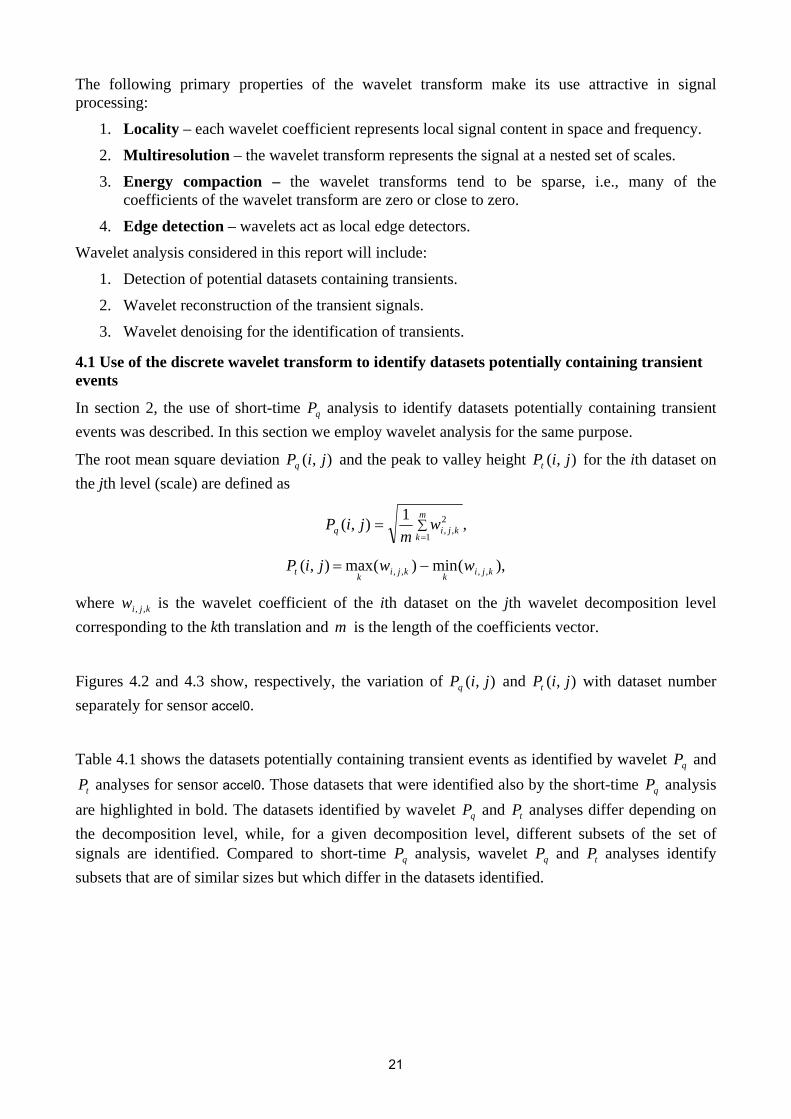
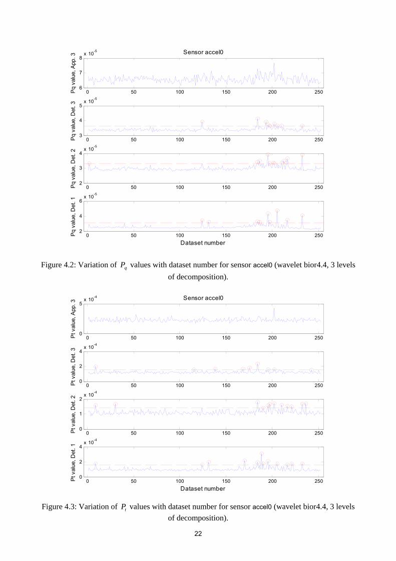
Figures 4.2 and 4.3 show, respectively, the variation of and with dataset number separately for sensor accel0.
),( jiPq ),( jiPt
Table 4.1 shows the datasets potentially containing transient events as identified by wavelet and analyses for sensor accel0. Those datasets that were identified also by the short-time analysis
are highlighted in bold. The datasets identified by wavelet and analyses differ depending on the decomposition level, while, for a given decomposition level, different subsets of the set of signals are identified. Compared to short-time analysis, wavelet and analyses identify subsets that are of similar sizes but which differ in the datasets identified.
qP
tP qP
qP tP
qP qP tP
21
0 50 100 150 200 2506
7
8x 10⁻⁵
Pq
valu
e, A
pp. 3
Sensor accel0
0 50 100 150 200 2503
4
5x 10⁻⁵
Pq
valu
e, D
et. 3
0 50 100 150 200 2502
3
4x 10⁻⁵
Pq v
alue
, Det
. 2
0 50 100 150 200 2502
4
6x 10⁻⁵
Pq v
alue
, Det
. 1
Dataset number
Figure 4.2: Variation of values with dataset number for sensor accel0 (wavelet bior4.4, 3 levels of decomposition).
qP
0 50 100 150 200 2500
5x 10⁻⁴
Pt v
alue
, App
. 3
Sensor accel0
0 50 100 150 200 2500
2
4x 10⁻⁴
Pt v
alue
, Det
. 3
0 50 100 150 200 2500
1
2x 10⁻⁴
Pt v
alue
, Det
. 2
0 50 100 150 200 2500
2
4x 10⁻⁴
Pt v
alue
, Det
. 1
Dataset number
Figure 4.3: Variation of values with dataset number for sensor accel0 (wavelet bior4.4, 3 levels
of decomposition). tP
22

Datasets potentially containing transient events Detail
level qP analysis tP analysis
1 124, 131, 184, 186, 195, 197, 205, 216, 232
9, 124, 131, 170, 184, 188, 190, 195, 205, 216, 221, 232
2 2, 184, 186, 195, 197, 201, 202, 210, 212, 215, 216, 232
9, 30, 184, 190, 195, 197, 202, 210, 216, 221, 232, 236
3 124, 183, 184, 195, 197, 202, 205, 210, 232
9, 115, 138, 168, 175, 184, 195, 202, 242
Table 4.1: List of accel0 datasets identified by wavelet and analysis (using 3 levels of
decomposition) as potentially containing transient events. qP tP
4.2 Use of wavelet packet analysis in finding the time-frequency location of transient events For further reconstruction of the transient events from the original dataset, the discrete wavelet transform has been used to decompose the original signal into scale-space. The wavelet coefficients at each scale have corresponding time-frequency locality and one can obtain time, amplitude and frequency information for transient events.
From experience, it is known that most of the transient events have significant coefficients in the detail band. However, the wavelet transform only repeats the decomposition in the approximation branch, and does not give enough information for the detail branch. In this section we describe the use of wavelet packet analysis to reconstruct transient events.
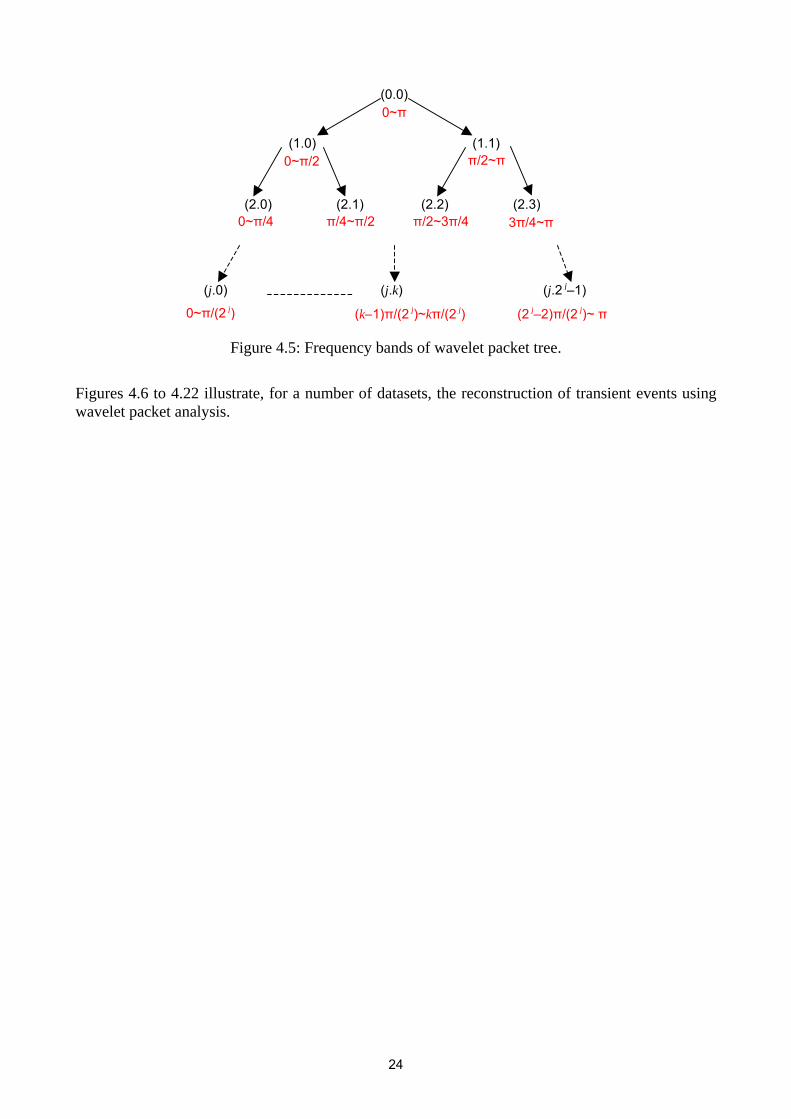
The wavelet packet method is a generalization of wavelet decomposition that offers a richer range of possibilities for signal analysis. In wavelet analysis, a signal is split into an approximation and a detail. The approximation is then itself split into a second-level approximation and detail, and the process is repeated. For an n -level decomposition, there are 1+n possible ways to decompose or encode the signal. In wavelet packet analysis, the details as well as the approximations can be split. This yields different ways to encode the signal. Wavelet packet analysis can obtain much finer information in the detail part than wavelet analysis. Figure 4.4 shows the different decomposition tree structures of wavelet and wavelet packet analysis. Figure 4.5 gives the frequency band of each of the nodes in the wavelet packet analysis tree structure.
n2
Figure 4.4: Tree structures of wavelet decomposition: wavelet analysis (left) and wavelet packet analysis (right).
23
(0.0)
(1.0) (1.1)
(2.0) (2.1) (2.2) (2.3)
(j.0)
(2 j–2)π/(2 j)~ π
(j.2 j–1)
0~π
0~π/2 π/2~π
0~π/4 π/4~π/2 π/2~3π/4 3π/4~π
(k–1)π/(2 j)~kπ/(2 j)
(j.k)
0~π/(2 j)
Figure 4.5: Frequency bands of wavelet packet tree.
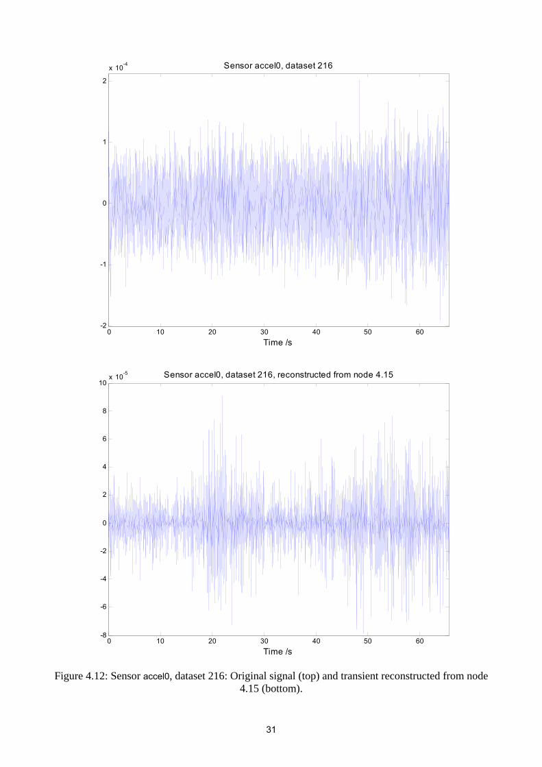
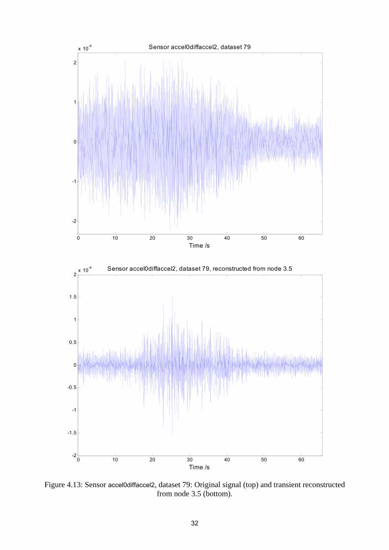
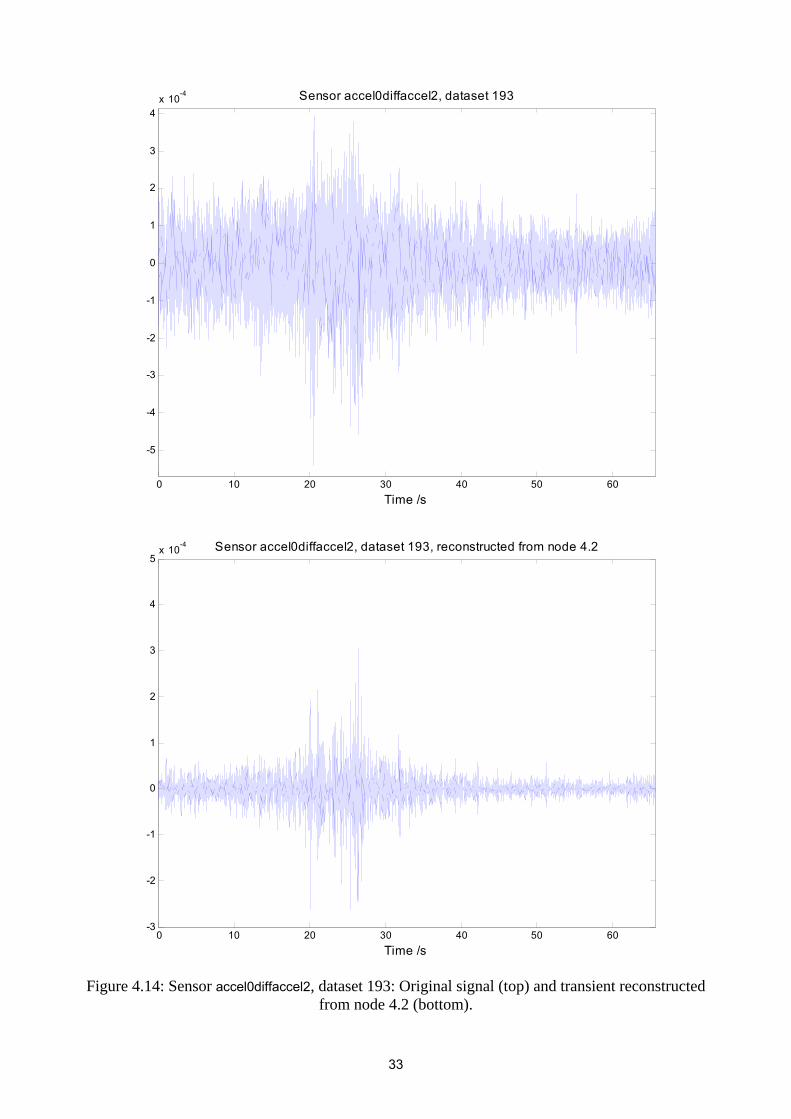
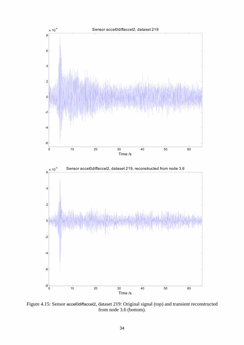
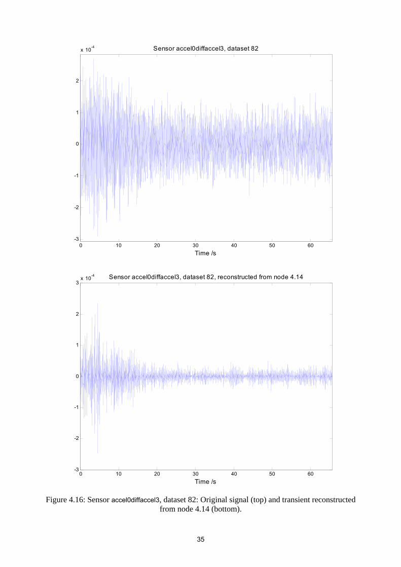
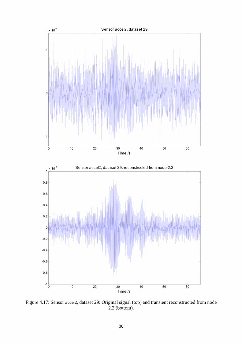
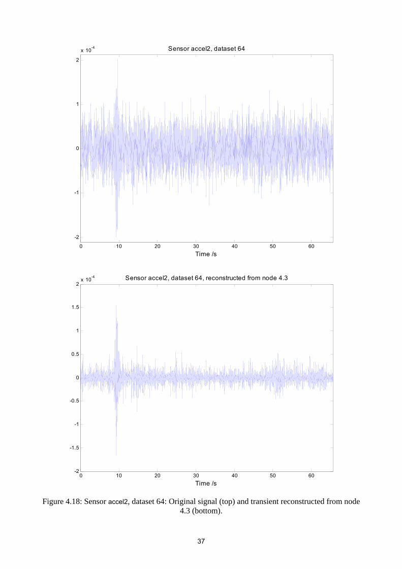
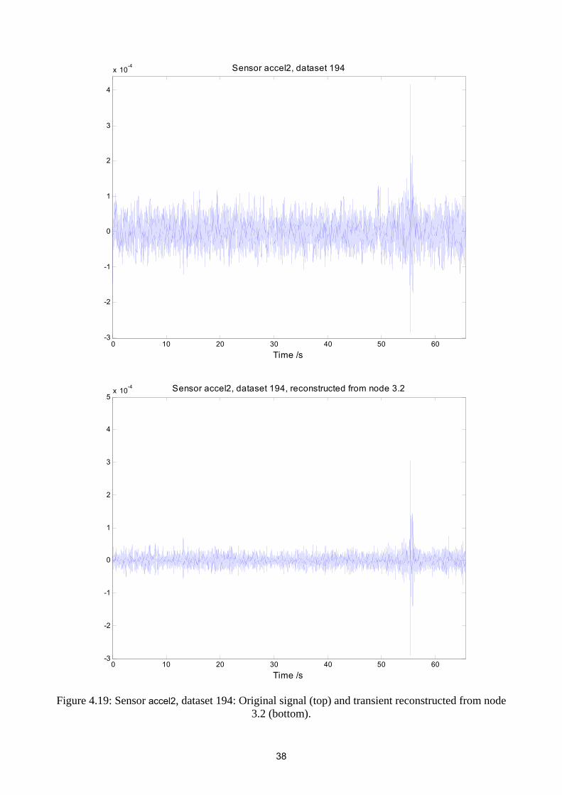
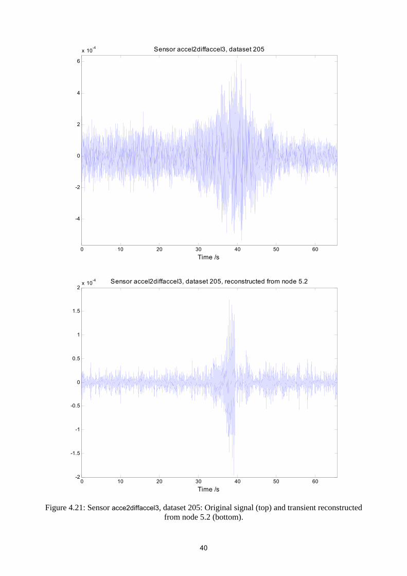
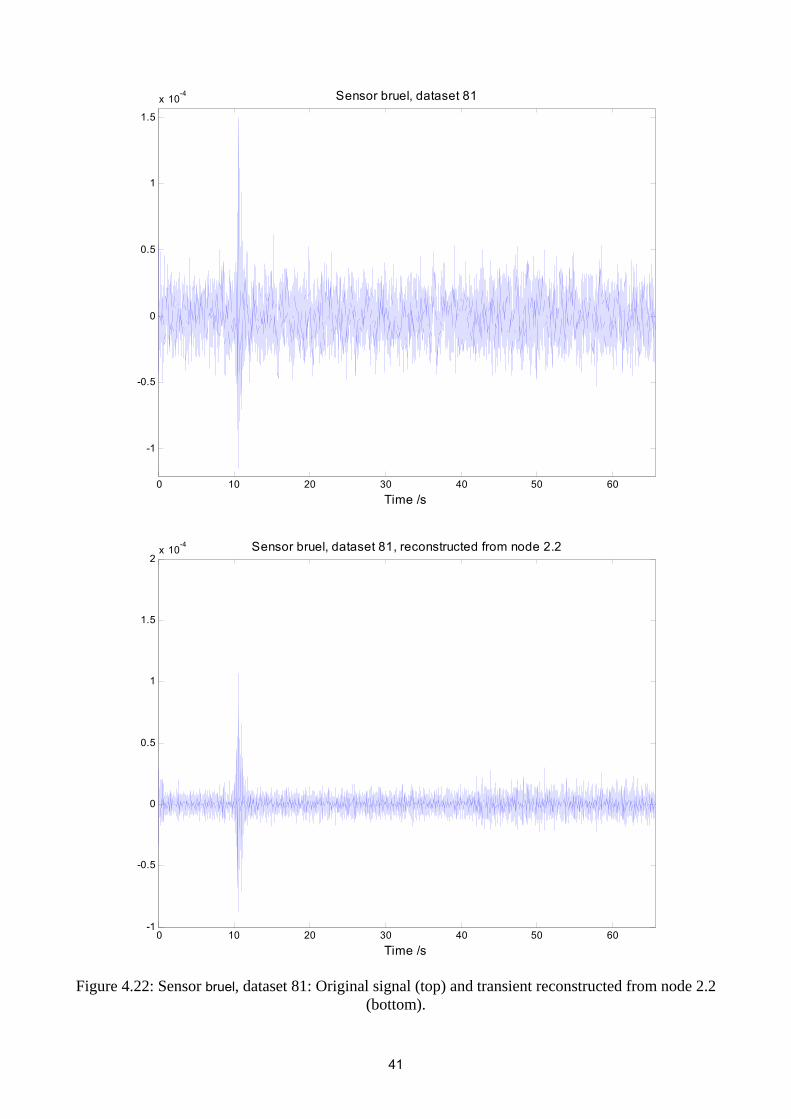
Figures 4.6 to 4.22 illustrate, for a number of datasets, the reconstruction of transient events using wavelet packet analysis.
24
0 10 20 30 40 50 60
-1.5
-1
-0.5
0
0.5
1
1.5
x 10-4
Time /s
Sensor accel0, dataset 40
0 10 20 30 40 50 60-8
-6
-4
-2
0
2
4
6
8x 10
-5
Time /s
Sensor accel0, dataset 40, reconstructed from node 5.28
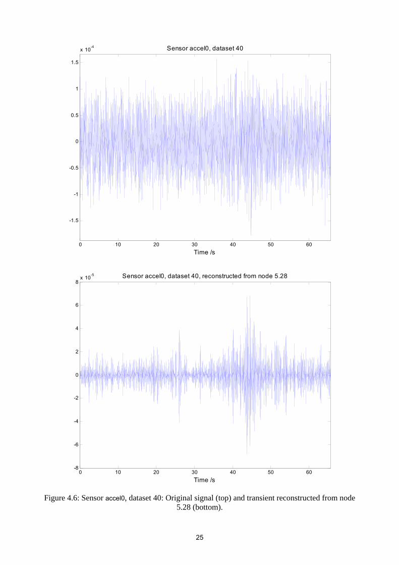
Figure 4.6: Sensor accel0, dataset 40: Original signal (top) and transient reconstructed from node
5.28 (bottom).
25

0 10 20 30 40 50 60
-1.5
-1
-0.5
0
0.5
1
x 10-4
Time /s
Sensor accel0, dataset 71
0 10 20 30 40 50 60-1.5
-1
-0.5
0
0.5
1
1.5x 10
-4
Time /s
Sensor accel0, dataset 71, reconstructed from node 5.2
Figure 4.7: Sensor accel0, dataset 71: Original signal (top) and transient reconstructed from node 5.2
(bottom).
26
0 10 20 30 40 50 60
-2
-1.5
-1
-0.5
0
0.5
1
1.5
x 10-4
Time /s
Sensor accel0, dataset 124
0 10 20 30 40 50 60-1.5
-1
-0.5
0
0.5
1
1.5x 10
-4
Time /s
Sensor accel0, dataset 124, reconstructed from node 3.7
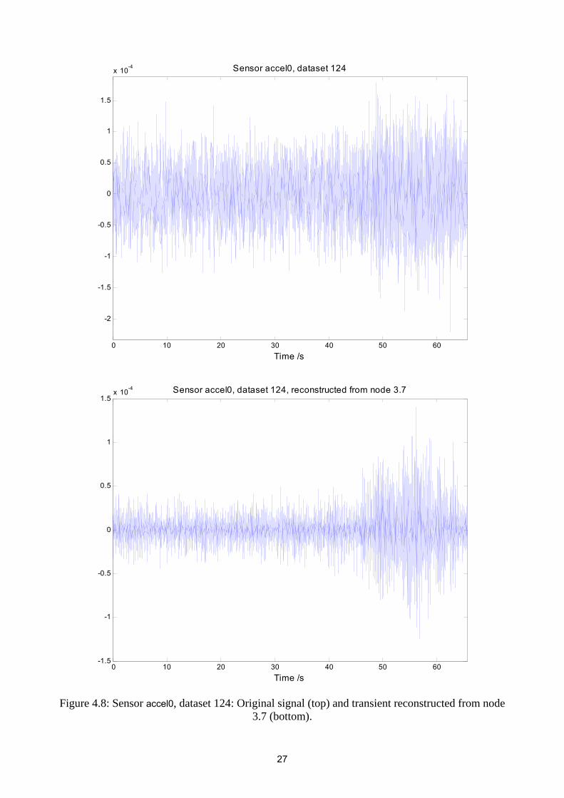
Figure 4.8: Sensor accel0, dataset 124: Original signal (top) and transient reconstructed from node
3.7 (bottom).
27

0 10 20 30 40 50 60
-1.5
-1
-0.5
0
0.5
1
1.5
x 10-4
Time /s
Sensor accel0, dataset 131
0 10 20 30 40 50 60-1.5
-1
-0.5
0
0.5
1
1.5x 10
-4
Time /s
Sensor accel0, dataset 131, reconstructed from node 3.7
Figure 4.9: Sensor accel0, dataset 131: Original signal (top) and transient reconstructed from node
3.7 (bottom).
28

0 10 20 30 40 50 60
-2.5
-2
-1.5
-1
-0.5
0
0.5
1
1.5
2
x 10-4
Time /s
Sensor accel0, dataset 188
0 10 20 30 40 50 60-3
-2
-1
0
1
2
3
4
5x 10
-4
Time /s
Sensor accel0, dataset 188, reconstructed from node 3.7
Figure 4.10: Sensor accel0, dataset 188: Original signal (top) and transient reconstructed from node
3.7 (bottom).
29
0 10 20 30 40 50 60
-1.5
-1
-0.5
0
0.5
1
1.5
2
x 10-4
Time /s
Sensor accel0, dataset 202
0 10 20 30 40 50 60-1.5
-1
-0.5
0
0.5
1
1.5
2
2.5x 10
-4
Time /s
Sensor accel0, dataset 202, reconstructed from node 4.1
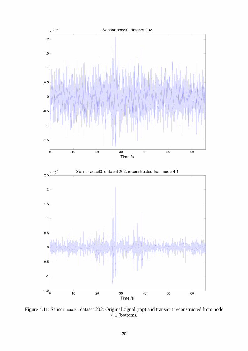
Figure 4.11: Sensor accel0, dataset 202: Original signal (top) and transient reconstructed from node
4.1 (bottom).
30
0 10 20 30 40 50 60-2
-1
0
1
2
x 10-4
Time /s
Sensor accel0, dataset 216
0 10 20 30 40 50 60-8
-6
-4
-2
0
2
4
6
8
10x 10
-5
Time /s
Sensor accel0, dataset 216, reconstructed from node 4.15
Figure 4.12: Sensor accel0, dataset 216: Original signal (top) and transient reconstructed from node
4.15 (bottom).
31
0 10 20 30 40 50 60
-2
-1
0
1
2
x 10-4
Time /s
Sensor accel0diffaccel2, dataset 79
0 10 20 30 40 50 60-2
-1.5
-1
-0.5
0
0.5
1
1.5
2x 10
-4
Time /s
Sensor accel0diffaccel2, dataset 79, reconstructed from node 3.5
Figure 4.13: Sensor accel0diffaccel2, dataset 79: Original signal (top) and transient reconstructed
from node 3.5 (bottom).
32
0 10 20 30 40 50 60
-5
-4
-3
-2
-1
0
1
2
3
4x 10
-4
Time /s
Sensor accel0diffaccel2, dataset 193
0 10 20 30 40 50 60-3
-2
-1
0
1
2
3
4
5x 10
-4
Time /s
Sensor accel0diffaccel2, dataset 193, reconstructed from node 4.2
Figure 4.14: Sensor accel0diffaccel2, dataset 193: Original signal (top) and transient reconstructed
from node 4.2 (bottom).
33
0 10 20 30 40 50 60
-6
-4
-2
0
2
4
6
8x 10
-4
Time /s
Sensor accel0diffaccel2, dataset 219
0 10 20 30 40 50 60-8
-6
-4
-2
0
2
4
6x 10
-4
Time /s
Sensor accel0diffaccel2, dataset 219, reconstructed from node 3.6
Figure 4.15: Sensor accel0diffaccel2, dataset 219: Original signal (top) and transient reconstructed
from node 3.6 (bottom).
34
0 10 20 30 40 50 60-3
-2
-1
0
1
2
x 10-4
Time /s
Sensor accel0diffaccel3, dataset 82
0 10 20 30 40 50 60-3
-2
-1
0
1
2
3x 10
-4
Time /s
Sensor accel0diffaccel3, dataset 82, reconstructed from node 4.14
Figure 4.16: Sensor accel0diffaccel3, dataset 82: Original signal (top) and transient reconstructed
from node 4.14 (bottom).
35
0 10 20 30 40 50 60
-1
0
1
x 10-4
Time /s
Sensor accel2, dataset 29
0 10 20 30 40 50 60-1
-0.8
-0.6
-0.4
-0.2
0
0.2
0.4
0.6
0.8
1x 10
-4
Time /s
Sensor accel2, dataset 29, reconstructed from node 2.2
Figure 4.17: Sensor accel2, dataset 29: Original signal (top) and transient reconstructed from node
2.2 (bottom).
36
0 10 20 30 40 50 60
-2
-1
0
1
2
x 10-4
Time /s
Sensor accel2, dataset 64
0 10 20 30 40 50 60-2
-1.5
-1
-0.5
0
0.5
1
1.5
2x 10
-4
Time /s
Sensor accel2, dataset 64, reconstructed from node 4.3
Figure 4.18: Sensor accel2, dataset 64: Original signal (top) and transient reconstructed from node
4.3 (bottom).
37
0 10 20 30 40 50 60-3
-2
-1
0
1
2
3
4
x 10-4
Time /s
Sensor accel2, dataset 194
0 10 20 30 40 50 60-3
-2
-1
0
1
2
3
4
5x 10
-4
Time /s
Sensor accel2, dataset 194, reconstructed from node 3.2
Figure 4.19: Sensor accel2, dataset 194: Original signal (top) and transient reconstructed from node
3.2 (bottom).
38

0 10 20 30 40 50 60-6
-4
-2
0
2
4
x 10-4
Time /s
Sensor accel2diffaccel3, dataset 189
0 10 20 30 40 50 60-5
-4
-3
-2
-1
0
1
2
3
4
5x 10
-4
Time /s
Sensor accel2diffaccel3, dataset 189, reconstructed from node 3.7
Figure 4.20: Sensor accel2diffaccel3, dataset 189: Original signal (top) and transient reconstructed
from node 3.7 (bottom).
39
0 10 20 30 40 50 60
-4
-2
0
2
4
6
x 10-4
Time /s
Sensor accel2diffaccel3, dataset 205
0 10 20 30 40 50 60-2
-1.5
-1
-0.5
0
0.5
1
1.5
2x 10
-4
Time /s
Sensor accel2diffaccel3, dataset 205, reconstructed from node 5.2
Figure 4.21: Sensor acce2diffaccel3, dataset 205: Original signal (top) and transient reconstructed
from node 5.2 (bottom).
40
0 10 20 30 40 50 60
-1
-0.5
0
0.5
1
1.5
x 10-4
Time /s
Sensor bruel, dataset 81
0 10 20 30 40 50 60-1
-0.5
0
0.5
1
1.5
2x 10
-4
Time /s
Sensor bruel, dataset 81, reconstructed from node 2.2
Figure 4.22: Sensor bruel, dataset 81: Original signal (top) and transient reconstructed from node 2.2
(bottom).
41
One can see from the figures that the wavelet transform can increase the transient to residual ratio significantly, illustrating the use of wavelets in detecting transient signals while keeping their time and frequency local properties.
However there are some problems:
1. If only one or two nodes from the wavelet decomposition tree are used for reconstruction, the transient signals cannot be separated precisely, and they will still include much noise or stationary signal.
2. The transient event propagates through many scales in the wavelet decomposition tree.
3. For different signals, the most significant transient to residual ratios are not at the same level and finding the level automatically is therefore not easy. Further work includes developing a statistical model of the signal and identifying the dependence between wavelet coefficients at different levels.
In the following section the use of wavelet denoising and statistical modelling to overcome these problems is described.
4.3 Wavelet denoising The detection of transient events can also be thought of as a denoising problem. The measured signal is modelled as z
,nsz +=
where is the true signal (or the non-stationary signal, transient events) and n is the noise (or the stationary signals). The aim of denoising is to estimate as accurately as possible from .
ss z
In the wavelet domain, if the dependency of wavelet coefficients among different levels is neglected, the problem can be formulated as
inisiz www ,,, += ,
where i is the wavelet level, is the noisy wavelet coefficient, is the true coefficient and represents noise.
izw , isw ,
inw ,
The denoising problem is to estimate coefficients as accurately as possible from and then reconstruct the signal.
isw , izw ,
4.3.1 Soft and hard thresholding in the wavelet domain
Simple denoising algorithms that use the wavelet transform consist of three steps:
1. Calculate the wavelet transform of the (noisy) signal.
2. Modify the noisy wavelet coefficients according to some rules.
3. Calculate the inverse wavelet transform using the modified coefficients to reconstruct the denoised signal.
One of the well-known rules for the second step is thresholding analysis of which there are two forms: soft and hard thresholding.
The main idea of soft thresholding is to subtract a threshold value T from all coefficients larger than T and to set all other coefficients to zero, i.e.,
⎪⎩
⎪⎨
⎧
−<+>−
≤
=.if
,if,if0
ˆTwTw
TwTwTw
w
zz
zz
z
s
42
In hard thresholding all coefficients smaller than T are set to zero while the values of all other coefficients are unchanged, i.e.,
⎩⎨⎧
>
≤=
.if,if0
ˆTwwTw
wzz
zs
The selection of the threshold value T is the key issue in denoising. The simplest choice is to use the variance of the wavelet coefficients on each level as the threshold value. In the following section, the maximum a posteriori (MAP) estimator is used to obtain the threshold value.
4.3.2 Marginal model for wavelet denoising From MAP, estimates of the true wavelet coefficients can be obtained using:
).(maxarg)(ˆ zswww
zs wwpwwzs
s
=
Using Bayes rules one gets:
[ ][ ][ ].)()(maxarg
)()(maxarg
)()(maxarg)(ˆ
swnww
swszww
swszwww
zs
wpwp
wpwwp
wpwwpww
sns
sns
sszs
⋅=
⋅−=
⋅=
These equations allow us to write this estimation in terms of the probability density function (PDF) of the noise and the PDF of the signal coefficient.
Assume the PDF of the noise is zero mean Gaussian function with variance : 2nσ
,2
exp2
1)(2
2
⎟⎟⎠
⎞⎜⎜⎝
⎛−⋅=
n
n
nnw
wwp
n σπσ
and assume the wavelet coefficients of the true signal have PDF
.2
exp2
1)( ⎟⎟⎠
⎞⎜⎜⎝
⎛−⋅=
s
s
ssw
wwp
s σσ
One obtains
⎪⎪⎪
⎩
⎪⎪⎪
⎨
⎧
−<+
>
≤
=
.2 if 2
,2 if 2-
,2 if 0
ˆ
22
22
2
s
nz
s
nz
s
nz
s
nz
s
nz
s
ww
ww
w
w
σσ
σσ
σσ
σσ
σσ
This is a soft thresholding method, where the threshold value is s
nTσσ 22
= .
The noise variance nσ can be estimated from the empirical model, and the variance of true signal can be estimated from:
22 ˆˆ nzs σσσ −= ,
where zσ can be estimated by its neighbour: ∑∈
=M
kwNiwzz
zz
iwM ))(()(
22 )(1σ̂ .
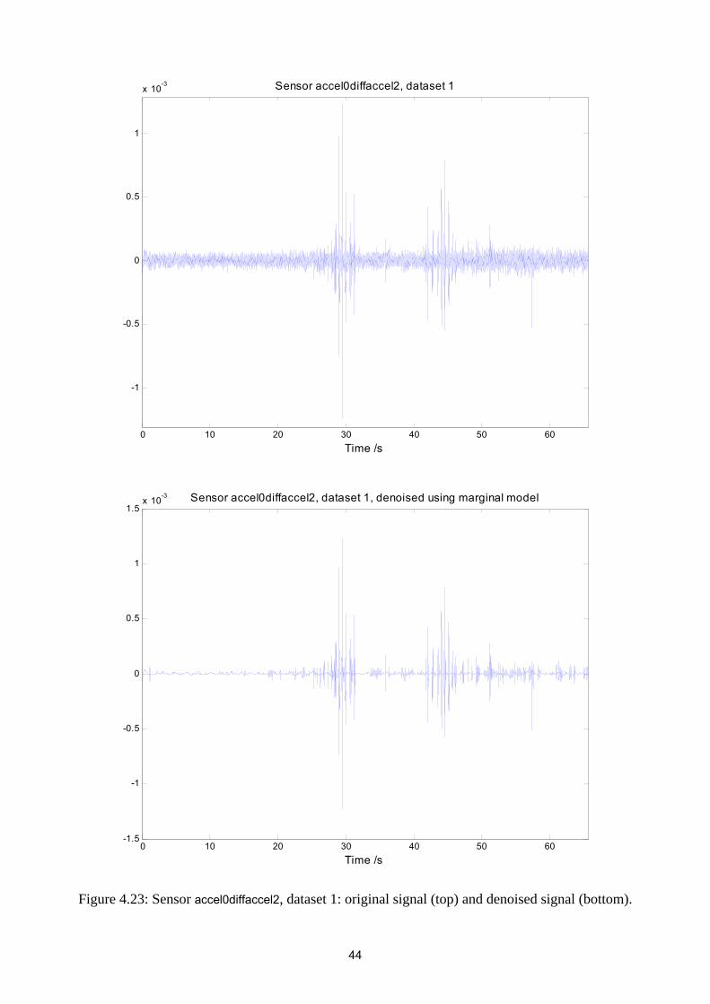
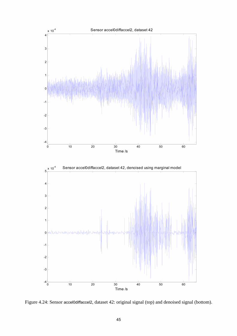
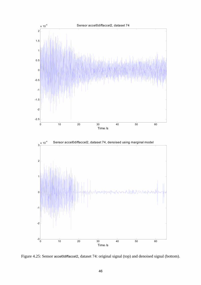
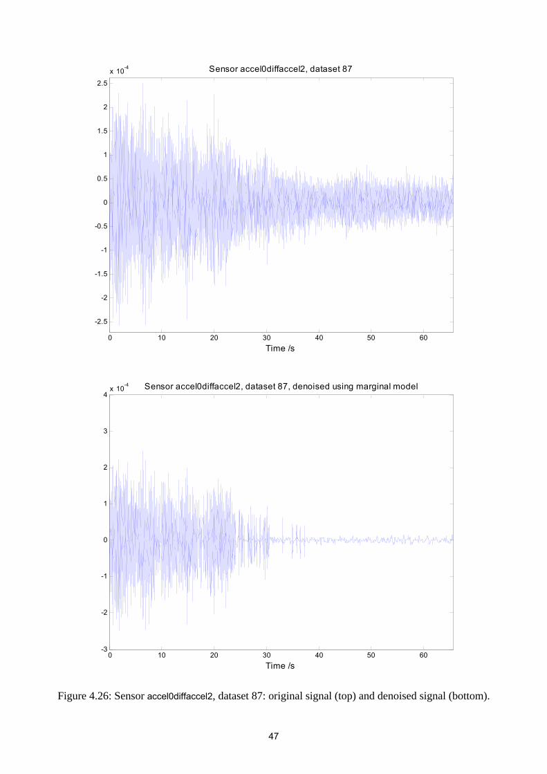
Figures 4.23 to 4.27 show results obtained using the marginal model method described above. 43
0 10 20 30 40 50 60
-1
-0.5
0
0.5
1
x 10-3
Time /s
Sensor accel0diffaccel2, dataset 1
0 10 20 30 40 50 60-1.5
-1
-0.5
0
0.5
1
1.5x 10
-3
Time /s
Sensor accel0diffaccel2, dataset 1, denoised using marginal model
Figure 4.23: Sensor accel0diffaccel2, dataset 1: original signal (top) and denoised signal (bottom).
44
0 10 20 30 40 50 60-4
-3
-2
-1
0
1
2
3
4x 10
-4
Time /s
Sensor accel0diffaccel2, dataset 42
0 10 20 30 40 50 60-4
-3
-2
-1
0
1
2
3
4
5x 10
-4
Time /s
Sensor accel0diffaccel2, dataset 42, denoised using marginal model
Figure 4.24: Sensor accel0diffaccel2, dataset 42: original signal (top) and denoised signal (bottom).
45
0 10 20 30 40 50 60
-2.5
-2
-1.5
-1
-0.5
0
0.5
1
1.5
2
x 10-4
Time /s
Sensor accel0diffaccel2, dataset 74
0 10 20 30 40 50 60-3
-2
-1
0
1
2
3x 10
-4
Time /s
Sensor accel0diffaccel2, dataset 74, denoised using marginal model
Figure 4.25: Sensor accel0diffaccel2, dataset 74: original signal (top) and denoised signal (bottom).
46
0 10 20 30 40 50 60
-2.5
-2
-1.5
-1
-0.5
0
0.5
1
1.5
2
2.5
x 10-4
Time /s
Sensor accel0diffaccel2, dataset 87
0 10 20 30 40 50 60-3
-2
-1
0
1
2
3
4x 10
-4
Time /s
Sensor accel0diffaccel2, dataset 87, denoised using marginal model
Figure 4.26: Sensor accel0diffaccel2, dataset 87: original signal (top) and denoised signal (bottom).
47
0 10 20 30 40 50 60
-6
-4
-2
0
2
4
6
8x 10
-4
Time /s
Sensor accel0diffaccel2, dataset 219
0 10 20 30 40 50 60-8
-6
-4
-2
0
2
4
6
8
10x 10
-4
Time /s
Sensor accel0diffaccel2, dataset 219, denoised using marginal model
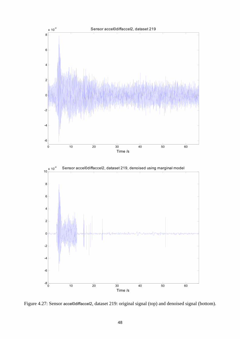
Figure 4.27: Sensor accel0diffaccel2, dataset 219: original signal (top) and denoised signal (bottom).
48
If the MAP estimator is used, a priori knowledge about the distribution of wavelet coefficients is required leading to the problem of deciding on the distribution that represents the wavelet coefficients. This problem can be overcome using empirical histogram analysis, which requires a large amount of data to find the most likely statistical model to match the wavelet coefficients.
In this section we have introduced the wavelet transform for denoising (transient events detection) dependent on the marginal model. In the marginal model, we do not consider the dependency relation among the wavelet coefficients.
In section 4.2, we only use one of the most significant levels to reconstruct the transient event; it has lost much information about the transient events that appear at other scales. Bivariate models can be used to find the dependency of the coefficients of the transient events at different levels.
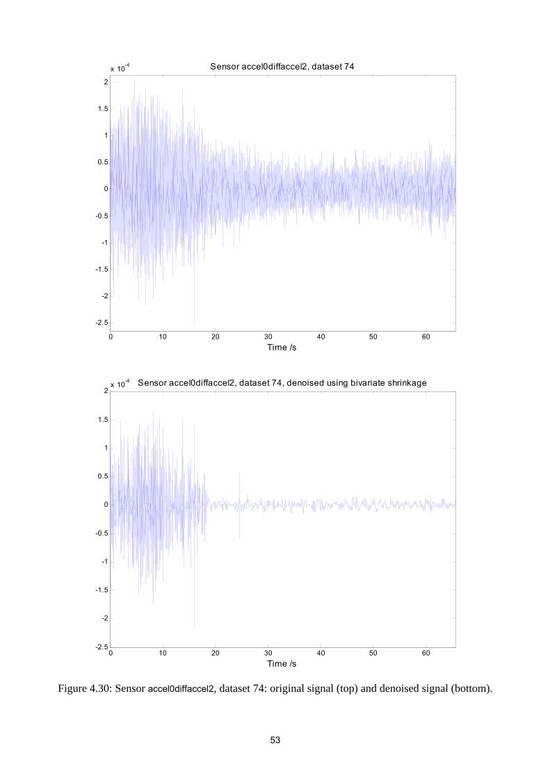
4.3.3 Bivariate shrinkage Marginal models cannot model the statistical dependencies between wavelet coefficients. However, there are strong dependencies between neighbouring coefficients, e.g., between a coefficient, its parent (adjacent coarser scale locations), and their siblings (adjacent spatial locations). Levent Sendur and Ivan Selesnick have proposed a jointly non-Gaussian model to characterize the dependency between a coefficient and its parent and to derive the corresponding bivariate MAP estimators based on noisy wavelet coefficients in detail. This model is used in this section.
Let represent the wavelet coefficient of parent of ( is the wavelet coefficient at the
same position as the child wavelet coefficient ), then pSw
cSwpSw
cSw
,ccc nSZ www +=
,PPP nSZ www +=
where and are noisy observations of and respectively, and and represent noise.
cZwpZw
cSw ,pSw
cnwpnw
We can write
,nsz www +=
where , and ),(pc zzz www = ),(
pc sss www = ),(pc nnn www = .
From the MAP estimator
[ ][ ][ ].)()(maxarg
)()(maxarg
)()(maxarg
)(maxarg)(ˆ
swnww
swszww
swszwww
zswww
zs
wpwp
wpwwp
wpwwp
wwpww
sns
sns
sszs
zss
⋅=
⋅−=
⋅=
=
From the empirical histogram, Levent Sendur has recommended the joint PDF of the noise and true signal to be
,2
exp2
1)( 2
22
21
2 ⎟⎟⎠
⎞⎜⎜⎝
⎛ +=
nnnw
nnwP
n σπσ
49
.3exp2
3)( 222 ⎟⎟
⎠
⎞⎜⎜⎝
⎛+−=
cps sssw wwwPσπσ
By using the maximum likelihood method, the MAP estimator can be written as
,
3
ˆ22
222
c
pc
pc
c z
zz
nzz
s www
ww
w ⋅+
⎟⎟⎠
⎞⎜⎜⎝
⎛−+
= +σσ
where is defined as +)(g
⎩⎨⎧ >
=+ .otherwise,0if0
)(g
gg
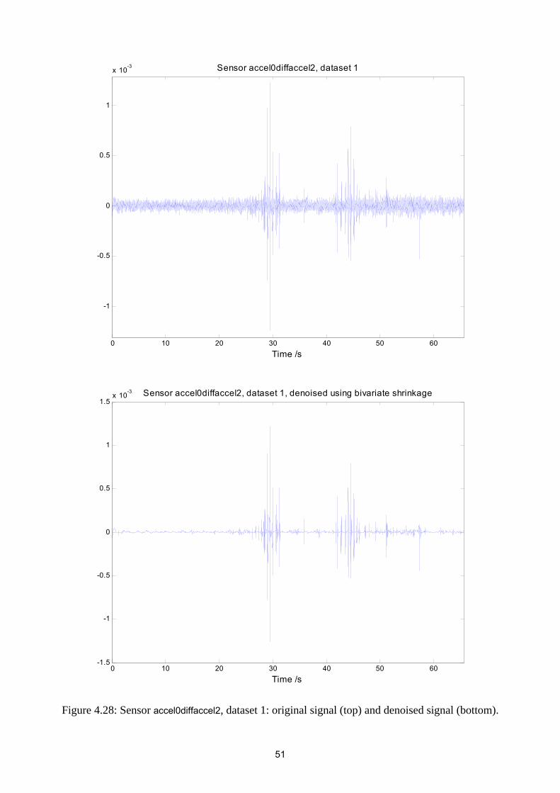
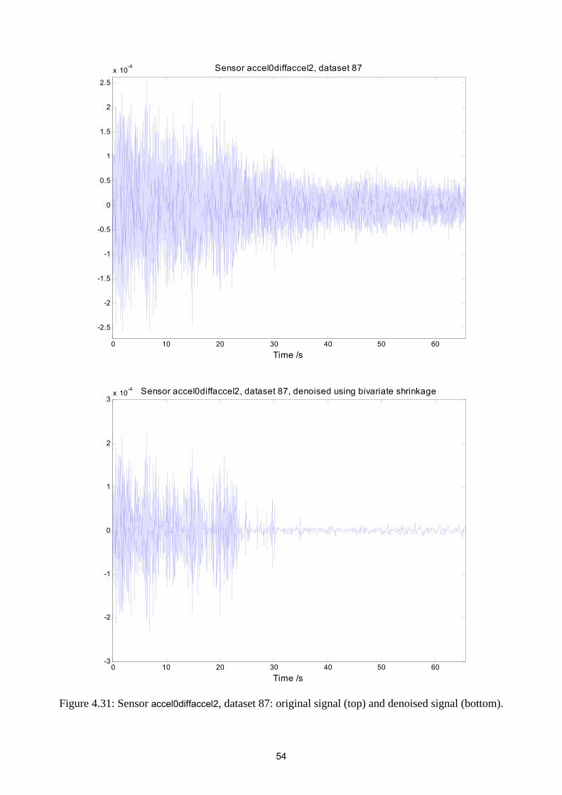
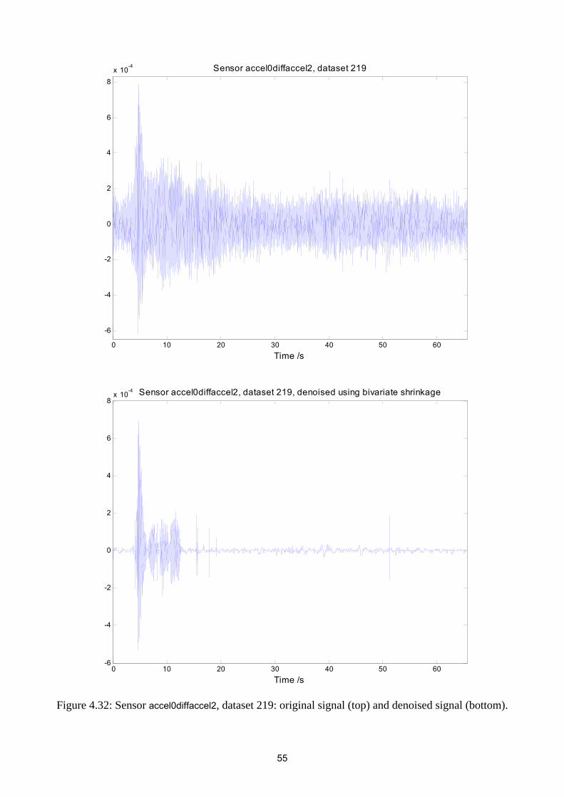
Figures 4.28 to 4.32 show results obtained using bivariate shrinkage.
50
0 10 20 30 40 50 60
-1
-0.5
0
0.5
1
x 10-3
Time /s
Sensor accel0diffaccel2, dataset 1
0 10 20 30 40 50 60-1.5
-1
-0.5
0
0.5
1
1.5x 10
-3
Time /s
Sensor accel0diffaccel2, dataset 1, denoised using bivariate shrinkage
Figure 4.28: Sensor accel0diffaccel2, dataset 1: original signal (top) and denoised signal (bottom).
51

0 10 20 30 40 50 60-4
-3
-2
-1
0
1
2
3
4x 10
-4
Time /s
Sensor accel0diffaccel2, dataset 42
0 10 20 30 40 50 60-4
-3
-2
-1
0
1
2
3
4x 10
-4
Time /s
Sensor accel0diffaccel2, dataset 42, denoised using bivariate shrinkage
Figure 4.29: Sensor accel0diffaccel2, dataset 42: original signal (top) and denoised signal (bottom).
52
0 10 20 30 40 50 60
-2.5
-2
-1.5
-1
-0.5
0
0.5
1
1.5
2
x 10-4
Time /s
Sensor accel0diffaccel2, dataset 74
0 10 20 30 40 50 60-2.5
-2
-1.5
-1
-0.5
0
0.5
1
1.5
2x 10
-4
Time /s
Sensor accel0diffaccel2, dataset 74, denoised using bivariate shrinkage
Figure 4.30: Sensor accel0diffaccel2, dataset 74: original signal (top) and denoised signal (bottom).
53
0 10 20 30 40 50 60
-2.5
-2
-1.5
-1
-0.5
0
0.5
1
1.5
2
2.5
x 10-4
Time /s
Sensor accel0diffaccel2, dataset 87
0 10 20 30 40 50 60-3
-2
-1
0
1
2
3x 10
-4
Time /s
Sensor accel0diffaccel2, dataset 87, denoised using bivariate shrinkage
Figure 4.31: Sensor accel0diffaccel2, dataset 87: original signal (top) and denoised signal (bottom).
54
0 10 20 30 40 50 60
-6
-4
-2
0
2
4
6
8x 10
-4
Time /s
Sensor accel0diffaccel2, dataset 219
0 10 20 30 40 50 60-6
-4
-2
0
2
4
6
8x 10
-4
Time /s
Sensor accel0diffaccel2, dataset 219, denoised using bivariate shrinkage
Figure 4.32: Sensor accel0diffaccel2, dataset 219: original signal (top) and denoised signal (bottom).
55
56
5 Conclusions
Detection of transient events embedded in noise is a problem of great interest in several applications. In this report, three tools have been used to analyse signals containing transient events: time domain analysis, frequency histogram analysis, and wavelet analysis.
Based on the assumption that the transient events are followed by an abrupt change in amplitude, short-time root-mean-square analysis has been successfully used to identify datasets that potentially contain transient events, significantly reducing the workload required to analyse all the data sets.
Frequency analysis is not a tool for the identification of non-stationary signals. However, it has been used to help to understand the frequency structure of signals, frequency distribution in the different sensors, and the stability of these signal. The result can also help us to understand and build the “background noise” of the stationary signal, which can be used to find the empirical statistics of the stationary signal, and can be used for the wavelet denoising method that is based on the statistical model of the noise.
Wavelet analysis focuses mainly on wavelet domain denoising. Two wavelet domain denoising methods, the marginal model and the bivariate model, have been successfully used to extract transient events. In the marginal model, dependencies among the wavelet coefficients are not considered whereas the bivariate model considers the dependencies of coefficients at different levels. The bivariate model requires a priori knowledge of the statistics of the wavelet coefficients.
57
References
I. Daubechies, Ten lectures on wavelets, 1st edn, Philadelphia, PA:SIAM. C. K. Chui, An introduction on wavelets. Philadelphia, PA: SIAM. S. Mallat, A theory for multiresolution signal decomposition: the wavelet representation, IEEE Trans. Pattern Analysis Machine Intelligence, 11 (674-693) 1989. S. Mallat, Characterization of signals form multiscale edges, IEEE Transactions on Pattern Analysis and Machines Intelligence, 14 (710-732), 1992. S. Mallat, Singularity detection and processing with wavelets, IEEE Trans. Inform. Theory, 38 (617-643). Y. Meyer, Wavelets: algorithms and applications, 1st edn. Philadelphia, PA: SIAM, 1993. D. L. Donoho, Denoising by Soft Thresholding, IEEE Trans. Inform. Theory, 41 (613-627), 1995. D. L. Donoho, I. Johnstone, Adapting to unknown smoothness via wavelet shrinkage, J. Amer. Stat. Assoc., 99 (1200-1224), 1995. Levent Sendur, Ivan W. Selesnick, Bivariate Shrinkage with Local Variance Estimation, IEEE Signal Processing Letters, 9 (438-441), 2002. Levent Sendur, Ivan W. Selesnick, Bivariate Shirinkage Functions for Wavelet-based Denoising Exploiting Interscale Dependency, IEEE Tranctions on signal Processing, 50 (2744-2756), 2002. Matthew Crouse, Robert Nowak, Richard Baraniuk, Wavelet-based Statistical Signal Processing Using Hidden Markov Models, IEEE Transactions On Signal Processing, 16 (886-902), 1998. Justin K. Romberg, Hyeokho Choi, Richad G. Baraniuk, Bayesian Tree-Structured Image Modeling using Wavelet-domain Hidden Markov Models, IEEE Transactions On Signal Processing, 10 (1056-1068), 2001. N. Kingsbury, Image processing with complex wavelets, Phil. Tran. R. Soc. Lond. A, 357 (2543-2560), 1999. N. Kingsbury, Complex Wavelets for Shift Invariant Analysis and Filtering of Signals. J. Appli. Comput. Harmonic Anal. 10 (234-253), 2001. G. J. Lord, E. Pardo-Iquzquiza, I. M. Smith, A Practical Guide to Wavelets for Metrology, NPL report, 2000. Javier Portilla, Vasily Strela, Martin J. Wainwright, Eero P. Simoncelli, Image Denoising Using Scale Mixtures of Gaussians in the Wavelet Domain, IEEE Transactions on Image Processing, 12 (1338-1351), 2003. Michel Misitim,Yves Misiti, Georges Oppenheim, Jean-Michel Poggi, Wavelet Toolbox for Use with Matlab. Rice University, http://www.dsp.ece.rice.edu/.
58
University of Cambridge, http://www-sigproc.eng.cam.ac.uk/~ngk/. Polytechnic University, New York, http://taco.poly.edu/WaveletSoftware/index.html. The Wavelet Digest, http://www.wavelet.org/. The MathWorks Wavelet Toolbox, http://www.mathworks.com/access/helpdesk/help/toolbox/wavelet/wavelet.shtml