transient simulation technique for hvdc systems simulation technique for hvdc systems ... ensure...
TRANSCRIPT
Transient Simulation Technique for HVDC Systems
Yongnam Cho, Student Member, IEEE, George J. Cokkinides, Senior Member, IEEE, and
A.P. Meliopoulos, Fellow, IEEE
Abstract--This paper presents an advanced transient
simulation method, the quadratic integration method, and its
application to the simulation of HVDC systems. The quadratic
integration method demonstrates several superior features that
ensure higher fidelity and stability in transient analysis of
systems with nonlinearities and switching subsystems: nonlinear
model equations are converted into a set of linear and quadratic
equation with the introduction of new variables (model
quadratization) and the resulting equations are integrated
assuming a quadratic variation over the integration time step
(quadratic integration). The method eliminates fictitious
oscillations exhibited by trapezoidal integration. Furthermore,
the quadratic integration method is more accurate and robust
than trapezoidal integration and other transient analysis tools.
In this paper, the superior properties of the quadratic
integration in power system transient analysis are demonstrated
by comparing the quadratic integration with the trapezoidal
integration in the simulation of High Voltage Direct Current
(HVDC) system with switching subsystems and nonlinear
components.
Keywords: Quadratic integration, numerical method, transient
simulation, numerical oscillation, 12-pulse converter, equidistant
control, nonlinear transformer.
I. INTRODUCTION
INCE the demands for utilizing long distant sources, and
linking different frequency systems have been increasing,
HVDC transmission systems, are becoming one of the most
promising technologies to meet the need for reliable and cost
effective transmission. Specially, the rapid increase of wind
power in remote locations has accelerated the necessity of
more advanced, reliable and cost effective applications of
HVDC transmission systems. High fidelity transient
simulation technique can be a useful tool for the advanced
design and optimization of HVDC transmission systems with
nonlinearities and switching subsystems.
Numerical integration methods have been extensively
studied and applied to transient analysis of power systems
with nonlinear and switching components. The most
predominant method among the time domain transient
simulation methods is trapezoidal integration due to its
property of absolute stability (A-stable) [1],[2]. However, the
trapezoidal integration is problematic when applied to network
systems with nonlinearities and switching subsystems.
Fictitious oscillations can be generated, when the state of the
Yongnam Cho, George J. Cokkinides, A.P Meliopoulos are with the School of
Electrical and Computer Engineering , Georgia Institute of Technology,
Atlanta, GA,30332 USA (e-mail: [email protected], [email protected], [email protected] ).
Paper submitted to the International Conference on Power Systems Transients (IPST2011) in Delft, the Netherlands June 14-17, 2011
network model suddenly changes. The fictitious oscillations
can be also shown at certain combinations of integration time
step and system natural frequencies. Therefore, the system
model with nonlinearities and switching subsystems cannot be
analyzed properly by pure application of the trapezoidal
integration. Additional algorithmic controls are needed for the
trapezoidal integration, when it is used in systems with
nonlinearities and power electronics (switching systems).
Specifically, in order to suppress the numerical oscillations of
the trapezoidal method, several approaches have been
proposed, such as numerical stabilizer method [3], (b) critical
damping adjustment (CDA)[4],[5], and (c) wave digital filter
(WDF)[2],[6]. Numerical stabilizers slightly change both the
structure and the state equations of the network model, and
cannot flawlessly eliminate fictitious oscillation. The CDA
method requires variable time step. Variable time step requires
that the companion matrices of all devices must be
recomputed for critical conditions, and the sampling rate
during critical conditions is higher of that during standard
conditions. The WDF method can generate some distortions.
The distortions may be problematic in some cases, leading to
less accurate results.
The quadratic integration method has been introduced to
eliminate fictitious oscillations exhibited by the application of
the trapezoidal integration, and enhance simulation accuracy.
Since the method has a natural characteristic to eliminate
fictitious oscillation, additional algorithmic controls to
suppress numerical oscillation is not needed. The quadratic
integration method is highly robust and stable.
In this paper, the properties of the quadratic integration are
compared to the trapezoidal integration, and the method is
demonstrated on a typical 12-pulse HVDC system, using
nonlinear transformer models and 12-pulse converters.
II. DESCRIPTION OF QUADRATIC INTEGRATION
The quadratic integration is based on two concepts: (a)
nonlinear equations of systems are reformulated into either
linear or quadratic equations by the introduction of additional
state variables, and (b) the resulting equations are integrated
assuming that the equations vary quadratically over the time
period of one time step. The quadratic integration method
performs better in terms of both stability and accuracy. These
properties ensure that HVDC systems with nonlinear
components and switching subsystems can be modeled, and
simulated with greater accuracy.
The quadratic integration method is a special case of a class
of methods known as collocation methods [1]. As shown in
Fig. 1, the method has three collocation points at )( htx ,
)2/( htx , and )(tx in the integration time interval [t-h,t].
S

Actual value
Quadratic
)(tx
)2/( htxxm
)( htx
ht 2/httm tt
0 2/h h
Fig. 1. Graphical illustration of quadratic integration
Assuming that the function x(t), as shown in Fig.1, varies
quadratically in the interval [t-h, t], i.e. 2)( cbax ,
the three parameters a, b, and c can be expressed as a function
of the three collocation points. The result is:
)( htxa , )(4)(31
txxhtxh
b m , and
)(2)(2
2txxhtx
hc m ,
where xm is the value x at the mid-point, i.e. at time t-h/2.
Then, the integration of the quadratic function is
straightforward.
The procedure will be illustrated with a simple differential
equation: )()(
tAxdt
tdx (1)
Equation (1) is integrated from t-h to t and from t-h to t-h/2,
yielding:
t
htdxAhtxtx )()()( , and
2/
)()(ht
htm dxAhtxx . (2)
Upon evaluation of the integrals and rearranging the following
matrix equation is obtained (algebraic companion form) that
can be applied repetitively to provide the solution to the
differential equation:
)(
6
24
5
)(
3
2
6
324 htx
Ah
I
Ah
I
x
tx
Ah
Ah
I
Ah
IAh
m
(3)
As another example, consider the following form of a power
device model (as a set of differential equations):
)(
)(
)(
)(
0
)(
ty
tv
dt
dB
ty
tvA
ti (4)
where T
mm tititititi )()(...)()()( 121 ,
T
kk tvtvtvtvtv )()(...)()()( 121 ,
Tpp tytytytyty )()(...)()()( 121 ,
A and B are nn matrices, kpn , and )(ty is internal
state variables.
The algebraic companion form in the time interval is
represented as (5).
0
)(
)(
)(
)(
)(
)(
)(
0
)(
0
)(
htiF
hty
htvE
ty
tv
ty
tv
Dti
ti
C
m
mm
(5)
where: )()(...)()()( 121 mmmmmmm tititititi ,
)()(...)()()( 121 mkmkmmm tvtvtvtvtv ,
)()(...)()()( 121 mpmpmmmtytytytyty ,
II
II
Ch
Ch
Ch
Ch
C
3
2
6
324 ,
Ah
BAh
BAh
Ah
D
3
2
6
324
BAh
BAh
E
6
24
5
,
I
I
Ch
Ch
F
6
24
5
,
00000
00000
0000
00010
0001
IC
where tm is the mid-point of the integration time step[t-h, t].
Standard nodal analysis methods are used to obtain the
network equations from the component algebraic companion
forms in the same way as in the trapezoidal integration
method. Except in this case, nodal equations are written for
both time t and t-h/2 resulting in twice as many network
equations as in the trapezoidal integration.
DESCRIPTION OF 6-PULSE CONVERTER AND NONLINEAR
TRANSFORMER
C o n t r o l l e r
ZXMagPWR
Valve 1
Valve 2
Valve 3 Valve 5
Valve 4 Valve 6
)(tVa
)(tVb
)(tVc
SC
sR
SC
sR
SC
sR
SC
sR
SC
sR
SC
sR
pC
R
pC
R
pC
R
pC
R
pC
R
pC
R
L
vG
L
vG
L
vG
L
vG
L
vG
)(tia
)(tib
)(tic
)(tik
)(tia
Anode
0
4
3
2
1
567
8 9
10
14 15
16
11 12
13
17 18
19
20 21
22
23 24
25
26
28
27
30
29
313233
34 35
36
37 38
39
40 41
42
43 44
45
46 47
48
49 50
51
Fig. 2. A six-pulse converter model.
This section presents a generalized methodology for
modeling the HVDC system, based on modules of 6-pulse
converters, three phase saturable core transformers,
transmission lines and three phase sources. These devices are
modeled with a set of nonlinear and differential equations
derived directly from the physical parameters. Application of
quadratic integration leads to an algebraic companion form in

terms of voltages and currents at two future points in time.
A. 6-pulse Converter Model
The 6-pulse converter consists of six single valves (with
snubber circuits and current limiting reactors) and a smoothing
capacitor as shown in Fig.2. The single valve and smoothing
capacitor of Fig.3 is modeled and merged to formulate the
topology of the six-pulse converter using standard nodal
analysis method.
SC
sG pC
G L
vG
1
2
0
3
4
)(tiL
)(1 tv
)(2 tv
)(1 ti
)(2 ti
)(tvs )(tvp
1 )(2 tv)(2 ti
0 )(1 tv)(1 ti
C
A single valve A smoothing capacitor Fig. 3. A single valve model and smoothing capacitor model.
The development of the algebraic companion forms for the
two models of Fig. 3 are derived with the procedure described
in the previous section. The resulting models are:
The algebraic companion form of the single valve is:
0
)(
)(
)(
)(
)(
)(
)(
0
)(
0
)(
1
1
1 htiF
hty
htvE
ty
tv
ty
tv
Dti
ti
C VV
m
m
V
m
V (6)
where:
)()()( 21 tititi , )()()()( titvtvty Lps ,
)()()( 21 tvtvtv , )()()( 21 mmm tvtvtv ,
)()()( 21 mmm tititi , )()()()( mLmpmsm titvtvty ,
00000
00000
00000
00010
00001
IC ,
01001
10
000
00
100
VV
SS
VSVS
GGGG
GG
GGGG
GG
A,
and
L
CC
CC
CC
CC
B
PP
SS
PP
SS
0000
000
000
000
000
.
The algebraic companion form of the smoothing capacitor is:
)()()(
)(
)(
)(htiFhtvE
tv
tvD
ti
tiC capcap
m
cap
m
cap
(7)
where: )()()( 21 tititi , )()()( 21 tvtvtv ,
)()()( 21 mmm tititi , )()()( 21 mmm tvtvtv ,
10
01sC ,
00
00A , and
cc
ccB .
TABLE I
VALVE POINTERS valve
# States
External
)(t
Internal(t)
)(t
External
)( mt
Internal
)( mt
1 0 3 8 9 10 26 29 34 35 36
2 4 2 11 12 13 30 28 37 38 39
3 1 3 14 15 16 27 29 40 41 42
4 4 0 17 18 19 30 26 43 44 45
5 2 3 20 21 22 28 29 46 47 48
6 4 1 23 24 25 30 27 49 50 51
TABLE II
SMOOTHING CAPACITOR POINTERS Cap # States
1 3 4 29 30
The six-pulse converter model is formulated by connecting
six single valves and a smoothing capacitor to specific nodes
of a six-pulse converter. The specific nodes are defined on the
six-pulse converter of Fig. 2. The state variables consist of
internal states and external states, and are defined in terms of
corresponding nodes. The algebraic companion form of the
entire six-pulse converter is obtained by application of
standard nodal analysis, i.e. the sum of currents at each node
equals zero. Substitution using the algebraic companion form
and casting the equations in a matrix form provides the 6-
pulse converter model. This process is achieved with the
algorithm below, and the connectivity pointers of Tables I and
II.
DO WHILE ( iValve < Number of valve)
DO WHILE ( i < Number of ROW)
1i = Valve Pointer [ i ][ ivalve ]
DO WHILE ( j < Number of Column)
1j = Valve Pointer [ j ][ ivalve]
]][[]1][1[ jiAjiA vconv
]][[]1][1[ jiBjiB vconv
]][[]1][1[ jiCjiC vconv
]][[]1][1[ jiDjiD vconv
END DO END DO
END DO Where andmatrixeachofrowofnumberi ,...,,2,1
matrixeachofcolumnofnumberj ...,,2,1
The algebraic companion form of the six-pulse converter has
the following form.
0
)(
)(
)(
)(
)(
)(
)(
0
)(
0
)(
1
1
1 htiF
hty
htvE
ty
tv
ty
tv
Dti
ti
C concon
m
m
con
m
con (8)
where: Tadkdcba titititititi )()()()()()( ,
Tadkdcba tvtvtvtvtvtv )()()()()()( ,
Ttytytytytytyty )()()()()()()( 654321 ,
Tmadmkdmcmbmam titititititi )()()()()()( ,
Tmadmkdmcmbmam tvtvtvtvtvtv )()()()()()( ,
Tmmmmmmm tytytytytytyty )()()()()()()( 654321 ,
convC and convD are a 52 by 52 matrices, and
convE , and convF are
52 by 26 matrices.
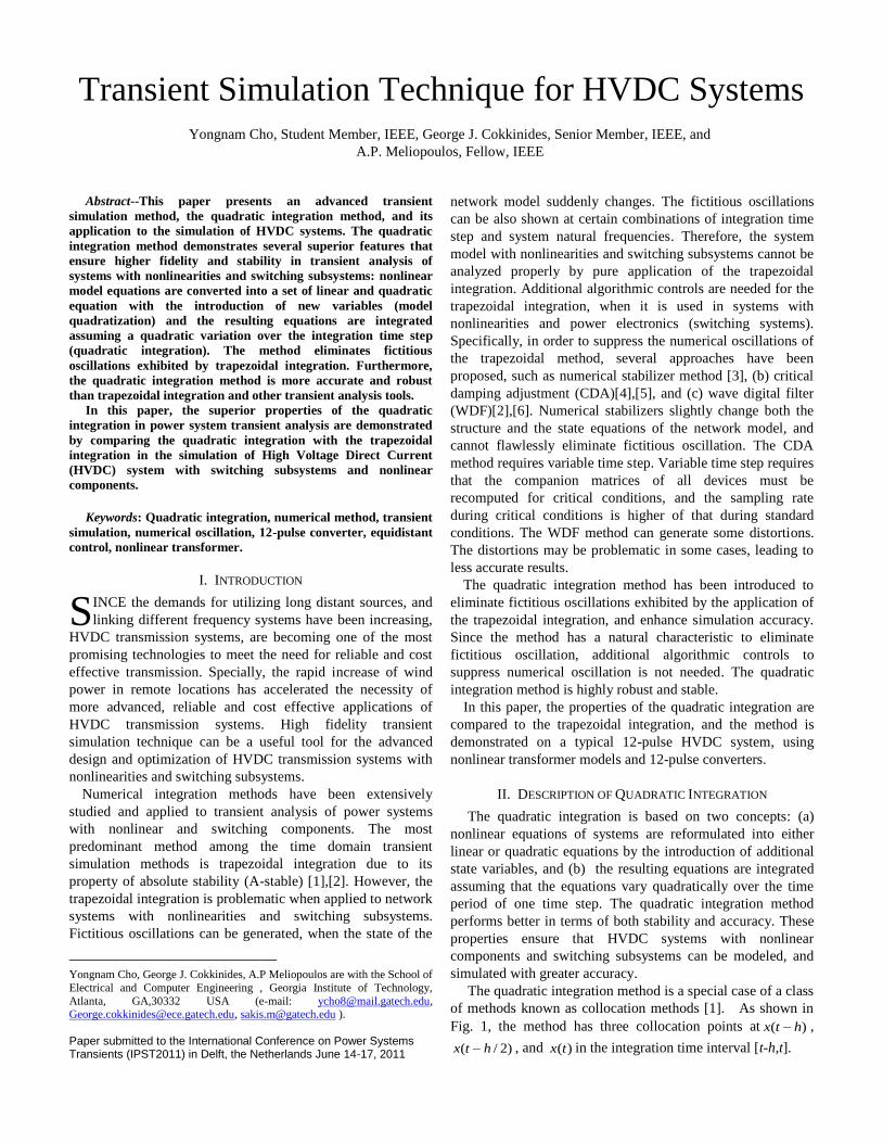
B. Three Phase Saturable Core Transformer
This section presents a method to quadratize nonlinear
equations. An example of a single phase saturable transformer
is used as it is illustrated in Fig.4.
)(1 tV
)(2 tV
)(3 tV
)(4 tV
)(1 ti
)(2 ti
)(3 ti
)(4 ti
1r 1L2r 2L
cr mL
)(tim
)(te )(tetn Fig. 4 A single phase saturable core transformer
The saturable core transformer is one of nonlinear
components. The core magnetizing reactance is modeled as a
nonlinear inductor with a (magnetizing) current that depends
on the core flux via a highly nonlinear equation (9):
))(()(0
0 tsigniti
n
m
(9)
The exponent n is typically 9 to 11 for usual magnetic material
used for transformers. The above equation can be quadratized
by introducing additional states and corresponding equations.
The number of additional states and equations depends on the
nonlinearity (exponent n). For simplicity, we show below the
application of this procedure in case the exponent is 5. This
case requires the introduction of two additional states, i.e. z1
and z2, and two additional equations. The system equations for
the single phase saturable transformer (including all equations,
i.e. linear and quadratized equations) are as follows.
)()()()()( 211111 tetvtvtidt
dLtir (10)
0)()( 21 titi (11)
)()()()()( 433232 tettvtvtidt
dLtir n (12)
0)()( 43 titi (13)
)()()()( 31 tetirttirtir mccc (14)
)()( tdt
dteo (15)
)()()(0 2
0
0 tzti
tim
(16)
)()(0 2
12 tztz (17)
)()(0 2
1
2
0 ttz (18)
A compact matrix form consisting of quadratic equations
and differential equations can be written for each phase of a
three phase transformer. Quadratic integration will yield the
algebraic companion form of the single phase transformer.
Subsequently, the algebraic companion form of a single phase
saturable transformer can be merged to form a three phase
saturable transformer in the same process as that of the six
pulse converter.
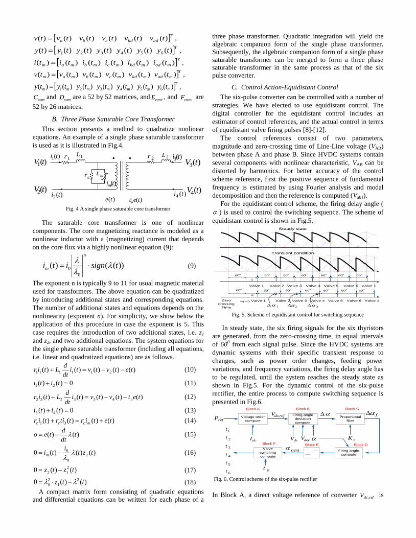
C. Control Action-Equidistant Control
The six-pulse converter can be controlled with a number of
strategies. We have elected to use equidistant control. The
digital controller for the equidistant control includes an
estimator of control references, and the actual control in terms
of equidistant valve firing pulses [8]-[12].
The control references consist of two parameters,
magnitude and zero-crossing time of Line-Line voltage (VAB)
between phase A and phase B. Since HVDC systems contain
several components with nonlinear characteristic, VAB can be
distorted by harmonics. For better accuracy of the control
scheme reference, first the positive sequence of fundamental
frequency is estimated by using Fourier analysis and modal
decomposition and then the reference is computed (Vab1).
For the equidistant control scheme, the firing delay angle (
) is used to control the switching sequence. The scheme of
equidistant control is shown in Fig.5.
Zero
crossing
Time
Valve 1 Valve 2 Valve 3 Valve 4 Valve 5 Valve 6 Valve 1
o60
`0
0wt
Valve 1 Valve 2 Valve 3 Valve 4 Valve 5 Valve 6 Valve 1
1
o60o60o60o60o60 o60
o60o60 o60 o60 o60 o60
2 3
Transient condition
Steady state
o60
Fig. 5. Scheme of equidistant control for switching sequence
In steady state, the six firing signals for the six thyristors
are generated, from the zero-crossing time, in equal intervals
of 600 from each signal pulse. Since the HVDC systems are
dynamic systems with their specific transient response to
changes, such as power order changes, feeding power
variations, and frequency variations, the firing delay angle has
to be regulated, until the system reaches the steady state as
shown in Fig.5. For the dynamic control of the six-pulse
rectifier, the entire process to compute switching sequence is
presented in Fig.6.
6
5
4
3
2
1
t
t
t
t
t
t
Block C
Voltage order
computerefP
dcI
Firing angle
deviation
compute
refdcV ,
dcV
Block A
fProportional
filter
Block B
cKdocV
Firing angle
compute
Valve
switching
compute
nextBlock EBlock F Block D
ot
( A )
Fig. 6. Control scheme of the six-pulse rectifier
In Block A, a direct voltage reference of converter refdcV , is
computed by dividing reference power refP into measured
direct current dcI .With the voltage reference, a deviation of
firing angle is calculated in Block B as follows:
dcccddc IKVV cos0 (19)
sin0cdVV , (20)
sin0cdV
V
dcref VVV . (21)
Where dcV is the measured direct voltage, cdV 0 is no-load
direct voltage at converter side, and cK is the equivalent
commutation resistance. It is obvious that the relationship
between direct voltage and firing angle is inherently nonlinear
as shown in (19). However, as shown in (21), the linear
relation between the deviations of both firing angle and direct
voltage exists, and the digital controller can linearly regulate
the six-pulse converter. In the next Block is
proportionally filtered with cf K , so that large
changes (jumps) in firing angle are avoided and the digital
controller can ensure smooth transitions and robust and stable
operation. A new firing angle next is calculated in Block D by
summing present firing angle and filtered deviation of firing
angle, and the new firing angle is bounded (for example
between o5 and o85 ) to prevent switching misfires in Block
E. With the new firing angle next and zero crossing time 0t
from DSP, Block F sequentially generates the firing pulses for
six valves. The mathematical notation is as follow:
Valve k : )6( 00 f
kttt delayk (22)
Where the time delay is calculated as 0)360/( Ttdelay , 0T
is fundamental period, 0f is fundamental frequency, and k
assumes integer values from 1 to 6.
The main idea of the digital controller for an inverter is very
similar to the rectifier controller, and only the differences in
firing delay angle has to be computed from the extinction
angle ( ) as follows.
diiiddi IKVV cos0 (23)
sin0idVV (24)
sin0idV
V
(25)
dcref VVV (26)
next (27)
nextnext
0180 (28)
Where diV is the measured direct voltage at the inverter side,
idV 0is no-load direct voltage at inverter, iK is equivalent
commutation resistance, and is commutation angle.
III. COMPARISON OF TRAPEZOIDAL AND QUADRATIC
INTEGRATION
A. Accuracy Comparison
Accuracy is an important characteristic of numerical
integration methods, since the reliability of power transient
analysis depends on it. In this paper, the accuracy of the
quadratic integration is compared with that of the trapezoidal
integration. The shaded parts of Fig.7 show symbolically and
exaggerated the integration error of both methods, and the
accuracy of solutions by the applications of both methods is
depended on these integration errors.
Fig. 7. Integration error of both methods.
( (A) quadratic integration, and (B) trapezoidal integration )
The truncation error is represented as follows (since the
trapezoidal integration is order two accurate and the quadratic
integration is order four accurate [1]):
)( 2hOE ltrapezoida and )( 4hOEquadratic over the interval [t-h,
t], where E denotes the truncation error, and h is the time step.
That is, the dominant error per step of trapezoidal integration
is proportional to h2 and that of the quadratic integration is
proportional to h4.
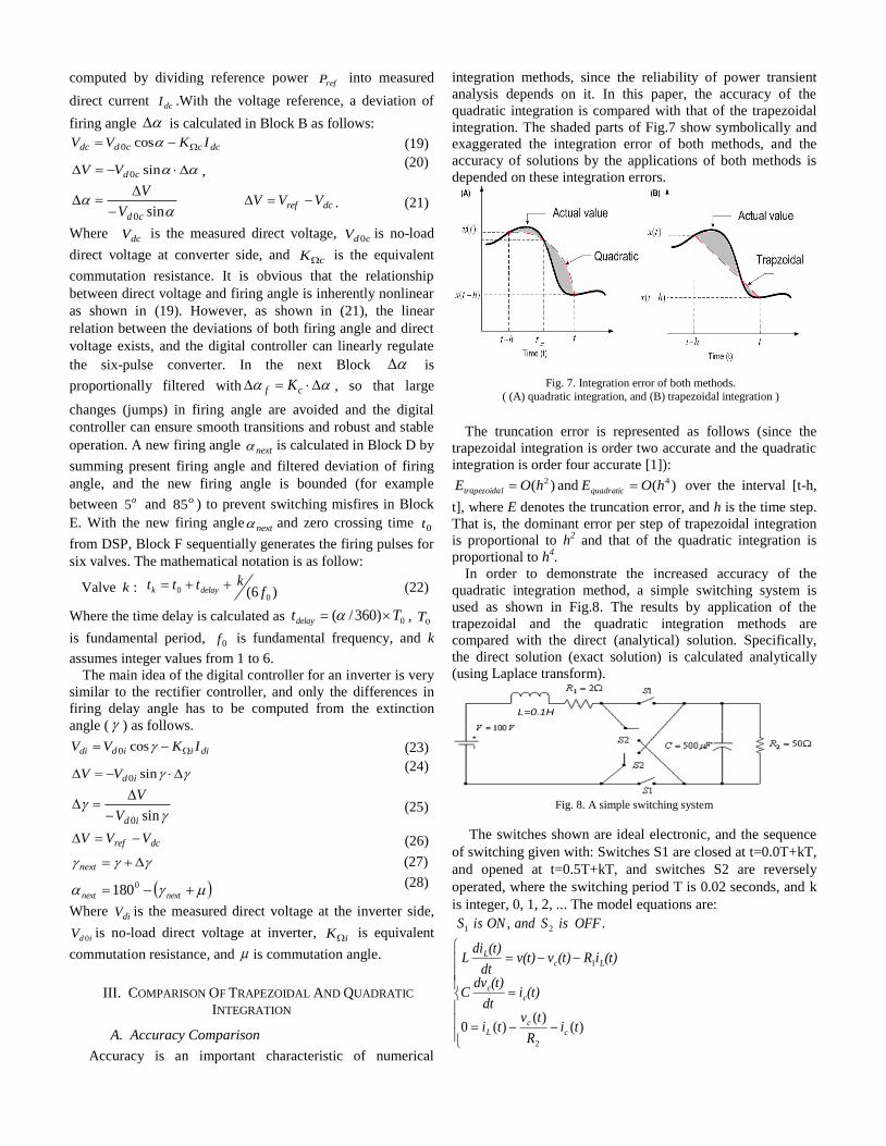
In order to demonstrate the increased accuracy of the
quadratic integration method, a simple switching system is
used as shown in Fig.8. The results by application of the
trapezoidal and the quadratic integration methods are
compared with the direct (analytical) solution. Specifically,
the direct solution (exact solution) is calculated analytically
(using Laplace transform).
L=0.1H
Fig. 8. A simple switching system
The switches shown are ideal electronic, and the sequence
of switching given with: Switches S1 are closed at t=0.0T+kT,
and opened at t=0.5T+kT, and switches S2 are reversely
operated, where the switching period T is 0.02 seconds, and k
is integer, 0, 1, 2, ... The model equations are:
)()(
)(0
.,
2
1
21
tiR
tvti
(t)idt
(t)dvC
(t)iR(t)vv(t)dt
(t)diL
OFFisSandONisS
cc
L
cc
LcL

.
)()(
)(0
,
2
1
21
tiR
tvti
(t)idt
(t)dvC
(t)iR(t)vv(t)dt
(t)diL
ONisSandOFFisS
cc
L
cc
LcL
Fig.9 shows the results (inductor current and the capacitor
voltage) from the direct analytical solution. The results by
application of the trapezoidal and quadratic integration
methods they appear to be similar in form as the waveforms of
Fig.9. In order to show the error clearly, Fig 10 shows the
absolute errors of both numerical methods during last 0.1
second and for two different integration time steps.
Fig. 9. Analytical simulation results
0.5 0.51 0.52 0.53 0.54 0.55 0.56 0.57 0.58 0.59 0.6
(Sec)
3105
3103
4109.1
4103.1
9107
9105.4
10103
10105.1
Time
Absolute Error of Trapezoidal (Time interval is 50 micro second)
Absolute Error of Trapezoidal (Time interval is 10 micro second)
Absolute Error of Quadratic (Time interval is 50 micro second)
Absolute Error of Quadratic (Time interval is 10 micro second)
Fig. 10. Absolute error of the inductor current by both numerical methods in
steady state
The absolute error is defined as:
)()( titierror numericalactual (29)
where iactual is actual inductor current calculated by the
Laplace transform, and inumerical is inductor current by
applications of the trapezoidal and quadratic integration. Note
that the absolute errors of the quadratic integration are about
six orders of magnitude smaller than the errors of the
trapezoidal integration. The example shows clearly the
substantially higher accuracy of the quadratic integration
method as compared to the trapezoidal integration. The
computational cost of the quadratic integration is almost twice
as much as that of the trapezoidal integration with the same
time step. However, the quadratic integration with time step of
50 micro-seconds as compared to the trapezoidal integration
with time step 10 microseconds offers more accurate
simulation results (more than three orders of magnitude) at a
fraction of the execution time (about 50% of the execution
time of trapezoidal integration).
B. Numerical Oscillation Comparison
Power transient analysis by application of Trapezoidal
integration has been suffered from numerical oscillations
especially in systems with nonlinearities and switching
subsystems. The root cause of the fictitious oscillations is well
known. The accuracy of the trapezoidal and quadratic
integration methods has been studied and reported in previous
publications [1], [3]. The possibility of fictitious oscillatory
solution can be studied from the general form of the numerical
solution of simple dynamical systems. Consider for a example
a first order dynamical system:
axdt
dx , where 0a . (30)
The physical system is stable, since 0a . Therefore the direct
analytical solution is also stable. The numerical solution using
trapezoidal integration is:
)(2
2)( htx
z
ztx
, where ahz , and h is positive. (31)
If the integration time step is so selected as to 2z , the
numerical solution for )(tx will oscillate around the true
values. Because the method is absolutely stable, the true
values can be approximated by filtering the oscillations. The
numerical solution using the quadratic integration, after
eliminating the mid-point, xm , is:
)(612
612)(
2
2
htxzz
zztx
(32)
where ahz , and h is positive.
Note that in the numerical solution (32) the coefficient cannot
become negative for any selection of the integration time step
(a is negative and h is positive). Therefore, the quadratic
integration is free of fictitious oscillations as compared to the
trapezoidal integration.
To demonstrate numerical oscillations graphically, the six
pulse converter model of Fig.2 is simulated with three
methods and with an appropriately selected integration time
step (same for all methods): (a) purely trapezoidal integration,
(b) trapezoidal integration with the numerical stabilizer
method, and (c) purely quadratic integration. The results are
shown in Fig.11.
2.939 2.948 2.958 2.967 2.976 2.986 2.995 2.939 2.948 2.958 2.967 2.976 2.986 2.995
2.939 2.948 2.958 2.967 2.976 2.986 2.995 2.939 2.948 2.958 2.967 2.976 2.986 2.995
Time (Second) Time (Second)
Time (Second) Time (Second)
196.0
0.0
-196.0
196.0
0.0
-196.0
8.91
0.0
-8.91
8.91
0.0
-8.91
Vol
tage
(M
V)
Vol
tage
(M
V)
Vol
tage
(K
V)
Vol
tage
(K
V)
(A) (B)
(C) (D)
Fig. 11. Line-Line voltage between Phase A and phase B of the six-pulse
converter. ((A) Purely trapezoidal, (B) Filtered waveform of (A), (C)
Trapezoidal with numerical stabilizer, and (D) Quadratic integration)
Trace (A) is the Line-Line voltage (A-B) solution using the
trapezoidal integration and trace B is the filtered version of
this solution. The results clearly demonstrate the existence of
fictitious oscillations around the true solution of the system.
Trace (C) shows the solution when numerical stabilizers are
used in the trapezoidal integration. Trace (D) shows the
solution by application of the quadratic integration which is
free of fictitious oscillations.
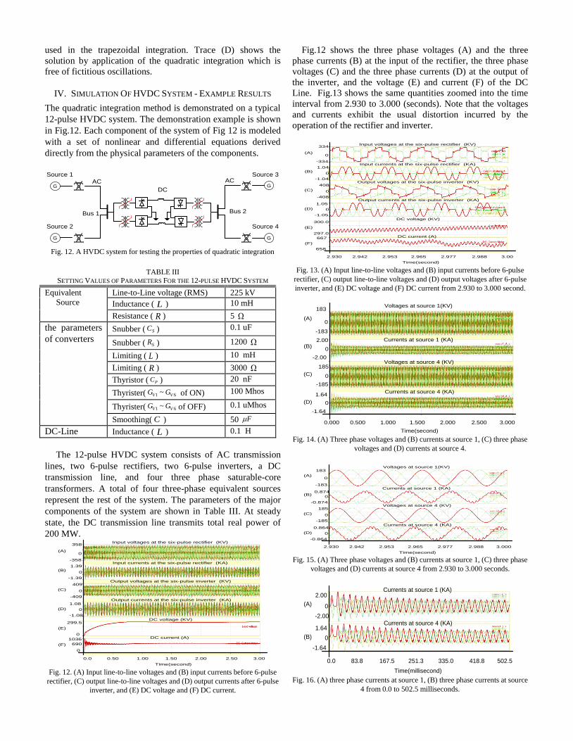
IV. SIMULATION OF HVDC SYSTEM - EXAMPLE RESULTS
The quadratic integration method is demonstrated on a typical
12-pulse HVDC system. The demonstration example is shown
in Fig.12. Each component of the system of Fig 12 is modeled
with a set of nonlinear and differential equations derived
directly from the physical parameters of the components.
G
G
G
G
Source 1
Source 2
Source 3
Source 4
Bus 1 Bus 2
AC AC
DC
Fig. 12. A HVDC system for testing the properties of quadratic integration
TABLE III
SETTING VALUES OF PARAMETERS FOR THE 12-PULSE HVDC SYSTEM
Equivalent
Source Line-to-Line voltage (RMS) 225 kV
Inductance ( L ) 10 mH
Resistance ( R ) 5
the parameters
of converters Snubber ( SC ) 0.1 uF
Snubber ( SR ) 1200
Limiting ( L ) 10 mH
Limiting ( R ) 3000
Thyristor ( PC ) 20 nF
Thyrister( 61 ~ VV GG of ON) 100 Mhos
Thyrister( 61 ~ VV GG of OFF) 0.1 uMhos
Smoothing( C ) 50 F
DC-Line Inductance ( L ) 0.1 H
The 12-pulse HVDC system consists of AC transmission
lines, two 6-pulse rectifiers, two 6-pulse inverters, a DC
transmission line, and four three phase saturable-core
transformers. A total of four three-phase equivalent sources
represent the rest of the system. The parameters of the major
components of the system are shown in Table III. At steady
state, the DC transmission line transmits total real power of
200 MW.
0.0 0.50 1.00 1.50 2.00 2.50 3.00
Time(second)
(A)
(B)
(C)
(D)
(E)
(F)
358
-358
0
1.39
-1.39
0
409
-409
0
1.08
-1.08
0
299.5
0
0
1036
690
Input voltages at the six-pulse rectifier (KV)
Input currents at the six-pulse rectifier (KA)
Output voltages at the six-pulse inverter (KV)
Output currents at the six-pulse inverter (KA)
DC voltage (KV)
DC current (A)
Fig. 12. (A) Input line-to-line voltages and (B) input currents before 6-pulse
rectifier, (C) output line-to-line voltages and (D) output currents after 6-pulse
inverter, and (E) DC voltage and (F) DC current.
Fig.12 shows the three phase voltages (A) and the three
phase currents (B) at the input of the rectifier, the three phase
voltages (C) and the three phase currents (D) at the output of
the inverter, and the voltage (E) and current (F) of the DC
Line. Fig.13 shows the same quantities zoomed into the time
interval from 2.930 to 3.000 (seconds). Note that the voltages
and currents exhibit the usual distortion incurred by the
operation of the rectifier and inverter.
2.930 2.942 2.953 2.965 2.977 2.988 3.00
Time(second)
(A)
(B)
(C)
(D)
(E)
(F)
334
-334
0
1.04
-1.04
0
408
-408
0
1.05
-1.05
0
300.0
297.0
658
667
Input voltages at the six-pulse rectifier (KV)
Input currents at the six-pulse rectifier (KA)
Output voltages at the six-pulse inverter (KV)
Output currents at the six-pulse inverter (KA)
DC voltage (KV)
DC current (A)
Fig. 13. (A) Input line-to-line voltages and (B) input currents before 6-pulse
rectifier, (C) output line-to-line voltages and (D) output voltages after 6-pulse
inverter, and (E) DC voltage and (F) DC current from 2.930 to 3.000 second.
0.000 0.500 1.000 1.500 2.000 2.500 3.000
Time(second)
(A)
(B)
(C)
(D)
183
-183
0
2.00
-2.00
0
185
-185
0
1.64
-1.64
0
Voltages at source 1(KV)
Currents at source 1 (KA)
Voltages at source 4 (KV)
Currents at source 4 (KA)
Fig. 14. (A) Three phase voltages and (B) currents at source 1, (C) three phase
voltages and (D) currents at source 4.
2.930 2.942 2.953 2.965 2.977 2.988 3.000
Time(second)
(A)
(B)
(C)
(D)
183
-183
0
0.874
-0.874
0
185
-185
0
0.864
-0.864
0
Voltages at source 1(KV)
Currents at source 1 (KA)
Voltages at source 4 (KV)
Currents at source 4 (KA)
Fig. 15. (A) Three phase voltages and (B) currents at source 1, (C) three phase
voltages and (D) currents at source 4 from 2.930 to 3.000 seconds.
0.0 83.8 167.5 251.3 335.0 418.8 502.5
Time(millisecond)
(A)
(B)
2.00
-2.00
0
1.64
-1.64
0
Currents at source 1 (KA)
Currents at source 4 (KA)
Fig. 16. (A) three phase currents at source 1, (B) three phase currents at source
4 from 0.0 to 502.5 milliseconds.

The graphs in Fig.14, 15 and 16 show (A) three phase
voltages and (B) currents at source 1, (C) three phase voltages
and (D) current at source 4. Close examination of the
waveforms show the presence of inrush currents during the
transient period which decay and become negligible at steady
state. The shape of the current waveforms in Fig.15 are closer
to sinusoidal as compared to the currents at the input of the
rectifier or the output of the inverter as expected. Another example is shown in Fig.17 and 18. In the example
we simulate a HVDC transmission system in steady state and
a step change order in power. Specifically, while the system
was operating at 200 MW of transmission through the HVDC
transmission line, a power change order of 100 MW (for a
total of 300 MW) is provided at time 3.5 seconds. The
response of the system is shown in the above mentioned
figures. Note that DC current and voltage transit very fast to
the new operating point. The firing angles (extinction angles,
etc.) of the four 6-pulse converters are automatically regulated
to meet the power order. In this simulation, we demonstrate
that the system can respond very fast to the power order
change. In real systems the power order will be in the form of
a power ramp that will result in smoother transitions of the
operating point.
0.0 1.17 2.33 3.50 4.67 5.83 7.00
Time(second)
(A)
(B)
(C)
(D)
(E)
(F)
358
-358
0
1.39
-1.39
0
409
-409
0
1.08
-1.08
0
567.0
0
0
1036
Input voltages at the six-pulse rectifier (KV)
Input currents at the six-pulse rectifier (KA)
Output voltages at the six-pulse inverter (KV)
Output currents at the six-pulse inverter (KA)
DC voltage (KV)
DC current (A)
Fig. 17. (A) Input voltages and (B) input voltages before 6-pulse rectifier, (C)
output voltages and (D) output voltages after 6-pulse inverter, and (E) DC
voltage and (F) DC current.
6.930 6.942 6.953 6.965 6.977 6.988 7.00
Time(second)
(A)
(B)
(C)
(D)
(E)
(F)
335
-335
0
0.728
-0.728
0
374
-374
0
0.759
-0.759
0
552.7
552.2
541.2
543.7
Input voltages at the six-pulse rectifier (KV)
Input currents at the six-pulse rectifier (KA)
Output voltages at the six-pulse inverter (KV)
Output currents at the six-pulse inverter (KA)
DC voltage (KV)
DC current (A)
Fig. 18. (A) Input voltages and (B) input voltages before 6-pulse rectifier, (C)
output voltages and (D) output voltages after 6-pulse inverter, and (E) DC
voltage and (F) DC current from 2.930 to 3.000 second.
V. CONCLUSIONS
This paper presented an advanced time domain method and
its application on a HVDC transmission system. The proposed
quadratic integration method is order four accurate.
Simulation results are more accurate than those by application
of the trapezoidal integration method. The quadratic
integration method eliminates fictitious oscillations, accurately
models nonlinear subsystems such as saturable-core
transformers and accurately models the operation of switching
subsystems. The proposed method is well suited for high
fidelity simulation of complex HVDC systems.
VI. REFERENCES
[1] A. Meliopoulos, G. Cokkinides, and G. Stefopoulos, “Quadratic integration method,” in Proceedings of the 2005 International Power
System Transients Conference (IPST 2005). Citeseer, pp. 19–23.
[2] M. Roitman and P. S. R. Diniz, "Simulation of non-linear and switching elements for transient analysis based on wave digital filters," IEEE
Trans. on Power Delivery, vol. 11, no. 4, pp. 2042-2048, Oct. 1996.
[3] W. Gao, E. Solodovnik, R. Dougal, G. Cokkinides, and A. Meliopoulos, “Elimination of numerical oscillations in power system dynamic
simulation,” in Applied Power Electronics Conference and Exposition,
2003 APEC’03. Eighteenth Annual IEEE, vol. 2, 2003. [4] J.Lin,J.R. Marti-“Implementation of the CDA Procedure in the EMTP”-
IEEE Transaction on Power Systems, V.5, n.2,pp.394-402, May 90.
[5] S N Hong, C R Liu, Z Q Bo, and A Klimek, “ Elimination of Numerical Oscillation of Dynamic Phasor in HVDC system Simulation,” in Power
and Energy Society General meeting,PES’09.IEEE,pp1-5,July 2009.
[6] M Roitman, P s R Diniz-“ Power systems simulation based on Wave Digital filters” IEEELPES 1995 Summer Meeting, paper 95 SM 400-2
PWRD, Jul95.
[7] A.P.Sakis Meliopoulos, George J.Cokkinides, George. Stefopoulos, “Symbolic integration of dynamical systems by collocation methods,” in
Proc. 2005. IEEE Power Engineering Society General Meeting, Vol. 1
pp. 817 - 822. [8] A. Ekstrom and G. Liss, “A refined HVDC control system,” IEEE
Transactions on Power Apparatus and Systems, pp. 723–732, 1970.
[9] R. Simard and V. Rajagopalan, “Economical Equidistant Pulse Firing Scheme for Thyristorized DC Drives,” IEEE Transactions on Industrial
Electronics and Control Instrumentation, pp. 425–429, 1975.
[10] S. Bhat, “Novel equidistant digital pulse firing schemes for three-phase thyristor converters,” International Journal of Electronics, vol. 50, no. 3,
pp. 175–182, 1981.
[11] J. Ainsworth, “The Phase-Locked Oscillator: A New Control System for Controlling Static Convertors,” IEEE Transactions on Power Apparatus
and Systems, pp. 859–865, 1968.
[12] N. Mohan, T. Undeland, and W. Robbins, Power electronics: converters, applications, and design. Wiley India, 2007.