transient thermal effects in alpine permafrost - the cryosphere

The Cryosphere, 3, 85–99, 2009www.the-cryosphere.net/3/85/2009/© Author(s) 2009. This work is distributed underthe Creative Commons Attribution 3.0 License.

The Cryosphere

Transient thermal effects in Alpine permafrost

J. Noetzli and S. Gruber

Glaciology, Geomorphodynamics and Geochronology, Department of Geography, University of Zurich, Switzerland

Received: 26 February 2008 – Published in The Cryosphere Discuss.: 2 April 2008Revised: 9 March 2009 – Accepted: 27 March 2009 – Published: 27 April 2009

Abstract. In high mountain areas, permafrost is importantbecause it influences the occurrence of natural hazards, be-cause it has to be considered in construction practices, andbecause it is sensitive to climate change. The assessment ofits distribution and evolution is challenging because of highlyvariable conditions at and below the surface, steep topog-raphy and varying climatic conditions. This paper presentsa systematic investigation of effects of topography and cli-mate variability that are important for subsurface temper-atures in Alpine bedrock permafrost. We studied the ef-fects of both, past and projected future ground surface tem-perature variations on the basis of numerical experimenta-tion with simplified mountain topography in order to demon-strate the principal effects. The modeling approach appliedcombines a distributed surface energy balance model and athree-dimensional subsurface heat conduction scheme. Re-sults show that the past climate variations that essentially in-fluence present-day permafrost temperatures at depth of theidealized mountains are the last glacial period and the ma-jor fluctuations in the past millennium. Transient effectsfrom projected future warming, however, are likely largerthan those from past climate conditions because larger tem-perature changes at the surface occur in shorter time peri-ods. We further demonstrate the accelerating influence ofmulti-lateral warming in steep and complex topography fora temperature signal entering the subsurface as compared tothe situation in flat areas. The effects of varying and un-certain material properties (i.e., thermal properties, porosity,and freezing characteristics) on the subsurface temperaturefield were examined in sensitivity studies. A considerableinfluence of latent heat due to water in low-porosity bedrockwas only shown for simulations over time periods of decadesto centuries. At the end, the model was applied to the to-

Correspondence to:J. Noetzli([email protected])

pographic setting of the Matterhorn (Switzerland). Resultsfrom idealized geometries are compared to this first exampleof real topography, and possibilities as well as limitations ofthe model application are discussed.

1 Introduction

In Alpine environments, permafrost is a widespread thermalsubsurface phenomenon. Permafrost is defined as materialof the lithosphere that remains at or below 0◦C for at leasttwo consecutive years (e.g., Brown and Pewe 1973, Wash-burn 1979). Its possible warming and degradation in con-nection with climate change is regarded as a decisive factorinfluencing the stability of steep rock faces (e.g., Haeberliet al., 1997; Davies et al., 2001; Noetzli et al., 2003; Gru-ber and Haeberli, 2007). It is therefore important to assessthe impact of climate change on mountain permafrost for theunderstanding of natural hazards and for construction prac-tices (Haeberli, 1992; Harris et al., 2001; Romanovsky etal., 2007), especially in densely populated areas such as theEuropean Alps. Further, permafrost influences Alpine land-scape evolution, hydrology, and it is monitored in the scopeof climate observing systems (e.g., Global Terrestrial Net-work for Permafrost, GTN-P, within the Global Climate Ob-serving System, GCOS). The quantification of temperaturechanges and the discernment of zones that are sensitive topermafrost degradation require knowledge of the spatial dis-tribution of subsurface temperatures as well as of their evo-lution. Even though measured temperature profiles in bore-holes enable an initial assessment of temperature changes(e.g., Isaksen et al., 2007; PERMOS, 2007), they cannotbe used for an extrapolation in space or time in a simpleand straightforward way in high mountains (cf. Gruber etal., 2004c). The extreme topography in these areas leads tospatially highly variable surface conditions and distortionsof both, direction and density of heat flow in the subsurface.

Published by Copernicus Publications on behalf of the European Geosciences Union.

http://creativecommons.org/licenses/by/3.0/

86 J. Noetzli and S. Gruber: Transient thermal effects in Alpine permafrost

The understanding of three-dimensional and transient sub-surface temperature fields below steep topography can beimproved by numerical modeling that accounts for two- andthree-dimensional effects (e.g., Safanda, 1999; Kohl et al.,2001; Wegmann et al., 1998).

Noetzli et al. (2007b) have shown that in complex topog-raphy ground surface temperatures (GST) alone do not suffi-ciently indicate the thermal conditions at depth (when speak-ing of “at depth” in this paper, we refer to depths deeper thanthe zero annual amplitude – ZAA): Because of existing lat-eral heat fluxes, permafrost can occur at locations with pos-itive GST even if conditions are stationary. Stationary con-ditions, however, do not describe the situation found in na-ture since transient effects of past climate periods addition-ally modify the subsurface temperature field. In the SwissAlps, permafrost thickness ranges from a few meters up toseveral hundreds of meters below the highest peaks (such asthe Monte Rosa massif; Luthi and Funk, 2001), and timescales involved in deep permafrost changes can be in therange of millennia even without the retarding effect of latentheat (e.g., Lunardini, 1996; Kukkonen and Safanda, 2001;Mottaghy and Rath, 2006). Consequently, the influence ofpast cold periods such as the last Ice Age are likely to persistin permafrost temperatures in the interior of high mountains(Haeberli et al., 1984, Kohl, 1999; Kohl and Gruber, 2003).The more recent but smaller 20th century warming (Haeberliand Beniston, 1998; Beniston, 2005) currently affects groundtemperatures in the upper decameters. That is, a realisticsimulation of today’s thermal state of mountain permafrostcannot be based on current GST alone, but it is necessary toinitialize the model far enough in the past. A correspondinginitialization procedure has to include the past climate varia-tions that influence current subsurface temperatures. Further,the modeling of transient temperature fields is essential to as-sess possible permafrost temperatures in the coming decadesand centuries.

The combined effects of steep topography and transientpaleoclimatic signals on the subsurface temperature fieldsin the interior of Alpine peaks have not been systematicallystudied so far. In this paper, we first analyze how big the in-fluence of past climate conditions is on the present-day ther-mal state of mountain permafrost. And secondly, we con-sider a simplified scenario of future climate change in orderto estimate their effect. Our study is based on numerical ex-perimentation with simplified topography and typical valuesof surface and subsurface conditions because the situation innature is highly variable and complex. The results of suchidealized simulations can be used to identify the principaleffects and will contribute to our understanding of the three-dimensional distribution of mountain permafrost, its thermalstate today, and its possible evolution in the future. Theyshould be seen as a step towards assessing natural and morecomplicated situations. Results will also be useful to decideon the initialization procedure required for the modeling ofpermafrost temperatures in high-mountains. At the end, the

model is applied to the topographic setting of the Matterhorn(Switzerland). Results from idealized geometries are com-pared to this first example of real topography, and possibili-ties as well as important limitations of the model applicationsare discussed.

2 Background and approach

2.1 Background

Many studies point to significant temperature depressions inthe deeper subsurface, which are caused by past cold climateconditions (e.g., Haeberli et al., 1984; Safanda and Rajver,2001). That is, actual subsurface temperatures are colderthan for a stationary temperature field that corresponds tocurrent climate conditions. The depth to which a ground sur-face temperature variation is perceivable is determined by itsamplitude and duration, as well as by the thermal proper-ties of the subsurface. In modeling studies, such temperatureanomalies are usually computed as deviations of actual ther-mal conditions from equilibrium conditions (e.g., Pollak andHuang, 2000; Beltrami et al., 2005). In a first approach, theycan be calculated by superposition of stepwise temperaturechanges using analytical heat transfer solutions (e.g., Birch,1948; Carslaw and Jaeger, 1959). Based on this technique,an assumed 10◦C cooler surface temperature during the lastPleistocene Ice Age (ca. 70–100 ky BP) still causes a tem-perature depression of more than 4◦C at a depth of 1000 m(Kohl, 1999). Haeberli et al. (1984) have estimated a groundtemperature depression from the last cold period of 5◦C at adepth of about 1000 to 1500 m for the Swiss Plateau.

A large number of studies exist that use measured temper-atures in deep boreholes to reconstruct past climatic condi-tions (e.g., Lachenbruch and Marshall, 1986; Pollak et al.,1998; Huang et al., 2000; Beltrami, 2001; Kukkonen andSafanda, 2001). Relating to such studies, past climate vari-ations that have a significant influence on current subsur-face temperatures can be identified. Climate reconstructionstudies are, however, typically based on data measured inboreholes that were drilled in flat areas and that are princi-pally subject to one-dimensional vertical heat transfer. Onlya few recent studies deal with the effect of past tempera-tures together with two- or three-dimensional topography.Kohl (1999) demonstrated that the transient temperature sig-nal can be modified by topography even at depths of morethan 1000 m. Case studies in permafrost areas in the SwissAlps (Wegmann et al., 1998; Luthi and Funk, 2001; Kohl andGruber, 2003) indicate that the long term climate history hasto be taken into account to realistically reproduce measuredtemperature fields and warming rates at depth. GST historiesconsidered in these studies reach back in time for 1200 yearsfor local case studies (Wegmann et al., 1998) and more than10 000 years for entire mountain massifs (Kohl et al., 2001;Luthi and Funk, 2001).

The Cryosphere, 3, 85–99, 2009 www.the-cryosphere.net/3/85/2009/

J. Noetzli and S. Gruber: Transient thermal effects in Alpine permafrost 87

2.2 Approach

The modeling of subsurface temperatures in high-mountainsis complex because temperature fields are significantly in-fluenced by (i) spatially variable GST, (ii) spatially vari-able properties of the subsurface, (iii) three-dimensional ef-fects caused by steep terrain geometry, and (iv) the evolu-tion of GST in the past. In this study, we used and furtherdeveloped the modeling procedure described by Noetzli etal. (2007a, b), which has been designed and validated (Noet-zli 2008, Noetzli et al., 2008) for use in steep mountain to-pography: A distributed surface energy balance model to cal-culate ground surface temperatures and a three-dimensionalheat-conduction model are combined for forward simulationof a subsurface temperature field (Fig. 1).

Heat transfer is mainly conductive in bedrock permafrostand is driven by the spatial and temporal temperature vari-ations at the surface and the heat flow from the interior ofthe earth. The distributed surface energy balance model usedenables a sound calculation of spatially variable surface tem-peratures in steep terrain (Gruber et al., 2004b). Further pro-cesses such as advection by fluid flow can, as a first approx-imation, be neglected (e.g., Kukkonen and Safanda, 2001).Accordingly, we considered a purely conductive transientthermal field with the modeled surface temperatures as up-per, and the geothermal heat flux as lower boundary condi-tion. More details on the models, their validation, and theirsettings are given in Sect. 3.

To account for the evolution of GST in the past, we ini-tialize the subsurface temperature field based on a prescribedGST history using a steady state solution for the GST con-ditions at the start time. We applied different GST histories,which we compiled based on published changes in air tem-peratures and the simplifying assumption that GST followthese changes closely. That is, effects from changes in othercomponents of the surface energy balance, snow cover, orsurface characteristics are not considered. Temporal vari-ations of surface temperatures penetrate downward with aconsiderable time lag and with amplitudes diminishing ex-ponentially with depth. In this study, we ignore seasonaltemperature variations, which may penetrate down to about10–15 m in solid and dry bedrock (Gruber et al., 2004a),and only consider long-term variations with time scales ofdecades to millennia, which influence temperatures at greaterdepth. Such long-term variations still occur on much shortertime scales than the geological processes that determine thegeothermal heat flow. The past climatologic variations aretherefore treated as transient effects of the upper boundariesin our model, and the lower basal heat flow boundary con-dition is kept constant (cf. Pollak and Huang, 2000). Thelack of information concerning the most important subsur-face characteristics that influence conductive heat transport(thermal properties, porosity, freezing characteristics, etc.) isapproached by using model assumptions based on sensitivitystudies.

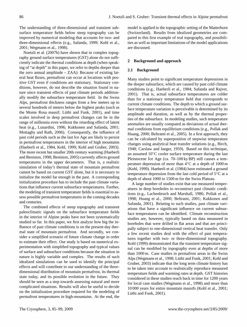
Fig. 1. Mean ground surface temperatures (MGST) are calculatedbased on a surface energy balance model (TEBAL). They are usedas upper boundary condition in a three-dimensional finite elementheat conduction scheme (within COMSOL) to compute the subsur-face temperature field. For transient simulations the evolution of thesurface temperatures is prescribed.

We performed the basic simulations for a simplified ridge,the most common feature comprising Alpine topography(cf. Noetzli et al., 2007). A ridge of 1000 m height wasset to an elevation of 3500 m a.s.l. and east-west orientation.Hence, it has a warm south-facing and a cold north-facingslope, which induces a subsurface temperature field withsteeply inclining isotherms in the uppermost part (cf. Fig. 3).A threshold for the slope of steep bedrock is often set at about37◦ (e.g., Gruber and Haeberli, 2007). Couloirs with thissteepness, however, can often contain a significant amount ofsnow or debris, and because we do not consider any surfacecover in the idealized settings, we set the slope value to 50◦.In order to study the influence of terrain geometry, we variedthe topographic factors (i.e., elevation and slope angle) of thetwo-dimensional ridge. Finally, we compared the results fora ridge topography to those for a flat and one-dimensionalplain and a three-dimensional mountain peak represented bya pyramid. The use of a distributed energy balance approachis not essential for the experimentation presented here, anda reasonable parameterization for GST would suffice. Formodel application to more complex topography, however, thespatial distribution of GST cannot be easily parameterizedand its sound calculation is crucial, because it drives the di-rection and magnitude of subsurface heat fluxes (Gruber etal., 2004c; Noetzli et al., 2007). For consistency and in or-der to demonstrate the entire modeling procedure, GST arecalculated based on the distributed energy balance model forsimulations with both, idealized and real topography.

3 Temperature modeling

3.1 Energy balance and rock surface temperatures

The TEBAL model (Topography and Energy BALance) sim-ulates distributed surface energy fluxes in complex terrainbased on observed climate time series, topography, and sur-face and subsurface information. The model is designed

www.the-cryosphere.net/3/85/2009/ The Cryosphere, 3, 85–99, 2009


Table 1. Surface and subsurface properties assumed in the experimentation runs.

Surface

Emissivity 0.96 Gruber et al., 2004cRougness 0.0001 m Gruber et al., 2004cAlbedo 0.2 Gruber et al., 2004c

Subsurface

Volum. heat capacity 2.0×106 J m−3 K−1 Cermak and Rybach, 1982; Wegmann et al., 1998Thermal conductivity 2.5 W K−1 m−1 Cermak and Rybach, 1982; Wegmann et al., 1998Porosity (saturated) 3% Wegmann et al., 1998

(Gruber, 2005; Stocker-Mittaz, 2002) and validated (Gru-ber, 2005; Gruber et al., 2004b; Noetzli et al., 2007b) for thecalculation of near-surface temperatures in steep rock slopesin the Alps and was successfully applied in previous studieson bedrock permafrost (e.g., Gruber et al., 2004a, b; Noet-zli et al., 2007b; Salzmann et al., 2007). Mean ground sur-face temperatures (MGST) are computed using gridded dig-ital elevation models (DEMs) of the topography consideredand with hourly climate time series from a high elevationmeteo station. In this paper, we used the data from Cor-vatsch at 3315 m a.s.l. in the Upper Engadine (Data source:MeteoSwiss) for the period 1990–1999 AD. We further ref-erence this period as “today” or “present”. Surface and sub-surface properties for bedrock were set to typical values ofAlpine rock according to Noetzli et al. (2007a; Table 1). Theinfluence of their possible variation was additionally assessedin sensitivity studies (cf. Sects. 4.1.2 and 4.2.2.) For simpli-fication purposes and because most steep rock slopes do notaccumulate a thick snow cover during winter, we neglect thesimulation of the snow cover for the numerical experiments.

3.2 Heat conduction and subsurface temperatures

As described above (Sect. 2.2), we considered a conduc-tive three-dimensional transient thermal field (Carslaw andJaeger, 1959) in an isotropic and homogeneous medium un-der complex topography. The thermal properties of the sub-surface were set based on published values (Cermak and Ry-bach, 1982; Wegmann et al., 1998; Safanda, 1999) (cf. Ta-ble 1).

Ice contained in the pore space and crevices delays the re-sponse to surface warming by the consumption of latent heat,which may influence the time and depth scales of permafrostdegradation by orders of magnitude even in low porosity rock(Wegmann et al., 1998; Romanovsky and Osterkamp, 2000;Kukkonen and Safanda, 2001). This effect can be handledin heat transfer models by introducing an apparent heat ca-pacity. We used the approach described by Mottaghy andRath (2006): The apparent heat capacity substitutes the heatcapacity in the heat transfer equation within the freezing in-tervalw. The freezing intervalw describes the temperature

range, where phase transition takes place and unfrozen wa-ter is present, and which relates to the steepness of the un-frozen water content curve. The parameterw makes it pos-sible to account for a variety of ground conditions (Mot-taghy and Rath, 2006): Values ofw typically range from0.5 K for material such as sand to 2 K for material such asbentonite (Anderson and Tice, 1972; Williams and Smith,1989), but information on bedrock material is sparse. Weg-mann (1998) found that most of the interstitial ice in the rockof the Jungfrau East Ridge, Switzerland, freezes at –0.3◦C,which indicates a small freezing interval with a steep curveand a low value ofw. A further important factor is the poros-ity of the material, for which we assumed 3% (volume frac-tion, saturated conditions) to be a reasonable value to inves-tigate the principal effects (cf. Wegmann et al., 1998).

The commercial finite-element (FE) modeling packageCOMSOL Multiphysics was used for forward modeling ofsubsurface rock temperatures (Noetzli et al., 2007a). Theheat conduction module included in this software has beensuccessfully used for the simulation of borehole temperatureprofiles in the Schilthorn ridge, Switzerland (Noetzli et al.,2008) and the Zugspitze, Germany (Noetzli, 2008). The FEmesh for the topographies was created with increasing verti-cal refinement from 250 m at depth to 10 m for elements clos-est to the surface. In order to avoid effects from the modelboundaries, a rectangle box of 2000 m height and thermal in-sulation at its sides was added below the geometry. The FEmesh consisted of ca. 1500 elements for a ridge, and of about25 000 elements for a pyramid. The lower boundary condi-tion was set to a uniform heat flux of 80 mW m−2 (Mediciand Rybach, 1995), and for the upper boundary conditionsthe modeled MGSTs were given. The model was run withtime-steps of 1 year for simulations over a period of morethan 1000 years, and with time steps of 10 days for shorterperiods. Sensitivity runs with higher refinement of the FEmesh, a lower boundary condition set at greater depth, andsmaller time steps did not considerably change any of the re-sults (i.e., the maximum absolute difference in modeled tem-peratures was below 0.1◦C).

The modeling procedure bases on the coupling of the dis-tributed energy balance model TEBAL with subsurface heat



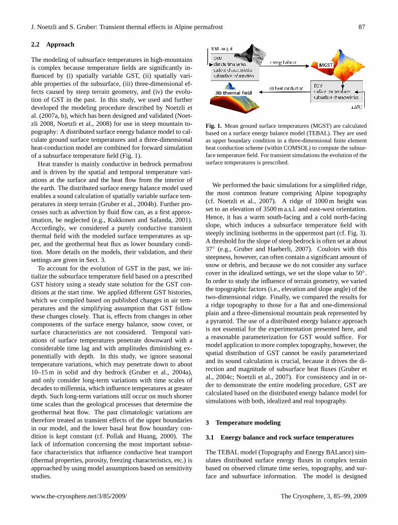
Fig. 2. For the initialization runs, surface temperature histories ofdiverse lengths and temporal resolutions were used. Based on theresults obtained, an initialization curve for further simulations wascompiled (thick dashed orange line). Scenarios were calculated as-suming a uniform linear warming of+3◦C/100 y. MW=MedievalWarmth, HCO=Holocene Climate Optimum, LIA=Little Ice Age.

conduction simulated in COMSOL. Because measurementsof entire three-dimensional temperature fields in mountainsare hardly feasible, three different validation steps have beentaken in order to gain confidence in the modeling results(Noetzli, 2008). They include: (1) comparison with field datameasured at or near the surface, (2) comparison with tem-perature profiles from boreholes, and (3) sensitivity studies.For (1) and (2) we refer to the detailed descriptions and re-sults presented in Gruber et al. (2004b), Noetzli et al. (2007),Noetzli (2008), and Noetzli et al. (2008). Sensitivity studiesto assess the uncertainties related to the lack of informationon subsurface properties and the surface temperature historyare part of this paper (cf. Sect. 4 for results).

3.3 Evolution of surface temperature

A wealth of literature exists on temperature reconstructionsfrom proxy data for global (Pollak et al., 1998; Huang etal., 2000; Jones and Mann, 2004), hemispheric (Jones et al.,1998; Petit et al., 1999), and regional scale (Patzelt, 1987;Isaksen et al., 2000; Casty et al., 2005) over the past centuriesand millennia. For the European Alps, temperature variationsare generally more pronounced with larger amplitudes com-pared to those averaged globally or for the Northern Hemi-sphere (Beniston et al., 1997; Pfister, 1999; Luterbacher etal., 2004). In the uppermost kilometers of the Earth’s crust,mainly the thermal effects of two events are prominent today(Haeberli et al., 1984): the temperature depression duringthe Pleistocene Ice Age and the sharp rise in temperaturesbetween the time of maximum glaciation (around 18 ky BP)and the beginning of the thermally more stable Holocene(around 10 ky BP). For the Holocene, the Climatic Optimum(HCO, ca. 5–6 ky BP), the Medieval Warmth (MW, ca. 800–

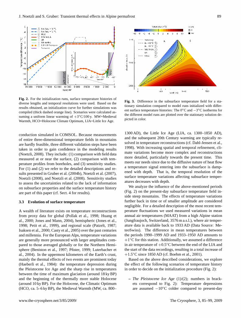
Fig. 3. Difference in the subsurface temperature field for a sta-tionary simulation compared to model runs initialized with differ-ent surface temperature histories: The 0◦C and−3◦C isotherms forthe different model runs are plotted over the stationary solution de-picted in color.

1300 AD), the Little Ice Age (LIA, ca. 1300–1850 AD),and the subsequent 20th Century warming are typically re-solved in temperature reconstructions (cf. Dahl-Jensen et al.,1998). With increasing spatial and temporal refinement, cli-mate variations become more complex and reconstructionsmore detailed, particularly towards the present time. Thismeets our needs since due to the diffusive nature of heat flowa temperature signal entering into the subsurface is damp-ened with depth. That is, the temporal resolution of thesurface temperature variations affecting subsurface temper-atures decreases with depth.

We analyze the influence of the above-mentioned periods(Fig. 2) on the present-day subsurface temperature field in-side steep mountains. The effects of temperature variationsfurther back in time or of smaller amplitude are considerednegligible. For a detailed description of the most recent tem-perature fluctuations we used measured variations in meanannual air temperatures (MAAT) from a high Alpine station(Jungfraujoch, Switzerland, 3576 m a.s.l.), where air temper-ature data is available back to 1933 AD (Data Source: Me-teoSwiss). The difference in mean temperatures betweenthe periods 1990–1999 AD and 1933–1950 AD amounts to+1◦C for this station. Additionally, we assumed a differencein air temperature of+0.5◦C between the end of the LIA andthe start of the data recordings, resulting in a total increase of+1.5◦C since 1850 AD (cf. Boehm et al., 2001).

Based on the above described considerations, we explorethe effect of the following scenarios of temperature historyin order to decide on the initialization procedure (Fig. 2):

– The Pleistocene Ice Age(1)/(2); numbers in brack-ets correspond to Fig. 2): Temperature depressionsare assumed−10◦C colder compared to present-day



temperatures (Patzelt, 1987), followed by a linear in-crease from the time of maximum glaciation (18 ky BP)to the beginning of the Holocene (10 ky BP). For theHolocene no temperature variations were considered.To assess the effect of colder estimates, we additionallyused a value of−15◦C (Haeberli et al., 1984).

– HCO (3): During the Holocene Climate Optimum sum-mer temperatures were approx. 1.5–3◦C warmer thantoday (Burga, 1991). Mean annual temperatures prob-ably were not as high, but to test the influence of thisperiod we assumed+2◦C.

– Past millennium (4): In contrast to e.g., vonRudloff (1980), newer studies conclude that air tem-peratures in Europe during the MW were probably notwarmer than or comparable to today (Hughes and Diaz,1994; Crowley and Lowery, 2000; Goosse et al., 2006).Yet, to estimate the possible influence of the MW weused 0.5◦C higher surface temperatures than at present.For the LIA, we assumed temperatures 1.5◦C lower(Boehm et al., 2001).

– Recent warming: We used a linear temperature increasefollowing the LIA (5) and, in addition, annual MAATvariations taken from Jungfraujoch meteodata (6).

Further, to asses the transient response of the subsurfacetemperature field to future warming, we used a warming sce-nario of the rock surface of+3◦C/100 y. This value hasbeen calculated as a mean warming of Alpine rock surfacesfrom 1982–2002 to 2071–2091, based on output from differ-ent Regional Climate Models, different emission scenarios,downscaling methods, and varying topographic settings bySalzmann et al. (2007). Since no information on the form ofthe increase (e.g., exponential) was deducted and uncertain-ties are high, we chose a linear increase. Based on this sim-ple scenario, the principal effects of the transient response ofbedrock temperatures can be investigated.

4 Transient temperature fields below idealizedtopography

4.1 Effects of past climatic conditions

If not indicated otherwise, results are discussed and visual-ized for a ridge cross section of 1000 m height with a maxi-mum elevation of 3500 m a.s.l., and a slope angle of 50◦; thesubsurface material is assumed homogenous and isotropic,and no latent heat is considered. Variations from these basicsettings are mentioned in the text and indicated in the fig-ures with checkboxes and corresponding abbreviations (i.e.,ini for initialized, lh for latent heat considered, andiso forisotropic subsurface conditions).

The stationary temperature field describes the generalcharacter of the subsurface temperature pattern of the ridge,

which does not fundamentally differ for temperatures re-sulting from initialized model runs. The latter, however,are lower for the entire thermal field and all GST historiesused. 0◦C and−3◦C-isotherms of temperature fields ini-tialized with different GST histories are compared to sta-tionary conditions with current GST in Fig. 3: Accordingto the definition of permafrost, the 0◦C isotherm stands forthe schematic permafrost boundary in the idealized mountainridge, whereas the−3◦C isotherm relates to the temperaturedistribution inside the schematic permafrost body. The re-sulting temperature depressions from the last Ice Age (1) isin the range of−0.5◦C for the upper half of the geometry,and in the range of−2.5◦C for the lower part. When assum-ing colder GST in the last Ice Age (2) these values amountto −1◦C and−4◦C, respectively. Simulating the GST vari-ations during the Holocene (4) results in additionally lowertemperatures: On the one hand, the LIA (5) is perceivabledown to about 250 m depth. On the other hand, deeper partsare modeled colder because (1) and (2) do not consider thatpresent-day GST are somewhat higher than Holocene aver-age. The effect of the HCO (3) is below 0.1◦C for the entiregeometry, and results are therefore not displayed in Fig. 3.Results for GST history (6) do not notably differ from (5) andare not shown, either. Based on the results from (1) to (6), wecompiled GST history (7), which accounts for the variationsfor which a significant influence was shown above. Althoughwe use highly idealized conditions in the experiments, it canbe assumed that these are the most important variations thatinfluence the subsurface thermal field in high mountains, be-cause thermal properties and size of the major part of Alpinetopography does not essentially differ from the geometriesused: We considered the cold temperatures during the lastIce Age (1) and the major fluctuations in the past millennium(4). GST history (7) is used for all subsequent calculations inthis study and corresponding temperature fields are referredto as “initialized” or “transient”.

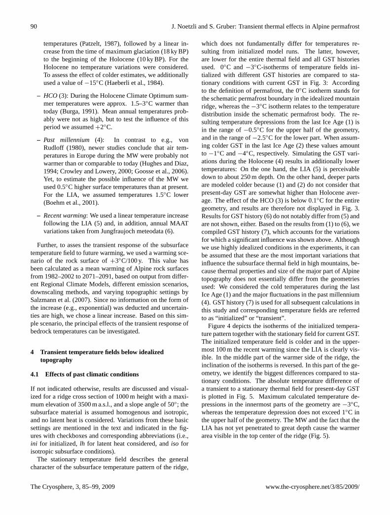
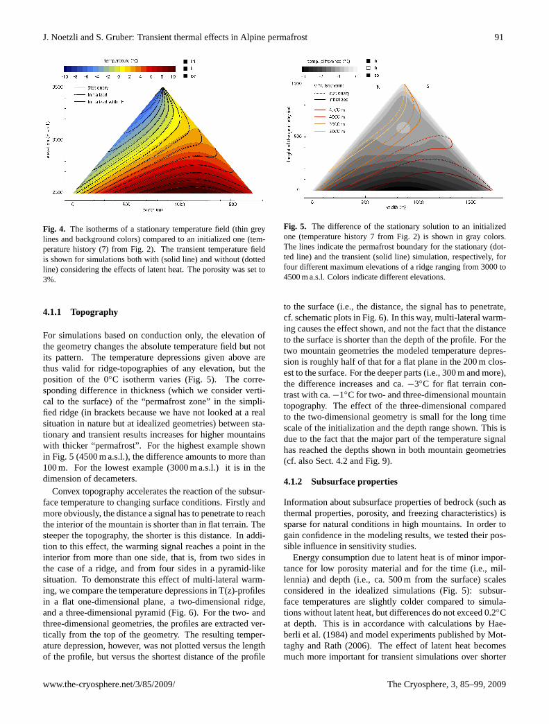
Figure 4 depicts the isotherms of the initialized tempera-ture pattern together with the stationary field for current GST.The initialized temperature field is colder and in the upper-most 100 m the recent warming since the LIA is clearly vis-ible. In the middle part of the warmer side of the ridge, theinclination of the isotherms is reversed. In this part of the ge-ometry, we identify the biggest differences compared to sta-tionary conditions. The absolute temperature difference ofa transient to a stationary thermal field for present-day GSTis plotted in Fig. 5. Maximum calculated temperature de-pressions in the innermost parts of the geometry are−3◦C,whereas the temperature depression does not exceed 1◦C inthe upper half of the geometry. The MW and the fact that theLIA has not yet penetrated to great depth cause the warmerarea visible in the top center of the ridge (Fig. 5).



Fig. 4. The isotherms of a stationary temperature field (thin greylines and background colors) compared to an initialized one (tem-perature history (7) from Fig. 2). The transient temperature fieldis shown for simulations both with (solid line) and without (dottedline) considering the effects of latent heat. The porosity was set to3%.

4.1.1 Topography

For simulations based on conduction only, the elevation ofthe geometry changes the absolute temperature field but notits pattern. The temperature depressions given above arethus valid for ridge-topographies of any elevation, but theposition of the 0◦C isotherm varies (Fig. 5). The corre-sponding difference in thickness (which we consider verti-cal to the surface) of the “permafrost zone” in the simpli-fied ridge (in brackets because we have not looked at a realsituation in nature but at idealized geometries) between sta-tionary and transient results increases for higher mountainswith thicker “permafrost”. For the highest example shownin Fig. 5 (4500 m a.s.l.), the difference amounts to more than100 m. For the lowest example (3000 m a.s.l.) it is in thedimension of decameters.

Convex topography accelerates the reaction of the subsur-face temperature to changing surface conditions. Firstly andmore obviously, the distance a signal has to penetrate to reachthe interior of the mountain is shorter than in flat terrain. Thesteeper the topography, the shorter is this distance. In addi-tion to this effect, the warming signal reaches a point in theinterior from more than one side, that is, from two sides inthe case of a ridge, and from four sides in a pyramid-likesituation. To demonstrate this effect of multi-lateral warm-ing, we compare the temperature depressions in T(z)-profilesin a flat one-dimensional plane, a two-dimensional ridge,and a three-dimensional pyramid (Fig. 6). For the two- andthree-dimensional geometries, the profiles are extracted ver-tically from the top of the geometry. The resulting temper-ature depression, however, was not plotted versus the lengthof the profile, but versus the shortest distance of the profile

Fig. 5. The difference of the stationary solution to an initializedone (temperature history 7 from Fig. 2) is shown in gray colors.The lines indicate the permafrost boundary for the stationary (dot-ted line) and the transient (solid line) simulation, respectively, forfour different maximum elevations of a ridge ranging from 3000 to4500 m a.s.l. Colors indicate different elevations.

to the surface (i.e., the distance, the signal has to penetrate,cf. schematic plots in Fig. 6). In this way, multi-lateral warm-ing causes the effect shown, and not the fact that the distanceto the surface is shorter than the depth of the profile. For thetwo mountain geometries the modeled temperature depres-sion is roughly half of that for a flat plane in the 200 m clos-est to the surface. For the deeper parts (i.e., 300 m and more),the difference increases and ca.−3◦C for flat terrain con-trast with ca.−1◦C for two- and three-dimensional mountaintopography. The effect of the three-dimensional comparedto the two-dimensional geometry is small for the long timescale of the initialization and the depth range shown. This isdue to the fact that the major part of the temperature signalhas reached the depths shown in both mountain geometries(cf. also Sect. 4.2 and Fig. 9).

4.1.2 Subsurface properties

Information about subsurface properties of bedrock (such asthermal properties, porosity, and freezing characteristics) issparse for natural conditions in high mountains. In order togain confidence in the modeling results, we tested their pos-sible influence in sensitivity studies.

Energy consumption due to latent heat is of minor impor-tance for low porosity material and for the time (i.e., mil-lennia) and depth (i.e., ca. 500 m from the surface) scalesconsidered in the idealized simulations (Fig. 5): subsur-face temperatures are slightly colder compared to simula-tions without latent heat, but differences do not exceed 0.2◦Cat depth. This is in accordance with calculations by Hae-berli et al. (1984) and model experiments published by Mot-taghy and Rath (2006). The effect of latent heat becomesmuch more important for transient simulations over shorter



Fig. 6. Temperature depression in the subsurface thermal field oftoday caused by colder past surface temperatures for one- (flat ter-rain), two- (ridge), and three-dimensional (pyramid) situations. Inthe two- and three-dimensional situations, profiles are extracted ver-tically from the top of the geometry. Temperature differences areplotted versus the shortest distance to the surface, i.e., the distancethe temperature signal penetrated.

time periods (i.e., centuries, see Sect. 4.2.2) or for consider-ably higher porosities. In mountain permafrost areas, highice contents may be present in the near surface layer, whereporosity is often increased due to weathering and fracturing.For example, the ice content of the Schilthorn crest, Switzer-land, is estimated to be roughly 10–20% in the upper me-ters and around 5% in the deeper parts (e.g., Scherler, 2006,Hauck et al., 2008). For this reason, we examined the con-cept of the influence of conduction through an upper layerwith a higher ice-content on the transient temperature fieldbelow. We added a 15 m thick layer with 20% porosity as asurface layer to the ridge geometry. Yet, no considerable dif-ference to the simulations with homogenous porosity for theentire ridge resulted. However, it must be emphasized at thisplace that other processes than conduction and phase changeare not considered and are likely to play an important role insuch a weathered layer (e.g., Scherler, 2006).

Thermal conductivities of bedrock often show large vari-ations due to anisotropy (e.g., in gneiss). Values for theanisotropy factor of crystalline rocks are typically between1.2 and 2 (Schoen, 1983; Kukkonen and Safanda, 2001). In

Fig. 7. Transient temperature field of an isotropic medium(background colors, gray lines) compared to anisotropic mediumswith increased horizontal (anisotropy 1, solid lines) and vertical(anisotropy 2, dotted lines) thermal conductivity, respectively.

order to investigate the anisotropy effect on the temperaturefield we performed model runs with thermal conductivity in-creased both, horizontally and vertically: In a first run, thethermal conductivity was set to 2 W K−1 m−1 in x-directionand to 3 W K−1 m−1 in the perpendicular z-direction direc-tion. For the second run, the vertical and horizontal ther-mal conductivities were swapped (i.e., the anisotropy factorwas set to 0.66 in the first and to 1.5 in the second run).An increased horizontal thermal conductivity supports lat-eral heat fluxes and the effect of steep topography, whereasan increased vertical component reduces it. The latter hasa bigger effect on the modeled temperatures in the interiorof the geometry and increases the effect from past climateconditions: Differences to isotropic conditions amount up to–2◦C for increased vertical thermal conductivity, and 0.5◦Cfor increased horizontal conductivity (Fig. 7).

The heat capacity of bedrock typically ranges from about1.8 to 3×106 J kg−1 K−1 (Cermak and Rybach, 1982). Testruns with varying values result in a maximum differenceof less than 1◦C for the inner part of the ridge geometry.The geothermal heat flux has only a small influence on thestationary subsurface temperature field inside steep moun-tain peaks (Noetzli et al., 2007b). This is also true for thetransient calculations presented here: Resulting temperaturedepressions from simulations with a zero heat flux lowerboundary condition were assessed to differ less than 0.2◦C.Further, we tested the influence of radiogenetic heat produc-tion. Values for rock are given between 0.5 and 6µW m−3

(Kohl, 1999). We used a medium value of 3µW m−3 fora test run. Maximum differences to results without heatproduction were assessed to be below 0.5◦C for the entireridge geometry, and below 0.1◦C for the upper half.



Fig. 8. The temperature difference between the current transienttemperature field and a 200-year scenario simulation is displayedin gray shadings. The warming has penetrated to ca. 250 m depth.The evolution of the 0◦C isotherms for a 200-year scenario is plot-ted for different elevations of the ridge. Colors indicate differentelevations, whereas the dotted patterns represent the situation today(solid lines), in 100 years (dashed lines), and in 200 years (dottedlines).

4.2 Effects of future warming

The effect of a linear temperature rise at the surface of+3◦C/100 y during 200 years on the subsurface thermal fieldin steep topography has been shown in numerical experi-ments by Noetzli et al. (2007b). The results showed thatthe warming has penetrated to a depth of approximately250 m after 200 years, but only about 50% of the temperaturechange has reached a depth of more than 100 m. Tempera-tures at greater depth than ca. 250 m still remain unchangedafter 200 years. Further, a retarding influence of latent heatwas demonstrated. In this study, we look at the idealized re-sponse of thermal fields in high mountains to possible futuretemperature changes that are caused by elevation, geometry,and subsurface conditions.

4.2.1 Topography

In Fig. 8, the state of the schematic permafrost body insidethe ridge geometry is displayed for the situation after follow-ing the linear temperature scenario for 200 years and differ-ent elevations. The position of the 0◦C isotherm at 250 m orcloser to the surface changes drastically and is bent towardsthe top. On the warmer side of the geometry, the isothermsfirst change to run more or less parallel to the surface andthen move rather uniformly towards the colder side. For allelevations, no below zero temperatures, or “permafrost”, re-main at the surface on the southern slope of the idealizedgeometry. Nevertheless, a significant “permafrost body” re-mains below the surface for a long time, especially for higherelevations. For lower elevations a “permafrost body” remainsonly on the colder side.

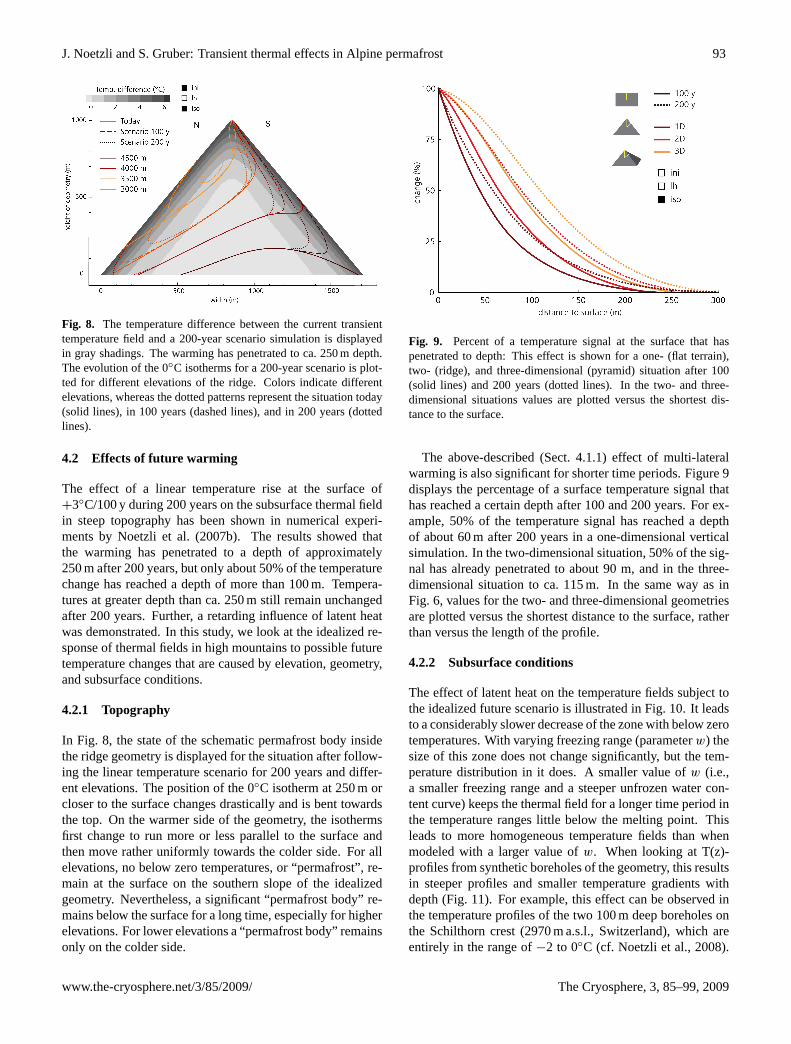
Fig. 9. Percent of a temperature signal at the surface that haspenetrated to depth: This effect is shown for a one- (flat terrain),two- (ridge), and three-dimensional (pyramid) situation after 100(solid lines) and 200 years (dotted lines). In the two- and three-dimensional situations values are plotted versus the shortest dis-tance to the surface.

The above-described (Sect. 4.1.1) effect of multi-lateralwarming is also significant for shorter time periods. Figure 9displays the percentage of a surface temperature signal thathas reached a certain depth after 100 and 200 years. For ex-ample, 50% of the temperature signal has reached a depthof about 60 m after 200 years in a one-dimensional verticalsimulation. In the two-dimensional situation, 50% of the sig-nal has already penetrated to about 90 m, and in the three-dimensional situation to ca. 115 m. In the same way as inFig. 6, values for the two- and three-dimensional geometriesare plotted versus the shortest distance to the surface, ratherthan versus the length of the profile.

4.2.2 Subsurface conditions

The effect of latent heat on the temperature fields subject tothe idealized future scenario is illustrated in Fig. 10. It leadsto a considerably slower decrease of the zone with below zerotemperatures. With varying freezing range (parameterw) thesize of this zone does not change significantly, but the tem-perature distribution in it does. A smaller value ofw (i.e.,a smaller freezing range and a steeper unfrozen water con-tent curve) keeps the thermal field for a longer time period inthe temperature ranges little below the melting point. Thisleads to more homogeneous temperature fields than whenmodeled with a larger value ofw. When looking at T(z)-profiles from synthetic boreholes of the geometry, this resultsin steeper profiles and smaller temperature gradients withdepth (Fig. 11). For example, this effect can be observed inthe temperature profiles of the two 100 m deep boreholes onthe Schilthorn crest (2970 m a.s.l., Switzerland), which areentirely in the range of−2 to 0◦C (cf. Noetzli et al., 2008).



Fig. 10. The permafrost body in a ridge calculated for a 200-yearscenario is displayed for simulations with and without consideringthe effects of latent heat and a porosity of 3%. Additionally, differ-ent values of the parameterw, which describes the unfrozen watercontent curve, have been considered. Black lines represent the mod-eled 0◦C isotherm, i.e., the remaining permafrost body; blue, red,and yellow lines the−1, −2, and−3◦C isotherms.

This points to subsurface material with a small freezing in-terval and a low value ofw. The observed higher ice-contentin the near-surface layer (cf. Sect. 4.1.2) can act as a bufferto temperature changes at the surface and further delay theshort-term reaction of the subsurface temperature field, whenlooking at time scales of the next 1–2 centuries (Fig. 11).

5 Application to the topographic setting of theMatterhorn

The Matterhorn (4478 m a.s.l.) in Switzerland is probablythe most prominent mountain peak in the European Alps. Itsdistinctive topography resembles a pyramid of about 1500 mheight with faces exposed to the four main orientations.Slope angles are>45◦C for most parts and only isolatedor thin patches of snow persist on the rock. With its ex-treme three-dimensional geometry, the Matterhorn consti-tutes a prime example for an application of the presentedmodeling approach to real topography. The application of themodeling procedure to the Matterhorn topography is seen asa step towards more natural conditions. Further, it is helpfulto intuitively understand the dimensions of changes shownin the results from idealized geometries. Based on the ex-perience gained with the previous experiments and the val-idations conducted (see Sect. 3.2), the modeling procedureallows to describe the principal pattern of the subsurface tem-perature and permafrost distribution inside the mountain andhow they may evolve in the future. However, results needto be interpreted with great care, especially where a consid-erable snow or glacier cover influences the ground temper-atures (cf. Sect. 6). For a detailed description and the re-quirement to accurately model subsurface temperatures, themodeling has to be calibrated and tested against measured

Fig. 11. T(z)-profiles of two synthetic boreholes vertical to theslope in the middle and the lower part of the North side of a ridge(cf. Fig. 10) illustrate the effect of latent heat and the freezing rangew. In addition, thick bright lines display the profile of a simulationwith a 20 m ice-rich layer at the surface.

data from the Matterhorn. Several measurement sites haverecently been instrumented and corresponding datasets willbe available soon. Temperature data are measured on theHornli Ridge (NE ridge: two 60 m boreholes close to theHornlihutte that are monitored within the PERMOS project(PERMOS, 2007), and extensive thermal and geotechnicalmeasurements at the 2003 rock fall scar within the projectPermaSense; Hasler et al., 2008) and the Lion Ridge (SWridge, Carell Hut, near surface temperature measurements inthe scope of the project PermaDataRock (Pogliotti, 2006).

Surface temperatures were modeled using climate time se-ries from the Corvatsch station in the Upper Engadine (datasource: MeteoSwiss), which is located on a summit in a cen-tral Alpine climate similar to the Matterhorn area (cf. Gru-ber et al., 2004b) at 3330 m a.s.l. This station was cho-sen because it was shown in previous studies (e.g., Suter,2002) that horizontal extrapolation of climate variables inmountain areas leads to smaller deviations than vertical ex-trapolation. Surface properties were used according to theprevious simulations (Table 1). The topography was takenfrom the 25 m DEM Level 2 by Swisstopo and the FE meshcontained approximately 55 000 elements. The lithology ofthe Matterhorn mainly consists of gneiss and granite of the



Fig. 12. North-south cross section of the Matterhorn (4478 m a.s.l.)and modeled subsurface temperature field for today (i.e., the meanof the period 1990–1999 AD). The temperature field was computedtransient, three-dimensional, isotropic, and with 3% subsurface icein the frozen parts. The black lines represent the 0◦C isotherms fortoday (solid line), in 100 years (dashed line), and in 200 years (dot-ted line). We assumed a linear warming scenario of+3◦C/100 y.DHM 25 reproduced by permission of swisstopo (BA091262).

east Alpine Dent-Blanche nappe. We set a thermal con-ductivity of 2.5 W m−1 K−1, a volumetric heat capacity of2.2×106 J m−3 K−1, a porosity of 3%, andw=2 (cf. Table 1).Boundary conditions and time steps were the same as in thesimulations presented above, and anisotropy was not consid-ered.

A north-south cross section through the resulting subsur-face temperature field for current conditions and the warm-ing scenario for 200 years is given in Fig. 12. The ex-treme pyramid-like geometry of the Matterhorn leads toa strongly three-dimensional subsurface temperature field,which is characterized by steeply inclined isotherms, a strongheat flux from the south to the north, and a smaller heat fluxfrom the east to the west face. For present-day conditionsand all the simplifications assumed for the simulation, theentire mountain is within permafrost, except for the lowerparts of the South side. Additionally considering the ideal-ized scenario, surface temperatures on nearly the entire Southside would be positive after 200 years. On the North side,the 0◦C isotherm at the surface would have risen to an el-evation of about 3500 m a.s.l. The calculated scenario indi-cates further that possibly substantial permafrost can remaina few decameters below the surface both, on the south andthe north side. Temperatures of the remaining sketched per-mafrost body are warming and the extent of so-called warmpermafrost (i.e., about−2 to 0◦C) would significantly in-crease in volume as well as in vertical extent (Fig. 13).

Fig. 13. Modeled temperature range of−2 to 0◦C in a north-southcross section of the Matterhorn for today (gray), in 100 years (lightred), and in 200 years (red). We assumed a linear warming scenarioof +3◦C/100 y. DHM 25 reproduced by permission of swisstopo(BA091262).

6 Discussion

With the numerical experiments based on simplified moun-tain topographies having idealized surface and subsurfaceconditions we analyzed the influence of combined transientand three-dimensional topography effects on the subsurfacetemperature field in mountain topographies. For the interpre-tation of the results, a number of uncertainties and limitationsof the modeling approach used are important and the simpli-fications made have to be kept in mind.

Instrumental records of climate parameters are typicallyavailable for the past ca. 100 years. Reconstructions of pre-industrial climate rely on proxy data and are subject to a greatnumber of uncertainties, which may be even larger than theinfluence a certain time period has on the subsurface tem-peratures. In general, climate reconstruction studies agreewell on the shape of the climate fluctuations, whereas theabsolute amplitude of the temperature variations ranges sig-nificantly (Esper et al., 2005). Further, we assumed thatchanges in GST closely follow air temperatures. Salzmannet al. (2007) demonstrated a considerable influence of topog-raphy on the reaction of surface temperatures in steep rockto changing atmospheric conditions. The dimensions of theGST changes, however, are not influenced, and in view ofthe above-mentioned uncertainties of the reconstructed am-plitudes of temperature variations, we consider this effect tobe less important for this study.

Much more important are changes in surface cover orsurface characteristics, which have been neglected in ouridealized simulations. This mainly concerns glacier cover-age and the influence of the snow cover. Haeberli (1983)points to higher temperatures at a glacier base than for rockexposed directly to the atmosphere during the past coldperiods and, hence, paleoclimatic effects below previously



glacier-covered areas are likely smaller than in rock directlyexposed to the atmosphere during the entire simulation pe-riod. This is likely important, for example, for the lower partsof the Matterhorn. In these parts, the temperature field shownin Figs. 12 and 13 has to be interpreted with great care andmay considerably deviate in nature. The negligence of thesnow cover is a further significant limitation of the model-ing approach: Snow cover affects the energy balance at theground surface by increasing albedo, consuming melt energy,and insulating the ground surface from atmospheric condi-tions. Snow that remains in steep bedrock can have both, acooling and a warming effect. For steep rock slopes, how-ever, these effects have not yet been investigated or quan-tified in detail and results from more gentle terrain cannotbe directly transferred to steeper areas (Gruber and Haeberli,2007). In view of applying the model to less inclined slopes,the influence of a snow cover will have to be included in themodel.

In terms of subsurface characteristics, errors induced byuncertain assumptions of thermal conductivity, heat capac-ity, and heat production increase with depth and length of thesimulation, whereas errors caused by uncertainties in sub-surface ice decrease. Information on the amount and freez-ing characteristics of subsurface ice in bedrock is required toimprove realistic modeling, but is still scarce. The joint in-terpretation of numerical model results with data from geo-physical monitoring (e.g., electrical resistivity tomography,ERT) has been successfully realized for a first case study ofthe Schilthorn crest in the Swiss Alps (Noetzli et al., 2008),and information gained in this way may help to improve therepresentation of the subsurface in the model.

Neglecting water circulation along the joint systems ofbedrock is another limitation of the approach used. Advec-tive heat transfer along clefts can contribute, for example,to subsurface heat transfer and lead to thaw corridors in per-mafrost, which substantially modify a purely conductive sys-tem (Gruber et al., 2004a; Gruber and Haeberli, 2007). Firstapplications of geophysical monitoring in solid rock walls re-cently identified thawed cleft systems influenced by movingwater (Krautblatter and Hauck, 2007). Process understand-ing of advective heat transfer processes in steep bedrock per-mafrost, however, is limited. But such processes are expectedto be important especially in the upper decameters.

We assumed a linear temperature rise of+3◦C in 100 y forthe calculations of the idealized response of the temperaturefields to future changes. An exponential temperature rise asgenerally proposed for climate change scenarios may slowdown the temperature changes calculated. Yet, the temper-ature increase assumed represents a calculated mean changein GST of Alpine bedrock (Salzmann et al., 2007) and is atthe lower range of the scenarios presented for air temperaturechange by IPCC (2007), where a double temperature raiseis not considered unrealistic or extreme for the Alps. Thegeneral pattern of a future temperature field that increasinglydeviates from steady state conditions and experiences major

changes in heat fluxes in the upper ca. 100–200 meters is notaffected by these uncertainties.

Because of its temperature range, the acceleration of sub-surface temperature changes through multi-lateral warming,and the virtual decoupling from the geothermal heat flux,bedrock permafrost in steep high mountain areas is partic-ularly sensitive to climate change. The simulations of pos-sible future subsurface temperatures with idealized moun-tain topographies point to long lasting and deep-reachingchanges in the subsurface thermal field. For all settings inthe experiments, only very little “permafrost” remains at thesurface on south-facing Alpine rock slopes in 200 years.Simulated 0◦C-isotherms are about to change to a surface-parallel course in the top parts of the mountain geometriesand then move rather uniformly towards the interior. In termsof temperature-related instabilities such a thawing and hori-zontally migrating permafrost table may be delicate: rockvolumes with temperatures close to the melting point, possi-bly containing critical ice-water-rock mixtures, increase andmay extend over large vertical distances up to entire moun-tain flanks.

Although our experiments were conducted for stronglyidealized conditions, the general pattern and the principal ef-fects shown in this paper can be transferred to real topogra-phies, but keeping in mind the above mentioned uncertaintiesand the fact that the situation in nature is more complicatedand additional processes may be important. For the idealizedand simplified present-day temperature field of the Matter-horn, for example, warm permafrost is indicated in the mid-dle part of the South side. In these areas, rock fall eventsactually have been observed in recent years (2003 and 2006).Looking at the scenario sketched, the zone having temper-ature little below the freezing point extends over the entiresouth face and, in addition, over large parts of the north face.Although the modeled temperature field can only be inter-preted as a very first approximation to the actual pattern inthe Matterhorn, this scenario describes how the surface tem-perature field may develop in view of future changes in at-mospheric conditions.

7 Conclusions and perspectives

The results of the simulations performed with idealized testcases of steep mountain topography lead to the followingconclusions:

The main variations in surface temperatures that influencepresent-day subsurface temperatures in Alpine permafrostare the last glacial period and the major temperature varia-tions in the past millennium.

Transient paleothermal effects caused by past climate vari-ations likely exist in the interior of high-mountain peaks.Modeled temperature depressions compared to stationaryconditions of present-day GST are in the range of−3◦C at



a distance of 500 m from the surface and for the idealizedmodel settings.

Transient effects likely become even more important fortemperature fields influenced by future warming. Model ex-periments point to temperature fields that are characterizedby long-term and deep reaching perturbations and by tem-perature patterns that strongly deviate from stationary condi-tions.

Two- and three-dimensional topography significantly ac-celerates the pace of a surface temperature signal enteringinto the subsurface. Together with the fast and unfiltered re-action of its surface to changes in atmospheric conditions andthe low ice content, this makes bedrock permafrost in highmountains particularly sensitive to changes.

For the time (20 kyr) and depth (ca. 500 m) scales consid-ered, the influence of latent heat on the temperature depres-sions caused by past GST variations is small in low porosityrock. In view of other sources of uncertainties (e.g., tem-perature reconstructions) this effect is not considered of ma-jor importance. In connection with possible future warming,however, latent heat effects considerably modify the pace ofpermafrost degradation and the pattern of the subsurface tem-perature field.

Temperatures of the schematic permafrost body in the ge-ometries are rising when applying the future scenarios, andthe extent of “warm permafrost” significantly increases involume as well as in vertical extent

The distribution and extent of temperatures little below themelting point in a warming subsurface temperature field issignificantly influenced by the freezing characteristics of thesubsurface material. A small freezing range leads to morehomogenous temperature fields and T(z) profiles with smalltemperature gradients.

The investigation of mountain permafrost by transientthree-dimensional modeling has only been used for a fewcase studies of real mountain topography so far. It bears po-tential for various applications that require knowledge of cur-rent and future thermal conditions of mountain permafrost,for instance, the reanalysis of the thermal conditions in rockfall starting zones located in permafrost areas, the improvedinterpretation of T(z) profiles measured in boreholes, andthe assessment of thermal conditions and their evolution inrock below infrastructure. The limitations and uncertaintiesdiscussed above call for improved knowledge of subsurfaceproperties in bedrock permafrost, as well as for enhancedvalidation and modeling practices. A promising approachmay be the combination of numerical modeling together withmeasurements and interpretation of field data. For example,the representation of the subsurface physical properties in themodel can be improved by incorporating subsurface informa-tion (e.g., geological structures, water/ice content) detectedby geophysical surveys. Further, process understanding andincorporation of advective heat transfer and snow remainingin steep rock will be important for a realistic modeling ofsubsurface temperature fields.

Acknowledgements.This study was supported by the SwissNational Science Foundation, as part of the NF 20-10796./1 project“Frozen rock walls and climate change: transient 3-dimensionalinvestigation of permafrost degradation”. Special thanks go to SvenFriedel for support with the COMSOL software and for providingan import routine for DEMs. Fruitful discussions with W. Haeberliand M. Hoelzle (University of Zurich, Switzerland) as well aswith T. Kohl (Geowatt AG, Zurich, Switzerland) were valuablycontributed to this study. Careful and constructive comments bythe two reviewers helped to improve the paper.

Edited by: A. Kaab

References

Anderson, D. M. and Tice, A. R.: Predicting unfrozen water con-tents in frozen soils from surface area measurements, HighwayResearch Record, 393, 12–18, 1972.

Beltrami, H.: On the relationship between ground temperature his-tories and meteorological records: A report on the Pomquet Sta-tion, Global Plaint. Change, 29, 327–348, 2001.

Beltrami, H., Ferguson, G., and Harris, R. N.: Long-term trackingof climate change by underground temperatures, Geophys. Res.Lett., 32, L19707, doi:10.1029/2005GL023714, 2005.

Beniston, M., Diaz, H. F., and Bradley, R. S.: Climatic change athigh elevation sites: An overview, Clim. Change, 36, 233–251,1997.

Beniston, M.: Mountain climates and climate change: An overviewof processes focusing on the European Alps, Pure Appl. Geo-phys., 162, 1587–1606, 2005.

Birch, F.: The effects of Pleistocene climatic variations upongeothermal gradients, Am. J. Sci., 246, 729–760, 1948.

Boehm, R., Auer, I., Brunetti, M., Maugeri, M., Nanni, T., andSchoener, W.: Regional temperature variability in the EuropeanAlps: 1760–1998 from homogenized instrumental time series,Int. J. Climatol., 21, 1779–1801, 2001.

Brown, R. J. E. and Pewe, T. L.: Distribution of permafrost in northamerica and its relationship to the environment, a review 1963–1973, 2nd International Conference on Permafrost. Proceedings,Yakutsk, USSR, 1973, 71–100, 1973.

Burga, C.: Vegetation history and paleoclimatology of the middleHolocene: Pollen analysis of Alpine peat bog sediments, cov-ered formerly by the Rutor Glacier, 2510 m (Aosta Valley, Italy),Global Ecol. Biogeogr., 1, 143–150, 1991.

Carslaw, H. S. and Jaeger, J. C.: Conduction of heat in solids,Oxford science publications, Clarendon Press, Oxford, 510 pp.,1959.

Casty, C., Wanner, H., Luterbacher, L., Esper, J., and Boehm, R.:Temperature and precipitation variability in the European Alpssince 1500, Int. J. Climatol., 25, 1855–1880, 2005.

Cermak, V. and Rybach, L.: Thermal conductivity and specific heatof minerals and rocks, in: Landolt-bornstein Zahlenwerte undFunktionen aus Naturwissenschaften und Technik, neue Serie,physikalische Eigenschaften der Gesteine (v/1a), edited by: An-geneister, G., Springer, Berlin, 305–343, 1982.

Crowley, T. J. and Lowery, T. S.: How warm was the MedievalWarm Period? Ambio, 29, 51–54, 2000.

Dahl-Jensen, D., Modegaard, K., Gundestrup, N., Clow, G. D.,Johnsen, S. J., Hansen, A. W., and Balling, N.: Past temperatures



directly from the Greenland Ice Sheet, Science, 282, 268–271,1998.

Davies, M. C. R., Hamza, O., and Harris, C.: The effect of rise inmean annual temperature on the stability of rock slopes contain-ing ice-filled discontinuities, Permafrost Periglac., 12, 137–144,2001.

Esper, J., Wilson, R. J. S., Frank, D. C., Moberg, A., Wanner, H.,and Luterbacher, J.: Climate: Past ranges and future changes,Quarternary Sci. Rev., 24, 2164–2166, 2005.

Goosse, H., Arzel, O., Luterbacher, J., Mann, M. E., Renssen, H.,Riedwyl, N., Timmermann, A., Xoplaki, E., and Wanner, H.: Theorigin of the European “Medieval Warm Period”, Clim. Past, 2,99–113, 2006,http://www.clim-past.net/2/99/2006/.

Gruber, S., Hoelzle, M., and Haeberli, W.: Permafrost thaw anddestabilization of Alpine rock walls in the hot summer of 2003,Geophys. Res. Lett., 31, L13504, doi:10.1029/2004GL0250051,2004a.

Gruber, S., Hoelzle, M., and Haeberli, W.: Rock wall temperaturesin the Alps: Modeling their topographic distribution and regionaldifferences, Permafrost Periglac., 15, 299–307, 2004b.

Gruber, S., King, L., Kohl, T., Herz, T., Haeberli, W., and Hoelzle,M.: Interpretation of geothermal profiles perturbed by topog-raphy: The Alpine permafrost boreholes at Stockhorn Plateau,Switzerland, Permafrost Periglac., 15, 349–357, 2004c.

Gruber, S.: Mountain permafrost: Transient spatial modelling,model verification and the use of remote sensing, PhD Thesis,Department of Geography, University of Zurich, Zurich, 2005.

Gruber, S., and Haeberli, W.: Permafrost in steep bedrockslopes and its temperature-related destabilization fol-lowing climate change, J. Geophys. Res., 112, F02S18,doi:10.1029/2006JF000547, 2007.

Haeberli, W.: Permafrost-glacier relationships in the Swiss Alps– today and in the past, 4th International Conference on Per-mafrost. Proceedings, Fairbanks, Alaska, 1983, 415–420,

Haeberli, W., Rellstab, W., and Harrison, W. D.: Geothermal effectsof 18 ka BP ice conditions in the Swiss Plateau, Ann. Glaciol., 5,56–60, 1984.

Haeberli, W.: Construction, environmental problems and naturalhazards in periglacial mountain belts, Permafrost Periglac., 3,111–124, 1992.

Haeberli, W., Wegmann, M., and Vonder Muhll, D.: Slope stabilityproblems related to glacier shrinkage and permafrost degradationin the Alps, Eclogae Geol. Helv., 90, 407–414, 1997.

Haeberli, W. and Beniston, M.: Climate change and its impacts onglaciers and permafrost in the Alps, in: Ambio – a journal of thehuman environment, edited by: Rapp, A., and Kessler, E., 4, TheRoyal Swedish Academy of Sciences, 258–265, 1998.

Harris, C., Davies, M. C. R., and Etzelmuller, B.: The assessmentof potential geotechnical hazards associated with mountain per-mafrost in a warming global climate, Permafrost Periglac., 12,145–156, 2001.

Hasler, A., Talzi, I., Beutel, J., Tschudin, C., and Gruber, S.: Wire-less sensor networks in permafrost research: Concept, require-ments, implementation, and challenges, 9th International Con-ference on Permafrost, Fairbanks, US, 669–674, 2008.

Hauck, C., Bach, M., and Hilbich, C.: A 4-phase model to quan-tify subsurface ice and water content in permafrost regions basedon geophysical datasets, 9th International Conference on Per-

mafrost, Fairbanks, US, 675–680, 2008.Huang, S., Pollak, H. N., and Shen, P. Y.: Temperature trends over

the last five centuries reconstructed from borehole temperatures,Nature, 403, 756–758, 2000.

Hughes, M. K., and Diaz, H. F.: Was there a “Medieval Warm Pe-riod”, and if so, where and when?, Clim. Change, 26, 109–142,1994.

IPCC: Climate change 2007: The physical science basis. Contribu-tion of working group I to the fourth assessment report of the In-tergovernmental Panel on Climate Change, edited by: Solomon,S., Qin, D., Manning, M., Chen, Z., Marquis, M., Averyt, K.B., Tignor, M., and Miller, H. L., Cambridge University Press,Cambridge, United Kingdom and New York, 996 pp., 2007.

Isaksen, K., Vonder Muhll, D., Gubler, H., Kohl, T., and Sollid,J. L.: Ground surface temperature reconstruction based on datafrom a deep borehole in permafrost at Janssonhaugen, Svalbard,Ann. Glaciol., 31, 287–294, 2000.

Isaksen, K., Sollid, J. L., Holmlund, P., and Harris, C.: Recentwarming of mountain permafrost in Svalbard and Scandinavia, J.Geophys. Res., 112, F02S04, doi:10.1029/2006JF000522, 2007.

Jones, P. D., Briffa, K. R., Barnett, T. P., and Tett, S. F. B.: High-resolution paleoclimatic records for the last millennium: Inter-pretation, integration, and comparison with general circulationmodel control-run temperatures, Holocene, 8, 455–471, 1998.

Jones, P. D. and Mann, M. E.: Climate over past millennia, Rev.Geophys., 42, RG2002, doi:2010.1025/2003RG000143, 2004.

Kohl, T.: Transient thermal effects at complex topographies,Tectonophysics, 306, 311–324, 1999.

Kohl, T., Signorelli, S., and Rybach, L.: Three-dimensional (3-D)thermal investigation below high Alpine topography, Phys. EarthPlaint. In., 126, 195–210, 2001.

Kohl, T. and Gruber, S.: Evidence of paleaotemperature signals inmountain permafrost areas, 8th International Conference on Per-mafrost, Extended Abstracts, Zurich, 83–84, 2003.

Krautblatter, M. and Hauck, C.: Electrical resistivity tomographymonitoring of permafrost in solid rock walls, J. Geophys. Res.,112, F02S20, doi:10.1029/2006JF000546, 2007.

Kukkonen, I. T. and Safanda, J.: Numerical modelling of permafrostin bedrock in northern Fennoscandia during the Holocene, Glob.Plaint. Change, 29, 259–273, 2001.

Lachenbruch, A. H. and Marshall, B. V.: Changing climate:Geothermal evidence from permafrost in the alaskan arctic, Sci-ence, 234, 689–696, 1986.

Luthi, M. and Funk, M.: Modelling heat flow in a cold, high-altitudeglacier: Interpretation of measurements from Colle Gnifetti,Swiss Alps, J. Glaciol., 47, 314–324, 2001.

Lunardini, V. J.: Climatic warming and the degradation of warmpermafrost, Permafrost Periglac., 7, 311–320, 1996.

Luterbacher, J., Dietrich, D., Xoplaxi, E., Grosjean, M., and Wan-ner, H.: European seasonal and annual temperature variability,trends and extremes since 1500, Science, 303, 1499–1503, 2004.

Medici, F. and Rybach, L.: Geothermal map of Switzerland1995 (heat flow density), Geophysique 30, Schweizerische Geo-physikalische Kommission, 1995.

Mottaghy, D. and Rath, V.: Latent heat effects in subsurface heattransport modeling and their impact on paleotemperature recon-structions, Geophys. J. Int., 164, 236–245, 2006.

Noetzli, J.: Modeling transient three-dimensional temperature fieldsin mountain permafrost, PhD Thesis, Department of Geography,


http://www.clim-past.net/2/99/2006/


University of Zurich, Zurich, 150 pp., 2008.Noetzli, J., Hoelzle, M., and Haeberli, W.: Mountain permafrost

and recent Alpine rock-fall events: A GIS-based approach todetermine critical factors, 8th International Conference on Per-mafrost, Proceedings, Zurich, 827–832, 2003.

Noetzli, J., Gruber, S., and Friedel, S.: Modeling transient per-mafrost temperatures below steep Alpine topography, COMSOLUser Conference, Grenoble, 139–143, 2007a.

Noetzli, J., Gruber, S., Kohl, T., Salzmann, N., and Haeberli, W.:Three-dimensional distribution and evolution of permafrost tem-peratures in idealized high-mountain topography, J. Geophys.Res., 112, F02S13, doi:10.1029/2006JF000545, 2007b.

Noetzli, J., Hilbich, C., Hauck, C., Hoelzle, M., and Gruber, S.:Comparison of simulated 2D temperature profiles with time-lapse electrical resistivity data at the Schilthorn crest, Switzer-land., 9th International Conference on Permafrost, Fairbanks,US, 2008, 1293–1298.

Patzelt, G.: Neue Ergebnisse der Spat- und Postglazialforschu-ung in Tirol, in: Jahresbericht,Osterreichische GeographischeGesellschaft, Zweigverein Innsbruck, 11–18, 1987.

PERMOS: Permafrost in Switzerland 2002/2003 and 2003/2004,Glaciological report (Permafrost) no. 4/5 of the CryosphericCommission of the Swiss Academy of Sciences (SCNAT) andDepartment of Geography, University of Zurich, edited by: Von-der Muehll, D., Noetzli, J., Roer, I., Makowski, K., and Delaloye,R., 104 pp., 2007.

Petit, J. R., Jouzel, J., Raynnaud, D., Barkov, N. I., Barnola, J.-M.,Basile, I., Bender, M., Chappellaz, J., Davis, M., Delaygue, G.,Delmotte, M., Kotlyakov, V. M., Legrand, M., Lipenkov, V. Y.,Lorius, C., Pepin, L., Ritz, C., Saltzman, E., and Stievenard, M.:Climate and atmospheric history of the past 420 000 years fromthe Vostok ice core, Antarctica, Nature, 399, 429–436, 1999.

Pfister, C.: Wetternachhersage, Haupt, Bern, 304 pp., 1999.Pogliotti, P.: Analisi morfostrutturale e caratterizzazione termica

di ammassi rocciosi recentemente deglaciati. MSc Thesis, HeartScience Department, University of Turin, Turin, 191 pp., 2006.

Pollak, H. N., Huang, S., and Shen, P. Y.: Climate change recordin subsurface temperatures: A global perspective, Science, 282,279–281, 1998.

Pollak, H. N. and Huang, J.: Climate reconstruction from subsur-face temperatures, Ann. Rev. Earth Plaint. Sci., 28, 339–365,2000.

Romanovsky, V. E. and Osterkamp, T. E.: Effects of unfrozen wa-ter on heat and mass transport processes in the active layer andpermafrost, Permafrost Periglac., 11, 219–239, 2000.

Romanovsky, V. E., Gruber, S., Instanes, A., Jin, H., Marchenko,S. S., Smith, S. L., Trombotto, D., and Walter, K. M.: Frozenground, in: Global outlook for ice and snow, edited by: UNEP,UNEP/GRID-Arendal, Norway, 182–200, 2007.

Safanda, J.: Ground surface temperature as a function of slope angleand slope orientation and its effect on the subsurface temperaturefield, Tectonophysics, 306, 367–375, 1999.

Safanda, J. and Rajver, D.: Signature of the last ice age inthe present subsurface temperatures in the Czech Republic andSlovenia, Glob. Plaint. Change, 29, 241–257, 2001.

Salzmann, N., Noetzli, J., Gruber, S., Hauck, C., and Haeberli, W.:RCM-based ground temperature scenarios in high-mountain to-pography and their uncertainty ranges, J. Geophys. Res., 112,F02S12, doi:10.1029/2006JF000527, 2007.

Scherler, M.: Messung und Modellierung konvektiverWarmetransportprozesse in der Auftauschicht von Gebirgsper-mafrost am Beispiel des Schilthorns, Department of Geography,University of Zurich, Zurich, 94 pp., 2006.

Schoen, J.: Petrophysik, Ferdinand Enke, Stuttgart, 1983.Stocker-Mittaz, C.: Permafrost distribution modeling based on en-

ergy balance data. PhD-Thesis, Department of Geography, Uni-versity of Zurich, Zurich, 122 pp., 2002.

Suter, S.: Cold firn and ice in the monte rosa and mont blanc areas:spatial occurrence, surface energy balance and climatic evidence,172, Versuchsanstalt fur Wasserbau, Hydrologie und Glaziologieder ETH Zurich, ETH Zurich, Zurich, 188 pp., 2002.

Von Rudloff, H.: Das Klima – Entwicklung in den letzten Jahrhun-derten im mitteleuropaischen Raume (mit einem Ruckblick aufdie postglaziale Periode), in: Das Klima – Analysen und Mod-elle, Geschichte und Zukunft, edited by: Oeschger, H., Messerli,B., and Silvar, M., Springer, Berlin, 125–148, 1980.

Washburn, A. L.: Geocryology – a survey of periglacial processesand environments, edited by: Quartenary Research Center, U. o.W., Edward Arnold Ltd., London, 406 pp., 1979.

Wegmann, M.: Frostdynamik in hochAlpinen Felswanden amBeispiel der Region Jungfraujoch-Aletsch, 161, Versuchsanstaltfur Wasserbau, Hydrologie und Glaziologie der ETH Zurich,ETH Zurich, Zurich, 143 pp., 1998.

Wegmann, M., Gudmundsson, G. H., and Haeberli, W.: Permafrostchanges in rock walls and the retreat of Alpine glaciers: A ther-mal modelling approach, Permafrost Periglac., 9, 23–33, 1998.

Williams, P. J. and Smith, M. W.: The frozen earth, 1 ed., Studiesin polar research, Cambridge University Press, Cambridge, 306pp., 1989.


transient thermal effects in alpine permafrost - the cryosphere

Documents