Transit-Oriented Development Deployment Strategies to Maximize Integrated Transportation and Land Use Life Cycle Greenhouse Gas Reductions

Mikhail Chester Arizona State University, mchester@asu.edu Dwarakanath Ravikumar Arizona State University, dtriplic@asu.edu

Abstract. Urban sustainability decision makers should incorporate time-based impacts of greenhouse gas emissions with life cycle assessment to improve climate change mitigation strategies. As cities develop strategies that move development closer to transit systems and encourage households to live in lower energy configurations, new methods are needed for understanding how upfront emissions of greenhouse gases produce long run radiative forcing impacts. Using an existing assessment of the development potential around Phoenix’s new light rail system, a framework is developed for deploying higher density, lower energy use, and more transit-friendly households near light rail given financing constraints. The case study compares development around transit stations in Phoenix against continued outward growth of single family homes. Using this case study, the significance of greenhouse gas (GHG) radiative forcing discounting is assessed. The radiative forcing benefits of different levels of financing aggressiveness are shown. A comparison of payback on upfront construction impacts for long run benefits is developed between the GHG accounting approach and the radiative forcing approach, the latter of which accounts for time-based GHG impacts. The results show that the radiative forcing approach puts more weight on upfront construction impacts and pushes the payback on initial investments out further than when GHG accounting is used. It is possible to reduce this payback time by providing a larger upfront financing resource. Ultimately, policy and decision makers should use radiative forcing measures over GHG measures because it will provide a measure that discounts GHG emissions at different times to a normalized unit.

Introduction. Many cities have experienced rapid and unconstrained growth in the latter half of the twentieth century and as energy and greenhouse gas concerns receive increasing attention, there is growing interest in developing strategies that concentrate future growth towards urban centers. This inward growth has the potential to reduce the energy and greenhouse gas (GHG) intensity of new dwelling units through the use of higher density building designs. It could also reduce transportation energy use and GHG emissions by providing opportunity for future residents to use transit and also reduce their household automobile travel by more centrally locating homes. Kimball et al. (2013) developed an integrated transportation and land use life cycle assessment (ITLU-LCA) of Phoenix’s light rail system to determine energy, greenhouse gas, respiratory, and smog impact long-run changes in the region from land development around the transit line. Kimball et al. (2013) determined that in the most aggressive development outcome, where vacant and dedicated surface lots within one-half mile of stations are turned into multi-family apartment or condominium units, the Phoenix metro area would avoid roughly 11 Tg CO2e over 60 years.

Proceedings of the International Symposium on Sustainable Systems and Technologies (ISSN 2329-9169) is published annually by the Sustainable Conoscente Network. Melissa Bilec and Jun-ki Choi, co-editors. ISSSTNetwork@gmail.com.

Copyright © 2013 by Mikhail Chester and Dwarakanath Ravikumar. Licensed under CC-BY 3.0.

Cite as:Transit-Oriented Development Deployment Strategies to Maximize Integrated Transportation and Land Use Life Cycle Greenhouse Gas Reductions. Proc. ISSST, Mikhail Chester, Dwarakanath Ravikumar. http://dx.doi.org/10.6084/m9.figshare.805094. v1 (2013)

Page 2 of 10 Copyright © 2013 by Mikhail Chester and Dwarakanath Ravikumar

Comparing to current growth patterns that favor auto-dominated single family home development, the per dwelling unit savings are as large as 500 Mg CO2e. This is the result of lower home energy footprints and reduced automobile travel which leads to additional reductions in GHG emissions from reduced electricity generation primary fuel processing and the delaying of new automobile manufacturing. The LCA also shows that these transit oriented developments (TODs) have higher building construction footprints that enable these long run GHG savings. Given these TOD dwelling unit savings, there exists an opportunity to explore the development of strategies that deploy higher density dwelling units that are constrained by investment capital. If a city were to establish policies that promoted TODs, how quickly and in what form (e.g., density, building types) should buildings be deployed around transit stations to maximize GHG reductions as quickly as possible?

Densification of land around existing transit lines has the potential to produce GHG emissions reductions across both transportation and land use activities, and development can be scheduled across space and time to maximize reductions. Most modern US cities have invested in public transit infrastructure often with the goal of providing coverage to meet the mobility needs of population subgroups that cannot rely on private automobile travel. These transportation infrastructure are deployed and operated without comprehensive planning policies that affect surround land use. One such example of this is the Phoenix metro area’s light rail system. For two decades, the transit agency fought to secure funding for the line and there was little support for comprehensive policies that would also redevelop land around future stations. In 2008 the light rail line was completed and began operating. While well utilized, there are 730 acres of vacant land and dedicated surface parking lots within one-half mile (the generally accepted maximum walking distance to a bus or train station) of stations (Kimball et al., 2013). This land could accommodate 21,686 higher density dwelling units and potentially avoid the low density outward single family home sprawl that is typical of Phoenix. While these higher density dwelling units can produce GHG savings, the ITLU-LCA framework shows that upfront emissions investments are needed (i.e., the release of more GHG emissions for higher density dwelling units due to heavier use of materials, particularly concrete) to produce long run savings. Furthermore, behavioral changes that result in decreased automobile travel and decreased home energy use are more likely the closer residents are to the transit stations. Despite literature that suggests that TODs can be successful within one-half mile of stations, it is reasonable to assume that the greatest benefits will come from residents that live closest to the stations. Development of these 730 acres should prioritize land closest to the stations (e.g, within one-quarter mile) but must also be sensitive to the upfront emissions that are released from higher density home construction.

Goals. A framework is needed for managing the densification of neighborhoods that is sensitive to space and time, acknowledges financing constraints, and recognizes the time-based impacts of GHG emissions. Carbon emitted to the atmosphere is reabsorbed by the oceans and terrestrial environments at a nonlinear rate (Kendall et al., 2009) and urban GHG reduction goals should be sensitive to this dynamic. Effectively, carbon emitted during the early stages of transit-oriented development has more potential for radiative forcing in a fixed time period that is relevant to a policy goal than carbon emitted later on (O’Hare et al., 2009). A TOD deployment framework is developed using the land around Phoenix light rail as a case study. The ITLU-LCA results for Phoenix TODs from Kimball et al. (2013) are used. Assuming a financing schedule, an optimal deployment framework is determined that reports the number of multi-family and single family homes that the metropolitan region should construct each year within one-quarter and one-half mile of light rail stations to maximize both GHG emissions reductions as well as Cumulative Radiative Forcing (CRF), the latter of which considers the disproportionate upfront impacts of carbon emissions. By changing the total financial investment in densification in the

Page 3 of 10 Copyright © 2013 by Mikhail Chester and Dwarakanath Ravikumar

long-run, the changes in the construction schedule are explored. Lastly, the deployment framework will be used to assess benefits and costs (in both climate and economic) and determine who in a city is responsible for these effects.

Investigative Method. This project compares the impacts of CO2 emissions from business as usual (BAU) and TOD scenarios. An assessment of 21,686 new dwelling units is completed to satisfy some of Phoenix’s expected population growth. These dwelling units are based on the maximum number of dwelling units that can be constructed within one-half mile of Phoenix’s new light rail station, as determined by Kimball et al. (2013). If these TOD dwelling units are not constructed near light rail, then it is assumed that an equivalent number of dwelling units will need to be constructed in a BAU scenario in typical outgrowing Phoenix design, with its auto-dominated travel. In the TOD scenario, Kimball et al. (2013) estimate that 20,800 multi-family dwelling units can be constructed within a one-half mile radius of light rail transit (LRT) stations plus an additional 886 single family (SF) homes (the latter where parcels are too small for large multi-family apartment buildings). These TOD dwelling units (DU) will be closer to light rail and will i) have an opportunity to shift a fraction of their household trips to light rail and ii) live in smaller dwelling units (on average 1,000 ft2) therefore requiring less energy for lighting and HVAC. The shifting of household trips from cars to light rail results in fewer household yearly personal vehicle miles of travel thus increasing their car lifetime and ultimately delaying the manufacturing of a new vehicle. However, these new TODs result in a demand for additional light rail service and therefore new trains. In the BAU scenario, 21,686 single family homes are constructed in outlying areas where households will only be able to travel by automobile and homes are larger (on average 1,600 ft2). A comparison of these scenarios is shown in Table 1.

Table 1. DU Construction/Maintenance and Transportation details for TOD and BAU scenarios.

BAU TOD

SF Dwelling Units 21,686 886

MF Dwelling Units - 20,800

Car Life (Years) 4 9

Years in which LRTs are Manufactured - Year 1 and 30

Life Cycle Processes Building and Car Operations Building, Car, and LRT operations

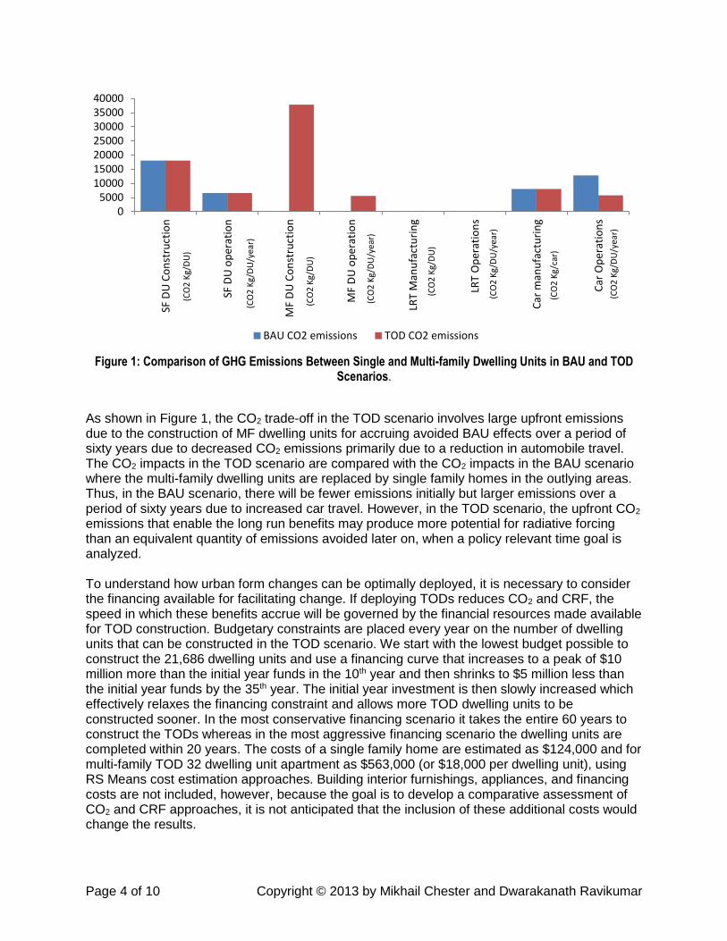
The CO2 emissions associated with the BAU and the TOD scenario are shown in Figure 1 and are from Kimball et al. (2013). The CO2 emissions from constructing a multi-family dwelling unit (38 Mg of CO2 /DU) are twice that of a single family home (18 Mg of CO2 /DU). A multi-family apartment building with 32 dwelling units was modeled and the use of concrete for these structures over wood in a single family home results in the higher per dwelling unit emissions for TOD structures. The CO2 emissions from car usage is 5.7 Mg/DU/year and 13 Mg/DU/year for the TOD and BAU scenarios respectively. Moreover, once constructed, the CO2 emissions of associated with electricity generation for TOD dwelling unit operations are around 15% less (5.5 Mg of CO2 /DU/year) than that of a single family home in the BAU scenario (6.5 Mg of CO2/DU/year). The CO2 emissions from LRT manufacturing and use in the TOD scenario are small compared to the other life cycle processes.

Page 4 of 10 Copyright © 2013 by Mikhail Chester and Dwarakanath Ravikumar

Figure 1: Comparison of GHG Emissions Between Single and Multi-family Dwelling Units in BAU and TOD Scenarios.

As shown in Figure 1, the CO2 trade-off in the TOD scenario involves large upfront emissions due to the construction of MF dwelling units for accruing avoided BAU effects over a period of sixty years due to decreased CO2 emissions primarily due to a reduction in automobile travel. The CO2 impacts in the TOD scenario are compared with the CO2 impacts in the BAU scenario where the multi-family dwelling units are replaced by single family homes in the outlying areas. Thus, in the BAU scenario, there will be fewer emissions initially but larger emissions over a period of sixty years due to increased car travel. However, in the TOD scenario, the upfront CO2 emissions that enable the long run benefits may produce more potential for radiative forcing than an equivalent quantity of emissions avoided later on, when a policy relevant time goal is analyzed.

To understand how urban form changes can be optimally deployed, it is necessary to consider the financing available for facilitating change. If deploying TODs reduces CO2 and CRF, the speed in which these benefits accrue will be governed by the financial resources made available for TOD construction. Budgetary constraints are placed every year on the number of dwelling units that can be constructed in the TOD scenario. We start with the lowest budget possible to construct the 21,686 dwelling units and use a financing curve that increases to a peak of $10 million more than the initial year funds in the 10th year and then shrinks to $5 million less than the initial year funds by the 35th year. The initial year investment is then slowly increased which effectively relaxes the financing constraint and allows more TOD dwelling units to be constructed sooner. In the most conservative financing scenario it takes the entire 60 years to construct the TODs whereas in the most aggressive financing scenario the dwelling units are completed within 20 years. The costs of a single family home are estimated as $124,000 and for multi-family TOD 32 dwelling unit apartment as $563,000 (or $18,000 per dwelling unit), using RS Means cost estimation approaches. Building interior furnishings, appliances, and financing costs are not included, however, because the goal is to develop a comparative assessment of CO2 and CRF approaches, it is not anticipated that the inclusion of these additional costs would change the results.

05000

10000150002000025000300003500040000

SF D

U C

on

stru

ctio

n

SF D

U o

per

atio

n

MF

DU

Co

nst

ruct

ion

MF

DU

op

erat

ion

LRT

Man

ufa

ctu

rin

g

LRT

Op

erat

ion

s

Car

man

ufa

ctu

rin

g

Car

Op

era

tio

ns

BAU CO2 emissions TOD CO2 emissions

(CO

2 K

g/D

U)

(CO

2 K

g/D

U/y

ear)

(CO

2 K

g/D

U)

(CO

2 K

g/D

U/y

ear)

(CO

2 K

g/D

U)

(CO

2 K

g/D

U/y

ear)

(CO

2 K

g/ca

r)

(CO

2 K

g/D

U/y

ear)

Page 5 of 10 Copyright © 2013 by Mikhail Chester and Dwarakanath Ravikumar

In addition to financing constraints there are locational constraints that ensure that only after the construction of all quarter-mile dwelling units are complete can construction start between one-quarter and one-half mile of stations. This is driven by the rationale that CO2 reductions from the behavioral changes are more likely to occur within one-quarter mile of light rail stations than further away.

Bern’s Decay Equation and CRF. Bern's decay equation is used to model the decay of CO2 released into the atmosphere when buildings and vehicles are built, manufactured and operated over 60 years in the BAU and TOD scenarios. The CRF impacts of these CO2 emissions are sensitive to the time at which these emissions occur. The CRF approach will account for the time at which the emission occurs and will not aggregate the impacts to a single point of time at the start or end of the policy time frame.

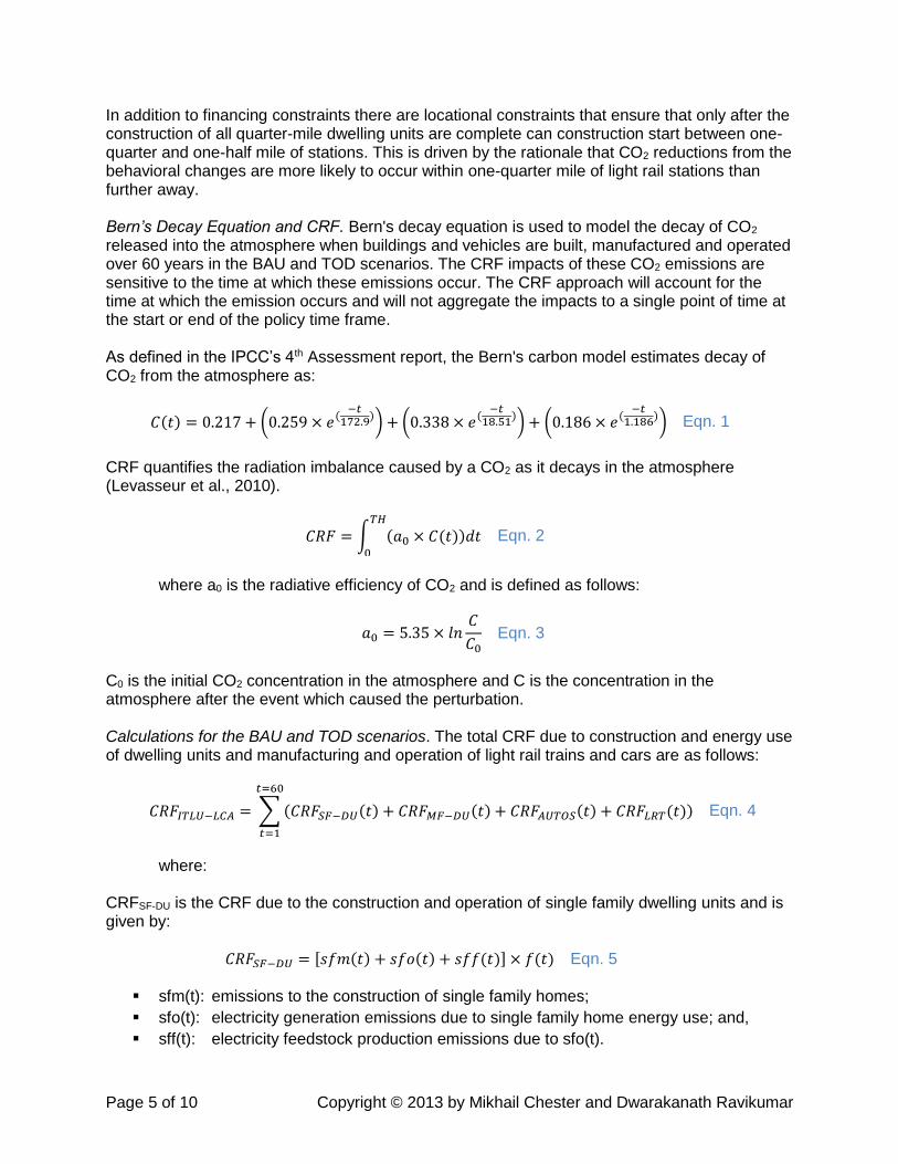
As defined in the IPCC’s 4th Assessment report, the Bern's carbon model estimates decay of CO2 from the atmosphere as:

𝐶(𝑡) = 0.217 + (0.259 × 𝑒(−𝑡

172.9)) + (0.338 × 𝑒(

−𝑡18.51

)) + (0.186 × 𝑒(−𝑡

1.186)) Eqn. 1

CRF quantifies the radiation imbalance caused by a CO2 as it decays in the atmosphere (Levasseur et al., 2010).

𝐶𝑅𝐹 = ∫ (𝑎0 × 𝐶(𝑡))𝑑𝑡𝑇𝐻

0

Eqn. 2

where a0 is the radiative efficiency of CO2 and is defined as follows:

𝑎0 = 5.35 × 𝑙𝑛𝐶

𝐶0Eqn. 3

C0 is the initial CO2 concentration in the atmosphere and C is the concentration in the atmosphere after the event which caused the perturbation.

Calculations for the BAU and TOD scenarios. The total CRF due to construction and energy use of dwelling units and manufacturing and operation of light rail trains and cars are as follows:

𝐶𝑅𝐹𝐼𝑇𝐿𝑈−𝐿𝐶𝐴 = ∑(𝐶𝑅𝐹𝑆𝐹−𝐷𝑈(𝑡) + 𝐶𝑅𝐹𝑀𝐹−𝐷𝑈(𝑡) + 𝐶𝑅𝐹𝐴𝑈𝑇𝑂𝑆(𝑡) + 𝐶𝑅𝐹𝐿𝑅𝑇(𝑡))

𝑡=60

𝑡=1

Eqn. 4

where:

CRFSF-DU is the CRF due to the construction and operation of single family dwelling units and is given by:

𝐶𝑅𝐹𝑆𝐹−𝐷𝑈 = [𝑠𝑓𝑚(𝑡) + 𝑠𝑓𝑜(𝑡) + 𝑠𝑓𝑓(𝑡)] × 𝑓(𝑡) Eqn. 5

sfm(t): emissions to the construction of single family homes;

sfo(t): electricity generation emissions due to single family home energy use; and,

sff(t): electricity feedstock production emissions due to sfo(t).

Page 6 of 10 Copyright © 2013 by Mikhail Chester and Dwarakanath Ravikumar

CRFMF-DU is the CRF due to the construction and operation of multi-family dwelling units and is given by:

𝐶𝑅𝐹𝑀𝐹−𝐷𝑈 = [𝑚𝑓𝑚(𝑡) + 𝑚𝑓𝑜(𝑡) + 𝑚𝑓𝑓(𝑡)] × 𝑓(𝑡) Eqn. 6

mfm(t): emissions to the construction of multi-family dwelling units;

mfo(t): electricity generation emissions due to multi-family dwelling unit energy use; and,

mff(t): electricity feedstock production emissions due to mfo(t).

CRFAUTO is the CRF due to the manufacturing and operation of cars and is given by:

𝐶𝑅𝐹𝐴𝑈𝑇𝑂𝑆 = [𝑎𝑢𝑚(𝑡) + 𝑎𝑢𝑜(𝑡) + 𝑎𝑢𝑓(𝑡)] × 𝑓(𝑡) Eqn. 7

aum(t): emissions due to manufacturing cars for the first time and repeat purchases at

end-of-life. New cars are purchased once every 4 years in business-as-usual scenarios

and every 9 years in the TOD scenarios;

auo(t): fuel consumption emissions due to car operations; and,

auf(t): feedstock consumption emissions due to auo(t).

CRFLRT is the CRF due to the manufacturing and operation of light rail trains and is given by:

𝐶𝑅𝐹𝐿𝑅𝑇 = [𝑙𝑟𝑚(𝑡) + 𝑙𝑟𝑜(𝑡) + 𝑙𝑟𝑓(𝑡)] × 𝑓(𝑡) Eqn. 8

lrm(t): emissions due to manufacturing LRT in year 1 and year 30 only;

lro(t): electricity generation emissions due to the operation of trains; and,

lrf(t): electricity feedstock emissions due to lro(t).

f(t) is given by:

𝑓(𝑡) = 𝑎𝐶 × [(𝑎0 × 𝑛) + (𝑎1 × 𝑐ℎ𝑖1 × (1 − 𝑒−𝑛−𝑡+1𝑐ℎ𝑖1 )) + (𝑎2 × 𝑐ℎ𝑖2 × (1 − 𝑒

−𝑛−𝑡+1𝑐ℎ𝑖2 ))

+ (𝑎3 × 𝑐ℎ𝑖3 × (1 − 𝑒−𝑛−𝑡+1𝑐ℎ𝑖3 ))]

Eqn. 9

where:

n is the number of years, which equals 60 in this study, and,

ac, ao, a1, a2, a3, chi1, chi2, chi3 are constants in Bern's decay model.

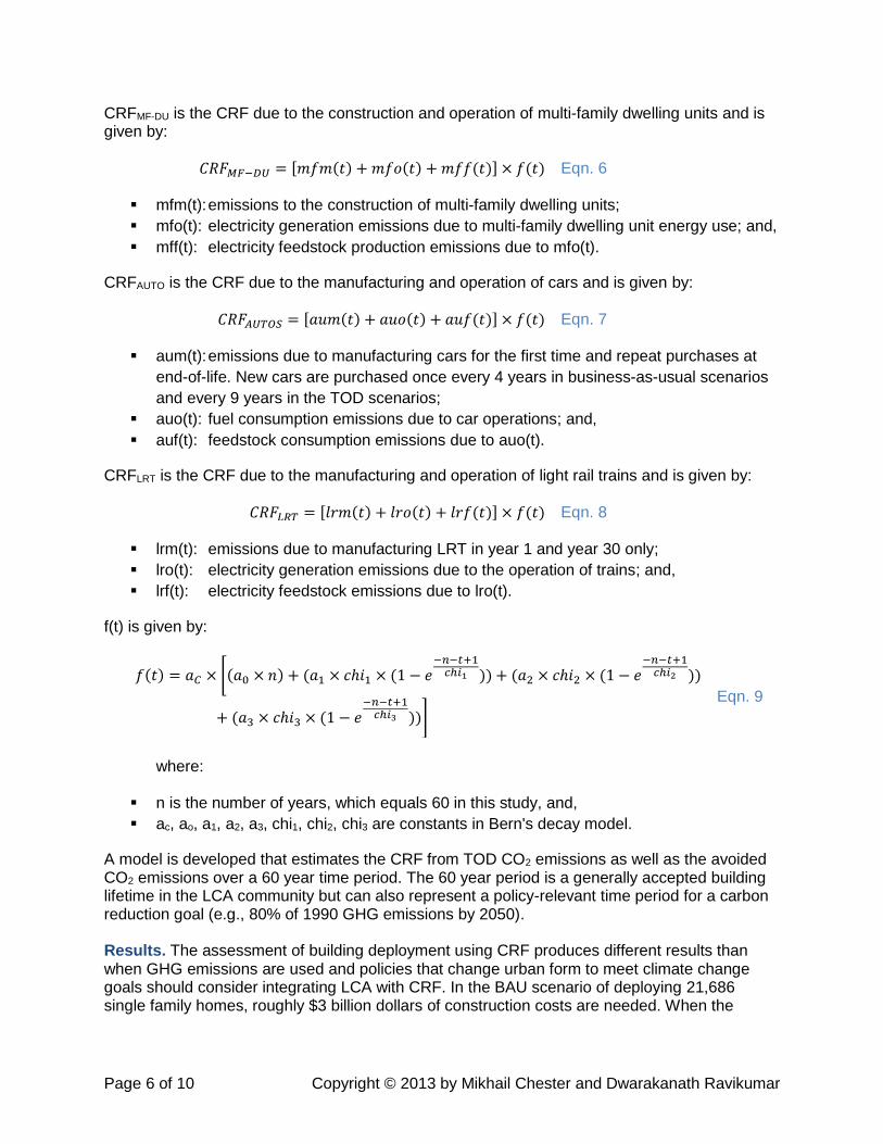
A model is developed that estimates the CRF from TOD CO2 emissions as well as the avoided CO2 emissions over a 60 year time period. The 60 year period is a generally accepted building lifetime in the LCA community but can also represent a policy-relevant time period for a carbon reduction goal (e.g., 80% of 1990 GHG emissions by 2050).

Results. The assessment of building deployment using CRF produces different results than when GHG emissions are used and policies that change urban form to meet climate change goals should consider integrating LCA with CRF. In the BAU scenario of deploying 21,686 single family homes, roughly $3 billion dollars of construction costs are needed. When the

Page 7 of 10 Copyright © 2013 by Mikhail Chester and Dwarakanath Ravikumar

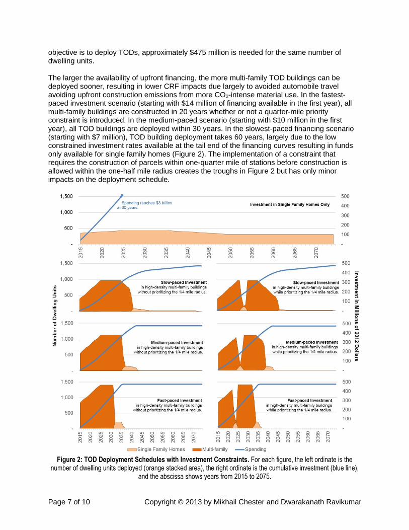
objective is to deploy TODs, approximately $475 million is needed for the same number of dwelling units. The larger the availability of upfront financing, the more multi-family TOD buildings can be deployed sooner, resulting in lower CRF impacts due largely to avoided automobile travel avoiding upfront construction emissions from more CO2-intense material use. In the fastest-paced investment scenario (starting with $14 million of financing available in the first year), all multi-family buildings are constructed in 20 years whether or not a quarter-mile priority constraint is introduced. In the medium-paced scenario (starting with $10 million in the first year), all TOD buildings are deployed within 30 years. In the slowest-paced financing scenario (starting with $7 million), TOD building deployment takes 60 years, largely due to the low constrained investment rates available at the tail end of the financing curves resulting in funds only available for single family homes (Figure 2). The implementation of a constraint that requires the construction of parcels within one-quarter mile of stations before construction is allowed within the one-half mile radius creates the troughs in Figure 2 but has only minor impacts on the deployment schedule.

Figure 2: TOD Deployment Schedules with Investment Constraints. For each figure, the left ordinate is the

number of dwelling units deployed (orange stacked area), the right ordinate is the cumulative investment (blue line), and the abscissa shows years from 2015 to 2075.

Page 8 of 10 Copyright © 2013 by Mikhail Chester and Dwarakanath Ravikumar

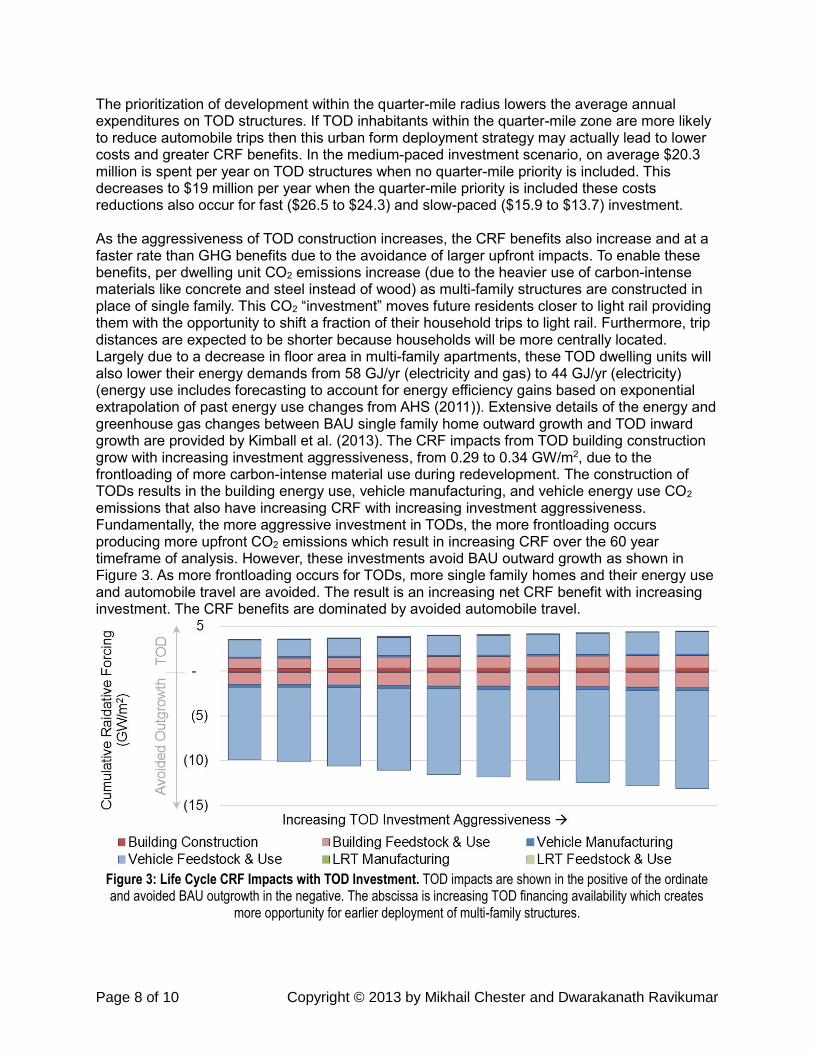
The prioritization of development within the quarter-mile radius lowers the average annual expenditures on TOD structures. If TOD inhabitants within the quarter-mile zone are more likely to reduce automobile trips then this urban form deployment strategy may actually lead to lower costs and greater CRF benefits. In the medium-paced investment scenario, on average $20.3 million is spent per year on TOD structures when no quarter-mile priority is included. This decreases to $19 million per year when the quarter-mile priority is included these costs reductions also occur for fast ($26.5 to $24.3) and slow-paced ($15.9 to $13.7) investment. As the aggressiveness of TOD construction increases, the CRF benefits also increase and at a faster rate than GHG benefits due to the avoidance of larger upfront impacts. To enable these benefits, per dwelling unit CO2 emissions increase (due to the heavier use of carbon-intense materials like concrete and steel instead of wood) as multi-family structures are constructed in place of single family. This CO2 “investment” moves future residents closer to light rail providing them with the opportunity to shift a fraction of their household trips to light rail. Furthermore, trip distances are expected to be shorter because households will be more centrally located. Largely due to a decrease in floor area in multi-family apartments, these TOD dwelling units will also lower their energy demands from 58 GJ/yr (electricity and gas) to 44 GJ/yr (electricity) (energy use includes forecasting to account for energy efficiency gains based on exponential extrapolation of past energy use changes from AHS (2011)). Extensive details of the energy and greenhouse gas changes between BAU single family home outward growth and TOD inward growth are provided by Kimball et al. (2013). The CRF impacts from TOD building construction grow with increasing investment aggressiveness, from 0.29 to 0.34 GW/m2, due to the frontloading of more carbon-intense material use during redevelopment. The construction of TODs results in the building energy use, vehicle manufacturing, and vehicle energy use CO2 emissions that also have increasing CRF with increasing investment aggressiveness. Fundamentally, the more aggressive investment in TODs, the more frontloading occurs producing more upfront CO2 emissions which result in increasing CRF over the 60 year timeframe of analysis. However, these investments avoid BAU outward growth as shown in Figure 3. As more frontloading occurs for TODs, more single family homes and their energy use and automobile travel are avoided. The result is an increasing net CRF benefit with increasing investment. The CRF benefits are dominated by avoided automobile travel.

Figure 3: Life Cycle CRF Impacts with TOD Investment. TOD impacts are shown in the positive of the ordinate and avoided BAU outgrowth in the negative. The abscissa is increasing TOD financing availability which creates

more opportunity for earlier deployment of multi-family structures.

Page 9 of 10 Copyright © 2013 by Mikhail Chester and Dwarakanath Ravikumar

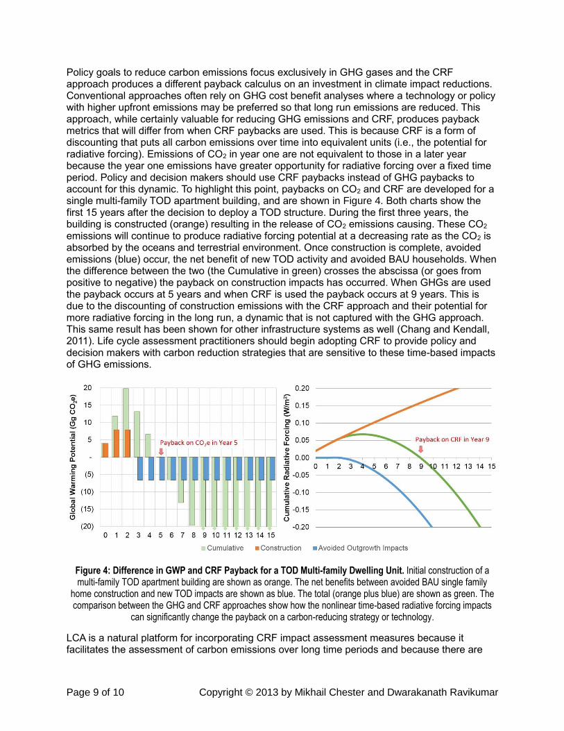
Policy goals to reduce carbon emissions focus exclusively in GHG gases and the CRF approach produces a different payback calculus on an investment in climate impact reductions. Conventional approaches often rely on GHG cost benefit analyses where a technology or policy with higher upfront emissions may be preferred so that long run emissions are reduced. This approach, while certainly valuable for reducing GHG emissions and CRF, produces payback metrics that will differ from when CRF paybacks are used. This is because CRF is a form of discounting that puts all carbon emissions over time into equivalent units (i.e., the potential for radiative forcing). Emissions of CO2 in year one are not equivalent to those in a later year because the year one emissions have greater opportunity for radiative forcing over a fixed time period. Policy and decision makers should use CRF paybacks instead of GHG paybacks to account for this dynamic. To highlight this point, paybacks on CO2 and CRF are developed for a single multi-family TOD apartment building, and are shown in Figure 4. Both charts show the first 15 years after the decision to deploy a TOD structure. During the first three years, the building is constructed (orange) resulting in the release of CO2 emissions causing. These CO2 emissions will continue to produce radiative forcing potential at a decreasing rate as the CO2 is absorbed by the oceans and terrestrial environment. Once construction is complete, avoided emissions (blue) occur, the net benefit of new TOD activity and avoided BAU households. When the difference between the two (the Cumulative in green) crosses the abscissa (or goes from positive to negative) the payback on construction impacts has occurred. When GHGs are used the payback occurs at 5 years and when CRF is used the payback occurs at 9 years. This is due to the discounting of construction emissions with the CRF approach and their potential for more radiative forcing in the long run, a dynamic that is not captured with the GHG approach. This same result has been shown for other infrastructure systems as well (Chang and Kendall, 2011). Life cycle assessment practitioners should begin adopting CRF to provide policy and decision makers with carbon reduction strategies that are sensitive to these time-based impacts of GHG emissions.

Figure 4: Difference in GWP and CRF Payback for a TOD Multi-family Dwelling Unit. Initial construction of a multi-family TOD apartment building are shown as orange. The net benefits between avoided BAU single family

home construction and new TOD impacts are shown as blue. The total (orange plus blue) are shown as green. The comparison between the GHG and CRF approaches show how the nonlinear time-based radiative forcing impacts

can significantly change the payback on a carbon-reducing strategy or technology.

LCA is a natural platform for incorporating CRF impact assessment measures because it facilitates the assessment of carbon emissions over long time periods and because there are

Page 10 of 10 Copyright © 2013 by Mikhail Chester and Dwarakanath Ravikumar

already many protocols in place for standardized approaches for environmental impact assessment. LCA is the preeminent framework for cradle-to-grave assessment of products, processes, services, activities, and the complex systems in which they reside. As such, methods have been established for assessing raw material extraction, processing, use, maintenance, end-of-life, and transport between. These methods can serve to provide time-based carbon inputs for CRF assessments. Additionally, LCA has been formalized to include inventorying and impact assessment and CRF is a midpoint approach that will facilitate the connection between carbon inventorying and climate change. CRF is a methodology for assessing the potential for radiative forcing which improves upon GHG assessments that do not discount time-based carbon releases. As such, CRF can serve as an improved impact assessment measure that will position climate change scientists with better information in the future. In the meantime, CRF should be used by policy and decision makers to more rigorously assess the outcome of strategies or the development of mitigation strategies that avoid large upfront releases of GHG emissions.

Acknowledgements. Dr. Chester would like to thank his soon-to-be wife for having the patience to let him work on this manuscript during the four days before their wedding. The authors received no financial support for this research.

References AHS 2011. American Housing Survey. Washington, DC: US Census Bureau. CHANG, B. & KENDALL, A. 2011. Life cycle greenhouse gas assessment of infrastructure

construction for California’s high-speed rail system. Transportation Research Part D: Transport and Environment, 16, 429-434.

KENDALL, A., CHANG, B. & SHARPE, B. 2009. Accounting for Time-Dependent Effects in Biofuel Life Cycle Greenhouse Gas Emissions Calculations. Environmental Science & Technology, 43, 7142-7147.

KIMBALL, M., CHESTER, M., GINO, C. & REYNA, J. 2013. Transit-Oriented Development Infill Along Existing Light Rail in Phoenix Can Reduce Future Transportation and Land Use Life-Cycle Environmental Impacts. Journal of Planning, Education, and Research, In Review.

LEVASSEUR, A., LESAGE, P., MARGNI, M., DESCHENES, L. & SAMSON, R. J. 2010. Considering Time in LCA: Dynamic LCA and Its Application to Global Warming Impact Assessments. Environmental Science & Technology, 44, 3169-3174.

O’HARE, M., PLEVIN, R. J., MARTIN, J. I., JONES, A. D., KENDALL, A. & HOPSON, E. 2009. Proper accounting for time increases crop-based biofuels' greenhouse gas deficit versus petroleum. Environmental Research Letters, 4, 024001.