transition state wave packet study of quantum … · the second reaction studied is the h+ch4 to...
TRANSCRIPT

TRANSITION STATE WAVE PACKET STUDY OF
QUANTUM MOLECULAR DYNAMICS IN COMPLEX
SYSTEMS
ZHANG LILING
(B.Sc.)
A THESIS SUBMITTED
FOR THE DEGREE OF DOCTOR OF PHILOSOPHY
DEPARTMENT OF CHEMISTRY
NATIONAL UNIVERSITY OF SINGAPORE
2007

Acknowledgements
My foremost and sincerest thanks goes to my supervisors Dr. Zhang Donghui and Prof. Lee
Soo Ying. Without them, this dissertation would not have been possible. I thank them for their
guidance, assistance and encouragement throughout this entire work.
I also thank our group members: Yang Minghui, Lu Yunpeng, Sun Zhigang, and Lin Xin,
who helped me in various aspects of my research and life. I enjoyed all the vivid discussions we
had and had lots of fun being a member of this group.
I thank all the friends in our computational science department: Yang Li, Yanzhi, Fooying,
Luo Jie, Zeng Lan, Baosheng, Sun Jie, Li Hu, Jiang Li, Honghuang, and others. I have ever
enjoyed a happy and harmonic life with them. Now everyone is starting his own new trip and I
wish them all doing well in the future.
Last but not least, I thank my family for always being there when I needed them most, and
for supporting me through all these years.
i
Contents
Acknowledgements i
Summary i
List of Tables iii
List of Figures iv
1 General Introduction 1
2 Time-Dependent Quantum Dynamics 8
2.1 Separation of Electronic and Nuclear Motions . . . . . . . . . . . . . . . . . . . . . 8
2.1.1 The Adiabatic Representation and Born-Oppenheimer Approximation . . . 9
2.1.2 The Diabatic Representation . . . . . . . . . . . . . . . . . . . . . . . . . . 11
2.2 The Born-Oppenheimer Potential Energy Surface (PES) . . . . . . . . . . . . . . . 13
2.3 Time-Dependent Quantum Dynamics . . . . . . . . . . . . . . . . . . . . . . . . . 16
2.3.1 Time-Dependent Schrodinger Equation . . . . . . . . . . . . . . . . . . . . 16
2.3.2 Wave Function Propagation . . . . . . . . . . . . . . . . . . . . . . . . . . . 17
2.3.3 Reactive Flux and Reaction Probability . . . . . . . . . . . . . . . . . . . . 18
2.4 Transition State Time-Dependent Quantum Dynamics . . . . . . . . . . . . . . . . 19
2.4.1 Thermal Rate Constant and Cumulative Reaction Probability . . . . . . . . 19
2.4.2 Transition State Wave Packet Method . . . . . . . . . . . . . . . . . . . . . 22
ii
Contents iii
2.5 Numerical Implementations . . . . . . . . . . . . . . . . . . . . . . . . . . . . . . . 27
2.5.1 Discrete Variable Representation (DVR) . . . . . . . . . . . . . . . . . . . . 27
2.5.2 Collocation Quadrature Scheme . . . . . . . . . . . . . . . . . . . . . . . . . 28
3 Photodissociation of Formaldehyde 30
3.1 Introduction . . . . . . . . . . . . . . . . . . . . . . . . . . . . . . . . . . . . . . . . 30
3.1.1 Molecular Channel . . . . . . . . . . . . . . . . . . . . . . . . . . . . . . . . 32
3.1.2 Roaming Atom Channel . . . . . . . . . . . . . . . . . . . . . . . . . . . . . 33
3.2 Theory . . . . . . . . . . . . . . . . . . . . . . . . . . . . . . . . . . . . . . . . . . . 35
3.2.1 Hamiltonian in Jacobi Coordinates . . . . . . . . . . . . . . . . . . . . . . . 35
3.2.2 Basis Functions and L-shape Grid Scheme . . . . . . . . . . . . . . . . . . . 36
3.2.3 Propagation of the Wavepacket . . . . . . . . . . . . . . . . . . . . . . . . . 39
3.2.4 Initial Transition State Wavepacket . . . . . . . . . . . . . . . . . . . . . . 40
3.2.5 Absorption Potential . . . . . . . . . . . . . . . . . . . . . . . . . . . . . . . 41
3.3 Results and Discussions . . . . . . . . . . . . . . . . . . . . . . . . . . . . . . . . . 41
3.3.1 Numerical Details . . . . . . . . . . . . . . . . . . . . . . . . . . . . . . . . 41
3.3.2 Potential Energy Surface . . . . . . . . . . . . . . . . . . . . . . . . . . . . 42
3.3.3 Dividing Surface S1 . . . . . . . . . . . . . . . . . . . . . . . . . . . . . . . 43
3.3.4 Cumulative Reaction Probability N(E) . . . . . . . . . . . . . . . . . . . . 44
3.3.5 Product State Distribution . . . . . . . . . . . . . . . . . . . . . . . . . . . 46
3.3.6 Relative Contribution from Different Channels . . . . . . . . . . . . . . . . 54
3.3.7 Reaction Mechanism . . . . . . . . . . . . . . . . . . . . . . . . . . . . . . . 56
3.4 Conclusion . . . . . . . . . . . . . . . . . . . . . . . . . . . . . . . . . . . . . . . . 58
4 Polyatomic Reaction Dynamics: H+CH4 61
4.1 Introduction . . . . . . . . . . . . . . . . . . . . . . . . . . . . . . . . . . . . . . . . 61
4.2 Theory . . . . . . . . . . . . . . . . . . . . . . . . . . . . . . . . . . . . . . . . . . . 63
4.2.1 Reaction Rate Constant . . . . . . . . . . . . . . . . . . . . . . . . . . . . . 63
4.2.2 The Coordinate System and the Model Hamiltonian . . . . . . . . . . . . . 64
4.2.3 Rotational Basis Set for the XYCZ3 System . . . . . . . . . . . . . . . . . . 66
4.2.4 Wavefunction Expansion and Initial Wavefunction Construction . . . . . . 67
4.2.5 Wavefunction Propagation and Cumulative Reaction Probability Calculation 68
4.3 Results and Discussions . . . . . . . . . . . . . . . . . . . . . . . . . . . . . . . . . 69
4.4 Conclusions . . . . . . . . . . . . . . . . . . . . . . . . . . . . . . . . . . . . . . . . 76

Contents iv
5 Continuous Configuration Time Dependent Self-Consistent Field Method(CC-
TDSCF) 77
5.1 Introduction . . . . . . . . . . . . . . . . . . . . . . . . . . . . . . . . . . . . . . . . 77
5.2 Theory . . . . . . . . . . . . . . . . . . . . . . . . . . . . . . . . . . . . . . . . . . . 81
5.2.1 CC-TDSCF Method . . . . . . . . . . . . . . . . . . . . . . . . . . . . . . . 81
5.2.2 Propagation of CC-TDSCF equations . . . . . . . . . . . . . . . . . . . . . 82
5.3 Application to the H + CH4 System . . . . . . . . . . . . . . . . . . . . . . . . . . 84
5.3.1 Theory . . . . . . . . . . . . . . . . . . . . . . . . . . . . . . . . . . . . . . 84
5.3.2 Numerical Details . . . . . . . . . . . . . . . . . . . . . . . . . . . . . . . . 85
5.3.3 Seven-dimensional (7D) Results . . . . . . . . . . . . . . . . . . . . . . . . . 86
5.3.4 Ten Dimensional (10D) Results . . . . . . . . . . . . . . . . . . . . . . . . . 89
5.3.5 Conclusions . . . . . . . . . . . . . . . . . . . . . . . . . . . . . . . . . . . . 92
5.4 Application to the H Diffusion on Cu(100) Surface . . . . . . . . . . . . . . . . . . 93
5.4.1 System Model and Potential Energy Surface . . . . . . . . . . . . . . . . . . 93
5.4.2 Numerical Details . . . . . . . . . . . . . . . . . . . . . . . . . . . . . . . . 96
5.4.3 Results and Discussions . . . . . . . . . . . . . . . . . . . . . . . . . . . . . 96
5.4.4 Conclusions . . . . . . . . . . . . . . . . . . . . . . . . . . . . . . . . . . . . 103
5.5 Application to a Double Well Coupled to a Dissipative Bath . . . . . . . . . . . . . 103
5.5.1 System Model and Numerical Details . . . . . . . . . . . . . . . . . . . . . 104
5.5.2 Results and Discussions . . . . . . . . . . . . . . . . . . . . . . . . . . . . . 105
5.5.3 Conclusions . . . . . . . . . . . . . . . . . . . . . . . . . . . . . . . . . . . . 112
6 Conclusions 114
Bibliography 118
Index 126

Summary
In this work, the transition state time-dependent wave packet (TSWP) calculations have been
carried out to study two prototype reactions with some degrees of freedom reduced. The first
one is the unimolecular dissociation of formaldehyde (H2CO) on a global fitted potential energy
surface for S0 ground state and with the nonreacting CO bond fixed at its value for global
minimum. The total cumulative reaction probabilities N(E)s (J = 0) were calculated on two
dividing surfaces (S2 and S3) respectively located at the asymptotic regions to molecular and
radical products, and the product state distributions for vH2 , jH2 , jCO, and translation energy,
were obtained for several total energies. This calculation shows that as total energy much lower
than 4.56eV, formaldehyde dissociates only through the molecular channel to produce modest
vibrational H2 and hot rotational CO, while as total energy increases to 4.56eV, an energy
just near to the threshold to radical channel of 4.57eV, an intramolcular hydrogen abstraction
pathway opens up to produce highly vibrational H2 and cold rotational CO. These results show
good agreement with quasiclassical trajectory calculations and experiments.
The second reaction studied is the H+CH4 to H2+CH3 reaction on the JG-PES with seven
and eight degrees of freedom included by restricting the CH3 group under C3V symmetry. In the
seven dimensional calculations, the CH bond length in the CH3 group is fixed at its equilibrium
value of 2.067a.u. The cumulative reaction probabilities N(E) (J=0) were calculated for the
ground state and some vibrationally excited transition states on the first dividing surface across
the saddle point and then the rate constants were calculated for temperature values between 200
and 500 K employing the J-shifting approximation. The 7D and 8D results agree perfect with
each other, suggesting the additional mode for the symmetry stretching in CH3 group does not
i

Contents ii
cause some dynamics change within the temperature range considered here. The results show
quite good agreement with the previous 7D initial state selected wave packet (ISSWP) rates and
the 5D semirigid vibrating rotor target (SVRT) rates, but much smaller than the full-dimensional
multi-configuration time-dependent Hartree (MCTDH) results by one to two orders of magnitude.
The second part of this work is test calculations with continuous-configuration time-dependent
self-consistent field (CC-TDSCF) approach to study the flux-flux autocorrelation functions or
thermal rate constants of three complex systems: H+CH4, hydrogen diffusion on Cu(100) surface,
and the double well coupled to a dissipative bath. The exact quantum dynamics calculations with
TSWP approach were also included for comparison. All these calculations revealed that the CC-
TDSCF method is a very powerful approximation quantum dynamics method. It allows us to
partition a big problem into several smaller ones. Since the correlations between bath modes in
different clusters are neglected, one can systematically improve accuracy of the result by grouping
modes with strong correlations together as a cluster. And due to the reduced size of basis functions
in CC-TDSCF, one can always keep the number of dimensions within the computational power
one has available if choosing the system and bath clusters carefully.

List of Tables
5.1 Parameters used for Cu-Cu and H-Cu pair potentials . . . . . . . . . . . . . . . . . 94
iii

List of Figures
3.1 Energy level diagram for formaldehyde. The dashed lines show the correlations between
bound states and continua. [1] . . . . . . . . . . . . . . . . . . . . . . . . . . . . . . . 31
3.2 The six Jacobi coordinates for diatom-diatom system in the product channel. Here AB
refers to H2 and CD refers to CO. . . . . . . . . . . . . . . . . . . . . . . . . . . . . . 36
3.3 A schematic figure of the configuration space for diatom-diatom reactive scattering. R is
the radical coordinate between the center of mass of H2 and CO, and r is the vibrational
coordinate of the diatom H2. Region I refers to the interaction region and ∐ refers to the
asymptotic region. Shaded regions represent absorbing potentials. The two reation fluxs
are evaluated at the surface defined by R = Rs and r = rs. . . . . . . . . . . . . . . . . 37
3.4 The ab initio (upper) and fitted (lower) relative energies from the PES constructed by
Bowman et al.[2] for minima and saddle points in wavenumber. The values in parentheses
are the differences. . . . . . . . . . . . . . . . . . . . . . . . . . . . . . . . . . . . . 42
3.5 Number of open states as a function of total energy on transition state dividing surface
in even parity (dashed line) and odd parity (solid line). . . . . . . . . . . . . . . . . . 43
3.6 The minimum potential energy surface on the dividing surface projected on two coordi-
nates: the coordinate along the dividing line and the θ2 Jacobi coordinate. . . . . . . . 43
3.7 The N(E) calculated on the dividing surface S2 at R = 10.5a0, and on S3 at r1 = 9.0a0.
The former N(E) refers to the reaction probability to H2+CO and the later one refers
to the reaction probability to radical products H+HCO. The net N(E) refers to the low
limitation for the reaction probability from H2CO to H2+CO. . . . . . . . . . . . . . . 45
iv

List of Figures v
3.8 H2 vibrational state distribution at six total energies, summed over H2 rotational states,
CO rotational states, parities for all the open initial transition state with energy lower
than 4.60eV. . . . . . . . . . . . . . . . . . . . . . . . . . . . . . . . . . . . . . . . . 46
3.9 H2 rotational state distribution at six total energies, summed over CO rotational states,
H2 vibrational states, and parities for all the open initial transition state with energy
lower than 4.60eV. . . . . . . . . . . . . . . . . . . . . . . . . . . . . . . . . . . . . . 47
3.10 CO rotational state distribution at six total energies, summed and normalized over H2
rovibrational states, and parities for all the open initial transition state with energy lower
than 4.60eV. . . . . . . . . . . . . . . . . . . . . . . . . . . . . . . . . . . . . . . . . 47
3.11 State correlations for jCO and vHH summed over H2 rotational states and parities at the
total energy of 4.570eV. . . . . . . . . . . . . . . . . . . . . . . . . . . . . . . . . . . 48
3.12 H2 vibrational state distribution for the 19th initial transition state wavepacket at seven
total energies. . . . . . . . . . . . . . . . . . . . . . . . . . . . . . . . . . . . . . . . 50
3.13 H2 rotational state distribution for the 19th initial transition state wavepacket. . . . . . 50
3.14 CO rotational state distribution for the 19th initial transition state wavepacket. . . . . . 50
3.15 Translational energy distribution for the H2+CO product at the energies indicated (in
eV). . . . . . . . . . . . . . . . . . . . . . . . . . . . . . . . . . . . . . . . . . . . . 51
3.16 Product translational energy distribution at jCO = 44 with the total energy of 4.57eV. . 52
3.17 Product translational energy distribution at jCO = 28 with the total energy of 4.57eV. . 52
3.18 Product translational energy distribution at jCO = 15 with the total energy of 4.57eV. . 52
3.19 Comparison of experimental (solid lines), quasiclassical trajectory (dashed lines), and
quantum dynamics (light dotted lines) relative translational energy distributions of the
H2-CO products. Panels A, B, and C correspond to fixed values of jCO of 40, 28, and
15, respectively. . . . . . . . . . . . . . . . . . . . . . . . . . . . . . . . . . . . . . . 53
3.20 Reaction probability for different reaction channels. . . . . . . . . . . . . . . . . . . . 55
3.21 The contour plot for the (a) 19th (b) 200th initial wave packet propagated for a certain
real time projected on the minimum potential energy surface. . . . . . . . . . . . . . . . 57
3.22 The angular dependence of the total energy for a hydrogen atom towards formyl radical. 58
4.1 The eight-dimensional Jacobi coordinates for the X+YCZ3 system. . . . . . . . . . . . . 64
4.2 7D total cumulative reaction probability for J = 0 and the different initial transition
state wave packet contributions as a function of energy. . . . . . . . . . . . . . . . . . . 70
4.3 8D cumulative reaction probability for J = 0 and the different initial transition state
wave packet contributions as a function of energy. . . . . . . . . . . . . . . . . . . . . . 71

List of Figures vi
4.4 Comparison of 7D (solid line) and 8D (dashed line) cumulative reaction probability for
J = 0 as a function of energy. And a shifted 7D N(E)(dotted line) with total energy
increased by 0.18eV is also plotted for better comparison. . . . . . . . . . . . . . . . . . 72
4.5 Arrhenius plot of the 7D and 8D thermal rate constants, in comparison with the 5D-SVRT
and MCTDH rate constants. . . . . . . . . . . . . . . . . . . . . . . . . . . . . . . . 73
5.1 The minimum potential energy surface projected on the normal coordinates for Q′
1 and
Q′
9 with energy minimized on the other coordinates. The unit for the coordinates is bohr·
amu1/2 and for energy is eV. . . . . . . . . . . . . . . . . . . . . . . . . . . . . . . . 86
5.2 Cff as a function of real time propagation for the ground transition state by using both
exact quantum method and CC-TDSCF method with Q1, Q2, Q3, Q4, Q5, Q6, Q9
included in calculations. . . . . . . . . . . . . . . . . . . . . . . . . . . . . . . . . . . 87
5.3 Cfs as a function of real time propagation for the ground transition state by using both
exact quantum method and CC-TDSCF method with Q1, Q2, Q3, Q4, Q5, Q6, Q9
included in calculations. . . . . . . . . . . . . . . . . . . . . . . . . . . . . . . . . . . 88
5.4 Same as Fig.5.2 except with three high frequency modes, Q10, Q11, and Q12 included. . 90
5.5 Same as Fig.5.3 except with three high frequency modes, Q10, Q11, and Q12 included. . 91
5.6 Reactant site (R), saddle point (S), product site (P), and the hopping path for diffusion
of an H adatom on the Cu(100) surface. The six nearest neighbor Cu atoms to the saddle
point are labeled from 1 to 6. The coordinate system for the H atom is also shown. . . . 95
5.7 The minimum potential energy surface projected on the coordinates for xH and yH with
energy minimized on the other nine coordinates (zH , X12, y12, Z12, X56, y56, Z56, X34,
y34, Z34). The unit for energy is eV. . . . . . . . . . . . . . . . . . . . . . . . . . . . 96
5.8 The minimum potential energy surface projected on the coordinates for xH and zH with
energy minimized on the other nine coordinates (yH , X12, y12, Z12, X56, y56, Z56, X34,
y34, Z34). The unit for energy is eV. . . . . . . . . . . . . . . . . . . . . . . . . . . . 97
5.9 C0
ff as a function of real time t for the ground transition state by using both the exact
transition state wave packet method and CC-TDSCF method with the hydrogen motions
only on x and z direction, and the nine surface modes (X12, y12, Z12, X56, y56, Z56,
X34, y34, Z34) included in calculations. . . . . . . . . . . . . . . . . . . . . . . . . . . 98
5.10 The same C0
ff as Fig.5.9 with real time from 0 to 4000 a.u. . . . . . . . . . . . . . . . 99

List of Figures vii
5.11 C0
fs as a function of real time t for the ground transition state by using both the exact
transition state wave packet method and CC-TDSCF method with the hydrogen motions
only on x and z direction, and the nine surface modes (X12, y12, Z12, X56, y56, Z56,
X34, y34, Z34) included in calculations. . . . . . . . . . . . . . . . . . . . . . . . . . . 100
5.12 C0
fs as a function of real time t for the ground transition state by using both the exact
transition state wave packet method and CC-TDSCF method with the hydrogen motions
only on x, y, z direction, and the eight surface modes (X12, y12, Z12, X56, y56, Z56, y34,
Z34) included in calculations. . . . . . . . . . . . . . . . . . . . . . . . . . . . . . . . 101
5.13 Cifs as a function of real time propagation for the ground transition state and one quantum
of excitation on each bath mode for η/ωb = 0.1 from 10D exact quantum calculations. . . 106
5.14 The transmission coefficient at T = 300K for the coupling parameter η/ωb = 0.1 and 0.2. 107
5.15 C0
fs for the ground transition state at the coupling parameter η/ωb = 1.0 obtained from
the exact 8D TSWP calculations and 8D CC-TDSCF calculations with different parti-
tions. . . . . . . . . . . . . . . . . . . . . . . . . . . . . . . . . . . . . . . . . . . . 108
5.16 C0
fs for the ground transition state at the coupling parameter η/ωb = 1.0 obtained from
the exact 8D TSWP calcualtions and 30D CC-TDSCF calculations with different pari-
tions. . . . . . . . . . . . . . . . . . . . . . . . . . . . . . . . . . . . . . . . . . . . 109
5.17 The time-dependent transmission coefficient for the coupling parameter η/ωb = 3.0 from
CC-TDSCF calculations. . . . . . . . . . . . . . . . . . . . . . . . . . . . . . . . . . 111
5.18 The transmission coefficient as a function the coupling parameter η/ωb. . . . . . . . . . 112
Chapter 1General Introduction
The past several decades have witnessed an explosion in the development of theoretical schemes
for simulating the dynamics of complex molecular systems. Motivated by major advances in
time-resolved spectroscopic techniques and catalyzed by the availability of powerful computa-
tional resources, numerical simulations allowed a glimpse into the course of fundamental chem-
ical processes and the microscopic changes that accompany the transformation of reactants to
products[3].
The most useful and widespread of these schemes is the molecular dynamics (MD) method,
which integrates the classical equations of motion. Because of its simplicity, MD is routinely
applicable to systems of thousands of atoms. In addition, interpretation of the MD output is
straightforward and allows direct visualization of a process. The major shortcoming of the MD
approach is its complete neglect of quantum mechanical effects, which are ubiquitous in chemistry:
The majority of chemical or biological processes of interest involve the transfer of at least one
proton, which exhibits large tunneling or nonadiabatic effects; zero-point motion constrains the
energy available in a chemical bond to be smaller than that predicted by the potential depth,
and thus, MD calculations often result in spurious dissociation events.
Semiclassical (SC) dynamics method is thus developed to use SC theory to add quantum
effects to classical MD simulations. From the early SC work in the 1960s and 1970s it seems clear
that the SC approximation would provide a usefully accurate description of quantum effects in
molecular dynamics. However, its practical applicability was ever limited to small molecules or
models in reduced dimensionality. Recently, the initial value representation (IVR) of SC theory
has reemerged in this regard as the most promising way to accomplish this; it reduces the SC
1

2
calculation to a phase space average over the initial conditions of classical trajectories, as is
also required in a purely classical MD simulation. Numerous applications in recent years have
established that the SC-IVR approach does indeed provide a very useful description of quantum
effects in molecular systems with many degrees of freedom. However, these calculations are more
difficult to carry out than ordinary classical MD simulations, so that work is continuing to find
more efficient ways to implement the SC-IVR[4].
Since molecules and atoms are quantum mechanical systems, the most accurate technique
to approach molecular dynamics is undoubtedly to solve the equations of motion from the first
principle directly. The traditional development of quantum dynamics adopted a time-independent
(TI) framework. The TI approach is usually formulated as a coupled-channel (CC) scheme
in which the scattering matrix S is obtained at a single energy but for all energetically open
transitions. An alternative way is to directly solve time-dependent (TD) Schrodinger equation
by propagating a wave packet in the time domain.
There are various advantages and disadvantages associated with the TD and TI methods.
The TI method is much more efficient in the dynamics involving long-lived resonances, and has
no more difficulty in calculations at very low collision energies. However, the computational time
of the standard TI CC approach scales as N3 with the number of basis functions N . Although
it is possible in many cases to employ iterative methods in the TI approach that could lower the
scaling to N2 provided that one can obtain converged results with a relatively small number of
iteration steps. But the convergence property of iterative methods is highly dependent on the
specific problem on hand. Meanwhile, many of the complex problems are not easily susceptible
to standard TI treatments. For example, some processes involve very complicated boundary
conditions and/or involve time-dependent (TD) Hamiltonians such as those in molecule-surface
reaction, breakup process, molecular in pulsed laser fields, etc. These processes either do not
have well-defined boundary conditions in the traditional sense or are inherently time-dependent
and thus could not be easily treated by standard TI methods. On the other hand, TD methods
provide a wonderful alternative to treat these complex processes and provide clear and direct
physical insights into the dynamics in much the same way as classical mechanics[5].
The successful development and application of various computational schemes in the past two
decades, coupled with the development of fast digital computers, has significantly improved the
numerical efficiency for practical applications of the TD methods to chemical dynamics problems.
In particular, the relatively lower computational scaling of the TD approach with the number
of the basis functions (cpu time ∝ Nα with 1 < α < 2) makes it computationally attractive for
3
large scale computations. Starting from the full-dimensional wave packet calculations of the total
reaction probabilities for the benchmark reaction H2 + OH with total angular momentum J = 0,
TD approach is now capable of providing fully converged integral cross-section for diatom-diatom
reactions, total reaction probabilities for the abstraction process in atom-triatom reactions for
J = 0, state-to-state reaction probabilities for total angular momentum J = 0 and state-to-state
integral cross-sections, as well as accurate cumulative reaction probabilities and thermal rate
constants.
As known, the calculation of thermal rate constants of chemical reactions is an important
goal in dynamics studies. Generally reaction rate constants can be calculated exactly with these
two above quantum methods: TI and TD approaches. One can calculate rate constants from
thermal averages of exact quantum state-to-state reaction probabilities, i.e. from the S-matrices
obtained from full solutions to the Schrodinger equation at each energy. For reactions with
barriers and with relatively sparse reactant and product quantum states, the full S-matrix can
be calculated. Alternatively the TD Schrodinger equation can be solved for each initial state to
obtain the reaction probability as a function of energy from that state. However, for reactions
with a relatively dense distribution of reactant and product states at the energies of interest, the
number of energetically open states contributing to the rate constant will be very large. In these
cases, the full S-matrices or even the initial state selected reaction probabilities may be very
difficult to calculate. In addition, the full S-matrices contain much information on state-to-state
probabilities that is averaged to obtain the rate constant and thus this is in a sense wasteful if
one seeks only the rate constants itself.
Some time ago Miller and co-workers[6, 7] gave direct quantum mechanical operator represen-
tations of quantities related to reactive scattering, such as the cumulative reaction probability,
N(E), flux-flux correlation function, Cff , and the transition state reaction probability operator,
which could give the thermal rate constant, k(T ). In these formulations dividing surface(s) be-
tween reactants and products can be defined as in transition state theory (TST). However, the
rate constants and reaction probabilities etc. are given as traces of quantum mechanical (flux)
operators. Since significant progress has been made in time-dependent wave packet (TDWP)
techniques, and it is essentially not applicable to employ the initial state selected wave packet
approach to calculate the cumulative reaction probability N(E) due to huge number of wave
packets for all the asymptotic open channels, a TDWP based approach, i.e., the transition state
wave packet approach(TSWP), was explored to the determination of N(E), or the reaction prob-
abilities from (or to) specific reactant (or product) internal states, or rate constants. Noted that

4
in the formulation of a variety of reaction operators the two flux operators may be placed at arbi-
trary and different surfaces dividing reactants and products. In TSWP, wave packets starting at
one surface are propagated in time until the flux across both the surfaces disappears. The coor-
dinate range is limited by absorbing potentials placed beyond the flux surfaces toward reactants
and products. The energy dependence of the desired quantities is obtained by Fourier transform
of the time evolution of the flux.
The TSWP approach is very flexible and offers several advantages. First the starting flux
surface may be located to minimize the number of wave packet propagations required to converge
the results in a desired energy range. This will often be the TS surface for reactions with a barrier,
but may be toward the reactant channel for exothermic reactions with loose transition states,
etc. Second, the location of the second flux surface will depend on the information desired. If
only N(E) is required, the two surfaces will normally be chosen to be the same. If a ’state’
cumulative reaction probability is required, for reaction from a given state or for reaction to a
give state, then one flux surface must be located toward the appropriate asymptotic region where
a projection of the flux on to the internal states is possible. In all cases only one propagation
per initial wave packet is required for information at all energies. This TSWP approach has
been successfully applied to calculate N(E) for the prototype triatom H+H2 reaction, four atom
reaction H2+OH→H2O+H, etc[8, 9, 10].
In this project, we applied the TSWP approach to study two reaction systems. The first
chemical reaction is the photodissociation of formaldehyde (H2CO). It is large enough to have
interestingly complex photochemistry; a detailed understanding of this molecule could prove use-
ful as a prototype for the photochemistry of small polyatomics. It is small enough for ab initio
calculations and can serve as a testing ground for theoretical investigations. Therefore it could
present a meeting point for theory and experiment. However there are four different dissocia-
tion pathways on the ground state (S0), which make the dissociation mechanism complicate. A
significant experiment by Moore and coworkers[11] reported that there are two different kinds of
product state distributions on the channel to H2+CO when the excitation energy of H2CO is just
near and above the threshold to the radical products (H+HCO): one kind is with modest vibra-
tional H2 and hot rotational CO; the other kind with highly vibrational H2 and cold rotational
CO. Recently, a fitted global PES for the ground state (S0) based on ab initio calculations was
constructed by Bowman and coworkers[2] and quasiclassical trajectory calculations (QCT) were
also done on this PES[12]. Their results show good agreement with experiments and suggest the
second kind of products is through a intramolecular hydrogen abstraction pathway, namely, the

5
roaming atom mechanism. Due to the limitation of QCT calculations about the zero point energy
and tunneling effects, understanding this mechanism with quantum dynamical approaches is of
great importance.
The second reaction modelled in this project is, H+CH4, the reaction of hydrogen and
methane. This reaction is important in combustion chemistry. Understanding of its dynam-
ics is the basis for the design of new clean combustible materials. And the reaction is a prototype
of polyatomic reaction and is of significant interest both experimentally and theoretically. The
study of this reaction can have the insight into other polyatomic system which has more than
four atoms. Due to the number of atoms in this reaction and the permutation symmetry of five
H atoms, the construction of accurate global potential energy surface is very difficult, and the
full dimensional dynamics is also very challenging. Based on an eight-dimensional model pro-
posed by Palma and Clary[13] under the assumption that the CH3 group keeps a C3V symmetry
in the reaction, we performed seven and eight dimensional dynamics calculations on the JG-
PES, respectively, without or with the motion of non-reactive CH3 symmetric stretching mode
considered.
Although TD approach has a lower scaling factor with the computation basis, the TD calcula-
tion for polyatomic system with more than four atoms is a big challenge for theoretical chemists.
The exponential increase in the size of the basis set for quantum dynamics calculations with
the number of atoms makes it forbidden today to perform a full-dimensional study from first
principle beyond four-atom reactions. Hence, to study quantum dynamical problems involving
many atoms or many dimensions, one has to resort to the reduced dimensionality approach to cut
down the number of degrees of freedom included in dynamical studies, like H+CH4 reaction, or
some computational approximate methods to overcome the scaling of effort with dimensionality.
A promising approach is the time-dependent self-consistent field (TDSCF) method, such as the
multi-configuration time-dependent Hartree (MCTDH) method[14], which has successfully been
applied to study various realistic and complex quantum dynamical problems.
Recently, a new and efficient scheme for MC-TDSCF, namely, continuous-configuration time-
dependent self-consistent field (CC-TDSCF) method is proposed[13]. The basic idea is to use
discrete variable representation (DVR) for the system and then to each DVR point of the system
a configuration of wavefunction in terms of direct product wavefunctions is associated for different
clusters of the bath modes. In this way, the correlations between the system and bath modes, as
well as the correlations between bath modes in each individual cluster can be described properly,
while the correlations between bath modes in different clusters are neglected. Hence this approach

6
can present accurate results for those cases where the correlations between some bath modes are
very small, and it is clear to see its efficient applications to large systems due to its simple size
of basis functions which is determined by the product of the basis functions for the system and
the sum of basis functions for each individual bath cluster.
In this project, we have tested the applications of this approach to three large or complex
systems: H+CH4, hydrogen diffusion on Cu(100) surface, and the double well coupled to a dis-
sipative bath. The importance of studying H+CH4 is mentioned before and recently a high
quality full-dimensional PES[15] for this reaction was constructed in the vicinity of the saddle
point for efficient calculations of the flux-flux correlation function and thermal rate constants.
Then it is employed in this work to test the accuracy of the CC-TDSCF method for the H+CH4
reaction. Hydrogen diffusion on Cu(100) surface has already been studied with the exact TSWP
approach[16], which suggested that the motions of the surface are important to damp the recross-
ing of the transition state surface in order to converge the correlation function and determine
the hopping rate. However, the applications of exact TSWP approach is limited if more surface
modes considered, even though the eight important surface modes are sufficient to damp the
recrossing. So in this work, a comparison calculation was performed with both exact TSWP
approach and CC-TDSCF one to test the applications of CC-TDSCF to dynamical reactions on
surfaces. The last complex system model studied, a double well coupled to a dissipative bath,
is generally used to study the dynamics of a particle in condensed phase environments. Topaler
and Makri[17] had used the quasiadiabtic path integral method to compute the numerically exact
quantum rate for this system and then their computations served as benchmarks for many other
approximate quantum theories. In this work, we performed both exact TSWP and CC-TDSCF
calculations to study the transmission coefficients for different coupling parameters on the same
model used by Topaler and Makri[17].
This thesis is organized as follows. Chapter 2 briefly reviews the theories: quantum reaction
dynamics in time-dependent framework, the transition state wave packet (TSWP) approach
and the quantum reaction rate calculations. Chapter 3 presents the transition state quantum
dynamical studies of dissociation of formaldehyde on the ground state surface and the numerical
details and results are discussed as well. In Chapter 4 the dynamics studies of H + CH4 with
the TSWP approach are presented and then the (J = 0) cumulative reaction probability and
the thermal rate constant are described and discussed. Chapter 5 presents the theory about
an approximation TDSCF method, continuous-configuration time-dependent self-consistent field
(CC-TDSCF) approach, and the test calculations of this approach on three complex systems:

7
H+CH4, hydrogen diffusion on Cu(100) surface, and the double well coupled to a dissipative
bath. Finally, the summary part highlights the central results.

Chapter 2Time-Dependent Quantum Dynamics
In the past three decades, time-dependent (TD) quantum dynamics method has evolved to be
a very powerful theoretical tool in the simulation of reaction dynamics. In this chapter, we
give a brief review of some basic concepts in molecular reaction dynamics[18]. We first intro-
duce the approximation ways to separate the electronic and nuclear motions. Then two major
parts of time-dependent quantum dynamics are presented: the Born-Oppenheimer potential en-
ergy surface construction and the following time-dependent wavepacket calculations. Finally one
kind of time-dependent wavepacket approach, transition state wavepacket method (TSWP) is
discussed in detail. Here some important numerical methods in computer simulation, such as,
the split-operator method of time propagation, discrete variable representations, and collocation
quadrature scheme, are also included.
2.1 Separation of Electronic and Nuclear Motions
The full molecular Hamiltonian may be written as,
H =∑
i
p2i
2m+∑
j>i
e2
|ri − rj |+∑
i
P 2i
2Mi+∑
j>i
ZiZje2
|Ri −Rj |−∑
ij
ZNe2
|ri −Rj |(2.1)
= Te + Ve + TN + VN + VeN (2.2)
where {r, p} is used to refer to the electron coordinates and momenta and {R, P} to refer to the
nuclear coordinates and momenta. Zi refers to the nuclear charge on nucleus i. Eq.(2.2) defines
a shorthand notation for each of the five terms in Eq.(2.1), namely electron kinetic energy,
electron-electron potential energy, nuclear kinetic energy, nuclear-nuclear potential energy, and
8

2.1 Separation of Electronic and Nuclear Motions 9
electron-nuclear potential energy. The time-independent Schrodinger equation (TISE) in the full
space of electronic and nuclear coordinates is:
H(r,R)Ψ(r,R) = EΨ(r,R) (2.3)
where Ψ(r,R) is an energy eigenfunction in the full coordinate space. Generally, there are two
approximations applied to solve Eq.(2.3): the adiabatic and the diabatic approximation.
2.1.1 The Adiabatic Representation and Born-Oppenheimer Approxi-
mation
To find an approximate solution of Eq.(2.3), one can consider the TISE for electrons only at a
fixed internuclear geometry, R,
Heφn(r,R) = ǫn(R)φn(r,R) (2.4)
where He = Te+Ve+VN +VeN . φn(r,R) and ǫn(R) are called adiabatic eigenfunctions and eigen-
values of the electrons with the fixed nuclear coordinates R as parameters. Since the adiabatic
eigenfunction φn(r,R) form a complete orthonormal set, the molecular wave function Ψ(r,R) in
Eq.(2.3) can be expanded in the adiabatic basis φn(r,R),
Ψ(r,R) =∑
n
χn(R)φn(r,R) (2.5)
where χn(R) is the corresponding nuclear wave function in the adiabatic representation. Substi-
tuting the expression in Eq.(2.5) into Eq.(2.3), and integrating over the electron coordinates, we
obtain the coupled matrix equations,
[T (R) + ǫm(R)]χm(R) +∑
n
Λmn(R)χn(R) = Eχm(R) (2.6)
Here Λmn(R) is the nonadiabatic coupling matrix operator which arises from the action of the
nuclear kinetic energy operator T (R) on the electron wave function φn(r,R),
Λmn(R) = −h2∑
i
1
Mi
(
Aimn
∂
∂Ri+
1
2Bi
mn
)
(2.7)
where the matrices are defined as,
Aimn = 〈φm| ∂
∂Ri|φn〉 =
∫
φ∗m∂
∂Riφndr (2.8)
Bimn = 〈φm| ∂
2
∂R2i
|φn〉 =
∫
φ∗m∂2
∂R2i
φndr (2.9)

2.1 Separation of Electronic and Nuclear Motions 10
Eq.(2.6) can be written in matrix form,
(T + V)X(R) = EX(R) (2.10)
where the diagonal matrix
Vmn(R) = ǫm(R)δmn (2.11)
is called the adiabatic potential and the nondiagonal kinetic matrix is given by
Tmn(R) = T (R)δmn + Λmn(R) (2.12)
Thus in the adiabatic representation, the nuclear potential operator in the Schrodinger equation
is diagonal while the kinetic energy operator is not.
Eq.(2.6) rigorously solves the coupled channel Schrodinger equation for the nuclear wave
function in the adiabatic representation. The nonadiabatic coupling between different adiabatic
states is given by the nonadiabatic operator of Eq.(2.7) which is responsible for nonadiabatic
transitions. The direct calculation of the nonadiabatic coupling matrix is usually a very difficult
task in quantum chemistry. In addition, the coupled equation (2.6) is difficult to solve. However,
the adiabatic representation is so powerful because of the use of the adiabatic approximation in
which the nonadiabatic coupling Λmn is neglected. This approximation is based on the rationale
that the nuclear mass is much larger than the electron mass, and therefore the nuclei move much
slower than the electrons. Thus the nuclear kinetic energies are generally much smaller than
those of electrons and consequently the nonadiabatic coupling matrices Aimn and Bi
mn, which
result from nuclear motions, are generally small.
If we neglect the nonadiabatic coupling, which is equivalent to retaining just a single term in
the adiabatic expansion of the wave function,
Ψ(r,R) = χn(R)φn(r,R) (2.13)
we obtain the adiabatic approximation for the nuclear wave function,
Hadn χn(R) = Eχn(R) (2.14)
where the adiabatic Hamiltonian is defined as
Hadn = TN + ǫn(R) + Λnn(R) (2.15)
Since the electronic eigenfunction φn(r,R) is indeterminate to a phase factor of R, eif(R), a
common practice is to choose φn(r,R) to be real. In this case, the function Ainn(R) in Eq.(2.8)

2.1 Separation of Electronic and Nuclear Motions 11
vanishes and therefore the diagonal operator Λnn(R) does not include differential operators. In
most situations, the dependence of Bnn(R) on nuclear coordinates R is relatively weak compared
to that of the adiabatic potential ǫn(R). Thus the term Λnn(R) is often neglected in the adiabatic
approximation and one obtains the familiar Born-Oppenheimer approximation
[TN + ǫn(R)]χn(R) = Eχn(R) (2.16)
Thus in the adiabatic or Born-Oppenheimer approximation, one achieves a complete separation
of electronic motion from that of nuclei: one first solves for electronic eigenvalues ǫ(R) at given
nuclear geometries and then solves the nuclear dynamics problem using ǫ(R) as the potential for
the nuclei. The physical meaning of the adiabatic or Born-Oppenheimer approximation is clear:
the slow nuclear motion only leads to the deformation of the electronic states but not to transitions
between different electronic states. The electronic wave function deforms instantaneously to
adjust to the slow motion of nuclei. The general criterion for the validity of this approximation is
that the nuclear kinetic energy be small relative to the energy gaps between electronic states such
that the nuclear motion does not cause transitions between electronic states, but only distortions
of electronic states.
2.1.2 The Diabatic Representation
Although the nonadiabatic couplings are ordinarily small (the basis of the Born-Oppenheimer
approximation), they can become quite significant in some region, where the electronic states
may change their character dramatically, and hence the derivatives of the type in Eq.(2.8 and
2.9) can be quite large. Moreover, the nonadiabatic coupling matrix is quite inconvenient to
directly calculate in the adiabatic representation. Thus in solving nonadiabatic problems, one
often starts from the diabatic representation.
In the diabatic representation, one chooses the electronic wave function calculated for a fixed
reference nuclear configuration R0 by solving the Schrodinger equation,
[H(r) + VeN (r,R0)]φn(r,R0) = ǫn(R0)φn(r,R0) (2.17)
where the nuclear configuration R0 is chosen at a fixed reference value regardless of the actual
spatial positions of the nuclei. By using φn(r,R0) as basis set, the molecular wave function can
be expanded as
Ψ(r,R) =∑
n
χ0n(R)φn(r,R0) (2.18)

2.1 Separation of Electronic and Nuclear Motions 12
Substituting the expansion of Eq.(2.18) into Eq.(2.3) and integrating over the electronic wave
function, one obtains the coupled equation for the nuclear wave function in the diabatic repre-
sentation,
TNχ0m(R) +
∑
n
Umn(R)χ0n(R) = Eχ0
m(R). (2.19)
Here the nondiagonal coupling Umn arises from the electron-nuclear interaction VeN (r,R) and is
given by
Umn(R) = 〈φm|He + VeN (R)|φn〉 (2.20)
= ǫm(R0)δmn + 〈φm|VeN (R) − VeN (R0)|φn〉 (2.21)
Eq.(2.19) can be written in matrix form as
(T + U)X0(R) = EX0(R) (2.22)
where the kinetic energy operator is diagonal
Tmn(R) = TNδmn (2.23)
but the potential energy operator is nondiagonal with its matrix element give by Eq.(2.21). If
the nondiagonal coupling can be neglected, we arrive at the diabatic approximation
[TN + V dm(R)]χ0
m(R) = Eχ0m(R) (2.24)
where the diabatic potential is given by V dm(R) = Umm(R).
Although the diabatic approximation is mathematically simpler because one only needs to
carry out a calculation for the electronic wave function at a single fixed nuclear coordinate, it
is less useful than the adiabatic approximation in practical situations in chemistry. This can
be explained by the conditions of validity of both approximations. In the adiabatic represen-
tation, the nonadiabatic coupling is caused by the nuclear kinetic energy operator or nuclear
motion which acts like a small perturbation. Thus the condition for the validity of the adiabatic
approximation is that the nuclear kinetic energy be relatively small compared to energy gaps
between the adiabatic electronic states. This is not too difficult to achieve because of the large
mass differential between the electrons and nuclei. A crude estimation gives a rough ratio of
M/me ≥ 1800 where me and M are, respectively, the electron and nuclear mass. Another way
to understand this is from the time-dependent point of view in that the electrons can quickly
adapt themselves to the new configuration of the nuclei if the latter move slowly enough. Thus if

2.2 The Born-Oppenheimer Potential Energy Surface (PES) 13
the nuclei are not moving too fast (having too much kinetic energy in comparison to the energy
gaps between the adiabatic states), the adiabatic approximation should be a reasonably good
approximation. On the other hand, the validity condition of the diabatic approximation is quite
the opposite. In the diabatic representation, the coupling of electronic diabatic states is caused
by the electron-nuclear interaction potential VeN (r,R). Thus the validity of the diabatic approx-
imation requires that this interaction be small compared to the nuclear kinetic energy as can be
seen from Eq.(2.24). Again using the time-dependent point of view, this condition is satisfied if
the nuclei move very fast because in this case the electrons do not have sufficient time to adjust
to the nuclear motion and their wave function will remain the same as R0. To summarize, we
can think of the adiabatic approximation as the low kinetic energy limit of the nuclear motion,
while the diabatic approximation as the high kinetic energy limit of the nuclear motion.
2.2 The Born-Oppenheimer Potential Energy Surface (PES)
As discussed in Eq.(2.6), solving the Schrodinger equation for a molecular system requires a
potential energy surface within the adiabatic or Born-Oppenheimer approximation. The simplest
potential energy surfaces, for example, the harmonic potential and the Morse potential, are
commonly used as one-dimensional potential energy surface in quantum chemistry. For a molecule
with N atoms, the corresponding PES is a function of 3N−6 (nonlinear system) or 3N−7 (linear
system) coordinates.
Researches into PESs for reactive systems began by adopting some rather complicated func-
tional form where the multitude of parameters are chosen to obtain agreement with ab initio
energy calculations at selected reference configurations or with energies inferred from experimen-
tal data. That is to form analytical potential energy surfaces and a famous derived one is the
LEPS (Lenard-Eyring-Polanyi) potential surface for H+H2. However, the construction of such
analytical function form is proved to be difficult as the number of atoms/coordinates increases.
Therefore, some alternative methods are applied to construct a global PES, such as the fitting and
Shepard interpolation method, based on a large number of ab initio molecular orbital calculations.
Significant advances have been made over many years in the accurate ab initio evaluation of the
molecular energy. Further information about the shape of the energy surface may be obtained
from evaluating derivatives of the energy with respect to the nuclear coordinates; derivatives up
to second order may be obtained at reasonable computational cost at various levels of ab initio
theory. These kinds of ab initio calculations, as well as the fitting and interpolation methods,

2.2 The Born-Oppenheimer Potential Energy Surface (PES) 14
had made an accurate and efficient PES construction become possible.
Recently a systemic interpolation method for PES construction has been proposed by Collins
and coworkers[19, 20, 21, 22, 23, 24, 25, 26, 27, 28, 29], where the local PES is first determined
as the second-order Taylor series in terms of ab initio energy and energy derivatives at selected
reference points in configuration space, and then the global PES is generated by interpolating
those local PESs using a weight function (the modified Shepard interpolation scheme). In this
scheme, the reaction path PES is generated by setting reference points along the IRC, and the
PES can be easily improved by adding reference points in the dynamically significant regions.
The search for such significant regions can be done efficiently by an iterative procedure of classical
trajectory simulations on the interpolated PES, or by the ab initio direct-trajectory simulations.
As the number of reference points increases, the interpolated PES should converge to an accurate
Born-Oppenheimer PES. This section will briefly discuss this interpolation method since it is
widely used in our group for PES construction.
For a molecular system with N atoms, the PES can be constructed using all the interatomic
distance, R as coordinates. In practice, it is the corresponding inverse distances, Z({Zn = 1Rn
})to be used, because the potential energy diverges to infinity when any two atoms are at the same
position and therefore it is not an analytical function of the atomic coordinates. Using the Z to
describe the PES means that these singularities are banished to infinity, Zn → ∞, resulting in a
much better behaved description of the PES. However, there are N(N−1)/2 Zn and only 3N−6
independent coordinates which define the shape of a molecule. When N > 4 there appear to be
some redundant Zn. So Collins et al. use a variant of the Wilson B matrix to locally define a
set of 3N − 6 independent internal coordinates as linear combination of the {Zn}. Thus at a
certain configuration, Z, let ξ denote the 3N − 6 local internal coordinates. The potential energy
at a configuration, Z, in the vicinity of a reference data point, Z(i), can be expanded as a Taylor
series to second order, Ti,
Ti(Z) = V [Z(i)] +3N−6∑
n=1
[ξn − ξn(i)]∂V
∂ξn
∣
∣
∣
∣
ξ(i)
+1
2
3N−6∑
n=1
3N−6∑
m=1
[ξn − ξn(i)][ξm − ξm(i)]∂2V
∂ξn∂ξm
∣
∣
∣
∣
ξ(i)
(2.25)
where V [Z(i)] is the electronic energy at the configuration Z(i). The first and second poten-
tial energy derivatives with respect to the local internal coordinates are also evaluated at this
configuration, Z(i).
In the modified Shepard interpolation method, the potential energy surface at any configu-
ration Z is given as a weighted average of the Taylor series about all Nd data points and their
symmetry equivalents: (Noted here although the Z coordinates may be locally redundant, they

2.2 The Born-Oppenheimer Potential Energy Surface (PES) 15
can be used globally.)
V (Z) =∑
g∈G
Nd∑
i=1
wg◦i(Z)Tg◦i(Z) (2.26)
where the weight function wi(Z), which gives the contribution of the ith Taylor expansion to the
potential energy at the configuration Z, is set as,
wi(Z) =υi(Z)
∑
g∈G
∑Nd
k=1 υg◦k(Z)(2.27)
The un-normalized weight function υi(Z) thus has the following properties,
υi(Z) → 0, as|Z− Zi| → ∞υi(Z) → ∞, as|Z − Zi| → 0.
(2.28)
Consistent with Eq.(2.28), the following form for υi(Z) has been adopted,
υi =
N(N−1)/2∑
n=1
(Zn − Zn(i)
dn(i))2
q2
+
N(N−1)/2∑
n=1
(Zn − Zn(i)
dn(i))2
p2
−1
(2.29)
where p > 3N − 3, and q > 2, but q ≪ p. The quantities {dn(i), i = 1, 2, · · · , N(N − 1)/2} rad(i)define a confidence volume about the ith data point. If
∑N(N−1)/2n=1 (Zn−Zn(i))2/dn(i)2 ≪ 1, then
the first term on the right-hand side of Eq.(2.29) dominates, and υi falls relatively slowly only
with the low power q, while if∑N(N−1)/2
n=1 (Zn −Zn(i))2/dn(i)2 ≫ 1, the second term dominates,
and υi is rapidly damped by the high power, p. An important consequence of this two-part
weight function is that the relative weights of two or more data point near Z vary only slowly
with varying Z. The confidence lengths, {dn(i)}, are determined by a Bayesian analysis of the
inaccuracy of the ith Taylor expansion at M configurations close to Z(i),
dn(i)−6 =1
M
M∑
k=1
{[
∂V [Z(k)]∂Zn
|Z(k) − ∂Ti[Z(k)]∂Zn
|Z(k)
]
[Zn(k) − Zn(i)]}2
E2tol‖Z(k) − Z(i)‖6
(2.30)
Once there are sufficient data points available, the most accurate interpolation is given by
Eq.(2.26) with the weight function defined by Eqs.(2.27), (2.29), and (2.30).
The accuracy of the PES improves with an increase in the number of data points, Nd. The
optimum or most efficient improvement in the accuracy of the PES would require careful choice
of the locations of any data points added to the set. The task of improving the PES therefore
involves finding the locations of a finite sequence of data points which are to be added to the set
in Eq.(2.26) until the measured dynamical average converge. A geometrical approach is adopted

2.3 Time-Dependent Quantum Dynamics 16
by the iterative use of classical trajectories to locate those regions of configuration space which
are important for the dynamical process. In brief, an initial set of data points is chosen in lie
to or near the relevant reaction path. The potential of Eq.(2.26) is then defined, albeit as a
poor approximation to the exact PES at the level of ab initio theory. Classical trajectories are
evaluated on this PES, with initial conditions appropriate to the reaction of interest, in order to
explore the relevant region of configuration space. Molecular configurations encountered during
these trajectories are recorded. One or more of these configurations is then chosen to be a new
data point; the ab initio energy, gradient, and second derivatives are evaluated at the point which
is then added to the data set, generating a new version of the PES. This process of simulating
the reaction, choosing a configuration, performing the ab initio calculation and adding a new
data point to the set is repeated again and again until the PES is converged. Convergence is
established by calculating the quantum reaction probability for a range of relative translational
energies of the reactants, using the first Nd points in the interpolation data set. When the
reaction probability does not change significantly with increasing Nd, the PES is taken to be
converged.
2.3 Time-Dependent Quantum Dynamics
2.3.1 Time-Dependent Schrodinger Equation
In the time-dependent (TD) approach, the starting point is the TD Schrodinger equation:
i∂
∂tΨ(t) = HΨ(t) (2.31)
where H is the Hamiltonian operator, being time-dependent or time-independent, and Ψ(t) is
the TD wave function. Here, we assume the Hamiltonian H is time-independent. Let Ψ(0) be a
scattering solution of the time-dependent Schrodinger equation at t = 0; the wave function Ψ(t)
satisfying Eq.(2.31) is in the Schrodinger representation (SR), and has the formal solution
Ψ(t) = e−iHtΨ(0). (2.32)
Therefore, solving Eq.(2.31) constitutes an initial value problem in which one propagates the
wave function Ψ(t) in time after an initial wave function Ψ(t0) is specified. The initial time t0 is
usually set to be zero for convenience.

2.3 Time-Dependent Quantum Dynamics 17
2.3.2 Wave Function Propagation
For a given initial wave function Ψ(0), a propagation of the wave function is carried out by
integrating methods to solve Eq.(2.32). The most straightforward approach is based on finite
difference schemes include Runga-Kutta method, second-order difference (SOD), or higher-order
difference methods. At present, however, more sophisticated methods, such as the split operator
(SP) method[30, 31], Chebychev polynomial method[32], short iterative Lanczos method[33, 34,
35, 36] as well as other methods, are often used in practical applications. In this project, we use
split-operator method to propagate wave function. Here, we briefly describe the method.
The split operator method is extremely popular and has been widely used in many practical
applications. It approximates the short time propagator by the equation,
e−iH∆ = e−iK∆/2e−iV ∆e−iK∆/2 +O(∆3) (2.33)
where the Hamiltonian H is split into two parts as H = K + V and thus the wavefunction is
propagated by the formula
Ψ(t+ ∆) = e−iK∆/2e−iV ∆e−iK∆/2Ψ(t) (2.34)
The error introduced in Eq.(2.33) is of third order (O(∆3)) and is related to the commutator
[K, V ], which can be easily verified by expanding the propagators on the left side and right side
in Eq.(2.33) as Taylor series.
The split-operator propagator is a short-time propagator and its application is thus very
flexible. For example, it can be applied to complex or time-dependent Hamiltonian without any
modification. In addition, the split-operator propagation of Ψ(t) is explicitly unitary, which is a
main factor contributing to the numerical stability of the solution with respect to time step of
the propagation. Also, besides the step size ∆, there is no other numerical parameters to vary in
computation. Thus, it is a quite robust propagator for general time-dependent applications.
In numerical calculation, the wavefunction is expressed in a basis representation, and the
operator is thus in matrix form. The propagator in Eq.(2.33) thus requires one to handle the
exponential operator or matrix in numerical calculation. The standard method to handle the
matrix in exponential form eαA, where A is hermitian or orthogonal, is to diagonalize the matrix
A
A = U†ADU (2.35)
to make
eαA = U†eαADU (2.36)

2.3 Time-Dependent Quantum Dynamics 18
where AD is the diagonal matrix. This procedure guarantees the unitarity of the propagation.
The diagonalization step is equivalent to changing the wavefunction representation to the one that
diagonalizes the operator. Since the operators K and V in Eq.(2.33) do not commute, there is a
need to carry out transformations from diagonal representation of one operator to that of another.
For example in a one dimensional problem, if the K is the kinetic energy operator and V is a
local potential operator, one needs to transform from a local representation in coordinate space
to a local one in momentum space, and then transform back to the coordinate representation, in
completing a propagation step in Eq.(2.33).
2.3.3 Reactive Flux and Reaction Probability
The conservation relation corresponding to the TD Schrodinger equation ih ∂∂tΨ = HΨ can be
written as a continuity equation
∂ρ
∂t+ ∇ · J = 0 (2.37)
where the divergence operator is defined in the N−1-dimensional hypersurface. Here the density
is given by ρ = |Ψ(t)|2 and the flux is defined by the equation
∇ · J =i
h[Ψ∗HΨ − (HΨ)∗Ψ] (2.38)
For any stationary wavefunction Ψ, ρ is independent of time, so ∇ · J = 0. This means that the
flux is constant across any fixed hypersurface. If the Hamiltonian H can be expressed as the sum
of a kinetic energy operator for the coordinate s and a reduced Hamiltonian for the remaining
N -1 degrees of freedom
H =p2
s
2ms+ Hs (2.39)
where Hs is the reduced Hamiltonian, then we can evaluate the flux at a fixed surface at s = s0
by integrating over the remaining N − 1 coordinates in Eq.( 2.38)
Js = 〈ψ|F |ψ〉 (2.40)
where the flux operator F is defined as
F =1
2[δ(s− s0)
ps
ms+ps
msδ(s− s0)] (2.41)
= Im[h
msδ(s− s0)
∂
∂s]

2.4 Transition State Time-Dependent Quantum Dynamics 19
Since the flux Js is a constant and therefore independent of the position of the surface to
calculate, we can of course evaluate the reactive flux at a fixed surface in the asymptotic region
of the product. By using the S matrix asymptotic boundary condition for the reactive scattering
wavefunction, for α 6= β, we can calculate the flux at a surface with a fixed value of s = Rβ to
obtain
Js =∑
n
|Sβn,αi|2 (2.42)
Thus the reactive flux gives the total reaction probability
Pαi = Js = 〈ψαi|F |ψαi〉 (2.43)
where Pαi is the total α(i) → β(all) reaction probability. In TD calculations, however, it is
preferable to evaluate the reactive flux at a location near the transition state because this will
generally shorten the propagation time needed to converge the flux.
2.4 Transition State Time-Dependent Quantum Dynamics
2.4.1 Thermal Rate Constant and Cumulative Reaction Probability
One of the most fundamental and important tasks in chemical reaction dynamics is the accurate
evaluation of thermal rate constants. As is known, the exact thermal rate constant for an ele-
mentary bimolecular reaction (A+B → P ) can be rigorously calculated by Boltzmann averaging
the reactive flux over the initial states and the collision energy
k(T ) =4π
Qint
∑
fi
e−ǫi/kT
∫ ∞
0
(µ
2πkT)3/2υ3
i exp(−µυ2
i
2kT)σfi(υi)dυi (2.44)
where µ is the translational mass, ǫi is the eigenenergy of the internal state of the colliding
partners, and υi is the relative speed of the collision. The quantum partition function Qint is
defined as
Qint =∑
i
e−ǫi/kT (2.45)
where the summation is over all energetically accessible internal states of the reagents. The
reaction cross section σfi in Eq.(2.44) is given by the formula
σfi =πh2
µ2υ2i
∑
J
(2J + 1)|SJfi|2 (2.46)

2.4 Transition State Time-Dependent Quantum Dynamics 20
where SJfi is the state-to-state reactive S matrix element.
Using the definition in Eqs.(2.45 and 2.46), the rate Eq.(2.44) can be rearranged to give rise
to the following result
k(T ) =1
2πh
1
Qr
∫ ∞
0
N(E)e−E/kT dE (2.47)
where Qr is the total partition function for the reactants A + B and N(E) is the cumulative
reaction probability defined as the sum over both initial and final states of reaction probability
N(E) =∑
J
(2J + 1)∑
fi
|SJfi|2 (2.48)
Therefore, one rigorous way to determine the rate constant is to solve the complete state-to-
state reactive scattering Schrodinger equation to obtain the S-matrix as a function of total energy
E and total angular momentum J , from which all the state-to-state scattering cross sections can
be obtained. Boltzmann averaging these cross sections over initial quantum states, and summing
over all final quantum state produces the rate constant, but this is in a sense wasteful if one seeks
only the rate constants itself.
Since the thermal rate constant is determined by the cumulative reaction probability N(E)
without any explicit reference to state-to-state quantities, it is desirable to directly calculateN(E)
without having to solve the complete state-to-state reactive scattering problem. Physically, the
reaction rate is determined by the dynamics in a relatively small region near the transition state,
so direct calculation of N(E) should be computationally advantageous since it involves only short
time dynamics in a small spatial region. Such approach is formally possible and there is an elegant
formula for direct calculations of N(E) by Milller[7, 6],
N(E) =(2πh)2
2tr[δ(E − H)F δ(E − H)F ], (2.49)
where H is the total Hamiltonian of the molecular system, and F is the quantum flux operator
defined as,
F =1
2µ[δ(q − q0)pq + pqδ(q − q0)], (2.50)
where µ is the reduced mass of the system, q is the coordinate perpendicular to a dividing surface
located at q = q0 which separates products from reactants, and pq is the momentum operator
conjugate to the coordinate q. Because the flux through any dividing surface which separates
products from reactants is equal, the dividing surfaces for the two F operators in Eq.(2.49) can
be chosen at different positions.

2.4 Transition State Time-Dependent Quantum Dynamics 21
Another famous form of the thermal rate constant expression can be obtained from the flux-
flux autocorrelation function Cff as,
k(T ) =1
Qr
∫ ∞
0
Cff (T, t)dt (2.51)
where
Cff (T, t) = Tr[e−βH/2eiHtF e−iHte−βH/2F ] (2.52)
and β = 1/kbT . Eqs.(2.49 and 2.52) have been widely applied to calculate cumulative reaction
probabilities, flux-flux autocorrelation functions and rate constants.
If we perform a partial integration in Eq.(2.47), the rate constant can be rewritten in a more
suggestive form
r =kT
2πh
1
QAQB
∫ ∞
0
ρ(E)e−E/kT dE (2.53)
where ρ(E) = dN(E)dE . The quantity ρ(E) might be considered as a density of states from which
we can define a partition function
Q‡ex =
∫ ∞
0
e−E/kT ρ(E)dE (2.54)
=1
kT
∫ ∞
0
e−E/kTN(E)dE (2.55)
Thus the rate equation can be put in the form
r =kT
2πh
Q‡ex
QAQB(2.56)
Eq.(2.56) is in exactly the same form as the classical transition state theory (TST) expression
for the rate constant
rtst =kT
h
Q‡c
QAQB(2.57)
where Q‡c is the true partition function at the transition state. However, it it important to point
out that the rate Eq.(2.56) is the exact quantum mechanical result while the TST rate Eq.(2.57)
is the classical transition state approximation. Comparing the exact quantum rate expression
Eq.(2.56) with the transition state expression Eq.(2.57), we can try to associate the quantum
mechanical quantity Q‡ex with the quantum partition function at the transition state. Thus the
analogy to TST gives a physically intuitive meaning to the exact quantum cumulative reaction
probability N(E): it represents the total number of open channels (states) at total energy E at
the transition state. However, this is not a transition state theory, since calculation of N(E) is
equivalent to solving the Schrodinger equation; i.e., it generates the complete quantum dynamics.

2.4 Transition State Time-Dependent Quantum Dynamics 22
2.4.2 Transition State Wave Packet Method
The quantum transition state wavepacket method [8, 9, 10, 16] was developed mainly to calculate
the cumulative reaction probability, the flux-flux autocorrelation function, and the thermal rate
constants based on the famous formulation given by Miller and coworker, i.e., Eqs.(2.49 and
2.52), as well as the significant progress in time-dependent wave packet techniques. As shown in
Eq.(2.49), the cumulative reaction probability can be expressed [in atomic units (h = 1)]as
N(E) =(2πh)2
2tr[δ(E − H)F δ(E − H)F ], (2.58)
where H is the total Hamiltonian of the molecular system, and F is quantum flux operator defined
as in Eq.(2.50). It is well known that in one dimension there only exist two nonzero eigenvalues
for any finite real basis for a flux operator, with all other eigenvalues being degenerate with
value zero. The two nonzero eigenvalues are a ± pair and the corresponding eigenstates are
also complex conjugates because a matrix representation of F is imaginary antisymmetric, i.e.,
Hermitian. If the eigenvectors corresponding to the nonzero eigenvalues ±λ are |+〉 and |−〉,i.e., F |±〉 = ±λ|±〉, and φi (i = 1, n) forms a complete basis set for the coordinates other than
the coordinate q, i.e., on a dividing surface S1 HS1 |φi〉 = ǫi|φi〉, the trace in Eq.(2.58) can be
simplified as
N(E) =(2π)2
2λ∑
i
[〈φ+i |δ(E − H)F δ(E − H)|φ+
i 〉 − 〈φ−i |δ(E − H)F δ(E − H)|φ−i 〉] (2.59)
where the initial transition state wave packet φ±i denotes the direct product of φi with |+〉 or |−〉,respectively. Because δ(E − H)F δ(E − H) is a Hermitian operator, each term on the right-hand
side of Eq.(2.59) is real. Utilizing the equalities, F ∗ = −F and |−〉 = |+〉∗, we easily find
〈φ−i |δ(E − H)F δ(E − H)|φ−i 〉 (2.60)
= 〈φ−i |δ(E − H)F δ(E − H)|φ−i 〉∗
= −〈φ+i |δ(E − H)F δ(E − H)|φ+
i 〉
Thus N(E) in Eq.(2.59) can be written
N(E) = (2π)2λ∑
i
〈φ+i |δ(E − H)F δ(E − H)|φ+
i 〉 (2.61)
Writing δ(E − H) in the widely used fourier transform fashion and splitting λ equally, we
define
ψi(E) =√λ2πδ(E − H)|φ+
i 〉 =√λ
∫ +∞
−∞
ei(E−H)tdt|φ+i 〉 (2.62)

2.4 Transition State Time-Dependent Quantum Dynamics 23
where the energy-dependent wave functions |ψi(E)〉 are calculated on the second dividing surface.
The cumulative reaction probability N(E) then can be written as,
N(E) =∑
i
〈ψi|F |ψi〉 =∑
i
Ni(E) (2.63)
where Ni(E) = 〈ψi|F |ψi〉 is the contribution to N(E) from the ith transition state wave packet.
Therefore, N(E) can be calculated as follows: (1) prepare initial wave packets on any dividing
surface S1 by taking the direct product of the one dimensional eigenstate of the flux operator |+〉and basis functions for the other coordinates; (2) propagate each of these wave packets once to
generate wave function ψi at all energies desired; (3) calculate the flux for each ψi on any dividing
surface S2 and add them together to obtain N(E). Here some details are to be discussed for this
approach.
The first is about the flux operator. Because the flux operator F is singular operator, i.e.,
its nonzero eigenvalues and the corresponding eigenstates depend on the basis set. As the repre-
sentation becomes exact, the largest eigenvalue will go to infinity. Hence the Ni(E) will depend
somewhat on the basis set for coordinate q in Eq.(2.50). However the sum converges to N(E).
The traditional transition state can be regarded as the limit when the basis set for coordinate q is
exact; then the largest eigenvalue of F goes to infinity, and the corresponding eigenstate localizes
to a point at q = q0.
Secondly, how to choose the two dividing surfaces? Since the flux through any dividing surface
which separates products from reactants is equal, the dividing surfaces for the two F operators
in Eq.(2.58) can be chosen at different positions. If S1 is chosen at the translational coordinate
S in the asymptotic region. Then the total Hamiltonian H reduce to
H = H0 = TS + HS (2.64)
where S represents the coordinates other than S, and HS is the Hamiltonian for these coordinates.
Because the kinetic energy for S is positive in the asymptotic region, the energy in S should be
smaller than total scattering energy E. Thus if we choose the asymptotic internal channel basis
of the system, i.e., HSφi = Eiφi, as the basis functions for the other internal coordinates, the
sum in Eq.(2.63) only needs to include all the open channels for a scattering energy. In this case,
Eq.(2.63) can be written as
N(E) =∑
i
Pi(E) (2.65)
where Pi defined as Pi(E) = 〈Ψi|F |Ψi〉 is just the cumulative reaction probability for an initial
state i. The sum of Pi gives the cumulative reaction probability N(E) which of course can also be
2.4 Transition State Time-Dependent Quantum Dynamics 24
achieved by calculating the initial state selected cumulative reaction probability using the regular
wave packet approach.
If S1 is chosen at the coordinate of S equal to a large value, the only difference between
Eq.(2.63) and the initial state selected wave packet approach (ISSWP) is that in Eq.(2.63) one
propagates a wave packet which is the eigenstate of flux operator for S, while one usually prop-
agates a Gaussian wave packet in the initial state selected wave packet approach. However, the
importance difference between these two approaches actually is that one can only propagate Gaus-
sian wave packets for initial state at large S in the initial state selected wave packet approach,
but one can choose any dividing surface as S1 and thus propagate wave packets from any dividing
surface with Eq.(2.62). This means we can choose a S1 on which the density-of-states for other
coordinates is minimized. This will reduce the number of wave packets we need to propagate,
since the density-of-states for other coordinates on a dividing surface usually strongly dependent
on the location of the surface. In particular, for a reaction involving multiple rotational degrees
of freedom with a barrier on the PES, the density-of-states on a dividing surface passing through
the saddle point of the potential surface is usually significantly lower than that in the asymptotic
region. In this case even though some close transition states with energy higher than the total
energy can also contribute to the N(E) due to the quantum tunneling effects, the number of
wave packets we need to propagate will be significantly smaller than that required in the regular
wave packet approach in which the initial wave packet can only be located in asymptotic region.
The second dividing surface S2 is chosen to evaluate the flux in Eq.(2.63) at x = x0, here x
can be any coordinate as long as the surface x = x0 divides the product from the reactant. The
final equation to calculate the cumulative reaction probability,
N(E) =∑
i
{
1
µ
∑
n
Im
[
(Cin)∗
∂Cin
∂x
] ∣
∣
∣
∣
x=x0
}
(2.66)
where Cin is the expansion coefficient for ψi on ϕn, which is the basis set for y (the coordinates
other than x), i.e.,
ψi(x, y) =∑
n
Cin(x)ϕn(y). (2.67)
If S2 is chosen at a large value of x, and ϕn is the internal basis with n representing the collection
of rovibrational quantum numbers for the system in the asymptotic region, then Eq.(2.66) can
be written as
Ni(E) =∑
n
P in (2.68)

2.4 Transition State Time-Dependent Quantum Dynamics 25
where P in is just the cumulative reaction probability to produce the final state n from the ith
transition state wave packet. P in is given from Eq.(2.66) as,
P in =
1
µIm
[
(Cin)∗
∂Cin
∂x
] ∣
∣
∣
∣
x=x0
(2.69)
While Eqs.(2.65) and (2.69) both give the cumulative reaction probability for an initial state,
they are totally different in their origins. For Eq.(2.65), S1 is located at a large value of S where
the initial wave packets are constructed. These are propagated and measurements of the flux on
surface S2 give the initial state selected cumulative reaction probability as in the regular wave
packet approach. For Eq.(2.69), the surface S1 can be located at any position which means the
initial flux wave packets can be started from any position, but the projection of the flux into
internal states at a larger value of S will also give the initial state selected cumulative reaction
probability.
Eq.(2.69) not only provides an alternative to the time-dependent wave packet approach to
the initial state selected total reaction probability, but it can be more efficient. It should be
used for systems with several rotation degrees of freedom when one is interested in total reaction
probabilities from a substantial number of initial rotation excited states. Of course Eq.(2.69) is
not a good choice if only the reaction probabilities from a few initial states are desired because
one needs to propagate a number of transition state wave packets which all will contribute to P in
in Eq.(2.69).
As can be seen from Eq.(2.62), the present method has one very attractive feature: one is
only required to propagate these transition state wave packets once to obtain the N(E) at all
energies. When the energy dependence of N(E) is known, the thermal rate constant is a matter
of Boltzmann averaging,
k(T ) =1
2πQr(T )
∫ ∞
0
dEe−βEN(E), (2.70)
where Qr(T ) is the reactant partition function per unit volume and β = 1kbT . Thus the present
method is a direct way to calculate thermal rate constants. One should note that the transition
state wave packet idea can also apply directly to the flux-flux correlation function calculation
to the thermal rate constant by propagating the flux operator eigenstates. The thermal rate
constant can be expressed in terms of flux-flux autocorrelation function as,
k(T ) =1
Qr
∫ ∞
0
Cff (T, t)dt, (2.71)
where the flux-flux autocorrelation function Cff (T, t) is given by
Cff (T, t) = tr(eiHt∗c F e−iHt∗c F ), (2.72)

2.4 Transition State Time-Dependent Quantum Dynamics 26
where tc = t− iβ/2. Evaluating the trace in Eq.(2.72) as in Eq.(2.59), we can obtain,
Cfs(T ) = λ∑
i
∫ ∞
0
[〈φ+i |eiHt∗c F e−iHtc |φ+
i 〉 − 〈φ−i |eiHt∗c F e−iHtc |φ−i 〉]dt
= λ∑
i
∫ ∞
−∞
〈φ+i |eiHt∗c F e−iHtc |φ+
i 〉dt
= λ∑
i
∫ ∞
−∞
〈ψ+i (t)|F |ψ+
i (t)〉dt (2.73)
where
|ψ+i (t)〉 = e−iHte−βH/2|φ+
i 〉 (2.74)
From Eq.(2.74), one can see that we first propagate each transition state wave packet in imaginary
time to β/2, then propagate it in real time. The total flux can be measured on the transition
state dividing surface to achieve rapid convergence.
It is important to restate that the TSWP approach is similar to the regular time-dependent
initial selected state wave packet (ISSWP) approach to reactive scattering except for the initial
wavepacket construction. In the ISSWP approach, the initial wavepacket is usually a direct
product of a gaussian wavepacket for the translational motion located in the reactant asymptotic
region and a specific (N − 1 dimensional) internal state for reactants. In the TSWP approach,
the initial TSWPs are constructed as the direct products of the (N−1 dimensional) Hamiltonian
eigenstates on the first dividing surface and the flux operator eigenstate with positive eigenvalue.
Just because of the flexible choice of the dividing surfaces, the TSWP approach offers several
advantages. First the starting flux surface may be located to minimize the number of wave
packet propagations required to converge the results in a desired energy range. This will often
be the TS surface for reactions with a barrier, but may be toward the reactant channel for
exothermic reactions with loose transition states, etc. Second, the location of the second flux
surface will depend on the information desired. If only the thermal rate constant is required, the
two surface will normally be chosen to be the same. If a state cumulative reaction probability
is required, for reaction from a given state or for reaction to a give state, then one flux surface
must be located toward the appropriate asymptotic region where a projection of the flux on to
the internal states is possible to obtain the reaction probability from each initial state, i.e., the
information obtained from the ISSWP approach. Therefore, the cumulative reaction probabilities
for all the open transition states are required to give the information from one initial state. So
for a single initial state, the ISSWP is to be preferred since only one propagation is required.
However, when information for many initial states is desired, and there is a barrier to reaction,

2.5 Numerical Implementations 27
then the TSWP approach will converge with many few wavepacket propagations.
One feature of the TSWP approach which is less than ideal concerns the contributions of
individual wave packets to the positive definite quantities desired, N(E) or Ni(E). The contri-
bution of a given wave packet may be negative or slightly larger than 1 at some energies, leading
to some uncertainty about convergence. Although negative contributions are observed, they are
usually quite small and cause no real problem. This does mean, however, that one cannot speak
of probabilities of reaction from a given TS within this formulation. However, convergence to
zero contribution from very high energy transition states is observed. Finally, since the TSWPs
are determined by the position of the dividing surface S1, the convergence and behavior of Ni(E)
vary with the surface. Placement of S1 in the traditional transition state region seems to yield
the most rapid convergence with respect to the number of wavepackets required and also seems
to produce Ni values that are ”almost” probabilities.
2.5 Numerical Implementations
2.5.1 Discrete Variable Representation (DVR)
The Discrete Variable Representation(DVR) is a very general and powerful method which is
widely used in quantum mechanics calculations[37]. It is applied to one-dimensional problems
or direct product basis functions in multidimensional problems. To state it simply, DVR is
a localized (in coordinate space) but discrete representation. For any given finite basis set
φn(x)(n = 1, 2, 3, · · · , N), one can define a unique DVR by diagonalizing the matrix
xmn = 〈φm|x|φn〉 (2.75)
which generates N eigenvalues xn and eigenfunctions
|Xn〉 =∑
m
|φm〉Cmn (2.76)
such that
x|Xn〉 = xn|Xn〉 (2.77)
Eq.(2.77) implies that in this N -dimensional vector space, the coordinate operator x is approxi-
mated by
x =N∑
m=1
N∑
n=1
|φm〉xmn〈φn|

2.5 Numerical Implementations 28
=N∑
n=1
|Xn〉xn〈Xn| (2.78)
With this prescription for the operator x, |Xn〉 is also an eigenstate of any operator function
F (x), i.e.,
F (x)|Xn〉 = F (xn)|Xn〉 (2.79)
Since the DVR basis set |Xn〉 is related to the finite basis set φn(x) through a unitary or or-
thogonal transformation of Eq.(2.76), it is an equivalent basis set to φn(x) in this N -dimensional
vector space. The DVR basis function are highly localized in coordinate space, i.e., 〈x|Xn〉 is
highly peaked near x = xn. Due to this particular local property of the DVR basis, the matrix
element of any local operator in the DVR basis is approximately diagonal. For example, the
matrix element of the potential energy operator in the DVR basis is approximated by
〈Xm|V (x)|Xn〉 = δmnV (xn). (2.80)
This result applies to any local operator which is a function of coordinates only, and should
be understood in the sense that the coordinate operator is approximated by Eq.(2.78) in the N -
dimensional vector space. As the dimension of the vector space increases, the approximation in
Eq.(2.80) becomes better and better. Since most potential energy operators are local functions of
coordinates, they are diagonal in the DVR representation, and the integration over the coordinates
to construct the potential matrix can be eliminated.
In order to obtain localized functions that have some information about the potential energy
surface, Clary [38] proposed a potential-optimized discrete variable representation (PODVR)
using primitive basis sets of eigenfunctions of convenient one-dimensional reference Hamiltonians,
i.e., HrefφPOm = ǫmφ
POm and |XPO
n 〉 =∑
m |φPOm 〉DPO
mn . In PODVR, the points are optimized for
the potential energy surface, therefore the PODVR could reduce the number of basis function to
describe the dynamics system.
2.5.2 Collocation Quadrature Scheme
In order to carry out the TD propagation, we may need to re-express the wavefunction in terms
of a different basis set. This involves a coordinate transformation between two different arrange-
ments:
ξa,n = 〈φn|ξa〉 (2.81)
2.5 Numerical Implementations 29
where ξa and φn are defined with respect to basis functions of different arrangements(a and b).
In the collocation quadrature scheme, we can calculate the integral in Eq.(2.81)
ξn =∑
i
Wniξ(qi) (2.82)
where qi are N prefixed multidimensional points of the Jacobi coordinates defined in the b ar-
rangement and Wni is undetermined weighting matrix. For an atom-diatom system, φn is the
product of translation, vibration and rotation functions and qi denotes (Ri, ri, θi). The matrix
Wni can be obtained by a simple matrix inversion
W = Φ−1 (2.83)
where the matrix element Φni is just the value of φn at the quadrature point (qi). This collocation
choice of the weighting matrix guarantees that the orthogonality of the overlap integral is strictly
preserved
〈φn|φm〉 =∑
i
WniΦim = δnm (2.84)
and the summation in Eq.(2.82) will be exact if the functions ξ span the N -dimensional vector
space of φn. If the basis functions are not orthogonal, Eq.(2.83) is easily generalized to
W = OΦ−1 (2.85)
where O is the basis overlap matrix Onm = 〈φnφm〉. Although the choice of N points can be
rather arbitrary as long as the inverse Φ−1 exists, it is best to use good quadrature points to
minimize the numerical error. For direct products basis functions, a natural choice is DVR points.

Chapter 3Photodissociation of Formaldehyde
3.1 Introduction
Formaldehyde has been widely studied as the subject of many spectroscopic, photophysical,
photochemical, and theoretical investigations.[39, 40, 41, 42, 43, 1, 44, 45, 46, 47, 48, 49, 11, 50,
12, 2, 51, 52, 53, 54, 55, 56, 57, 58, 59, 60, 61, 62, 63, 64, 65, 66, 67, 68, 69, 70, 71, 72, 73, 74, 75]
Its small size and well-resolved energy levels make it possible for a complete study of the reaction
dynamics via quantum-state specific experimental techniques and advanced theoretical methods
and therefore it could present a meeting point for theory and experiment.
The overall formaldehyde photodissociation of interest is characterized by laser excitation
of ground state H2CO (S0) into a specific rovibrational state on the first electronically excited
single surface (S1), followed by unimolecular dissociation to molecular products H2+CO or radical
products H+HCO. But this simple process belies the complexity of the dynamics. The energy
level diagram in Fig.(3.1) shows the three lowest potential energy surfaces. S1 state does not
correlate with the ground state products of either channel, so dissociation at the energies of
interest can only occur via a radiationless transition to S0 or T1. Therefore, upon excitation to
S1 state, formaldehyde rapidly undergoes internal conversion (IC) to high rovibrational levels on
the ground state S0, or takes intersystem crossing to the triple electronic state T1. On S0 state, ab
initio calculations [74] and experiments [45] indicate that there is a high narrow barrier of around
27720cm−1 on the molecular channel and a radical channel threshold inferred from experiments
as 30325.8cm−1 ± 0.5cm−1 [57], which are both within a few kcal/mol of the S1 state origin.
On T1 state, formaldehyde can dissociate to ground state radicals but over a barrier, which
30

3.1 Introduction 31
Figure 3.1: Energy level diagram for formaldehyde. The dashed lines show the correlations between
bound states and continua. [1]
is 1700∼2700cm−1 higher than the radical channel threshold (inferred from experiments) [1].
Therefore, the S1 state origin, the threshold for radical formation, the barrier for dissociation to
molecules on the S0 surface and possibly that for dissociation to radicals on the T1 surface are
all close in energy, as shown in Fig.(3.1). Thus, the number of available pathways can complicate
the photodissociation mechanism [39].
Previous studies [39, 40, 41, 42, 43, 1, 44, 45, 46, 47, 48, 49, 11, 50, 12, 57, 58, 59, 60, 61, 62, 76]
have showed that there are at least eight different photophysical and photochemical pathways
that could occur after adsorption of a near-UV photon excites H2CO to S1 state: fluorescent from
S1 state to S0 state (Reaction3.2); internal conversion to S0 (Reaction3.3), and fragmentation
on the ground state potential energy surface to products by molecular channel (Reaction3.4),
intramolecular hydrogen abstraction channel or roaming atom channel (Reaction3.5), or radical
channel (Reaction3.6); isomerization on S0 state; intersystem crossing to T1 (Reaction3.8), and

3.1 Introduction 32
fragmentation on T1 state to radical products H + HCO (Reaction3.9). Extensive experimen-
tal and theoretical studies have been done to study the reaction mechanism and state-to-state
dynamics of all these pathways. In the next section we briefly review previous experimental
and theoretical results from the two important reaction channels related to our work: molecular
channel, and roaming atom channel.
H2CO(S0, v0, j0) + hv → H2CO(S1, v1, j1) (3.1)
H2CO(S1, v1, j1) → H2CO(S0, v2, j2) + hv′ (3.2)
H2CO(S1, v1, j1) → H2CO(S0, v3, j1) (3.3)
H2CO(S0, v3, j1) → H2 + CO (3.4)
H2CO(S0, v3, j1) → H −HCO → H2 + CO (3.5)
H2CO(S0, v3, j1) → H +HCO (3.6)
H2CO(S0, v3, j1) → HCOH (3.7)
H2CO(S1, v1, j1) → H2CO(T1, v4, j1) (3.8)
H2CO(T1, v4, j1) → H +HCO (3.9)
3.1.1 Molecular Channel
The most extensive experimental and theoretical work has focused on the reaction dynamics for
the molecular channel (Reaction3.3 and 3.4) [39, 40, 41, 42, 43, 44, 45, 46, 47, 48, 49, 11, 67,
68, 69, 70, 71, 76, 74]. The transition state for this channel has been very well characterized by
high-level ab initio calculations to be a skewed structure with both hydrogen atoms on the same
side of the CO axis. Moore and co-workers [39, 41, 42, 11, 49] have done pioneering experiments
of the molecular products, and found that when formaldehyde was excited to the 2141 transition
(one quantum in mode 2, C-O stretch, and one in mode 4, out-of-plane bend) in S1 state, 1) the
CO product is formed rotationally hot, peaking at jCO=42, but vibrationally cold, with around
88% population located at vCO=0 and the rest at vCO=1; 2) the H2 product distribution peaks
at v=1 and jH2=3-5; 3) most of the available energy( ∼ 65%) is released in translation part;
4) isotopic substitution from H2CO to HDCO to D2CO exhibits an increase in the rotational
excitation of the CO fragment (peaks at jCO=42, 49, and 53, respectively); 5) increased angular
momentum in the parent molecule widens the CO rotational distributions without significantly
shifting the peak maximum.
The reaction dynamics, especially the product state distribution, for the molecular channel

3.1 Introduction 33
has been studied by trajectory calculations [70, 71, 51]. The first full-dimensional study of
this dissociation dynamics was reported by Miller and co-workers [70]. They constructed two
PESs based on the extended valence bond approach (EVB) that describe the H2CO minimum,
the molecular TS, and the separated diatomics using limited ab initio data from MP2/DZP
and CCSD/TZ2P. Classical trajectory calculations performed on the two PESs (starting at the
TS) showed good agreement with experiment for the product vibration/rotation distributions of
H2CO, D2CO and HDCO. Subsequently Hase and Schlegel and co-workers [71, 72] performed
ab initio direct dynamics of the photodissociation with the trajectories starting at Hartree-Fock
level of theory for the energies and gradients. This pioneering approach, however, was limited by
the low level of ab initio theory used, which gave a barrier that is roughly 26kcal/mol too high.
Even though the results for the H2 and CO internal state distributions were quite reasonable, the
relative translational energy distribution was not in good agreement with experiment, due to the
inaccurate barrier. Therefore, based on current dynamical methods, a complete theoretical study
of the reaction which allows full comparisons with the experimental results, especially the product
state distributions, still demands an accurate global potential energy surface (PES). Recently,
a full-dimensional global H2CO potential energy surface [2] was constructed from thousands of
high-level ab initio (CCSD(T) and MR-CI with aug-cc-pVTZ basis) energies, which involves
the molecular and radical dissociation channels, as well as the cis- and trans-HCOH isomers.
Quasiclassical trajectory calculations were performed on this surface with initiating trajectories
at the saddle point. The results showed that the CO rotations distribution was Gaussian-like
with a peak at jCO around 40-45, which is in agreement with experiment.
3.1.2 Roaming Atom Channel
An alternative route to molecular products on S0 state is via intramolecular hydrogen abstraction
channel, which was firstly reported in 1993 [11]. In this prescient paper, van Zee et al. reported
rational distribution of CO for a series of states in S1. They found that CO formed from the
dissociation is rotationally hot but, at energies near and above the radical channel threshold,
the CO rotational distributions exhibited a small shoulder toward lower rotational levels. They
proposed two possible explanations for the appearance of low rotational levels of CO. One ex-
planation was that anharmonic motions in the transition state at higher energies may lead to
dissociation from distinct geometries that could reduce exit impact parameters, and hence lower
CO rotational excitation. The second possibility was that the low CO rotational shoulder was
related to the opening of the radical dissociation channel and thus an alternative pathway to

3.1 Introduction 34
formation of molecular products via intramolecular hydrogen abstraction.
Very recently, a combined experimental and theoretical investigation of H2CO dissociation to
H2 and CO at an energy just above the threshold for H+HCO channel (30340.1cm−1) confirmed
that the second pathway[50, 55], called the roaming atom channel, is open to yield rotationally
cold CO in conjunction with highly vibrationally excited H2. In this work, high-resolution state-
resolved dc slice imaging was used to measure the CO velocity distributions at various rotational
states of CO (j=5-45). The results revealed two molecular dissociation pathways with energies
near and above the radical channel threshold. The first proceeds through a well-established
skewed transition state to produce rotationally excited CO (jCO=40) and vibrationally cold H2
(v=0-3). The second dissociation pathway yields rotationally cold CO (j=5-15) in conjunction
with highly vibrationally excited H2 (v=5-7). Quasiclassical trajectory calculations [51, 52, 53, 55]
performed on a global potential energy surface for H2CO [2] suggested that this second channel
represents an intramolecular hydrogen abstraction mechanism: one hydrogen atom explores large
regions of the potential energy surface before bonding with the second H atom, avoids the region
of the transition state to molecular elimination entirely. QCT calculations also showed that
the roaming atom channel increases in relative importance for the molecular products, as the
total excess energy increases. However, in QCT calculations there were some high vibrational
H2 distributions produced with excess energies much lower than the threshold for the H+HCO
dissociation. One reason is the limitation of the QCT method that the product molecules can be
formed with less than zero-point energy. Another possible reason, as Bowman et al. indicated
[51], is that a significant number of trajectories became very long-lived and had to be terminated
before dissociation occurred.
Previous experimental studies have reported the product state distributions for these two reac-
tion channels on the S0 state, showing that each channel has its own especial dynamics signature.
Quasiclassical trajectory calculations based on the full-dimensional potential energy surface also
showed good agreement with experiments. However, there is still much quantum information,
such as tunneling, accurate product state distributions, state-to-state dynamics, especially the
issue about the total energy for the opening of the roaming atom channel, cannot be obtained
from trajectory calculations. In addition, till now there are few quantum dynamics calculations
to study this reaction. So there is an urgent need to study formaldehyde photodissociation with
accurate quantum dynamics calculations for comparison in order to elucidate the underlying
dynamics.
In the last two decades, significant progress has been achieved on the accurate quantum

3.1 Introduction 35
dynamics study of four-atom reactions [25, 77, 78, 79, 80, 81], arising from the development of
the time-dependent wave packet (TDWP) method, advances in constructing potential energy
surfaces [24], and the exploitation of increasingly fast computers. Accurate quantum scatting
studies have been carried out for a number of important four atom reactions, such as the H2+OH
to H2O+H, [78, 82] and its isotopically substituted reactions, the HO+CO reaction[83], and
the H2+CN reaction [84]. Total reaction probabilities, cross sections, rate constants, and even
final state resolved reaction probabilities have been reported for these reactions for a few initial
states. The cumulative reaction probabilities (CRP) N(E) for J=0 have also been calculated
for the H2+OH and H2(D2)+CN reactions. These studies provide unprecedented quantitative
descriptions of these four-atom reactions.
The transition state wave packet method(TSWP) [16, 84] has been developed to efficiently
calculate the cumulative reaction probabilities N(E) at all energies desired from a single propaga-
tion of each transition state wave packet forward and backward in time. The N(E)’s so obtained
can then be thermally averaged to produce the thermal rate constant at all desired temperatures.
To study the reaction dynamics for formaldehyde dissociation, we chose transition state wave
packet method, but not the initial state selected wave packet method. This is because there is a
deep well (∼ 3.8eV) in the region of global minimum and it is very difficult to solve the initial
state wave packet with energy as high as the barrier. Moreover, during the dissociation process,
H2CO is first excited to the S1 state and then takes radiationless conversion to S0 state, and from
this process, it is difficult to determine the initial states but only the energy is easily determined.
These initial states should be kinds of vibrational states with energy determined by the excited
state on S1. Thus, transition state wave packet can better simulate this process than the initial
state wave packet.
In this work, we applied transition state time-dependent wave packet method to study the
reaction dynamics of formaldehyde dissociation based on the full-dimensional global potential
energy surface constructed by Zhang and Bowman et al.[2]. In chapter two, we have detailed the
basis theory about the transition state wave packet method to calculateN(E) and in the following
sections, we presented the implementation of this method for the formaldehyde dissociation study
and then discussed the results in comparison with experimental and previous QCT ones.

3.2 Theory 36
3.2 Theory
3.2.1 Hamiltonian in Jacobi Coordinates
Fig.(3.2) shows the six Jacobi coordinates used for the diatom-diatom system in this study.
θ θ21 R
A
D
B
C
r1
r2Φ
Figure 3.2: The six Jacobi coordinates for diatom-diatom system in the product channel. Here AB
refers to H2 and CD refers to CO.
The Hamiltonian for the diatom-diatom system expressed in these six Jacobi coordinates can
be written as,
H = − 1
2µ3
∂2
∂R2+
(J − j12)2
2µ3R2+ h1(r1) + h2(r2) +
j212µ1r21
+j22
2µ2r22+ V (R, r1, r2, θ1, θ2, φ) (3.10)
where µi(i = 1−3) is the reduced mass for H2, CO and the system, J the total angular momentum
operator, and j1 and j2 the rotational angular momentum operators of H2 and CO, which are
coupled to form j12. The reference diatomic vibrational Hamiltonian hi(ri)(i = 1, 2) is defined
as
hi(ri) = − 1
2µi
∂2
∂r2i+ Vi(ri), (3.11)
whose eigenfunctions and eigenenergies are φviand εvi
, respectively and Vi(ri) is a reference
diatomic vibrational potential.
3.2.2 Basis Functions and L-shape Grid Scheme
The TD wavefunction is expanded in terms of the body-fixed(BF) rovibrational eigenfunctions
defined in terms of the Jacobi coordinates as:
ΨJMǫ(R, r1, r2, t) =∑
n,v,j,K
F JMǫnvjK(t)uv2
n (R)φv1 (r1)φv2(r2)YJMǫjK (R, r1, r2), (3.12)

3.2 Theory 37
where n is the translational basis label, v denotes (v1, v2), j denotes (j1, j2, j12), and ǫ is the
parity of the system defined as ǫ = (−1)j1+j2+L with L being the orbital angular momentum. The
determination of the TD coefficient F JMǫnvjK (t) gives the solution of the TD Schrodinger equation.
I
II
r
r
r
r
r
R RRRR1 432
a
c
b
s
Rs
Figure 3.3: A schematic figure of the configuration space for diatom-diatom reactive scattering. R is
the radical coordinate between the center of mass of H2 and CO, and r is the vibrational coordinate of
the diatom H2. Region I refers to the interaction region and ∐ refers to the asymptotic region. Shaded
regions represent absorbing potentials. The two reation fluxs are evaluated at the surface defined by
R = Rs and r = rs.
Since in the interaction region, the H2 diatom is highly excited to break the H-H bond and form
two C-H bonds, much more vibrational states are needed to describe the reaction dynamics than
that in asymptotic region, i.e., the minimum number of vibrational states in the asymptotic region
can be smaller than that in the interaction region. Therefore, in order to save computational cost,
we can separate the interaction region from the asymptotic region. A simple way to implement
this is to use nondirect product basis functions and define normalized translational basis functions
as,
uv1n (R) =
√
2R4−R1
sin nπ(R−R1)R4−R1
, v1 ≤ vasy,√
2R2−R1
sin nπ(R−R1)R2−R1
, v1 > vasy,(3.13)

3.2 Theory 38
where R2 and R4 respectively define the interaction and asymptotic grid(shown in Fig.3.3), and
vasy is chosen to be the number of energetically open vibrational channels plus a few closed
vibrational channels of the reactive H2 diatom. The use of a nondirect product basis makes
it simple to separate the asymptotic region from the interaction region, and thus a substantial
amount of computational savings can be realized.
The Y JMǫjK in Eq.(3.12) is the coupled BF total angular momentum eigenfunctns, which are
the eigenfunction for J , j1, j2, j12, and the parity operator. They are defined as
Y JMǫjK = (1 + δK0)
−1/2
√
2J + 1
8π
[
DJK,MY j12K
j1j2+ ǫ(−1)j1+j2+j12+JDJ
−K,MY j12−Kj1j2
]
, (3.14)
where DJK,M is the Wigner rotation matrix, ǫ is the parity of the system, K is the projection of to-
tal angular momentum on the body-fixed axis, and Y j12Kj1j2
is the angular momentum eigenfunction
of j12 defined as
Y j12Kj1j2
=∑
m1
〈j1m1j2K −m1|j12K〉 × yj1m1(θ1, 0)yj2K−m1(θ2, φ) (3.15)
and yjm are spherical harmonics. Note Eq.(3.14) the restriction ǫ(−1)j1+j2+j12+J = 1 for K = 0.
The interaction potential matrix in the angular momentum basis Y JMǫjK is diagonal in K block
and for any fixed (R, r1, r2) it can be calculated by,
〈Y JMǫjK |V (R, r1, r2, θ1, θ2, φ)|Y JMǫ
j′K′ 〉 (3.16)
= 2πδKK′ 〈Y j12Kj1j2
|V |Y j′
12K
j′
1j′
2
〉
= δKK′
∑
m1,m′
1
〈j1m1j2K −m1|j12K〉〈j′1m′
1j′
2K −m′
1|j′
12K〉
×∫ π
0
sin θ1dθ1
∫ π
0
sin θ2dθ2Pj1m1(θ1)Pj2K−m1(θ2)
×V m1,m′
1(R, r1, r2, θ1, θ2)Pj′
1m′
1(θ1)Pj
′
2K−m′
1(θ2)
where
V m1,m′
1(R, r1, r2, θ1, θ2) =1
π
∫ π
0
dφ cos[(m1 −m′
1)φ]V (R, r1, r2, θ1, θ2, φ), (3.17)
and Pjm(θ) =√
2πyjm(θ, 0). The centrifugal potential, i.e., the (J−j12)2 term in the Hamiltonian
shown in Eq.(3.10), which is not diagonalized in the BF representation, is given by
1
2µR2〈Y JMǫ
jK |(J − j12)|Y JMǫj′K′ 〉 (3.18)
=1
2µR2δj,j′ {[J(J + 1) + j12(j12 + 1) − 2K2]δKK′
−λ+JKλ
+j12K(1 + δK0)
1/2δK+1,K′ − λ−JKλ−j12K(1 + δK1)
1/2δK−1,K′},

3.2 Theory 39
and the quantity λ is defined as
λ±AB = [A(A+ 1) −B(B ± 1)]1/2. (3.19)
3.2.3 Propagation of the Wavepacket
The split-operator method is employed to carry out the wave-packet propagation,
ΨJMǫ(R, r1, r2, t+ ∆) = e−iH0∆/2e−iU∆e−iH0∆/2ΨJMǫ(R, r1, r2, t), (3.20)
where the reference Hamiltonian H0 is defined as
H0 = − 1
2µ3
∂2
∂R2+ h1(r1) + h2(r2) (3.21)
and the effective potential operator U is defined as
U =(J − j12)
2
2µ3R2+
j212µ1r21
+j22
2µ2r22+ V (r1, r2,R). (3.22)
The matrix version of Eq.(3.20) for the expansion coefficient vector F is given by
F(t+ ∆) = e−iH0∆/2T†e−iU∆Te−iH0∆/2F(t), (3.23)
where T is the DVR-FBR transformation matrix, and H0 is the diagonal matrix defined as
[H0]nvjK,n′v′ j′K′ = δnvjK,n′v′ j′K′ (ǫn + ǫv1 + ǫv2), (3.24)
where ǫv is defined in Eq.(3.24) and ǫn is given by
ǫn =
12µ3
( nπR4−R1
)2, v1 ≤ vasy,
12µ3
( nπR2−R1
)2, v1 > vasy.(3.25)
The effective potential matrix U is therefore given by
[U ]lmnjK,l′m′n′ j′K′ = δlmn,l′m′n′ {VjK,j′K′ (Rl, r1m, r2n) +1
2µ3R2l
(3.26)
×〈Y JMǫjK |(J − j12)
2|Y JMǫj′K′ 〉 + [
j1(j1 + 1)
2µ1r21m
+j2(j2 + 1)
2µ2r22n
]δjK,j′ K′},
where (Rl, r1m, r2n) is any given DVR points defined with respect to the translational and vibra-
tional basis functions of Eqs.(3.25 and 3.11). To simplify notations, we dropped labels JMǫ with
the understanding that all equations hold for a given set of these labels.
The exponential operator e−iU∆ is further split into three parts:
e−iU∆ = e−iKrot∆/2e−iV ∆e−iKrot∆/2 (3.27)

3.2 Theory 40
as the operator Krot is
Krot =(J − j12)
2
2µ3R2+
j212µ1r21
+j22
2µ2r22(3.28)
The operation of the matrix T on the vector F in Eq.(3.23) is defined as follows:
[TF ]lmnjK =∑
v
Cn,v2Bm,v1
∑
i
Al,iFivj (3.29)
where A, B, and C are orthogonal matrices that carry out the transformation between basis and
DVR representations, i.e.,
Av2
l,i = 〈Rl|uv2
i 〉, (3.30)
Bm,v1 = 〈r1m|φv1〉,
Cn,v2 = 〈r2n|φv2〉.
3.2.4 Initial Transition State Wavepacket
The initial transition state wavefunction is chosen as the product of the flux operator eigenstate
|+〉 and the eigenstates of the 5D Hamiltonian obtained on the first dividing surface(S1). In
this study, we set the first dividing surface in the transition state region. In order to make S1
to better separate the product and reactant channel, we firstly transfer the coordinates to the
mass-scaled Jacobi coordinates, which are defined as
sri=
√
µi
µri (i = 1, 2) (3.31)
sR =
√
µ3
µR (3.32)
where µ is the mass of the system, µ = (µ1µ2µ3)1/3, with µi defined in Eq.(3.10). Then we define
two new reaction coordinate variables q1 and q3 by translating and rotating the sr1 and sR axes,
q1
q3
=
cosχ − sinχ
sinχ cosχ
sr1 − s0r1
sR − s0R
(3.33)
It can be seen from this equation that we first move the origins of the (sr1 , sR) coordinates to
(s0r1, s0R), then we rotate these two axes by the angle χ.
The Hamiltonian in Eq.(3.10) can be written in term of q1, sr2 , and q3 as
H =1
2µ
(
− ∂2
∂q23− ∂2
∂q21+
(J − j12)2
sR(q1, q3, s0r1, s0R)2
+j21
sr1(q1, q3, s0r1, s0R)2
+j22s2r2
)
+ V + h2(sr2)(3.34)

3.3 Results and Discussions 41
We can choose the dividing surface S1 at q1 = 0 and calculate the internal transition states
for the other five degrees of freedom by solving the eigenstates of the 5D Hamiltonian obtained
by setting q1 = 0 in Eq.(3.34), i.e.,
H =1
2µ
(
− ∂2
∂q23+
(J − j12)2
sR(q1 = 0, q3, s0r1, s0R)2
+j21
sr1(q1 = 0, q3, s0r1, s0R)2
+j22s2r2
)
+ h2(sr2) + V(3.35)
The bound states in 5D are calculated using Lancoz method based on the same basis as in the
wave packet propagation. After constructing the initial wave packets in (q1, sr2 , q3, θ1, θ2, φ) coor-
dinates, we transfer them to the (R, r1, r2, θ1, θ2, φ) coordinates using the collocation quadradure
scheme, and propagate them as in the regular wave packet approach.
3.2.5 Absorption Potential
The time-dependent wave function is absorbed at the edges of the grid to avoid boundary reflec-
tions. The introduction of an optical potential near the end of the grid is equivalent to simply
multiplying the wave function by a decaying function of coordinate near the boundary at the end
of each propagation step. Therefore in actual implementation of the absorbing boundary condi-
tions, the wave function is still propagated in the original real potential field, but it is multiplied
by a decaying function Fabs after each propagation step, that is,
Ψ(t+ ∆) → FabsΨ(t+ ∆). (3.36)
In the our calculation, we choose Fabs as
Fabs =
exp[−Cabs(x−x0
xmax−x0)Pabs∆], x0 < x < xmax,
1, x < x0
(3.37)
where x0 and xmax refer to rb and rc for the product arrangement, and R3 and R4 for the reactant
arrangement.
3.3 Results and Discussions
3.3.1 Numerical Details
As shown in experiments[41], the CO photofragment is formed predominantly in the ground
vibrational state vCO = 0, thus we could fix RCO to reduce the six dimensions to five dimensions
due to the computational cost. The RCO is fixed at 2.154a0 in our study. To determine the
transition surface, the values of s01, s02, and χ in Eq.(3.33) are carefully chosen to be 3.26a0, 1.35a0,

3.3 Results and Discussions 42
and 60◦ to minimize the density of states on the dividing surface. The parameters in Fig.3.3 are
R1=0.1 a0, R2=8.7 a0, R3=10.6 a0, R4=14.6 a0, Rs=9.7a0, ra=0.58 a0, rb=8.5 a0, rc=12.5 a0,
rs=7.7a0. A total of 161 sine basis functions spanning [R1, R4] are used in the wave-function
expansion. In the asymptotic region ∐, 12 asymptotic H2 vibrational basis functions are used to
expand the wave function while in the interaction region I, 59 pseudo-H2 vibrational functions
are used spanning [ra, rc]. For the rotational basis, we use j1max=40 for H2, j2max=70 for CO.
For K = 0 and J = 0, a total of 25361 rotational channels are found to give converged results in
the energy range considered. There are even and odd parities for the H2+CO reaction for total
angular momentum J = 0 related to the wave function symmetry with respect to torsion angle
φ = 0. In this study, we only calculated K = 0 and J = 0 for a test study and propagated the
wave packet for 12000 a.u. with a time increment of ∆=10 a.u. to give a convergedN(ǫ, J,K,E).
3.3.2 Potential Energy Surface
Figure 3.4: The ab initio (upper) and fitted (lower) relative energies from the PES constructed by
Bowman et al.[2] for minima and saddle points in wavenumber. The values in parentheses are the
differences.
In this study we used the PES constructed by Bowman et al.[2]. Fig.3.4 shows a comparison
of the energies of the C2v global minimum, the two isomers(trans-HCOH, and cis-HCOH), and

3.3 Results and Discussions 43
the saddle points denoted TS1 (separating trans-HCOH and cis-HCOH), TS2(separating trans-
HCOH and the global minimum), and TS3 (separating the global minimum and the molecular
products H2+CO) on this fitted PES and directly from the ab initio CCSD(T) calculations.
The energies are relative to the global minimum. In order to see the potential energy surface
information with RCO fixed, we calculated the bound states in the region of global minimum
well and of the asymptotic radical channel with RCO = 2.154a0. We also carried out a normal-
mode analysis at the saddle point (TS3) to approximate its zero point energy. Thus a new set
of potential energies and the corresponding ground states could be obtained. The barrier height
relative to the global minimum is 4.32eV and the threshold for the radical channel is at 4.57eV.
3.3.3 Dividing Surface S1
The initial transition state wave packets were calculated on the first dividing surface (S1). Firstly
we show in Fig.3.5 the number of open states for even parity and odd parity as a function of energy
(with respect to the global minimum) on the dividing surface S1. The number of open states
increases drastically from the total energy of around 4.3eV. At the total energy of 4.60eV, there
are around 270 open states for even parity and around 190 open states for odd parity. These dense
open states in this region are due to the low bending frequency of the two heavy atoms C and
O and the opening of several pathways on this dividing surface S1 (molecular channel, roaming
atom channel, and radical channel). Also noted that at the total energy of 4.32eV, there are still
around 60 open states for even parity and around 30 open states for odd parity on the dividing
surface. This is because our dividing surface was taken as perpendicular to the R − r1 plane
by a line going through the saddle point of (Rsad, r1sad), and due to the dissociation of H2CO
involving the breaking of two bonds(C-H), this dividing surface is not directly perpendicular
to the direction of the IRC, but contains two small wells corresponding to the two channels.
Fig.3.6 shows the contour plot for the minimum potential energy surface on this dividing surface
projected on the two important coordinates, one is q3 along the dividing line on R − r1 plane
and the other one is θ2 shown in Fig.3.2. The well below is at θ2 ∼ 0◦ being on the exit valley
to the global minimum(H2CO), and the well upper is at θ2 ∼ 60◦ being on the exit valley to the
molecular product channel (H2+CO). The two wells located along θ2 indicates that θ2 is involved
in the intrinsic reaction path as well as the other two coordinates R and r1, which therefore make
it difficult to select a dividing surface with less open state number.

3.3 Results and Discussions 44
3.4 3.6 3.8 4.0 4.2 4.4 4.6Total Energy (eV)
0
50
100
150
200
250
300
Numb
er of
open
state
seven parity
odd parity
Figure 3.5: Number of open states as a function of total energy on transition state dividing surface in
even parity (dashed line) and odd parity (solid line).
-1 0 1 2 3 4 0
20
40
60
80
100
120
140
160
180 3 3.1 3.2 3.3 3.4 3.5 3.6 3.7 3.8 3.9 4
4.1 4.2 4.3 4.4 4.5 4.6 4.9 5
q3
θ2
Figure 3.6: The minimum potential energy surface on the dividing surface projected on two coordinates:
the coordinate along the dividing line and the θ2 Jacobi coordinate.

3.3 Results and Discussions 45
3.3.4 Cumulative Reaction Probability N(E)
4.2 4.3 4.4 4.5 4.6 4.7Total energy (eV)
0.0
20.0
40.0
60.0
80.0
Prob
abili
ty
N(E) at RN(E) at r
1
net N(E)
Figure 3.7: The N(E) calculated on the dividing surface S2 at R = 10.5a0, and on S3 at r1 = 9.0a0.
The former N(E) refers to the reaction probability to H2+CO and the later one refers to the reaction
probability to radical products H+HCO. The net N(E) refers to the low limitation for the reaction
probability from H2CO to H2+CO.
The cumulative reaction probabilities N(J = 0,K = 0, E)s were calculated on two dividing
surfaces S2(R = 9.7a0) and S3(r1 = 7.7a0). The former one is located in the asymptotic molecular
product region, giving the flux probability to the molecular products H2+CO on S2, and the later
one is located in the asymptotic radical product region, giving the flux probability to the radical
products H+HCO on S3. Fig.3.7 shows the converged N(J = 0,K = 0, E)s on the two dividing
surfaces summed over the even and odd parities and all the open transition states with total
energy lower than 4.60eV. The total energy is taken respect to the potential energy of the global
minimum.
As discussed in the section of PES, the barrier height for molecular channel is 4.32eV and the
threshold for radical products is at 4.57eV with respect to the global minimum. The N(E) at S2
gives a threshold at around 4.25eV and a significant value of 1.44 at the barrier height of 4.32eV,

3.3 Results and Discussions 46
which indicates tunneling happening for the dissociation from H2CO to H2+CO. The N(E) at
S2 first increases slowly and smoothly and when the total energy reaches 4.56eV, N(E) begins
to increase remarkably. The N(E) at S3 gives an expected threshold at around 4.57eV and then
increases fast with energy increasing, which indicate the opening of radical channel to H+HCO
at 4.57eV. Therefore the sudden increase of N(E) on S2 from 4.56eV infers the opening of one
possible channel: the roaming atom channel to molecular products H2+CO. In order to clearly
see the difference between the two reaction probabilities, we subtract the N(E) at r1 from the
N(E) at R (shown in Fig.3.7). The net N(E) shows two steps as the total energy increases.
At first only the molecular channel is open and the probability smoothly increases with total
energy increasing. When the energy increases to 4.56eV, the roaming atom channel is open and
the probability increases faster due to contribution from this open channel. When the energy
increases to 4.57eV, the radical channel is also open. Since H+HCO could react to H2CO or
H2+CO, it is hard to specific the probability directly from H2CO to H2+CO, however, the value
should be between the N(E) on S2 surface and the net N(E). So this probability would increase
a bit slower compared to the region of [4.56, 4.57eV]. This is due to the open of the radical
channel, which competes with the roaming atom channel and therefore makes the contribution
from the roaming atom channel less.
3.3.5 Product State Distribution
Much dynamics information such as the product state distribution has already been widely stud-
ied in experiments and qusiclassical trajectory studies. In order to study the quantum dynamics
of this reaction and better compare with other experimental and QCT studies, we choose the
typical 2+2 Jacobi coordinate to easily obtain the rovibrational states of products and the cor-
responding translational energies.
Fig.(3.8, 3.9, 3.10) respectively shows H2 vibrational state vHH , rotational state jHH , and
CO rotational state distribution at six total energies of 4.340, 4.440, 4.560, 4.565, 4.570, 4.575eV,
summed over parities and all the open initial transition states with total energy lower than 4.60eV
at the S1 dividing surface. From these three figures, we could see that at a total energy much
lower than the threshold, such as 4.340eV, the H2 vibrational state distribution gives a peak at
vHH = 1 and a range of [0, 5]; the H2 rotational state distribution peaks at jHH = 2 and ranges
between [0, 10]; the CO rotational state distribution peaks at jCO = 43 and ranges between
[20, 60]. With the total energy increases, much more energy is released to the H2 rotational
energy to give a peak at jHH = 4 and a broader jHH range of [0, 15], while less energy is released

3.3 Results and Discussions 47
0 2 4 6 8 10vHH
0.0
2.0
4.0
6.0
8.0
Popu
latio
n
4.3404.4404.5604.5654.5704.575
Figure 3.8: H2 vibrational state distribution at six total energies, summed over H2 rotational states,
CO rotational states, parities for all the open initial transition state with energy lower than 4.60eV.
to the CO rotational energy to give a peak at jCO = 40 and much population at low jCO between
[20, 40].
It is interesting to see that when the total energy is just near or above the calculated threshold
(at 4.565, 4.570, 4.575eV), there is a small population located at higher H2 vibrational states
of vHH = 5 ∼ 9 peaking at vHH = 7 and at lower CO rotational states of jCO = [0, 20]. In
order to see the correlation among these product states, a contour figure is plotted for the state
correlation for jCO and vHH at the total energy of 4.57eV shown in Fig.3.11. It obviously shows
the bimodal character for products obtained at the threshold energy: one kind of products with
hot CO rotation peaking at jCO = 43 and modest H2 vibration peaking at vHH = 1; the other
kind of products with rotationally cold CO ranging at jCO = 0 ∼ 15 and highly vibrationally
excited H2 peaking at vHH = 7. These two kinds of product state distributions have already
been studied in experiments and quasiclassical trajectory calculations. Our results show good
agreement with them, especially with the experiments.
According to previous studies, the two kinds of products are through two different mechanisms:
the first mechanism is the molecular channel, i.e., through the well-established transition state
and the second one is through an intramolecular hydrogen abstraction, i.e., the roaming atom

3.3 Results and Discussions 48
0 2 4 6 8 10 12 14 16 18jHH
0.0
2.0
4.0
6.0
8.0
Popu
latio
n
4.3404.4404.5604.5654.5704.575
Figure 3.9: H2 rotational state distribution at six total energies, summed over CO rotational states, H2
vibrational states, and parities for all the open initial transition state with energy lower than 4.60eV.
0 10 20 30 40 50 60 70jCO
0
0.2
0.4
0.6
0.8
1
Sca
led
Pop
ulat
ion
4.3404.4404.5604.5654.5704.575
Figure 3.10: CO rotational state distribution at six total energies, summed and normalized over H2
rovibrational states, and parities for all the open initial transition state with energy lower than 4.60eV.

3.3 Results and Discussions 49
0 2 4 6 8 10 12 0
10
20
30
40
50
60
70 0.9 0.8 0.6 0.5 0.4 0.3 0.2 0.15 0.1 0.05
VHH
jCO
Figure 3.11: State correlations for jCO and vHH summed over H2 rotational states and parities at the
total energy of 4.570eV.
mechanism. Although these mechanisms have already been proved by QCT, in our studies we
would choose some special initial transition states on the S1 dividing surface to see the relation
between the product state distribution and the corresponding reaction mechanism. Fig.(3.12,
3.13, 3.14) shown the distribution for vH2 , jH2 and jCO at six total energies of 4.34, 4.44, 4.54,
4.56, 4.57, 4.58eV for a selected initial transition state on S1 surface. As discussed for Fig.3.6,
there are two wells on the dividing surface and this initial state is located in the molecular
channel from the global minimum to the well-known transition state. So the product state
distribution from this initial state should be produced only by passing the transition state, i.e.,
the molecular channel mechanism. The obtained results do confirm this assumption: the resulting
H2 vibrational distribution peaks at vHH = 0 ∼ 1 and ranges between vHH = [0, 5]; the CO
rotational state distribution is simply Gaussian-shaped, peaking near jCO = 42 ∼ 45. Even for
the total energy higher than the threshold energy(4.57eV), the distribution of vHH and jCO do
not show a shoulder distribution at high H2 vibrational state at vHH = 5 ∼ 9 and cold CO
rotation at [0, 15], which infers that if the reaction takes place through the molecular channel and
through the established transition state, the product state distribution is similar to the first kind,
even though the total energy is much higher than the threshold energy. This clearly indicates that
the first kind of product state distribution is a significant character for the molecular channel.
The second kind of product state distribution was firstly observed following the photolysis on
the band of 2161 (30252cm−1), 2143 (30340cm−1), 2341 (31803cm−1) and some other bands with

3.3 Results and Discussions 50
0 1 2 3 4 5 6vHH
0.000
0.005
0.010
0.015
0.020
0.025
Popu
latio
n
4.344.444.504.544.564.574.58
Figure 3.12: H2 vibrational state distribution for the 19th initial transition state wavepacket at seven
total energies.
0 2 4 6 8 10 12 14 16jHH
0.000
0.005
0.010
0.015
0.020
Popu
latio
n
4.344.444.504.544.564.574.58
Figure 3.13: H2 rotational state distribution for the 19th initial transition state wavepacket.
0 10 20 30 40 50 60 70jCO
0.0000
0.0005
0.0010
0.0015
0.0020
0.0025
0.0030
Popu
latio
n
4.344.444.504.544.564.574.58
Figure 3.14: CO rotational state distribution for the 19th initial transition state wavepacket.

3.3 Results and Discussions 51
higher energy. And the threshold to the radical channel is determined to be 30328.5±0.5cm−1
from experiments. So this kind of products are produced just near and above the threshold.
In our studies, they appears to begin from the total energy of 4.560eV, just near the threshold
of 4.57eV, showing good agreement with experimental results. The reaction mechanism was
presented by Bowman as an intramolecular hydrogen abstraction mechanism. Examination of
the wave packet propagation with time also showed that the wave packet propagated far away
from the transition state and by a channel with larger (R, r1) value. This will be discussed in
detail later. Firstly the translational energy distribution is discussed at the total energy just near
and above the threshold of radical products.
0 10000 20000 30000
Translational energy (cm-1
)
0.0
1.0
2.0
3.0
4.0
Popu
latio
n
4.564.5654.574.5754.58
Figure 3.15: Translational energy distribution for the H2+CO product at the energies indicated (in eV).
Fig.3.15 shows the relative translational energy distribution at six total energies just near
and above the threshold energy. As seen these distributions display a bimodal character with
the major peak at around 21000cm−1 and a minor peak around 4600cm−1. These two peaks are
correlated with the bimodal characteristics of the CO rotational distribution shown in Fig.3.10
and the H2 vibrational distribution shown in Fig.3.8. The high translational energy peak corre-
sponds to hot jCO and low vHH , while the low translational energy distribution corresponds to
the the low-jCO shoulder in CO rotational distribution and highly vibrationally excited H2.
Next we only consider results at the total energy around the threshold of 4.57eV. Fig.(3.16,
3.17, 3.18) show the relative translational energies distributions for the given jCO of 44, 28, and

3.3 Results and Discussions 52
0 10000 20000 30000
Translational Energy (cm-1
)
0
0.02
0.04
0.06
0.08
0.1
0.12
0.14
P(E
)
vHH
=0
v=1v=2v=3v=4sum
Figure 3.16: Product translational energy distribution at jCO = 44 with the total energy of 4.57eV.
0 10000 20000 30000
Translational Energy (cm-1
)
0
0.01
0.02
0.03
0.04
0.05
P(E
)
vHH
=0
v=1v=2v=3v=4v=5v=6v=7v=8sum
Figure 3.17: Product translational energy distribution at jCO = 28 with the total energy of 4.57eV.
0 10000 20000 30000
0
0.01
0.02
0.03
0.04
vHH
=4
v=5v=6v=7v=8v=9sum
Figure 3.18: Product translational energy distribution at jCO = 15 with the total energy of 4.57eV.

3.3 Results and Discussions 53
Figure 3.19: Comparison of experimental (solid lines), quasiclassical trajectory (dashed lines), and
quantum dynamics (light dotted lines) relative translational energy distributions of the H2-CO products.
Panels A, B, and C correspond to fixed values of jCO of 40, 28, and 15, respectively.

3.3 Results and Discussions 54
15. It is clear to see that at jCO = 44 the distribution yields H2 fragments with vibrational
excitation mainly ranging from vHH = 0 to vHH = 4. At jCO = 28 the bimodal nature of
the distribution is evident and at jCO = 15 the population is located at highly vibrational
levels of H2. These distributions further provide the correlation between the jCO and vHH and
confirm the products from two distinct mechanisms. A detailed comparison with the experimental
translational energies distributions for the given jCO is shown in Fig.3.19. As seen, there is very
good agreement with experiment and QCT results.
However in our results there are some small negative distributions, which should be unphysical.
One possible reason may be the numerical convergence. In the TSWP calculations, we have used
some numerical parameters including the six Jacobi coordinates, the parameters in the L-shape
grid space, and the vibrational and rotational basis functions for wavefunction expansion. All
of these parameters have been tested in our work to give some converged results shown in this
thesis. The absorption potential is also important in numerical simulations. Our test calculations
showed that the absorption potential used in this work could well absorb the wave function at the
edges of the grid and does not cause any boundary reflction within the energy range considered.
So the negative distribution should not be caused by the parameters uesd. We noticed that if the
starting wave packet is propagated only along the molecular pathway, there is no negative state
distributions, which suggests that the negative distribution is a sign of propagation on the PES
away from the molecular pathway. Noted that these resulting negative distributions correspond
to high H2 vibrational states at vHH = 6 ∼ 9 shown in Fig.3.8, high H2 rotational states at
jHH = 14 shown in Fig.3.9, low CO rotational states at jCO = 0 ∼ 15 shown in Fig.3.10,
and low translational energies shown in Fig.3.17 and Fig.3.18. We found that these product
state distributions just correspond to those from the roaming atom mechanism, which could also
provide a proof to the correlation among those product states. We have further investigated these
distribution and found that the wave packet propagated backward to the flux surface provides
more population than that propagated forward to the flux surface at some especial product states
and therefore the net population for this kind of product state seemly gives some negative values.
This may infer some small well or unsmoothed surface on potential energy surface. We see that
the PES used in our study is constructed by fitting the calculated energies on two different ab
initio methods, i.e., CCSD(T) and MR-CI, which is connected by some switch functions but
also presents a question: whether it is smooth enough for quantum dynamics studies, especially
when this switch between these two fits is related to the important region between the molecular
channel and roaming atom channel.

3.3 Results and Discussions 55
3.3.6 Relative Contribution from Different Channels
4.2 4.3 4.4 4.5 4.6Total energy (eV)
0
10
20
30
40
Prob
abili
ty
N(E) for vHH
=0-4
N(E) for vHH
=5-9
N(E) at r1
N(E) v
HH=5-9
-N(E)r1
Figure 3.20: Reaction probability for different reaction channels.
Our quantum dynamics results, as well as previous experiments and QCT results, have shown
that the dynamical signature of the molecular channel is to produce modest vibrational H2
and hot rotational CO, while the dynamical signature of the roaming atom channel is to produce
highly vibrational H2 and cold rotational CO. Therefore, we could obtain the reaction probability
approximatively for the molecular channel with summing all the population at low H2 vibrational
states of vHH = 0 ∼ 4 and for the roaming atom channel with summing all the population at
high H2 vibrational states of vHH = 5 ∼ 9. Fig.3.20 shows the separated reaction probability as
function of total energy. The probability for the molecular channel increases as the total energy
increases and the curve is very smooth even near the threshold energy, which infers that the open
of radical channel may not produce this kind of products. Here, to be mentioned that we used an
absorption potential deep in the global minimum well to absorb the trapped wave packet. The
probability for the roaming atom channel increases from 4.56eV and above the energy of 4.57eV,
this probability includes the reaction both from H2CO and from H+HCO due to the open radical
channel. Similarly, the probability for the radical channel includes two parts: from H+HCO to
H2CO and to H2+CO. If we plot the difference between these two probabilities, we obtain a
very flat curve from 4.57eV shown as the dotted line in Fig.3.20. This curve should not be the
probability for the roaming atom channel from H2CO to H2+CO, but the difference between this

3.3 Results and Discussions 56
probability and the probability from H+HCO to H2CO. So it is difficult to obtain the branching
ratio of the different products with energy. However, this problem could be solved if we know
the probability for the reaction from H+HCO to H2CO or H2+CO with ISSWP approach. In
addition, as Bowman et al. reported, the radical products increases as the photolysis energy
increases. We could predict from the above results that the probability from H2CO to H2+CO
increases faster by the roaming atom mechanism than by the molecular channel mechanism, i.e.,
as the excitation energy increases, the roaming atom mechanism begins to play an important
role in formaldehyde dissociation to H2+CO. Recently, Troe[85, 86], Bowman and coworkers[87],
and Suits and coworkers[88] have studies the quantum yields from these three channels with total
energy higher than the threshold, respectively, from the rates, QCT calculations, and experiments.
All of these works were focused on the energy up to 2000cm−1 higher than the threshold. In our
calculations, it would bring much computational cost for this high total energy range, due to the
dense transition states on the dividing surface. However, fortunately we could focus our work just
near the threshold, which could also provide some advantages for quantum dynamics calculations
over QCT calculations but may need more experiment results for comparisons. Anyway, this
issue is still open for both theoretical and experimental work.
3.3.7 Reaction Mechanism
The results shown in Fig.3.11 illustrate the photodissociation leading to molecular products
(H2 and CO) proceeds through two different mechanisms: first, through the well-established
skewed transition state yielding vibrationally cold H2 and rotationally excited CO with large
translational energy released. The second mechanism corresponds to the low-jCO shoulder in the
CO rotational distribution and the high-vHH shoulder in the H2 vibrataional distribution. In
order to investigate the reaction mechanisms, two initial transition state wave packets are chosen
to see how the wave packet propagate on the potential energy surface. Fig.3.21 shows a contour
plot for the wave packets propagated for a certain real time, projected on the minimum PES
with R and r1 as coordinates. Fig.3.21(a) clearly indicates the reaction mechanism through the
saddle point to produce low vibrational H2. Fig.3.21(b) shows that there is another pathway far
away from the saddle point with larger R and r1 compared to the saddle point, i.e., the roaming
atom mechanism presented by Bowman et. al. This channel is open from just near the threshold
to the radical channel. To better understand this mechanism, we plotted the corresponding
potential energy surface near the radical channel shown in Fig.(3.22). Fig.3.22 shows the energy
as a function of the angle 6 HoH (o refers to the center mass of HCO) when the distance R

3.4 Conclusion 57
between the the roaming H and o increases, where roaming H is set on the same plane as HCO
and the structure of HCO is fixed. This figure shows two reaction pathways near the radical
product region: the abstraction of H directly from H2CO to yield the radical products of H and
HCO, i.e., the radical channel; the intramolecular H abstraction with the roaming H facing to
the bonded H to yield the molecular products of H2 and CO, i.e., the intramolecular hydrogen
abstraction channel or the roaming atom channel. One way to understand this mechanism is
from the dynamics view as talked by Zare[89]. Some of these motions are along the reaction
coordinate, that is, they are directed from reactants to products, whereas many other motions
do not couple to the reaction coordinate. Energy in these noncoupled modes cannot be used to
surmount the barrier that commonly separate reactants from products, and the system must wait
some time (the decay time of the resonance) for its energy to redistribute itself and find its way
to modes along the reaction coordinate for the collision partners to separate. In the dissociation
of formaldehyde, the reaction products are HCO and H as well as CO and H2. For the H2+CO
channel, the H2 molecule can be formed directly or can result from the frustrated escape of the
H and HCO fragments. In the latter case, the H and HCO partners fail to separate because part
of the energy is tied up in vibrational motion of the HCO fragment, which does not couple to the
H-HCO coordinate. The loosely bound H atom then bounces around in the attractive potential
of the complex until it comes close enough to the H-end of HCO to pull off this H atom, yielding
hot vibrationally excited H2 and cold CO.
3.4 Conclusion
In this study, we reported transition state quantum dynamics calculations for the unimolecular
dissociation of formaldehyde on a global potential energy surface[2] and with the nonreacting
CO bond length fixed at its value for global minimum. The total cumulative reaction probabil-
ities were calculated on two separate dividing surfaces(S2 and S3), respectively, located at the
asymptotic regions to two kinds of products, H2+CO and H+HCO. The comparison of these two
N(E)s shows two significant steps as the total energy increases, which suggests three reaction
channels are involved with total energy lower than 4.60eV, i.e., the molecular channel and the
roaming atom channel to produce molecular products of H2+CO, and the radical channel to
radical products of H+HCO. At first with total energy much lower than 4.560eV, formaldehyde
dissociates only through the molecular channel to H2+CO; when the total energy increases to
just near 4.560eV, the roaming atom channel opens up; while total energy is above 4.57eV, the

3.4 Conclusion 58
0 1 2 3 4 5 6 7 8 9 0
1
2
3
4
5
6 0.1 0.2 0.3 0.4 0.5 0.6 0.7 0.8 0.9 1 2
2.5 3
3.5 4
4.5 4.9 5 0.1 0.2 0.3 0.4 0.5 0.6 0.7 0.8 0.9
scaled R
sca
led
r1
(a)
0 1 2 3 4 5 6 7 8 9 0
1
2
3
4
5
6 0.1 0.2 0.3 0.4 0.5 0.6 0.7 0.8 0.9 1 2
2.5 3
3.5 4
4.5 4.9 5 0.1 0.2 0.3 0.4 0.5 0.6 0.7 0.8 0.9
scaled R
sca
led
r1
(b)
Figure 3.21: The contour plot for the (a) 19th (b) 200th initial wave packet propagated for a certain
real time projected on the minimum potential energy surface.

3.4 Conclusion 59
-180.0 -90.0 0.0 90.0 180.0Approach Angle (degrees)
3.7
3.8
3.9
4
4.1
4.2
4.3
4.4E
nerg
y (e
v)
8.0
7.5
7.0
6.5
6.0
Figure 3.22: The angular dependence of the total energy for a hydrogen atom towards formyl radical.
threshold for the radical channel, formaldehyde also dissociates to radical products of H+HCO.
Both the molecular channel and the roaming atom one produce H2+CO, however, they show
their own dynamics signature on product state distribution. The time-dependent quantum dy-
namics calculations in this work clearly show that one is to produce modest vibrational H2 and hot
rotational CO with large translational energy released, while the other one is to produce highly
vibrational H2 and cold rotational CO with small translational energy released. The detailed H2
rotational, H2 vibrational, CO rotational state distributions given at six total energies not only
suggest the state correlations for these two kinds of products, but also confirms that at energies
just near and above the threshold of the radical channel(4.57eV), the second pathway, i.e., the
roaming atom channel, opens up. These results have shown good agreement with quasiclassical
trajectory calculations and experiments, especially the opening of the second kind of products at
excitation energy just near and above the threshold to radical channel.

3.4 Conclusion 60
The investigation of time-dependent wave packet propagations also suggests two different
reaction mechanisms corresponding to these reaction pathways. The former one is through the
well-established skewed transition state and the later one is through a pathway far away from the
saddle point, which also confirms the roaming atom mechanism presented by Bowman et al [50].
It could be seen that the TSWP approach is very efficient and powerful to calculate N(E)
and product state distributions in this work, and the corresponding time-dependent dynamics
information provides an alternative way to study reaction mechanism as the classical trajectory
study. However, noted that there are some small unphysical negative distributions appearing
at the total energy just near the threshold to radical channel. This may be due to the fitting
region of two ab initio methods on the potential energy surface, where the initial transition state
wavepackets are constructed. So this infers a need of a potential energy surface accurate and
smooth enough for quantum dynamics calculations. In addition, the quantum calculation for
this reduced five-dimensional reaction is still extremely time-consuming due to the dense open
states on the first dividing surface within the energy region lower than the threshold of 4.57eV.
Kato and co-workers[63] have ever employed normal mode coordinates to define a dividing surface
which presents a low density-of-states and only around ten initial wave packets are needed for
propagation within the energy region lower than the threshold to radical channel. Even though
there is some doubt about using the normal mode coordinates to globally study the dynamics
reactions, it infers that an alternative set of coordinates, which could provide a dividing surface
with low density-of-states in the transition state region, should be applied to construct initial
transition state wavepackets, which could also be transformed to Jacobi coordinates for further
propagation, and thus a substantial computational cost can be reduced.

Chapter 4Polyatomic Reaction Dynamics: H+CH4
4.1 Introduction
In the last chapter, we have presented five dimensional transition state wave packet(TSWP)
calculations for four-atom chemical reactions of H2CO with only the non-reacting CO bond
fixed. Recently, more and more researches have focused on quantum reaction dynamics beyond
four atoms, i.e, X+CH4 (X=H, F, and Cl), H2+C2H, and so on. However, due to the quantum
nature of the reactive scattering problem, it is impractical at present to treat polyatomic chemical
reactions exactly in full dimension although there has been some progress on this direction[90,
91, 15, 92, 78, 79, 80, 25, 81].
One natural way is to resort to the reduced dimensionality approach to cut down the num-
ber of degrees of freedom included in scattering calculations. Clary and co-workers and Nyman
and co-workers developed the rotating bond approximation (RBA) and applied it to many im-
portant polyatomic reactions by including three to four important degrees of freedom in their
calculations[93, 94, 95, 96, 97]. Zhang and co-workers developed the semirigid vibrating rotor
target (SVRT) model and implemented it for atom-polyatomic reactions[98, 99, 100, 101, 102].
An alternative way is to use some computational approximation methods to overcome the scal-
ing effort with dimensionality to perform full-dimensionality quantum mechanics calculations,
such as, multi-configuration time-dependent Hartree method(MCTDH) [14, 103, 90, 91, 15] and
continuous configuration time-dependent self-consistent field(CC-TDSCF) approach[104, 105].
The reaction of hydrogen and methane, H+CH4 → H2+CH3, is important in combustion
chemistry. The reaction is viewed as a prototype of polyatomic reaction and is of significant
61

4.1 Introduction 62
interest both experimentally and theoretically[106, 107, 108, 97, 101, 109, 110, 90]. Fundamental
knowledge of mechanisms, specific pathways, and rate constants is of key importance to the
success of kinetic modelling of this system. The first quantum calculation of this reaction was
done in three dimensions(3D)[108], where the system was treated as a collinear four-atom reaction
model and the CH3 group is regarded as a pseudo-diatomic molecule. Yu and Nyman[97] studied
this reaction using a four-dimensional(4D) RBU model with the additional freedom of the rotation
of CH3. Both of these time-independent calculations used energy-shifting methods to obtain the
thermal rate constant and the agreement between them was generally quite good. However, the
calculated rate constants were larger than experiment. Wang and Bowman[109] carried out a six-
dimensional study(6D) by treating the three hydrogen atoms in CH4 as a pseudoatom. Zhang and
co-workers[99, 101] studied the same reaction using the SVRT approach in four to five dimensions
with an additional umbrella motion considered. The calculated 5D SVRT rate constants was
quite in good agreement with experiment, but significantly below the ones obtained from the
previous three- and four- degree of freedom reduced dimensionality quantum calculations. A full
dimensional quantum study based on the multi-configuration time-dependent Hartree method
(MCTDH)[90, 111, 91, 15, 112] was carried out to study the rate constants of this reaction.
In this calculation, the cumulative reaction probability was obtained in full dimensionality for
total angular momentum J=0, and the thermal rate constants were calculated under the J −K
shifting approximation[113]. It was found that the rate constant obtained over the temperature
range 200-1000 K agreed with the transition state theory(TST) and the previous three- and four-
reduced dimensionality ones, but much higher than the experimental data and the SVRT rate
constant.
Some time ago, Palma and Clary[13] proposed an eight-dimensional model to deal with re-
actions of the type X + YCZ3 → XY + CZ3. This is a full dimensional model for the type of
reactions under the assumption that the CZ3 group keeps a C3V symmetry in the reaction. Since
the assumption is expected to hold very well in reality, the model is the most realistic one devel-
oped so far to calculate the initial state selected reaction probability. Zhang and co-workers[110]
successfully implemented the model by using the time-dependent initial state selected wave packet
method(ISSWP), and carried out a seven-dimensional (7D) quantum dynamics study for this re-
action by fixing the CH bond length in the non-reacting CH3 group. It was found that the 7D
rate constant is much smaller than that obtained by using the 6D atom-triatom model[109], also
much smaller than the J −K shifting rate based on a full dimensional (12D) cumulative reaction
probability for J = 0[90, 91]. On the other hand, the 7D rate constant agrees rather well with the

4.2 Theory 63
SVRT results[99, 101], in particular with the SVRT5D result[101]. In addition, these calculations
also revealed that it was important to include the umbrella motion of CH3 group in dynamics
calculations.
It should be noted that all of the above quantum calculations were done on the same twelve
degree of freedom potential energy surface by Jordan and Gilbert[114]. This potential has a C3v
transition state with a collinear structure of H-H-C and the center of mass of H3. However, a
significant difference is observed when comparing the results from SVRT and 7D ISSWP models
with those from full-dimensional MCTDH model and variational transition state theory(VTST)
or TST-related approaches, which show good agreement with each other. Varandas et al[115]
attribute the huge difference between different theoretical results to the nature of methodologies.
Global dynamical methods such as SVRT, ISSWP can produce very different results from the
local dynamics methods, such as TST and MCTDH methods which only explore the potential
energy surface near the vicinity of the reaction path, but ignore the global topological details of
a PES.
In order to further study the difference among those rate constants calculated with different
approaches discussed above and experimental data in the temperature range of 200-500 K, and
because it becomes possible to study the symmetry stretching motion of CH3 group in the eight
dimensional model[13] with time-dependent quantum dynamics approach, in this work we first
calculated the cumulative reactions probability N(E) in 7D and 8D models for J = 0 using time-
dependent transition state wave packet approach and then employed energy shifting to obtain
the thermal rate constants. The results obtained are also compared with previous calculations
and experimental data. This chapter is structured as follows. In Section II we present the details
of the Hamiltonian and the basis set, followed by the results in Section III. The conclusions are
given in Sec. IV.
4.2 Theory
4.2.1 Reaction Rate Constant
The thermal rate constant can be calculated directly, as shown by Miller[7], from the cumulative
reaction probability N(E) via (h=1)
k(T ) =1
2πQr(T )
∫ ∞
0
dEe−E/kTN(E) (4.1)

4.2 Theory 64
and
N(E) = 2π2tr[δ(E −H)F2δ(E −H)F1] (4.2)
where Qr(T ) is the partition function of the reactants, H is the full Hamiltonian,
F =1
2µ[δ(q − q0)pq + pqδ(q − q0)] (4.3)
and F1 and F2 are the quantum flux operators at dividing surfaces S1 and S2 (or S3) between
reactants and products.
The initial wave packets, |φ+i 〉, are constructed at the first dividing surface as |φ+
i 〉 = |φi〉|+〉,with F1|+〉 = λ|+〉 and Hs1 |φi〉 = εi|φi〉. The components of the TSWPs at the energy E, |ψi〉,are calculated on the second dividing surface as
|ψi(E)〉 =√λ
∫ +∞
−∞
ei(E−H)tφ+i 〉dt (4.4)
Therefore, the CRP N(E) can be computed as
N(E) =∑
i
Ni(E) =∑
i
〈ψi|F2|ψi〉 (4.5)
4.2.2 The Coordinate System and the Model Hamiltonian
Figure 4.1: The eight-dimensional Jacobi coordinates for the X+YCZ3 system.
Fig. 1 shows the Jacobi coordinate system employed in the present study for the X+YCZ3
→ XY + CZ3 reaction. R is the vector from the center of mass of YCZ3 to X; r is the vector
from the center of mass of CZ3 to Y; r2 is the bond length of CZ; χ is the angle between a CZ
bond and the C3V symmetry axis, vector s, of CZ3.
To describe the angular coordinates and rotation of the system, it is useful to introduce four
frames, namely, space-fixed frame, body-fixed frame (XYCZ3-fixed frame), YCZ3-fixed frame,

4.2 Theory 65
and CZ3-fixed frame. The z-axis of the body-fixed frame lies along the vector R and the vector r
is always in the xz-plane of the frame. The z-axis of the YCZ3-fixed frame lies along the vector
r and the vector s is always in the xz-plane of the frame. The z-axis of the CZ3-fixed frame lies
along its symmetry axis, vector s, and the first Z atom is always in the xz-plane of the frame.
The four frames form three pairs of related space and body-fixed frames.
We define the bending angle between vectors R and r to be θ1; ϕ1 is the azimuth angle of
the rotation of YCZ3 around the vector r; θ2 is the bending angle between vectors r and s; ϕ2 is
the azimuth angle of the rotation of CZ3 around vector s.
The 8D model Hamiltonian for the XYCZ3 system is given by[13]
H = − 1
2µR
∂2
∂R2− 1
2µr
∂2
∂r2+
(Jtot − J)2
2µRR2+
l2
2µrr2+Kvib
CZ +KrotCZ +V (R, r, r2, χ, θ1, ϕ1, θ2, ϕ2) (4.6)
where µR is the reduced mass of the XYCZ3 system and µr is the reduced mass of YCZ3. The
first two terms are the kinetic energy operators for R and r, respectively; Jtot is the total angular
momentum operator of the system; J is the rotational angular momentum operator of YCZ3;
and l is the orbital angular momentum operator of atom Y with respect to CZ3. KvibCZ and Krot
CZ
are the vibrational and rotational kinetic energy operators of YCZ3, respectively. No vibration-
rotation coupling exists due to the symmetry requirement and the definition of the CZ3-fixed
frame. The two operators have been defined by Palma and Clary as[13],
KvibCZ = −h2
[
sin2 χ
2µx+
cos2 χ
2µs
]
∂2
∂r22− h2 cos 2χ
2r2
[
1
µx− 1
µs
]
∂
∂r2− h2 sin 2χ
2r2
[
1
µx− 1
µs
]
∂2
∂r2∂χ
+3h2 sin 2χ
4r22
[
1
µx− 1
µs
]
∂
∂χ− h2
r22
[
cos2 χ
2µx+
sin2 χ
2µs
]
∂2
∂χ2
− h2
8r22
[
3 sin2 χ− 2 cos2 χ
µx+
3 cos2 χ− 2 sin2 χ
µs
]
(4.7)
and
KrotCZ =
1
2IAj2 + (
1
2IC− 1
2IA)j2z (4.8)
where µx and µs are related to the mass of atoms C and Z, µx = 3mz and µs = 3mcmz/(mc +
3mz). IA and IC are the rotational inertia of CZ3, defined as
IA =3
2mzr
22
(
sin2 χ+2mc
mc + 3mzcos2 χ
)
(4.9)
and
IC = 3mzr22 sin2 χ (4.10)
j is the rotational angular momentum of CZ3 and Jz is its z-component. The last term V (R, r, r2,
χ, θ1, ϕ1, θ2, ϕ2) in Eq.(4.6) is the potential energy.

4.2 Theory 66
Here if r2 is fixed at its equilibrium value of 2.067 a.u., the 8D model Hamiltonian above is
reduced to 7D one, which was used in the previous 7D calculations[110, 116], and the vibrational
kinetic energy operator of YCZ3, KvibCZ, is hence simplified as,
KvibCZ = − h2
2r22
(
cos2 χ
µx+
sin2 χ
µs
)
∂2
∂χ2− h2
r22
[
1
µs− 1
µχ
]
sinχ cosχ∂
∂χ(4.11)
4.2.3 Rotational Basis Set for the XYCZ3 System
The rotational basis functions used are similar to those in the initial state wave packet dynamics
study of H+H2O[79]. According to the definition of the four frames above, the rotational basis
functions for the XYCZ3 system can be written as,
ΦJtotMKJjlk (R, r, s) = DJtot
MK(R)Y JKjlk (r, s), (4.12)
where DJtot
MK(R) is defined as
DJtot
MK(R) =
√
2Jtot + 1
8π2D∗Jtot
MK (α, β, γ) (4.13)
with M and K being the projection of total angular momentum Jtot on the z-axis of the space-
fixed and body-fixed frames, respectively. DJtot
MK(R) depend on Euler angles which rotate the
space-fixed frame onto the body-fixed frame and are the eigenfunctions of J2tot . The spherical
harmonics Y JKjlk (r, s) are given by
Y JKjlk (r, s) =
∑
m
DJKm(r)
√
2l+ 1
2J + 1< jml0|Jm > Dj
mk(s) (4.14)
where DJKm(r) depend on Euler angles which rotate the XYCZ3 body-fixed frame onto the YCZ3-
fixed frame, and Djmk(s) depend on Euler angles which rotate the YCZ3-fixed frame onto the
CZ3-fixed frame,
DJKm(r) =
√
2J + 1
4πD∗J
Km(0, θ1, ϕ1), (4.15)
Djmk(s) =
√
2j + 1
4πD∗j
mk(0, θ2, ϕ2). (4.16)
To explore the space-inversion symmetry of the rotational basis functions given in Eq. 4.12,
we can write them in terms of the unitary transformation of the basis function from a space-fixed
frame as[79],
ΦJtotMKJjlk (R, r, s) =
∑
L
√
2L+ 1
2Jtot + 1< JKL0|JtotK > XJtotM
LJljk (R, r′, s′) (4.17)

4.2 Theory 67
where L is the orbital angular quantum number of atom X with respect to molecule YCZ3. The
space-fixed rotational basis functions XJtotMLJljk (R, r′, s′) are given by
XJTotMLJljk (R, r′, s′) =
∑
mJmLmjml
< JmJLmL|JTotM >< jmj lml|JmJ > YLmL(R)Ylml
(r′)Djmjk(s′),
(4.18)
where R, r′ and s′ are Euler angles which rotate the XYCZ3-fixed frame, the YCZ3-fixed frame
and the CZ3-fixed frame onto the space-fixed frame, respectively. The effect of the parity operator,
ε, is to invert the space-fixed coordinates in the origin: (R, r′, s′) → (−R,−r′,−s′). Applying ε
to Eq. 4.18, we can easily get
εXJtotMLJljk (R, r′, s′) = XJtotM
LJljk (−R,−r′,−s′) = (−1)L+l+j+kXJtotMJLjl−k(R, r′, s′) (4.19)
Now, applying ε to Eq. 4.18, we get
εΦJtotMKJljk =
∑
L
√
2L+ 1
2Jtot + 1< JKL0|JtotK > εXJtotM
LJljk (R, r′, s′)
=∑
L
√
2L+ 1
2Jtot + 1< JKL0|JtotK > (−1)L+l+j+kXJtotM
LJlj−k(R, r′, s′)
=∑
L
√
2L+ 1
2Jtot + 1(−1)Jtot+J+l+j+k < J −KL0|Jtot −K > XJtotM
LJlj−k(R, r′, s′)
= (−1)Jtot+J+l+j+kΦJtotM−KJlj−k (4.20)
Hence the rotation functions in Eq. 4.12 are not eigenfunctions of the parity operator since
K → −K and k → −k. Functions with well defined parity ε can be constructed by taking linear
combination of Eq. 4.12,
ΦJtotMKεJljk (R, r, s) =
√
1
2(1 + δK0δk0)
[
ΦJtotMKJljk (R, r, s) + ε(−1)Jtot+J+l+j+kΦJtotM−K
Jlj−k (R, r, s)]
(4.21)
where K = |K| ≥ 0.
4.2.4 Wavefunction Expansion and Initial Wavefunction Construction
The time-dependent wavefunction is expanded in terms of the parity-adapted rotational basis
functions as,
ΨJtotMε =∑
n,nr,nr2 ,nχ
∑
KJljk
CJtotMKεnnrnr2nχJljk(t)Gnr
n (R)Fnr(r)Hnr2 ,nχ
(r2, χ)ΦJtotMKεJljk (R, r, s)
(4.22)

4.2 Theory 68
where CJtotMKεnnrnr2nχJljk(t) are time-dependent coefficients. n, nr, nr2 and nχ are labels for the
basis functions in R, r, r2, and χ, respectively. Gnrn are sine basis functions for R which are
dependent on nr for their spatial ranges to separate interaction region from asymptotic region[78].
The basis functions Fnr(r) and Hnr2 ,nχ
(r2, χ) are obtained by solving one-dimensional reference
Hamiltonian for r and two-dimensional reference Hamiltonian for (r2, χ), respectively,
hr(r) = − 1
2µr
∂2
∂r2+ V ref
r (r) (4.23)
and
hr2,χ(χ) = KvibCZ + V ref
r2,χ(r2, χ) (4.24)
where V refr (r) and V ref
r2,χ(r2, χ) are the corresponding reference potentials.
The initial wavepacket for the specific state (Jtot,M, ε) of the system is constructed as the
direct product of the flux operator eigenfunction and the 7D eigenfunction of the specific state
(Jtot,M, ε) for the rest modes on the first dividing surface. In order to choose a proper dividing
surface at the transition state region, we define two new coordinates R′ and r′ by scaling R and
r and then rotating by an angle γ = 20◦,
R′ = cos γ 4
√
µR
µr(R −R‡) + sinγ 4
√
µr
µR(r − r‡)
r′ = − sinγ 4
√
µR
µr(R −R‡) + cos γ 4
√
µr
µR(r − r‡). (4.25)
where R‡ and r‡ are the R and r value at the saddle point geometry and thus the dividing surface
is located as r′ = 0 in our calculation. The 7D rovibrational eigenfunction satisfied the following
Hamiltonian,
Hs1 = − 1
2√µRµr
∂2
∂R′2+
(Jtot − J)2
2µRR2R′,r′=0
+l2
2µrr2R′,r′=0
+ KvibCZ + Krot
CZ + V (R′, r′ = 0, r2, χ, θ1, ϕ1, θ2, ϕ2) (4.26)
The initial wave packets at first are obtained in the coordinate of (R′,r′) and then are converted
to the coordinate of (R, r) via some collocation matrices.
4.2.5 Wavefunction Propagation and Cumulative Reaction Probability
Calculation
The wavefunction is propagated using the split-operator propagator,
Ψ(t+ ∆) = e−iH0∆/2e−iU∆e−iH0∆/2Ψ(t) (4.27)

4.3 Results and Discussions 69
where the reference Hamiltonian H0 is defined as
H0 = − 1
2µR
∂2
∂R2+ hr(r) + hr2,χ(r2, χ) (4.28)
and the reference potential U is defined as
U =(Jtot − J)2
2µRR2+
l2
2µrr2+ Krot
CZ + V (R, r, r2, χ, θ1, ϕ1, θ2, ϕ2) − V refr (r) − V ref
r2,χ(r2, χ). (4.29)
The cumulative reaction probability, Ni(E), for a specific initial wave packet for a whole
energy range can be calculated from the time-independent wave function at a second surface
r = rs,
Ni(E) =h
µrIm( 〈ψiE |ψ′
iE〉)|r=rs(4.30)
where ψiE and ψ′iE are the time-independent wave function and its first derivative in r. The time-
independent wave function ψiE is constructed by a Fourier transformation of the time-dependent
wave packet as,
|ψiE〉 =√λ
+∞∫
−∞
ei(E−H)t/h∣
∣Ψ+i (0)
⟩
dt (4.31)
4.3 Results and Discussions
An L-shaped wave function expansion for R and r was used to reduce the size of the basis set[78].
A total number of 60 sine basis functions covering a range from 3.0 to 15.0 Bohr were used for R
with 18 grid points in the interaction region; and 6 and 25 basis functions were used for r in the
asymptotic and interaction regions, respectively. For the umbrella motion 6 basis functions were
used. 3 basis functions were used for the symmetry stretching of CH3 in 8D calculations to give
convergent results within the temperature range considered. In 7D calculations, the bond length
of CH was fixed at its equilibrium value of 2.067a.u.. The size of the rotational basis functions is
controlled by the parameters, Jmax=45, lmax=27, jmax=18 and kmax=18, resulting in a total of
32,164 coupled rotational basis function for J = 0 with even parity after considering parity and
C3V symmetry of the CH3 group. The vibrational eigenfunctions on the first dividing surface
(across the saddle point) were solved using the same basis set above.
As a result of our study we first presented in Fig.(4.2) the plot of cumulative reaction proba-
bility as a function of total energy for 7D calculations with CH bond length fixed. The potential
energy of H+CH4 defines the zero of energy in the figure and the corresponding zero point energy
of the reactants is 0.42eV. The total cumulative reaction probability shows typical threshold be-
havior and increases steadily with the increase of total energy in the energy region considered here.

4.3 Results and Discussions 70
0.8 0.9 1.0 1.1Total Energy (eV)
0.0
0.2
0.4
0.6
0.8
N(E
)
N(E)N0(E)
N1(E)
N2(E)
N3(E)
Figure 4.2: 7D total cumulative reaction probability for J = 0 and the different initial transition state
wave packet contributions as a function of energy.
The threshold is about 0.84eV, while the dynamics barrier at the saddle point is 0.90eV, which
suggests the possibility of tunneling. In addition to the cumulative reaction probability, Fig.(4.2)
also shows the corresponding contributions of different initial transition state wave packets. As
expected, the ground vibrational state yields the dominating contribution within the relevant
energy range. Only at higher energies contributions from the several lowest excitation become
also relevant. Here, according to previous work[90], besides the ground state, there should be two
degenerate excited states significantly contributing to the systems reactivity, which is viewed as
the first excitations of the doubly degenerate bending normal mode (vb) of the transition state.
However because only the even H-H-CH3 bending states occur for a non-rotating CH5 transition
state with C3V symmetry, we show the probability for the vb=2 state (long dashed line in Fig.4.2)
and consider the probability for the vb=1 state employing an energy shifting approximation. In
addition, one feature of the transition state wave packet approach concerns the contributions

4.3 Results and Discussions 71
mainly from the third and sixth initial transition state wave packets, which display small nega-
tive values at some energies. This may be due to the location of the first dividing surface, where
the initial wave packets are constructed, and it should cause no real problem as discussed in some
previous work[84].
1.0 1.1 1.2 1.3Total Energy (eV)
0.0
0.2
0.4
0.6
0.8
N(E
)
N(E)N0(E)
N1(E)
N2(E)
N3(E)
Figure 4.3: 8D cumulative reaction probability for J = 0 and the different initial transition state wave
packet contributions as a function of energy.
Based on the eight-dimensional model proposed by Palma and Clary, we studied this reaction
process with the symmetry stretching motion for CH3 group considered, i.e., the bond length
for CH in CH3 group. Because the excitation energy for this stretching motion is high (around
2950cm−1) and the temperature range we considered is low from 200 to 500K, most of the wave
packets are localized at the ground state for this motion and hence only three basis functions
are enough to describe this mode in the whole propagation. The cumulative reaction probability
obtained from these 8D calculations is plotted in Fig.(4.3) as a function of total energy. Similar to
the 7D results, the potential energy of H+CH4 defines the zero of energy. With the contribution

4.3 Results and Discussions 72
0.8 1.0 1.2Total Energy (eV)
0.0
1.0
2.0
3.0N
(E)
7Dshifted 7D8D
Figure 4.4: Comparison of 7D (solid line) and 8D (dashed line) cumulative reaction probability for J = 0
as a function of energy. And a shifted 7D N(E)(dotted line) with total energy increased by 0.18eV is
also plotted for better comparison.
from the additional symmetry stretching mode considered, the zero point energy of the reactants
increased to 0.60eV and the dynamics barrier at the saddle point to 1.08eV, which suggests this
stretching motion does not change between the equilibrium CH4 and the saddle point of CH5 if
comparing to the 7D results. As expected, the threshold of the cumulative reaction probability
increases to around 1.02eV. Direct comparison of the N(E) for the eight-dimensional model with
the seven-dimensional one shows that the 8D curve is shifted to high energy with respect to the
7D one but it almost has the same shape within the energy range considered.
From the above-mentioned cumulative reaction probabilities for total angular momentum
equal zero (J=0) thermal rate constant values were calculated for temperature values between
200 and 500 K employing the J-shifting approximation. The classical rotational partition function
with the moments of inertia at the transition state geometry (21430, 54803, and 54803 a.u.) is
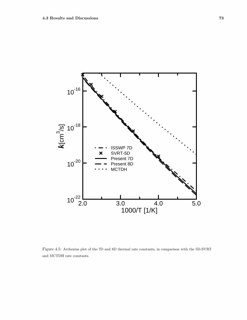
4.3 Results and Discussions 73
2.0 3.0 4.0 5.01000/T [1/K]
10-22
10-20
10-18
10-16
k[cm
3 /s]
ISSWP 7DSVRT-5DPresent 7DPresent 8DMCTDH
Figure 4.5: Arrhenius plot of the 7D and 8D thermal rate constants, in comparison with the 5D-SVRT
and MCTDH rate constants.

4.3 Results and Discussions 74
used in this calculation. It should be noted that all three moments of inertia at the transition
state geometry are quite large. The reactant partition function, which is required in Eq.(4.1), is
described as
Qr(T ) = Qrot,CH4(T )Qvib,CH4(T )Qtrans,H+CH4(T ). (4.32)
Here Qtrans,H+CH4(T ) is the partition function of the relative translational motion of the two
reactants. Qrot,CH4(T ) is the rotational partition function of methane and Qvib,CH4(T ) the vibra-
tional partition function. Within the temperature range considered, rotational and vibrational
motions of methane can be considered separable and the classical expression for the rotational
partition function can be employed. The harmonic approximation for vibrational partition func-
tion is used based on the solving of bound states for CH4. Because only the even CH bending
states occur for a non-rotating CH4 molecule, the excitation energies calculated in this study are
2880 cm−1, 2734 cm−1, 1299 cm−1, and 2947 cm−1, respectively, for the (1000), (0200), (0010),
and (0001) states. Here (vs, vb, vu, vss) denotes the CH4 state, where vs, vb, vu, and vss rep-
resent, respectively, the stretching excitation of the reactive CH bond, the bending excitation of
the reactive CH bond, the umbrella excitation of the CH3 group, and the symmetry stretching
excitation of the CH3 group. Hence the frequency used for the CH bending motion approximate
1367cm−1. In addition, in the computation of k(T ) the N(E) with energies up to 1.2eV for 7D
model and 1.4eV for 8D model is considered and also is enough to give converged k(T ) within the
temperature range of 200-500K. The corresponding Arrhenius plot for k(T ) is shown in Fig.4.5
together with previous theoretical and experimental results.
First the rate constants for these 7D and 8D models differ only by 10%-20%, which suggests
that the additional mode, i.e., the symmetry stretching motion for the CH3 group, does not
change the dynamics of the process within the temperature range of 200-500K. By comparing the
rate constants with a previous result calculated by the same 7D model but with the initial state
selected time-dependent wave packet method(ISSWP)[110], one can see a quite good agreement,
showing only 20-30% difference. One should note that the 7D ISSWP rate constant was for the
ground rovibrational initial state of CH4. Based on the fact that the vibrational excitation has
little effect on the JG PES and the assumption that initial rotational excitations of CH4 also
have little effect on the dynamics, one can approximately treat it as the thermal rate constant.
On the other hand, the present study takes into account the effect of CH4 initial rovibrational
excitations, but uses the J-K shifting approximation to yield the thermal rate constant. With
the very different approximations employed in these two calculations, the agreement between the
present and the ISSWP studies on the rate constant can be considered to be quite good. This

4.3 Results and Discussions 75
also indicates that the initial rotational excitation of CH4 does not have any important effect on
the reaction dynamics for this reaction on the JG PES. Finally, one can also see that the present
TSWP rate constant agrees with the SVRT-5D result quite well.
Now we compare these 7D and 8D rate constants with some earlier results obtained using
other approximate methods. The agreement between the present 7D/8D rates and the SVRT-5D
result is good. In the temperature region considered here, they differ by 30%. In the SVRT
approach to atom-polyatomic reactions, the reacting polyatomic molecule is treated as semi-rigid
vibrating rotors whose spatial motion is described exactly. As a result of accurate treatment
of the spatial motion, the SVRT model is capable of providing rather accurate results if the
geometry of the polyatomic molecule can be properly chosen.
However, the present 7D and 8D rate constants are much smaller by one to two orders of
magnitude than those obtained by using the MCTDH method. Since both these two results are
obtained with the J −K shifting approximation based on a total cumulative reaction probability
for J=0, the huge difference shows its special importance. As the 8D model we used in this study is
the most realistic so far for this six-atom reaction with only keeping the CH3 a C3V symmetry, the
results would be reliable if this assumption is kept very well in the low temperature range. Hence
one possible reason is that the rest four dimensions not considered in these 8D calculations, i.e.,
the two asymmetry stretching motions and two asymmetry bending motions for CH3 group, may
play some role to the rate constants. However, according to previous MCTDH calculations[111],
the difference between 8D and 12D MCTDH rate constants is less than 70% at low temperature
of 200K and even less to 35% at high temperature of 500K. So we cannot attribute the difference
between TSWP and MCTDH results only to the dimensionality. Another possible reason may
be the nature of methodologies. TSWP or ISSWP, employing Jacobi coordinates for the reaction
system, is a kind of global dynamical method, while MCTDH using normal modes explores the
potential energy surface near the vicinity of the reaction path, but ignores the global topological
details of a PES.
In addition, the accuracy of JG-PES is important for comparison between calculation and
experimental results. Recently, Manthe and coworkers have systematically constructed a PES
based on ab initio calculation at level of CCSD(T)/cc-pVTZ and employed the MCTDH method
to calculate the rates, which did give a good result only smaller by a factor of 2-4 comparing with
the experimental results but smaller by a factor of two orders of magnitude comparing with the
MCTDH results on JG-PES. This huge improvement may be the result of the increased barrier
height, because the vibrationally adiabatic barrier heights is 13.4kcal/mol for this ab initio PES

4.4 Conclusions 76
but 10.9kcal/mol for the Jordan-Gilbert PES[112]. It also presents an urgent need to calculate
the rate constants with TSWP and ISSWP approach on an accurate ab initio PES. Recently, a
new 8D PES was constructed employing the Grow package[28] based on the ab initio calculations
at level of CCSD(T) and the time-dependent wave packet calculations using both the TSWP and
ISSWP approaches will be reported on this new 8D PES soon.
4.4 Conclusions
A seven- and eight- dimensional transition state wave packet dynamics calculations have been
done to study the H+CH4 → H2+CH3 reaction on the JG-PES. We employed the reduced-
dimensional model for the X+YCZ3 type of reaction, originally proposed by Palma and Clary[13],
by restricting the CH3 group under C3V symmetry. In the seven dimensional calculations, the CH
bond length in the CH3 group is fixed at its equilibrium value of 2.067a.u. The remaining seven
degrees of freedom were included in this study exactly. In the eight dimensional calculations, all
the eight modes were included exactly. For both of these two models, we calculated the cumulative
reaction probability at J=0 for the ground state and some vibrationally excited transition states
on the dividing surface across the saddle point. Based on the obtained cumulative reaction
probabilities for J=0, the rate constants were calculated for temperature values between 200
and 500 K employing the J-shifting approximation. The 7D and 8D results agree perfectly with
each other, suggesting the additional mode for the symmetry stretching in CH3 group does not
change in reaction within the temperature range considered here. The results also show quite
good agreement with the previous 7D ISSWP rates, the 5D-SVRT rates, and experimental data,
but much smaller than the full-dimensional MCTDH results.

Chapter 5Continuous Configuration Time
Dependent Self-Consistent Field
Method(CC-TDSCF)
5.1 Introduction
In the last two chapters, we have applied time dependent transition state wavepacket approach
(TSWP) to study the four-atomic system (H2CO) and the reduced seven and eight dimensional
system of H+CH4. It is obvious that during the last two decades with development of various
efficient representation schemes[117, 37, 118] and time propagators[30, 32], the time dependent
wave packet method has became a dominant computational tool for studying complex chemical
dynamics problems with more than three degrees of freedom. It has enjoyed considerable suc-
cesses on accurate quantum reactive scattering studies of four-atom chemical reactions in full six
dimensions[25, 119, 77, 120].
The main advantage of the TD method over the traditional time-independent method is that
it scales almost linearly with the number of basis functions. However, due to the quantum nature
that number of basis functions grows exponentially with dimensionality, it is only practical at
present to deal with seven to eight strongly coupled degrees of freedom[110]. Hence, to study
quantum dynamical problems involving many atoms, one has to resort to the reduced dimension-
ality approach to cut down the number of degrees of freedom included in dynamical studies, or
77

5.1 Introduction 78
some computational approximate methods to overcome the scaling of effort with dimensionality.
A promising approach is the time-dependent self-consistent field (TDSCF) method[121, 122,
123, 124, 125, 126, 127, 128, 129, 130]. In the simplest version, i.e. the single configuration
time-dependent self-consistent field (SC-TDSCF) approach, the wavefunction of the system is
written as a direct product of the wavefunctions for subsystems[121, 122, 123, 124, 126]. A
principal drawback of SC-TDSCF is that it replaces exact interaction between subsystems by
mean-field coupling, resulting in the lack of correlations between subsystems. One way to account
for the important correlations neglected in SC-TDSCF is to add wavefunctions with different
configurations to give more flexibility to the wavefunction of the system, resulting in the so-
called multiconfiguration time-dependent self-consistent field (MC-TDSCF) method[127, 128,
129, 130, 131]. Wavefunctions with different configurations are usually constructed by imposing
orthogonal condition explicitly, making it hard to use more than a few configurations in numerical
implementation. Furthermore, the resulting equations for MC-TDSCF are very complicated
compared to those in SC-TDSCF method. For these reasons, MC-TDSCF has only been applied
to some model problems.
The closely related multiconfiguration time-dependent Hartree method (MCTDH) generalizes
MC-TDSCF in a systematic way, thus eliminating the need for choices of the TDSCF states[14,
103]. It has successfully been applied to study various realistic and complex quantum dynamical
problems (see Ref. [103] for references). Very recently, it was successfully applied to calculate the
J = 0 cumulative reaction probability for the six atom H + CH4 reaction in full 12 dimensions
on an ab initio potential energy surface (PES), from which the thermal rate constants in a
broad temperature region were obtained for the reaction[15]. However, the general application of
MCTDH method to strongly correlated systems yields a numerical method wherein the number
of possible TDSCF configuration grows exponentially with the number of degrees of freedom,
again confining practical use of the method to relatively small systems.
Recently, we proposed a new and efficient scheme for MC-TDSCF, namely, continuous-
configuration time-dependent self-consistent field (CC-TDSCF) method[104]. Very often dynami-
cal processes in polyatomic systems can be described as a system of a few strongly coupled degrees
of freedom which characterize the process of interest, coupled with clusters of bath modes. Bath
modes inside a cluster may be coupled to each other, but the coupling between bath modes in
different clusters may be neglected. The basic idea for our new method is to use discrete variable
representation (DVR)[37] for the system and then to each DVR point of the system we associate
a configuration of wavefunction in terms of direct product wavefunctions for different clusters of

5.1 Introduction 79
the bath modes. In this way, the correlations between the system and bath modes, as well as
the correlations between bath modes in each individual cluster can be described properly, while
the correlations between bath modes in different clusters are neglected. Since DVR used for the
system are orthogonal, the resulting equations are as simple in structure as those for SC-TDSCF.
The dimensionalities of the equations are determined by the number of degrees of freedom in the
system and in each individual cluster of bath modes. The method was tested on a model problem
of a one-dimensional double well linearly coupled to a harmonic bath[132, 133, 17]. It was found
to this model harmonic bath system the CC-TDSCF approach is much more accurate than the
traditional SC-TDSCF method, because it allows the bath wave function to change continuously
along the system coordinate, in contrast to the SC-TDSCF method which just uses one bath
wave function. Our test demonstrated that the CC-TDSCF approach was capable of producing
semi-quantitative, or even quantitative results.
In the present work we test CC-TDSCF method on three important complex systems: the H
+ CH4 → H2 + CH3 reaction, the hydrogen diffusion on Cu(100) surface, and the double well
coupled to a dissipative bath. The H + CH4 → H2 + CH3 reaction, due to its important roles in
CH4/O2 combustion chemistry, has been the subject of both experimental and theoretical interest
for many years. Because five of the six atoms involved are hydrogens, it is an ideal candidate for
high quality ab initio quantum chemistry calculations of the potential energy surface and quantum
dynamics studies. This reaction has become a benchmark for developing and testing various
theoretical methods to accurately study polyatomic chemical reactions[90, 91, 99, 100, 101, 109,
108, 110]. Very recently, Manthe and coworkers constructed a high quality PES for the reaction
in the vicinity of the saddle point. The PES can be used to calculate thermal rate constant
for the reaction by using flux-flux autocorrelation based methods[15]. The cumulative reaction
probabilities for the total angular momentum J=0 were calculated on the PES from which the
thermal rate constants for the reaction in a broad range of temperature were obtained. It was
found that the theoretical thermal rate constants has an accuracy comparable to or even exceeding
experimental precision. In this work we use the PES developed by Manthe and coworkers to test
the accuracy of the CC-TDSCF method for the H + CH4 reaction.
Hydrogen diffusion on metals is a phenomenon of great fundamental and technological im-
portance. Due to the small adsorbate mass, quantum-mechanical tunneling through the classical
migration barriers becomes the dominating diffusion mechanism at sufficiently low temperatures.
Recently Lauhon and Ho have studied the self diffusion of hydrogen atoms on the Cu(100) surface.
Their results reveal a sharp transition from thermally activated diffusion to quantum tunneling

5.1 Introduction 80
at T=60 K[134]. Various versions of TST approaches, as well as the quantum version of the
transition state theory developed by Miller and co-workers[135, 7], have been also developed to
study the hydrogen diffusion[136, 137, 138, 139, 16, 140]. However in most studies, the rigid sur-
face model was used, or some ab initio calculations were done to provide an optimized potential
energy for H on a flexible surface[141], that is, surface modes were neglected in their quantum
calculations. Some time ago, Zhang and Light[16] have investigated the role of surface modes in
the quantum dynamics of hydrogen diffusion at temperatures in the 120-600K range based on
a potential developed by Wonchoba and Truhlar[142] and with the transition state wave packet
approach using the flux-flux correlation function formalism for the rate constant. It was found
that eight degrees of freedom of the surrounding surface Cu atoms are needed to sufficiently damp
the recrossing of the transition state surface in order to converge the correlation expression and
determine the rate constant. In this work, we use the same system model and potential energy
surface to test the application of the CC-TDSCF method to this high-dimensional system.
The model system of a double well coupled to a dissipative bath is extensively used to study
the kinetics of a particle in common condensed phase environments. Generally the conventional
description of a reactive event in the condensed phase involves a reaction coordinate, the ’system’.
coupled to a large number of harmonic ’bath’ degrees of freedom which mimic the effects of the
environment. The most important character of this system is the Kramers turnover, i.e., the
reaction rate depends nonmonotonically on the friction, increasing at small friction (energy-
diffusion-limited regime) and eventually falling off with the friction constant when the latter
becomes large enough to ensure Boltzmann equilibrium (spatial diffusion regime). This system
has been widely studied with classical mechanical methods, quantum transition state theory, and
recently it has been used to test new quantum dynamics methodologies, in particular for those
semiclassical theory based methodologies. In this work, we apply the CC-TDSCF and exact
TSWP approaches to study the reaction rate for the barrier crossing of a proton based on the
flux-flux correlation function calculations.
In the following section we introduce the CC-TDSCF method in a general form. In Sec.
III, we then present the results for H+CH4 with some seven dimensional calculations and ten
dimensional calculations by using the approximation CC-TDSCF method, in comparison with
the results from exact calculations. In Sec. IV, we report the results for the hydrogen diffusion
on Cu(100) surface with CC-TDSCF method. In Sec. V, the results for the double well coupled
to a dissipative bath are presented.

5.2 Theory 81
5.2 Theory
5.2.1 CC-TDSCF Method
Consider a general multidimensional problem with Hamiltonian written as
H(s,x1,x2, ...,xN ) = h(s) +N∑
i
h(xi) + V(s,x1,x2, ...,xN ), (5.1)
where s and xi (i = 1, ..., N) are multidimensional vectors, with dimension equal to ns and ni,
respectively. We call s as system coordinates, and xi as ith cluster of bath coordinates. Hence
the total dimension of the problem is ns +∑N
i ni. We partition it into an ns dimensional system
and N clusters of bath modes. In Eq. 5.1, the Hamiltonians for system s and bath cluster xi are
given by
h(s) =
ns∑
j
[
T (sj) + V (sj)]
=
ns∑
j
h(sj), (5.2)
h(xi) =
nj∑
j
[
T (xij) + V (xi
j)]
=
nj∑
j
h(xij), (5.3)
where T is the kinetic energy operator, V (x) is the one dimensional reference for coordinate x.
The CC-TDSCF ansatz for the total wave function is written as follows[104]
Ψ(s,x1, · · · ,xN , t) =
M∑
α=1
Cα(t) |sα〉Φα(x1, · · · ,xN , t), (5.4)
where |sα〉 denotes DVR points for the system coordinates s which is constructed via direct prod-
uct of DVR grids for individual coordinate si (i = 1, ..., ns); Φα(x1, · · · ,xN , t), which depends on
the DVR point |sα〉, is written as a product of single-mode functions as in the single configuration
TDSCF,
Φα(x1, · · · ,xN , t) =
N∏
i=1
φiα(xi, t), (5.5)
where φiα(xi, t) is the time-dependent wave function for the ith cluster of bath coordinates, xi,
at |sα〉 DVR point for the system coordinates. It has the following the constraints
〈φiα(t)| ∂
∂tφi
α(t)〉 = 0, and 〈φiα(0)|φi
α(0)〉 = 1, (5.6)
for i = 1, 2, · · · , N . These constraints will guarantee that the single-mode functions are normalized
at any time t.

5.2 Theory 82
Now we introduce the “single-hole function”:
Φ(i)α = φ1
α · · ·φ(i−1)α φ(i+1)
α · · ·φNα , (5.7)
then Φα in Eq. 5.5 can be written as
Φα = φiα Φ(i)
α . (5.8)
Employing the Dirac-Frenkel variational principle[143], we can get the equations of motions
as[104]
i Cα =∑
β
〈sαΦα|H |sβΦβ〉Cβ , for α = 1, · · · ,M ; (5.9)
i[
Cα φiα + Cα φ
iα
]
=∑
β
〈sαΦ(i)α |H |sβΦ
(i)β 〉[
Cβ φiβ
]
, (5.10)
for i = 1, 2, · · · , N.
By defining a new function,
ϕiα = Cα φ
iα, (5.11)
we can rewrite Eq. 5.10 as
iϕiα =
∑
β
〈sαΦ(i)α |H |sβΦ
(i)β 〉ϕi
β , i = 1, · · · , N. (5.12)
The single-mode function φiα can be obtained by multiplying C∗
α on both sides of Eq. 5.11 and
resorting the normalization conditions for the single-mode functions,
C∗αϕ
iα = |Cα|2 φi
α, =⇒ φiα =
C∗αϕ
iα
||C∗αϕ
iα||, (5.13)
where ||f || =√
〈f |f〉 denotes the modulo of a function.
We can see from Eq.5.9 that the evolution of Ci in Eq.5.9 is governed by an effective Hamil-
tonian arising from averaging the total Hamiltonian over all the bath modes at each DVR point
in the system coordinates, while the evolution of wave function for the ith cluster of bath modes
is governed by an effective Hamiltonian arising from averaging the total Hamiltonian over all the
bath clusters except itself (ith mode) on each DVR point in the system coordinates. Hence to
propagate the total wave function, one needs to solve an ns dimensional equation for the system,
and N equations for all the N bath clusters with a dimension equal to ns +ni for the ith cluster.

5.2 Theory 83
5.2.2 Propagation of CC-TDSCF equations
To propagate CC-TDSCF equations given in Eq. 5.9 and 5.12, one need to calculate the av-
erages of Hamiltonian over wavefunctions. Let us first take a look at the average in Eq. 5.12.
Substituting the Hamiltonian given in Eq. 5.1 into the average, we can get
〈sαΦ(i)α |H |sβΦ
(i)β 〉 = 〈sαΦ(i)
α
∣
∣
∣
∣
∣
h(s) +
N∑
k
h(xk) + V(s,x1,x2, ...,xN )
∣
∣
∣
∣
∣
sβΦ(i)β 〉
= 〈sα|h(s)|sβ〉〈Φ(i)α |Φ(i)
β 〉 +
[
N∑
k
〈Φ(i)α |h(xk)|Φ(i)
α 〉 + 〈Φ(i)α |V(sα,x
1,x2, ...,xN )|Φ(i)α 〉]
δα,β
= 〈sα|h(s)|sβ〉〈Φ(i)α |Φ(i)
β 〉 +
h(xi) +N∑
k 6=i
Eeffα (xk) + V eff (sα,x
i)
δα,β, (5.14)
where
Eeffα (xk) = 〈φk
α(xk, t)|h(xk)|φkα(xk, t)〉, (5.15)
with φkα(xk, t) given in Eq. 5.5, is the expectation value of Hamiltonian, or, energy for ith bath
cluster at |sα〉 DVR point. Veff (sα,xi) in Eq. 5.14 is the effective potential at system DVR |sα〉
and coordinates for ith bath cluster xi.
To discuss the first term in Eq. 5.14, we write a system DVR point |α〉 as |skµ〉|α(k)〉, with
|skµ〉 denoting the µth DVR point for kth system coordinate, |α(k)〉 denoting the corresponding
DVR points for the other coordinates in the system. For kth system coordinate, we have,
〈skµ|〈α(k)|h(sk)|skν〉|β(k)〉〈Φ(i)
skµα(k) |Φ(i)
skνβ(k)〉 = 〈skµ|h(sk)|skν〉〈Φ(i)
skµα(k) |Φ(i)
skν β(k)〉δα(k)β(k) . (5.16)
Hence 〈sα|h(s)|sβ〉〈Φ(i)α |Φ(i)
β 〉 matrix is block diagonal for each system coordinate as in ordinary
DVR representation. But the matrix for each system coordinate is now time-dependent, in
contrast to that in ordinary DVR representation.
Once having matrix elements for 〈sαΦ(i)α |H |sβΦ
(i)β 〉, it is straightforward to do one more
integration with the wave function for ith bath cluster to get
〈sαΦα|H |sβΦβ〉 = 〈φiα|〈sαΦ(i)
α |H |sβΦ(i)β 〉|φi
β〉
= 〈sα|h(s)|sβ〉〈Φα|Φβ〉 +
[
N∑
k
Eeffα (xk) + V eff (sα)
]
δα,β. (5.17)
With matrix elements for 〈sαΦα|H |sβΦβ〉 and 〈sαΦ(i)α |H |sβΦ
(i)β 〉 written down, we can prop-
agate the equations of motion for Cα(t) and φiα. We use split-operator method to carry out
these propagations. Everything is very straightforward, as in ordinary DVR based wave packet

5.3 Application to the H + CH4 System 84
propagation, except that the Hamiltonians involved now are time-dependent. So we have to diag-
onalize relevant matrices at every step. This may produce a bottleneck for computational speed
if the maximum number of DVR points used for one system coordinate becomes large. While
in the current applications this number is around 50, so it does not cause any problem to the
computation.
5.3 Application to the H + CH4 System
5.3.1 Theory
The thermal rate constant, k(T ), can be calculated from the time integral of a flux-flux autocor-
relation function[16, 144, 145]
k(T ) = Qr(T )−1
∫ ∞
−∞
dtCff (t), (5.18)
where Qr(T ) is the reactant partition function,
Cff (t) = tr[F eiHt∗c F e−iHtc ] =∑
n=0
Cnff (t), (5.19)
and tc = t − iβ/2 with β = (kBT )−1. Cnff is defined as the autocorrelation function for the
nth transition state wave packet[16]. In present study, we focus on the flux-flux autocorrelation
function for its ground transition state wave packet[16],
Cff (t) = C0ff (t) = 〈ψg(t)|F |ψg(t)〉. (5.20)
The wave function ψg(t) for the ground state transition state wave packet is given by,
ψg(t) = e−iHte−Hβ/2√λ|+〉|g0(s′)g1(x1) · · · gN (xN )〉, (5.21)
where |gk(xk)〉(k = 1, 2, ..., N) is the ground state wave function for hk(xk), |+〉 is the flux
operator eigenfunction with non-zero eigenvalue of λ for coordinate perpendicular to the dividing
surface in system, |g0(s′)〉 is the ground state wave function on the dividing surface s′. From Eq.
5.21, one can see that we first propagate each transition state wave packet in imaginary time to
β/2, and then propagate it in real time.
Following Manthe and coworkers[90, 91, 15], we use transition state normal coordinate system
in our calculation to minimize correlation effects in the transition state region. Normal modes
and normal coordinates were calculated at the transition state geometry and the corresponding

5.3 Application to the H + CH4 System 85
linear transformation matrix was used throughout the calculation to convert the working coor-
dinates into Cartesian coordinates. The transition state for the reaction, Ha-Hb-CH3, is of C3v
symmetry with Ha-Hb-C lying on the C3v symmetry axis. Here we labelled two hydrogen atoms
involving in reaction to distinguish them from three other hydrogen atoms in the CH3 group.
For such a system of six atoms, there are 12 normal vibrational modes. They are the imaginary
mode (Q1) concerning the asymmetric stretching motion of the Ha-Hb-CH3 fragments on the C3v
symmetry axis, a doubly degenerate low-frequency bending modes (Q2,Q3) mainly involving the
motion of Ha atom, an umbrella mode (Q4) for the non-reacting CH3 group, a doubly degenerate
high-frequency bending modes (Q5,Q6) mainly involving the motion of Hb atom, another doubly
degenerate bending modes (Q7,Q8) essentially involving the motion of the hydrogens in nonre-
acting CH3 group, a symmetric stretching mode (Q9) of the Ha-Hb-CH3 fragments on the C3v
symmetry axis, and a symmetric (Q10) and doubly degenerate asymmetric stretches (Q11,Q12)
concerning mainly the nonreacting CH3 group. Among all these modes, Q1 and Q9 are directly
relevant to the reaction.
With mixed derivatives in the kinetic energy resulting from vibrational angular momentum
neglected, the Hamiltonian for the system can be simply written as
H(Q1, Q2, · · · , Q12) =
12∑
i=1
−1
2
∂2
∂Q2i
+ V(Q1, Q2, · · · , Q12)
=
12∑
i=1
hi(Qi) + V (Q1, Q2, · · · , Q12), (5.22)
where
hi(Qi) = −1
2
∂2
∂Q2i
+ Vi(Qi) (5.23)
is the one-dimensional Hamiltonian for these normal modes. The reference potential Vi(Qi) for
mode i is taken as
Vi(Qi) = 0, for Q1, Q4, and Q9
Vi(Qi) = V(Q1 = 0, · · · , Qi, · · · , Q12 = 0) for other coordinates.
To choose a proper dividing surface, we define two new coordinates Q′1 and Q′
9 by rotating
Q1 and Q9 coordinates by an angle θ = 25◦,
Q′1 = sin θ Q1 + cos θ Q9
Q′9 = cos θ Q1 − sin θ Q9.
The dividing surface is located as Q′1 = 0 in our calculation.

5.3 Application to the H + CH4 System 86
-100 -50 0 50 100-50
0
50
100
150
x
2 1.5 1
0.8 0.7 0.64 0.6 0.5 0.4 0.3 0.2 0.1
Q1’
Q9’
Figure 5.1: The minimum potential energy surface projected on the normal coordinates for Q′
1 and Q′
9
with energy minimized on the other coordinates. The unit for the coordinates is bohr· amu1/2 and for
energy is eV.
5.3.2 Numerical Details
To check the accuracy of the CC-TDSCF method, we need to calculate the autocorrelation
functions by using exact quantum dynamics method. With the computer available to us, we are
able to include up to ten of out the total twelve degrees of freedom. Intensive tests reveal that the
doubly degenerate bending modes (Q7,Q8) involving the motion of the hydrogens in nonreacting
CH3 group essentially play no role in the dynamics, hence are excluded in this study. We use 49
sine-DVR in a range of [-120,120] for Q1, 13 sine-DVR in a range of [-100,50] for Q4, 29 sine-DVR
in a range of [-50,150] for Q9. For Q2, Q3, Q5, Q6, Q11, and Q12, we use 5 potential optimized
DVR (PODVR)[38], and for Q10, we use 6 PODVR. Hence the basis number used in the exact
ten-dimensional quantum dynamics calculation reaches 1.7 × 10⁹. The temperature considered
in this study is 500 K. We propagate wave packet 50 steps for imaginary time propagation in Eq.
5.21. For real time propagation, the time step is 5 a.u. for the exact calculation, 1 a.u. for the
CC-TDSCF method because of the self-consistent nature of the method.

5.3 Application to the H + CH4 System 87
5.3.3 Seven-dimensional (7D) Results
We first test the CC-TDSCF method on seven low frequency modes, i.e. Q1, Q2, Q3, Q4, Q5, Q6,
and Q9. In the CC-TDSCF calculation, we choose Q1 and Q9 as the system coordinates s. The
other five coordinates involved, Q2, Q3, Q4, Q5, Q6, are treated as five bath clusters, i.e. with
one coordinate in every bath cluster. In the work, we use {(1, 9), (2), (3), (4), (5), (6)} to denote
this kind of partition in coordinates, with the numbers in the first pair of parentheses referring
the system coordinates, and the number(s) in the following pairs of parentheses referring the
coordinate(s) in each bath cluster. Under this partition, one needs to solve one two-dimensional
equation for the system, plus five three-dimensional equations for the bath clusters.
0.0 500.0 1000.0Time (a.u.)
0.0
0.5
1.0
1.5
Cff (
x10
−14 )
exact 7D{(1,9)(4)(5)(6)(2)(3)}
Figure 5.2: Cff as a function of real time propagation for the ground transition state by using both exact
quantum method and CC-TDSCF method with Q1, Q2, Q3, Q4, Q5, Q6, Q9 included in calculations.
Fig.5.2 shows Cff as a function of real time propagation, t, for the ground transition state
by using both exact quantum method and CC-TDSCF method. The exact Cff shown in Fig.5.2
exhibits a typical behavior for the flux-flux autocorrelation function for a direct reaction: it decays
quickly as time increases, goes through zero at t ∼ 300 a.u., then becomes a little bit negative,
and finally gets stabilized at zero at t ∼ 700 a.u. Hence for the temperature considered here,
recrossing in flux-flux autocorrelation does occur, although it is not substantial. From Fig.5.2,

5.3 Application to the H + CH4 System 88
we can see that overall agreement between the CC-TDSCF Cff and the exact one is quite good.
At t = 0, it is about 12% smaller than the exact Cff . It decays slightly slower than the exact
Cff , hence crosses with the exact Cff curve at t ∼ 220 a.u. The CC-TDSCF Cff also moves in
and out of the recrossing region slightly slower than the exact one.
It is quite interesting to see that the largest difference between CC-TDSCF and exact Cff
is at t = 0, right after the imaginary time propagation. Neglecting of correlations between bath
modes prevent the whole system from relaxing as in the exact treatment during imaginary time
propagation, making the CC-TDSCF Cff at t = 0 smaller than the exact one. While during the
real time propagation, neglecting of correlations between bath modes makes the whole system
slower in dissipating energy and in moving away from the dividing surface. As a result, the
CC-TDSCF Cff decays slightly slower than the exact one as shown in Fig.5.2.
0.0 500.0 1000.0Time (a.u.)
0.0
1.0
2.0
Cfs
(x10
−12 )
exact 7D{(1,9)(4)(5)(6)(2)(3)}{(1,9)(4)(2,5)(3,6)}{(1,9,4)(2,5)(3,6)}
Figure 5.3: Cfs as a function of real time propagation for the ground transition state by using both exact
quantum method and CC-TDSCF method with Q1, Q2, Q3, Q4, Q5, Q6, Q9 included in calculations.
Fig.5.3 shows the exact and CC-TDSCF Cfs as a function of time by integrating the Cff
function shown in Fig.5.2. The curves look very similar, except that the CC-TDSCF Cfs is lower
than the exact one. At t ∼ 300 a.u. when they reach their maximum values, the CC-TDSCF Cfs
is about 9% smaller than the exact one. The difference increases to 12% at t ∼ 700 a.u. when
they are stabilized. Thus the CC-TDSCF method introduces an error of 12% by approximating

5.3 Application to the H + CH4 System 89
a seven-dimensional problem with one two-dimensional plus five three-dimensional problems.
Under the {(1, 9), (2), (3), (4), (5), (6)} partition, we only took into account the correlations
between system coordinates and individual bath coordinate, while neglected the correlations
between bath coordinates. To investigate the importance of the correlations between bath co-
ordinates, we carried many calculations by using different partition of the coordinates. It was
found that the Ha bending modes Q2 and Q3 have substantial correlations with the Hb bending
modes Q5 and Q6 on the same plane, i.e. Q2 correlates Q5, Q3 correlates with Q6. Thus an
higher accuracy may be achieved by putting Q2 and Q5 in one bath cluster, Q3 and Q6 in another
bath cluster. As we can see from Fig.5.3 that CC-TDSCF Cfs with the {(1, 9), (4), (2, 5), (3, 6)}partition is considerably more accurate than that with the {(1, 9), (2), (3), (4), (5), (6)} partition,
when compared to the exact result. It is only smaller than the exact result by 3.5%. Under this
partition, one needs to solve one two-dimensional equation for the system, one three-dimensional
equation for Q4, two four-dimensional equations for (Q2, Q5) and (Q3, Q6). If we put the um-
brella mode Q4 in the system, i.e. with a {(1, 9, 4), (2, 5), (3, 6)} partition, we can further reduce
the difference between the CC-TDSCF and exact Cfs to 2%. As we can see from Fig.5.3 that
the CC-TDSCF Cfs with the {(1, 9, 4), (2, 5), (3, 6)} partition is essentially identical to the exact
one, indicating that there is very little correlation between (Q2, Q5) and (Q3, Q6) clusters. An-
other way to improve the accuracy of the {(1, 9), (4), (2, 5), (3, 6)} partition is to move Q2 and Q3
modes to the system, resulting a {(1, 9, 2, 3), (4), (5), (6)} partition. Fig.5.3 shows that the ac-
curacy of the {(1, 9, 2, 3), (4), (5), (6)} partition is very close to that of the {(1, 9, 4), (2, 5), (3, 6)}partition. Compared to the {(1, 9), (4), (2, 5), (3, 6)} partition, the {(1, 9, 4), (2, 5), (3, 6)} parti-
tion takes into account the correlations between Q4 mode and Q2, Q3, Q5, Q6 modes, while
the {(1, 9, 2, 3), (4), (5), (6)} partition takes into account the correlation between Q4 mode and
Q2, Q3 modes, the correlations between Q2 and Q6, Q3 and Q5. The close agreement between
the {(1, 9, 4), (2, 5), (3, 6)} partition and the {(1, 9, 2, 3), (4), (5), (6)} partition indicates to some
extend that the correlation between Q4 mode and Q2, Q3 modes are more important than the
correlation between Q4 mode and Q5, Q6 modes.
5.3.4 Ten Dimensional (10D) Results
Fig.5.4 and Fig.5.5 shows Cff and Cfs, respectively, as a function of real time propagation, t, for
the ground transition state by using both exact quantum method and CC-TDSCF method with
Q10, Q11, and Q12 included in dynamical calculations. Before comparing the exact 10D result
with the CC-TDSCF ones, let us make a comparison between the 7D and 10D exact results shown

5.3 Application to the H + CH4 System 90
0.0 500.0 1000.0Time (a.u.)
0.0
1.0
2.0
3.0
Cff
(x10
−14 )
exact 10D{(1,9)(4)(5)(6)(2)(3)(10)(11)(12)}
Figure 5.4: Same as Fig.5.2 except with three high frequency modes, Q10, Q11, and Q12 included.
in Fig.5.2 and 5.4. In our calculations, we set the ground state energy for every degree of freedom
included in the calculation to be zero. Hence, if a degree of freedom plays no role to the dynamics,
Cff will only change very little (due to potential average effect) when that degree of freedom is
included in dynamics calculations. Fig.5.4 show that the exact Cff changes substantially when
Q10, Q11, and Q12 are included in dynamical calculation. At t = 0, the 10D Cff in Fig.5.4 is
larger than 7D Cff in Fig. 5.2 by about 60%. For the corresponding Cfs shown in Fig.5.3 and
Fig.5.5, the 10D Cfs is about 50% larger than the 7D Cfs. It is well known that there is some
kind of mixing between these stretching modes and the umbrella mode in normal coordinates, in
particular at geometries far way from the reference geometry. Hence freezing stretch modes as
in the 7D calculation may substantially underestimate Cfs, as discussed by Miller and coworkers
in the H2 + OH system[146].
As in the 7D case shown in Fig.5.2, we carried out a CC-TDSCF calculation with a {(1, 9), (2),
(3), (4), (5), (6), (10), (11), (12)} partition. The comparison between the exact 10D Cff and the
CC-TDSCF one shown in Fig.5.4 is very similar to that in Fig.5.2, except that the difference
between these two curves increases. At t = 0, the exact one is larger than the CC-TDSCF one by
22%. Consequently, the difference in Cfs between them shown in Fig.5.5 also increases compared

5.3 Application to the H + CH4 System 91
0.0 500.0 1000.0Time (a.u.)
0.0
1.0
2.0
3.0
4.0
Cfs (
x10
−12 )
exact 10D{(1,9)(4)(5)(6)(2)(3)(10)(11)(12)}{(1,9)(4)(2,5)(3,6)(10,11,12)}{(1,9,2,3)(4)(5)(6)(10,11,12)}
Figure 5.5: Same as Fig.5.3 except with three high frequency modes, Q10, Q11, and Q12 included.
to that in 7D. When stabilized, the exact Cfs is about 22% larger than the CC-TDSCF one.
Thus, these three high frequency modes also have some strong correlations with themselves or
other modes. Once again, we can see that the CC-TDSCF Cff decays slower than the exact one
as in 7D case, and it becomes slightly larger than the exact one at t ∼ 230 a.u. for the reason
discussed.
As in 7D calculations shown in Fig.5.3, bath modes are combined together as clusters to
take into account the correlations between them. One partition we tried is {(1, 9),(4),(2, 5),(3, 6),
(10, 11, 12)} following the 7D calculation, with additional three high frequency modes put in
one cluster. As we can see from Fig.5.5 that the {(1, 9), (4), (2, 5), (3, 6), (10, 11, 12)} partition
is considerably more accurate than the {(1, 9), (2), (3), (4), (5), (6), (10), (11), (12)}. It cuts the
error of the later partition by half to about 11%, compared to the exact result. But this error is
obviously larger than that of 3.5% for the {(1, 9), (4), (2, 5), (3, 6)} partition, indicating Q10, Q11,
and Q12 modes not only correlate among themselves, they also correlate to other modes.
After intensive tests, we found that Q10, Q11, and Q12 also correlate with Q2 and Q3 modes.
Since Q2(Q3) correlates with Q4, Q5, Q6 modes to some extend, one way to take into account all
the correlations Q2 and Q3 have with Q4, Q5, Q6, Q10, Q11, and Q12 modes is to put Q2 and Q3

5.3 Application to the H + CH4 System 92
in the system, resulting in a {(1, 9, 2, 3), (4), (5), (6), (10, 11, 12)} partition. Under this partition,
one needs to solve one four-dimensional equation for the system, three five-dimensional equation
for Q4, Q5, and Q6, and one seven-dimensional equation for Q10, Q11, and Q12. It sounds quite
expansive to solve these equations, but compared to solving the original ten-dimensional equation,
the computational effort involved here is substantially reduced because the number of basis used
in the exact 10D calculations is 13×5×5 = 325 times larger than that for the seven-dimensional
equation. For the basis set used in this study, the CC-TDSCF calculation is about a factor of
10 faster than the exact one. As we can see from Fig.5.5 that The CC-TDSCF Cfs with the
{(1, 9, 2, 3), (4), (5), (6), (10, 11, 12)} partition agrees with the exact one rather well. It is only
smaller than the exact one by 6% at t = 700 a.u.
5.3.5 Conclusions
We calculated the flux-flux autocorrelation functions for the H + CH4 reaction by using the exact
quantum dynamics method and CC-TDSCF method on the potential energy surface recently
developed by Manthe and coworkers. Since Q7 and Q8 are not important to the dynamics, we
did not include them in present study. For the remaining ten modes, we carried two sets of
calculations, one with seven low frequency modes, Q1−Q6, and Q9 included, the other including
all these ten modes.
Comparison of flux-flux autocorrelation functions obtained by using the exact dynamics
method and the CC-TDSCF method revealed that the CC-TDSCF method is capable of pro-
ducing very accurate results. For the 7D case, the largest difference between the exact one
and the CC-TDSCF one is 12% when the five bath modes were treated as five bath clus-
ters in the {(1, 9), (2), (3), (4), (5), (6)} partition. This error was reduced to 3.5% when the
{(1, 9), (4), (2, 5), (3, 6)} partition was employed. The CC-TDSCF method gave an error of 2%
with the {(1, 4, 9), (2, 5), (3, 6)} partition. When the three high frequency modes Q10, Q11, and
Q12 were included in dynamics calculations, a simple {(1, 9), (2), (3), (4), (5), (6), (10), (11), (12)}partition gave an error of 22%, indicating these three high frequency modes have some strong
correlations among themselves and/or with other bath modes. By using a {(1, 9),(4),(2, 5),(3, 6),
(10, 11, 12)} partition, we can reduce the error to 11%. The error can be reduced further to 6%
by putting Q2 and Q3 in the system in a {(1, 9, 2, 3), (4), (5), (6), (10, 11, 12)} partition.
All these calculations clearly showed that the CC-TDSCF method is a very powerful approx-
imation quantum dynamics method. It allows us to partition a big problem into several smaller
ones. By changing partition systematically, one can investigate the correlations between different

5.4 Application to the H Diffusion on Cu(100) Surface 93
degrees of freedom. By grouping modes with strong correlations together as a cluster, one can
systematically improve accuracy of the result. And by choosing the system and bath clusters
carefully, one can always keep the number of dimensions in CC-TDSCF within the computational
power resource.
5.4 Application to the H Diffusion on Cu(100) Surface
The diffusion dynamics of a H atom on the Cu(100) surface in the uncorrelated hopping regime
has already been investigated by Zhang and Light[16] using the transition state wave packet
(TSWP) approach and the flux-flux correlation function to calculate the thermal rate constant.
This time-dependent quantum simulation showed that the motions of the surface are important
to damp the recrossing of the transition state surface in order to converge the correlation function
and determine the hopping rate. However, due to the demanding nature of quantum dynamical
calculations, only up to eight degrees of freedom for the surrounding surface were included, even
though the inclusion of eight degrees of freedom are sufficient to damp the recrossing. Since
the scale of CC-TDSCF approximation approach is determined by the product of the number of
basis functions for system modes and the sum of the numbers of basis functions for each bath
cluster, this smaller number, compared to that of the exact TSWP, shows its potential to solve
this problem. We first have to check the possibility of its applications to this kind of systems. In
this work we calculated the flux-flux autocorrelation functions by using both the exact quantum
dynamics approach and CC-TDSCF approach for comparison.
5.4.1 System Model and Potential Energy Surface
Following the previous work, we use the same model system and potential energy surface to
study hydrogen diffusion on Cu(100) surface, i.e., the potential energy surface is approximated
as the sum of Morse-spline potentials for both the H-Cu and Cu-Cu pair interactions as used by
Wonchoba and Truhlar [142] (WT). The functional form is
V (R) =
D[(1 − e−α(R−Re))2 − 1], R ≤ Rc −Dc
∑i=5i=3 Ci(R−Rc −Dc)
i, Rc −Dc ≤ R ≤ Rc +Dc
0, R > Rc +Dc
(5.24)
where R is the Cu-Cu or H-Cu interatomic distance, D, α, and Re are Morse parameters, and
Rc, Dc, and Ci control the spline fits. The potential cutoff is Rc +Dc. All the parameters are
shown in Table I for easy reference.

5.4 Application to the H Diffusion on Cu(100) Surface 94
Table 5.1: Parameters used for Cu-Cu and H-Cu pair potentials
Parameter Cu-Cu H-Cu
α(◦
A−1
) 2.287 1.43
D(eV ) 0.40926 0.31602
Re(◦
A) 2.578942 2.34
Rc(◦
A) 5.157883 7.02
C3(eV◦
A−3
) 19.39 6.7049
C4(eV◦
A−4
) 270.24 94.05
C5(eV◦
A−5
) 1013.54 353.68
Dc(◦
A) 0.0529 0.0529
A lattice constant of d = 3.5818◦
A is also used by minimizing the interaction potential between
a Cu atom and all its neighboring Cu atoms within distanceRc+Dc as done by Zhang and Truhlar
[142]. This value is close to the experimental lattice constant of 3.61◦
A for Cu. Thus the nearest
neighbor distance between two Cu atoms on the (100) surface is a = d/√
(2) = 2.5327◦
A, and
the interplanar distance is d/2 = 1.7909◦
A. The Cu atoms on the surface are further relaxed
with the distance between the first and second (100) plane of Cu atoms increased by 0.0267◦
A so
that the surface Cu atoms are in their equilibrium positions in the direction perpendicular to the
surface.
In this model system, only six of the Cu atoms in the lattice are allowed to move, but the
rest of the Cu atoms are held fixed at the positions described above to provide a surrounding
framework for the mobile Cu atoms. The surrounding set of atoms extends far enough in all
directions such that it includes all bulk lattice sites within the cutoff distance of the interaction
potential to any movable Cu atom. Thus the lattice is effectively infinite, and any further increase
in the lattice of fixed Cu atoms will not have any effect on the movable Cu atoms or the H atom.
Figure 5.6 shows the geometry of the six mobile Cu atoms labelled from 1 to 6 which will be
explicitly included in the quantum calculations, together with the two equilibrium binding sites of
H denoted as R (reactant) and P (product). The surface diffusion process to be modelled consists
of the H atom hopping from site R to site P . The saddle point for this hopping process is denoted
by S in Fig.5.6. Similarly, these six mobile Cu atoms are divided into three groups, (1, 2), (3, 4),

5.4 Application to the H Diffusion on Cu(100) Surface 95
Figure 5.6: Reactant site (R), saddle point (S), product site (P), and the hopping path for diffusion of
an H adatom on the Cu(100) surface. The six nearest neighbor Cu atoms to the saddle point are labeled
from 1 to 6. The coordinate system for the H atom is also shown.
and (5, 6). For each group of Cu atoms, there are a total of six degrees of freedom. These six
individual degrees of freedom are combined into vibrational modes of relative and center of mass
motion for each pair as we do for a two particle system. For example, for the (1, 2) group the
original six degrees of freedom are denoted as (xi, yi, zi) (i = 1, 2), measured as the displacement
of a Cu atom away from its original given position. The modes of relative and center of mass
motions are then defined as,
x12 = x1 − x2; X12 =x1 + x2
2,
y12 = y1 − y2; Y 12 =y1 + y2
2,
z12 = z1 − z2; Z12 =z1 + z2
2, (5.25)
To calculate k(T ), we choose x = 0 to be the surface dividing the two unit cells surrounded by
the six movable Cu atoms as shown in Fig.5.6. On this dividing surface we construct the transition
state wave packets and measure the flux correlation functions. With this dividing surface the
system is symmetric with respect to x = 0 provided we treat the (identical) (1,2) and the (5,6)
Cu groups equally. Therefore, we can calculate the thermal rate constant by propagating the
wave packets from 0 to a time t when the time integral of the correlation function is converged.
In order to facilitate monitoring the convergence the time integral, in most cases, we will show
the integral of Ciff (T, t) with time,
Cifs(t) =
∫ t
0
Ciff (T, t′)dt′ (5.26)

5.4 Application to the H Diffusion on Cu(100) Surface 96
It is important to note that only when the system is symmetric with respect to the dividing
surface, is Cifs(∞) directly related to k(T ). Otherwise, Ci
fs(t) is just a notation for the integral
of Ciff (T, t) from time 0 to t.
5.4.2 Numerical Details
The results presented here are for T = 300K. The H atom is restricted to the two unit cells
surrounding the saddle point where the initial wave packets are constructed as shown in Fig.5.6
because we are only concerned with diffusion due to the uncorrelated hops between neighboring
unit cells. The range of the z coordinate is [1.0, 4.8]a0. The number of steps used to propagate
a transition state wave packet by β/2 varies with temperature. At T = 300K, 30 steps are used.
For the real time propagation, we use ∆t = 15a.u. for exact transition state wave packet study
and ∆ = 5a.u. for continuous configuration time-dependent self-consistent field (CC-TDSCF)
study.
5.4.3 Results and Discussions
-5 -4 -3 -2 -1 0 1 2 3 4 5-2.5
-2
-1.5
-1
-0.5
0
0.5
1
1.5
2
2.5 0.8 0.7 0.6 0.5 0.4 0.3 0.2 0.1
X (Bohr)
Y (Bohr)
Figure 5.7: The minimum potential energy surface projected on the coordinates for xH and yH with
energy minimized on the other nine coordinates (zH , X12, y12, Z12, X56, y56, Z56, X34, y34, Z34). The
unit for energy is eV.
In order to describe the diffusion of hydrogen on the mobile Cu surface, there are three degrees
of freedom to describe the motions of the H adatom at x, y, and z directions and eighteen degrees
of freedom defined in Eq.(5.25) to describe the six mobile Cu atoms, including the six modes for

5.4 Application to the H Diffusion on Cu(100) Surface 97
-5 -4 -3 -2 -1 0 1 2 3 4 5 0
0.5
1
1.5
2
2.5
3
3.5
4
4.5
5 3 2.5 2 1.5 1 0.9 0.8 0.7 0.6 0.5 0.4 0.3 0.2 0.1
X
Y
Figure 5.8: The minimum potential energy surface projected on the coordinates for xH and zH with
energy minimized on the other nine coordinates (yH , X12, y12, Z12, X56, y56, Z56, X34, y34, Z34). The
unit for energy is eV.
the (1,2) Cu group, for the (3,4) Cu group and for the (5,6) Cu group. As reported, for the (1,2)
Cu group or (5,6) Cu group, there are three of six modes which are significantly excited during
the propagation of the transition state wave packet. They are the center of mass mode in the x
direction (X12 or X56), the relative motion in the y direction (y12 or y56), and the center of mass
mode in the z direction (Z12 or Z56). The other three modes essentially remain in their ground
states. This suggests that the six surface modes for the (1,2) Cu group and (5,6) Cu group (X12,
y12, Z12, X56, y56, and Z56) are much strongly coupled the motion of the H adatom. It can be
understood easily in a classical picture with the help of Fig.5.6. When the H atom falls from the
saddle point, it will move on the y = 0 plane toward the binding site (R or P) and get close to
the (1,2) or (5,6) Cu group. The forces from the H atom on the 1 and 2 Cu pair (or 5 and 6 Cu
pair) have the same magnitude and direction on the two atoms in the x and z directions, but are
opposed in the y direction. Thus in x and z, the H atom pushes the 1 and 2 Cu atoms (or 5 and
6 Cu atoms) in the same direction, exciting the center of mass motions, but in the y direction
relative motion is excited. However, the motions for the (3,4) Cu pair are different from the (1,2)
Cu group and (5,6) Cu group, since they are the unique ”transition state pair”. The excitation
of the Cu pair in the x direction is very mild compared to that for the other two Cu groups. The
relative motion in the y direction (y34) and the center of mass mode in the z direction (Z34) are
also strongly coupled with the hydrogen motion. So there are eight surface modes (X12, y12, Z12,
X56, y56, Z56, y34, Z34) strongly coupled with the motion of the H atom and two modes (X34 and

5.4 Application to the H Diffusion on Cu(100) Surface 98
z34) are mildly coupled, while the rest surface modes are weakly coupled. In this study, we have
used two sets of modes to compare the calculation results with the exact transition state wave
packet method and the CC-TDSCF method. One set of modes includes the hydrogen motion on
x and z direction and the eight important surface modes and X34. This is reasonable because
the diffusion of the H adatom from the saddle point to reactant site or the product site is on the
xz plane and we then could consider only these two motions to save calculation time. The other
set of modes includes the hydrogen motions on x, y, z directions and the eight important surface
modes as previous work. In addition, the range of the H atom motion is limited to two unit cells,
because we also want to see only how the energy of the H atom can transfer to the Cu motion
to stabilize Cfs. For each of these Cu modes, we use three to four vibrational states which are
obtained from the optimized configuration of the system with the H adatom on the saddle point.
This guarantees that the Cu vibrations are not excited when the H atom sits on the saddle point.
0 4000 8000 12000 16000time (a.u.)
0.0
2.0
4.0
6.0
8.0
Cff
0 ( x
10-1
9 a.u
. )
exact 11D
CC-TDSCF{(xH
,zH
),(X34
,y34
,Z34
),(X12
,y12
,Z12
),(X56
,y56
,Z56
)}
CC-TDSCF{(xH
,zH
,X34
,y34
,Z34
),(X12
,y12
,Z12
),(X56
,y56
,Z56
)}
Figure 5.9: C0
ff as a function of real time t for the ground transition state by using both the exact
transition state wave packet method and CC-TDSCF method with the hydrogen motions only on x
and z direction, and the nine surface modes (X12, y12, Z12, X56, y56, Z56, X34, y34, Z34) included in
calculations.
We first test the CC-TDSCF method on the eleven modes, xH , zH , X12, y12, Z12, X56, y56,
Z56, X34, y34 and Z34. In the CC-TDSCF calculation, we first choose only xH and zH as the
system coordinates and the other nine surface modes involved are treated as three bath clusters
according to the corresponding Cu groups, i.e., (X12, y12, Z12), (X56, y56, Z56), (X34, y34,
Z34). This is because, as we have tested, the couplings between the surface modes for a same
group are important and much larger than those between other surface modes, for example, the

5.4 Application to the H Diffusion on Cu(100) Surface 99
0 1000 2000 3000 4000time (a.u.)
0.0
2.0
4.0
6.0
8.0
Cff
0 (
x 1
0-1
9 a
.u. )
exact 11D
CC-TDSCF{(xH
,zH
),(X34
,y34
,Z34
),(X12
,y12
,Z12
),(X56
,y56
,Z56
)}
CC-TDSCF{(xH
,zH
,X34
,y34
,Z34
),(X12
,y12
,Z12
),(X56
,y56
,Z56
)}
Figure 5.10: The same C0
ff as Fig.5.9 with real time from 0 to 4000 a.u.
couplings between (X12, X34, X56). Noted that we use the same form to denote this partition,
{(xH , zH), (X12, y12, Z12), (X56, y56, Z56), (X34, y34, Z34)}, as that for H+CH4 reaction.
Under this partition, one needs to solve one two-dimensional equation for the system, and three
five-dimensional equations for the bath clusters.
Fig.5.9 shows Cff as a function of real time propagation, t, for the ground transition state by
using both exact transition state wave packet method and CC-TDSCF method. The exact C0ff
exhibits a typical behavior for the flux-flux autocorrelation function with recrossing: it decays
quickly as time increase, goes through zero at t ∼ 1800a.u., then becomes a bit negative, and
keep oscillating around zero but with amplitude decreasing as time, and finally get stabilized
near zero at t ∼ 18000a.u. Hence for the temperature considered here, the recrossing in flux-
flux autocorrelation does occur, which is observed as before [16]. This is because when the
hydrogen falls from the saddle point to the binding site (R or P), the hydrogen could not be
trapped in the binding site and its translation energy is only partly transferred to the surface
motions. However, for longer times, the Cu modes absorb the activation energy of the H atom and
suppress recrossing of the transition state surface, resulting in convergence of the autocorrelation
function and the hopping rate. From Fig.5.9, we can see that the agreement between the exact
C0ff and the CC-TDSCF ones is quite good. At time t = 0, the CC-TDSCF C0
ff under the
{(xH , zH), (X34, y34, Z34), (X12, y12, Z12), (X56, y56, Z56)} partition is about 3% smaller than the
exact, and then decays similar to the exact C0ff , however, when reaching the zero (at t ∼ 1600a.u),

5.4 Application to the H Diffusion on Cu(100) Surface 100
0 4000 8000 12000 16000time (a.u.)
0.0
1.0
2.0
3.0
Cfs
0 ( x
10-1
6 a.u
. )exact 11D
CC-TDSCF{(xH
,zH
),(X34
,y34
,Z34
),(X12
,y12
,Z12
),(X56
,y56
,Z56
)}
CC-TDSCF{(xH
,zH
,X34
,y34
,Z34
),(X12
,y12
,Z12
),(X56
,y56
,Z56
)}
Figure 5.11: C0
fs as a function of real time t for the ground transition state by using both the exact
transition state wave packet method and CC-TDSCF method with the hydrogen motions only on x
and z direction, and the nine surface modes (X12, y12, Z12, X56, y56, Z56, X34, y34, Z34) included in
calculations.
it begins to oscillate faster and more complex than the exact one.
Similar to the CC-TDSCF Cff for the H+CH4 reaction, some difference between CC-TDSCF
and exact Cff is at t = 0, right after the imaginary time propagation, because neglecting of cor-
relations between bath clusters prevent the whole system from relaxing as in the exact treatment
during the imaginary time propagation, making the CC-TDSCF Cff at t = 0 smaller than the
exact one. However, after t ∼ 1600a.u., a large and complex recrossing happens, which is much
different from the small recrossing for the H+CH4 reaction. Firstly, because the reaction models
for these two systems are different: the H + CH4 → H2 + CH3 is a direct reaction with two
channels (reactant and product channel) which could be simulated with absorption potential to
avoid boundary reflection, while the diffusion of H is limited in the two units and the simulation
is carried out in x ∈ [−a, a] without any absorbing potential. Thus the recrossing in this system
should be large compared to that for H+CH4 reaction. Secondly, the neglecting of the correla-
tions between different bath clusters in CC-TDSCF prevents the energy of the system from being
transferred among all the bath modes as in the exact one, and therefore recrossing becomes easier
due to the delocalized energy in the system modes. Another possible reason is the neglecting of
the phase of the TD wave packets for the bath clusters (modes). In CC-TDSCF method, the

5.4 Application to the H Diffusion on Cu(100) Surface 101
0 4000 8000 12000time (a.u.)
0.0
0.2
0.4
0.6
0.8
1.0
Cfs
0 ( x
10-1
6 a.u
. )exact 11d
CC-TDSCF{(xH
,yH
,zH
,y34
,Z34
), (X12
,y12
,Z12
), (X56
,y56
,Z56
)}
Figure 5.12: C0
fs as a function of real time t for the ground transition state by using both the exact
transition state wave packet method and CC-TDSCF method with the hydrogen motions only on x, y, z
direction, and the eight surface modes (X12, y12, Z12, X56, y56, Z56, y34, Z34) included in calculations.
mean field coupling from the bath clusters is used to form the Hamiltonian acting on the system
modes and then the phases for the bath groups are neglected, which may result in this complex
oscillation compared to the exact C0ff .
Fig.5.11 shows the exact and CC-TDSCF Cfs as a function of time by integrating the Cff
function shown in Fig.5.9. The curves looks very similar at the beginning, but some different
(after t ∼ 1800a.u) with time propagation: At t ∼ 1600a.u, when they reach their maximum
values, the CC-TDSCF Cfs is about 3% smaller than the exact one; after t ∼ 1800a.u, they
begin to oscillate and the exact one shows large oscillation curve due to its smooth recrossing
in Cff (Fig.5.9) while the CC-TDSCF Cfs gives a slow decreasing at time propagation due to
its fast oscillation in Cff ; when t ∼ 18000a.u, they becomes stabilized and the CC-TDSCF one
is about 4.4% larger than the exact one. The slow decreasing of the CC-TDSCF Cfs as to the
exact one is, as discussed before, due to the neglecting of the correlation among bath clusters
making the relaxing of the system modes in CC-TDSCF longer. However, it is very exciting to
see the good agreement between the stabilized CC-TDSCT Cfs and the exact one. Since only
this stabilized value is used to predict the rate constant and the hopping rate, we could finally use
CC-TDSCF to calculate the hopping rate as well as the exact method. And due to the advantage
of CC-TDSCF in constructing basis, much more important surface modes could be included in

5.4 Application to the H Diffusion on Cu(100) Surface 102
this method to study hydrogen diffusion within current computer memory.
Under the {(xH , zH), (X34, y34, Z34), (X12, y12, Z12), (X56, y56, Z56)} partition, we have ne-
glected the correlations between the bath clusters. However, we noted that the modes for the
(3,4) Cu group have substantial correlation with those for the (1,2) or (5,6) Cu group. There-
fore we carried another partition {(xH , zH , X34, y34, Z34), (X12, y12, Z12), (X56, y56, Z56)} and
treated the modes for the (3,4) Cu group as system modes. In this partition, we only neglect the
correlation between the modes for the (1,2) Cu group and those for the (5,6) Cu group compared
to the exact calculation and this correlation is verified to be very small in our test calculations.
So the Cff and Cfs, as predicted, shows a perfect agreement with the exact one (shown in Fig.5.9
and Fig.5.11). However, under this partition, one needs to solve one five-dimensional equation
for the system and two eight-dimensional equations for the bath clusters and therefore it will
bring much computational cost.
Even though the motion of the H adatom is only on the xz plane, the degree of freedom
in y direction is also important in the quantum dynamics calculations. We then calculated the
autocorrelation function based on the three dimensions for H and the eight important surface
modes, xH , zH , X12, y12, Z12, X56, y56, Z56, y34 and Z34. Fig.5.12 shows the Cfs as a function
of real time propagation, t, for the ground transition state by using the exact quantum method
and CC-TDSCF method with eleven modes included. We first make a comparison between
the exact Cfs in Fig.5.11 and that in Fig.5.12. The exact Cfs in Fig.5.11 includes the mode
of X34 while the Cfs in Fig.5.12 includes the mode of yH . These two Cfs shows a similar
curve, even though their absolute values are different due to the zero point energy for the mode
yH or X34 considered in our calculations. However, the later Cfs with yH considered shows
smaller recrossing and is easily stabilized as time propagation, which infers that the mode of
yH could stabilize the diffusion of the hydrogen from the saddle point to the binding sites. To
compare the calculations using the exact quantum method and the CC-TDSCF method, we
only carried one partition, {(xH , yH , zH , y34, Z34), (X12, y12, Z12), (X56, y56, Z56)} and treated
the three motions of hydrogen and the two mode of the (3,4) Cu group as system modes, and
the other modes are grouped into two clusters. Under this partition, one needs to calculate
one five-dimensional equation for the system and two eight-dimensional equations for the bath
clusters. As expected, the calculated Cfs, like that in Fig.5.11, shows almost the same result
with the exact one. However, the CC-TDSCF calculations require much less scale for basis
functions (eight-dimensional equation) if compared to the exact 11D one, which thus clearly
shows the applications of CC-TDSCF to this 11D model, but also to the models with more

5.4 Application to the H Diffusion on Cu(100) Surface 103
surface modes considered although these eight surface modes discussed above are sufficient to
damp the recrossing.
5.4.4 Conclusions
We calculated the flux-flux autocorrelation functions to study hydrogen diffusion on Cu(100)
surface by using both the exact quantum dynamics method and CC-TDSCF method on a general
potential energy surface as used by Wonchoba and Truhlar [142].
For CC-TDSCF approach, we mainly considered two kinds of partition of those important
modes: one is to treat the hydrogen motions as system mode and the resting Cu surface modes
grouped into three bath clusters according to the corresponding Cu groups; the other is to treat
both the hydrogen motions and the two important motions of Cu(3,4) group as the system part
and the resting Cu surface modes for Cu(1,2) and (5,6) grouped into two separated bath clusters.
These two CC-TDSCF Cff and Cfs both show good agreement with the exact ones, especially
for the later case, i.e., the motions for Cu(3,4) are considered as system part. This infers that
there is some correlation between the Cu(3,4) motions and Cu(1,2) or Cu(5,6) motions, and the
correlation between the motions for Cu(1,2) and for Cu(5,6) can be neglected. It is significant
to note that the CC-TDSCF results for the first partition gave a finally stabilized Cfs after a
long real time propagation, only 3% different from the exact stabilized one. This shows that the
CC-TDSCF could give an accurate rate constant value with the first partition, which requires
only to solve one three-dimensional equation for the system and three six-dimensional equations
for the bath clusters and therefore could save much computational cost and make it possible to
consider higher dimensions.
This test calculation for hydrogen diffusion on Cu(100) surface showed that the CC-TDSCF
method could be applied to this larger system and also a very powerful approximation quantum
dynamics method since it allows us to partition a big problem into several smaller ones. In
addition, it should be pointed out that in order to compare the computational results of exact
TSWP or CC-TDSCF approach to experimental data, an accurate potential energy surface, such
as, based on ab initio calculations, may be needed.

5.5 Application to a Double Well Coupled to a Dissipative Bath 104
5.5 Application to a Double Well Coupled to a Dissipative
Bath
To further test the efficiency of the CC-TDSCF approach, we consider a calculation of the ther-
mal rate constant for an important model system, i.e., a one-dimensional double well linearly
coupled to a harmonic bath. This model system is known to provide a realistic description of
common condensed phase environments on the observable dynamics of the microscopic system
of interest[17, 132, 133]. It has been studied extensively in recent years to test new quantum dy-
namics methodologies, in particular for those semiclassical theory based methodologies[144, 145].
5.5.1 System Model and Numerical Details
The Hamiltonian, written in the mass-weighted coordinates, is
H = Hs(ps, s) +
Nb∑
i=1
[
1
2P 2
i +1
2ω2
i (Qi −ciω2
i
s)2]
(5.27)
where
Hs(ps, s) =1
2p2
s −1
2ω2
bs2 +
ω4b
16V ‡0
s4 (5.28)
ωb is the imaginary frequency at the top of the barrier, and V ‡0 is the barrier height with respect
to the bottom of the well. The essential property of the harmonic bath is its spectral density,
J(ω) =π
2
∑
j
c2jmjωj
δ(ω − ωj) (5.29)
which is chosen in the Ohmic form with an exponential cutoff,
Jo(ω) = ηωe−ω/ωc (5.30)
The specific parameters we have chosen correspond to the model DW1 studied by Topaler and
Makri using path integral methods[17], i.e., ωb = 500cm−1, V ‡0 = 2085cm−1, and ωc = 500cm−1.
The continuous bath spectral density of Eq.(5.30) is discretized to the form of Eq.(5.29) via the
relation
c2j =2
πωjJo(ωj)
ρ(ωj)(5.31)
where ρ(ω) is a density of frequency satisfying
∫ ωj
0
dωρ(ω) = j, j = 1, · · · , Nb (5.32)

5.5 Application to a Double Well Coupled to a Dissipative Bath 105
As noted in Ref.([147]), the precise functional form of ρ(ω) does not affect the final answer if
enough bath modes are included, but it does affect the efficiency of solving the problem. Here, we
simply choose ρ(ω) = Nb
ωm, i.e., the frequency for the jth mode, ωj is simply taken as ωj = j
Nbωm
and the maximum cut-off frequency ωm = 5ωc = 2500cm−1.
The starting point for the calculation of the rate constant is still the flux-flux correlation
function,
k(T ) =1
2πQr(T )
∑
i
Cifs(T, tp) =
1
2πQr(T )
∑
i
∫ ∞
0
Ciff (T, t)dt (5.33)
where Qr(T ) is the reactant partition function and tp is the plateau time for Cff . We choose
s = 0 to be the dividing surface and on this surface we construct the transition state wave packets
and measure the flux correlation functions. Noted that all the bath modes on this surface are
harmonic and the transition state wave packet can be constructed as the direct products of
the eigenstates for these harmonic bath modes and the flux operator eigenstates on s. In the
calculations, for small coupling parameter, for example η/ωb = 0.1, we could consider only 10
from the total 30 equally distributed bath modes to achieve converged results and around six
potential-optimized discrete variable representation (PO-DVR) points are sufficient for the bath
mode with the lowest frequency and only two PO-DVR points are for the bath mode with the
highest frequency. Thus for this case, due to the small number of these basis functions, we
employed the exact transition state wave packet to calculate the flux-flux correlation function.
However, for large coupling parameter, more bath modes and more PO-DVR points for each mode
are required to achieve the converged results, which therefore leads to exponential increase of the
required computational resources. In this case we resort to approximations using CC-TDSCF
method to simplify the computation.
The results presented here are for T = 300K and 30 steps are used to propagate a transition
state wave packet by β/2. For the real time propagation, we use ∆t = 10a.u. for exact transition
state wave packet study and ∆t = 3a.u. for CC-TDSCF study.
5.5.2 Results and Discussions
As mentioned before, at small coupling parameter, converged results could be achieved with up
to 10 dimensional bath modes considered and less than six basis functions were used to describe
each bath mode. This small scale is because of the small coupling parameters, which make some
bath modes behavior like harmonic function, and this also provides us a chance to carry out
quantum dynamics calculations with exact TSWP approach. Here we first show in Fig. 5.13
the converged Cnfs(t), i.e., the time integral of the flux-flux autocorrelation function Cn
ff (t), for

5.5 Application to a Double Well Coupled to a Dissipative Bath 106
0 5000 10000time (a.u.)
0.0
0.5
1.0
1.5
2.0
Cfs
n(t
) (
x 10
-4 )
Cfs0
Cfs1
Cfs2
Cfs3
Cfs4
Cfs5
Figure 5.13: Cifs as a function of real time propagation for the ground transition state and one quantum
of excitation on each bath mode for η/ωb = 0.1 from 10D exact quantum calculations.
the coupling parameter η/ωb of 0.1 from 10D exact TSWP calculations. The C0fs denotes for
the ground state on the dividing surface and Cnfs(n = 1, ...) for the state with one quantum of
excitation included in the nth bath modes. It is clear to see that all the Cnfs(n = 0, 1, ...) approach
their plateau values in steps. The first step corresponds to a maximum of Cnfs and the subsequent
stepwise change is due to quantum recrossing of the dividing surface. A similar downward step
structure of the reactive flux has been observed by Makri. However, comparison between C0fs and
Cnfs(n = 1, 2, ...) shows that, except a Boltzmann factor difference, C0
fs reaches its plateau slower
than other Cifs, which infers that recrossing could easily happens for those wave packets with
high energies. Therefore, in order to better approximate the value for Cfs(t) =∑
i Cifs, which
is the sum for all possible transition state wave packets on the dividing surface, we take into
consideration C0fs for the ground state as well as Cn
fs(n = 1, ...) for the state with one quantum
of excitation in the nth bath modes and assumed that Cifs with several quantum of excitation

5.5 Application to a Double Well Coupled to a Dissipative Bath 107
on a bath mode could be obtained by a Boltzmann factor from Cnfs with only one quantum of
excitation on the same bath mode. Based on the obtained Cfs(t), the rate constant is calculated
with Eq.(5.33) and the results are always reported in terms of the time-dependent transmission
coefficient defined as the ratio of the rate constant divided by the classical transition state theory
(TST) value,
kTST =1
2πh
kBT
Qe−βEb ≈ ω0
2πe−βEb (5.34)
0 2000 4000 6000time (a.u.)
0.0
0.5
1.0
1.5
2.0
κ
η/ωb= 0.1
η/ωb= 0.2
Figure 5.14: The transmission coefficient at T = 300K for the coupling parameter η/ωb = 0.1 and 0.2.
Fig.5.14 shows the transmission coefficient κ(t) at T = 300K for the coupling parameter
η/ωb = 0.1. It clearly shows the step structure, i.e., it reaches a maximum which is very close to
the value of the transmission coefficient given by the centroid-based QTST and then reduces to
a plateau of 0.94 due to quantum recrossing of the dividing surface.
For a comparison with Cfs for η/ωb = 0.1, Fig.5.14 also includes the transmission coefficient
Cfs for the coupling parameter η/ωb = 0.2, which also shows the step structure. However, its
maximum value on the first step is smaller than that for η/ωb = 0.1, while its final stabilized Cfs

5.5 Application to a Double Well Coupled to a Dissipative Bath 108
on the second plateau is larger. This infers that for smaller coupling parameter, the wave packets
could easily take direct barrier crossing on the dividing surface, but it would be difficult to be
trapped in the double wells. In other words, for very weak coupling strength, recrossing dynamics
become more profound and a longer time is thus required for the flux correlation function to reach
its plateau.
For large coupling parameter, there should be more bath modes strongly coupled to the system
mode and much more basis functions needed to describe these bath modes, which bring a large
computational scale and makes it difficult to use the exact wave packet method to calculate
the flux-flux correlation function. Therefore we resort to CC-TDSCF approximation method
which assumes the wave function could be written as a product of single mode functions and
thus considers the averaged effects of other bath modes on one bath mode. This approach, as
we discussed in the previous two applications, has great advantages with its simplified scale for
basis functions, however, since the correlations between the bath modes in different clusters are
neglected, it may cause some difference from the exact TSWP results. Therefore, in this work,
we first compared the results of these two approaches for a same case: a system mode coupled
to eight dimensional bath modes at the coupling parameter of 1.0, where the eight bath modes
are chosen with lower frequencies from the total 30 equally distributed bath modes from 0 to
2500cm−1.
Fig. 5.15 gives the exact 8D result compared with three kinds of CC-TDSCF results with dif-
ferent partition (using the same denotation as before): {(s),(1)(2)(3)...(8)} with each bath mode
grouped into its separate cluster; {(s,4),(1,2,3)(5,6,7,8)} with the fourth bath mode considered in
system cluster and the other seven bath modes grouped into two clusters; {(s,4,5),(1,2,3)(6,7,8)}with two bath modes considered in system cluster and the other six bath modes grouped into
two clusters. These kinds of partition are based on our test calculations that the couplings
between two bath modes with frequencies close to each other are stronger than other kinds of
coupling among bath modes. Comparison shows that both the exact C0fs and the three CC-
TDSCF C0fs at first reach a same maximum value at t = 1600a.u., however, after t = 1700a.u.,
a significant difference happens. The exact C0fs shows no recrossing. However the CC-TDSCF
C0fs for the partition of {(s),(1)(2)(3)...(8)} takes especially unstable recrossing. The C0
fs for
the partition of {(s,4),(1,2,3)(5,6,7,8)} gives a stepwise recrossing to reach another lower plateau,
i.e., this CC-TDSCF C0fs is 7% smaller than the exact result. The C0
fs for the partition of
{(s,4,5),(1,2,3)(6,7,8)} gives a smaller stepwise recrossing to reach a plateau and therefore it is

5.5 Application to a Double Well Coupled to a Dissipative Bath 109
0 2000 4000time (a.u.)
0.0
2.5×10⁻⁵
5.0×10⁻⁵
7.5×10⁻⁵
1.0×10⁻⁴
Cfs
0
exact
{(s),(1)(2)(3)...(8)}
{(s,4),(1,2,3)(5,6,7,8)}
{(s,4,5),(1,2,3)(6,7,8)}
Figure 5.15: C0
fs for the ground transition state at the coupling parameter η/ωb = 1.0 obtained from
the exact 8D TSWP calculations and 8D CC-TDSCF calculations with different partitions.
only 3% smaller than the exact result. This infers that in the CC-TDSCF approximation calcu-
lations, the less the couplings between the two separated bath clusters are neglected, the stronger
the quenching of the recrossing is for the system mode, and then the closer the results are com-
pared to the exact calculations. However, it is important to note that all these CC-TDSCF
results give C0fs a same maximum value, which is used in the exact calculation to obtain the rate
constant due to no recrossing happening at the coupling parameter of 1.0. Therefore, we could
get the correct C0fs from all these CC-TDSCF calculations, i.e., the C0
fs value at the first plateau,
assuming that the late recrossing is mainly due to the neglecting of the correlation between bath
modes in different clusters.
Based on this assumption, we carried out higher dimensional CC-TDSCF calculations in
order to get a converged C0fs result for the coupling parameter of 1.0. Fig.5.16 shows the exact
8D result and the CC-TDSCF 30D results, i.e., all the 30 bath modes with frequencies equally

5.5 Application to a Double Well Coupled to a Dissipative Bath 110
0 2000 4000time (a.u.)
0.0
2.5×10⁻⁵
5.0×10⁻⁵
7.5×10⁻⁵
1.0×10⁻⁴
Cfs
0
exact 8D
{(s),(1)(2)...(30)}
{(s,5,6),(1,2,3,4)...(27,28,29,30)}
Figure 5.16: C0
fs for the ground transition state at the coupling parameter η/ωb = 1.0 obtained from
the exact 8D TSWP calcualtions and 30D CC-TDSCF calculations with different paritions.
distributed from 0 to 2500cm−1 are considered as well as the system mode in calculations. Two
kinds of partition are taken in CC-TDSCF calculations: {(s),(1)(2)(3)...(30)} with each mode
grouped into its own cluster and {(s,5,6),(1,2,3,4)...(27,28,29,30)} with two bath modes grouped
into system cluster and the rest bath modes grouped into seven separate clusters. Here it is
clear to see that consideration of only eight bath modes is unable to give a converged result if
compared to the 30D results. In addition, two kinds of CC-TDSCF results give a same C0fs at the
first plateau, which was used to calculate the rate constant as discussed before. It is interesting
to see that the CC-TDSCF result for the partition of {(s,5,6),(1,2,3,4)...(27,28,29,30)} gives less
recrossing compared to that for {(s,4,5),(1,2,3)(6,7,8)}. These two partitions both consider two
bath modes in system cluster, however, for {(s,5,6),(1,2,3,4)...(27,28,29,30)}, with more bath
modes considered, the system modes could be easily stabilized and thus less recrossing happens.
Finally, similar to the coupling parameter of η/ωb = 0.1, we calculated CC-TDSCF Cnfs with one

5.5 Application to a Double Well Coupled to a Dissipative Bath 111
quantum excitation state on each bath mode, and then employed the Boltzmann factor to get
Cfs =∑
i Cifs , and then the rate constant and the transmission coefficient.
0 1000 2000 3000time (a.u.)
0.0
0.2
0.4
0.6
0.8
1.0
κ
{(s),(1)(2)...(200)}
{(s),(1,2)(3,4)...(199,200)}
{(s),(1,2,3,4)...(197,198,199,200)}
Figure 5.17: The time-dependent transmission coefficient for the coupling parameter η/ωb = 3.0 from
CC-TDSCF calculations.
For larger coupling parameter, which requires more than 13 basis functions to describe each
bath mode, the CC-TDSCF calculations can be easily done to obtain the flux-flux correlation
function. Fig.5.17 shows the time-dependent transmission coefficient κ(t) for the coupling pa-
rameter of η/ωb = 3.0 converged with 200 bath modes equally distributed from [0, 2500cm−1].
Three ways of grouping the bath modes have been tested and the κ(t) reach a same maximum
value at around t = 1000a.u. and then different recrossing happens: among these three ways,
the largest recrossing flux happens with the 200 bath modes grouped one by one to 200 clusters,
and the smallest recrossing flux happens for the 200 bath modes grouped into 50 clusters. It is
reasonable because the more the coupling between bath modes is considered, the more stable the
wave function is to be trapped in the double wells, and thus the less the recrossing happens. It
is interesting to see that the recrossing in CC-TDSCF results is very small. We could imagine

5.5 Application to a Double Well Coupled to a Dissipative Bath 112
that if there is a possibility to consider all the couplings among the bath modes, i.e., the exact
calculations, there should be no recrossing and Cfs would keep on a plateau when it reaches the
maximum value. Thus the CC-TDSCF could give a result only 3% smaller than the exact one.
0.0 1.0 2.0 3.0 4.0 5.0η/ωb
0.0
0.5
1.0
1.5
2.0
κ
TST
exact by Makri
MQCLT by Pollak
TSWP + CCTDSCF
Figure 5.18: The transmission coefficient as a function the coupling parameter η/ωb.
Therefore, the transmission coefficients for the coupling parameter less than 1.0 are calculated
based on the exact TSWP approach, and those for the coupling parameter larger than 1.0 are
based on the CC-TDSCF approximation calculations. The obtained transmission coefficients are
plotted as a function of the dimensionless coupling parameter η/ωb in Fig.5.18. Comparison with
previous results shows that it can reproduce quite accurately the quantum turnover behavior of
the rate constants from the energy diffusion to spatial-diffusion-limited region. And this study
also shows the applicability of the CC-TDSCF for dealing with complex systems.

5.5 Application to a Double Well Coupled to a Dissipative Bath 113
5.5.3 Conclusions
We calculated the transmission coefficient for the coupling parameter from 0.1 to 4.0 with the
exact transition state wave packet(TSWP) and continuous configuration time-dependent self-
consistent field(CC-TDSCF) approaches on the DW1 model for a double well coupled to a dis-
sipative bath[17]. When the coupling parameter is less than 1.0, only eight bath modes coupled
to the system mode are important to give a converged flux-flux correlation function and thus the
exact TSWP approach is applied to this kind of case due to the small basis functions needed in
calculations. However, when the coupling parameter is larger than 1.0, not only eight bath modes
are not sufficient, but also the basis functions required to describe each bath mode increased to
give a converged flux-flux correlation function. The basis function scale for this kind of case is
beyond the exact TSWP calculations and we resorted to the CC-TDSCF approach. It is impor-
tant to see that the CC-TDSCF results agree well with the exact TSWP ones for the first time
step to reach a same maximum value. After that, no recrossing happens for the exact results,
while some small recrossing does happen for the CC-TDSCF results due to the neglecting of some
couplings between bath clusters. However the same CC-TDSCF maximum values as the exact
ones provide the possibility of CC-TDSCF approach to give an accurate stabilized correlation
function. Except that the flux-flux correlation function for ground state on the dividing surface
is calculated, the Ciff for the states with one quantum of excitation in the ith bath mode are
also included to calculate the rate constants based on an assumption that the Cnff with several
quantum of exaction on a bath mode could be obtained by a Boltzmann factor from the one
with only one quantum of excitation on the same bath mode. The final results obtained for
the transmission coefficient as a function of the coupling parameters show good agreements with
previous results, which infers the possibility and efficiency to apply CC-TDSCF to large complex
system with some correlations between bath modes neglected.

Chapter 6Conclusions
Calculation of quantum reaction probabilities and rate constants of chemical reactions remains
one of the central problems in theoretical chemistry. In recent years, increase in computer power,
progress in time dependent wave packet methods, and development of the famous operator for-
mulations for cumulative reaction probabilities N(E), flux-flux correlation functions Cff , and the
quantum thermal rate constants, have stimulated the applications of the transition state time
dependent wave packet method (TSWP) to some quantum dynamics problems for small systems.
In this work, we first reported transition state quantum wave packet dynamics calculations for
the unimolecular dissociation of formaldehyde (H2CO) on a global potential energy surface for its
S0 ground state and with the nonreacting CO bond length fixed at its value for global minimum
structure. The total cumulative reaction probabilities (J = 0) were calculated on two separate
dividing surfaces (S2 and S3), which are respectively located at the asymptotic regions to two
kinds of products, molecular products (H2+CO) and radical products (H+HCO). The comparison
of these two N(E)s suggests three reaction pathways involved as the total energy up to 4.60eV.
At first with total energy much lower than 4.56eV, formaldehyde dissociates only through the
molecular channel to H2+CO; when the total energy increases to just near 4.56eV, the roaming
atom channel opens up; while total energy is above 4.57eV, the threshold for the radical channel,
formaldehyde also dissociates to radical products of H+HCO. Both the molecular channel and
the roaming atom one produce H2+CO, however, they show different dynamics information. The
results about detailed H2 rotational, H2 vibrational, CO rotational state distributions given at
six total energies, obtained by the projection of the flux at S2 dividing surface on to the internal
states for H2 and CO, clearly show that the former pathway is to produce modest vibrational H2
114

115
and hot rotational CO with large translational energy released, while the latter one is to produce
highly vibrational H2 and cold rotational CO with small translational energy released. These
results not only give the state correlations for these two kinds of products, but also confirms that
at energies just near and above the threshold of the radical channel(4.57eV), the second pathway,
i.e., the roaming atom channel, opens up, which have shown good agreement with quasiclassical
trajectory calculations and experiments, especially the opening of the second kind of products
at excitation energy just near and above the threshold to radical channel. The investigation
of time-dependent wave packet propagations also suggested two different reaction mechanisms
corresponding to these reaction pathways. The former one is through the well-established skewed
transition state and the latter one is through a pathway far away from the saddle point, which
also confirms the roaming atom mechanism presented by Bowman et al [50]. It could be seen
that the TSWP approach is very efficient and powerful to calculate N(E) and product state
distributions in this work, and the corresponding time-dependent dynamics information provides
an alternative way to study reaction mechanism as the classical trajectory study. However, noted
that there are some small unphysical negative distributions appearing at the total energy just near
the threshold to radical channel. This may be due to the fitting region of two ab initio methods
on the potential energy surface, where the initial transition state wavepackets were constructed.
So this infers a need of a potential energy surface accurate and smooth enough for quantum
dynamics calculations. In addition, the quantum calculation for this reduced five-dimensional
reaction is still extremely time-consuming due to the dense open states on the first dividing
surface within the energy region lower than the threshold of 4.57eV. There is a need to study
this system with an alternative set of coordinates, which could provide a dividing surface with
low density-of-states in the transition state region and also be transformed to Jacobi coordinates
for further propagation, and thus a substantial computational cost can be reduced.
Secondly, seven- and eight- dimensional transition state wave packet dynamics calculations
were done to study the H+CH4 → H2+CH3 reaction on the JG-PES. We employed the reduced-
dimensional model for the X+YCZ3 type of reaction, originally proposed by Palma and Clary[13],
by restricting the CH3 group under C3V symmetry. In the seven dimensional calculations, the CH
bond length in the CH3 group is fixed at its equilibrium value of 2.067a.u. The remaining seven
degrees of freedom were included in this study exactly. In the eight dimensional calculations, all
the eight modes were included exactly. For both of these two models, we calculated the cumulative
reaction probability at J=0 for the ground state and some vibrationally excited transition states
on the dividing surface across the saddle point. Based on the obtained total cumulative reaction

116
probabilities for J=0, the rate constants were calculated for temperature values between 200
and 500 K employing the J-shifting approximation. The 7D and 8D results agree perfect with
each other, suggesting the additional mode for the symmetry stretching in CH3 group does not
change in reaction within the temperature range considered here. The results also show quite
good agreement with the previous 7D ISSWP rates and the 5D-SVRT rates, which suggests that
it is possible to obtain the thermal rate constant from the state selected rate constant during the
low temperature range considered here. However, the present results are much smaller than the
full-dimensional MCTDH results by one to two orders of magnitude. Since both sets of results
are obtained with the J-shifting approximation based on a high dimensional cumulative reaction
probability for J = 0, the huge difference shows its special importance, which may be due to the
different feature of the dynamics approaches as discussed by Varandas et al : MCTDH, as a kind
of local dynamics approach, may ignore the implications of the PES topography away from the
transition state region and therefore it gives different results from other kind of approaches called
global dynamics approaches such as the one used in this study.
Although significant progress has been made in the development of time dependent wave
packet method, the full quantum reaction dynamics for large systems remains unfeasible because
of the exponential scaling of numerical effort with the size of the system. Therefore, there is a great
interest in developing approximate yet accurate ways to treat reactive scattering. In this work, we
focused on a new and efficient scheme for time-dependent self-consistent field (TDSCF) method,
namely, continuous-configuration time-dependent self-consistent field (CC-TDSCF) method. The
basic idea is to use discrete variable representation (DVR) for the system and then to each DVR
point of the system a configuration of wave function in terms of direct product wave functions
is associated for different clusters of the bath modes. In this way, the correlations between the
system and bath modes, as well as the correlations between bath modes in each individual cluster
can be described properly, while the correlations between bath modes in different clusters are
neglected.
In this work, test applications of the CC-TDSCF approach were done to calculate the flux-flux
autocorrelation functions or thermal rate constants on three large systems: H+CH4, hydrogen
diffusion on Cu(100) surface, and the double well coupled to a dissipative bath. The exact
quantum dynamics calculations with TSWP approach were also included for comparison. In a
simple CC-TDSCF calculation, the important modes for dynamics reactions, for example, the
normal modes of Q1 and Q9 in H+CH4 reaction, the diffusion motion of hydrogen on x, y
and z directions, and the system mode s along the double well potential, are always treated

117
as the system modes, while the rest modes are individually treated in their own bath clusters.
Under this partition, one needs to solve one ns-dimensional equation for the system and nb
(ns + 1)-dimensional equations for bath modes, where ns and nb are respectively the number for
system modes and bath modes. Thus CC-TDSCF approach allows us to partition a big problem
into several smaller ones and compared to the exact calculation, the number of basis used is
substantially reduced from∏ns
i=1ms,i
∏nb
j=1mb,j to∏ns
i=1ms,i(∑nb
j=1mb,j), where ms,i and mb,j
are respectively the basis number for system mode(i) and bath mode (j). It is clear to see that
this reduced size of basis functions provides potential applications of CC-TDSCF approach to
large or complex systems.
Comparison of the flux-flux autocorrelation functions or rate constants for the three complex
systems obtained by using the exact dynamics and the CC-TDSCF approach revealed that the
CC-TDSCF approach is capable of producing very accurate results. Even though the difference
between the exact one and the above simple CC-TDSCF partition may be very large, one can
systematically improve accuracy of the result by grouping modes with strong correlations together
as a cluster. And by choosing the system and bath clusters carefully, one can always keep
the number of dimensions in CC-TDSCF within the computational power one has available.
Therefore all the test calculations in this work clearly showed that the CC-TDSCF method is
a very powerful approximation quantum dynamics approach and it can also be applied to other
complex systems, especially those having small correlations between some bath modes.

Bibliography
[1] M. C. Chuang, M. F. Foltz, and C. B. Moore. J. Chem. Phys., 87:3855, 1987.
[2] X. Zhang, S. Zou, L. B. Harding, and J. M. Bowman. J. Phys. Chem. A, 108:8980, 2004.
[3] N. Makri. Annu. Rev. Phys. Chem., 50:167, 1999.
[4] M. Thoss and H. Wang. Annu. Rev. Phys. Chem., 55:299, 2004.
[5] R. E. Wyatt and J. Z. H. Zhang ed. Dynamics of molecules and chemical reactions. Marcel
Dekker, New York, 1996.
[6] W. H. Miller. in Dynamics of molecules and chemical reactions,
edited by R. E. Wyatt and J. Z. H. Zhang. Marcel Dekker, New York, 1996.
[7] W. H. Miller, S. D. Schwartz, and J. W. Tromp. J. Chem. Phys., 79:4889, 1983.
[8] D. H. Zhang and J. C. Light. J. Chem. Phys., 104:6184, 1996.
[9] D. H. Zhang and J. C. Light. J. Chem. Phys., 106:551, 1997.
[10] D. H. Zhang, J. C. Light, and S. Y. Lee. J. Chem. Phys., 109:79, 1998.
[11] R. D. van Zee, M. F. Flotz, and C. B. Moore. J. Chem. Phys., 99:1664, 1993.
[12] H. M. Yin, S. H. Kable, X. Zhang, and J. M. Bowman. Science, 311:1443, 2006.
[13] J. Palma and D. C. Clary. J. Chem. Phys., 112:1859, 2000.
118

Bibliography 119
[14] H.-D. Meyer, U. Manthe, and L. S. Cederbaum. Chem. Phys. Lett., 165:73, 1990.
[15] T. Wu, H.-J. Werner, and U. Manthe. Science, 306:2227, 2004.
[16] D. H. Zhang, J. C. Light, and S. Y. Lee. J. Chem. Phys., 111:5741, 1999.
[17] M. Topaler and N. Makri. J. Chem. Phys., 101:7500, 1994.
[18] John Z. H. Zhang. Theory and Application of Quantum Molecular Dynamics. World
Scientific, Singapore, 1998.
[19] J. Ischtwan and M. A. Collins. J. Chem. Phys., 100:8080, 1994.
[20] M. J. T. Jordan, K. C. Thompson, and M. A. Collins. J. Chem. Phys., 102:5647, 1995.
[21] K. C. Thompson and M. A. Collins. J. Chem. Soc. Faraday Trans., 93:871, 1997.
[22] K. C. Thompson, M. J. T. Jordan, and M. A. Collins. J. Chem. Phys., 108:564, 1998.
[23] K. C. Thompson, M. J. T. Jordan, and M. A. Collins. J. Chem. Phys., 108:8302, 1998.
[24] R. P. A. Bettens and M. A. Collins. J. Chem. Phys., 111:816, 1999.
[25] D. H. Zhang, M. A. Collins, and S.-Y. Lee. Science, 290:961, 2000.
[26] M. A. Collins and D. H. Zhang. J. Chem. Phys., 111:9924, 1999.
[27] R. P. Bettens, M. A. Collins, M. J. T. Jordan, and D. H. Zhang. J. Chem. Phys., 112:10162,
2000.
[28] M. A. Collins. Theor. Chem. Acc., 108:313, 2002.
[29] G. E. Moyano and M. A. Collins. J. Chem. Phys., 121:9769, 2004.
[30] J. A. Fleck, Jr, J. R. Morris, and M. D. Feit. Appl. Phys, 10:129, 1976.
[31] M. D. Feit, J. A. Fleck, Jr, and a. Steiger. J. Comput. Phys., 47:412, 1982.
[32] H. Tal-Ezer and D. Kosloff. J. Chem. Phys., 81:3967, 1984.
[33] C. Lanczos. J. Res. Natl. Bur. Stand., 45:255, 1950.
[34] T. J. Park and J. C. Light. J. Chem. Phys., 85:5870, 1986.

Bibliography 120
[35] C. Leforestier, R. Bisseling, C. Cerjan, M. D. Feit, R. Friesner, A. Guldberg, A. Hammerich,
G. Jolicard, W. Karrlein, H. D. Meyer, N. Lipkin, O. Roncero, and R. Kosloff. J. Comput.
Phys., 94:59, 1991.
[36] S. K. Gray. J. Chem. Phys., 96:6543, 1992.
[37] Z. Bacic and J. C. Light. Annu. Rev. Phys. Chem., 40:469, 1989.
[38] J. Echave and D. C. Clary. Chem. Phys. Lett., 190:225, 1992.
[39] P. Ho, D. J Bamford, R. J. Buss, Y. T. Lee, and C. B. Moore. J. Chem. Phys., 76:3630,
1982.
[40] C. B. Moore and J. C. Weisshaar. Annu. Rev. Phys. Chem., 34:525, 1983.
[41] D. J. Bamford, S. V. Filseth, M. F. Foltz, J. W. Hepburn, and C. B. Moore. J. Chem.
Phys., 82:3032, 1985.
[42] D. Debarre, M. Lefebvre, M. Pelear, J.-P. E. Taran, D. J. Bamford, and C. B. Moore. J.
Chem. Phys., 83:4476, 1985.
[43] D. R. Guyer, W. F. Polik, and C. B. Moore. J. Chem. Phys., 84:6519, 1986.
[44] T. J. Butenhoff, K. L. Carleton, and C. B. Moore. J. Chem. Phys., 92:377, 1990.
[45] W. F. Polik, D. R. Guyer, and C. B. Moore. J. Chem. Phys., 92:3453, 1990.
[46] K. L. Carleton, T. J. Butenhoff, and C. B. Moore. J. Chem. Phys., 93:3907, 1990.
[47] T. J. Butenhoff, K. L. Carleton, R. D. van Zee, and C. B. Moore. J. Chem. Phys., 94:1947,
1990.
[48] R. D. van Zee, C. D. Pibel, T. J. Butenhoff, and C. B. Moore. J. Chem. Phys., 97:3235,
1992.
[49] W. H. Green Jr, C. B. Moore, and W. F. Polik. Annu. Rev. Phys. Chem., 43:591, 1992.
[50] D. Townsend, S. A. Lahankar, S. K. Lee, S. D. Chambreau, A. G. Suits, X. Zhang, J. Rhei-
necker, L. B. Harding, and J. M. Bowman. Science, 306:1158, 2004.
[51] X. Zhang, J. L. Rheinecker, and J. M. Bowman. J. Chem. Phys., 122:114313, 2005.
[52] J. L. Rheinecker, X. Zhang, and J. M. Bowman. Molecular Physics, 103:1067, 2005.

Bibliography 121
[53] J. M. Bowman and X. Zhang. Phys. Chem. Chem. Phys., 8:321, 2006.
[54] S. D. Chambreau, S. A. Lahankar, and A. G. Suits. J. Chem. Phys., 125:044302, 2006.
[55] S. A. Lahankar, S. D. Chambreau, D. Townsend, F. Suits, J. Farnum, X. Zhang, J. M.
Bowman, and A. G. Suits. J. Chem. Phys., 125:044303, 2006.
[56] S. D. Chambreau, D. Townsend, S. A. Lahankar, S. K. Lee, and A. G. Suits. Physica
Scripta, 73:c89, 2006.
[57] A. C. Terentis and S. H. Kable. Chem. Phys. Lett., 258:626, 1996.
[58] A. C. Terentis, S. E. Waugh, G. F. Metha, and S. H. Kable. J. Chem. Phys., 108:3187,
1998.
[59] H. M. Yin, K. Nauta, and S. H. Kable. J. Chem. Phys., 122:194312, 2005.
[60] M. J. Dulligan adn M. F. Tuchler, J. Zhang, A. Kolessov, and C. Wittig. Chem. Phys.
Lett., 276:84, 1997.
[61] L. R. Valachovic, M. F. Tuchler, M. Dulligan, Th. Droz-Georget, M. Zyrianov, A. Kolessov,
H. Reisler, and C. Wittig. J. Chem. Phys., 112:2752, 2000.
[62] G. D. Smith, L. T. Molina, and M. J. Molina. J. Phys. Chem. A, 106:1233, 2002.
[63] T. Yonehara and S. Kato. J. Chem. Phys., 117:11131, 2002.
[64] T. Yonehara, T. Yamamoto, and S. Kato. Chem. Phys. Lett., 393:98, 2004.
[65] T. Yonehara and S. Kato. J. Chem. Phys., 125:084307, 2006.
[66] P. Ho and A. V. Smith. Chem. Phys. Lett., 90:407, 1982.
[67] B. A. Waite, S. K. Gray, and W. H. Miller. J. Chem. Phys., 78:259, 1983.
[68] W. F. Polik, C. B. Moore, and W. H. Miller. J. Chem. Phys., 89:3584, 1988.
[69] W. H. Miller, R. Hernandez, C. B. Moore, and W. F. Polik. J. Chem. Phys., 93:5657, 1990.
[70] Y. T. Chang, C. Minichino, and W. H. Miller. J. Chem. Phys., 96:4341, 1992.
[71] W. Chen, W. L. Hase, and H. B. Schlegel. Chem. Phys. Lett., 228:436, 1994.
[72] X. Li, J. M. Millam, and H. B. Schlegel. J. Chem. Phys., 113:10062, 2000.

Bibliography 122
[73] S. Anand and H. B. Schlegel. J. Phys. Chem. A, 106:11623, 2002.
[74] D. Feller, M. Dupuis, and B. C. Garrett. J. Chem. Phys., 113:218, 2000.
[75] J. Troe. J. Chem. Phys., 109:8320, 2005.
[76] J. D. Goddard, Y. Yamaguchi, and H. F. Schaefer III. J. Chem. Phys., 75:3459, 1981.
[77] D. H. Zhang, D. Xie, M. Yang, and S.-Y. Lee. Phys. Rev. Lett., 89:283203, 2002.
[78] D. H. Zhang and J. Z. H. Zhang. J. Chem. Phys., 101:1146, 1994.
[79] D. H. Zhang and J. C. Light. J. Chem. Phys., 104:4544, 1996.
[80] D. H. Zhang and S. Y. Lee. J. Chem. Phys., 110:4435, 1999.
[81] M. Yang, D. H. Zhang, M. A. Collins, and S.-Y. Lee. J. Chem. Phys., 114:4759, 2001.
[82] D. H. Zhang, M. Yang, and S.-Y. Lee. J. Chem. Phys., 117:10067, 2002.
[83] D. H. Zhang and J. Z. H. Zhang. J. Chem. Phys., 103:6512, 1995.
[84] J. C. Light and D. H. Zhang. Faraday Discuss., 110:105, 1998.
[85] J. Troe. J. Phys. Chem. A, 111:3862, 2007.
[86] J. Troe. J. Phys. Chem. A, 111:3868, 2007.
[87] J. D. Farnum, X. Zhang, and J. M. Bowman. J. Chem. Phys., 126:13405, 2007.
[88] S. A. Lahankar, S. D. Chambreau, X. Zhang, J. M Bowman, and A. G. Suits. J. Chem.
Phys., 126:044314, 2007.
[89] R. N. Zare. Science, 311:1383, 2006.
[90] F. H-Larranaga and U. Manthe. J. Chem. Phys., 113:5115, 2000.
[91] J. M. Bowman, D. Wang, X. Huang, F. H-Larranaga, and U. Manthe. J. Chem. Phys.,
114:9683, 2001.
[92] D. Wang. J. Chem. Phys., 124:201105, 2006.
[93] D. C. Clary. J. Phys. Chem., 98:10678, 1994.
[94] G. Nyman and D. C. Clary. J. Chem. Phys., 101:5756, 1994.

Bibliography 123
[95] H. G. Yu, G. Nyman, and R. B. Walker. J. Chem. Phys., 109:5896, 1998.
[96] H. G. Yu and G. Nyman. J. Chem. Phys., 110:7233, 1999.
[97] H. G. Yu and G. Nyman. J. Chem. Phys., 111:3508, 1999.
[98] D. H. Zhang and J. Z. H. Zhang. J. Chem. Phys., 112:585, 2000.
[99] M. L. Wang and J. Z. H. Zhang. J. Chem. Phys., 114:7013, 2001.
[100] M. L. Wang, Y. Li, J. Z. H. Zhang, and D. H. Zhang. J. Chem. Phys., 113:1802, 2000.
[101] M. L. Wang and J. Z. H. Zhang. J. Chem. Phys., 117:3081, 2002.
[102] Q. Cui, M. L. Wang, and J. Z. H. Zhang. Chem. Phys. Lett., 410:115, 2005.
[103] M. H. Beck, A. Jackle, G. A. Worth, and H.-D. Meyer. Phys. Rep., 324:1, 2000.
[104] D. H. Zhang, W. Bao, and S. Y. Lee. J. Chem. Phys., 122:091101, 2005.
[105] L. L. Zhang, S. Y. Lee, and D. H. Zhang. J. Phys. Chem. A, 110:5513, 2006.
[106] M. J. Kurlyo, G. A. Hollinden, and R. B. Timmons. J. Chem. Phys., 52:1773, 1970.
[107] D. L. Bauch, C. J. Cobos, R. A. Cox, E. P. Frank, T. Just, J. A. Kerr, M. J. Pilling, J. Troe,
R. W. Walker, and J. Warnatz. J. Phys. Chem. Ref. Data, 21:411, 1992.
[108] T. Takayanagi. J. Chem. Phys., 104:2237, 1996.
[109] D. Y. Wang and J. M. Bowman. J. Chem. Phys., 115:2055, 2001.
[110] D. H. Zhang M. Yang and S.-Y. Lee. J. Chem. Phys., 117:9539, 2002.
[111] F. H-Larranaga and U. Manthe. J. Phys. Chem., 105:2522, 2001.
[112] T. Wu, H.-J. Werner, and U. Manthe. J. Chem. Phys., 124:164307, 2006.
[113] J. M. Bowman. J. Phys. Chem., 95:4960, 1991.
[114] M. J. T. Jordan and R. G. Gilbert. J. Chem. Phys., 102:5669, 1995.
[115] A. J. C. Varandas, J. Z. H. Zhang, Q. Cui, and K. L. Han. J. Chem. Phys., 125:064312,
2006.
[116] D. H. Zhang M. Yang and S.-Y. Lee. J. Chem. Phys., 126:064303, 2007.

Bibliography 124
[117] J. C. Light, I. P. Hamilton, and J. V. Lill. J. Chem. Phys., 82:1400, 1985.
[118] R. Kosloff. J. Phys. Chem., 92:2087, 1988.
[119] D. H. Zhang, M. Yang, and S.-Y. Lee. Phys. Rev. Lett., 89:103201, 2002.
[120] S. C. Althrope and D. C. Clary. Annu. Rev. Phys. Chem., 54:493, 2003.
[121] E. J. Heller. J. Chem. Phys., 64:63, 1975.
[122] R. Harris. J. Chem. Phys., 72:1776, 1980.
[123] R. B. Gerber, V. Buch, and M. A. Ratner. J. Chem. Phys., 77:3022, 1982.
[124] R. B. Gerber and M. A. Ratner. Adv. Chem. Phys., 70:97, 1988.
[125] M. Messina and R. D. Coalson. J. Phys. Chem., 90:4015, 1989.
[126] P. Jungwirth and R. B. Gerber. Chem. Rev., 99:1583, 1999.
[127] R. Kosloff, A. D. Hammerich, and M. A. Ratner. Large finite systems, Proceedings of the
Twentieth Jerusalem Symposium of Quantum Chemistry and Biochemistry, edited by J.
Jortner. Reidel, Dordrecht, 1987.
[128] N. Makri and W. H. Miller. J. Chem. Phys., 87:5781, 1987.
[129] Z. Kotler, A. Nitzan, and R. Kosloff. Chem. Phys. Lett., 153:483, 1988.
[130] A. D. Hammerich, R. Kosloff, and M. A. Ratner. Chem. Phys. Lett., 171:97, 1990.
[131] L. Wang and A. B. McCoy. J. Chem. Phys., 113:10605, 2000.
[132] R. Zwanzig. J. Stat. Phys., 9:215, 1973.
[133] A. O. Caldeira and A. J. Leggett. Ann. Phys. (N.Y.), 149:374, 1983.
[134] L. J. Lauhon and W. Ho. Phys. Rev. Lett., 85:4566, 2000.
[135] W. H. Miller. J. Chem. Phys., 61:1823, 1974.
[136] J. G. Lauderdale and D. G. Truhlar. J. Chem. Phys., 84:1843, 1986.
[137] T. N. Truong and D. G. Truhlar. J. Chem. Phys., 88:6611, 1988.
[138] S. E. Wonchoba and D. G. Truhlar. J. Chem. Phys., 99:9637, 1993.

Bibliography 125
[139] K. Haug, G. Wahnstrom, and H. Metiu. J. Chem. Phys., 92:2083, 1990.
[140] S. E. Wonchoba, W-P. Hu, and D. G. Truhlar. Theoretical and Computational Approaches
to Interfaces Phenomena; H. L. Sellers, J. T. Golab, Eds. Plenum, New York, 1994.
[141] I. Nikitin, W. Dong, H. F. Busnengo, and A. Salin. Surf. Sci., 547:149, 2003.
[142] S. E. Wonchoba, W-P. Hu, and D. G. Truhlar. 51:51, 1995.
[143] J. Frenkel. Wave Mechanics. Clarendon Press, Oxford, 1934.
[144] H. Wang, M. Thoss, and W. H. Miller. J. Chem. Phys., 112:47, 2000.
[145] T. Yamamoto, H. Wang, and W. H. Miller. J. Chem. Phys., 116:7335, 2002.
[146] U. Manthe, T. Seideman, and W. H. Miller. J. Chem. Phys., 101:4759, 1994.
[147] H. Wang, X. Song, D. Chandler, and W. H. Miller. J. Chem. Phys., 110:4828, 1999.

TRANSITION STATE WAVE PACKET STUDY OF
QUANTUM MOLECULAR DYNAMICS IN COMPLEX
SYSTEMS
ZHANG LILING
NATIONAL UNIVERSITY OF SINGAPORE
2007