transition zone between regions a and b - usgs · highly correlated pairs of watershed...

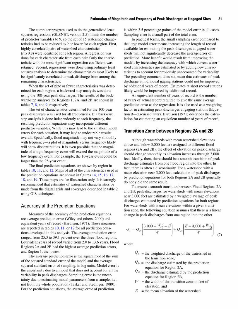
The computer program used to do the generalized least squares regressions (GLSNET, version 2.5), limits the number of predictor variables to 9, so the set of 15 watershed charac-teristics had to be reduced to 9 or fewer for each region. First, highly correlated pairs of watershed characteristics (r > 0.8) were identified for each region. A regression was done for each characteristic from each pair. Only the charac-teristic with the most significant regression coefficient was retained. Second, regressions were done using ordinary least squares analysis to determine the characteristics most likely to be significantly correlated to peak discharge from among the remaining characteristics.

When the set of nine or fewer characteristics was deter-mined for each region, a backward step analysis was done using the 100-year peak discharges. The results of the back-ward-step analyses for Regions 1, 2A, and 2B are shown in tables 7, 8, and 9, respectively.

The set of characteristics determined for the 100-year peak discharges was used for all frequencies. If a backward step analysis is done independently at each frequency, the resulting prediction equations may incorporate different predictor variables. While this may lead to the smallest model errors for each equation, it may lead to undesirable results overall. Specifically, flood magnitude may not vary smoothly with frequency—a plot of magnitude versus frequency likely will show discontinuities. It is even possible that the magni-tude of a high frequency event will exceed the magnitude of a low frequency event. For example, the 10-year event could be larger than the 25-year event.

The final prediction equations are shown by region in tables 10, 11, and 12. Maps of all of the characteristics used in the prediction equations are shown in figures 14, 15, 16, 17, 18, and 19. These maps are for illustration only. It is strongly recommended that estimates of watershed characteristics be made from the digital grids and coverages described in table 2 using GIS techniques.

Accuracy of the Prediction EquationsMeasures of the accuracy of the prediction equations

are average prediction error (Wiley and others, 2000) and equivalent years of record (Hardison, 1971). These measures are reported in tables 10, 11, or 12 for all prediction equa-tions developed in this analysis. The average prediction error ranged from 25.3 to 39.1 percent over the three flood regions. Equivalent years of record varied from 2.0 to 13.6 years. Flood Regions 2A and 2B had the highest average prediction errors, and Region 1, the lowest.

The average prediction error is the square root of the sum of the squared standard error of the model and the average squared standard error of sampling, in log units. Model error is the uncertainty due to a model that does not account for all the variability in peak discharges. Sampling error is the uncer-tainty due to estimating model parameters from a sample, i.e., not from the whole population (Tasker and Stedinger, 1989). For the prediction equations, the average error of prediction

is within 3.5 percentage points of the model error in all cases. Sampling error is a small part of the total error.

In practical terms, the small sampling error compared to the large model error means increasing the length of record available for estimating the peak discharges at gaged water-sheds will not significantly decrease the average error of prediction. More benefit would result from improving the models by increasing the accuracy with which current water-shed characteristics are estimated or by adding new charac-teristics to account for previously unaccounted for variability. The preceding comment does not mean that estimates of peak discharge at individual gaging stations could not be improved by additional years of record. Estimates at short record stations likely would be improved by additional record.

An equivalent number of years of record is the number of years of actual record required to give the same average prediction error as the regression. It is also used as a weighting factor in estimating peak discharges at gaging stations (Equa-tion 9—discussed later). Hardison (1971) describes the calcu-lation for estimating an equivalent number of years of record.

Transition Zone between Regions �A and �B

Although watersheds with mean watershed elevations above and below 3,000 feet are assigned to different flood regions (2A and 2B), the effect of elevation on peak discharge should change smoothly as elevation increases through 3,000 feet. Ideally, then, there should be a smooth transition of peak discharge estimates from one flood region into the other. In fact, there is often a discontinuity. For a watershed with a mean elevation near 3,000 feet, calculation of peak discharges by prediction equations for both Regions 2A and 2B generally do not yield the same result.

To ensure a smooth transition between Flood Regions 2A and 2B, peak discharges for watersheds with mean elevations near 3,000 feet are estimated by a weighted average of peak discharges estimated by prediction equations for both regions. For watersheds with mean elevations within a given transi-tion zone, the following equation assumes that there is a linear change in peak discharges from one region into the other.

T b aQ Q

W E

WQ

E W

W=

+ -æ

è

ççççç

ö

ø

÷÷÷÷÷+

- +æ

è

ççççç

ö

ø

÷÷÷2 2

3 000 2 3 000 2, ,÷÷÷

(7)

where

TQ = the weighted discharge of the watershed in the transition zone,

2aQ = the discharge estimated by the prediction equation for Region 2A,

2bQ = the discharge estimated by the prediction equation for Region 2B,

W = the width of the transition zone in feet of elevation, and

E = the mean elevation of the watershed.

Estimation of Magnitude and Frequency of Peak Discharges at Ungaged Sites �1

��

Estimation of Peak Discharges for Rural, Unregulated Stream

s in Western Oregon

Table �. Backward-step generalized least-squares regression analysis for 100-year peak discharges for Region 1, coastal watersheds.[Variables: All variables are log-transformed. Area, drainage area, in square miles; Slope, mean watershed slope, in degrees; Jul P, mean July precipitation, in inches; I24-2, 2-year 24-hour precipitation intensity, in inches; Mx Jan T, mean maximum January temperature, in degrees Fahrenheit; Mx Jul T, mean maximum July temperature, in degrees Fahrenheit; Soil C, soil storage capacity, in inches; Soil P, soil permeability, in inches per hour; Soil D, soil depth, in inches; --, variable removed. Selected model is indicated by the shaded area]

Predictor Variable

Step

a b c d e f g h i

Table values represent the probability that the coefficient for the predictor variable is not significantly different from zero.

Area 0.000 0.000 0.000 0.000 0.000 0.000 0.000 0.000 0.000

Slope 0.537 0.725 ----- ----- ----- ----- ----- ----- -----

Jul P 0.167 0.205 0.222 ----- ----- ----- ----- ----- -----

I24-2. 0.000 0.000 0.000 0.000 0.000 0.000 0.000 0.000 -----

Mx Jan T 0.254 0.232 0.194 0.020 0.009 ----- ----- ----- -----

Mx Jul T 0.033 0.040 0.038 0.092 ----- ----- ----- ----- -----

Soil C 0.007 0.007 0.004 0.002 0.007 0.013 ----- ----- -----

Soil P 0.002 0.001 0.001 0.001 0.002 0.002 0.013 ----- -----

Soil D 0.541 ----- ----- ----- ----- ----- ----- ----- -----

Model error, in log units 0.013013 0.012895 0.012732 0.012828 0.013179 0.014355 0.015489 0.016724 0.024422

Model error, in percent 26.7 26.6 26.4 26.5 26.9 28.1 29.3 30.5 37.2

Sampling error, in percent 13.2 12.6 12.0 11.2 10.7 10.1 9.5 8.9 8.6

Prediction error, in percent 30.0 29.6 29.2 29.0 29.1 30.0 30.9 31.8 38.3

Equivalent years of record 7.5 7.7 7.9 8.0 7.9 7.5 7.1 6.7 4.7

Estim

ation of Magnitude and Frequency of Peak Discharges at Ungaged Sites

��Table �. Backward-step generalized least-squares regression analysis for 100-year peak discharges for Region 2A, western interior watersheds with mean elevations greater than 3,000 feet.[Variables: All variables are log-transformed. Area, drainage area, in square miles; Slope, mean watershed slope, in degrees; Elev, mean watershed elevation, in feet; I24-2, 2-year 24-hour precipitation intensity, in inches; Jul P, mean July precipitation, in inches; Mn Jan T, mean minimum January temperature, in degrees Fahrenheit; Mx Jan T, mean maximum January temperature, in degrees Fahrenheit; Soil P, soil permeability, in inches per hour; Soil D, soil depth, in inches; --, variable removed Selected model is indicated by the shaded area]

Predictor Variable

Step

a b c d e f g h i


Area 0.000 0.000 0.000 0.000 0.000 0.000 0.000 0.000 0.000

Slope 0.000 0.000 0.000 0.000 0.000 0.000 0.000 0.000 --

Elev 0.425 0.373 0.359 0.335 -- -- -- -- --

I24-2 0.001 0.001 0.000 0.000 0.000 0.000 0.000 -- --

Jul P 0.926 0.916 -- -- -- -- -- -- --

Mn Jan T 0.001 0.000 0.000 0.000 0.000 0.000 -- -- --

Mx Jan T 0.045 0.028 0.018 0.014 0.008 -- --- -- --

Soil P 0.931 0.914 0.885 -- -- -- -- -- --

Soil D 0.989 -- -- -- -- -- -- -- --






��


s in Western Oregon

Table �. Backward-step generalized least-squares regression analysis for 100-year peak discharges for Region 2b, western interior watersheds with mean elevations less than 3,000 feet.[Variables: All variables are log-transformed. Area, drainage area, in square miles; Slope, mean watershed slope, in degrees; I24-2, 2-year 24-hour precipitation intensity, in inches; Jul P, mean July precipitation, in inches; Mx Jan T, mean maximum January temperature, in degrees Fahrenheit; Mx Jul T, mean maximum July temperature, in degrees Fahrenheit; Soil P, soil permeability, in inches per hour; Soil D, soil depth, in inches; Soil C, soil storage capacity, in inches; --, variable removed. Selected model is indicated by the shaded area]

Predictor Variable

Step

a b c d e f g h i


Area 0.000 0.000 0.000 0.000 0.000 0.000 0.000 0.000 0.000

Slope 0.000 0.000 0.000 0.000 0.000 0.000 0.000 0.000 --

I24-2 0.003 0.003 0.004 0.006 0.005 0.001 0.001 -- --

Jul P 0.153 0.179 0.238 0.332 0.313 -- --- -- --

Mx Jan T 0.344 0.367 0.354 -- -- -- -- -- --

Mx Jul T 0.601 0.496 -- -- -- -- -- -- --

Soil P 0.618 -- -- -- -- -- -- -- --

Soil D 0.050 0.043 0.029 0.035 0.038 0.066 -- -- --

Soil C 0.492 0.412 0.499 0.655 -- -- -- -- --






Estim

ation of Magnitude and Frequency of Peak Discharges at Ungaged Sites

��Table 10. Prediction equations for estimating peak discharges for ungaged watersheds in Region 1, coastal watersheds.

[Variables: Q(n), discharge in cubic feet per second for the n-year recurrence interval; Area, drainage area, in square miles; I24-2, 2-year 24-hour precipitation intensity, in inches; MxJanT, mean maximum January temperature, in degrees Fahrenheit; Soil C, soil storage capacity, in inches; Soil P, soil permeability, in inches per hour]

Prediction equation

Percent standard error of

the model, in percent

Average standard error of

sampling, in percent

Average prediction

error, in percent

Average equivalent

years of record

Q(2) = 0.05056Area0.9489 I24-21.360MxJanT1.280 Soil C-0.4421Soil P-0.1576 25.5 8.19 26.8 2.4


Q(10) = 0.008041Area0.9324 I24-21.226 MxJanT1.926 Soil C-0.5267Soil P-0.2552 23.9 8.68 25.6 5.0

Q(25) = 0.005122Area0.9258 I24-21.179 MxJanT2.109 Soil C-0.5484Soil P-0.2888 24.8 9.44 26.6 6.4




��


s in Western Oregon

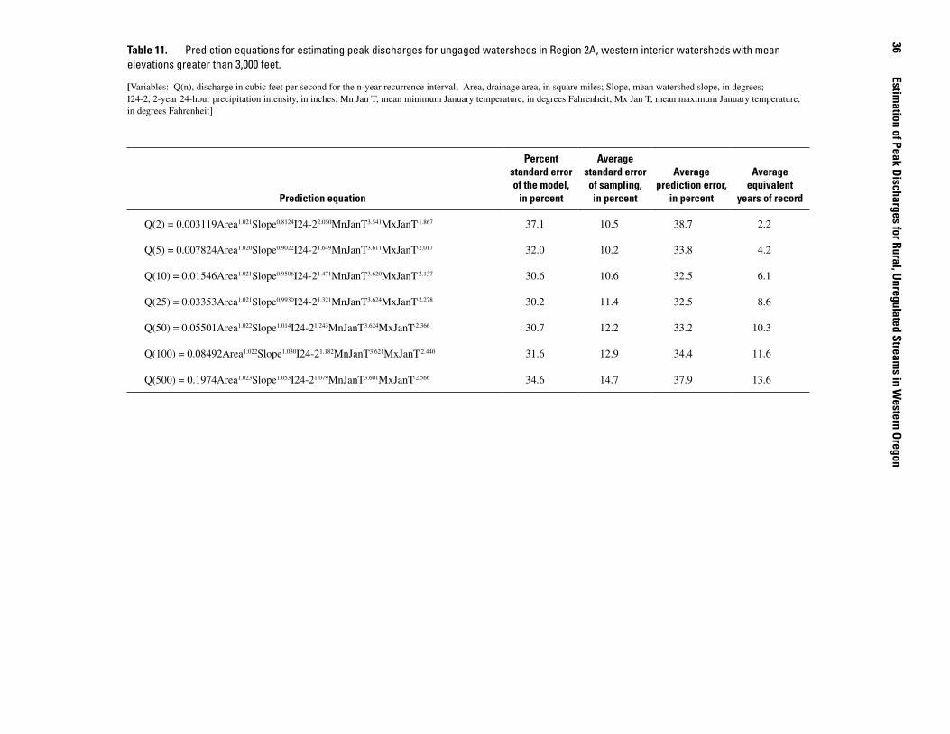
Table 11. Prediction equations for estimating peak discharges for ungaged watersheds in Region 2A, western interior watersheds with mean elevations greater than 3,000 feet.

[Variables: Q(n), discharge in cubic feet per second for the n-year recurrence interval; Area, drainage area, in square miles; Slope, mean watershed slope, in degrees; I24-2, 2-year 24-hour precipitation intensity, in inches; Mn Jan T, mean minimum January temperature, in degrees Fahrenheit; Mx Jan T, mean maximum January temperature, in degrees Fahrenheit]

Prediction equation

Percent standard error of the model,

in percent

Average standard error of sampling, in percent

Average prediction error,

in percent

Average equivalent

years of record

Q(2) = 0.003119Area1.021Slope0.8124I24-22.050MnJanT3.541MxJanT-1.867 37.1 10.5 38.7 2.2







Estimation of M

agnitude and Frequency of Peak Discharges at Ungaged Sites

��Table 1�. Prediction equations for estimating peak discharges for ungaged watersheds in Region 2B, western interior watersheds with mean elevations less than 3,000 feet.

[Variables: Q(n), discharge in cubic feet per second for the n-year recurrence interval; Area, drainage area, in square miles; Slope, mean watershed slope, in degrees; I24-2, 2-year 24-hour precipitation intensity, in inches]

Prediction Equation

Percent standard error of

the model, in percent

Average standard error

of sampling, in percent

Average prediction error,

in percent

Average equivalent years

of record

Q(2) = 9.136 Area0.9004Slope0.4695 I24-20.8481 31.9 6.53 32.6 2.0

Q(5) = 14.54 Area0.9042 Slope0.4735 I24-20.7355 31.6 6.85 32.4 2.8

Q(10) = 18.49 Area0.9064 Slope0.4688 I24-20.6937 32.0 7.28 33.0 3.6

Q(25) = 23.72 Area0.9086 Slope0.4615 I24-20.6578 33.0 7.90 34.1 4.8

Q(50) = 27.75 Area0.9101 Slope0.4559 I24-20.6390 34.0 8.37 35.1 5.5

Q(100) = 31.85 Area0.9114 Slope0.4501 I24-20.6252 35.0 8.83 36.2 6.2

Q(500) = 41.72 Area0.9141 Slope0.4365 I24-20.6059 37.7 9.87 39.1 7.5

Figure 1�. Areal distribution of slope.

Eugene

Ashland

Medford

Roseburg

Portland

Salem

Silet

z R

Klamath River

Rogue

Rive

r

Umpqua River

Illinois

River

NorthSantiam

River

North UmpquaRiver

South UmpquaRiver

Nehalem

River

Siuslaw

River

Will

amet

te

River

Desc

hute

s

GrantsPass

Sprague River

Will

iamso

n

River

Rive

r

CASC

ADE

RAN

GE

Eugene

Ashland

Medford

Roseburg

Portland

Salem

PACI

FIC

Silet

z R

Klamath River

Rogue

Rive

r

Umpqua River

Illinois

River

NorthSantiam

River

North UmpquaRiver

South UmpquaRiver

Nehalem

River

Siuslaw

River

COLUMBIA

RIVER

Will

amet

te

River

OCEA

N

Desc

hute

s

GrantsPass

Sprague River

Will

iamso

n

River

Rive

r

50 Miles

50 Kilometers

124°125° 122°123° 121°

42°

43°

44°

45°

46°

CASC

ADE

RAN

GE

0.00 – 3.22

3.23 – 8.25

8.26 – 14.0

14.1 – 20.3

20.4 – 27.3

27.4 – 35.6

35.7 – 84.2

EXPLANATION

Slope, in degrees

�� Estimation of Peak Discharges for Rural, Unregulated Streams in Western Oregon

Figure 1�. 2-year 24-hour precipitation intensity (1961–90). The isolines are superimposed on both a shaded relief map of elevation and the Geographic Information System grid of the 2-year 24-hour precipitation intensities on which the isolines are based. Darker areas represent higher precipitation intensities.

Eugene

Ashland

Medford

Roseburg

Portland

Salem

Silet

z R

Klamath River

Rogue

Rive

r

Umpqua River

River

NorthSantiam

River

North UmpquaRiver

South UmpquaRiver

Nehalem

River

Siuslaw

River

Will

amet

te

River

Desc

hute

s

GrantsPass

Sprague River

Will

iamso

n

River

Rive

r

CASC

ADE

RAN

GE

Eugene

Ashland

Medford

Roseburg

Portland

Salem

Silet

z R

Klamath River

Rogue

Rive

r

Umpqua River

River

NorthSantiam

River

North UmpquaRiver

South UmpquaRiver

Nehalem

River

Siuslaw

River

Will

amet

te

River

Desc

hute

s

GrantsPass

Sprague River

Will

iamso

n

River

Rive

r

CASC

ADE

RAN

GE

124°125° 122°123° 121°

42°

43°

44°

45°

46°

EXPLANATION

Two-year 24-hour precipitation intensity, in inches

1.01.5

2.03.04.05.06.0

7.0

PACI

FIC

COLUMBIA

RIVER

OCEA

N

50 Miles

50 Kilometers

Estimation of Magnitude and Frequency of Peak Discharges at Ungaged Sites ��

Figure 1�. Mean minimum January temperature (1961–90). The isolines are superimposed on both a shaded relief map of elevation and the Geographic Information System grid of the mean minimum January temperatures on which the isolines are based. Darker areas represent higher temperatures.

Eugene

Ashland

Medford

Roseburg

Portland

Salem

Silet

z R

Klamath River

Rogue

Rive

r

Umpqua River

Illinois

River

NorthSantiam

River

North UmpquaRiver

South UmpquaRiver

Nehalem

River

Siuslaw

River

Will

amet

te

River

Desc

hute

s

GrantsPass

Sprague River

Will

iamso

n

River

Rive

r

CASC

ADE

RAN

GE

Eugene

Ashland

Medford

Roseburg

Portland

Salem

Silet

z R

Klamath River

Rogue

Rive

r

Umpqua River

Illinois

River

NorthSantiam

River

North UmpquaRiver

South UmpquaRiver

Nehalem

River

Siuslaw

River

Will

amet

te

River

Desc

hute

s

GrantsPass

Sprague River

Will

iamso

n

River

Rive

r

CASC

ADE

RAN

GE

124°125° 122°123° 121°

42°

43°

44°

45°

46°

COLUMBIA

RIVER

PACI

FIC

OCEA

N

EXPLANATION

Mean minimum January temperature, in degrees Fahrenheit

1416182022242628303234363840

50 Miles

50 Kilometers

�0 Estimation of Peak Discharges for Rural, Unregulated Streams in Western Oregon

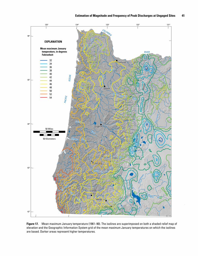
Figure 1�. Mean maximum January temperature (1961–90). The isolines are superimposed on both a shaded relief map of elevation and the Geographic Information System grid of the mean maximum January temperatures on which the isolines are based. Darker areas represent higher temperatures.

Eugene

Ashland

Medford

Roseburg

Portland

Salem

Silet

z R

Klamath River

Rogue

Rive

r

Umpqua River

Illinois

River

NorthSantiam

River

North UmpquaRiver

South UmpquaRiver

Nehalem

River

Siuslaw

River

Will

amet

te

River

Desc

hute

s

GrantsPass

Sprague River

Will

iamso

n

River

Rive

r

CASC

ADE

RAN

GE

Eugene

Ashland

Medford

Roseburg

Portland

Salem

Silet

z R

Klamath River

Rogue

Rive

r

Umpqua River

Illinois

River

NorthSantiam

River

North UmpquaRiver

South UmpquaRiver

Nehalem

River

Siuslaw

River

Will

amet

te

River

Desc

hute

s

GrantsPass

Sprague River

Will

iamso

n

River

Rive

r

CASC

ADE

RAN

GE

PACI

FIC

OCEA

N

COLUMBIA

RIVER

124°125° 122°123° 121°

42°

43°

44°

45°

46°

EXPLANATION

Mean maximum January temperature, in degrees Fahrenheit

323436384042444648505254

50 Miles

50 Kilometers

Estimation of Magnitude and Frequency of Peak Discharges at Ungaged Sites �1

Figure 1�. Areal distribution of soil storage capacity.

124°125° 122°123° 121°

42°

43°

44°

45°

46°

Eugene

Ashland

Medford

Roseburg

Portland

Salem

Silet

z R

Klamath River

Rogue

Rive

r

Umpqua River

Illinois

River

NorthSantiam

River

North UmpquaRiver

South UmpquaRiver

Nehalem

River

Siuslaw

River

Will

amet

te

River

Desc

hute

s

GrantsPass

Sprague River

Will

iamso

n

River

Rive

r

CASC

ADE

RAN

GE

Eugene

Ashland

Medford

Roseburg

Portland

Salem

PACI

FIC

Silet

z R

Klamath River

Rogue

Rive

r

Umpqua River

Illinois

River

NorthSantiam

River

North UmpquaRiver

South UmpquaRiver

Nehalem

River

Siuslaw

River

COLUMBIA

RIVER

Will

amet

te

River

OCEA

N

Desc

hute

s

GrantsPass

Sprague River

Will

iamso

n

River

Rive

r

CASC

ADE

RAN

GE

EXPLANATION

Soil capacity, in inches

0.00 – 0.03

0.04 – 0.08

0.09 – 0.11

0.12 – 0.14

0.15 – 0.17

0.18 – 0.26

0.27 – 0.41

50 Miles

50 Kilometers


Figure 1�. Areal distribution of soil permeability.

124°125° 122°123° 121°

42°

43°

44°

45°

46°

Eugene

Ashland

Medford

Roseburg

Portland

Salem

Silet

z R

Klamath River

Rogue

Rive

r

River

Illinois

River

NorthSantiam

River

North UmpquaRiver

South UmpquaRiver

Nehalem

River

Siuslaw

River

Will

amet

te

River

Desc

hute

s

GrantsPass

Sprague River

Will

iamso

n

River

Rive

r

CASC

ADE

RAN

GE

Eugene

Ashland

Medford

Roseburg

Portland

Salem

PACI

FIC

Silet

z R

Klamath River

Rogue

Rive

r

River

Illinois

River

NorthSantiam

River

North UmpquaRiver

South UmpquaRiver

Nehalem

River

Siuslaw

River

COLUMBIA

RIVER

Will

amet

te

RiverOC

EAN

Desc

hute

s

GrantsPass

Sprague River

Will

iamso

n

River

Rive

r

CASC

ADE

RAN

GE

EXPLANATION

Soil permeability, in inches per hour

0.00 – 0.92

0.93 – 1.88

1.89 – 3.00

3.01 – 4.63

4.64 – 7.21

7.22 – 10.9

11.0 – 20.0

50 Miles

50 Kilometers


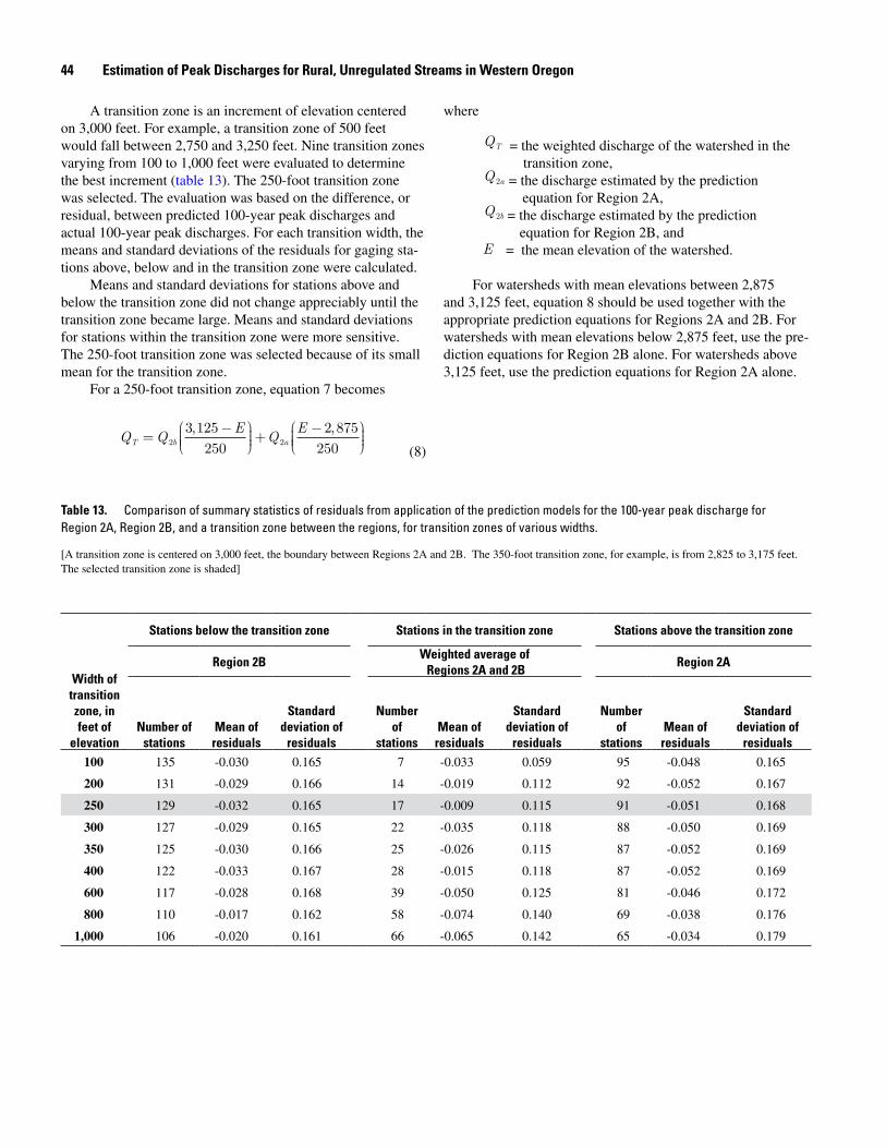
A transition zone is an increment of elevation centered on 3,000 feet. For example, a transition zone of 500 feet would fall between 2,750 and 3,250 feet. Nine transition zones varying from 100 to 1,000 feet were evaluated to determine the best increment (table 13). The 250-foot transition zone was selected. The evaluation was based on the difference, or residual, between predicted 100-year peak discharges and actual 100-year peak discharges. For each transition width, the means and standard deviations of the residuals for gaging sta-tions above, below and in the transition zone were calculated.

Means and standard deviations for stations above and below the transition zone did not change appreciably until the transition zone became large. Means and standard deviations for stations within the transition zone were more sensitive. The 250-foot transition zone was selected because of its small mean for the transition zone.

For a 250-foot transition zone, equation 7 becomes

T b aQ Q

EQ

E=

-æèççç

öø÷÷÷+

-æèççç

öø÷÷÷2 2

3 125250

2 875250

, ,

(8)

where

TQ = the weighted discharge of the watershed in the transition zone,

2aQ = the discharge estimated by the prediction equation for Region 2A,

2bQ = the discharge estimated by the prediction equation for Region 2B, and

E = the mean elevation of the watershed.

For watersheds with mean elevations between 2,875 and 3,125 feet, equation 8 should be used together with the appropriate prediction equations for Regions 2A and 2B. For watersheds with mean elevations below 2,875 feet, use the pre-diction equations for Region 2B alone. For watersheds above 3,125 feet, use the prediction equations for Region 2A alone.

Table 1�. Comparison of summary statistics of residuals from application of the prediction models for the 100-year peak discharge for Region 2A, Region 2B, and a transition zone between the regions, for transition zones of various widths.

[A transition zone is centered on 3,000 feet, the boundary between Regions 2A and 2B. The 350-foot transition zone, for example, is from 2,825 to 3,175 feet. The selected transition zone is shaded]

Width of transition zone, in feet of

elevation

Stations below the transition zone Stations in the transition zone Stations above the transition zone

Region �BWeighted average of Regions �A and �B

Region �A

Number of stations

Mean of residuals

Standard deviation of

residuals

Number of

stationsMean of residuals


residuals

Number of

stationsMean of residuals


residuals100 135 -0.030 0.165 7 -0.033 0.059 95 -0.048 0.165

200 131 -0.029 0.166 14 -0.019 0.112 92 -0.052 0.167

250 129 -0.032 0.165 17 -0.009 0.115 91 -0.051 0.168

300 127 -0.029 0.165 22 -0.035 0.118 88 -0.050 0.169

350 125 -0.030 0.166 25 -0.026 0.115 87 -0.052 0.169

400 122 -0.033 0.167 28 -0.015 0.118 87 -0.052 0.169

600 117 -0.028 0.168 39 -0.050 0.125 81 -0.046 0.172

800 110 -0.017 0.162 58 -0.074 0.140 69 -0.038 0.176

1,000 106 -0.020 0.161 66 -0.065 0.142 65 -0.034 0.179


Estimating Peak Discharges

The procedure for estimating peak discharges depends on whether the location of interest is gaged or ungaged, and if ungaged, whether it is near a gaged location on the same stream.

Gaged LocationsIf the watershed of interest is one of the gaged watersheds

listed in Appendix D, the frequency specific discharges may be read directly from the table. For Oregon gaging stations, the table gives three discharges at every frequency. The first discharge, designated S, is based on the systematic and histori-cal peak discharge record and is estimated by the guidelines of Bulletin 17B. The second, designated R, is estimated from the appropriate prediction equation given in table 10, 11, or 12. The third discharge, designated W, is a weighted average of the first two discharges (Wiley and others, 2000):

W

S RQQ N Q E

N E=

++

( )

( ) (9)

where

WQ = the weighted discharge, Qs = the discharge from the Pearson type III

distribution fitted to logarithms of the annual peak discharges at the gaging station,

RQ = the discharge estimated from the regional regression analysis,

N = the number of years of peak discharge record, and

E = the equivalent years of record.

All discharges are at a selected frequency and are in cubic feet per second.

For example, the weighted 100-year peak discharge at the gaging station McKenzie River near Vida, Oregon (14162500) is 75,400 cfs. The station (S) and prediction equation (R) esti-mated discharges are 70,800 cfs and 99,900 cfs, respectively.

Bulletin 17B (Interagency Advisory Committee on Water Data, 1982) recommends using the weighted discharge (W) as the estimate of peak discharge at the gaging station because its variance is less than the variance of either estimate (S or R). The weighting is discussed in detail in Appendix 8 of Bulletin 17B.

Limitations on the Use of Gaging Station Peak Dis-charges.—Streamflows at some of the gaging stations used in this report are now regulated. The peak discharges estimated from the frequency analysis and reported in Appendix D are based on peak discharges observed before the streams were regulated. The peak discharge estimates for each station repre-sent the stream in its unregulated state, not its current regulated

condition. The currently regulated stations are identified in Appendix D.

Ungaged LocationIf the watershed of interest is ungaged, the frequency-

specific discharge is calculated from the appropriate predic-tion equation given in table 10, 11, or 12. For example, for an ungaged watershed in Region 1, the 100-year peak discharge is given by

100Q = 0 9176 1 126 2 3250 003048 24 2Area I MxJanT−. . . .

0 3319SoilP − −. 00 5701.SoilC (10)

where

100Q = the 100-year peak discharge, in cubic feet per second,

Area = the drainage area of the watershed, in square miles,

I24 2− = the 2-year 24-hour precipitation intensity, in inches,

MxJanT = the mean maximum January temperature, in degrees Fahrenheit,

SoilP = the mean soil permeability, in inches per hour, and

SoilC = the mean soil storage capacity, in inches.

Lobster Creek, a tributary to Five Rivers, is an ungaged watershed in Region 1. The watershed above the mouth has a drainage area of 58.3 square miles, a 2-year 24-hour precipita-tion intensity of 3.69 inches, a mean maximum January tem-perature of 47.6 degrees Fahrenheit, a mean soil permeability of 2.51 inches per hour, and a mean soil storage capacity of 0.134 inches. Substituting these values into Equation 10 yields

Q100 = 0.003048 × 58.30.91763.691.12647.62.3252.51-0.33190.134-0.5701

100 10 200Q cfs= ,

Transition Zone between Regions 2A and 2BConsider Quartz Creek, a tributary of the McKenzie

River. The watershed at the mouth of Quartz Creek has a mean elevation of 2,960 feet—within the transition zone between Regions 2A and 2B. The estimated 100-year peak discharge for Region 2A is 7,690 cfs and for Region 2B, 8,380. Substi-tuting into Equation 8,

TQ =-æ

èççç

öø÷÷÷+

-æèççç

ö7 690

3 125 2 970250

8 3802 970 2 875

250,

, ,,

, ,øø÷÷÷


TQ cfs= 7 950,

Selected watershed characteristics for Quartz Creek are shown in table 14.

Table 1�. Selected characteristics for the ungaged watershed Quartz Creek at the mouth.

Watershed characteristic

Drainage area, in square miles 42.1

Mean watershed elevation, in feet 2,970

Mean watershed slope, in degrees 23.8

2-year 24-hour precipitation intensity, in inches

2.84

Mean minimum January temperature, in degrees Fahrenheit

31.0

Mean maximum January temperature in degrees Fahrenheit

44.3

Limitations on the Use of the Prediction EquationsThe prediction equations may be used to estimate peak

flows for any stream. However, the prediction equations do not account for reservoir operations, diversion, urbanization, or significant contributions from spring flow. Many streams are affected by these factors. In these cases, the estimates of peak flow represent a hypothetical condition of the watershed, not the actual condition.

Unless the user intends to predict peak discharges for the hypothetical condition of a watershed, the prediction equations should be used only on rural, unregulated streams and where streamflow arises primarily from storm runoff or snowmelt rather than spring flow. They should not be used where there are significant areas of impervious surface due to pavement or buildings, or where streams have been lined or diverted through culverts or artificial channels. They also should not be used for streams regulated by reservoirs, diversion, or large natural lakes. Also to be avoided are streams with large losses to ground water.

There are not many streams in western Oregon domi-nated by spring flow, but they do occur occasionally. They are most likely to be found in areas of young volcanic rock in the Cascade Range. Streams with large losses also occur in young volcanic rock in the Cascades and perhaps in coastal streams flowing over unconsolidated sand.

In all cases, hypothetical or not, the equations should not be used for watersheds that have characteristics that fall outside the range of characteristics of the watersheds used to develop the prediction equations. The ranges of characteristics for these watersheds are given in table 15.

Ungaged Location, near a Gaging Station on the Same Stream

If an ungaged watershed is on the same stream as a gaged watershed listed in this report, and the ungaged watershed has an area between 0.50 and 1.50 times the area of the gaged watershed, peak discharges at the ungaged site may be calcu-lated from the peak discharges at the gaged site by this equa-tion (Thomas and others, 1993; Sumioka and others, 1997):

u g

a

u

g

Q QA

A=

æèççç

öø÷÷÷

(11)

where

uQ = the estimated discharge for the ungaged watershed,

gQ = the weighted discharge (W) from Appendix D for

the gaging station,uA = the area of the ungaged watershed,gA = the area of the gaged watershed, and

a = the exponent of area from the prediction equations in table 10, 11, or 12.

All discharges are at a selected frequency and are in cubic feet per second. The exponent is from the prediction equation for the selected frequency.

Equation 11 should be used only if the gaged and ungaged watersheds have similar characteristics. If the water-sheds differ appreciably in topography, vegetative cover, or geology, the peak discharge estimates should be made by way of the appropriate prediction equations.

Consider the Applegate River, a tributary of the Rogue River. This stream, at its mouth, is ungaged, and peak dis-charges could be estimated by the prediction equations for Region 2A—the mean watershed elevation is greater than 3,000 feet. However, there is a gaging station, Applegate River at Wilderville (14369500), 7.6 miles upstream. Selected characteristics for the gaged and ungaged watersheds are given in table 16. The watersheds are similar and use of Equation 11 is appropriate.

From table 11 for the 100-year peak discharge for Region 2A, the area coefficient is 1.022. Taking the areas from table 16 and the 100-year peak discharge for the Applegate River at Wilderville from Appendix D, then making the substitutions into Equation 11,

uQ = ( )101 000

771

699

1 022

,

.

uQ cfs= 112 000,


Estimation of M

agnitude and Frequency of Peak Discharges at Ungaged Sites

��

Table 1�. Ranges of characteristics for the gaged watersheds used to develop the prediction equations, by region.

[--, characteristic not in equation]

RegionNumber of

stationsDrainage area, in square miles

Mean �-year ��-hour

precipitation intensity, in inches

Mean water-shed slope, in degrees

Mean minimum January

temperature, in degrees Fahrenheit

Mean maximum January

temperature, in degrees Fahrenheit

Mean soil storage

capacity, in inches

Mean soil permeability,

in inches per hour

1 91 0.28–673 2.52–5.79 -- -- 42.4–53.9 0.10–0.23 0.72–4.76

2A 107 0.22–3,940 1.72–4.34 6.24–28.0 20.5–34.0 33.9–47.3 -- --

2B 178 0.37–7,270 1.53–4.48 5.62–28.3 -- -- -- --

Table 1�. Selected characteristics for the ungaged watershed Applegate River at the mouth and for the gaged watershed Applegate River at Wilderville, Oregon (14369500).

Watershed characteristicUngaged watershed Gaged watershed

Applegate River at the mouth Applegate River at Wilderville (1��00)

Drainage area, in square miles 771 699

Mean watershed elevation, in feet 3,140 3,280

Mean watershed slope, in degrees 20.7 21.0

Mean 2-year 24-hour precipitation intensity, in inches 2.31 2.29

Mean minimum January temperature, in degrees Fahrenheit 28.6 28.3

Mean maximum January temperature, in degrees Fahrenheit 42.5 42.1

Mean soil depth, in inches 36.0 35.8


Making Estimates of Peak Discharge at the Oregon Water Resources Department Web Site

At the Oregon Water Resources Department Web site (http://www.wrd.state.or.us/), a user can make estimates of peak discharge magnitudes at the selected frequencies by one of four methods:

Selecting from among about 1,200 watersheds for which the physical characteristics are already known,

Manually entering the required watershed characteristics,

Submitting a user-delineated watershed, or

Using a utility on the Web site to autodelineate the water-shed.

Because of the inherent difficulties in independently esti-mating watershed characteristics, it is strongly recommended the user take advantage of options 1, 3, and 4 listed above rather than option 2. In all cases, a report detailing peak discharges and how they were determined for the specified watershed is returned to the user.

Selecting among already delineated watersheds (Option 1) is done onscreen using interactive maps. For manual input (Option 2), a form is provided. If the user supplies the water-shed delineation (Option 3), it must be submitted as a “shape file” in Oregon Lambert coordinates. A shape file is an open specification for a GIS theme developed by Environmental Systems Research Institute, Inc.

For Option 4, the user need only select a point on a stream where the magnitude of a specified peak discharge is desired. Selection of the point is done interactively from topo-graphic maps displayed onscreen. Nothing further is required from the user. Delineation of the watershed above the selected point, determination of the watershed characteristics, and calculation of the peak discharges are done automatically. The autodelineation program, however, does not account for the effects of reservoir operations, diversion or urbanization. Please refer to Oregon Water Resources Department’s Web site (http://www.wrd.state.or.us/surface_water/flood/index.shtml) for more information.

The user may also obtain, online, the peak discharge characteristics for the 376 gaging stations used in this study. In addition to the discharge magnitudes given in Appendix D of this report, the online version includes the 95 percent confidence intervals.

SummaryAn analysis of the magnitude and frequency of peak dis-

charges in western Oregon has been completed with financial assistance from the Federal Emergency Management Agency, the Oregon Department of Transportation, and the Associa-tion of Oregon Counties, and with the cooperation of the U.S.

1.

2.

3.

4.

Geological Survey. The study was undertaken to provide engi-neers and land managers with the information needed to make informed decisions about development in or near watercourses in the study area.

This report describes the results of an analysis of the peak discharges of rural streams in Oregon west of the Cascade crest. These results include (1) the magnitude of annual peak discharges for selected frequencies at 376 gaging stations, (2) generalized logarithmic skew coefficients for Oregon, and (3) sets of equations relating the magnitude of peak discharges at selected frequencies to physical and climatological watershed characteristics such as drainage area or mean January precipi-tation. There is a set of frequency specific prediction equations for each of three hydrologically homogeneous “flood regions” within western Oregon. The selected frequencies give the interval at which a peak discharge of given magnitude is likely to recur. The recurrence intervals are 2, 5, 10, 20, 25, 50, 100, and 500 years.

The logarithms of peak discharges at 376 streamflow gaging stations in western Oregon, southwestern Washington, and northwestern California were fitted to the Pearson Type III distribution. The parameters of the Pearson Type III distribu-tion were adjusted for the effects of high and low outliers, for historic peaks, for zero peaks, and for peaks below the gage threshold based on guidelines in Interagency Advisory Committee on Water Data’s Bulletin 17B. Station skew values also were adjusted by a “generalized” skew value based on the skews for long-term stations in the area.

The areal distribution of the generalized logarithmic skew coefficients of annual peak discharge for Oregon was deter-mined using GIS techniques. Generalized skew coefficients derived from the distribution were used to improve estimates of skew for short record gaging stations. The areal distribution is a GIS grid but is represented in this report as an isoline map. In practice, generalized skew coefficients are determined from the grid, not the isoline map. The grid is available on request ([email protected]).

A combination of regression techniques was used to derive the prediction equations. A preliminary analysis using ordinary least-squares regression was conducted to define flood regions of homogeneous hydrology and to determine which climatological and physical characteristics of the watersheds would be most useful in the prediction equations. The final prediction equations were derived using generalized least-squares regression. The computer model, GLSNET (ver-sion 2.5), developed by the U.S. Geological Survey was used to do the generalized least-squares regression analysis. Aver-age standard error of prediction for the equations for the three flood regions ranged from 25.3 to 39.1 percent. Equivalent years of record varied from 2.0 to 13.6 years.

The prediction equation may be used to estimate peak flows for any stream. However, the prediction equations do not account for reservoir operations, diversion or urbanization. Many streams are affected by these factors. In these cases, the estimates of peak flow represent a hypothetical condition of the watershed, not the actual condition.

http://www.wrd.state.or.us/

http://www.wrd.state.or.us/surface_water/flood/index.shtml

http://www.wrd.state.or.us/surface_water/flood/index.shtml

mailto:[email protected]

Use of the prediction equations requires estimates of sev-eral physical and climatological characteristics of the water-shed in question. Because the watershed characteristics can be difficult to estimate, the Oregon Water Resources Department has developed an interactive utility, available on its Web site, to facilitate the use of the equations. The user need only select a site on a stream from an onscreen interactive map and the magnitude of floods at various frequencies will be reported for that location. To use the interactive utility, go to http://www.wrd.state.or.us/OWRD/SW/peak_flow.shtml

References

Advisory Committee on Water Information, 2002, Bulletin 17–B flood frequency guidelines—Frequently asked ques-tions: U.S. Geological Survey, http://water.usgs.gov/wicp/acwi/hydrology/Frequency/B17bFAQ.html, accessed Febru-ary 2003.

Baldwin, E.M., 1981, Oregon geology, Third edition: Dubuque, Iowa, Kendall/Hunt Publishing Company, 170 p.

Brands, M.D., 1947, Flood runoff in the Willamette Val-ley, Oregon: U.S. Geological Survey Water-Supply Paper 968–A, 59 p.

Campbell, A.J., Sidle, R.C., and Froehlich, H.A., 1982, Pre-diction of peak flows for culvert design on small water-sheds in Oregon: Corvallis, Oregon State University Water Resources Research Institute, 96 p.

Crippen, J.F., 1978, Composite log-Pearson Type III fre-quency-magnitude curve of annual floods: U.S. Geological Survey Open-File Report 78–352, 5 p.

Daly, C., Taylor, G.H., and Gibson, W.P., 1997, The PRISM approach to mapping precipitation and temperature, in Reprints of 10th Conference on Applied Climatology, Reno, Nevada: American Meteorological Society, p. 10–12.

Dicken, S.N., 1965, Oregon geography, fourth edition: Ann Arbor, Michigan, Edwards Brothers, Inc., 104 p.

Gannett, M.W., Lite, K.E., Morgan, D.S., and Collins, C.A., 2000, Ground-water hydrology of the upper Deschutes Basin, Oregon: U.S. Geological Survey Water-Resources Investigations Report 00–4162, 77 p.

Hardison, C.H., 1971, Prediction error of regression estimates of streamflow characteristics at ungaged sites: U.S. Geo-logical Survey Professional Paper 750–C, p. C228-C236.

Harris, D.D., Hubbard, L.L., and Hubbard, L.E., 1979, Mag-nitude and frequency of floods in western Oregon: U.S. Geological Survey Open-File Report 79–553, 29 p.

Hazen, A., 1930, Flood Flows: John Wiley and Sons, Inc., New York.

Hofmann, W., and Rantz, S.E., 1963, Floods of December 1955 to January 1956 in the far western States, Part 1—Description: U.S. Geological Survey Water-Supply Paper 1650–A, 156 p.

Hubbard, L.L., 1991, Oregon floods and droughts, in National Water Summary 1988-89: U.S. Geological Survey Water-Supply Paper 2375, p. 459–466.

Hubbard, L.L.,1996, Floods of January 9-11, 1990, in north-western Oregon and southwestern Washington, in Summary of floods in the United States during 1990 and 1991: U.S. Geological Survey Water-Supply Paper 2474, p. 11–16.

Hulsing, H., and Kallio, N.A., 1964, Pacific slope basins in Oregon and lower Columbia River basin, part 14 of Mag-nitude and frequency of floods in the United States: U.S. Geological Survey Water-Supply Paper 1689, 320 p.

Interagency Advisory Committee on Water Data, 1982, Guide-lines for determining flood flow frequency—Bulletin 17B of the Hydrology Subcommittee: Reston, Virginia, U.S. Geological Survey, Office of Water Data Coordination, 28 p.

Laenen, Antonius, 1980, Magnitude and frequency of storm runoff as related to urbanization in the Portland, Oregon-Vancouver, Washington area: U.S. Geological Survey Open-File Report 80–689.

Laenen, Antonius, 1983, Storm runoff as related to urbaniza-tion based on data collected in Salem and Portland and gen-eralized for the Willamette Valley, Oregon: U.S. Geological Survey Water-Resources Investigations Report 83-4143.

Lumia, R., and Baevsky, Y., 2000, Development of a contour map showing generalized skew coefficients of annual peak discharges of rural, unregulated streams in New York, excluding Long Island: U.S. Geological Survey Water-Resources Investigations Report 00–4022, 11p.

Lystrom, D.J., 1970, Evaluation of the streamflow-data pro-gram in Oregon: U.S. Geological Survey Open-File Report, 28 p.

National Cartography and Geospatial Center, 1994, State soil geographic (STATSGO) database (1:250,000 scale): U.S. Department of Agriculture, Natural Resources Conservation Service, http://www.ncgc.nrcs.usda.gov/products/datasets/statsgo/, accessed July 1995.

National Center for Earth Resources Observation & Science, 1999, National elevation dataset, one arc-sec resolution: U.S. Geological Survey, http://edc.usgs.gov, accessed March 2005.

Summary ��

http://www.wrd.state.or.us/OWRD/SW/peak_flow.shtml

http://www.wrd.state.or.us/OWRD/SW/peak_flow.shtml

http://water.usgs.gov/wicp/acwi/hydrology/Frequency/B17bFAQ.html

http://water.usgs.gov/wicp/acwi/hydrology/Frequency/B17bFAQ.html

http://www.ncgc.nrcs.usda.gov/products/datasets/statsgo/

http://www.ncgc.nrcs.usda.gov/products/datasets/statsgo/

http://edc.usgs.gov

�0 Estimation of Peak Discharges for Rural, Unregulated Streams in Western Oregon

Oregon Water Resources Department, 1971, Regionalized flood frequency data for Oregon: Salem, Oregon, 33 p.

Paulsen, C.G., 1953, Floods of southwestern Oregon, north-western California: U.S Geological Survey Water-Supply Paper 1137–E, 191 p.

Rantz, S.E., 1959, Floods of January 1953 in western Oregon and northwestern California: U.S. Geological Survey Water-Supply Paper 1320–D, 19 p.

Riggs, H.C., 1968, Some statistical tools in hydrology: U.S. Geological Survey Techniques of Water Resources Investi-gations, book 4, chapter A1, 39 p.

Riggs, H.C., 1973, Regional analysis of streamflow char-acteristics: U.S. Geological Survey Techniques of Water Resources Investigations, book 4, chapter B3, 15 p.

Sauer, V.B., Thomas, Jr., W.O., Stricker, V.A., and Wilson, K.V., 1983, Flood characteristics of urban watersheds in the United States: U.S. Geological Survey Water-Supply Paper 2207, 37 p.

Sauer, V.B, 2002, Urban flood frequency estimating tech-niques in The national flood frequency program, version 3: A computer program for estimating magnitude and fre-quency of floods at ungaged sites: U.S. Geological Survey Water-Resources Investigations Report 02–4168, p. 8–10.

Sumioka, D.L., Kresch, D.L., and Kasnick, K.D., 1997, Magnitude and frequency of floods in Washington: U.S. Geological Survey Water-Resources Investigations Report 97–4277, 91 p.

Tasker, G.D., Eychaner, J.H., and Stedinger, J.R., 1986, Appli-cation of generalized least-squares in regional hydrologic regression analysis in Subitsky, Seymour, ed., Selected papers in the hydrologic sciences, 1986: U.S. Geological Survey Water-Supply Paper 2310, p. 107–115.

Tasker, G.D., and Stedinger, J.R., 1989, An operational GLS model for hydrologic regression: Journal of Hydrology, v. 111, p. 361–375.

Taylor, G.H. and Hatton, R.R., 1999, The Oregon weather book, a state of extremes: Corvallis, Oregon State Univer-sity Press, 242 p.

Thomas, B.E., Hjalmerson, H.W., and Waltemeyer, S.D., 1993, Methods for estimating magnitude and frequency of floods in the southwestern United States: U.S. Geological Survey Open-File Report 93–419, 211 p.

Thomas, D.M., and Benson, M.A., 1969, Generalization of streamflow characteristics from drainage watershed charac-teristics: U.S. Geological Survey Open-File Report, 45 p.

U.S. Geological Survey, 2000, GLSNET—Regional hydro-logic regression and network analysis using generalized least squares (Version 2.5): http://water.usgs.gov/software/glsnet.html, last modified 9/29/1997, accessed August 2002.

U.S. Water Resources Council, 1977, Guidelines for determin-ing flood flow frequency: Washington, D.C., U.S. Water Resources Council Bulletin 17A, 26 p.

Waananen, A.O., Harris, D.D., and Williams, R.C., 1971, Floods of December 1964 and January 1965 in the far west-ern United States, Part 1—Description: U.S. Geological Survey Water-Supply Paper 1866–A, 265 p.

Wiley, J.B., Atkins, Jr., J.T., and Tasker, G.D., 2000, Estimat-ing magnitude and frequency of peak discharges for rural, unregulated streams in West Virginia: U.S. Geological Survey Water-Resources Investigations Report 00–4080, 93 p.

http://water.usgs.gov/soft/glsnet.html

http://water.usgs.gov/software/glsnet.html

transition zone between regions a and b - usgs · highly correlated pairs of watershed...

Documents