transitional growth paths in developing economies...transitional growth paths in developing...

��

��

Transitional Growth Paths

in Developing Economies

��

��

��

��

Transitional growth paths in developing economies

Peter E. Robertson*

University of New South Wales.

7 May, 1997

This paper develops model of growth in an economy where the capital stock isrationed across labour inputs, as in the dual, or segmented, labour marketliterature on developing economies. In this economy, the increased use oflabour in the formal sectors can sustain high marginal and average products ofcapital and high growth rates for periods of 15-30 years. This provides aninteresting insight into the current growth and convergence debate. The modelis shown to overcome the empirical problems of the standard Ramsey growthmodel and also avoids some recent criticisms of endogenous growth models.

Key words: growth, development, endogenous growth, dual labour markets,

convergence.

JEL Classification; OO, O1, O3, D9

* I would like to thank Kevin Fox, Geoff Kingston, Murray Kemp, Jim Melvin, Anu

Rammohan, Allan Würtz and Minxian Yang and seminar participants at the ThirdAustralian Macroeconomics Workshop, and the 23rd Australian Conference of Economists.Special debt is owed to Rick Harris. All errors and omissions are my own.

Correspondence to Peter Robertson, School of Economics, University of New South Wales,Sydney, 2052, Australia.Email: [email protected],Internet: http://www.fce.unsw.edu.au/econ/robertson.htm

2

1. Introduction

In the last half of this century we have witnessed the dramatic economic

success of Japan, South Korea and other newly industrialising economies

(NIEs) and the equally dramatic economic failure of many countries,

especially in Africa and South Asia. These differences are well known and

illustrated in Figures 1. Japan and South Korea, for example, achieved average

growth rates of above five percent over twenty year periods, compared to

average growth rates below two percent in much of the developing world. In

order to design policies which can assist growth and development in low

income economies, it is necessary to understand the causes of the rapid growth

in the successful developing economies.

(Fig. 1 here)

Mankiw, Romer and Weil (1992), Barro and Sala-i-Martin (1992, 1995), Sala-

i-Martin, (1994) and Mankiw (1995) argue that the standard Ramsey growth

model, with diminishing returns to capital, explains why growth rates should

be high in low income economies.1 A relatively small stock of capital results

in high average and marginal products of capital. This causes a high, but

monotonically falling, growth rate which, the authors suggest, accounts for the

performance of the NIEs. King and Rebelo (1993) show, however, that the

transition paths in this model, are too short, display too little persistence, and

imply an initial growth rate and marginal product of capital that is too high,

(King and Rebelo, 1993 p. 929).2

1 The standard Ramsey growth model is discussed, for example, in Blanchard and

Fisher (1989) or Barro and Sala-i-Martin (1995). See also Solow (1956) and Swan (1956),who pioneered the neoclassical growth model.

2 For example, they argue that to explain the Japanese economic miracle in the traditionalgrowth model requires a marginal product of capital of 500% in 1950. King and Rebelo’scriticisms apply even if human capital is included in the aggregate capital stock, which isthe remedy suggested by Mankiw, Romer and Weil (1992), Mankiw (1995) pp. 290-291,and Barro and Sala-i-Martin (1995) pp. 80-87. In this case the higher aggregate capitalshare implies transitional implies unrealistically high long run investment rates. Furtherdoubt has been shed on the empirical reliance of the Mankiw et al (1992) model by Caselli

3

Along with Romer (1986, 1990) and Lucas (1988, 1993), King and

Rebelo (1993) therefore contend that an accurate understanding of growth

miracles depends primarily on an understanding of the process of productivity

growth, or on conditions where the production function does not exhibit a

diminishing marginal product of capital. There are however, several

difficulties with these endogenous growth models. First many predict

increasing long run growth rates, whereas there is no strong evidence of this in

time series data, (Jones 1995, Ben–David and Papell, 1995). Second, many

also predict high levels of productivity growth in rapid growth economies.

Recent, growth accounting studies of the East Asian NIEs, however, do not

support this prediction, (Young 1994, 1995, Kim and Lau 1993, and Pilat

1994).3

The purpose of this paper is to describe an important aspect of growth in

developing economies, which has hitherto been overlooked in this debate. If

the economy has a dual or segmented, labour market structure then a

significant part of the growth process may be due to high rates of capital

accumulation, without unusually high rates of technology change. This is

because diminishing returns to capital may be offset by the increased

employment of labour from low wage informal sectors of the economy, which

does not otherwise have access to modern sector capital. In this case the

marginal product of capital, the savings rate and the growth rate are relatively

constant over the early stages of development. It is shown that the modified

model generates high and persistent growth rates and realistic levels of

investment and the marginal product of capital. Thus rapid accumulation can

occur in the medium term without high rates of technology change.

et al (1996). They argue that after correcting for mis specification bias the human capitalaugmented growth model also implies unrealistically fast transitions.

3 This results are supported by Havrylyshyn, (1992), who shows that developing countrieshave typically been found to have lower productivity residuals than the developed countries.

4

The paper is organised as follows. Section 2 briefly discusses the nature of

labour markets in developing countries. It then incorporates the dual, or

segmented, labour market hypothesis into the standard Ramsey growth model.

In section 3 the transition properties of the dual labour market model are

discussed and section 4 assesses the model using numerical simulations,

calibrated to Japanese and South Korean post war data. Section 5 concludes.

2. Growth, convergence and development with dual labour markets.

Dual labour market theory was pioneered by Lewis (1954) and developed into

formal models of development by Sen (1966), Ranis and Fei (1961),

Marglin (1984), Dixit (1968), Stern (1971), Minami (1973) among others. In

these models, growth in the modern sector of a developing economy induced

labour migration from the less developed rural regions. Harris and

Todaro (1970), Fields (1975), Mazumdar (1985) and Kannapan (1985)

extended this idea in the theory of segmented labour markets – the existence

of different real wage rates for labour of similar skills. The common element

in all of these theories is that entry to the high productivity, or formal, sector is

rationed. Thus an expansion of the formal sector labour demand results in an

increase in labour supply. Informal sector output declines, but by less than the

increase in formal sector output.

The theory of segmented labour markets in developing countries is not

uncontroversial.4 Nevertheless empirical evidence shows the presence of

urban-rural wage gaps for low skilled labour, Squire (1981), wage gaps

4 For discussion of microeconomic models of labour market conditions in LDC’s see

Gregory (1980), Basu (1984), Mazumdar (1983), Stiglitz (1988), Rosensweig (1988),Williamson (1988), Dasgupta (1993), and Freeman (1993). The segmented labour markettheory should also be distinguished from the “surplus labour” hypothesis which maintainsthat output in the informal sector does not fall as labour is withdrawn, Dasgupta (1993). Theclaim of the segmented labour market hypothesis is that labour’s marginal contribution tooutput in the formal sector is larger than the decline in the informal sector.

5

according to factory size, Mazumdar (1979, 1985), and rationed access to

education and capital markets resulting in high rents to those with skills,

Sundrum (1990), Williamson (1993). There are also significant migrant labour

supply responses to these wage gaps, (Ghatak, Levine and Wheatley-Price,

1996).5 The dual nature of labour markets has featured heavily in many

descriptive accounts of the development in Japan (Fei, Ohkawa and Ranis,

1985, Minami, 1973, 1986), and other NIEs, (Amsden, 1989 Bai, 1982,

Fields, 1994, Ranis, 1995). Moreover, the role of improved resource allocation

in general for the East Asian NIEs has been stressed by Olson (1996) and The

World Bank (1993). Thus, the segmented or dual labour market has received

considerable attention in the development literature. In view of this the

remainder of this paper is concerned only with investigating the implications

of the dual labour market hypothesis for the pattern of growth.

Assume that the economy has two sectors, informal and formal, and labour in

the formal receives a constant wage, w which is greater than the informal

wage rate. This follows earlier growth models with dual labour markets and

generates job rationing in the formal sector for sufficiently low capital stocks.6

Also following earlier growth models, we simplify matters by considering the

formal sector only. The equations for capital accumulation and output are;

5 While wage gaps exists, they are not ubiquitous and may vary substantially. Recent country

studies supporting the segmented labour market hypothesis for developing countriesinclude; Marcouiller, Ruiz de Castila and Woodruff (1995), who report formal to informalwage ratios of 1.5 - 2 in El Salvador and Peru, but find no segmentation in Mexico; Beckar,Hamer and Morrison (1994) who site urban to rural wage ratios of 5-10 in some Africaneconomies and Ranis (1995) who reports ratios of approximately 1.5 - 2.5 in Taiwan andSouth Korea. See also Basch and Paredes–Molina (1996), and Magnac (1991). SeeRosensweig (1988) for a critique of the measurement problems involved.

6 The most commonly suggested cause of segmented labour markets is efficiency wages, seeLeibenstein, (1963), Bliss and Stern (1978), and Mazumdar (1983) and Dasgupta (1993).Fields and Wan (1989) present evidence that the institutions have been an important part ofwage setting in Latin American. The difference between this model and models byDixit (1968) and Stern (1972) and Marglin (1984) is that they considered the intertemporaloptimal allocation of labour in the context of a normative planning problem, and restrictedsavings to be from profits, and not wages. See also Solow’s (1956) discussion of real wagerigidity.

6

�( ) ( ) ( ) ( )k t y t c t nk t= − − , (1)

y t A t f k t ,l t( ) ( ) ( ( ) ( ))= fi > 0, fii <0, i = 1, 2, (2)

N t N e0nt( ) = , (3)

where N(t) is the labour force and l(t) ≡ L(t)/N(t) is the ratio workers employed

in the formal sector to the total labour force. The remaining 1-l(t) workers are

in the informal sector. A(t) represents the level of technology, k(t) is capital

per worker, y(t) is output of the formal sector per worker and f ( )⋅ is assumed

to be homogeneous of degree one. It will useful to define all t such that

l(t) < 1, as phase 1 and all t such that l(t) = 1, as phase 2.

Firms in the formal sector are assumed to maximise current profits, π(t),

taking prices as given. Thus the representative firm maximises,

π( ) = ( ) ( ( ), ( )) - ( ) ( ) - ( ) ( )t A t f k t l t w t l t r t k t , (4a)

subject to the constraint that,

w t w( ) ≥ . (4b)

Dropping time subscripts, the necessary first order conditions for profits

maximisation are:

A f2 (k, l) = w, (5a)

A f1 (k, l) = r . (5b)

If the constraint (4b) holds with equality, then firms adjust their labour inputs,

l. That is, if Af2 (k, 1) < w , then,

7

Af2 (k, l) = w . (6)

Because the production function is homogeneous of degree one, f2(k, l) is

homogeneous of degree zero and can be written as a function of the ratio k/l.

Thus the value of l which solves equation is (6), �l , is linear in k,

�l = �l (A, w )k.7

The optimal choice of labour per worker can be expressed as, �l = min(�l , 1).

In phase 1, �l = �l and y = f(k, �l ) ≡ g(A, w )k. Output must also be a linear

function of the capital stock in phase 1.8 In general, output may be expressed

as,

�y =A f(k, �l ) ≡ min [g(A, w )k, f(k, 1)]. (7)

The representative consumer in the formal sector is assumed to maximise

utility subject to (1), (3) and (7). The intertemporal utility function depends on

consumption per person and the number of people in the formal sector,

U c l u c l e dtt

t( , ) ( , )==

−∞∫ 0

ρ . To solve the consumer’s optimisation problem the

current value Hamiltonian is formed.

H(k, c, l, λ) = N u(c, l) + λ[Af(k, �l ) - nk - c ]. (8)

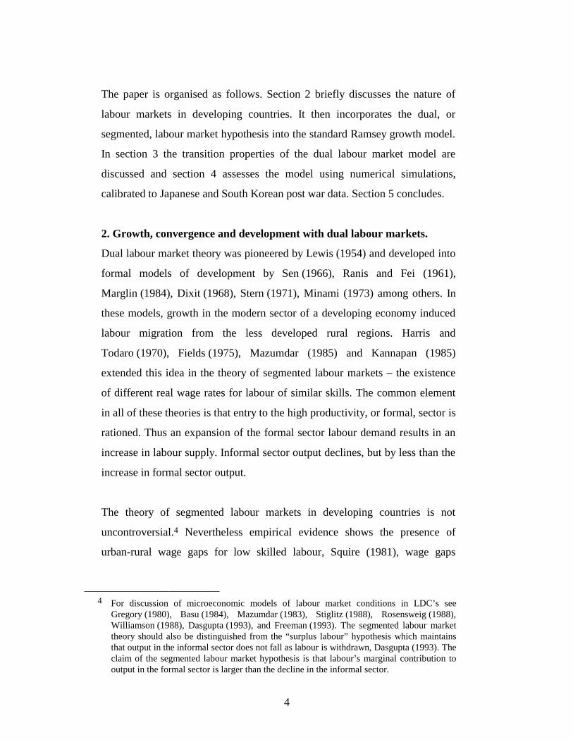
Assume u(c, l) takes the isoelastic form,

7 This result generalises in a natural way to the isoelastic case with n capital inputs. Output

will be a linearly homogenous function of all the capital inputs. For more general functionsit can be shown that the capital inputs in the reduced form production function are weightedby a number greater than 1.

8 Output is homogeneous of degree one in k, and l, where l is itself a linear function of k.Thus output is homogeneous of degree one in k. See also Dixit (1968, 1973).

8

u c l

c c

l

c c l

( , )( ) ,

ln(( ) / ),

=−

−≠

− =

−

−

1 1

1

1

1

σ σ

σ

σ

where c is a subsistence consumption level. The necessary conditions for a

maximum are;

( )c c l− − =− −σ σ λ1 0, (8a)

� ( � )λ ρλ λ= − + −f f l nk1 2 , (8b)

� ( , �)k A f k l c c nk= − − − . (8c)

A unique solution to this problem is obtained by requiring that the solution

approaches a steady state as t tends to infinity, such that consumption and

capital grow at constant rates. As t → ∞, f2(k, 1) → ∞, and so the economy

must enter phase 2. In phase 2, �l k = 0 and l = 1. Making these substitutions

the system (8a)-(8c) is identical to the standard Ramsey model. In phase 1

however, the transitional dynamics will be different from the standard model.

The next section discusses these transitional dynamic paths.

3. Transitional growth paths in a developing economy

Equation (8c) describes the evolution of the capital stock. Dividing by k, using

equation (7) and assuming that �l = �l , gives

� / ( , ) ( ) /k k g A w c c k n= − + − . (9)

Because output is a linear function of the capital stock the average product of

capital is constant and equal to g(A, w ). The formal sector of the dual labour

market economy (as described by equations 8a-8c) will experience a constant,

or rising, average product of capital in phase 1. If consumption is at the

9

subsistence level, or is constant, then the growth rate of the capital stock will

also be constant or increasing.9 Thus in phase 1 the economy behaves like the

“AK” linear endogenous growth models as discussed, for example, by King

and Rebelo (1990). This result contrasts with the standard model where

growth rates decline monotonically. In contrast to endogenous growth models,

however, the economy still approaches a long run steady state growth rate.10

Next, consider the path of consumption which is given by equations (8a) and

(8b). Combining these gives the “Keynes-Ramsey” rule for this model.

� ( )( � ) ( )

�c

c

c c

cA f f l

l

lk=−

+ − + −

σρ σ1 2 1 . (10)

In phase 1, the first term in the square brackets, A( f f l k1 2+ � ) is equal to the

average product of capital, g(A,w ) and is therefore constant or increasing. The

last term in the square brackets reflects the effect of induced changes in the

formal sector population on the rate of consumption. It is small when σ is

close to unity, and zero if σ = 1. In this case, which is empirically valid, the

growth rate of consumption will also be constant or increasing.11

The transitional dynamics are illustrated in the phase diagrams, Figures 2a and

2b. These are drawn in {c, k} space for the case where the level of technology

is constant. The equation �l (A ,w ) = 1 defines the level of k, say k , which

defines the phase 1-phase 2 boundary. Setting �k equal to zero in equation (8c),

gives an expression for the locus of stationary points for capital accumulation

9 A similar result is obtained in a descriptive growth model by Dixit (1973).10 The class of endogenous growth models based on Lucas’ (1988) model also have this

feature when no externalities are assumed. This class of models, however, have transitionaldynamics more akin to the standard Ramsey model than to models based on strictly non-convex production possibilities, as in Romer (1986).

11 The elasticity of substitution, σ, is generally thought to be around 1 or lower, Blanchard andFisher (1989).

10

per worker. Recalling that f(k, �l ) = g(A,w )k in phase 1, then �k = 0 is a ray

with slope g(A,w ) - n, which intersects the vertical axis at − c . This is shown

as line segment − c a. This intersects the curve a b d which is the �k = 0 line

in phase 2. Everywhere below − c a b d, the per worker capital stock is

increasing.

(Fig. 2a and 2b here)

Setting the growth rate of consumption per worker equal to zero in

equation (10), gives the locus of stationary points for consumption. In phase 1,

stationary consumption occurs if g(A,w ) = ρ+( )� /1− σ l l . This is independent

of the level of k when σ = 1, and the stationary consumption paths are drawn

for this case. The growth rate of consumption will be positive if g(A, w ) > ρ

and this is drawn in Figure 2a. Otherwise g(A,w ) < ρ and this is shown in

Figure 2b. In phase 2, equation (8b) defines a unique value of k, k* where

� / � /c c = =λ λ 0. This is a vertical line in Figures 2a and 2b, k*-b. To the right

of this line consumption per worker is falling and to the left it is rising.

Possible optimal trajectories are drawn from k(0) to k*.

Consider the economy as it crosses the phase 1-phase 2 boundary at k . At this

boundary it is approximately true that y = f(k , 1) ≅ g(A,w )k . But for k < k

∂ ∂y k/ = A f f lk( ( ) ( ) � )1 2⋅ + ⋅ where f l k2 ( ) �⋅ is positive. For values of k > k ,

∂ ∂y k/ = A f1( )⋅ , so that ∂ ∂y k/ falls across this boundary. From equations (9)

and (10) it follows that the growth rate of consumption and capital also fall as

the economy enters phase 2.

These results show that linear approximations of the growth rates in the

neighborhood of the steady state may be poor approximations to the growth

rate of the economy when k < k . The use of steady state conditions has been

11

widespread, in particular in the cross country econometric growth literature,

following Mankiw, et al, (1992). This result therefore indicates that if

developing economies are characterised by dual labour markets, then

regression equations based on the growth equations in the neighborhood of a

steady state may be misspecified.

Thus we have shown that the dual economy model behaves like the linear

endogenous growth model in phase 1, and that the growth pattern may change

in response to structural changes occurring during the course of development.

The next section considers these results in the light of the experience of the

Japan and South Korea.

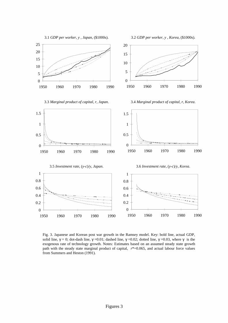
4. Numerical Solutions

King and Rebelo’s (1993) critique of the Ramsey growth model is based on

the relative magnitudes of important variables in numerical solutions. This

section therefore presents numerical solutions in order to compare the two

models further.12 First, following King and Rebelo (1993), the results of the

transitional growth paths of a Ramsey growth model are plotted against the

actual growth path of Korea and Japan in Figure 3. The solutions use a Cobb-

Douglas production function, as in Barro and Sala-i-Martin (1995) and King

and Rebelo (1993) and are parameterised using data from Summers and

Heston (1991) Penn World Table Mk. 5.6.13 For the numerical solutions the

assumption that technology is constant is relaxed so that, A t A e t( ) ( )= 0 γ . In

12 The procedure of explaining the growth of countries in an aggregate closed economy

framework is also adopted by Mankiw et al (1992), Mankiw (1995) and Barro and Sala-i-Martin (1995). The omission of the role of foreign capital may be particularly important inthis context. Nevertheless, in South Korea for example, national savings still accounted for75 percent of domestic investment during the rapid growth in the 1970’s, and up to 100percent in the 1980’s, Dornbusch and Park (1987). A full account of the Japanese and SouthKorean growth should also account for the effects of trade, technology transfer, post-warreconstruction and other government policies. The aggregate closed economy frameworkmay, nevertheless, be viewed as a useful starting point.

13 The most recent version of this data is the Penn World Table Mk 5.6 and was obtained fromthe NBER internet site http://nber.harvard.edu/pwt56.html.

12

Figure 3 results are presented for different values of γ. In all solutions,

however, the steady state marginal product of capital is held constant at 0.065,

by adjusting the discount rate, ρ, for different values of γ.

(Fig. 3 here)

The results confirm King and Rebelo’s (1993) findings. The growth rate falls

rapidly from it maximum value displaying very little persistence. This

contradicts the actual pattern of growth in Japan and South Korea. Similarly

the marginal product of capital is unrealistically high when γ is assumed to be

low. If higher values of γ are assumed the model performs better. Nevertheless

King and Rebelo’s objections are still valid as one is then explaining the

miracle by the exogenous growth rate of technology and not by endogenously

determined returns to capital.

To implement numerical solutions for the dual labour market model, we

require approximate dates at which the economies made the transition from

phase 1 to phase 2. In this context, Minami (1973, 1994) presents evidence of

“tightening” formal sector labour markets in Japan, such as reduced sectoral

and skill based wages gaps and accelerating wage increases, and concludes

that informal sector labour was exhausted around the early to mid 1960’s.

Similar evidence is presented for Korea by Bai (1982), which suggests that the

Korean labour markets tightened during the mid 1970’s.

Taking these dates as approximate timing for the phase 1 phase 2 transition

then one can determine the implied level of w .14 In addition simulations

14 Let y be the GDP in the formal sector per worker in both sectors, as above. Then in phase 1,

the share of formal sector labour in formal sector output is s w l yL ≡ . On the phase1 phase 2 boundary, l = 1, so w s yL= . Japan’s GDP per worker was $m 7.3 in 1965 andKorea’s was $m 6.2 in 1975, measured in constant 1985 dollars (PPP). Thus assuming thatthe labor share is 60 percent, gives values of w equal to $4500 for Japan and $3700 forKorea.

13

require an estimate of the size of the informal sector relative to the formal

sector. For the purpose of this exercise it is assumed that the economy-wide

GDP was initially equally divided between formal and informal activities in

the initial year.15

Figure 4 shows numerical solutions derived using these assumptions. Results

are shown for different levels of γ, with the initial level of technology, A(0),

chosen so that phase 2 is reached in 1965 for Japan and 1975 for Korea. The

numerical results confirm the analysis so far. The growth rate and marginal

product of capital are relatively persistent and increasing in some cases. In

addition investment rates are high initially and then fall in phase 2. The

relative magnitudes of prices, investment rates and growth rates are quite

plausible, and quite different to the pattern of growth in the standard Ramsey

model described by King and Rebelo (1993).

(Fig. 4 here)

Figure 5 shows the results of comparative dynamic analysis of the growth path

in response to changes in the models parameters. Cells 5.1 and 5.2 of show the

effect of different levels of w , holding constant the steady state growth

marginal product of capital, r*, the initial average product of capital

g(A(0), w ), and initial level of GDP per worker. Different exogenous wages

do not radically alter the nature of the transition, but require a higher level of y

be obtained before phase 2 is reached. Thus a higher level of w could

potentially account for Korea’s growth through to the 1990’s.

(Fig. 5 here)

15 There may also be large measurement problems. Informal sector activity is likely to be

understated in national accounts data.

14

The effects of altering the initial average product of capital (for given w , r*,

g(A(0), w )) are shown in cells 5.3 and 5.4. Higher initial levels of technology

induce a higher growth rate over phase 1 so that the growth rate increases in

response to a constant rate of technology change. This property is desirable in

that “growth miracles”, by definition, begin with an acceleration of growth

from an initially low rate.16 Cells 5.5 and 5.8 show that introducing a

minimum consumption constraint, reduces the growth rate and delays the

arrival of phase 2.

Finally cells 5.7 and 5.8 show solutions where the share of capital is varied

from 0.4 to 0.5 and 0.8, holding the initial average product of capital and w

fixed. This is of interest since Mankiw et al (1992), Barro and Sala-i-Martin

(1995) and Mankiw (1995) argue that the capital share should be about 0.6-

0.8, to take account of human capital. As the capital share increases the

production function approaches the linear case so that so there is less

difference in the growth paths between the two phases.17 The higher capital

share also results in a lower labour demand elasticity with respect to changes

in technology. Thus with a higher capital share, the marginal and average

products of capital rise more slowly as capital accumulates in phase 1.

The simulations thus indicate several desirable properties of the dual, or

segmented, labour market model in accounting for stylised facts of growth.

Specifically growth rates may be low when the capital stock is low, and a

modest rate of exogenous technology change can produce the observed pattern

of slow but accelerating growth as the average product of capital rises. This

high growth phase, however, comes to an end eventually as demand for labour

in the formal sector reaches sufficiently high levels. Further, during the high

16 Similarly large scale technology investments, such as the U.S. investment in of Japan and

Korea, may be seen has technology shifts which induce higher growth rate over phase 1.17 Also when the capital share is higher, the opportunity cost of consumption is also higher, so

that consumption tends to grow slowly and the economy has high savings and investmentrates.

15

growth phase the marginal product of capital remains relatively constant and

never exceeds 25 percent. Thus rapid growth is achieved through the

persistence of moderate marginal product of capital, rather than extremely

high but rapidly diminishing marginal product of capital.

The model is, however, highly stylised. The dualistic structure is an

oversimplification of the many segmented labour markets formal sector as is

the assumption of a constant reservation wage. A possible consequence of this

is that while the model generates a growth slowdown after the informal sector

labour supply is absorbed, Japan experienced a slowdown in growth in the

1970’s, about 10 years after Minami’s date for the tightening of labour

markets. The period of rapid growth could be extended however if w were

endogenous. The construction of multi-sector general equilibrium growth

models which endogenise the wage in the informal sector, is therefore an

interesting area for further research.18

5. Conclusion

The accelerated transition to a modern industrial economy eludes many

LDC’s. In recent literature, beginning with seminal papers by Romer (1986,

1990), Lucas (1988, 1993) and Grossman and Helpman (1992), there has been

considerable emphasis on the productivity changes such as knowledge

diffusion and positive externalities. An important insight of the standard

growth model, however, is that relatively capital scarce economies have high

average and marginal products of capital which induce rapid capital

accumulation. While the importance of this mechanism has recently been

questioned, this paper shows that a high marginal products of capital does

produce an empirically plausible growth pattern, if the economy has a dual

18 An alternative interpretation is that endogenous technology change may be relatively more

important in the latter stages of a growth miracle, for example from 1960-1970 in Japan,1980-1990 in Korea, whereas the early stages can be explained without appealing to largetechnology shifts.

16

labour market. High returns to capital are sustained by increased labour

employed in the formal sector, resulting in persistently high growth rates for

period of 15-30 years. This is in accordance with the early stages of growth in

the economies that have recently achieved successful industrialisation and

development such as South Korea and Japan.

17

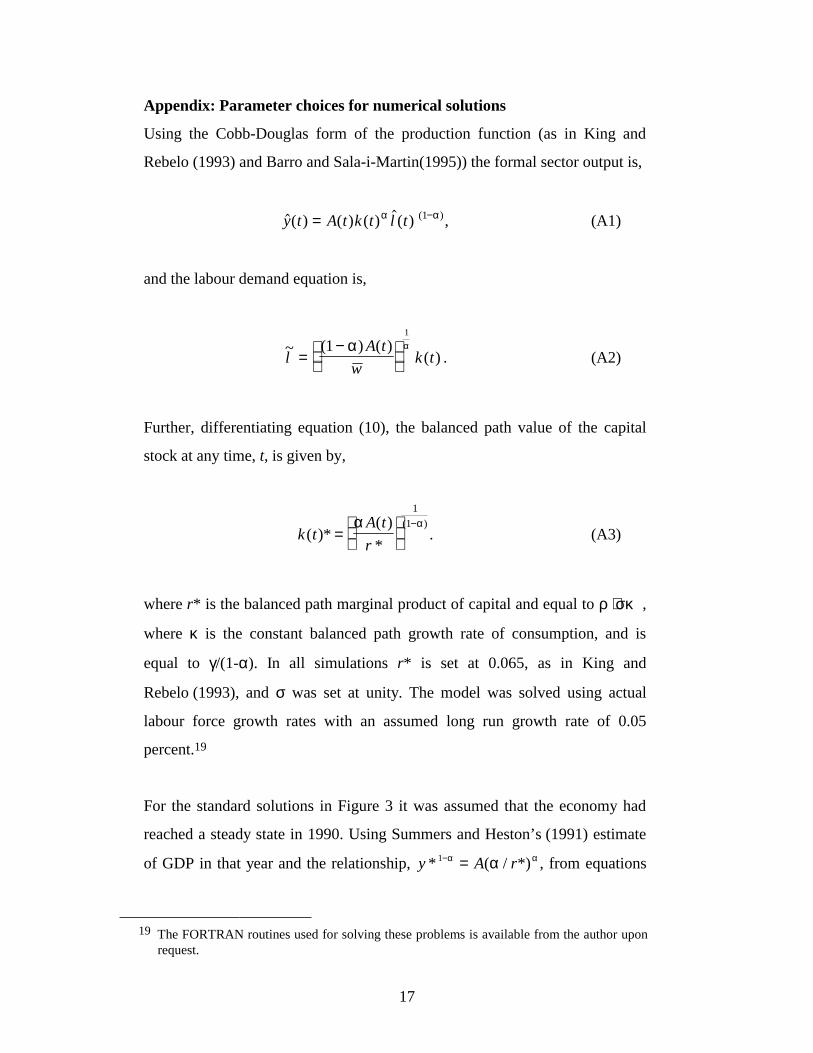
Appendix: Parameter choices for numerical solutions

Using the Cobb-Douglas form of the production function (as in King and

Rebelo (1993) and Barro and Sala-i-Martin(1995)) the formal sector output is,

�( ) ( ) ( ) �( ) ( )y t A t k t l t= −α α1 , (A1)

and the labour demand equation is,

~ ( ) ( )( )l

A t

wk t=

−

11

α α. (A2)

Further, differentiating equation (10), the balanced path value of the capital

stock at any time, t, is given by,

k tA t

r( )*

( )

*

( )=

−α α1

1. (A3)

where r* is the balanced path marginal product of capital and equal to ρ + σκ,

where κ is the constant balanced path growth rate of consumption, and is

equal to γ/(1-α). In all simulations r* is set at 0.065, as in King and

Rebelo (1993), and σ was set at unity. The model was solved using actual

labour force growth rates with an assumed long run growth rate of 0.05

percent.19

For the standard solutions in Figure 3 it was assumed that the economy had

reached a steady state in 1990. Using Summers and Heston’s (1991) estimate

of GDP in that year and the relationship, y A r* ( / *)1− =α αα , from equations

19 The FORTRAN routines used for solving these problems is available from the author upon

request.

18

(A1) and (A3), determines the value of A(t), for t = 1990. The remaining

values can be calculated as A(t) =A e t( ) ( )1990 1990− −γ . Given A(0), k(0), and k*,

the differential equation system (8b) and (8c) was integrated using finite

difference method for the solution a the two point boundary value problem –

the “relaxation method”, as described in Press et al (1990).

For the numerical solutions of dual labour market model require values of w ,

as described above, and the initial marginal product of capital, given by

( / )y k α = A w(( ) / )1 1− −α α . Given, y, then this expression determines A.

Identical numerical procedures were used to solve the model in this case and

the parameters of the production function and utility function were as for the

standard model, with the same long run steady state growth path.

References

Amsden, A.H., Asia’s New Giant: South Korea and Late Industrialisation,Oxford University Press, N.Y., 1989.

Bai, Moo Ki., “The Turning Point in the Korean Economy”, The DevelopingEconomies, 20, pp. 117-140, 1982.

Barro Robert J. and Xavier Sala-i-Martin, Economic growth, McGraw Hill,Singapore, 1995.

Barro, Robert J. and Xavier Sala-i-Martin, “Convergence”, Journal ofPolitical Economy, 100, 2, pp. 223-351, 1992.

Basch, Michael and Ricardo D. Paredes–Molina, “Are there Dual LabourMarkets in Chile?: Empirical evidence”, Journal of DevelopmentEconomics, 50, pp. 297-312, 1996.

Basu, Kaushik, The Less Developed Economy: A Critique of ContemporaryTheory, B. Blackwell, Oxford, 1984.

Becker, C. M., A.H. Hamer and A. R. Morrison, Beyond Urban Bias inAfrica: Urbanisation in an Era of Structural Adjustment, HeinemannPortsmouth, NH., 1994.

Blanchard, Oliver Jean and Stanley Fisher, Lectures on Macroeconomics,The MIT Press, 1989.

Bliss, Christopher and Nicholas Stern, “Productivity, Wages and Nutrition:Part II: Some Observations”, Journal of Development Economics,5,4, pp. 363-398, 1978.

19

Caselli, F., G. Esquivel and F. Lefort, “Reopening the Convergence Debate:A New Look at Cross-Country Growth Empirics”, Journal ofEconomic Growth, 1,4, pp. 363-389, 1996.

Dasgupta, Partha, An inquiry into well-being and destitution, OxfordUniversity Press, Oxford, 1993.

Dixit, A.K., “Growth Patterns in a Dual Economy”, Oxford EconomicPapers, 22, 2, pp. 229-234, 1971.

Dixit, A.K., “Optimal Development in a Labour Surplus Economy”, Reviewof Economic Studies, 35, pp. 171-184, 1968.

Dixit, A.K., “Models of Dual Economies”, in: J.A. Mirrlees and N. H. Stern(eds), Models of Economic Growth, John Wiley and Sons, pp. 325-357, 1973.

Dornbusch, R. and Yung Chul Park, Korean Growth Policy, BrookingsPapers on Economic Activity, 0, 2, pp. 389-444, 1987.

Fei, John C., K. Ohkawa and Gustav Ranis, “Economic Development inHistorical Perspective: Japan, Korea and Taiwan”, in Japan and theDeveloping countries, K. Ohkawa and G. Ranis (eds), BasilBlackwell, N.Y., 1985.

Fields, Gary S., “Rural-urban migration, urban unemployment andunderemployment, and Job Search activity in LDC’s”, Journal ofDevelopment Economics, 2, 2, pp. 165-187, 1975.

Fields, Gary S. and Henry Wan Jr., “Wage setting institutions and EconomicGrowth”, World Development, 17, 9, pp. 1471-1483, 1989.

Fields, Gary S., “Changing Labour Market Conditions and EconomicDevelopment in Hong Kong, the Republic of Korea, Singapore, andTaiwan, China”, The World Bank Economic Review, 8, 3, pp. 395-414, 1994.

Freeman, R.B., “Labour markets in low income countries”, in H. Chenery andT.N. Srinivasan (ed’s), Handbook of Development Economics, NorthHolland, 1988.

Freeman, R.B., “Labour Markets and Institutions in EconomicDevelopment”, American Economic Review, 83,2, pp. 403-408, 1993.

Gregory, Peter, An Assessment of Changes in Employment conditions inLess Developed Countries”, Economic Development and CulturalChange, 28,4, pp. 673-700, 1980.

Grossman, Gene M. and Elhanan Helpman, Innovation and Growth in theGlobal Economy, MIT Press, Cambridge, Massachusetts, 1992.

Ghatak, Subrata., Paul Levine and Stephen Wheatley-Price, MigrationTheories and Evidence: An Assessment, Journal of EconomicSurveys, 10, 2, pp. 159-198, 1996

20

Harris, J. R. and M.P. Todaro, “Migration, Unemployment and Development:A Two Sector Analysis”, American Economic Review, 60,3, pp. 126-42, 1970.

Havrylyshyn, O., “Trade policy and productivity gains in developingcountries: A survey of the literature”, The World Bank ResearchObserver, 5,1, pp. 1-24, 1990.

Kannappan, Subbiah, “Urban Employment and the Developing Nations”,Economic Development and Cultural Change, 33, pp. 669-730, 1985.

Kim, Jong-Il and Lawrence Lau, “The Role Of Human Capital in theEconomic Growth of the East Asian Newly IndustrialisingCountries”, Manuscript, Department of Economics, StanfordUniversity, 1993.

King, R.G. and S. T. Rebelo, “Transitional Dynamics and Economic Growthin the Neoclassical Model”, American Economic Review, 83,4, pp.908-929, 1993.

King, R.G. and S. T. Rebelo, “Public Policy and Economic Growth:Developing Neoclassical Implications”, Journal of PoliticalEconomy, 98,5, pt.2, pp. S126-S150, 1990.

Leibenstein, Harvey, “The Theory of Underdevelopment in DenselyPopulated Backward Areas,” in, Efficiency Wage Models of theLabour Market, G. Akerlof and J. Yellen (eds), CambridgeUniversity Press, New York, 1986.

Lewis, W.A., “Economic Development with Unlimited Supplies of Labour”,Manchester School, 22,2, pp. 139-191, 1954.

Lucas, Robert E., “On the Mechanics of Economic Development”, Journal ofMonetary Economics, 22,1, pp. 3-42, 1988.

Lucas, Robert E., “Making a Miracle” Econometrica, 61,2, pp. 251-272, 1993.

Magnac, Th., “Segmented or Competitive Labour Markets?”, Econometrica,59, 1, pp. 165-188, 1991.

Mankiw, N.G., “The Growth of Nations”, Brookings papers on economicactivity, 1, pp. 275-326, 1995.

Mankiw, N.G., D. Romer and D. N. Weil, “A Contribution to the Empirics ofEconomic Growth”, The Quarterly Journal of Economics, 107,2, pp.407-437, 1992.

Marcouiller, D., V. Ruiz de Castilla and Woodruff, “Formal Measures of theInformal Sector Wage Gap in Mexico, El Salvador and Peru”, BostonCollege Working Papers in Economics, March 28, 1995.

Marglin, Stephen A., Growth, Distribution, and Prices, Cambridge, Mass,Harvard University Press, 1984.

Mazumdar, D., “Segmented Labour Markets in LDC’s”, American EconomicReview, 73, 3, pp. 254-259, 1983.

21

Mazumdar, D., “Paradigms in the Study of Urban Labour Markets in LDC’s:A Reassessment in the Light of an Empirical Summary in BombayCity”, World Bank Staff Working Paper, No 366, December 1979.

Minami Ryoshin, The Turning Point in Economic Development, Japan'sExperience, Economic Research series, No. 14, The Institute ofEconomic Research, Hitotsubashi University, 1973.

Minami Ryoshin, The Economic Development of Japan, A Quantitative Study,2nd edition, St Martins Press, N.Y., 1994.

Ohkawa, Kaushi and Henry Rosovsky, Japanese Economic Growth, TrendAcceleration in the Twentieth Century, Stanford University Press,1973.

Olson, Jr., Mancur, “Big Bills Left on the Sidewalk: Why Some Nations areRich and Others Poor”, Journal of Economic Perspectives, 10, 2,pp. 3-24, 1996.

Pilat Dirk, The Economics of Rapid Growth, The Experience of Japan andKorea, Edward Elgar, Vermont, 1994

Press W.H., B.P. Flannery, S.A. Teukolsky, and W.T. Vetterling, NumericalRecipes: The Art of Scientific Computing, Cambridge UniversityPress, 1990.

Ranis, Gustav, and J.C.H. Fei, “A Theory of Economic Development”,American Economic Review, September, 51, 4, pp. 533-65, 1961.

Ranis, Gustav, “Another Look at the East Asian Miracle”, The World BankEconomic Review, 9, 3, pp. 509-534, 1995.

Romer, Paul M., “Increasing Returns and Long Run Growth”, Journal ofPolitical Economy, October 1986, 94,5, pp. 1002-37.

Romer, Paul. M., “Endogenous Technological Change”, Journal of PoliticalEconomy, 98, 5, pt.2, pp. S71-S102, 1990.

Rosenzweig, M.R., “Labour Markets in Low Income Countries”, in H.Chenery and T.N. Srinivasan (ed’s), Handbook of DevelopmentEconomics, North Holland, 1988.

Sala-i-Martin, Xavier, “Cross Section Regressions and the Empirics ofEconomic Growth”, European Economic Review, 38, pp. 731-738,1994

Sen, A.K., “Peasants and Dualism With or Without Surplus Labour”, Journalof Political Economy, 74: pp. 425-450, 1966.

Solow, R. M., “A Contribution to Theory of Economic Growth”, TheQuarterly Journal of Economics, 70, 1, pp. 65-94, 1956.

Squire, Lyn., Economic Policy in Developing Countries: A Survey of Issuesand Evidence, Oxford University Press, Oxford, 1981.

Stern, N, H., “Optimal Development in a Dual Economy”, Review ofEconomic Studies, 39,2, pp. 171-84, 1972.

22

Stiglitz, J.E., “Economic Organisation, in H. Chenery and T.N. Srinivasan(ed’s), Handbook of Development Economics, North Holland, 1988.

Summers, Robert and Alan Heston, “The Penn World Table (mark 5); anexpanded set of international comparisons, 1950-1988, QuarterlyJournal of Economics 106, May, 1991.

Sundrum, R. M., Income distribution in less developed countries, Routledge,London, 1990.

Swan, T. W., “Economic Growth and Capital Accumulation” EconomicRecord, November, 32, pp. 334-361, 1956.

Williamson, J.G., “Migration and Unemployment”, in H. Chenery and T.N.Srinivasan (ed’s), Handbook of Development Economics, NorthHolland, 1988.

Williamson J. G., “Human Capital Deepening, Inequality and DemographicEvents along the Asia-Pacific Rim”, in Naohiro Ogawa, Gavin Jonesand J. G. Williamson (eds), Human Resouces in Development alongthe Asia-Pacific Rim, Singapore, Oxford University Press, 1993

World Bank, The East Asian Miracle: Economic Growth and Public Policy,Oxford University Press, New York, N.Y, 1993

Young, Alwyn, “The Tyranny of Numbers: Confronting the StatisticalRealities of the East Asian Growth Experience”, Quarterly Journal ofEconomics, 110, 3, pp. 641-680, 1995.

Young, Alwyn, Lessons from the East Asian NICs: A contrarian view",European Economic Review, 38, pp. 964-973, 1994.

Figures 1

6

7

8

9

10

11

1950 1960 1970 1980 1990

Japan

South East Asia

North East Asia

SouthKorea

6

7

8

9

10

11

1950 1960 1970 1980 1990

Latin America

South Asia

Africa

USA

Fig. 1. Post war economic growth in the developing regions, natural logarithim of GDP perworker, $1995 PPP. Source: Summers and Heston, (1991), Penn World Table, Mk 5.6.Region definitions: “North East Asia” is Taiwan, Hong Kong and China; “South Asia” isBangladesh, India, Pakistan and Sri-Lanka; “South East Asia” is Indonesia, Malaysia,Singapore, Philippines and Thailand. “Latin America” consists of countries 52, 55, 57,58, 60-67, 71, 73-84 in the Summers and Heston (1991) country code. “Africa” consists of countries1-50 in the Summers and Heston (1991) country code, excluding 13, Djibouti, and 41, SouthAfrica.

Figures 2

k k*

a

b

c

k

d

k( )0

c( )0

− c

�c = 0

�k = 0

Figure 2a: Phase Diagram when g(A,w ) > ρ.Note: Diagram drawn for σ = 1 and g = 0.

k k*

a

b

c

k

d

k( )0

c( )0

− c

�k = 0

�c = 0

Fig. 2b: Phase Diagram when g(A,w ) < ρ.Note: Diagram drawn for σ = 1 and g = 0.

Figures 3

3.1 GDP per worker, y , Japan, ($1000s). 3.2 GDP per worker, y , Korea, ($1000s).

0

5

10

15

20

25

1950 1960 1970 1980 1990

0

5

10

15

20

1950 1960 1970 1980 1990

3.3 Marginal product of capital, r, Japan. 3.4 Marginal product of capital, r, Korea.

0

0.5

1

1.5

1950 1960 1970 1980 1990

0

0.5

1

1.5

1950 1960 1970 1980 1990

3.5 Investment rate, (y-c)/y, Japan. 3.6 Investment rate, (y-c)/y, Korea.

0

0.2

0.4

0.6

0.8

1

1950 1960 1970 1980 1990

0

0.2

0.4

0.6

0.8

1

1950 1960 1970 1980 1990

Fig. 3. Japanese and Korean post war growth in the Ramsey model. Key: bold line, actual GDP,solid line, γ = 0; dot-dash line, γ =0.01; dashed line, γ =0.02; dotted line, γ =0.03, where γ is theexogenous rate of technology growth. Notes: Estimates based on an assumed steady state growthpath with the steady state marginal product of capital, r*=0.065, and actual labour force valuesfrom Summers and Heston (1991).

Figures 4

4.1 GDP per worker, y , Japan, ($1000s) 4.2 GDP per worker, y , Korea, ($1000s)

0

10

20

30

1950 1960 1970 1980 1990

0

5

10

15

1950 1960 1970 1980 1990

4.3 Marginal product of capital, r, Japan. 4.4 Marginal product of capital, r, Korea.

0

0.1

0.2

0.3

1950 1960 1970 1980 1990

0

0.1

0.2

0.3

1950 1960 1970 1980 1990

4.5 Investment rate, (y-c)/y, Japan. 4.6 Investment rate, (y-c)/y, Korea.

0

0.2

0.4

0.6

0.8

1950 1960 1970 1980 1990

0

0.2

0.4

0.6

0.8

1950 1960 1970 1980 1990

Fig. 4. Japanese and Korean post war growth in the dual, or segmented, labour market model. Key:bold line, actual GDP, solid line, γ = 0; dot-dash line, γ =0.01; dashed line, γ =0.02; dotted line, γ =0.03, where γ is the exogenous rate of technology growth. Notes: Estimates based on an assumedsteady state growth path with the steady state marginal product of capital, r*=0.065, and actuallabour force values from Summers and Heston (1991).

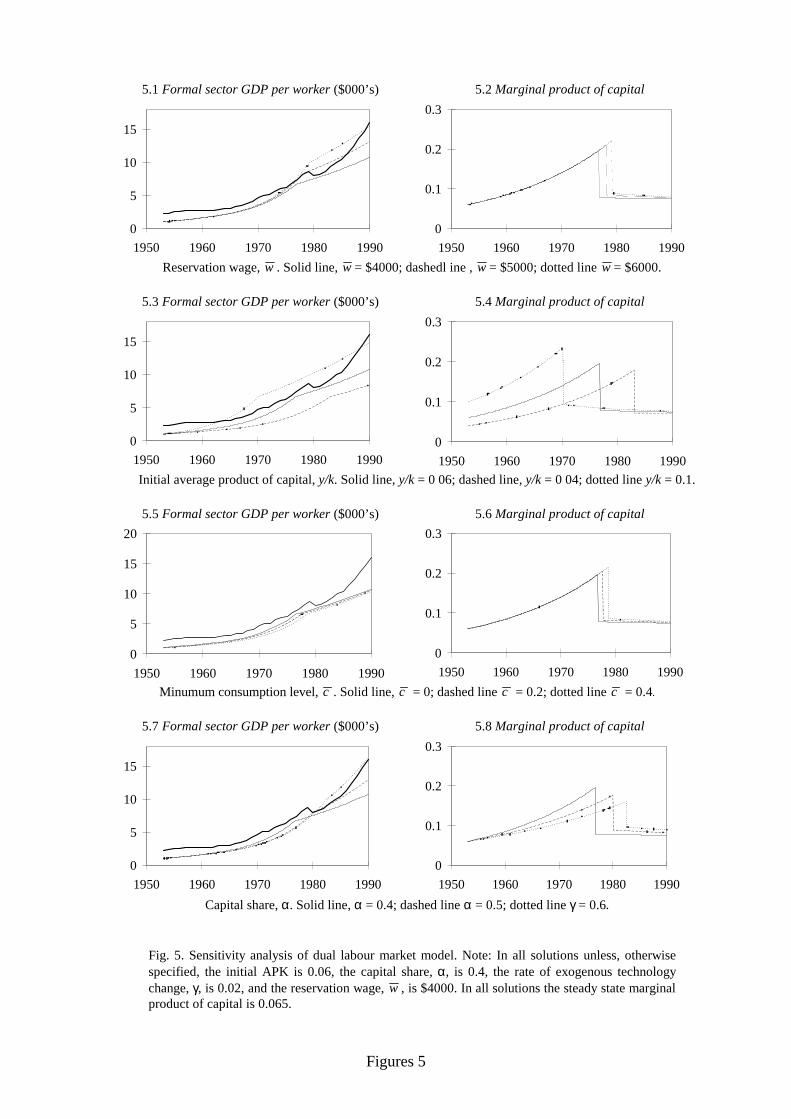
Figures 5

5.1 Formal sector GDP per worker ($000’s) 5.2 Marginal product of capital

0

5

10

15

1950 1960 1970 1980 1990

0

0.1

0.2

0.3

1950 1960 1970 1980 1990

Reservation wage, w . Solid line, w = $4000; dashedl ine , w = $5000; dotted line w = $6000.


0

5

10

15

1950 1960 1970 1980 19900

0.1

0.2

0.3

1950 1960 1970 1980 1990

Initial average product of capital, y/k. Solid line, y/k = 0 06; dashed line, y/k = 0 04; dotted line y/k = 0.1.


0

5

10

15

20

1950 1960 1970 1980 1990

0

0.1

0.2

0.3

1950 1960 1970 1980 1990

Minumum consumption level, c . Solid line, c = 0; dashed line c = 0.2; dotted line c = 0.4.


0

5

10

15

1950 1960 1970 1980 1990

0

0.1

0.2

0.3

1950 1960 1970 1980 1990

Capital share, α. Solid line, α = 0.4; dashed line α = 0.5; dotted line γ = 0.6.

Fig. 5. Sensitivity analysis of dual labour market model. Note: In all solutions unless, otherwisespecified, the initial APK is 0.06, the capital share, α, is 0.4, the rate of exogenous technologychange, γ, is 0.02, and the reservation wage, w , is $4000. In all solutions the steady state marginalproduct of capital is 0.065.

transitional growth paths in developing economies...transitional growth paths in developing...

Documents