Translating Soils Information

for Hydrological Modelling Reflecting on the Big Picture from the 1970s

to the Present

Roland Schulze Professor Emeritus of Hydrology & Senior Research Associate

Centre for Water Resources Research School of Agricultural, Earth & Environmental Sciences

University of KwaZulu-Natal, Pietermaritzburg, RSA

Defining Moments …From Way Back !

1. “A vital role is played by soil, for it is the capacity of the soil to absorb, retain and release water that is the prime regulator of the evapotranspiration and runoff response of a catchment” (England & Stephenson, 1970)

2. A catchment is not a lumped system in regard to soils, and pronounced differences in magnitude and sequence of hydrological processes have been observed in soil units within a catchment (England, 1970)

3. “Soils of the Tugela Basin” (van der Eyk et al., 1969)

Falling in Love …With a Subject MatterDefining Years …1970 -1974

The Drakensberg

Cathedral Peak Research Catchments

Energy and Water Budgets on Slopes with Different Gradients & Aspects

‘TOP’ OF THE ATMOSPHERE

EXTRATERRESTRIAL RADIATION

Solar Constant (1361 W.m-2)

Earth’s Radius Vector (Time of Year)

Angle of Inclination

(Latitude; Time of Year; Time of Day)

Direct Radiation ATTENUATIONS

Atmosphere (Water Vapour; Aerosols; Altitude; Optical Air mass)

Terrain (Slope; Aspect; Albedo)

Cloud (Type; Time of Day)

N

E

S

W ASPE

DALT Normal to Slope N

S

AZIM

ALT

W

N

S

E

SLP

THET

Diffuse Radiation ATTENUATIONS

Solar Altitude

Slope

(b) HORIZON SHADING ALT < HOR

(a) SLOPE SHADING ALT < SLP

ALT

HOR

ALT

SLP

1000 -

750 -

500 -

250 -

0 - 17 16 15 14 13 12 11 10 9 8 7

Time of Day (h)

Glo

bal

Rad

iati

on

Flu

xes

(W.m

-2)

- - - 35o NNW (290o)

32o S (170o)

NOVEMBER 20, 1986

Mapping Energy

Budgets on Sloping Terrain

Considerations

Verification

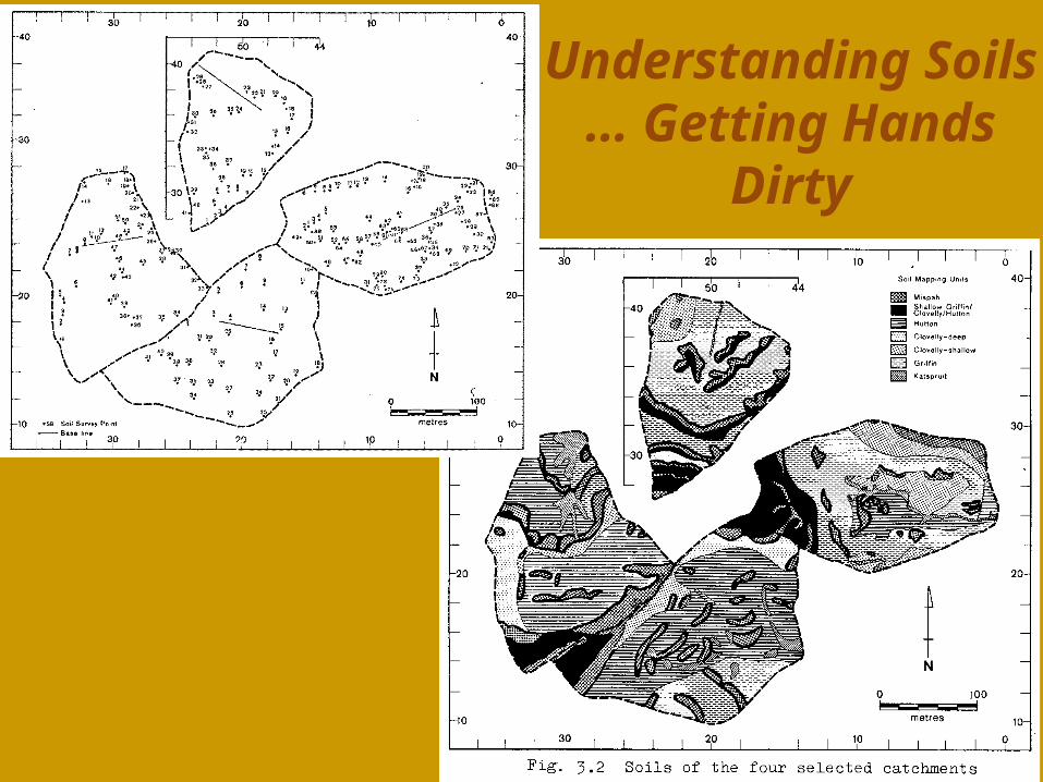
Understanding Soils … Getting Hands

Dirty

Land Cover Class Land Treatment/Practice/Description

Stormflow Potential

Hydrological Soil Group A A/B B B/C C C/D D

Veld (range) and Pasture

1 = Veld/pasture in poor condition 2 = Veld/pasture in fair condition 3 = Veld/pasture in good condition 4 = Pasture planted on contour 5 = Pasture planted on contour 6 = Pasture planted on contour

High Moderate Low High Moderate Low

68 49 39 47 25 6

74 61 51 57 46 14

79 69 61 67 59 35

83 75 68 75 67 59

86 79 74 81 75 70

88 82 78 85 80 75

89 84 80 88 83 79

Irrigated Pasture Low 35 41 48 57 65 68 70 Meadow Low 30 45 58 65 71 75 81 Woods and Scrub

1 = Woods 2 = Woods 3 = Woods 4 = Brush - Winter rainfall region

45 36 25 28

56 49 47 36

66 60 55 44

72 68 64 53

77 73 70 60

77 73 70 60

83 79 77 66

Orchards 1 = Winter rainfall region, understory of crop cover 39 44 53 61 66 69 71

Forests & Plantations

1 = Humus depth 25mm; Compactness: 2 = " " " 3 = " " " 4 = Humus depth 50mm; Compactness: 5 = " " " 6 = " " " 7 = Humus depth 100mm; Compactness: 8 = " " " 9 = " " " 10 = Humus depth 150mm; Compactness: 11 = " " " 12 = " "

compact moderate friable compact moderate friable compact moderate friable compact moderate friable

52 48 37 48 42 32 41 34 23 37 30 18

62 58 49 58 54 45 53 47 37 49 43 33

72 68 60 68 65 57 64 59 50 60 56 47

77 73 66 73 70 62 69 64 56 66 61 52

82 78 71 78 75 67 74 69 61 71 66 57

85 82 74 82 78 71 77 72 64 74 69 61

87 85 77 85 81 74 80 75 67 77 72 65

Urban / Sub-Urban Land Uses

1 = Open spaces, parks, cemeteries 75% grass cover 2 = Open spaces, parks, cemeteries 75% grass cover 3 = Commercial/business areas 85% grass cover 4 = Industrial districts 72% impervious 5 = Residential: lot size 500m2 65% impervious 6 = " " 1000m2 38% impervious 7 = " " 1350m2 30% impervious 8 = " " 2000m2 25% impervious 9 = " " 4000m2 20% impervious 10 = Paved parking lots, roofs, etc. 11 = Streets/roads: tarred, with storm sewers, curbs 12 = " gravel 13 = " dirt 14 = " dirt-hard surface

39 49 89 81 77 61 57 54 51 98 98 76 72 74

51 61 91 85 81 69 65 63 61 98 98 81 77 79

61 69 92 88 85 75 72 70 68 98 98 85 82 84

68 75 93 90 88 80 77 76 75 98 98 88 85 88

74 79 94 91 90 83 81 80 78 98 98 89 87 90

78 82 95 92 91 85 84 83 82 98 98 90 88 91

80 84 95 93 92 87 86 85 84 98 98 91 89 92

1979 SCS Manual Effects of SCS Soil Groups on Curve Numbers

0

2

4

6

8

10

0

10

20

A/B B/C D

Pe

ak

Dis

cha

rge

(m

3 /s)

Sto

rmfl

ow

(m

m)

SCS Soil Group

Sensitivity of Hydrological Responsesto SCS Soil Groups

How Sensitive are Stormflow Volume & Peak Discharge to SCS Soil Groups?

Example

Catchment Area = 2 km² Precipitation = 50 mm Land Cover = Veld in fair condition Catchment Slope = 8 % Length of main Stream = 1 500 m

Conclusion Highly sensitive

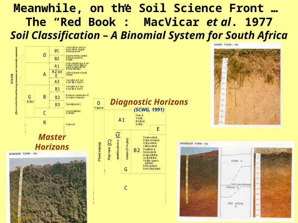
Meanwhile, on the Soil Science Front … The “Red Book”: MacVicar et al. 1977

Soil Classification – A Binomial System for South Africa01

02

A1A2 or

E

A3

B1

B2

B3

O

A

B

C

R

G(Gley)

Loose leaves and or-ganic debris, largelyundecomposed

Organic debris, partial-ly decomposed ormatted

Dark coloured due to ad-mixture of humified or-ganic matter with themineral fraction

Maximum expression ofB horizon character

Transitional to C

Unconsolidatedmaterial

Hard rock

Light coloured mineralhorizon

Transition to B butmore like A than B

Transition to A butmore like B than A

Master Horizons

(MacVicar et al., 1977)

O

A1

E

B2

G

C

Organic

HumicVerticMelanicOrthic

PedocutanicPrismacutanicGleycutanicLithocutanic

NeocutanicFerrihumic

Hard plinthicSoft plinthicYellow-brown

apedalRed apedalRed structured

Diagnostic Horizons (SCWG, 1991)

QUICKFLOW

RUNOFF

INTERCEPTION

PRECIPITATION

GROUNDWATER STORE

INTERMEDIATE STORE

SUBSOIL

TOPSOIL

SURFACE LAYER

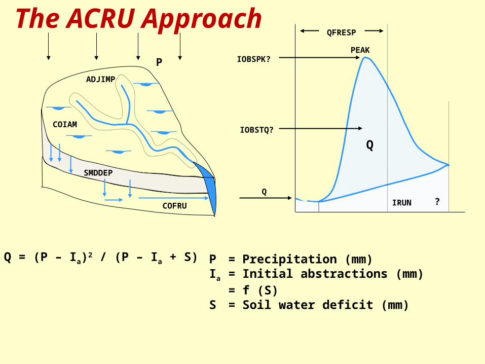
Early 1980s The beginnings of ACRU A physical-conceptual, process based,

daily time step water budget model

?

QIOBSTQ?

IOBSPK?PEAK

QFRESP

IRUNQ

P

ADJIMP

COIAM

SMDDEP

COFRU

P = Precipitation (mm)Ia = Initial abstractions (mm)

= f (S)S = Soil water deficit (mm)

Q = (P – Ia)2 / (P – Ia + S)

The ACRU Approach

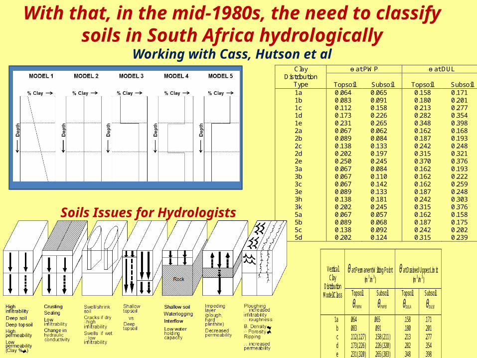
With that, in the mid-1980s, the need to classify soils in South Africa hydrologically

Working with Cass, Hutson et al

Clay Distribution

Type

ɵ at PWP ɵ at DUL

Topsoil

Subsoil

Topsoil

Subsoil 1a 1b 1c 1d 1e 2a 2b 2c 2d 2e 3a 3b 3c 3e 3h 3k 5a 5b 5c 5d

0.064 0.083 0.112 0.173 0.231 0.067 0.089 0.138 0.202 0.250 0.067 0.067 0.067 0.089 0.138 0.202 0.067 0.089 0.138 0.202

0.065 0.091 0.158 0.226 0.265 0.062 0.084 0.133 0.197 0.245 0.084 0.110 0.142 0.133 0.181 0.245 0.057 0.068 0.092 0.124

0.158 0.180 0.213 0.282 0.348 0.162 0.187 0.242 0.315 0.370 0.162 0.162 0.162 0.187 0.242 0.315 0.162 0.187 0.242 0.315

0.171 0.201 0.277 0.354 0.398 0.168 0.193 0.248 0.321 0.376 0.193 0.222 0.259 0.248 0.303 0.376 0.158 0.175 0.202 0.239

Vertical Clay

Distribution Model/Class

θ at Permanent Wilting Point (m3/m3)

θ at Drained Upper Limit (m3/m3)

Topsoil

θPWPA Subsoil

θPWPB Topsoil

θDULA Subsoil

θDULB 1a b c d e 2a b c d e 3a b c e h k 5a b c d

.064 .083 .112(.127) .173(.226) .231(.320) .067 .089 .138(.169) .202(.273) .250(.352) .067 .067(.054) .067(.054) .089(.091) .138(.169) .202(.273) .067 .089 .138 .202

.065 .091 .158(.211) .226(.320) .265(.383) .062 .084 .133(.169) .197(.273) .245(.352) .084 .110(.132) .142(.185) .133(.169) .181(.247) .245(.352) .057 .068 .092 .124

.158 .180 .213 .282 .348 .162 .187 .242 .315 .370 .162 .162 .162 .187 .242 .315 .162 .187 .242 .315

.171 .201 .277 .354 .398 .168 .193 .248 .321 .376 .193 .222 .259 .248 .303 .376 .156 .175 .202 .239

Soils Issues for Hydrologists

And, the Advent of Soils LAND TYPES from the Binomial Soil Classification, and their Databases

# Based on relatively uniform climate, terrain, soil patterns # With detailed soils inventory on soil series, clay %, texture class, profile thickness… # With the Land Type made up of several soil series# Including information on Terrain Units making up a Land Type

“Translating” Land Type Information to Hydrological Model Needs

Rules for Partitioning Soil Horizon Thicknesses

Drilling Down to Terrain Unit Level

BASIC PREMISE

Operational hydrological models should be able to be “driven” by standard datasets which are freely available from national networks and by standard (usually non-hydrological) spatial digital information available at national level, suitably “translated” (I.e. converted) into model input variables, for the models then to operate over a range of desired spatial scales

Result … Detailed mapping of soil attributes which are critical to hydrological modelling from 16600+ Land Type Polygons

(Schulze and Horan, 2008)

Result … Detailed mapping of soil attributes which are critical to hydrological

modelling (Schulze and Horan, 2008)

Result … Detailed mapping of soil attributes which are critical to hydrological modelling (Schulze and Horan, 2008; Schulze,

2012)

Quo vadis? An operational hydrologist’s perspective

Operationalising terrain unit delineation Mapping soil fertility in detail Getting a better handle on hydraulic conductivity Towards a general model of interflow Ringfencing soils with high organic matter content More detailed delineation of wetlands soils Delineating unstable soils for hydrological

modelling Getting a better handle on drainage rates of soils