Transmission Lines

The problem of plane waves propagating in air represents an example

of unguided wave propagation. Transmission lines and waveguides offer

an alternative way of transmitting signals in the form of guided wave

propagation. Transmission lines are typically electrically large (several

wavelengths) such that we cannot accurately describe the voltages and

currents along the transmission line using a simple lumped-element

equivalent circuit. We must use a distributed-element equivalent circuit

which describes each short segment of the transmission line by a lumped-

element equivalent circuit.

Consider a simple uniform two-wire transmission line with its

conductors parallel to the z-axis as shown below.

Uniform transmission line - conductors and insulating medium

maintain the same cross-sectional geometry along the entire

transmission line.

The equivalent circuit of a short segment Äz of the two-wire transmission

line may be represented by simple lumped-element equivalent circuit.

R = series resistance per unit length (Ù/m) of the transmission line

conductors.

L = series inductance per unit length (H/m) of the transmission line

conductors (internal plus external inductance).

G = shunt conductance per unit length (S/m) of the media between

the transmission line conductors.

C = shunt capacitance per unit length (F/m) of the transmission line

conductors.

We may relate the values of voltage and current at z and z+Äz by

writing KVL and KCL equations for the equivalent circuit.

KVL

KCL

Grouping the voltage and current terms and dividing by Äz gives

Taking the limit as Äz 6 0, the terms on the right hand side of the equations

above become partial derivatives with respect to z which gives

Time-domain

transmission line

equations

(coupled PDE’s)

For time-harmonic signals, the instantaneous voltage and current may be

defined in terms of phasors such that

The derivatives of the voltage and current with respect to time yield jù

times the respective phasor which gives

F re q u e n c y -d o m a in

(phasor) transmission

line equations

(coupled DE’s)

Note the similarity in the functional form of the time- and frequency-

domain transmission line equations to the respective source-free Maxwell’s

equations (curl equations). Even though these equations were derived

without any consideration of the electromagnetic fields associated with the

transmission line, remember that circuit theory is based on Maxwell’s

equations.

Given the similarity of the phasor transmission line equations to

Maxwell’s equations, we find that the voltage and current on a transmission

line satisfy wave equations. These voltage and current wave equations are

derived using the same techniques as the electric and magnetic field wave

equations. Beginning with the phasor transmission line equations, we take

derivatives of both sides with respect to z.

We then insert the first derivatives of the voltage and current found in the

original phasor transmission line equations.

The voltage and current wave equations may be written as

where ã is the complex propagation constant of the wave on the

transmission line given by

Just as with unguided waves, the real part of the propagation constant (á)

is the attenuation constant while the imaginary part (â) is the phase

constant. The general equations for á and â in terms of the per-unit-length

transmission line parameters are

The general solutions to the voltage and current wave equations are

~~~~~ ~~~~~

+z-directed waves !z-directed waves _ a

The current equation may be written in terms of the voltage coefficients

through the original phasor transmission line equations.

oThe complex constant Z is defined as the transmission line characteristic

impedance and is given by

The transmission line equations written in terms of voltage coefficients

only are

The complex voltage coefficients may be written in terms of magnitude and

phase as

The instantaneous voltage becomes

The wavelength and phase velocity of the waves on the transmission line

may be found using the points of constant phase as was done for plane

waves.

Lossless Transmission Line

If the transmission line loss is neglected (R = G = 0), the equivalent

circuit reduces to

Note that for a true lossless transmission line, the insulating medium

between the conductors is characterized by a zero conductivity (ó = 0), and

real-valued permittivity å and permeability ì (åO = ìO= 0). The

propagation constant on the lossless transmission line is

Given the purely imaginary propagation constant, the transmission line

equations for the lossless line are

The characteristic impedance of the lossless transmission line is purely real

and given by

The phase velocity and wavelength on the lossless line are

Example (Lossless coaxial transmission line)

The dominant mode on a coaxial transmission line is the TEM

z z(transverse electromagnetic) mode defined by E = H = 0. Due to the

symmetry of the coaxial transmission line, the

transverse fields are independent of ö. Thus,

we may write

Between the conductors, the fields must

satisfy the source-free Maxwell’s equations:

ñ öThe field components E and H are related to the transmission line voltage

and current by

1If we integrate the Faraday’s law equation along the path C and integrate

2the Ampere’s law equation along the path C ,

which are the lossless transmission line equations.

Terminated Lossless Transmission Line

If we choose our reference point (z = 0) at the load termination, then

the lossless transmission line equations evaluated at z = 0 give the load

voltage and current.

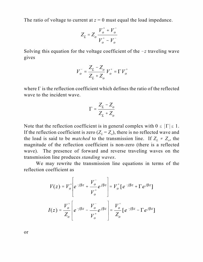
The ratio of voltage to current at z = 0 must equal the load impedance.

Solving this equation for the voltage coefficient of the !z traveling wave

gives

where à is the reflection coefficient which defines the ratio of the reflected

wave to the incident wave.

Note that the reflection coefficient is in general complex with 0 # *Ã*# 1.

L oIf the reflection coefficient is zero (Z = Z ), there is no reflected wave and

L othe load is said to be matched to the transmission line. If Z � Z , the

magnitude of the reflection coefficient is non-zero (there is a reflected

wave). The presence of forward and reverse traveling waves on the

transmission line produces standing waves.

We may rewrite the transmission line equations in terms of the

reflection coefficient as

or

The magnitude of the transmission line voltage may be written as

The maximum and minimum voltage magnitudes are

The ratio of maximum to minimum voltage magnitudes defines the

standing wave ratio (s).

Note that the standing wave ratio is real with 1 # s # 4.

The time-average power at any point on the transmission line is given by

~~~~~~~~~~~~~~

Purely imaginary

A ! A = 2j Im{A}*

iP = incident power

rP = reflected power

The return loss (RL) is defined as the ratio of incident power to reflected

power. The return loss in dB is

Matched load *Ã* = 0 s = 1 RL = 4 (dB)

Total reflection *Ã* = 1 s = 4 RL = 0 (dB)

Transmission Line Impedance

The impedance at any point on the transmission line is given by

The impedance at the input of a transmission line of length l terminated

Lwith an impedance Z is

L oLossless Transmission Line with Matched Load (Z = Z )

Note that the input impedance of the lossless transmission line terminated

with a matched impedance is independent of the line length. Any mismatch

in the transmission line system will cause standing waves and make the

input impedance dependent on the length of the line.

LShort-Circuited Lossless Transmission Line (Z = 0)

[See Figure 2.6 (p.61)]

The input impedance of a short-circuited lossless transmission line is purely

reactive and can take on any value of capacitive or inductive reactance

depending on the line length. The incident wave is totally reflected (with

mininversion) from the load setting up standing waves with *V* = 0 and

max o*V* = 2*V *.+

LOpen-Circuited Lossless Transmission Line (Z = 4)

[See Figure 2.8 (p.62)]

The input impedance of an open-circuited lossless transmission line is

purely reactive and can take on any value of capacitive or inductive

reactance depending on the line length. The incident wave is totally

reflected (without inversion) from the load setting up standing waves with

min max o*V* = 0 and *V* = 2*V *.+

Transmission Line Connections

The analysis of a connection between two distinct transmission lines

can be performed using the same techniques used for plane wave

transmission/reflection at a material interface. Consider two lossless

transmission lines of different characteristic impedances connected as

shown below.

Assume that a source is connected to transmission line #1 and transmission

L2 o2line #2 is terminated with a matched impedance (Z = Z ). Transmission

o2line #1 is then effectively terminated with a load impedance of Z which

constitutes a mismatch. At the transmission line connection, a portion of

the incident wave on transmission line #1 is transmitted onto transmission

line #2 while the remainder is reflected back on transmission line #1. Thus,

we may write the voltages on the two transmission lines as

where à is the reflection coefficient on transmission line #1 and T is the

transmission coefficient on transmission line #2. Equating the voltages at

the transmission line connection point (z = 0) gives

Note the similarity between the equations for plane wave (unguided wave)

transmission/reflection at a material interface and the guided wave

transmission/reflection at a transmission line connection.

Insertion Loss

Strictly speaking, insertion loss is the ratio of power absorbed by a

load before and after a network is inserted into the line. For the previous

example connection between two transmission lines, we consider the

matched case for transmission line #1 and the case with transmission line

#2 inserted into the system.

The insertion loss (IL) is then

Smith Chart

The Smith chart is a useful graphical tool used to calculate the

reflection coefficient and impedance at various points on a transmission

line system. The Smith chart is actually a polar plot of the complex

reflection coefficient Ã(z) overlaid with the corresponding impedance Z(z).

The voltage at any point on the transmission line is

The reflection coefficient at any point on the transmission line is defined

as

where à is the reflection coefficient at the load (z = 0).

Smith chart center Y *Ã* = 0

(no reflection - matched)

Outer circle Y *Ã* = 1

(total reflection)

The reflection coefficient for a lossless transmission line of characteristic

o Limpedance Z , terminated with an impedance Z is given by

L Lwhere z is the normalized load impedance. If we solve (1) for z , we find

L Lwhere r and x are the normalized load resistance and reactance,

respectively. Equation (2) shows that the reflection coefficient on the

Smith chart corresponds to a specific normalized load impedance for the

given transmission line / load combination. Solving (2) for the resistance

and reactance gives equations for the “resistance” and “reactance” circles:

(2)

(1)

In a similar fashion, the general impedance at any point along the

length of the transmission line may be written as

nThe normalized value of the impedance z (z) is

Note the similarity between Equations (2) and (3). The magnitude of the

reflection coefficient is constant on a lossless line. Thus, Equation (3)

shows that once we locate the normalized load impedance on the Smith

chart, we simply rotate through an angle of 2âz on the *Ã* circle to find the

impedance at a given point on the transmission line. Evaluating the

reflection coefficient at the transmission line input (z = !l ) gives

which defines a negative phase shift moving toward the generator from the

load. Thus, in general

CW rotation Y toward the generator

CCW rotation Y toward the load

One complete revolution on the Smith chart occurs for

Thus, each revolution on the Smith chart represents a movement of one-half

wavelength along the transmission line (ë = 720 ).o

Once an impedance point is located on the Smith chart, the equivalent

admittance point is found by rotating 180 from the impedance point on theo

constant reflection coefficient circle.

(3)

Example Problem 2.19 (using equations and Smith chart)

(b.)

(a.)

(c.)

(d.)

(e.)

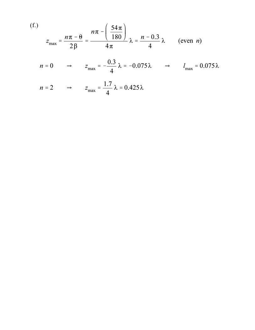
(f.)

Lossy Transmission Lines

The general transmission line equations (defined in terms of a

complex propagation constant) must be used when dealing with lossy lines.

The general transmission line equations are

The reflection coefficient for a lossy transmission line may be determined

by replacing each jâ term with ã which gives

In a similar fashion, the input impedance of a terminated lossy transmission

line is

Most transmission lines are designed with materials which produce small

losses (low loss lines). The general expressions for the characteristic

impedance and propagation constant of a lossy transmission line may be

simplified somewhat for a low-loss line.

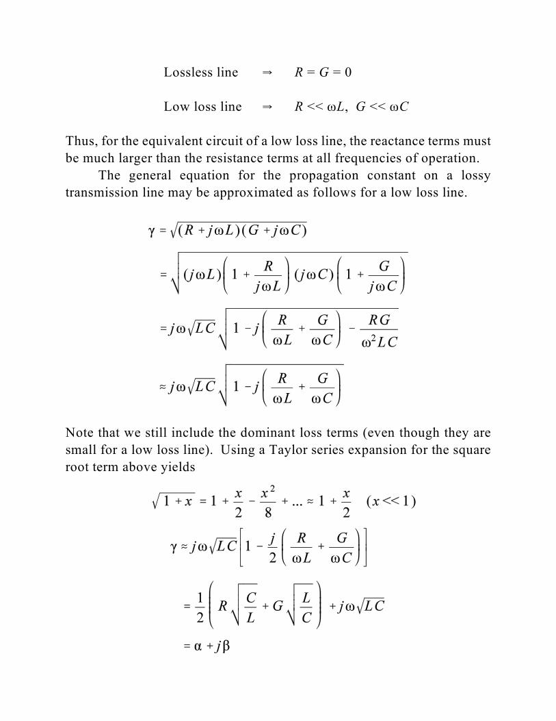
Lossless line Y R = G = 0

Low loss line Y R << ùL, G << ùC

Thus, for the equivalent circuit of a low loss line, the reactance terms must

be much larger than the resistance terms at all frequencies of operation.

The general equation for the propagation constant on a lossy

transmission line may be approximated as follows for a low loss line.

Note that we still include the dominant loss terms (even though they are

small for a low loss line). Using a Taylor series expansion for the square

root term above yields

Using the same approximations for the characteristic impedance, we find

The power level delivered to the load is lower than that delivered to

the transmission line input due to the line losses. The line losses can be

determined by calculating the difference in these power levels. The voltage

and current at the load are

The power delivered to the load is

The voltage and current at the input to the transmission line are

The power delivered to the input of the transmission line

The power lost in the transmission line is

Distortionless Transmission Line

On a lossless transmission line, the propagation constant is purely

imaginary and given by

The phase velocity on the lossless line is

Note that the phase constant which varies linearly with frequency produces

a constant phase velocity (independent of frequency) so that all frequencies

propagate along the lossless transmission line at the same velocity. From

Fourier theory, we know that any time-domain signal may be represented

as a weighted sum of sinusoids. Thus, signals transmitted along a lossless

transmission line will suffer no distortion since all of the frequency

components propagate at the same velocity. When the phase velocity of a

transmission line is a function of frequency, signals will become distorted

as different components of the signal arrive at different times. This effect

is called dispersion.

For the low-loss line, using the appropriate approximations, we found

which implies that the phase velocity on a low loss line is near constant.

However, the small variations in the phase velocity on a low loss line may

produce significant distortion if the line is very long.

There is a special case of lossy line with the linear phase constant that

produces a distortionless line. A transmission line is a distortionless line

if the per-unit-length parameters satisfy

Inserting the per-unit-length parameter relationship into the general

equation for the propagation constant on a lossy line gives

Although the shape of the signal is not distorted, the signal will suffer

attenuation as the wave propagates along the line since the distortionless

line is a lossy transmission line. Note that the attenuation constant for a

distortionless transmission line is also independent of frequency. If this

were not true, the signal would suffer distortion due to different frequencies

being attenuated by different amounts.

In the previous derivation, we have assumed that the per-unit-length

parameters of the transmission line are independent of frequency. This is

also an approximation that depends on the spectral content of the

propagating signal. For very wideband signals, the attenuation and phase

constants will, in general, be functions of frequency.

For most practical transmission lines, we find that RC > GL. In order

to satisfy the distortionless line requirement, series loading coils are

typically placed periodically along the line to increase L.

Perturbation Method for Determining Attenuation

Given only a forward wave propagating along a low loss transmission

line, the voltage and current of the wave may be written as

The power flow as a function of position along the transmission line is

given by

lThe power loss per unit length along the transmission line [P (z)] may

be written as

Solving for the attenuation constant gives

Since the fields of a low loss transmission line are very close to those of a

lossless line, we may use the lossless line fields to calculate the power loss

per unit length (perturbation method). Note that power P(z) and the power

lloss per unit length P (z) may be evaluated at any point on the transmission

line. The perturbation method allows for the calculation of the attenuation

constant using the transmission line fields rather than using the per-unit-

length parameters in the general propagation constant formula.

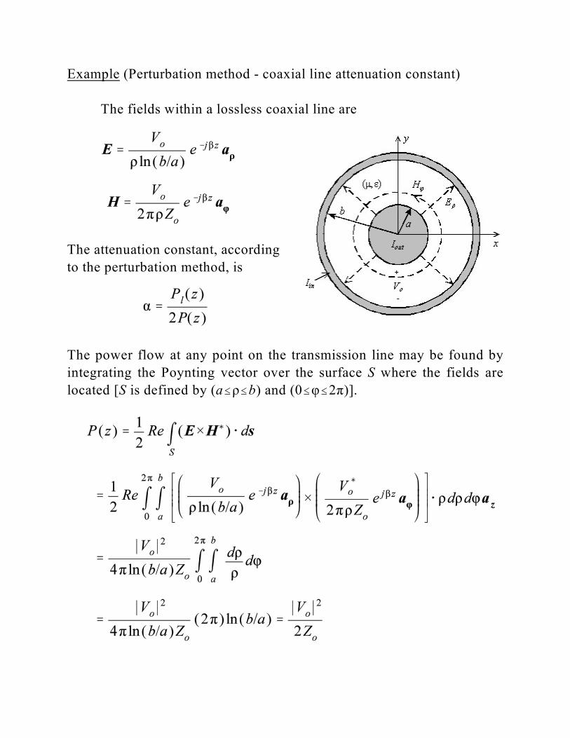
Example (Perturbation method - coaxial line attenuation constant)

The fields within a lossless coaxial line are

The attenuation constant, according

to the perturbation method, is

The power flow at any point on the transmission line may be found by

integrating the Poynting vector over the surface S where the fields are

located [S is defined by (a#ñ#b) and (0#ö#2ð)].

Assuming that the dielectric and magnetic losses are negligible, the power

loss per unit length in the conductors of the coaxial line is given by

si sowhere J and J are the surface currents on the inner and outer conductors

si sowhile R and R are the surface resistances of the inner and outer

iconductors. The surface S on the inner conductor is defined by ñ=a,

o0#ö#2ð, and 0#z#l while the surface S on the outer conductor is defined

by ñ=b, 0#ö#2ð, and 0#z#l. Using the surface impedance approx-imation,

the surface current on a good conductor is approximately that on a PEC

which may be written as

Thus, we may replace the surface currents in the power loss per unit length

equation by the surface magnetic fields associated with a lossless coaxial

line. The power loss per unit length is then

ti towhere H and H are the tangential magnetic fields on the surface of the

inner and outer conductors. If the inner and outer conductors are the same

material, then

Evaluation of the integrals in the power loss per unit length expression

yields

cThe attenuation constant due to conductor loss (á ) on the coaxial line

becomes

s sThe surface resistance (R ) of the conductors is related to the skin depth (ä )

by

oFor RG-59 coaxial cable (Z = 75 Ù, copper conductors, ó = 5.8 × 10 É/m,7

oa = 0.292 mm, b = 1.854 mm, ì = ì ) at 500 MHz,

s cR = 5.83 × 10 Ù, á = 0.0245 Np/m!3

Manufacturers normally specify the transmission line attenuation factor in

units of dB/m as opposed to Np/m. The conversion factor between the two

units is determined below.

nepWith á defined in Np/m (á ), the transmission line voltage attenuation is

dBWith á defined in dB/m (á ), the transmission line voltage attenuation is

Equating the two expressions yields

For the RG-59 coaxial line,

Wheeler Incremental Inductance Rule

By noting that the conductor loss in a transmission line can be related

to the small change in the transmission line inductance due to the

penetration of the fields into the conductors, Wheeler derived an equation

for the transmission line conductor loss in terms of the change in the

characteristic impedance. The result of the Wheeler incremental inductance

rule may be written as

s owhere is R the surface resistance of the conductor, Z is the characteristic

impedance of the transmission line assuming perfect conductors, ç is the

intrinsic impedance of the dielectric between the conductors, and l defines

the direction into the conductors. The characteristic impedance of the

lossless coaxial transmission line is given by

The derivative term in the attenuation factor expression is

The attenuation factor due to conductor loss in the coaxial transmission line

becomes

which is identical to the result found using the perturbation method.