transmission strategies for wireless energy harvesting …€¦ · transmission strategies for...
TRANSCRIPT
Departament de Teoriadel Senyal i Comunicac ions
Transmission strategiesfor wireless energy harvesting nodes
By
Maria Gregori Casas
Submitted to the Universitat Politecnica de Catalunya (UPC)
in partial fulfillment of the requirements for the degree of
DOCTOR OF PHILOSOPHY
Barcelona, June 2014
Supervised by Dr. Miquel Payaro i LlisterriPhD program on Signal Theory and Communications


Als meus pares, Pere i Anna,
us estare eternament agraıda
per transmetre’m els vostres valors, amor i suport.


This work has been supported by the CTTC under the 2010 PhD scholarship program and by the Catalan
Government (AGAUR) under the grants:
2011FI B 00956, 2012FI B1 00173, and 2013FI B2 00075.


Abstract
Over the last few decades, transistor miniaturization has enabled a tremendous increase in the
processing capability of commercial electronic devices, which, combined with the reduction of
production costs, has tremendously fostered the usage of the Information and Communications
Technologies (ICTs) both in terms of number of users and required data rates. In turn, this has
led to a tremendous increment in the energetic demand of the ICT sector, which is expected
to further grow during the upcoming years, reaching unsustainable levels of greenhouse gas
emissions as reported by the European Council.
Additionally, the autonomy of battery operated devices is getting reduced year after year
since battery technology has not evolved fast enough to cope with the increase of energy con-
sumption associated to the growth of the node’s processing capability.
Energy harvesting, which is known as the process of collecting energy from the environ-
ment by different means (e.g., solar cells, piezoelectric generators, etc.), has become a potential
technology to palliate both of these problems. However, when energy harvesting modules are
placed in wireless communication devices (e.g., sensor nodes or hand-held devices), traditional
transmission strategies are no longer applicable because the temporal variations of the node’s
energy availability must be carefully accounted for in the design.
Apart from not considering energy harvesting, traditional transmission strategies assume
that the transmission radiated power is the unique energy sink in the node. This is a reasonable
assumption when the transmission range is large, but it no longer holds for low consumption
devices such as sensor nodes that transmit to short distances. As a result, classical transmission
strategies become suboptimal in short-range communications with low consumption devices
and new strategies should be investigated.
Consequently, in this dissertation we investigate and design transmission strategies for
Wireless Energy Harvesting Nodes (WEHNs) by paying a special emphasis on the different
sinks of energy consumption at the transmitter(s).
First, we consider a finite battery WEHN operating in a point-to-point link through a static
vii

channel and derive the transmission strategy that minimizes the transmission completion time
of a set of data packets that become available dynamically over time. The transmission strategy
has to satisfy causality constrains in data transmission and energy consumption, which impose
that the node cannot transmit data that is not yet available nor consume energy that has not yet
been harvested.
Second, we consider a WEHN that has an infinite backlog of data to be transmitted through
a point-to-point link in a time-varying linear vector Gaussian channel and study the linear
precoding strategy that maximizes the mutual information given an arbitrary distribution of the
input symbols while satisfying the Energy Causality Constraints (ECCs) at the transmitter.
Next, apart from the transmission radiated power, we take into account additional energy
sinks in the power consumption model and analyze how these energy sinks affect to the trans-
mission strategy that maximizes the mutual information achieved by a WEHN operating in a
point-to-point link.
Finally, we consider multiple transmitter and receiver pairs sharing a common channel and
investigate a distributed power allocation strategy that aims at maximizing the network sum-
rate by taking into account the energy availability in the different transmitters and a generalized
power consumption model.
viii

Resum
Durant les ultimes decades, la miniaturitzacio del transistor i la reduccio dels seus costos de
fabricacio han provocat un augment substancial del nombre de terminals de comunicacions i
del trafic de dades requerit per aquests dispositius. Aixı doncs, el consum energetic del sector
de les Tecnologies de la Informacio i Comunicacions ha incrementat notablement. A mes a
mes, s’espera que aquest consum segueixi creixent durant els propers anys arribant a nivells
insostenibles d’emissions de gasos d’efecte hivernacle segons ha informat el Consell Europeu.
D’altra banda, la tecnologia de les bateries no ha evolucionat suficientment rapid com per
fer front a l’augment del consum energetic associat al creixement de la capacitat de proces-
sament dels dispositius. Aixo ha ocasionat que l’autonomia dels dispositius que operen amb
bateries empitjori any rere any.
Les energies renovables (per exemple, energia solar, cinetica, etc.) s’han convertit en una
solucio potencial per pal·liar aquests dos problemes. No obstant aixo, quan els dispositius de
comunicacio sense fils incorporen moduls de captacio d’energies renovables, les estrategies
tradicionals de transmissio deixen de ser valides, ja que les variacions temporals de la disponi-
bilitat d’energia en el dispositiu han de ser considerades en el disseny.
A mes a mes, les estrategies de transmissio tradicionals assumeixen que la potencia radiada
es l’unica font de consum energetic del node. Aquesta es una suposicio raonable per distancies
de transmissio llargues, pero deixa de ser valida quan es consideren dispositius de baix consum
que transmeten en distancies curtes. Com a resultat, les estrategies de transmissio classiques
son suboptimes en comunicacions de curt abast amb dispositius de baix consum i per aixo,
s’han d’investigar noves estrategies.
En consequencia, en aquesta tesi doctoral s’investiguen i es dissenyen noves estrategies
de transmissio per nodes sense fils que operen amb energies renovables (WEHN) posant un
emfasi especial en les diferents fonts de consum d’energia en el transmissor.
En primer lloc, la tesi investiga l’estrategia de transmissio en un enllac punt a punt a traves
d’un canal estatic que minimitza el temps de transmissio d’un conjunt de paquets de dades que
ix

s’adquireixen al llarg del temps. L’estrategia de transmissio ha de satisfer les limitacions per
causalitat en la transmissio de dades i en el consum d’energia les quals imposen que el node
no pot transmetre dades que no han estat encara obtingudes o utilitzar energia que encara no ha
estat adquirida.
En segon lloc, es considera un WEHN que sempre disposa de dades per a transmetre
a traves d’un enllac punt a punt en un canal lineal Gaussia amb variacions temporals. En
aquest escenari i, tambe, donada una distribucio arbitraria dels sımbols d’entrada, s’estudia
l’estrategia de precodificacio lineal que maximitza la informacio mutua alhora que satisfa la
causalitat d’energia en el transmissor.
A continuacio, a part de la potencia radiada en transmissio, s’inclouen en el model de
consum energetic els costos d’activacio per acces al canal i per portadora. Donat aquest model,
s’analitza com aquestes fonts de consum addicionals afecten a l’estrategia de transmissio que
maximitza la informacio mutua d’un WEHN que opera en un enllac punt a punt.
Finalment, la tesi considera diversos parells transmissor i receptor que comparteixen un
canal comu i investiga una estrategia d’assignacio de potencia distribuıda la qual te com a
objectiu maximitzar la suma de les taxes de transmissio dels diferents nodes tenint en compte la
disponibilitat energetica en cada transmissor que esta basada en un model de consum energetic
generalitzat.
x

Acknowledgements
It was four years ago, but it seems like it was only yesterday that I entered the Centre Tecnologic
de Telecomunicacions de Catalaunya (CTTC) for the first time and Laura Casaus showed me
the different offices and labs introducing me to my future colleagues; simply, time flies when
one enjoys every single moment of every single day. Of course, all this joy is due to the great
companions and friends at CTTC. In the following lines, I will try to thank you all; I hope I do
not forget anyone. :)
First and foremost, I would like to thank my PhD advisor, Dr. Miquel Payaro i Llisterri,
for his valuable help, suggestions, comments, and constructive criticisms that have greatly
helped me to keep learning day after day. Miquel introduced me into the exciting worlds
of convex optimization and linear precoder design and taught me the preciseness and rigor
required in all the technical derivations. I also want to thank Miquel for being always flexible
and comprehensive allowing me to select and study the problems for which I felt more interest.
In short, I extremely appreciate Miquel’s support both in professional and personal terms.
I also want to thank Professor Daniel Perez Palomar for giving me the opportunity to join
his research lab in the Hong Kong University of Science and Technology, treating me as one
more of his PhD students, and letting me assist to his course on Convex Optimization. During
this internship, I really consolidated several concepts of convex optimization and learned many
approaches to solve nonconvex optimization problems.
Additionally, I thank Jesus Gomez, Kostas Stamatiou, Antonio Pascual-Iserte, and Miquel
Calvo for reviewing part of this thesis.
Next, I would like to thank the CTTC both for the received funding and for giving me the
opportunity to carry out my PhD thesis in such good conditions and work environment.
This amazing work environment is created by the great people working at CTTC; I thank
all of them. Specially, I would like to thank the colleagues that have partially or fully over-
lapped their PhD studies with mine:
xi

• First, I thank the guys in the coo- wait for it -lest office ever: Jaume Ferragut for always
bringing up funny debates; Ana Maria Galindo for broadcasting happiness and joy in
the office, making it a funny Q-learning place; Moises Espinosa for his interesting early
morning talks; the casanova of the lab, Angelos Antonopoulos, for constantly making
fun of me; Pol Blasco for the funny terrace parties; Musbah Shaat, Vahid Joroughi and
Alessandro Acampora for sharing with me a bit of their culture; Laia Nadal for being
such a good person; Jessica Moysen for teaching us funny Mexican words that make us
laugh for weeks; and Giussepe Cocco for his tremendous sense of humor.
• Second, the guys in the coo- wait for it -kie office: Inaki Estella, Andrea Bartoli, Daniel
Sacristan, Javier Arribas, Anica Bukva, Lazar Berbakov, Tatjana Predojev, Biljana Bo-
jovic, Kyriaki Niotaki, Juan Manuel Castro, and Miquel Calvo.
• Finally, I also want to thank Onur Tan, Konstantinos Ntontin, Miguel Angel Vazquez,
Adria Gusi, Javier Rubio, Aleksandar Brankovic, Rakesh Kumar, Italo Atzeni and the
Greek gang leaded by Alexandra Bousia.
Apart from the PhD students, I would like to thank all the players in the PMT padel
tournament for the funny weekly matches; specially, I thank Edu Dıaz for the organization.
Tambe vull agraır als meus amics i companys de viatge durant tots aquests anys. En primer
lloc, a Judit Aliberas, Aida Abiad, Laia Simo, Adria Barbosa, Carmina Gil i Eric Juan ja que
cada moment que aconseguim passar els set junts es sempre unic i innolvidable. En segon
lloc, a la Gemma Roger i en Lluıs Pons pel vostre suport i amistat durant la meva estada a
Hong Kong. Tot seguit, a en Lluıs Parcerisa i la Neus Roca (la nano-people), i a la resta del
Quelf-team, Emili Nogues, Ivan Pardina i Enric Pulido. A tot el grup de Valldemia, Montse
Damont, Griselda Abril, Nuria Farras, Laura Ricos, Lluıs Polo, Sandra Castane, Aurora Gil, i
Carla Alena amb qui sempre aconseguim estar al dia. A la Gemma Molina i el Christian Roldan
per la vostra amistat al llarg dels anys. Als konjos etıops, Clara Macia, Laura Gonzalez, Jesus
Berdun, Llorenc Mercer i Kaja Miko ja que quan ens reunim es impossible parar de riure.
Per ultim, vull agraır i dedicar aquesta tesi a la meva famılia: Pere Gregori, Ana Casas
i Xavi Gregori; Angelina Gomez i Pere Casas; Pilar Isla i Pere Gregori; Jordi Gregori; Nina
Casas, Jordi Figueras, Marc Figueras i Aina Figueras; Joan Carles Gregori, Marta Palacios,
Oriol Gregori i Sergi Gregori. Sense el vostre amor i suport aquesta tesi no seria possible.
xii

List of Publications
Journals
[J1] M. Gregori, M. Payaro, G. Scutari, and D. P. Palomar, “Sum-rate maximization for en-
ergy harvesting nodes with a generalized power consumption model,” in preparation,
2014.
[J2] M. Gregori and M. Payaro, “On the optimal resource allocation for a wireless energy
harvesting node considering the circuitry power consumption,” accepted in IEEE Trans.
on Wireless Communications, Jun. 2014.
[J3] M. Gregori and M. Payaro, “On the precoder design of a wireless energy harvesting
node in linear vector Gaussian channels with arbitrary input distribution,” IEEE Trans.
on Communications, vol. 61, no. 5, pp. 1868–1879, May 2013.
NEWCOM# 2013 Best young researcher’s paper award.Committee:
Muriel Medard, MIT Boston, USA
Petar M. Djuric, Stony Brook University, USA
Bjorn Ottersten, University of Luxembourg, Luxembourg.
[J4] M. Gregori and M. Payaro, “Energy-efficient transmission for wireless energy harvesting
nodes,” IEEE Trans. on Wireless Communications, vol. 12, no. 3, pp. 1244–1254, Mar.
2013.
International Conferences
[C1] M. Gregori and M. Payaro, “Multiuser communications with energy harvesting transmit-
ters,” in Proceedings of the IEEE International Conference on Communications (ICC),
2014.
xiii

[C2] M. Gregori, A. Pascual-Iserte, and M. Payaro, “Mutual information maximization for a
wireless energy harvesting node considering the circuitry power consumption,” in Pro-
ceedings of the IEEE Wireless Communications and Networking Conference (WCNC),
Apr. 2013, pp. 4238–4243.
[C3] M. Gregori and M. Payaro, “Throughput maximization for a wireless energy harvesting
node considering the circuitry power consumption,” in Proceedings of the IEEE Vehicu-
lar Technology Conference (VTC Fall), Sep. 2012, pp. 1–5.
[C4] M. Gregori and M. Payaro, “Optimal power allocation for a wireless multi-antenna en-
ergy harvesting node with arbitrary input distribution,” in Proceedings of the IEEE Inter-
national Conference on Communications (ICC), Jun. 2012, pp. 5794 –5798.
[C5] M. Gregori and M. Payaro, “Efficient data transmission for an energy harvesting node
with battery capacity constraint,” in Proceedings of the IEEE Global Telecommunications
Conference (GLOBECOM), Dec. 2011, pp. 1–6.
[C6] M. Payaro, M. Gregori, and D. P. Palomar, “Yet another entropy power inequality with
an application,” in Proceedings of the IEEE International Conference on Wireless Com-
munications and Signal Processing (WCSP), Nov. 2011, pp. 1–5.
xiv
Contents
1 Introduction 1
1.1 Motivation . . . . . . . . . . . . . . . . . . . . . . . . . . . . . . . . . . . . . 1
1.2 Outline of the dissertation and research contributions . . . . . . . . . . . . . . 4
2 Background and state of the art 9
2.1 Characteristics of wireless energy harvesting nodes . . . . . . . . . . . . . . . 9
2.1.1 Energy sources and power harvesting profile . . . . . . . . . . . . . . 12
2.1.2 The communications channel . . . . . . . . . . . . . . . . . . . . . . 18
2.1.3 Offline and online transmission strategies . . . . . . . . . . . . . . . . 20
2.1.4 Sources of power consumption . . . . . . . . . . . . . . . . . . . . . . 21
2.1.5 Figure of merit and constraints . . . . . . . . . . . . . . . . . . . . . . 22
2.1.6 Linear transmitter design problem formulation . . . . . . . . . . . . . 24
2.2 State of the art on transmission strategies
for non-harvesting nodes . . . . . . . . . . . . . . . . . . . . . . . . . . . . . 25
2.2.1 Maximization of the mutual information . . . . . . . . . . . . . . . . . 25
2.2.2 Energy consumption minimization . . . . . . . . . . . . . . . . . . . . 31
2.3 State of the art on transmission strategies for WEHNs . . . . . . . . . . . . . . 33
2.3.1 Directional Water-Filling (DWF) . . . . . . . . . . . . . . . . . . . . . 33
2.3.2 Other transmission strategies for WEHNs . . . . . . . . . . . . . . . . 35
3 Transmission completion time minimization for a WEHN 39
3.1 Introduction . . . . . . . . . . . . . . . . . . . . . . . . . . . . . . . . . . . . 39
3.2 Problem formulation . . . . . . . . . . . . . . . . . . . . . . . . . . . . . . . 41
3.3 Properties of the optimal solution . . . . . . . . . . . . . . . . . . . . . . . . . 47
3.3.1 Constraints mapping into the data domain for a given pool . . . . . . . 49
xv
Contents
3.4 Optimal data departure curve construction . . . . . . . . . . . . . . . . . . . . 52
3.5 Results . . . . . . . . . . . . . . . . . . . . . . . . . . . . . . . . . . . . . . . 54
3.6 Conclusions . . . . . . . . . . . . . . . . . . . . . . . . . . . . . . . . . . . . 55
3.A Appendix . . . . . . . . . . . . . . . . . . . . . . . . . . . . . . . . . . . . . 56
3.A.1 Proof of Lemma 3.2 . . . . . . . . . . . . . . . . . . . . . . . . . . . 56
3.A.2 Rate change characterization . . . . . . . . . . . . . . . . . . . . . . . 58
3.A.3 The algorithm . . . . . . . . . . . . . . . . . . . . . . . . . . . . . . . 59
4 On the precoder design of a wireless energy harvesting node in linear vector Gaus-sian channels with arbitrary input distribution 65
4.1 Introduction . . . . . . . . . . . . . . . . . . . . . . . . . . . . . . . . . . . . 65
4.2 System model . . . . . . . . . . . . . . . . . . . . . . . . . . . . . . . . . . . 67
4.3 Throughput maximization problem . . . . . . . . . . . . . . . . . . . . . . . . 69
4.4 The MIMO Mercury Water-Flowing solution . . . . . . . . . . . . . . . . . . 73
4.5 MIMO Mercury Water-Flowing offline algorithms . . . . . . . . . . . . . . . . 76
4.5.1 Non Decreasing water level Algorithm (NDA) . . . . . . . . . . . . . 77
4.5.2 Forward Search Algorithm (FSA) . . . . . . . . . . . . . . . . . . . . 77
4.5.3 Optimality and performance characterization of the
offline algorithms . . . . . . . . . . . . . . . . . . . . . . . . . . . . . 78
4.6 Online algorithm . . . . . . . . . . . . . . . . . . . . . . . . . . . . . . . . . 79
4.7 Results . . . . . . . . . . . . . . . . . . . . . . . . . . . . . . . . . . . . . . . 81
4.7.1 Results on the MIMO Mercury Water-Flowing solution . . . . . . . . . 81
4.7.2 Results on the algorithms’ performance . . . . . . . . . . . . . . . . . 84
4.8 Conclusions . . . . . . . . . . . . . . . . . . . . . . . . . . . . . . . . . . . . 85
4.A Appendix . . . . . . . . . . . . . . . . . . . . . . . . . . . . . . . . . . . . . 86
4.A.1 Proof of Lemma 4.1 . . . . . . . . . . . . . . . . . . . . . . . . . . . 86
4.A.2 Proof of Lemma 4.2 . . . . . . . . . . . . . . . . . . . . . . . . . . . 86
4.A.3 Proof of Lemma 4.3 . . . . . . . . . . . . . . . . . . . . . . . . . . . 87
4.A.4 Proof of Theorem 4.1 . . . . . . . . . . . . . . . . . . . . . . . . . . . 89
4.A.5 Computational complexity of the algorithms . . . . . . . . . . . . . . 89
4.A.6 Properties of the reduction matrix . . . . . . . . . . . . . . . . . . . . 95
5 On the optimal resource allocation for a wireless energy harvesting node consid-
xvi
Contents
ering the circuitry power consumption 97
5.1 Introduction . . . . . . . . . . . . . . . . . . . . . . . . . . . . . . . . . . . . 97
5.2 System model and problem formulation . . . . . . . . . . . . . . . . . . . . . 99
5.3 Offline resource allocation . . . . . . . . . . . . . . . . . . . . . . . . . . . . 104
5.3.1 Integer relaxation . . . . . . . . . . . . . . . . . . . . . . . . . . . . . 104
5.3.2 Duality . . . . . . . . . . . . . . . . . . . . . . . . . . . . . . . . . . 110
5.3.3 The Boxed Water-Flowing interpretation . . . . . . . . . . . . . . . . 115
5.4 Online resource allocation . . . . . . . . . . . . . . . . . . . . . . . . . . . . 118
5.5 Simulation results . . . . . . . . . . . . . . . . . . . . . . . . . . . . . . . . . 120
5.6 Conclusions . . . . . . . . . . . . . . . . . . . . . . . . . . . . . . . . . . . . 124
5.A Appendix . . . . . . . . . . . . . . . . . . . . . . . . . . . . . . . . . . . . . 125
5.A.1 Proof of Lemma 5.1 . . . . . . . . . . . . . . . . . . . . . . . . . . . 125
5.A.2 Proof of Lemma 5.2 . . . . . . . . . . . . . . . . . . . . . . . . . . . 126
5.A.3 Proof of Proposition 5.1 . . . . . . . . . . . . . . . . . . . . . . . . . 126
5.A.4 Proof of Lemma 5.3 . . . . . . . . . . . . . . . . . . . . . . . . . . . 127
5.A.5 Proof of Lemma 5.4 . . . . . . . . . . . . . . . . . . . . . . . . . . . 128
5.A.6 Proof of Proposition 5.2 . . . . . . . . . . . . . . . . . . . . . . . . . 130
5.A.7 Derivation of the cutoff water level . . . . . . . . . . . . . . . . . . . 132
6 Sum-rate maximization in multiuser communications with WEHNs considering ageneralized power consumption model 133
6.1 Introduction . . . . . . . . . . . . . . . . . . . . . . . . . . . . . . . . . . . . 133
6.2 System model and problem formulation . . . . . . . . . . . . . . . . . . . . . 136
6.3 Approximations of the step function . . . . . . . . . . . . . . . . . . . . . . . 140
6.3.1 Smooth approximation of the step function . . . . . . . . . . . . . . . 140
6.3.2 Convex approximation of the smooth step function . . . . . . . . . . . 143
6.4 The Iterative Smooth and Convex approximation Algorithm (ISCA) . . . . . . 144
6.4.1 The inner loop: Nonconvex optimization of smooth problems with
Successive Convex Approximation (SCA) . . . . . . . . . . . . . . . . 146
6.4.2 Determining a feasible initial point for the inner loop. . . . . . . . . . . 149
6.4.3 Convergence of the feasible sets and distributed implementation . . . . 150
6.5 The ISCA algorithm for C2t . . . . . . . . . . . . . . . . . . . . . . . . . . . . . 151
6.6 Results . . . . . . . . . . . . . . . . . . . . . . . . . . . . . . . . . . . . . . . 154
xvii

Contents
6.7 Conclusions . . . . . . . . . . . . . . . . . . . . . . . . . . . . . . . . . . . . 157
6.A Appendix . . . . . . . . . . . . . . . . . . . . . . . . . . . . . . . . . . . . . 158
6.A.1 Proof of Lemma 6.2 . . . . . . . . . . . . . . . . . . . . . . . . . . . 158
6.A.2 Proof of Lemma 6.3 . . . . . . . . . . . . . . . . . . . . . . . . . . . 159
6.A.3 Proof of Lemma 6.4 . . . . . . . . . . . . . . . . . . . . . . . . . . . 160
7 Thesis conclusions and future work 161
7.1 Conclusions . . . . . . . . . . . . . . . . . . . . . . . . . . . . . . . . . . . . 161
7.2 Future Work . . . . . . . . . . . . . . . . . . . . . . . . . . . . . . . . . . . . 163
xviii

List of acronyms
AWGN Additive White Gaussian Noise
BER Bit Error Rate
CDMA Code Division Multiple Access
CSI Channel State Information
CWF Classical Water-Filling
DAI Data Arrival Information
DCC Data Causality Constraint
DMT Discrete Multi-Tone
DSL Digital Subscriber Line
DWF Directional Water-Filling
EBS Empty Buffers Strategy
ECC Energy Causality Constraint
EH Energy Harvesting
EHI Energy Harvesting Information
FSA Forward Search Algorithm
GSM Global System for Mobile communications
HgWF Mercury/Water-Filling
HgWFA Mercury/Water-Filling Algorithm
xix

ICT Information and Communications Technology
IFFT Inverse Fast Fourier Transform
i.i.d. independent and identically distributed
ISCA Iterative Smooth and Convex approximation Algorithm
IV Indicator Variable
KKT Karush–Kuhn–Tucker
MIMO Multiple-Input Multiple-Output
MMSE Minimum Mean-Square Error
MSE Mean-Square Error
MUI MultiUser Interference
NDA Non Decreasing water level Algorithm
OFDM Orthogonal Frequency Division Multiplexing
QoS Quality of Service
RF Radio Frequency
RFID Radio Frequency IDentification
SCA Successive Convex Approximation
SINR Signal to Interference plus Noise Ratio
SISO Single-Input Single-Output
SNR Signal to Noise Ratio
SSA Successive Smooth Approximation
WEHN Wireless Energy Harvesting Node
WLAN Wireless Local Area Network
w.r.t. with respect to
xx

Notation
R,C,N The set of real, complex, and natural numbers, respectively.
R+ The set of nonnegative real numbers.
Rn,Rn+ The set of vectors of dimension n with entries in R and R+,
respectively.
Rn×m,Rn×m+ ,Cn×m The set of n×m matrices with entries in R, R+ and C , respectively.
x Scalar.
x Column vector.
X Matrix.
X Set.
||x|| Euclidian norm of the vector x, i.e.,√
xHx.
|X | Cardinality of the set X .
[x]n n-th component of the vector x.
[X]pq Element in the p-th row and q-th column of matrix X.
In Identity matrix of order n.
1n, 0n Column vector of n ones or zeros.
The dimension n might be omitted when it can be deduced from the
context.
(·)T Transpose operator.
(·)H Conjugate transpose operator.
Tr(·) Trace operator.
diag(X) Column vector that contains the diagonal elements of the matrix X.
Diag(x) Diagonal matrix where the diagonal entries are given by the vector x.
vec(X) Column vector that stacks the columns of X.
x = (xn)Nn=1 Column vector constructed by stacking vectors xn, i.e.,
x = [xT1 , . . . ,x
TN ]T.
df(x)dx Derivative of the scalar function f (x) with respect to (w.r.t.) x.
xxi
∂f(x,y)∂x
Partial derivative of the scalar function f (x, y) w.r.t. x.
∇xf(x) Gradient of the function f (x) w.r.t. x.
DXF Jacobian of the matrix function F w.r.t. the matrix variable X.∫ baf(x)dx Integral of f (x) w.r.t. x in the interval [a,b].
⊗ Kronecker product.
◦ Hadamard product.
[x]ba Projection of x in the interval [a, b].
[x]+ Projection of x into R+, i.e., max{0, x}.E{·} Expected value.
var{·} Variance.
≤,≥ Smaller and greater than or equal inequality, respectively.
�,� Componentwise smaller and greater than or equal inequality,
respectively.
arg Argument.
maximizex f(x) Maximize the objective function f(x) w.r.t. the optimization
variable x.
minimizex f(x) Minimize the objective function f(x) w.r.t. the optimization
variable x.
x? Optimal value of a given optimization problem.
max,min Pointwise maximum and minimum.
H`(·) Left continuous unit step function, i.e.,
H`(x) = 1 if x > 0 andH`(x) = 0, otherwise.
Hr(·) Right continuous unit step function, i.e.,
Hr(x) = 1 if x ≥ 0 andHr(x) = 0, otherwise.
Π(·) Unit pulse in the interval [0, 1], i.e.,
Π(x) = 1 if x ∈ [0, 1] and Π(x) = 0, otherwise.
W0(·) Positive branch of the Lambert function.
log(·) Natural logarithm.
logb(·) Base-b logarithm.
∩,∪ Intersection and union, respectively.
⊂,⊆ Proper subset and subset, respectively.
∼ Distributed according to.
≈ Approximately equal to.
B (n, q) Binomial distribution of parameters n and q.
CN (m,C) Complex circularly symmetric Gaussian vector distribution with
mean m and covariance matrix C.
N (m,σ2) Gaussian distribution with mean m and variance σ2.
xxii

Chapter 1Introduction
“The Information and Communications Technologies (ICTs) industry is in a unique
position to demonstrate leadership in reducing its footprint, through structural
change and innovation as well as by leading the way in identifying and creating
efficient solutions for other socio-economic sectors to follow.
...
This can be done for instance by replacing products with on-line services (e.g.
company newsletters), by moving business to the internet (e.g. costumer’s support),
by adopting new ways of working (tele-working and flexi-work enhanced by video-
conferencing and tele-presence tools) and by exploring the viability of using green
suppliers and energy from renewable resources.”
The European Comission [1].
1.1 Motivation
The discovery of the transistor in 1947 revolutionized the field of electronics, becoming the
fundamental component of current electronic devices. The transistor’s inventors John Bardeen,
Walter Brattain, and William Shockley were worldwide recognized with the Nobel Prize in
Physics in 1956.
A few years later, in 1965, Gordon Moore accurately predicted that the number of tran-
sistors that can be placed in an integrated circuit would double every two years [2]. Since
then, transistor miniaturization has enabled a tremendous increase in the processing capability
of commercial electronic devices, which combined with the reduction of production costs has
tremendously fostered the sales of electronic equipments. As a result, the usage of the ICTs
has exponentially grown during last years both in terms of number of users and required data
1
Chapter 1. Introduction
1990 1994 1994
Year
Disk capacity
CPU speed
Available RAM
Wireless transfer speed
Battery energy density
1996 1998 2000 2002
Imp
rove
me
nt
mu
ltip
le s
ince
19
90
1,000
100
10
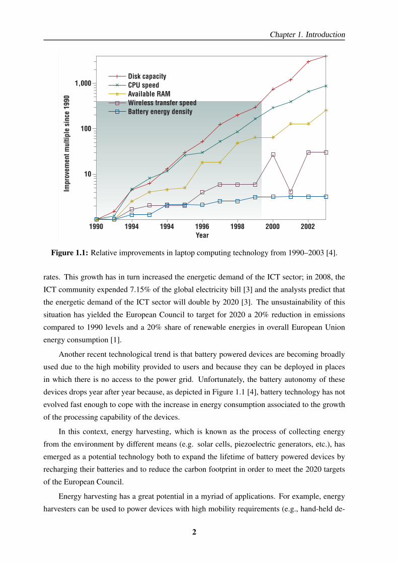
Figure 1.1: Relative improvements in laptop computing technology from 1990–2003 [4].
rates. This growth has in turn increased the energetic demand of the ICT sector; in 2008, the
ICT community expended 7.15% of the global electricity bill [3] and the analysts predict that
the energetic demand of the ICT sector will double by 2020 [3]. The unsustainability of this
situation has yielded the European Council to target for 2020 a 20% reduction in emissions
compared to 1990 levels and a 20% share of renewable energies in overall European Union
energy consumption [1].
Another recent technological trend is that battery powered devices are becoming broadly
used due to the high mobility provided to users and because they can be deployed in places
in which there is no access to the power grid. Unfortunately, the battery autonomy of these
devices drops year after year because, as depicted in Figure 1.1 [4], battery technology has not
evolved fast enough to cope with the increase in energy consumption associated to the growth
of the processing capability of the devices.
In this context, energy harvesting, which is known as the process of collecting energy
from the environment by different means (e.g. solar cells, piezoelectric generators, etc.), has
emerged as a potential technology both to expand the lifetime of battery powered devices by
recharging their batteries and to reduce the carbon footprint in order to meet the 2020 targets
of the European Council.
Energy harvesting has a great potential in a myriad of applications. For example, energy
harvesters can be used to power devices with high mobility requirements (e.g., hand-held de-
2
1.1. Motivation
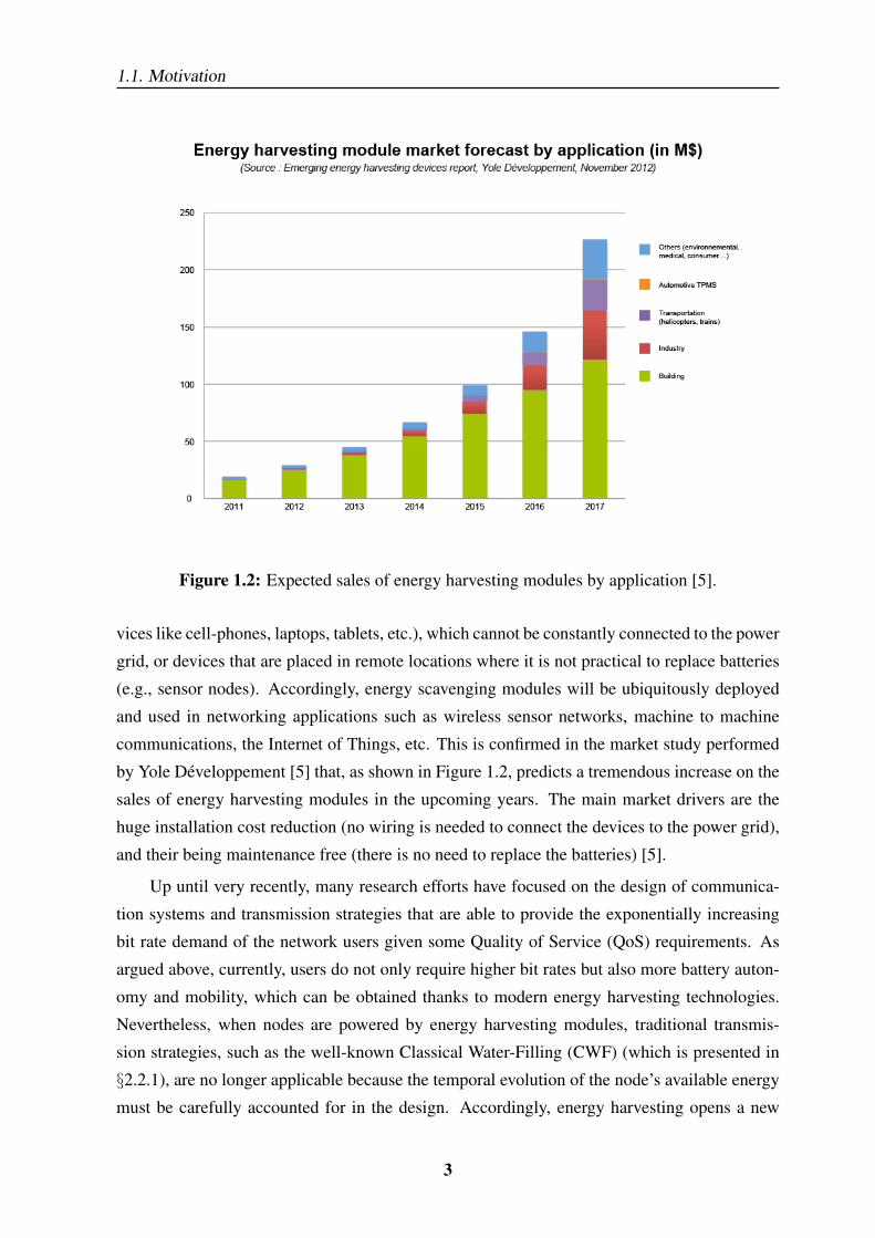
Figure 1.2: Expected sales of energy harvesting modules by application [5].
vices like cell-phones, laptops, tablets, etc.), which cannot be constantly connected to the power
grid, or devices that are placed in remote locations where it is not practical to replace batteries
(e.g., sensor nodes). Accordingly, energy scavenging modules will be ubiquitously deployed
and used in networking applications such as wireless sensor networks, machine to machine
communications, the Internet of Things, etc. This is confirmed in the market study performed
by Yole Developpement [5] that, as shown in Figure 1.2, predicts a tremendous increase on the
sales of energy harvesting modules in the upcoming years. The main market drivers are the
huge installation cost reduction (no wiring is needed to connect the devices to the power grid),
and their being maintenance free (there is no need to replace the batteries) [5].
Up until very recently, many research efforts have focused on the design of communica-
tion systems and transmission strategies that are able to provide the exponentially increasing
bit rate demand of the network users given some Quality of Service (QoS) requirements. As
argued above, currently, users do not only require higher bit rates but also more battery auton-
omy and mobility, which can be obtained thanks to modern energy harvesting technologies.
Nevertheless, when nodes are powered by energy harvesting modules, traditional transmis-
sion strategies, such as the well-known Classical Water-Filling (CWF) (which is presented in
§2.2.1), are no longer applicable because the temporal evolution of the node’s available energy
must be carefully accounted for in the design. Accordingly, energy harvesting opens a new
3
Chapter 1. Introduction
research paradigm for the design of transmission strategies.
Additionally, classical transmission strategies generally consider that the transmission ra-
diated power is the unique source of energy consumption of the node. This is a reasonable
assumption when the transmission range is large, but it no longer holds for low consumption
devices such as sensor nodes that transmit to short distances. As a result, classical transmission
strategies become suboptimal in short-range communications with low consumption devices
and new strategies should be investigated.
To summarize all what has been said above, the study and design of transmission strategies
for energy harvesting nodes is required in order to enlarge the autonomy of battery operated
devices and, at the same time, to reduce the carbon footprint of the ICT community; it is key
that these transmission strategies not only account for the transmission radiated power but also
for other relevant sources of energy consumption.
1.2 Outline of the dissertation and research contributions
This dissertation considers transmitter nodes equipped with energy harvesting modules, which
palliate the battery autonomy problem, and investigates transmission strategies that take into
account the energy availability variations in the node. More precisely, the thesis studies theoret-
ical bounds on the best achievable performance in different scenarios as well as practical trans-
mission strategies that can be implemented in Wireless Energy Harvesting Nodes (WEHNs).
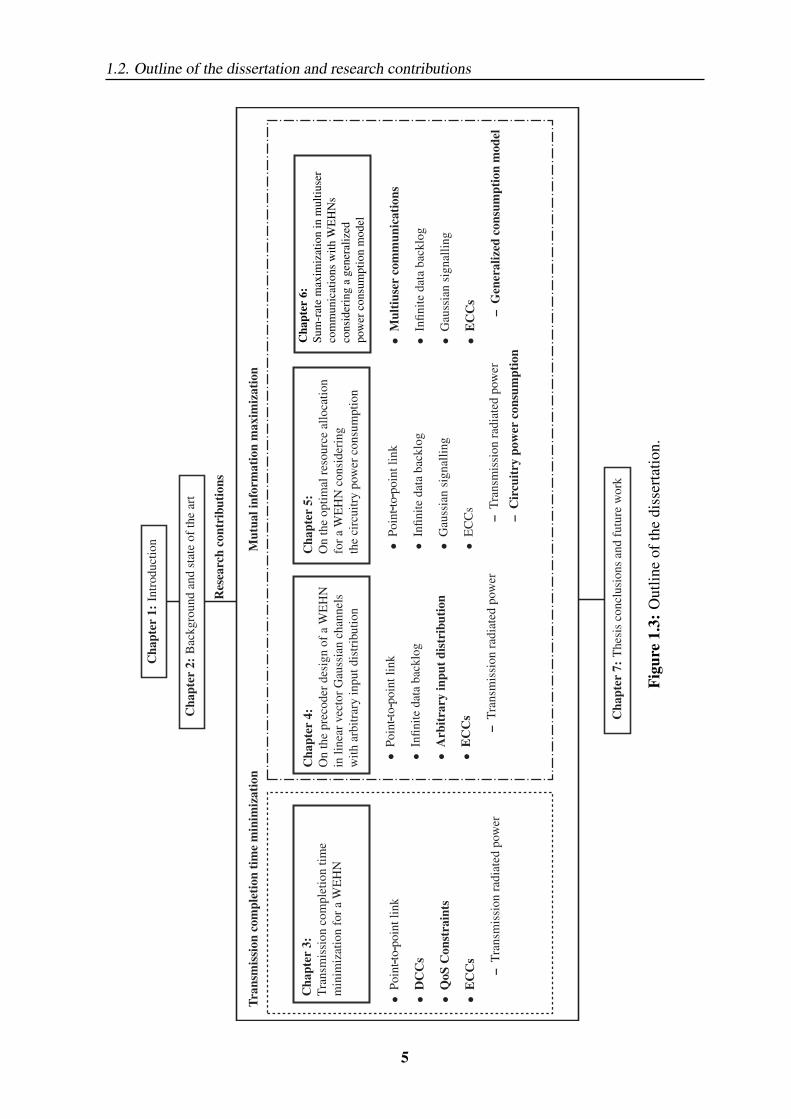
As depicted in Figure 1.3, the dissertation is structured in seven chapters and two different
performance measures are considered: (i) transmission completion time minimization, which
is studied in Chapter 3; and (ii) mutual information maximization, which is investigated in
Chapters 4-6 for different transmitter architectures, network topologies, and sources of energy
consumption.
The following lines summarize the contents of the different chapters.
Chapter 1
The current chapter has motivated the conducted research by answering the question “Why is
the design of new transmission strategies for WEHNs necessary?” and now is presenting the
outline and research contributions of this dissertation.
4
1.2. Outline of the dissertation and research contributions
--
--
--
Figu
re1.
3:O
utlin
eof
the
diss
erta
tion.
5
Chapter 1. Introduction
Chapter 2
The second chapter introduces the main characteristics of WEHNs, presents the main facts that
must be accounted for in the design of transmission strategies for WEHNs, and overviews the
state of the art on known transmission strategies.
Chapter 3
The third chapter considers a point-to-point link where the transmitter is a WEHN that ac-
quires the data along time. The chapter investigates the scheduling or power allocation strategy
that minimizes the transmission completion time of all the data packets by using the harvested
energy while satisfying some generic QoS constraints. Additionally, since both data and en-
ergy arrive dynamically to the node, the resource allocation strategy must satisfy a set of Data
Causality Constraints (DCCs) and Energy Causality Constraints (ECCs), which are formally
introduced in §2.1.5.
The contributions of this chapter were presented in the 2011 edition of the Global Telecom-
munications Conference [6] and published in a journal publication [7]:
• M. Gregori and M. Payaro, “Efficient data transmission for an energy harvesting node
with battery capacity constraint,” in Proceedings of the IEEE Global Telecommunications
Conference (GLOBECOM), Dec. 2011, pp. 1–6.
• M. Gregori and M. Payaro, “Energy-efficient transmission for wireless energy harvesting
nodes,” IEEE Trans. on Wireless Communications, vol. 12, no. 3, pp. 1244–1254, Mar.
2013.
Chapter 4
The fourth chapter considers an energy harvesting node that has an infinite backlog of data
to be transmitted through a point-to-point link in a linear vector Gaussian channel. Given
an arbitrary distribution of the input symbols, the chapter investigates the linear precoding
strategy that maximizes the mutual information while satisfying the ECCs at the transmitter.
Accordingly, the linear precoding strategy must take into account that the mutual information
of finite constellations asymptotically saturates.
The contributions of this chapter were presented in the 2012 edition of the International
Conference on Communications [8] and published in 2013 as a journal publication [9], which
obtained the 2013 best young researcher’s paper award within the NEWCOM# project funded
by the European Commission:
6
1.2. Outline of the dissertation and research contributions
• M. Gregori and M. Payaro, “Optimal power allocation for a wireless multi-antenna en-
ergy harvesting node with arbitrary input distribution,” in Proceedings of the IEEE Inter-
national Conference on Communications (ICC), Jun. 2012, pp. 5794 –5798.
• M. Gregori and M. Payaro, “On the precoder design of a wireless energy harvesting
node in linear vector Gaussian channels with arbitrary input distribution,” IEEE Trans.
on Communications, vol. 61, no. 5, pp. 1868–1879, May 2013.
NEWCOM# 2013 Best young researcher’s paper award.Committee:
Muriel Medard, MIT Boston, USA
Petar M. Djuric, Stony Brook University, USA
Bjorn Ottersten, University of Luxembourg, Luxembourg.
Chapter 5
The fifth chapter investigates the resource allocation strategy that maximizes the mutual infor-
mation of a WEHN transmitting in a point-to-point link when the circuitry power consumption,
e.g., the consumption of the Radio Frequency (RF) chain, is considered within the ECCs.
The contributions of this chapter were presented in two international conferences: in the
2012 edition of Vehicular Technology Conference [10], and in the 2013 edition of the Wireless
Communications and Networking Conference [11]. Additionally, a journal publication has
been recently accepted for publication [12].
• M. Gregori and M. Payaro, “Throughput maximization for a wireless energy harvesting
node considering the circuitry power consumption,” in Proceedings of the IEEE Vehicu-
lar Technology Conference (VTC Fall), Sep. 2012, pp. 1–5.
• M. Gregori, A. Pascual-Iserte, and M. Payaro, “Mutual information maximization for a
wireless energy harvesting node considering the circuitry power consumption,” in Pro-
ceedings of the IEEE Wireless Communications and Networking Conference (WCNC),
Apr. 2013, pp. 4238–4243.
• M. Gregori and M. Payaro, “On the optimal resource allocation for a wireless energy
harvesting node considering the circuitry power consumption,” accepted in IEEE Trans.
on Wireless Communications, Jun. 2014.
Chapter 6
Chapter 6 considers the case where multiple transmitter and receiver pairs share a common
channel and investigates a distributed transmission strategy that aims at maximizing the sum
7
Chapter 1. Introduction
of the achieved mutual information in the different links while satisfying the ECCs in all the
transmitters. The ECCs consider a generalized power consumption model that accounts for a
broad class of energy sinks such as the circuitry power consumption and the startup cost of the
transmitter, which is associated to off-on transitions of the transmitter.
The contributions of this chapter will be soon submitted for journal publication:
• M. Gregori, M. Payaro, G. Scutari, and D. P. Palomar, “Sum-rate maximization for en-
ergy harvesting nodes with a generalized power consumption model,” in preparation,
2014.
Chapter 7
The final chapter concludes the dissertation and points some possible future research directions.
Other research contributions
Some of the work performed during this PhD thesis has not been included in this dissertation;
however, the results have been published in the following international conferences [13, 14]:
• M. Gregori and M. Payaro, “Multiuser communications with energy harvesting transmit-
ters,” in Proceedings of the IEEE International Conference on Communications (ICC),
2014.
• M. Payaro, M. Gregori, and D. P. Palomar, “Yet another entropy power inequality with
an application,” in International Conference on Wireless Communications and Signal
Processing (WCSP), Nov. 2011, pp. 1–5.
8

Chapter 2Background and state of the art
“Energy harvesting has grown from long-established concepts into devices for
powering ubiquitously deployed sensor networks and mobile electronics. Systems
can scavenge power from human activity or derive limited energy from ambient
heat, light, radio, or vibrations.”
Joseph A. Paradiso and Thad Starner [4].
This chapter is divided into three sections: the first section gives an overview of the struc-
ture of a WEHN and presents the key factors that influence on the design of transmission
strategies for WEHNs; whereas, the second and third sections overview the state of the art on
well-known transmission strategies for non-harvesting nodes and WEHNs, respectively.
2.1 Characteristics of wireless energy harvesting nodes
A WEHN is a battery operated device equipped with one or more energy harvesters that trans-
mits data through a wireless medium.
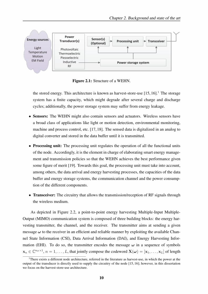
The basic components of a WEHN, which is depicted in Figure 2.1, are:
• Power transducer(s): Different types of energy might be present in the surroundings of
a WEHN (e.g., light, temperature or wind energy); the power transducer is the element in
charge of converting these energy sources into usable electric power. Each energy source
has associated a specific transducer and a wireless node can be equipped with different
transducers, as it is later presented in §2.1.1.
• Power storage system: The electric energy at the output of the transducer is stored in
the power storage system, typically a rechargeable battery, a supercapacitor, a solid state
battery or hybrid solutions. Then, the different circuits of the node are powered with
9
Chapter 2. Background and state of the art
TransceiverProcessing unit
Power storage system
Power
Transducer(s)
Photovoltaic
Thermoelectric
Piezoelectric
Inductive
RF
Sensor(s)
(Optional)Energy sources
Light
Temperature
Motion
EM Field
Figure 2.1: Structure of a WEHN.
the stored energy. This architecture is known as harvest-store-use [15, 16].1 The storage
system has a finite capacity, which might degrade after several charge and discharge
cycles; additionally, the power storage system may suffer from energy leakage.
• Sensors: The WEHN might also contain sensors and actuators. Wireless sensors have
a broad class of applications like light or motion detection, environmental monitoring,
machine and process control, etc. [17, 18]. The sensed data is digitalized in an analog to
digital converter and stored in the data buffer until it is transmitted.
• Processing unit: The processing unit regulates the operation of all the functional units
of the node. Accordingly, it is the element in charge of elaborating smart energy manage-
ment and transmission policies so that the WEHN achieves the best performance given
some figure of merit [19]. Towards this goal, the processing unit must take into account,
among others, the data arrival and energy harvesting processes, the capacities of the data
buffer and energy storage systems, the communication channel and the power consump-
tion of the different components.
• Transceiver: The circuitry that allows the transmission/reception of RF signals through
the wireless medium.
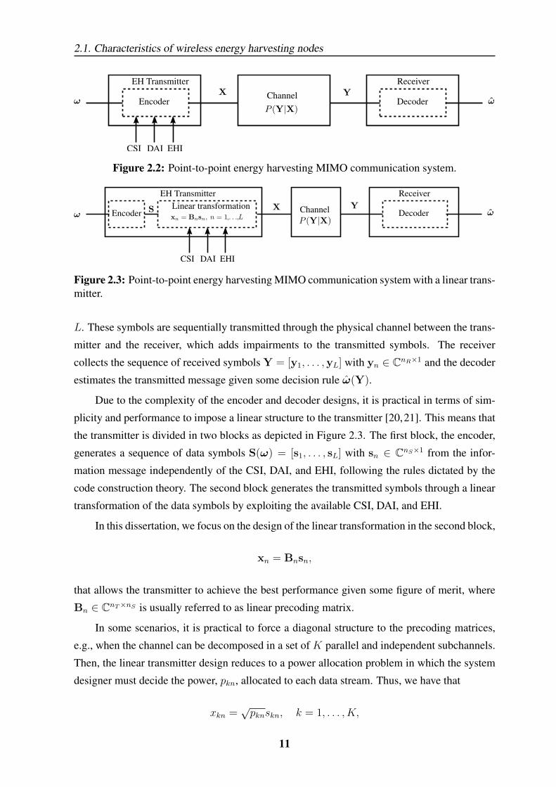
As depicted in Figure 2.2, a point-to-point energy harvesting Multiple-Input Multiple-
Output (MIMO) communication system is composed of three building blocks: the energy har-
vesting transmitter, the channel, and the receiver. The transmitter aims at sending a given
message ω to the receiver in an efficient and reliable manner by exploiting the available Chan-
nel State Information (CSI), Data Arrival Information (DAI), and Energy Harvesting Infor-
mation (EHI). To do so, the transmitter encodes the message ω in a sequence of symbols
xn ∈ CnT×1, n = 1, . . . , L, that jointly compose the codeword X(ω) = [x1, . . . ,xL] of length
1There exists a different node architecture, referred in the literature as harvest-use, in which the power at theoutput of the transducer is directly used to supply the circuitry of the node [15, 16]; however, in this dissertationwe focus on the harvest-store-use architecture.
10
2.1. Characteristics of wireless energy harvesting nodes
Figure 2.2: Point-to-point energy harvesting MIMO communication system.
Figure 2.3: Point-to-point energy harvesting MIMO communication system with a linear trans-mitter.
L. These symbols are sequentially transmitted through the physical channel between the trans-
mitter and the receiver, which adds impairments to the transmitted symbols. The receiver
collects the sequence of received symbols Y = [y1, . . . ,yL] with yn ∈ CnR×1 and the decoder
estimates the transmitted message given some decision rule ω(Y).
Due to the complexity of the encoder and decoder designs, it is practical in terms of sim-
plicity and performance to impose a linear structure to the transmitter [20,21]. This means that
the transmitter is divided in two blocks as depicted in Figure 2.3. The first block, the encoder,
generates a sequence of data symbols S(ω) = [s1, . . . , sL] with sn ∈ CnS×1 from the infor-
mation message independently of the CSI, DAI, and EHI, following the rules dictated by the
code construction theory. The second block generates the transmitted symbols through a linear
transformation of the data symbols by exploiting the available CSI, DAI, and EHI.
In this dissertation, we focus on the design of the linear transformation in the second block,
xn = Bnsn,
that allows the transmitter to achieve the best performance given some figure of merit, where
Bn ∈ CnT×nS is usually referred to as linear precoding matrix.
In some scenarios, it is practical to force a diagonal structure to the precoding matrices,
e.g., when the channel can be decomposed in a set of K parallel and independent subchannels.
Then, the linear transmitter design reduces to a power allocation problem in which the system
designer must decide the power, pkn, allocated to each data stream. Thus, we have that
xkn =√pknskn, k = 1, . . . , K,
11

Chapter 2. Background and state of the art
where K = nT = nR is the total number of independent data streams. In the following lines
of this chapter, we often refer to linear precoding designs; however, the reader must recall
that a power allocation problem is a particular case of a linear precoding design in which the
precoding matrix is forced to have a diagonal structure.
One of the key challenges when dealing with the design of transmission strategies for
WEHNs is that one must account for the temporal variations of the energy availability so that
the node can operate with the best possible performance, which is not easy due to the random
nature of the energy harvesting process. Among others, the following factors must be accounted
for when designing transmission strategies for WEHN:
• Available energy sources and power harvesting profile of the node.
• The communication channel.
• Offline or online transmission strategies, which as explained later refer to the available
knowledge of the CSI, DAI, and EHI.
• Sources of power consumption of the node.
• Chosen figure of merit and constraints.
These factors are thoroughly examined in the following subsections.
2.1.1 Energy sources and power harvesting profile
As presented in Figure 2.1, different types of energy can be present in the surroundings of wire-
less nodes, which can be harvested and transformed to electric power by using the appropriate
conversion technologies. The characteristics of the available energy sources certainly affect
the transmission strategy design. For example, an energy source can be either controllable or
non-controllable; and non-controllable energy sources can be further sorted in predictable or
unpredictable.
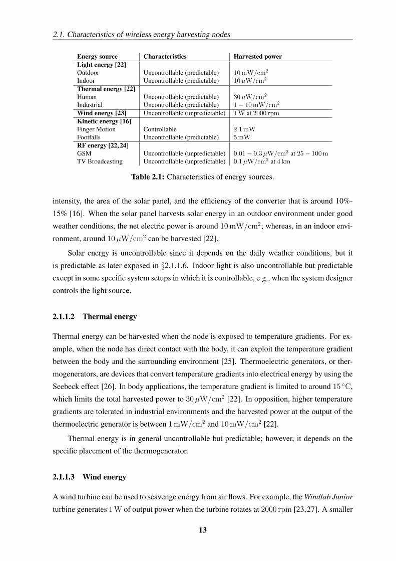
In the following lines, the characteristics of the different energy sources and the associated
transducers are presented, which are summarized in Table 2.1.
2.1.1.1 Light energy
The most commonly exploited source of energy is light energy such as solar radiation or artifi-
cial light. The energy transducer is a solar panel, which is able to generate electricity through
the photovoltaic effect; the amount of generated current is directly proportional to the light
12
2.1. Characteristics of wireless energy harvesting nodes
Energy source Characteristics Harvested powerLight energy [22]Outdoor Uncontrollable (predictable) 10 mW/cm2
Indoor Uncontrollable (predictable) 10µW/cm2
Thermal energy [22]Human Uncontrollable (predictable) 30µW/cm2
Industrial Uncontrollable (predictable) 1− 10 mW/cm2
Wind energy [23] Uncontrollable (unpredictable) 1 W at 2000 rpmKinetic energy [16]Finger Motion Controllable 2.1 mWFootfalls Uncontrollable (predictable) 5 mWRF energy [22, 24]GSM Uncontrollable (unpredictable) 0.01− 0.3µW/cm2 at 25− 100 mTV Broadcasting Uncontrollable (unpredictable) 0.1µW/cm2 at 4 km
Table 2.1: Characteristics of energy sources.
intensity, the area of the solar panel, and the efficiency of the converter that is around 10%-
15% [16]. When the solar panel harvests solar energy in an outdoor environment under good
weather conditions, the net electric power is around 10 mW/cm2; whereas, in an indoor envi-
ronment, around 10µW/cm2 can be harvested [22].
Solar energy is uncontrollable since it depends on the daily weather conditions, but it
is predictable as later exposed in §2.1.1.6. Indoor light is also uncontrollable but predictable
except in some specific system setups in which it is controllable, e.g., when the system designer
controls the light source.
2.1.1.2 Thermal energy
Thermal energy can be harvested when the node is exposed to temperature gradients. For ex-
ample, when the node has direct contact with the body, it can exploit the temperature gradient
between the body and the surrounding environment [25]. Thermoelectric generators, or ther-
mogenerators, are devices that convert temperature gradients into electrical energy by using the
Seebeck effect [26]. In body applications, the temperature gradient is limited to around 15 ◦C,
which limits the total harvested power to 30µW/cm2 [22]. In opposition, higher temperature
gradients are tolerated in industrial environments and the harvested power at the output of the
thermoelectric generator is between 1 mW/cm2 and 10 mW/cm2 [22].
Thermal energy is in general uncontrollable but predictable; however, it depends on the
specific placement of the thermogenerator.
2.1.1.3 Wind energy
A wind turbine can be used to scavenge energy from air flows. For example, the Windlab Junior
turbine generates 1 W of output power when the turbine rotates at 2000 rpm [23,27]. A smaller
13

Chapter 2. Background and state of the art
Figure 2.4: Wind turbine implemented in a wireless sensor node in [28].
wind turbine that provides an output power in the range of 7.3 − 55 mW was used in [28] to
power the wireless sensor node depicted in Figure 2.4.
Wind energy is in general an uncontrollable and unpredictable energy source as fast vari-
ations in the air flow can easily occur. Nevertheless, if the airflow is generated by industrial
applications, the harvested energy might be predictable or even controllable.
2.1.1.4 Kinetic energy
Vibrations are commonly encountered in bridges, roads, commercial buildings, automobiles,
etc. Accordingly, movements or vibrations of objects are another potential source of energy for
wireless nodes. The most common transducers to harvest vibrational energy are piezoelectric
generators or electrostatic and electromagnetic converters [29–31].
The available energy might be due to uncontrollable environmental vibrations, human
active or human passive. Human active sources require the user to perform a specific power
generating motion and are generally controllable; for example, finger motion is able to produce
an output power of 2.1 mW [16]. In opposition, human passive energy refers to the energy
generated by humans in habitual gestures and movements, e.g., the heel impact in the floor
while walking generates an output power of 5 mW, which might be predictable [16].
14
2.1. Characteristics of wireless energy harvesting nodes
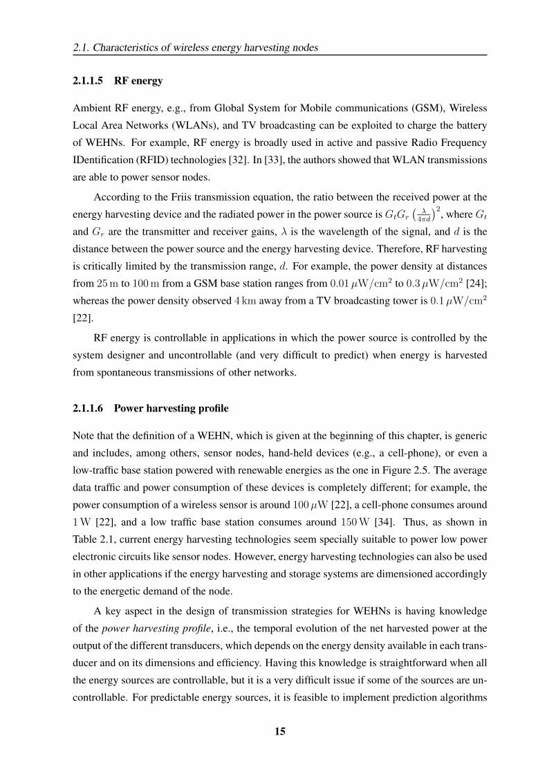
2.1.1.5 RF energy
Ambient RF energy, e.g., from Global System for Mobile communications (GSM), Wireless
Local Area Networks (WLANs), and TV broadcasting can be exploited to charge the battery
of WEHNs. For example, RF energy is broadly used in active and passive Radio Frequency
IDentification (RFID) technologies [32]. In [33], the authors showed that WLAN transmissions
are able to power sensor nodes.
According to the Friis transmission equation, the ratio between the received power at the
energy harvesting device and the radiated power in the power source is GtGr
(λ
4πd
)2, where Gt
and Gr are the transmitter and receiver gains, λ is the wavelength of the signal, and d is the
distance between the power source and the energy harvesting device. Therefore, RF harvesting
is critically limited by the transmission range, d. For example, the power density at distances
from 25 m to 100 m from a GSM base station ranges from 0.01µW/cm2 to 0.3µW/cm2 [24];
whereas the power density observed 4 km away from a TV broadcasting tower is 0.1µW/cm2
[22].
RF energy is controllable in applications in which the power source is controlled by the
system designer and uncontrollable (and very difficult to predict) when energy is harvested
from spontaneous transmissions of other networks.
2.1.1.6 Power harvesting profile
Note that the definition of a WEHN, which is given at the beginning of this chapter, is generic
and includes, among others, sensor nodes, hand-held devices (e.g., a cell-phone), or even a
low-traffic base station powered with renewable energies as the one in Figure 2.5. The average
data traffic and power consumption of these devices is completely different; for example, the
power consumption of a wireless sensor is around 100µW [22], a cell-phone consumes around
1 W [22], and a low traffic base station consumes around 150 W [34]. Thus, as shown in
Table 2.1, current energy harvesting technologies seem specially suitable to power low power
electronic circuits like sensor nodes. However, energy harvesting technologies can also be used
in other applications if the energy harvesting and storage systems are dimensioned accordingly
to the energetic demand of the node.
A key aspect in the design of transmission strategies for WEHNs is having knowledge
of the power harvesting profile, i.e., the temporal evolution of the net harvested power at the
output of the different transducers, which depends on the energy density available in each trans-
ducer and on its dimensions and efficiency. Having this knowledge is straightforward when all
the energy sources are controllable, but it is a very difficult issue if some of the sources are un-
controllable. For predictable energy sources, it is feasible to implement prediction algorithms
15
Chapter 2. Background and state of the art
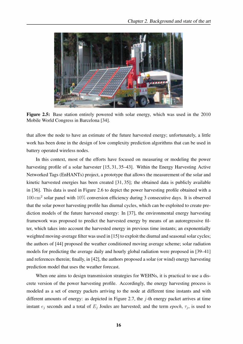
Figure 2.5: Base station entirely powered with solar energy, which was used in the 2010Mobile World Congress in Barcelona [34].
that allow the node to have an estimate of the future harvested energy; unfortunately, a little
work has been done in the design of low complexity prediction algorithms that can be used in
battery operated wireless nodes.
In this context, most of the efforts have focused on measuring or modeling the power
harvesting profile of a solar harvester [15, 31, 35–43]. Within the Energy Harvesting Active
Networked Tags (EnHANTs) project, a prototype that allows the measurement of the solar and
kinetic harvested energies has been created [31, 35]; the obtained data is publicly available
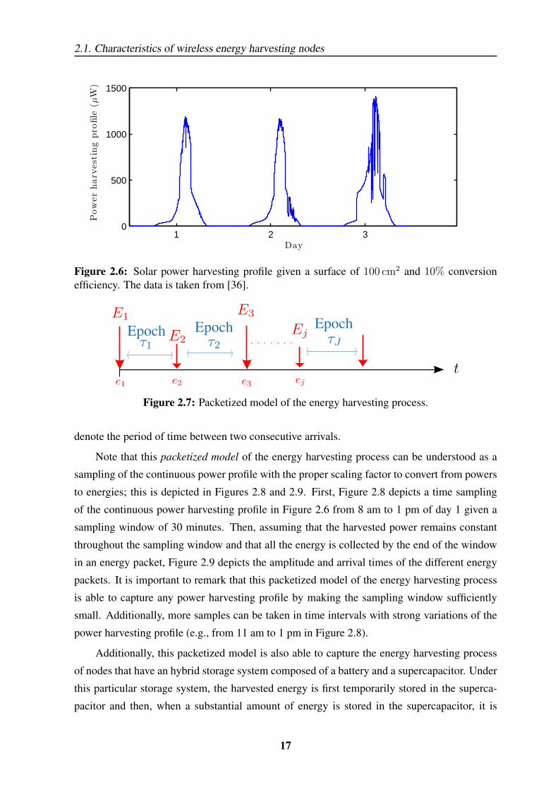
in [36]. This data is used in Figure 2.6 to depict the power harvesting profile obtained with a
100 cm2 solar panel with 10% conversion efficiency during 3 consecutive days. It is observed
that the solar power harvesting profile has diurnal cycles, which can be exploited to create pre-
diction models of the future harvested energy: In [37], the environmental energy harvesting
framework was proposed to predict the harvested energy by means of an autoregressive fil-
ter, which takes into account the harvested energy in previous time instants; an exponentially
weighted moving-average filter was used in [15] to exploit the diurnal and seasonal solar cycles;
the authors of [44] proposed the weather conditioned moving average scheme; solar radiation
models for predicting the average daily and hourly global radiation were proposed in [39–41]
and references therein; finally, in [42], the authors proposed a solar (or wind) energy harvesting
prediction model that uses the weather forecast.
When one aims to design transmission strategies for WEHNs, it is practical to use a dis-
crete version of the power harvesting profile. Accordingly, the energy harvesting process is
modeled as a set of energy packets arriving to the node at different time instants and with
different amounts of energy: as depicted in Figure 2.7, the j-th energy packet arrives at time
instant ej seconds and a total of Ej Joules are harvested; and the term epoch, τj , is used to
16
2.1. Characteristics of wireless energy harvesting nodes
1 2 30
500
1000
1500Powerharv
estingpro
file
(µW
)
Day
Figure 2.6: Solar power harvesting profile given a surface of 100 cm2 and 10% conversionefficiency. The data is taken from [36].
Figure 2.7: Packetized model of the energy harvesting process.
denote the period of time between two consecutive arrivals.
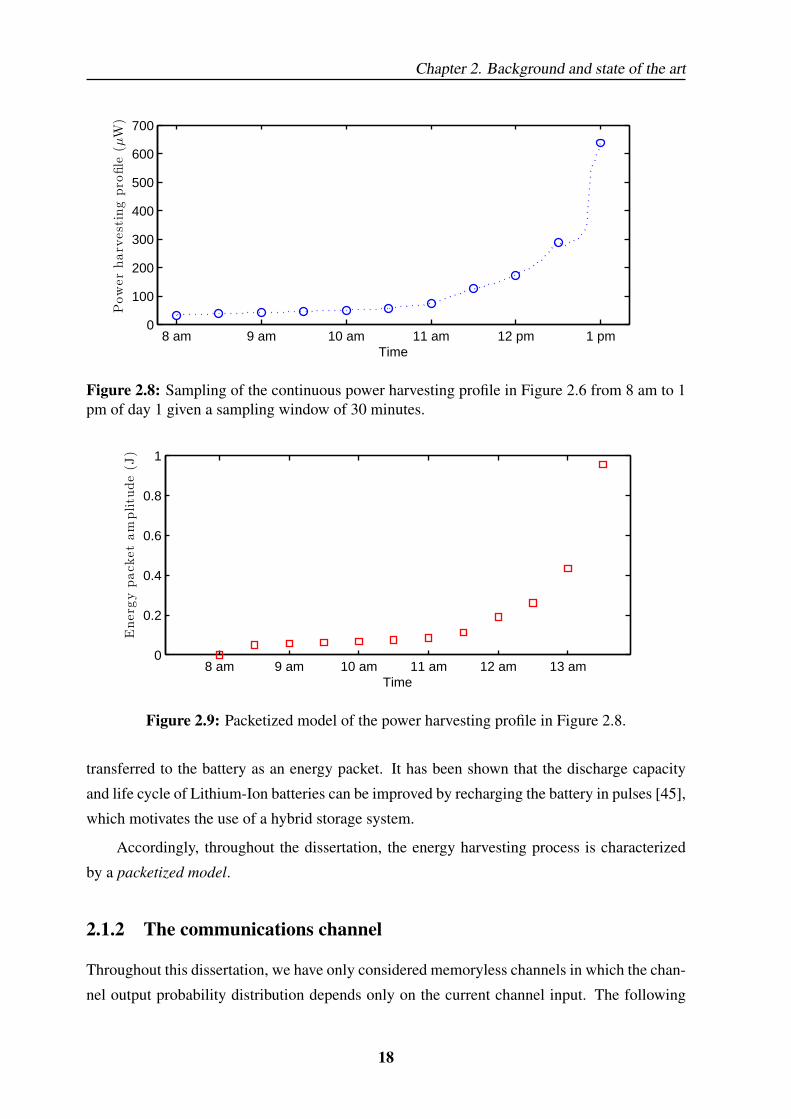
Note that this packetized model of the energy harvesting process can be understood as a
sampling of the continuous power profile with the proper scaling factor to convert from powers
to energies; this is depicted in Figures 2.8 and 2.9. First, Figure 2.8 depicts a time sampling
of the continuous power harvesting profile in Figure 2.6 from 8 am to 1 pm of day 1 given a
sampling window of 30 minutes. Then, assuming that the harvested power remains constant
throughout the sampling window and that all the energy is collected by the end of the window
in an energy packet, Figure 2.9 depicts the amplitude and arrival times of the different energy
packets. It is important to remark that this packetized model of the energy harvesting process
is able to capture any power harvesting profile by making the sampling window sufficiently
small. Additionally, more samples can be taken in time intervals with strong variations of the
power harvesting profile (e.g., from 11 am to 1 pm in Figure 2.8).
Additionally, this packetized model is also able to capture the energy harvesting process
of nodes that have an hybrid storage system composed of a battery and a supercapacitor. Under
this particular storage system, the harvested energy is first temporarily stored in the superca-
pacitor and then, when a substantial amount of energy is stored in the supercapacitor, it is
17
Chapter 2. Background and state of the art
8 am 9 am 10 am 11 am 12 pm 1 pm0
100
200
300
400
500
600
700Powerharv
estingpro
file
(µW
)
Time
Figure 2.8: Sampling of the continuous power harvesting profile in Figure 2.6 from 8 am to 1pm of day 1 given a sampling window of 30 minutes.
8 am 9 am 10 am 11 am 12 am 13 am0
0.2
0.4
0.6
0.8
1
Energ
ypack
etamplitu
de(J
)
Time
Figure 2.9: Packetized model of the power harvesting profile in Figure 2.8.
transferred to the battery as an energy packet. It has been shown that the discharge capacity
and life cycle of Lithium-Ion batteries can be improved by recharging the battery in pulses [45],
which motivates the use of a hybrid storage system.
Accordingly, throughout the dissertation, the energy harvesting process is characterized
by a packetized model.
2.1.2 The communications channel
Throughout this dissertation, we have only considered memoryless channels in which the chan-
nel output probability distribution depends only on the current channel input. The following
18
2.1. Characteristics of wireless energy harvesting nodes
lines present the channel models that are relevant to the following chapters.
2.1.2.1 The linear vector Gaussian channel
A linear vector Gaussian channel is such that the output of the channel, y ∈ CnR×1, is a linear
function of the input, x ∈ CnT×1, i.e.,
y = Gx + w, (2.1)
where G ∈ CnR×nT is the channel matrix and w ∈ CnR×1 is a circularly symmetric com-
plex Gaussian random variable with zero mean and covariance matrix given by Rw, w ∼CN (0,Rw), that models the thermal noise and other undesired effects in the receiving RF
front-ends.
Many practical communication systems of interest can be modeled as a linear vector Gaus-
sian channel. For example, in a multi-antenna wireless channel, nT and nR denote the number
of antennas at the transmitter and receiver, respectively, and the element in the r-th row and
t-th column of G denotes the channel coefficient between the t-th antenna at the transmitter
and r-th antenna at the receiver. Other examples of systems that can be modeled as (2.1) are:
Digital Subscriber Line (DSL); Code Division Multiple Access (CDMA); multicarrier systems
like Orthogonal Frequency Division Multiplexing (OFDM) or Discrete Multi-Tone (DMT);
etc. [20].
2.1.2.2 Parallel transmissions over Gaussian scalar channels
A particular case of special interest throughout the dissertation occurs when the channel matrix
is diagonal, i.e., G = Diag([g1, . . . , gK ]T), since then the system model can be rewritten as a
set of K parallel scalar channels:
yk = gkxk + wk, k = 1, . . . , K. (2.2)
2.1.2.3 Interfering multiuser communications
In practice, it is common to encounter scenarios where several transmitter and receiver pairs
must share the same channel. When this happens, the transmission of the different users gener-
ally interfere each other, which must be accounted for in the design of the transmission strategy
of each user.
In Chapter 6, we consider a Gaussian interference channel composed of T transmitter
and receiver pairs sharing the same band over SISO frequency-selective links composed of K
19

Chapter 2. Background and state of the art
parallel subcarriers. In this setup, the received signal at the t-th receiver and k-th subchannel is
yt(k) = gtt(k)xt(k) + wt(k)︸ ︷︷ ︸Noise
+∑t′ 6=t
gt′t(k)xt′(k)︸ ︷︷ ︸MUI
, (2.3)
where gtr(k) is the channel value between the t-th transmitter and the r-th receiver at the k-th
subcarrier; xt(k) is the transmitted symbol by user t at the k-th subcarrier; wt(k) denotes the
noise at the t-th receiver and k-th subcarrier; and the term∑
t′ 6=t gt′t(k)xt′(k) is the MultiUser
Interference (MUI) at the t-th receiver and k-th subcarrier.
Note that, in practical communication systems, several independent channel accesses are
produced over time. Throughout this dissertation, we denote the temporal accesses with the
index n. Accordingly, we will further index the expressions in (2.1), (2.2), and (2.3) by n.
2.1.3 Offline and online transmission strategies
There exist two well established approaches for the design of transmission strategies, which
apply to both WEHNs and classical non-harvesting nodes, namely, online and offline. These
approaches differ on the available knowledge at the transmitter of random parameters that
influence transmission, e.g., CSI, DAI, and EHI.
In offline transmission strategies, the transmitter node has full knowledge (i.e., from the
past, present, and future realizations) of these random parameters.
In opposition, online transmission strategies consider that the transmitter only has causal
knowledge (i.e., from the past and present realizations) of these random parameters and maybe
some statistical information regarding its future behaviour.
The study of offline transmission strategies is of key importance due to the following
reasons.
(1.) The offline transmission strategy can be found independently of the specific choice of
energy transducers in the node since, as introduced in §2.1.1.6, the packetized model of
the energy harvesting process applies to any power harvesting profile. In opposition, on-
line transmission strategies must account for the power harvesting profiles and statistical
information of each specific energy source.
(2.) In some scenarios, it is indeed feasible to have full knowledge of these random parame-
ters. For example, when the channel is time-static, the transmitter knows the arrival time
of the data packets (e.g., a sensor that takes periodic measurements or when there is a
sufficiently long backlog of data to be transmitted), and the energy source is controllable
20
2.1. Characteristics of wireless energy harvesting nodes
or uncontrollable but predictable in the time window in which the transmission scheme is
being designed (e.g., the solar power harvesting profile can be predicted with the models
introduced in §2.1.1.6).
In other scenarios, where indeed the transmitter only has causal knowledge of these random
parameters:
(3.) The optimal offline transmission strategy gives a bound on the achievable performance
by any online strategy:
• When the transmitter is designed to maximize some utility function, then the opti-
mal offline transmission strategy gives an upper bound on the achievable utility.
• In opposition, when the design objective is the minimization of a cost function, then
the optimal offline transmission strategy gives a lower bound on the achievable cost.
(4.) In many cases, it provides analytical and intuitive solutions, which can be later used for
the design of online transmission strategies.
Therefore, the derivation of the offline transmission strategy is a good first step to gain
insight for the later design of the online transmission strategies.
2.1.4 Sources of power consumption
Traditional transmission strategies consider that the radiated power is the unique source of
energy consumption at the transmitter (as it is later presented in §2.2). This is a reasonable as-
sumption when the transmission power is large, which occurs in long-range communications,
since it dominates over other sinks of energy. However, in certain applications, the trans-
mission power might be comparable to the remaining energy sinks. For example, in energy
efficient network topologies, transmission distances may be below 10 m and the circuitry en-
ergy consumption caused by the different components of the RF chain becomes relevant, even
dominating over the radiated power [46, 47]. This often occurs to low-consumption devices
such as sensor nodes that are powered by energy harvesting.
A more realistic power consumption model is given in [47–51], where the total consumed
power is modeled as2
C1(p) =
ξ
ηp+ α if p > 0,
δ if p = 0,
(2.4)
2Different power consumption models are used through the dissertation. Accordingly, the i-th power con-sumption model is denoted as Ci.
21

Chapter 2. Background and state of the art
where p denotes the transmission radiated power; α accounts for both the power consumption
of the digital to analog converter and for the consumption of the different components of the
radio frequency chain, which includes the mixer, the filters, and the synthesizer; ξ and η are
the power amplifier output back-off and drain efficiency, respectively [48]; and δ models the
circuitry consumption when the transmitter is silent, which is much smaller than α.
For convenience, we introduce the following equivalent formulation of (2.4):
C1(p) =ξ
ηp+ (α− δ)H` (p) + δ, (2.5)
whereH` (x) is the left continuous unit step function defined as
H` (x) =
1 if x > 0,
0 if x ≤ 0.(2.6)
This model is able to capture the consumption of having the node “on”, but it is still a
clear simplification from reality because, among others, it ignores the power consumption of
transitions between the “off” and “on” states, which are associated to the startup time of the
transmitter [51].
As it is later presented in §2.2.1.3 and Chapters 5 and 6, the discontinuity of C1 at the
origin substantially complicates the design of transmission strategies with respect to (w.r.t.)
solely considering the transmission radiated power.
2.1.5 Figure of merit and constraints
There are several figures of merit or objective functions that can be investigated when designing
transmission strategies. Some examples that have been considered in the literature are:
(1.) Minimization of the Mean-Square Error (MSE) [52, 53].
(2.) Minimization of the Bit Error Rate (BER) [53].
(3.) Minimization of the total energy consumption to transmit a certain amount of information
by a given deadline [54, 55].
(4.) Maximization of the mean Signal to Interference plus Noise Ratio (SINR) [53].
(5.) Maximization of the mutual information [56–59].
(6.) Minimization of the total transmission time of a certain amount of information [60].
22

2.1. Characteristics of wireless energy harvesting nodes
In this dissertation, we focus on the figures of merit 5 and 6 leaving the remaining ones as
possible future research directions.
Given any figure of merit, the system performance is, in practice, limited by the available
resources (e.g., a finite amount of energy, bandwidth, transmission time, etc.) or by some
specific design requirements (e.g., a minimum Signal to Noise Ratio (SNR) at the receiver, a
maximum delay constraint, etc.).
In the following lines, we summarize the common limitations that appear when designing
transmission strategies for WEHNs.
• Energy Causality Constraints (ECCs): As it has been briefly introduced in the previous
chapter, the presence of energy harvesters implies a loss of optimality of the traditional
transmission policies for non-harvesting nodes because the ECCs must be taken into ac-
count, which impose that the energy cumulatively used by the node at a certain time
instant must be no greater than the energy cumulatively harvested and stored on the bat-
tery. Accordingly, the ECCs mainly depend on the battery capacity (since energy lost due
to battery overflows cannot be later used), the packetized model of the energy harvesting
process (cf. §2.1.1.6), and the considered power consumption model (cf. §2.1.4). Other
factors such as battery capacity degradation or leakages can also be considered in the
ECCs (see , e.g., [61, 62]); however, this dissertation considers an ideal storage system.
The ECCs can be imposed instantaneously or by averaging over the transmitted symbols;
nevertheless, most of the works in the literature consider the averaged ECCs since it is
commonly assumed that the dynamics of the energy harvesting process are much slower
than the symbol duration.
• Instantaneous mask constraints: The temporal and/or spectral mask constraints limit
the maximum transmitted power at a certain time instant and/or over a certain subcar-
rier. These constraints are generally imposed either by radio regulatory bodies or by the
maximum output power at the power amplifier.
• Data Causality Constraints (DCCs): This set of constraints applies when the data to
be transmitted is collected dynamically over time, which occurs, for instance, when the
node takes periodic measurements of some event(s) through the sensor(s). Similarly to
the ECCs above, the DCCs impose that the data cumulatively transmitted by the node at
a certain time instant must be no greater than the data that have cumulatively arrived to
the data buffer.
• Finite data buffer constraint: This constraint applies when the buffer to store the data
to be transmitted is finite and imposes that no data is lost due to buffer overflows.
23

Chapter 2. Background and state of the art
• QoS constraints: QoS constraints impose a given performance on the quality of the
received message. For example, it might be convenient to bound the maximum transmis-
sion delay, the maximum probability of error or the minimum SNR.
2.1.6 Linear transmitter design problem formulation
The linear transmitter design problem can be, in general, mathematically formulated as the
following optimization problem
minimize{Bn}Nn=1
f({Bn}Nn=1
)(2.7a)
subject to gi({Bn}Nn=1
)≤ 0, i = 1, . . . ,m, (2.7b)
where N denotes the number of channel accesses in which the transmitter is being designed;
{Bn}Nn=1 is the set of precoding matrices from the channel access 1 to N , which are the opti-
mization variables; f is the objective function; and the functions gi denote a set of m inequality
constraints. These functions depend on all the factors presented above (packetized model of the
energy harvesting process, channel model, offline or online implementation, sources of power
consumption, figure of merit, practical design constraints, etc.).
Note that for compactness we have formulated the transmitter design problem as a discrete-
time linear precoding design; however, without loss of generality, it can also be formulated as
a time continuous problem or as a power allocation problem (when the precoding matrix is
forced to have a diagonal structure). In the remaining chapters of the dissertation, we deal both
with continuous and discrete-time designs.
Convex optimization theory3 dictates that if the functions f and gi are convex, then the
optimization problem in (2.7) is a convex program (or convex optimization problem) whose
optimal solution can be found by standard convex optimization techniques [63].
Unfortunately, in many transmitter designs of interest, e.g., the problems explored in Chap-
ters 3-6, the optimization problem in (2.7) is nonconvex and, accordingly, determining its so-
lution is more involved.
Depending on the structure of the problem, one may still be able to derive a globally
optimal solution to the nonconvex problem. For example, in some problems of interest, it is
possible to reformulate the problem as an equivalent convex optimization problem that can be
solved by convex optimization theory, e.g., by doing a change of variables. However, such a
reformulation does not always exist; in these situations, a common approach in the literature
3The following chapters of this dissertation make use of convex optimization theory, which is not introducedhere since it is currently well-known in the information and communication theory community; the interestedreader is referred to [63].
24
2.2. State of the art on transmission strategiesfor non-harvesting nodes
is to relax some of the constraints to obtain a more tractable problem or to simply accept a
feasible solution that performs close to the optimal one.
There exist several nonconvex optimization algorithms in the literature (e.g., gradient-
based descend schemes [64], Successive Convex Approximation (SCA) algorithms [65–67],
feasible sequential quadratic programming [68], parallel variable distribution [69], etc.), which
are iterative and guarantee converge to some locally optimal solution.
When the constraints are convex, but the objective function is nonconvex, a common ap-
proach is to use gradient-based descend schemes, e.g., the Frank-Wolfe method [64], which
linearizes the objective function around the current iterate and solves the resulting convex pro-
gram to find the updated direction. In opposition, the algorithm in [66], which is based on
SCA, convexifies only the nonconvex part of the objective function, thus exploiting any possi-
ble degree of convexity in the objective function, which results in a faster convergence speed.
The algorithm in [67] generalizes the work in [66] to deal also with nonconvex constraints.
Throughout this dissertation, we explore different alternatives to deal with nonconvex
transmitter design problems.
The following section presents the relevant state of the art of known transmission strategies
for non-harvesting nodes.
2.2 State of the art on transmission strategies
for non-harvesting nodes
2.2.1 Maximization of the mutual information
Channel capacity was originally derived by Shannon for single-user time invariant channels
as the maximum mutual information between the channel input and output. Equivalently, the
channel capacity is the maximum data transmission rate such that the probability of error can
be made arbitrarily small by using a sufficiently long transmission block [70].
When the channel is time-varying, several definitions of channel capacity apply depending
on the available CSI, e.g., the instantaneous capacity, the ergodic capacity or outage capacity
(see the tutorial in [71] for more details). This dissertation considers the idealistic situation in
which both the transmitter and receiver know perfectly and instantaneously the channel matrix,
which happens when the channel is static or when the channel coherence time is much larger
than the symbol duration so that it is constant for a sufficient number of transmissions. In such
scenario, the channel can be considered as time invariant.
25
Chapter 2. Background and state of the art
2.2.1.1 Classical Water-Filling (CWF)
The instantaneous capacity of the linear vector Gaussian channel in (2.1), i.e., y = Gx + w, is
obtained by using a Gaussian code with transmission covariance matrix Q, x ∼ CN (0,Q), as
maximizeQ
I(x; y) (2.8a)
subject to Tr(Q) ≤ P , (2.8b)
where I(x; y) , log det(InR + R−1w GQGH) is the mutual information [56] and the constraint
in (2.8b) imposes a limitation on the average transmit power.
As shown by Telatar in [56], capacity can be achieved by diagonalizing the whitened
channel matrix, which has the following Gram matrix RG = GHR−1w G that can be equivalently
written in terms of its eigenvalue decomposition as RG = URGDRGUHRG
, where URG contains
the eigenvectors of RG and DRG contains the associated eigenvalues hk, k = 1, . . . , K, i.e.,
DRG = Diag([h1, . . . , hK ]T), where K = nT . Accordingly, the channel is diagonalized when
the transmit covariance matrix has the following structure
Q = URGDQUHRG,
where DQ = Diag([p1, . . . , pK ]T).
As a result of diagonalizing the channel, the original linear vector channel is equivalent to
a set of K parallel scalar channels whose capacity is obtained by solving the following power
allocation problem:
maximize{pk}Kk=1
K∑k=1
log(1 + hkpk) (2.9a)
subject toK∑k=1
pk ≤ P , (2.9b)
where it has been used that the capacity of a scalar Additive White Gaussian Noise (AWGN)
channel is log(1 + hkpk) [72]. Since the objective function is concave and the constraint
is affine, (2.9) is a convex optimization problem and can be easily solved by means of the
Karush–Kuhn–Tucker (KKT) optimality conditions [63] from where the CWF power alloca-
tion is obtained as
p?k =
[W − 1
hk
]+
, (2.10)
where hk is the channel gain of the k-th parallel stream andW is the water level that is obtained
by imposing that the power constraint must be satisfied with equality,∑K
k=1 p?k = P .
26

2.2. State of the art on transmission strategiesfor non-harvesting nodes
Figure 2.10: Graphical representation of CWF. In this specific representation, no power isassigned to the subchannels 4, 5, and 6.
The CWF solution accepts an intuitive graphical representation that is depicted in Figure
2.10 and proceeds as follows:
(1.) Each parallel channel is represented with a unit-base water-porous vessel.
(2.) Each vessel is filled with a solid substance up to a height equal to h−1k .
(3.) A volume of water equal to P is poured through the vessels.
(4.) Finally, the optimal power allocation in each parallel channel is the height of water in
each vessel.
From the graphical representation, it is clear that higher power is assigned to the parallel chan-
nels (or eigenmodes) with higher channel gains. Additionally, zero power is assigned to those
subchannels in which the water level does not reach the height 1hk
.
2.2.1.2 Mercury/Water-Filling (HgWF)
To derive the CWF solution in (2.10), the distribution of the input symbols is chosen to be
Gaussian because it is the one that provides the highest mutual information [72]. Unfortunately,
current technology cannot cope with Gaussian codes and finite constellations are used instead,
e.g.,M-PAM andM-QAM, whereM denotes the alphabet cardinality.
In the low SNR regime, the capacity achieved with finite constellations is very close to
the one achieved with Gaussian signaling. However, the mutual information asymptotically
saturates when the SNR increases as no more than log2M bit per channel use can be sent (see
Figure 1 in [73]). Accordingly, in practical setups, the CWF solution in (2.10) is a theoretical
limit that might be far from the real one [73].
27
Chapter 2. Background and state of the art
This must be taken into account in the design of the optimal power allocation when the
input symbols are constrained to belong to a finite alphabet. In opposition to the Gaussian case,
where the better the channel gain, the higher the allocated power, when arbitrary constellations
are used, the relation between the allocated power and the channel gain depends on the alphabet
cardinality.
In [57], the authors derived the power allocation that maximizes the mutual information
of a set of parallel channels, when the distribution of the input symbols is fixed and given. To
do so, the authors of [57] used the relation between the mutual information and the Minimum
Mean-Square Error (MMSE), which was revealed in [74] and further generalized in [75], as
summarized in the following lines.
In [74], Guo et al. revealed that the derivative of the mutual information w.r.t. the SNR for
a real-valued scalar Gaussian channel is proportional to the MMSE, i.e.,
ddhI(x;√hx+ w) =
1
2mmse(h), (2.11)
where x is the channel input, w is the observed noise with w ∼ N (0, 1) and mmse(h) =
E {(x− x)2}, where x = E {x|√hx+ w} is the conditional mean estimator.
The mutual information in linear vector Gaussian channels was further characterized in
[75], where its partial derivatives w.r.t. arbitrary system parameters were determined, e.g., the
gradient w.r.t. the channel matrix, G, was found to be
∇GI(x; Gx + w) = GE, (2.12)
where E = E {(x− x)(x− x)H} is the MMSE matrix, and x = E {x|Gx + w}.
Thanks to the relationship in (2.11), the power allocation that maximizes the mutual infor-
mation over a set of parallel channels (each of them denoted by a different index k) with finite
alphabet inputs was derived in [57] and named Mercury/Water-Filling (HgWF), i.e.,
p?k =
[W − 1
hkGk
(1
Whk
)]+
, (2.13)
where Gk(ψ) is the mercury factor that depends on the input distribution and is defined as
Gk(ψ) =
1ψ−mmse−1
k (ψ) if ψ ∈ [0, 1],
1 if ψ ≥ 1,(2.14)
and mmse−1k (ψ) is the inverse MMSE function, which returns the required SNR to achieve a
certain MMSE ψ and depends on the input distribution. This result showed that the optimal
28

2.2. State of the art on transmission strategiesfor non-harvesting nodes
power allocation not only depends on the channel gain as in the Gaussian signaling case but
also on the shape and size of the input constellation.
In particular, when the input symbols are drawn from a Gaussian distribution, x ∼ N (0, 1),
then the MMSE function and the inverse MMSE function are
mmse(h) =1
1 + h(2.15)
and
mmse−1(ψ) =1− ψψ
, (2.16)
respectively. With this, it follows that Gk(ψ) = 1,∀ψ, from where it is easy to check that the
CWF solution in (2.10) is recovered after particularizing the HgWF in (2.13) for a Gaussian
input distribution.
Interestingly, the HgWF solution also accepts a graphical representation that is depicted
in Figure 2.11 and summarized in the following lines:
(1.) Each parallel channel is represented with a unit-base water-porous mercury-nonporous
vessel.
(2.) Then, each vessel is filled with a solid substance up to a height equal to h−1k .
(3.) Given the optimal water level W , pour mercury in each vessel until the mercury level
(i.e., the height of the mercury from the ground level) is 1hkGk
(1
Whk
).
(4.) Pour a volume of water equal to P (note that the resulting water level must be W ).
(5.) Finally, the optimal power allocation in each parallel channel is found as the difference
between the water and mercury levels.
Note that both the CWF (2.10) and theHgWF (2.13) are parametric solutions that depend
on the water level W . In opposition to CWF, where the value of the optimal water level W
is obtained directly from the graphical interpretation, in the HgWF solution the optimal water
level W must be numerically computed in advance for the graphical interpretation to apply.
In Chapter 4, we generalize the HgWF solution to include energy harvesting at the trans-
mitter and propose a graphical interpretation that does not require previous knowledge of the
optimal water level.
It is important to remark that the HgWF presented above only applies when the chan-
nel and linear precoder matrices are diagonal. When general channel and precoder matrices
are considered, finding the precoder that maximizes the mutual information is indeed quite
29
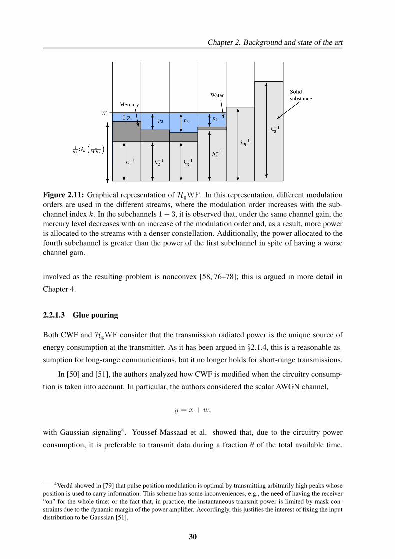
Chapter 2. Background and state of the art
Figure 2.11: Graphical representation of HgWF. In this representation, different modulationorders are used in the different streams, where the modulation order increases with the sub-channel index k. In the subchannels 1− 3, it is observed that, under the same channel gain, themercury level decreases with an increase of the modulation order and, as a result, more poweris allocated to the streams with a denser constellation. Additionally, the power allocated to thefourth subchannel is greater than the power of the first subchannel in spite of having a worsechannel gain.
involved as the resulting problem is nonconvex [58, 76–78]; this is argued in more detail in
Chapter 4.
2.2.1.3 Glue pouring
Both CWF and HgWF consider that the transmission radiated power is the unique source of
energy consumption at the transmitter. As it has been argued in §2.1.4, this is a reasonable as-
sumption for long-range communications, but it no longer holds for short-range transmissions.
In [50] and [51], the authors analyzed how CWF is modified when the circuitry consump-
tion is taken into account. In particular, the authors considered the scalar AWGN channel,
y = x+ w,
with Gaussian signaling4. Youssef-Massaad et al. showed that, due to the circuitry power
consumption, it is preferable to transmit data during a fraction θ of the total available time.
4Verdu showed in [79] that pulse position modulation is optimal by transmitting arbitrarily high peaks whoseposition is used to carry information. This scheme has some inconveniences, e.g., the need of having the receiver“on” for the whole time; or the fact that, in practice, the instantaneous transmit power is limited by mask con-straints due to the dynamic margin of the power amplifier. Accordingly, this justifies the interest of fixing the inputdistribution to be Gaussian [51].
30
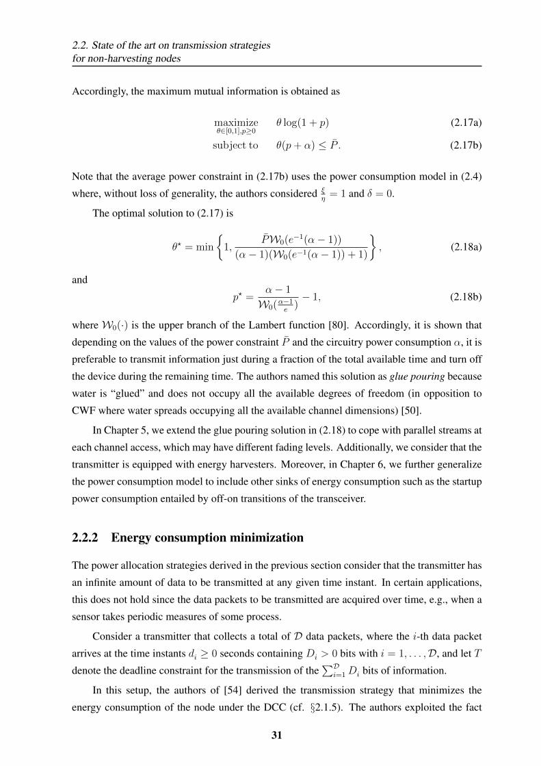
2.2. State of the art on transmission strategiesfor non-harvesting nodes
Accordingly, the maximum mutual information is obtained as
maximizeθ∈[0,1],p≥0
θ log(1 + p) (2.17a)
subject to θ(p+ α) ≤ P . (2.17b)
Note that the average power constraint in (2.17b) uses the power consumption model in (2.4)
where, without loss of generality, the authors considered ξη
= 1 and δ = 0.
The optimal solution to (2.17) is
θ? = min
{1,
PW0(e−1(α− 1))
(α− 1)(W0(e−1(α− 1)) + 1)
}, (2.18a)
and
p? =α− 1
W0(α−1e
)− 1, (2.18b)
where W0(·) is the upper branch of the Lambert function [80]. Accordingly, it is shown that
depending on the values of the power constraint P and the circuitry power consumption α, it is
preferable to transmit information just during a fraction of the total available time and turn off
the device during the remaining time. The authors named this solution as glue pouring because
water is “glued” and does not occupy all the available degrees of freedom (in opposition to
CWF where water spreads occupying all the available channel dimensions) [50].
In Chapter 5, we extend the glue pouring solution in (2.18) to cope with parallel streams at
each channel access, which may have different fading levels. Additionally, we consider that the
transmitter is equipped with energy harvesters. Moreover, in Chapter 6, we further generalize
the power consumption model to include other sinks of energy consumption such as the startup
power consumption entailed by off-on transitions of the transceiver.
2.2.2 Energy consumption minimization
The power allocation strategies derived in the previous section consider that the transmitter has
an infinite amount of data to be transmitted at any given time instant. In certain applications,
this does not hold since the data packets to be transmitted are acquired over time, e.g., when a
sensor takes periodic measures of some process.
Consider a transmitter that collects a total of D data packets, where the i-th data packet
arrives at the time instants di ≥ 0 seconds containing Di > 0 bits with i = 1, . . . ,D, and let T
denote the deadline constraint for the transmission of the∑D
i=1 Di bits of information.
In this setup, the authors of [54] derived the transmission strategy that minimizes the
energy consumption of the node under the DCC (cf. §2.1.5). The authors exploited the fact
31
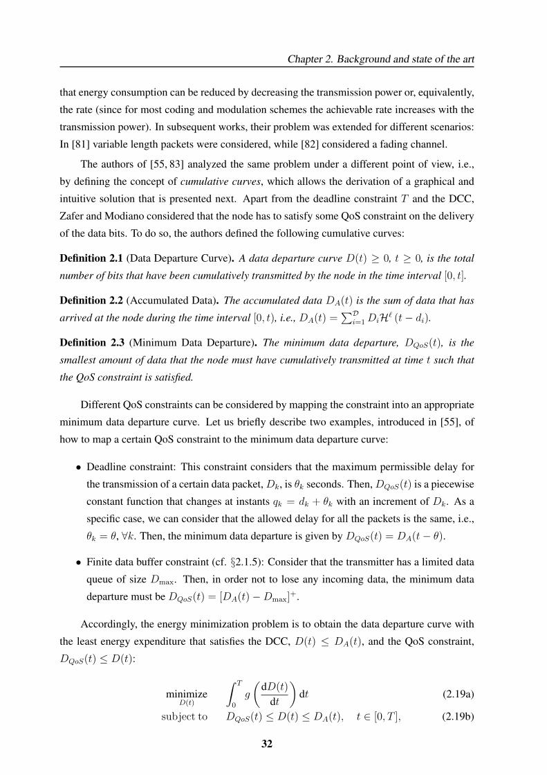
Chapter 2. Background and state of the art
that energy consumption can be reduced by decreasing the transmission power or, equivalently,
the rate (since for most coding and modulation schemes the achievable rate increases with the
transmission power). In subsequent works, their problem was extended for different scenarios:
In [81] variable length packets were considered, while [82] considered a fading channel.
The authors of [55, 83] analyzed the same problem under a different point of view, i.e.,
by defining the concept of cumulative curves, which allows the derivation of a graphical and
intuitive solution that is presented next. Apart from the deadline constraint T and the DCC,
Zafer and Modiano considered that the node has to satisfy some QoS constraint on the delivery
of the data bits. To do so, the authors defined the following cumulative curves:
Definition 2.1 (Data Departure Curve). A data departure curve D(t) ≥ 0, t ≥ 0, is the total
number of bits that have been cumulatively transmitted by the node in the time interval [0, t].
Definition 2.2 (Accumulated Data). The accumulated data DA(t) is the sum of data that has
arrived at the node during the time interval [0, t), i.e., DA(t) =∑D
i=1DiH` (t− di).
Definition 2.3 (Minimum Data Departure). The minimum data departure, DQoS(t), is the
smallest amount of data that the node must have cumulatively transmitted at time t such that
the QoS constraint is satisfied.
Different QoS constraints can be considered by mapping the constraint into an appropriate
minimum data departure curve. Let us briefly describe two examples, introduced in [55], of
how to map a certain QoS constraint to the minimum data departure curve:
• Deadline constraint: This constraint considers that the maximum permissible delay for
the transmission of a certain data packet, Dk, is θk seconds. Then, DQoS(t) is a piecewise
constant function that changes at instants qk = dk + θk with an increment of Dk. As a
specific case, we can consider that the allowed delay for all the packets is the same, i.e.,
θk = θ, ∀k. Then, the minimum data departure is given by DQoS(t) = DA(t− θ).
• Finite data buffer constraint (cf. §2.1.5): Consider that the transmitter has a limited data
queue of size Dmax. Then, in order not to lose any incoming data, the minimum data
departure must be DQoS(t) = [DA(t)−Dmax]+.
Accordingly, the energy minimization problem is to obtain the data departure curve with
the least energy expenditure that satisfies the DCC, D(t) ≤ DA(t), and the QoS constraint,
DQoS(t) ≤ D(t):
minimizeD(t)
∫ T
0
g
(dD(t)
dt
)dt (2.19a)
subject to DQoS(t) ≤ D(t) ≤ DA(t), t ∈ [0, T ], (2.19b)
32
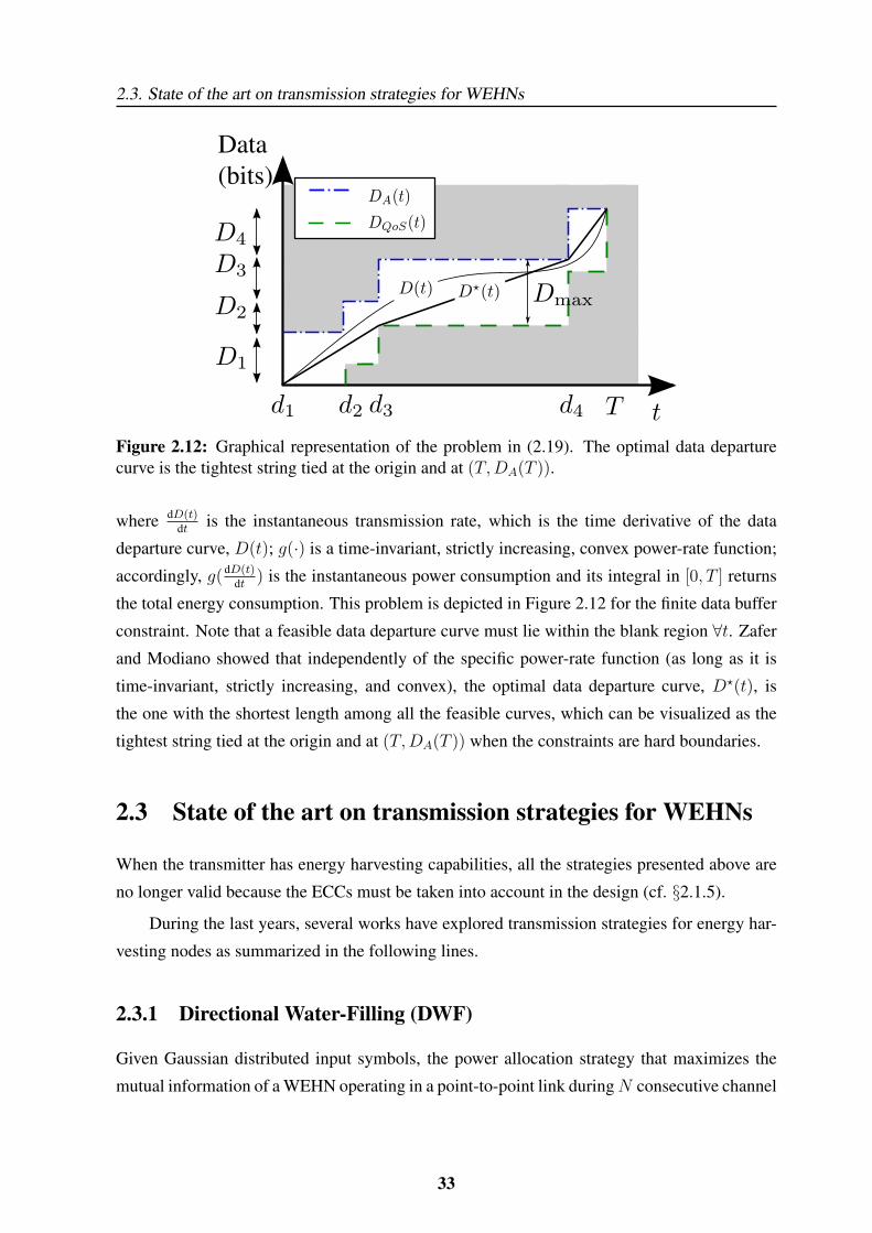
2.3. State of the art on transmission strategies for WEHNs
Figure 2.12: Graphical representation of the problem in (2.19). The optimal data departurecurve is the tightest string tied at the origin and at (T,DA(T )).
where dD(t)dt is the instantaneous transmission rate, which is the time derivative of the data
departure curve, D(t); g(·) is a time-invariant, strictly increasing, convex power-rate function;
accordingly, g(dD(t)dt ) is the instantaneous power consumption and its integral in [0, T ] returns
the total energy consumption. This problem is depicted in Figure 2.12 for the finite data buffer
constraint. Note that a feasible data departure curve must lie within the blank region ∀t. Zafer
and Modiano showed that independently of the specific power-rate function (as long as it is
time-invariant, strictly increasing, and convex), the optimal data departure curve, D?(t), is
the one with the shortest length among all the feasible curves, which can be visualized as the
tightest string tied at the origin and at (T,DA(T )) when the constraints are hard boundaries.
2.3 State of the art on transmission strategies for WEHNs
When the transmitter has energy harvesting capabilities, all the strategies presented above are
no longer valid because the ECCs must be taken into account in the design (cf. §2.1.5).
During the last years, several works have explored transmission strategies for energy har-
vesting nodes as summarized in the following lines.
2.3.1 Directional Water-Filling (DWF)
Given Gaussian distributed input symbols, the power allocation strategy that maximizes the
mutual information of a WEHN operating in a point-to-point link duringN consecutive channel
33
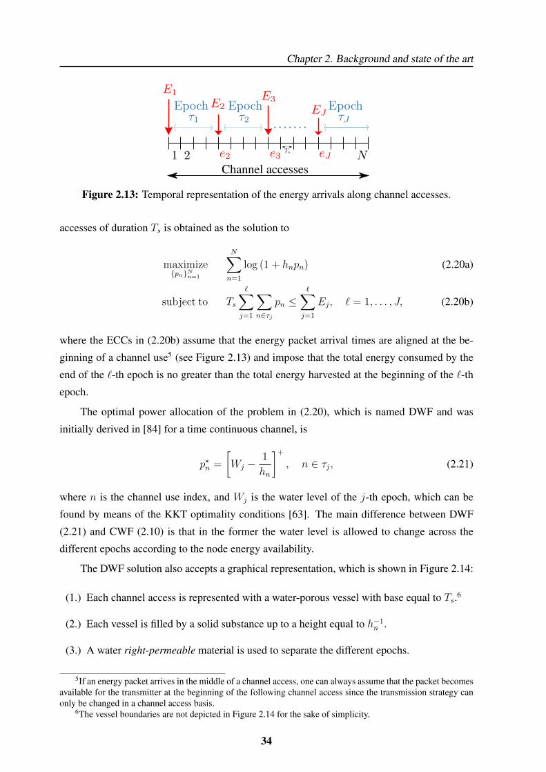
Chapter 2. Background and state of the art
Figure 2.13: Temporal representation of the energy arrivals along channel accesses.
accesses of duration Ts is obtained as the solution to
maximize{pn}Nn=1
N∑n=1
log (1 + hnpn) (2.20a)
subject to Ts∑j=1
∑n∈τj
pn ≤∑j=1
Ej, ` = 1, . . . , J, (2.20b)
where the ECCs in (2.20b) assume that the energy packet arrival times are aligned at the be-
ginning of a channel use5 (see Figure 2.13) and impose that the total energy consumed by the
end of the `-th epoch is no greater than the total energy harvested at the beginning of the `-th
epoch.
The optimal power allocation of the problem in (2.20), which is named DWF and was
initially derived in [84] for a time continuous channel, is
p?n =
[Wj −
1
hn
]+
, n ∈ τj, (2.21)
where n is the channel use index, and Wj is the water level of the j-th epoch, which can be
found by means of the KKT optimality conditions [63]. The main difference between DWF
(2.21) and CWF (2.10) is that in the former the water level is allowed to change across the
different epochs according to the node energy availability.
The DWF solution also accepts a graphical representation, which is shown in Figure 2.14:
(1.) Each channel access is represented with a water-porous vessel with base equal to Ts.6
(2.) Each vessel is filled by a solid substance up to a height equal to h−1n .
(3.) A water right-permeable material is used to separate the different epochs.
5If an energy packet arrives in the middle of a channel access, one can always assume that the packet becomesavailable for the transmitter at the beginning of the following channel access since the transmission strategy canonly be changed in a channel access basis.
6The vessel boundaries are not depicted in Figure 2.14 for the sake of simplicity.
34
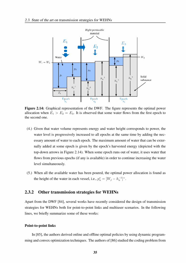
2.3. State of the art on transmission strategies for WEHNs
Figure 2.14: Graphical representation of the DWF. The figure represents the optimal powerallocation when E1 > E2 = E3. It is observed that some water flows from the first epoch tothe second one.
(4.) Given that water volume represents energy and water height corresponds to power, the
water level is progressively increased to all epochs at the same time by adding the nec-
essary amount of water to each epoch. The maximum amount of water that can be exter-
nally added at some epoch is given by the epoch’s harvested energy (depicted with the
top-down arrows in Figure 2.14). When some epoch runs out of water, it uses water that
flows from previous epochs (if any is available) in order to continue increasing the water
level simultaneously.
(5.) When all the available water has been poured, the optimal power allocation is found as
the height of the water in each vessel, i.e., p?n = [Wj − h−1n ]+.
2.3.2 Other transmission strategies for WEHNs
Apart from the DWF [84], several works have recently considered the design of transmission
strategies for WEHNs both for point-to-point links and multiuser scenarios. In the following
lines, we briefly summarize some of these works:
Point-to-point links
In [85], the authors derived online and offline optimal policies by using dynamic program-
ming and convex optimization techniques. The authors of [86] studied the coding problem from
35
Chapter 2. Background and state of the art
an information theoretic perspective. The transmission policy that maximizes the throughput
in a finite horizon for a finite battery capacity was derived in [87] assuming an infinite backlog
of data at the transmitter. In [88], different resource allocation strategies were evaluated and
compared by using real energy traces, which were collected in [35]. A learning theoretic ap-
proach was taken in [89], where data and energy arrivals were modeled as finite-state Markov
processes. Markov models were used in [90] to model the battery state of the node. Finally, the
stability and delay of the data queue were considered in [91] to derive the optimal transmission
policies.
The concept of cumulative curves, cf. §2.2.2, has been broadly used to derive optimal
transmission strategies for WEHNs. In this context, the authors of [92] considered dynamic
data packet arrivals and found the transmission strategy that minimizes the delivery time of all
data packets under the assumption of having infinite battery capacity. In [87], a node with finite
battery capacity was studied; however, it was considered that all the data packets are available
from the beginning of the transmission.
The works mentioned above consider that the transmission radiated power is the only en-
ergy sink of the node. In opposition, the works in [49, 93] derived optimal power allocation
strategies by using the power consumption model C1 in (2.5) for a time-static and fading con-
tinuous channel, respectively.
Multiuser communication systems
Several works have explored multiuser scenarios:
• Broadcast channel: The minimization of the transmission completion time for a WEHN
operating in a broadcast link was considered in [94–97]. References [94] and [95] as-
sumed infinite battery capacity, whereas, the authors of [96,97] found the rate scheduling
policy of the finite battery capacity case.
• Multiple access channel: The capacity region of a Gaussian multiple access channel
was considered in [98]. Under an offline approach, [99] proposed the power allocation
strategy that minimizes the transmission completion time. The stability of the packet
queues was studied in [100]. The authors of [101] proposed an online algorithm to max-
imize the long-term average channel throughput. Low-complexity scheduling policies to
maximize the sum throughput were derived in [102] without the knowledge of the power
harvesting profile.
• Relay and multi-hop channels: Two-hop communications were considered in [103–
109]. The optimal offline transmission scheme was proposed in [103] for the full-duplex
36
2.3. State of the art on transmission strategies for WEHNs
tow-hop relay channel. The optimal offline energy management policies for the source
and the relay that maximize the end-to-end throughput were studied in [104] by allowing
energy cooperation between the source and the relay. The authors of [109] proposed the
power allocation strategy that maximizes the system throughput over a finite number of
transmission time slots under conventional decode-and-forward relay (the relay retrans-
mits the signal in the consecutive time slots) and under the buffer-aided link adaptive
relaying (where the relay can retransmit the signal in any of the consecutive time slots).
The relay channel (with direct link between transmitter and destination) was studied
in [110–112].
• Cooperative transmissions: The authors of [45, 113] considered multiple energy har-
vesting sensors that transmit a shared common message to a distant base station and
studied the power allocation strategy in the different nodes that maximizes the total data
throughput.
• Interference channel: The power allocation that maximizes the sum throughput with
a given deadline for the two-user Gaussian interference channel with energy harvesting
transmitters was investigated in [114]. The two-user Gaussian interference channel was
studied in [115] by considering the cost of having the transmitter “on”, i.e., by using the
power consumption model C1 in (2.5).
In the following chapter, we have generalized the concept of cumulative curves introduced
by Zafer and Modiano in [83] to deal with energy harvesting at the transmitter, which has
allowed us to derive the scheduling strategy that minimizes the transmission completion time
while satisfying DCCs, ECCs, finite battery capacity constraint, and QoS constraints.
37

Chapter 3Transmission completion time minimization
for a WEHN
3.1 Introduction
This chapter considers a WEHN that acquires some data measurements over time, e.g., a sensor
that eventually or periodically senses a given process like temperature, humidity, etc. Each
measurement is digitalized in a sequence of bits that conform a data packet, which is stored in
the data buffer until it is transmitted. In practice, the data and energy buffers can only store
a finite amount of data and energy, respectively. In this context, this chapter investigates the
transmission strategy that minimizes the transmission completion time of a finite amount of
incoming data packets (the time by which all the data packets are transmitted), which arrive
dynamically over time as generally occurs in wireless sensor nodes.
As it is presented throughout this chapter, the transmission completion time minimization
problem for WEHNs is closely related to the energy minimization problem for non-harvesting
nodes. In particular, the concept of cumulative curves, which has been presented in §2.2.2, is a
useful tool to derive optimal transmission strategies for WEHNs.
As it has been presented in the previous chapter, given that energy harvesters are used to
power the transmitter(s), the minimization of the transmission completion time was consid-
ered in [84, 87, 92] for a point-to-point link and in [94, 96, 99] for multiuser scenarios, as it is
explained in more detail in the following lines.
The authors of [92] considered dynamic data packet arrivals and found the transmission
strategy that minimizes the transmission completion time by assuming an infinite battery ca-
pacity.
The optimal transmission policy for a finite battery capacity node was derived in [87] for
39
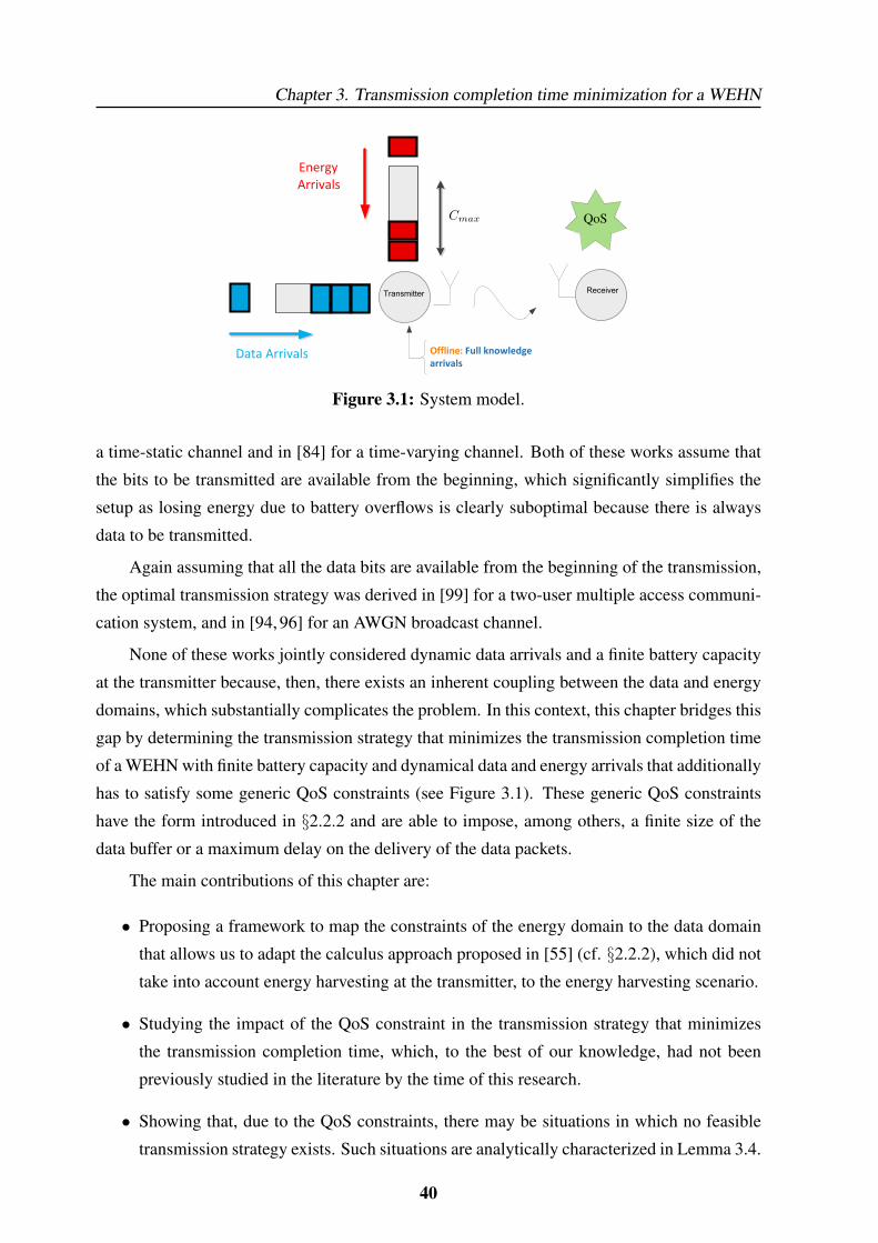
Chapter 3. Transmission completion time minimization for a WEHN
Energy
Arrivals
Data Arrivals
max
Offline: Full knowledge
arrivals
TransmitterReceiver
Figure 3.1: System model.
a time-static channel and in [84] for a time-varying channel. Both of these works assume that
the bits to be transmitted are available from the beginning, which significantly simplifies the
setup as losing energy due to battery overflows is clearly suboptimal because there is always
data to be transmitted.
Again assuming that all the data bits are available from the beginning of the transmission,
the optimal transmission strategy was derived in [99] for a two-user multiple access communi-
cation system, and in [94, 96] for an AWGN broadcast channel.
None of these works jointly considered dynamic data arrivals and a finite battery capacity
at the transmitter because, then, there exists an inherent coupling between the data and energy
domains, which substantially complicates the problem. In this context, this chapter bridges this
gap by determining the transmission strategy that minimizes the transmission completion time
of a WEHN with finite battery capacity and dynamical data and energy arrivals that additionally
has to satisfy some generic QoS constraints (see Figure 3.1). These generic QoS constraints
have the form introduced in §2.2.2 and are able to impose, among others, a finite size of the
data buffer or a maximum delay on the delivery of the data packets.
The main contributions of this chapter are:
• Proposing a framework to map the constraints of the energy domain to the data domain
that allows us to adapt the calculus approach proposed in [55] (cf. §2.2.2), which did not
take into account energy harvesting at the transmitter, to the energy harvesting scenario.
• Studying the impact of the QoS constraint in the transmission strategy that minimizes
the transmission completion time, which, to the best of our knowledge, had not been
previously studied in the literature by the time of this research.
• Showing that, due to the QoS constraints, there may be situations in which no feasible
transmission strategy exists. Such situations are analytically characterized in Lemma 3.4.
40
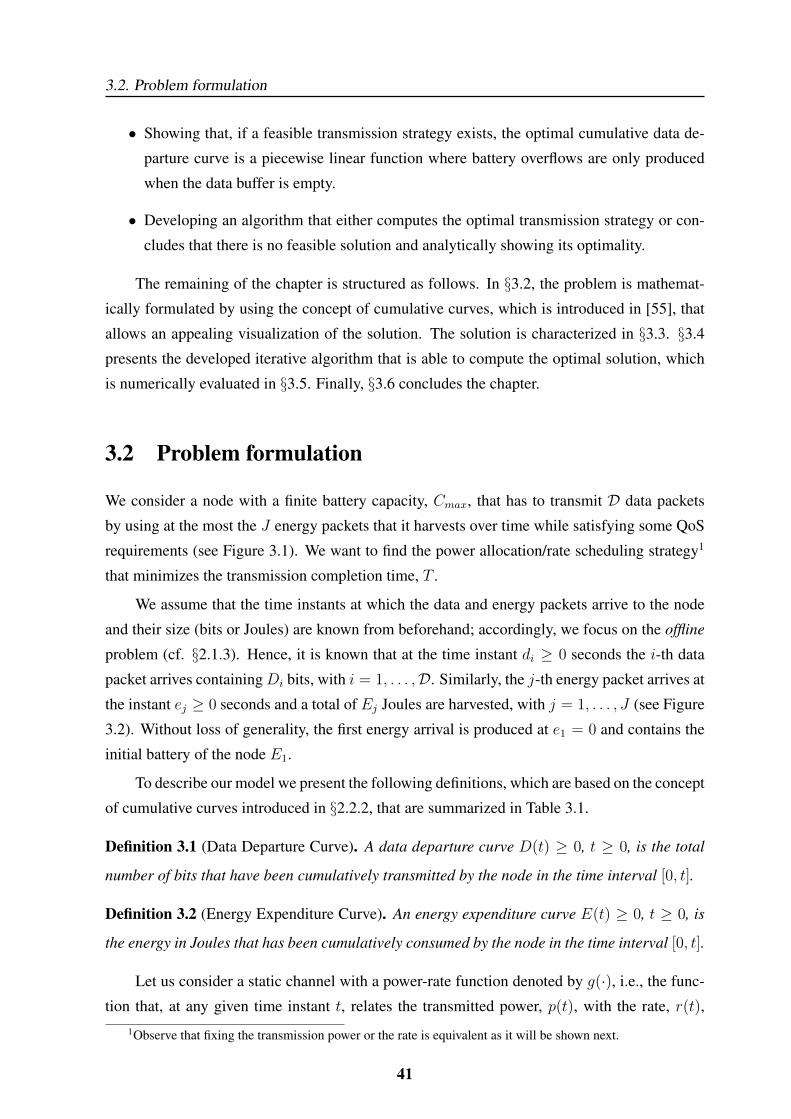
3.2. Problem formulation
• Showing that, if a feasible transmission strategy exists, the optimal cumulative data de-
parture curve is a piecewise linear function where battery overflows are only produced
when the data buffer is empty.
• Developing an algorithm that either computes the optimal transmission strategy or con-
cludes that there is no feasible solution and analytically showing its optimality.
The remaining of the chapter is structured as follows. In §3.2, the problem is mathemat-
ically formulated by using the concept of cumulative curves, which is introduced in [55], that
allows an appealing visualization of the solution. The solution is characterized in §3.3. §3.4
presents the developed iterative algorithm that is able to compute the optimal solution, which
is numerically evaluated in §3.5. Finally, §3.6 concludes the chapter.
3.2 Problem formulation
We consider a node with a finite battery capacity, Cmax, that has to transmit D data packets
by using at the most the J energy packets that it harvests over time while satisfying some QoS
requirements (see Figure 3.1). We want to find the power allocation/rate scheduling strategy1
that minimizes the transmission completion time, T .
We assume that the time instants at which the data and energy packets arrive to the node
and their size (bits or Joules) are known from beforehand; accordingly, we focus on the offline
problem (cf. §2.1.3). Hence, it is known that at the time instant di ≥ 0 seconds the i-th data
packet arrives containingDi bits, with i = 1, . . . ,D. Similarly, the j-th energy packet arrives at
the instant ej ≥ 0 seconds and a total of Ej Joules are harvested, with j = 1, . . . , J (see Figure
3.2). Without loss of generality, the first energy arrival is produced at e1 = 0 and contains the
initial battery of the node E1.
To describe our model we present the following definitions, which are based on the concept
of cumulative curves introduced in §2.2.2, that are summarized in Table 3.1.
Definition 3.1 (Data Departure Curve). A data departure curve D(t) ≥ 0, t ≥ 0, is the total
number of bits that have been cumulatively transmitted by the node in the time interval [0, t].
Definition 3.2 (Energy Expenditure Curve). An energy expenditure curve E(t) ≥ 0, t ≥ 0, is
the energy in Joules that has been cumulatively consumed by the node in the time interval [0, t].
Let us consider a static channel with a power-rate function denoted by g(·), i.e., the func-
tion that, at any given time instant t, relates the transmitted power, p(t), with the rate, r(t),1Observe that fixing the transmission power or the rate is equivalent as it will be shown next.
41
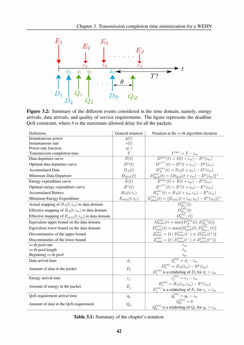
Chapter 3. Transmission completion time minimization for a WEHN
Figure 3.2: Summary of the different events considered in the time domain, namely, energyarrivals, data arrivals, and quality of service requirements. The figure represents the deadlineQoS constraint, where θ is the maximum allowed delay for all the packets.
Definition General notation Notation at the m-th algorithm iterationInstantaneous power p(t)Instantaneous rate r(t)Power-rate function g(·)Transmission completion time T T (m) = T − imData departure curve D(t) D(m)(t) = D(t+ im)−D?(im)
Optimal data departure curve D?(t) D?(m)
(t) = D?(t+ im)−D?(im)
Accumulated Data DA(t) D(m)A (t) = DA(t+ im)−D?(im)
Minimum Data Departure DQoS(t) D(m)QoS(t) = {DQoS(t+ im)−D?(im)}+
Energy expenditure curve E(t) E(m)(t) = E(t+ im)− E?(im)
Optimal energy expenditure curve E?(t) E?(m)
(t) = E?(t+ im)− E?(im)
Accumulated Battery BA(t; tx) B(m)A (t) = BA(t+ im; im)− E?(im)
Minimum Energy Expenditure Emin(t; tx) E(m)min(t) = {Emin(t+ im; im)− E?(im)}+
Actual mapping of BA(t; im) to data domain D(m)BA
(t)
Effective mapping of BA(t; im) to data domain D(m)BA
(t)
Effective mapping of Emin(t; im) to data domain D(m)Emin
(t)
Equivalent upper bound on the data domain D(m)max(t) = min{D(m)
A (t), D(m)BA
(t)}Equivalent lower bound on the data domain D
(m)min(t) = max{D(m)
QoS(t), D(m)Emin
(t)}Discontinuities of the upper bound Z(m)
max = {t |D(m)max(t−) 6= D
(m)max(t+)}
Discontinuities of the lower bound Z(m)min = {t |D(m)
min(t−) 6= D(m)min(t+)}
m-th pool rate rmm-th pool length `mBeginning m-th pool im
Data arrival time di d(m)i = di − im
Amount of data in the packet DiD
(m)0 = DA(im)−D?(im)
D(m)i is a relabeling of Di for di > im
Energy arrival time ej e(m)j = ej − im
Amount of energy in the packet EjE
(m)1 = BA(im; im)− E?(im)
E(m)j is a relabeling of Ej for ej > im
QoS requirement arrival time qk q(m)k = qk − im
Amount of data in the QoS requirement QkQ
(m)0 = 0
Q(m)k is a relabeling of Qk for qk > im
Table 3.1: Summary of the chapter’s notation.
42
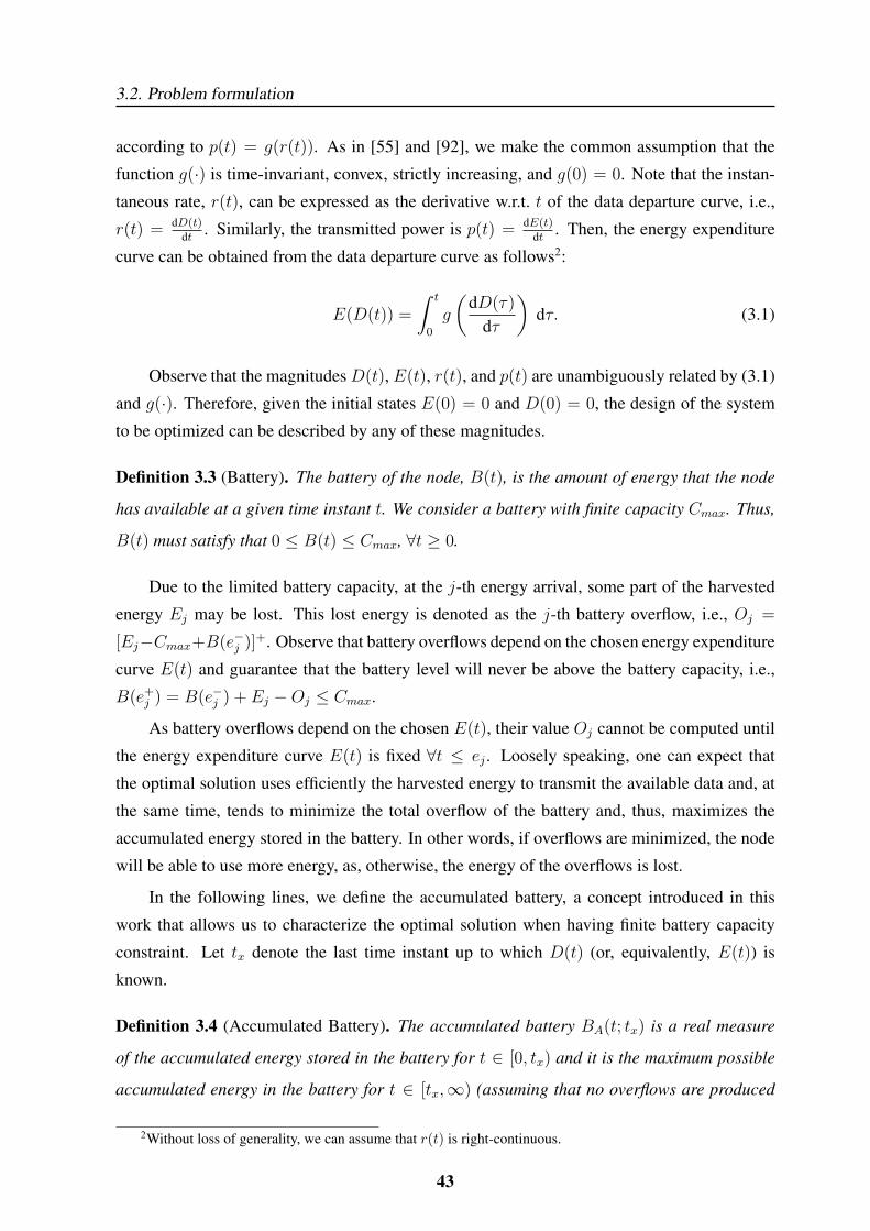
3.2. Problem formulation
according to p(t) = g(r(t)). As in [55] and [92], we make the common assumption that the
function g(·) is time-invariant, convex, strictly increasing, and g(0) = 0. Note that the instan-
taneous rate, r(t), can be expressed as the derivative w.r.t. t of the data departure curve, i.e.,
r(t) = dD(t)dt . Similarly, the transmitted power is p(t) = dE(t)
dt . Then, the energy expenditure
curve can be obtained from the data departure curve as follows2:
E(D(t)) =
∫ t
0
g
(dD(τ)
dτ
)dτ. (3.1)
Observe that the magnitudesD(t), E(t), r(t), and p(t) are unambiguously related by (3.1)
and g(·). Therefore, given the initial states E(0) = 0 and D(0) = 0, the design of the system
to be optimized can be described by any of these magnitudes.
Definition 3.3 (Battery). The battery of the node, B(t), is the amount of energy that the node
has available at a given time instant t. We consider a battery with finite capacity Cmax. Thus,
B(t) must satisfy that 0 ≤ B(t) ≤ Cmax, ∀t ≥ 0.
Due to the limited battery capacity, at the j-th energy arrival, some part of the harvested
energy Ej may be lost. This lost energy is denoted as the j-th battery overflow, i.e., Oj =
[Ej−Cmax+B(e−j )]+. Observe that battery overflows depend on the chosen energy expenditure
curve E(t) and guarantee that the battery level will never be above the battery capacity, i.e.,
B(e+j ) = B(e−j ) + Ej −Oj ≤ Cmax.
As battery overflows depend on the chosen E(t), their value Oj cannot be computed until
the energy expenditure curve E(t) is fixed ∀t ≤ ej . Loosely speaking, one can expect that
the optimal solution uses efficiently the harvested energy to transmit the available data and, at
the same time, tends to minimize the total overflow of the battery and, thus, maximizes the
accumulated energy stored in the battery. In other words, if overflows are minimized, the node
will be able to use more energy, as, otherwise, the energy of the overflows is lost.
In the following lines, we define the accumulated battery, a concept introduced in this
work that allows us to characterize the optimal solution when having finite battery capacity
constraint. Let tx denote the last time instant up to which D(t) (or, equivalently, E(t)) is
known.
Definition 3.4 (Accumulated Battery). The accumulated battery BA(t; tx) is a real measure
of the accumulated energy stored in the battery for t ∈ [0, tx) and it is the maximum possible
accumulated energy in the battery for t ∈ [tx,∞) (assuming that no overflows are produced
2Without loss of generality, we can assume that r(t) is right-continuous.
43
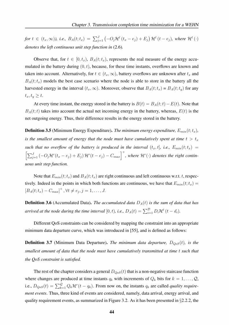
Chapter 3. Transmission completion time minimization for a WEHN
for t ∈ (tx,∞)), i.e., BA(t; tx) =∑J
j=1
(−OjH` (tx − ej) + Ej
)H` (t− ej), where H` (·)
denotes the left continuous unit step function in (2.6).
Observe that, for t ∈ [0, tx), BA(t; tx), represents the real measure of the energy accu-
mulated in the battery during (0, t), because, for these time instants, overflows are known and
taken into account. Alternatively, for t ∈ (tx,∞), battery overflows are unknown after tx and
BA(t; tx) models the best case scenario where the node is able to store in the battery all the
harvested energy in the interval (tx,∞). Moreover, observe that BA(t; tx) = BA(t; ty) for any
tx, ty ≥ t.
At every time instant, the energy stored in the battery is B(t) = BA(t; t)−E(t). Note that
BA(t; t) takes into account the actual net incoming energy in the battery, whereas, E(t) is the
net outgoing energy. Thus, their difference results in the energy stored in the battery.
Definition 3.5 (Minimum Energy Expenditure). The minimum energy expenditure, Emin(t; tx),
is the smallest amount of energy that the node must have cumulatively spent at time t > tx
such that no overflow of the battery is produced in the interval (tx, t], i.e., Emin(t; tx) =[∑Jj=1 (−OjHr(tx − ej) + Ej)Hr(t− ej)− Cmax
]+
, where Hr(·) denotes the right contin-
uous unit step function.
Note thatEmin(t; tx) andBA(t; tx) are right continuous and left continuous w.r.t. t, respec-
tively. Indeed in the points in which both functions are continuous, we have that Emin(t; tx) =
[BA(t; tx)− Cmax]+ ,∀t 6= ej, j = 1, . . . , J.
Definition 3.6 (Accumulated Data). The accumulated data DA(t) is the sum of data that has
arrived at the node during the time interval [0, t), i.e., DA(t) =∑D
i=1 DiH` (t− di).
Different QoS constraints can be considered by mapping the constraint into an appropriate
minimum data departure curve, which was introduced in [55], and is defined as follows:
Definition 3.7 (Minimum Data Departure). The minimum data departure, DQoS(t), is the
smallest amount of data that the node must have cumulatively transmitted at time t such that
the QoS constraint is satisfied.
The rest of the chapter considers a generalDQoS(t) that is a non-negative staircase function
where changes are produced at time instants qk with increments of Qk bits for k = 1, . . . ,Q,
i.e., DQoS(t) =∑Q
k=1QkHr(t − qk). From now on, the instants qk are called quality require-
ment events. Thus, three kind of events are considered, namely, data arrival, energy arrival, and
quality requirement events, as summarized in Figure 3.2. As it has been presented in §2.2.2, the
44
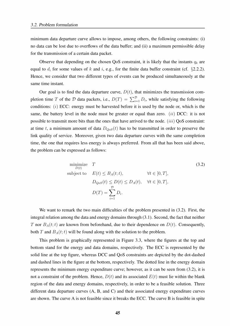
3.2. Problem formulation
minimum data departure curve allows to impose, among others, the following constraints: (i)
no data can be lost due to overflows of the data buffer; and (ii) a maximum permissible delay
for the transmission of a certain data packet.
Observe that depending on the chosen QoS constraint, it is likely that the instants qk are
equal to di for some values of k and i, e.g., for the finite data buffer constraint (cf. §2.2.2).
Hence, we consider that two different types of events can be produced simultaneously at the
same time instant.
Our goal is to find the data departure curve, D(t), that minimizes the transmission com-
pletion time T of the D data packets, i.e., D(T ) =∑D
i=1Di, while satisfying the following
conditions: (i) ECC: energy must be harvested before it is used by the node or, which is the
same, the battery level in the node must be greater or equal than zero. (ii) DCC: it is not
possible to transmit more bits than the ones that have arrived to the node. (iii) QoS constraint:
at time t, a minimum amount of data DQoS(t) has to be transmitted in order to preserve the
link quality of service. Moreover, given two data departure curves with the same completion
time, the one that requires less energy is always preferred. From all that has been said above,
the problem can be expressed as follows:
minimizeD(t)
T (3.2)
subject to E(t) ≤ BA(t; t), ∀t ∈ [0, T ],
DQoS(t) ≤ D(t) ≤ DA(t), ∀t ∈ [0, T ],
D(T ) =D∑i=1
Di.
We want to remark the two main difficulties of the problem presented in (3.2). First, the
integral relation among the data and energy domains through (3.1). Second, the fact that neither
T nor BA(t; t) are known from beforehand, due to their dependence on D(t). Consequently,
both T and BA(t; t) will be found along with the solution to the problem.
This problem is graphically represented in Figure 3.3, where the figures at the top and
bottom stand for the energy and data domains, respectively. The ECC is represented by the
solid line at the top figure, whereas DCC and QoS constraints are depicted by the dot-dashed
and dashed lines in the figure at the bottom, respectively. The dotted line in the energy domain
represents the minimum energy expenditure curve; however, as it can be seen from (3.2), it is
not a constraint of the problem. Hence, D(t) and its associated E(t) must lie within the blank
region of the data and energy domains, respectively, in order to be a feasible solution. Three
different data departure curves (A, B, and C) and their associated energy expenditure curves
are shown. The curve A is not feasible since it breaks the ECC. The curve B is feasible in spite
45
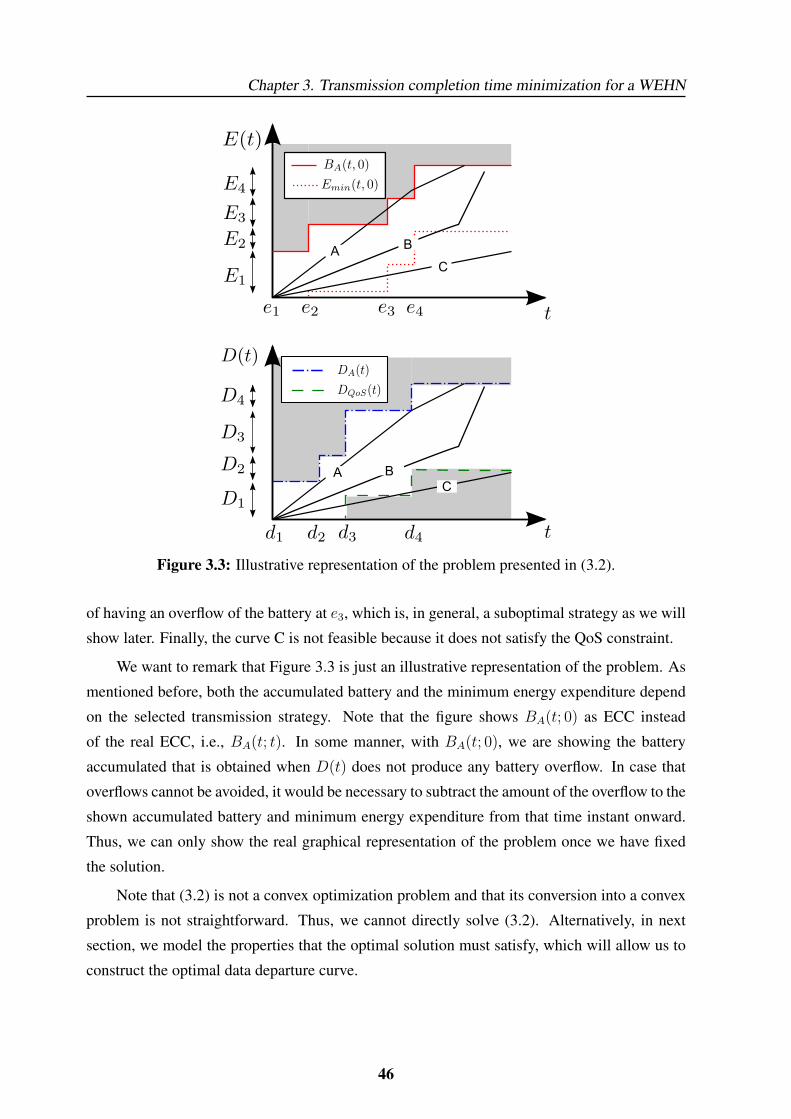
Chapter 3. Transmission completion time minimization for a WEHN
AB
A B
C
C
Figure 3.3: Illustrative representation of the problem presented in (3.2).
of having an overflow of the battery at e3, which is, in general, a suboptimal strategy as we will
show later. Finally, the curve C is not feasible because it does not satisfy the QoS constraint.
We want to remark that Figure 3.3 is just an illustrative representation of the problem. As
mentioned before, both the accumulated battery and the minimum energy expenditure depend
on the selected transmission strategy. Note that the figure shows BA(t; 0) as ECC instead
of the real ECC, i.e., BA(t; t). In some manner, with BA(t; 0), we are showing the battery
accumulated that is obtained when D(t) does not produce any battery overflow. In case that
overflows cannot be avoided, it would be necessary to subtract the amount of the overflow to the
shown accumulated battery and minimum energy expenditure from that time instant onward.
Thus, we can only show the real graphical representation of the problem once we have fixed
the solution.
Note that (3.2) is not a convex optimization problem and that its conversion into a convex
problem is not straightforward. Thus, we cannot directly solve (3.2). Alternatively, in next
section, we model the properties that the optimal solution must satisfy, which will allow us to
construct the optimal data departure curve.
46
3.3. Properties of the optimal solution
3.3 Properties of the optimal solution
As pointed out previously, in this section we will characterize the optimal data departure curve,
D?(t), and its associated energy expenditure curve, E?(t), for the problem (3.2):
Problem 3.1 (Transmission Without Events). Consider that the optimal departure curve is
known up to t1 and that we want to characterize its optimal behaviour in the time interval
(t1, t2) where there are no changes in DA(t), BA(t; t1), and DQoS(t). We also consider that
the data departure curve at the boundary of the intervals is D(t1) and D(t2), respectively, and
that these two points satisfy the data, energy, and QoS constraints.
Lemma 3.1. In Problem 3.1, D?(t) is a straight line where the slope, or, equivalently, the
transmission rate, is constant and equal to r(t) = D(t2)−D(t1)t2−t1 , ∀t ∈ (t1, t2).
Proof: The proof follows from the integral version of Jensen’s inequality in a similar
way to the BT-problem in [55].
Corollary 3.1. Lemma 3.1 implies that D?(t) is a piecewise linear function such that its slope,
which is equivalent to the transmission rate, can only change either at ej , di or qk.
From the previous lemma and corollary, it follows that constant rate transmission saves en-
ergy due to the convexity of the power-rate function g(·). However, constant rate transmission
is not optimal when a battery overflow is produced because the energy saved due to constant
rate transmission is lower than the energy lost in the overflow. Consequently, the optimal solu-
tion increases the rate before the overflow until either there is no overflow or the data buffer is
empty, as shown in the following lemma and its subsequent proof:
Lemma 3.2. Under the optimal policy, battery overflows may only be produced when there is
no data to be transmitted.
Proof: See appendix 3.A.1.
The following lemma states that by the end of the transmission the battery must be empty,
otherwise, transmission could have been finished earlier by transmitting at a higher rate.
Lemma 3.3. The optimal solution must satisfy that, at the instant T at which all the data has
been transmitted, the energy expenditure is equal to the accumulated battery, i.e., E?(T ) =
BA(T ;T ).
47
Chapter 3. Transmission completion time minimization for a WEHN
Proof: The proof follows in a similar way to the proof of Lemma 5 in [87].
In the remainder of the chapter, the term pool denotes each of the time intervals of D?(t)
at which transmission is done at constant rate. We define M as the total number of pools of the
optimal solution, i.e., the number of linear pieces of D?(t). Note that M is unknown a priori.
Consequently, solving the problem in (3.2) is equivalent to determining the rate rm and length
`m of each pool, i.e., {rm, `m}Mm=1. To do so, we have developed an iterative algorithm that, at
the m-th iteration, determines the rate and duration of the m-th pool, i.e., {rm, `m}. We denote
im as the instant at which them-th pool begins, i.e., im =∑m−1
p=1 `p, where by definition i1 = 0.
The algorithm ends when all data has been efficiently transmitted. With this, M , T , BA(t;T ),
and D?(t) are found.
To simplify the complexity of our algorithm, at the beginning of the m-th iteration3, the
origin of coordinates is moved to the point (im, D?(im)). To be coherent with the vertical
and horizontal displacement of the origin of coordinates, the data and energy constraints in
(3.2) must be vertically rescaled by D?(im) and E?(im), respectively, and temporally dis-
placed by im. In the remainder of the chapter, a super-index (m) above a variable (B(m)A (t),
D(m)A (t), D(m)
QoS(t), and E(m)min(t)) denotes that it is the rescaled version at the m-th iteration4,
e.g., B(m)A (t) = BA(t+ im; im)− E?(im)5.
From the structure of the problem in (3.2), it is expected that it may not have a feasible
solution whenever the node has to fulfill very tight QoS requirements, while, at the same time,
it does not harvest enough energy to transmit all the required data. The following lemma is
checked at every iteration of our proposed algorithm to determine whether the problem in (3.2)
has a feasible solution or not.
Lemma 3.4. The problem (3.2) does not have a feasible solution whenever
D(m)QoS(q
(m)k ) > q
(m)k g−1
(B
(m)A (q
(m)k )/q
(m)k
), (3.3)
for some quality requirement event q(m)k ∈ (0, T (m))6.
Proof: Whenever we encounter that the problem does not have a feasible solution is
because, at some quality requirement event q(m)k , it is not possible to fulfill all the constraints.
Let D(t) be the data departure curve that transmits the maximum amount of data in the in-
terval [0, q(m)k ], i.e., D(t) = g−1
(B
(m)A (q
(m)k )/q
(m)k
)t. Note that this curve has constant rate,
3Note that D?(t) is known in [0, im].4The relations among the iteration specific and general versions of the variables are given in Table 3.1.5We have dropped the second argument in B(m)
A (t) and E(m)min(t) since within the m-th iteration, the second
argument, which denotes the last instant at which the solution is known, is always im.6Where X(m) = X − im is the rescaled version of some temporal variable X at the m-th iteration (see Table
3.1).
48
3.3. Properties of the optimal solution
empties the battery at q(m)k , and that the constrains are not necessarily satisfied. If, at some
q(m)k ∈ (0, T (m)), the QoS constraint requires more than g−1
(B
(m)A (q
(m)k )/q
(m)k
)q
(m)k bits to be
transmitted, then the problem does not have a feasible solution.
If there is no q(m)k ∈ (0, T (m)) that satisfies Lemma 3.4, then the problem still may have a
feasible solution and at least another pool, i.e., {rm, `m}, can be determined. In this context in
the next subsection, we model how the rate changes must be produced in order to be optimal.
3.3.1 Constraints mapping into the data domain for a given pool
Within an algorithm iteration, the ECC can be mapped to the data domain, hence, allowing us
to merge both constraints to the most restrictive constraint. Let us consider that the algorithm
is at the beginning of the m-th iteration, i.e., the optimal solution is known up to im, where the
rate rm and length `m of the m-th pool must be determined. Given that transmission must be
done at constant rate/power, the maximum amount of data that can be transmitted at a certain
time instant ty due to the ECC is g−1(py)ty, where py = B(m)A (ty)/ty.7 With this, at the instant
ty, the upper bound on the energy expenditure curve has been mapped to an upper bound on
the data departure curve, as shown in Figure 3.4 for the instants t1 and t2. By applying this
procedure at all time instants ty ∈ (0, T (m)), we can map the whole upper bound in the energy
domain to an upper bound in the data domain, which we denote by D(m)BA
(t) = g−1(B(m)A (t)/t)t
and call actual mapping. However, doing this computation for each time instant has a high
computational cost. In summary, if a data departure curve that transmits at constant rate, i.e.,
D(m)(t) = rmt, satisfies that D(m)(t) ≤ D(m)BA
(t),∀t, then it also satisfies the ECCs.
The cost associated with the computation of D(m)BA
(t) can be reduced by noting that it is
suboptimal that D(m)(t) reaches the actual mapping at any time instant t1 that is not an event,
i.e., t1 6= d(m)i , t1 6= e
(m)j , and t1 6= q
(m)k , ∀i, j, k. This is clearly seen in Figure 3.4. Observe
that if D(m)(t1) = D(m)BA
(t1), then the battery is empty at t1, i.e., E(m)(t1) = B(m)A (t1), which
follows from the definition of the actual mapping. Consequently, in order to satisfy the ECCs,
the rate at t+1 must be zero as no energy arrival is produced at t1. From Corollary 3.1, we know
that this rate change is suboptimal and, therefore, the data departure curve can only reach the
actual mapping in some event. Thus, to reduce the computational complexity of the actual
mapping, we can compute the value of the mapping only at the aforementioned events and
assign a constant value in the interval between events. In the rest of the chapter, we refer to this
mapping as effective mapping, i.e., D(m)BA
(t). Note that the effective mapping is an upper bound
of the actual mapping. However, we want to remark that by using the effective mapping, we are
7Note that for the constraints mapping it is not necessary that py satisfies the constraints. The constraintsfulfillment is enforced by the algorithm that computes the optimal solution, which is explained in Section 3.4.
49
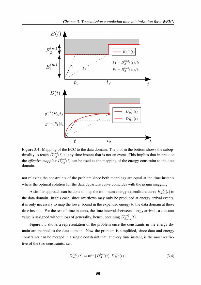
Chapter 3. Transmission completion time minimization for a WEHN
x
x
Figure 3.4: Mapping of the ECC to the data domain. The plot in the bottom shows the subop-timality to reach D(m)
BA(t) at any time instant that is not an event. This implies that in practice
the effective mapping D(m)BA
(t) can be used as the mapping of the energy constraint to the datadomain.
not relaxing the constraints of the problem since both mappings are equal at the time instants
where the optimal solution for the data departure curve coincides with the actual mapping.
A similar approach can be done to map the minimum energy expenditure curve E(m)min(t) to
the data domain. In this case, since overflows may only be produced at energy arrival events,
it is only necessary to map the lower bound in the expended energy to the data domain at these
time instants. For the rest of time instants, the time intervals between energy arrivals, a constant
value is assigned without loss of generality, hence, obtaining D(m)Emin
(t).
Figure 3.5 shows a representation of the problem once the constraints in the energy do-
main are mapped to the data domain. Now the problem is simplified, since data and energy
constraints can be merged in a single constraint that, at every time instant, is the most restric-
tive of the two constraints, i.e.,
D(m)max(t) = min{D(m)
A (t), D(m)BA
(t)}. (3.4)
50
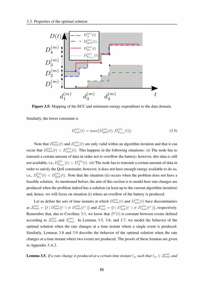
3.3. Properties of the optimal solution
x
x
x
x
x
x
Figure 3.5: Mapping of the ECC and minimum energy expenditure to the data domain.
Similarly, the lower constraint is
D(m)min(t) = max{D(m)
QoS(t), D(m)Emin
(t)}. (3.5)
Note that D(m)max(t) and D(m)
min(t) are only valid within an algorithm iteration and that it can
occur that D(m)max(t) < D
(m)min(t). This happens in the following situations: (i) The node has to
transmit a certain amount of data in order not to overflow the battery; however, this data is still
not available, i.e, D(m)Emin
(t) > D(m)A (t). (ii) The node has to transmit a certain amount of data in
order to satisfy the QoS constraint; however, it does not have enough energy available to do so,
i.e., D(m)BA
(t) < D(m)QoS(t). Note that the situation (ii) occurs when the problem does not have a
feasible solution. As mentioned before, the aim of this section is to model how rate changes are
produced when the problem indeed has a solution (at least up to the current algorithm iteration)
and, hence, we will focus on situation (i) where an overflow of the battery is produced.
Let us define the sets of time instants at which D(m)max(t) and D(m)
min(t) have discontinuities
as Z(m)max = {t |D(m)
max(t−) 6= D(m)max(t+)} and Z(m)
min = {t |D(m)min(t−) 6= D
(m)min(t+)}, respectively.
Remember that, due to Corollary 3.1, we know that D?(t) is constant between events defined
according to Z(m)max and Z(m)
min. In Lemmas 3.5, 3.6, and 3.7, we model the behavior of the
optimal solution when the rate changes at a time instant where a single event is produced.
Similarly, Lemmas 3.8 and 3.9 describe the behavior of the optimal solution when the rate
changes at a time instant where two events are produced. The proofs of these lemmas are given
in Appendix 3.A.2.
Lemma 3.5. If a rate change is produced at a certain time instant `m such that `m ∈ Z(m)max and
51
Chapter 3. Transmission completion time minimization for a WEHN
`m /∈ Z(m)min, then D?(m)
(`m) = D(m)max(`−m) and the rate increases, rm < rm+1.
Lemma 3.6. If a rate change is produced at the time instant `m such that `m /∈ Z(m)max, `m ∈
Z(m)min and D(m)
max(`m) ≥ D(m)min(`+
m), then D?(m)(`m) = D
(m)min(`+
m) and the rate decreases, rm >
rm+1.
Lemma 3.7. If a rate change is produced at a certain time instant `m such that `m /∈ Z(m)max,
`m ∈ Z(m)min and D(m)
max(`m) < D(m)min(`+
m), then an overflow of the battery is produced at `m,
D?(m)(`m) = D
(m)max(`m) and the rate is zero until the next data arrival event, rm+1 = 0.
Lemma 3.8. If a rate change is produced at a certain time instant `m such that `m ∈ Z(m)max,
`m ∈ Z(m)min, and D(m)
max(`−m) ≥ D(m)min(`+
m), then either D?(m)(`m) = D
(m)max(`−m) and the rate
increases, or D?(m)(`m) = D
(m)min(`+
m) and the rate decreases.
Lemma 3.9. If a rate change is produced at a certain time instant `m such that `m ∈ Z(m)max,
`m ∈ Z(m)min, and D(m)
max(`−m) < D(m)min(`+
m), then an overflow of the battery is produced at `m,
D?(m)(`m) = D
(m)max(`−m) and the rate can either increase or decrease.
By using these lemmas, we are able to construct an algorithm, which is presented in the
next section, that iteratively finds the optimal solution, or concludes that there is no feasible
solution.
3.4 Optimal data departure curve construction
In this section, we describe the developed algorithm that is able to either construct D?(t) or,
alternatively, conclude that the problem in (3.2) does not have a feasible solution. As stated in
Corollary 3.1, the optimal data departure curve is a piecewise linear function. As previously
explained, the developed algorithm follows an iterative process where, at them-th iteration, the
duration, `m, and rate, rm, of a pool are determined. We will focus on the explanation of the
m-th iteration since all the other iterations follow the same approach.
As shown in Figure 3.6, the algorithm is composed by three main blocks. The first block,
named checkSolution, determines the existence of solution in the current iteration by checking
the condition in Lemma 3.4. If the problem does not have a solution, the algorithm ends.
Otherwise, the algorithm proceeds to the subsequent blocks to determine the rate and length of
the pool.
The second block, named checkFinish, checks whether it is possible to transmit all the
remaining data by using all the available energy at constant rate. This block is necessary
52
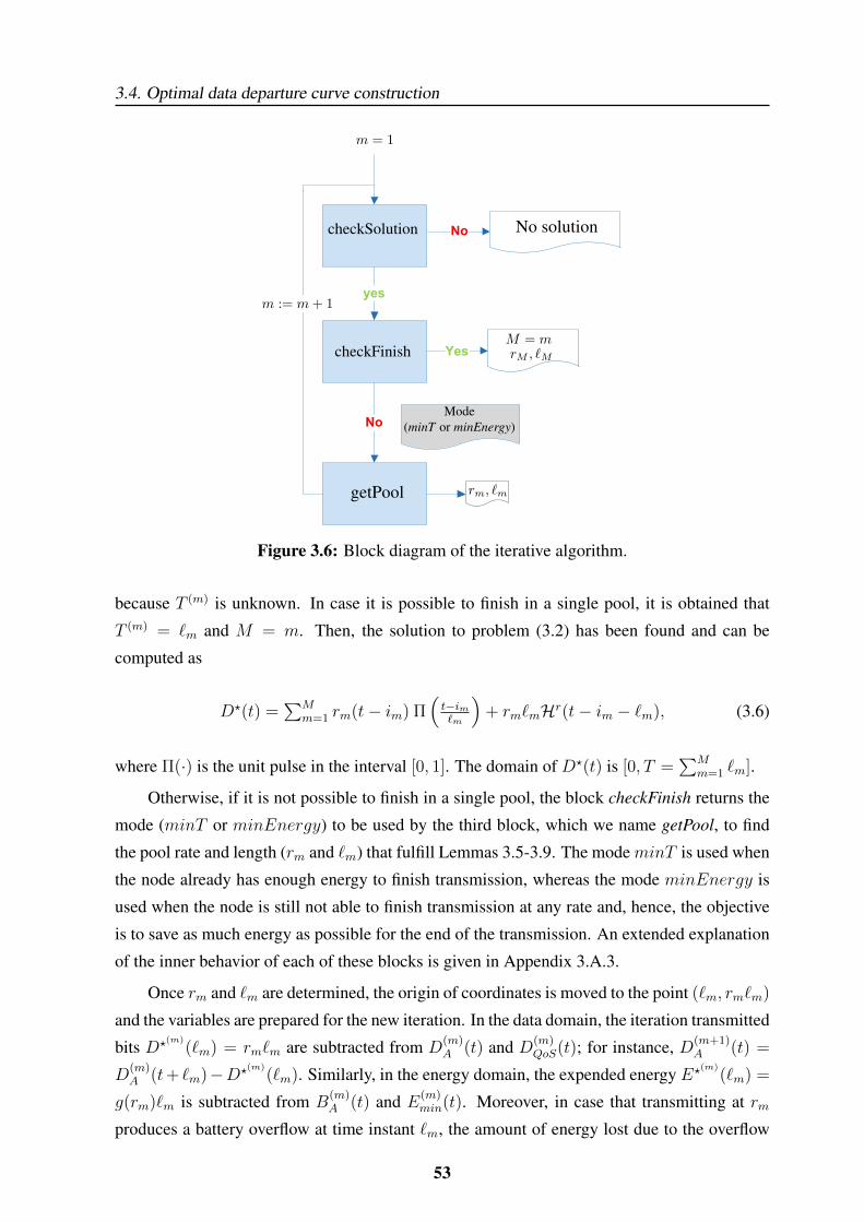
3.4. Optimal data departure curve construction
Yes
No
yes
No
Figure 3.6: Block diagram of the iterative algorithm.
because T (m) is unknown. In case it is possible to finish in a single pool, it is obtained that
T (m) = `m and M = m. Then, the solution to problem (3.2) has been found and can be
computed as
D?(t) =∑M
m=1 rm(t− im) Π(t−im`m
)+ rm`mHr(t− im − `m), (3.6)
where Π(·) is the unit pulse in the interval [0, 1]. The domain of D?(t) is [0, T =∑M
m=1 `m].
Otherwise, if it is not possible to finish in a single pool, the block checkFinish returns the
mode (minT or minEnergy) to be used by the third block, which we name getPool, to find
the pool rate and length (rm and `m) that fulfill Lemmas 3.5-3.9. The modeminT is used when
the node already has enough energy to finish transmission, whereas the mode minEnergy is
used when the node is still not able to finish transmission at any rate and, hence, the objective
is to save as much energy as possible for the end of the transmission. An extended explanation
of the inner behavior of each of these blocks is given in Appendix 3.A.3.
Once rm and `m are determined, the origin of coordinates is moved to the point (`m, rm`m)
and the variables are prepared for the new iteration. In the data domain, the iteration transmitted
bits D?(m)(`m) = rm`m are subtracted from D
(m)A (t) and D(m)
QoS(t); for instance, D(m+1)A (t) =
D(m)A (t+ `m)−D?(m)
(`m). Similarly, in the energy domain, the expended energy E?(m)(`m) =
g(rm)`m is subtracted from B(m)A (t) and E(m)
min(t). Moreover, in case that transmitting at rmproduces a battery overflow at time instant `m, the amount of energy lost due to the overflow
53
Chapter 3. Transmission completion time minimization for a WEHN
is also subtracted from these variables. Finally, the mapping to the data domain is recalculated
for the iteration m+ 1 and the whole procedure starts again to determine rm+1 and lm+1.
There are two possible reasons for which the algorithm ends: (i) At some iteration, Lemma
3.4 is satisfied and, hence, the problem does not have solution. (ii) All the data has been
transmitted and the optimal data departure curve has been obtained as given in (3.6).
The algorithm optimality is summarized in the following theorem and its subsequent
proof:
Theorem 3.1. The algorithm presented in this section constructs the optimal data departure
curve, D?(t), for the problem (3.2).
Proof: See appendix 3.A.3.4.
3.5 Results
To the best of our knowledge there is no other algorithm in the literature that considers alto-
gether the ECC, DCC, the QoS constraint and the finite battery capacity. Therefore, in order
to get some insights on the gain obtained with our proposed solution, we have developed a
suboptimal ad-hoc strategy, namely, the Empty Buffers Strategy (EBS), that tries to empty the
buffers as soon as possible, i.e., it looks for the time instant at which the next arrival (energy
or data) is produced and tries to transmit at a constant rate so that the corresponding buffer is
emptied by the time of the corresponding arrival.
The left y-axis of Figure 3.7 compares the normalized mean minimum T along a total of
1000 iterations, where at each iteration the data and energy arrivals are randomly generated
following a uniform distribution. The amount of energy in each of the packets is normalized
according to the total harvested energy which varies along the x-axis. The right y-axis shows
the percentage of iterations in which there exists a feasible solution to (3.2). As shown in
Figure 3.7, our proposed optimal algorithm substantially reduces the mean minimum T . If
feasible solutions exist, the optimal algorithm finds the one that minimizes T ; however, for
some arrival profiles, the EBS is not able to find any feasible solution in spite of its existence.
Note that the EBS performs worse than the optimal strategy because it changes the rate at
every packet arrival without checking whether constant power transmission is feasible between
two arrivals, which would consume less energy. As a result of this extra energy consumption,
the mean minimum T is higher and the probability of finding a feasible solution decreases.
54
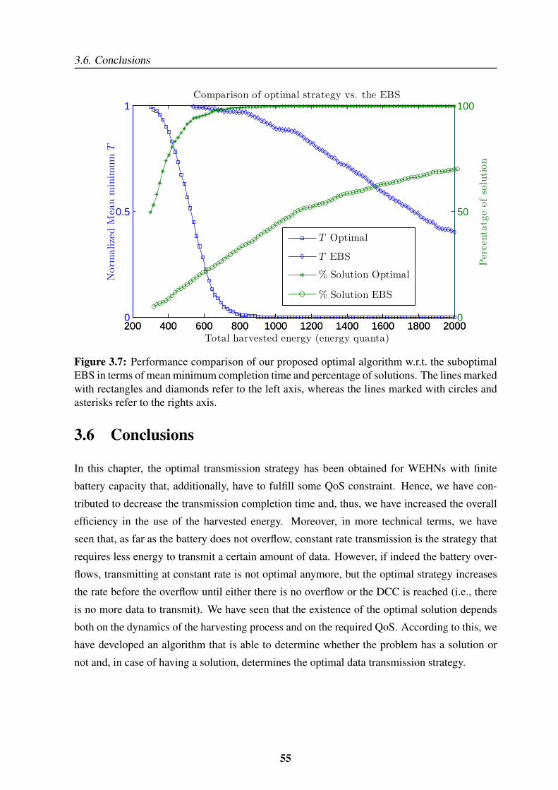
3.6. Conclusions
200 400 600 800 1000 1200 1400 1600 1800 20000
0.5
1
Total harvested energy (energy quanta)
Norm
alizedMea
nminim
um
T
Comparison of optimal strategy vs. the EBS
200 400 600 800 1000 1200 1400 1600 1800 20000
50
100
Percentatgeofsolution
T Optimal
T EBS
% Solution Optimal
% Solution EBS
Figure 3.7: Performance comparison of our proposed optimal algorithm w.r.t. the suboptimalEBS in terms of mean minimum completion time and percentage of solutions. The lines markedwith rectangles and diamonds refer to the left axis, whereas the lines marked with circles andasterisks refer to the rights axis.
3.6 Conclusions
In this chapter, the optimal transmission strategy has been obtained for WEHNs with finite
battery capacity that, additionally, have to fulfill some QoS constraint. Hence, we have con-
tributed to decrease the transmission completion time and, thus, we have increased the overall
efficiency in the use of the harvested energy. Moreover, in more technical terms, we have
seen that, as far as the battery does not overflow, constant rate transmission is the strategy that
requires less energy to transmit a certain amount of data. However, if indeed the battery over-
flows, transmitting at constant rate is not optimal anymore, but the optimal strategy increases
the rate before the overflow until either there is no overflow or the DCC is reached (i.e., there
is no more data to transmit). We have seen that the existence of the optimal solution depends
both on the dynamics of the harvesting process and on the required QoS. According to this, we
have developed an algorithm that is able to determine whether the problem has a solution or
not and, in case of having a solution, determines the optimal data transmission strategy.
55
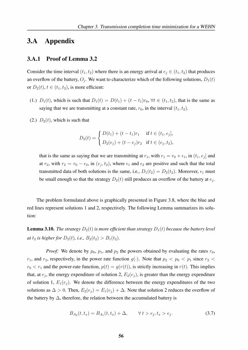
Chapter 3. Transmission completion time minimization for a WEHN
3.A Appendix
3.A.1 Proof of Lemma 3.2
Consider the time interval (t1, t2) where there is an energy arrival at ej ∈ (t1, t2) that produces
an overflow of the battery, Oj . We want to characterize which of the following solutions, D1(t)
or D2(t), t ∈ (t1, t2), is more efficient:
(1.) D1(t), which is such that D1(t) = D(t1) + (t − t1)r0, ∀t ∈ (t1, t2), that is the same as
saying that we are transmitting at a constant rate, r0, in the interval (t1, t2).
(2.) D2(t), which is such that
D2(t) =
{D(t1) + (t− t1)r1 if t ∈ (t1, ej],
D2(ej) + (t− ej)r2 if t ∈ (ej, t2),
that is the same as saying that we are transmitting at r1, with r1 = r0 + ε1, in (t1, ej] and
at r2, with r2 = r0 − ε2, in (ej, t2), where ε1 and ε2 are positive and such that the total
transmitted data of both solutions is the same, i.e., D1(t2) = D2(t2). Moreover, ε1 must
be small enough so that the strategy D2(t) still produces an overflow of the battery at ej .
The problem formulated above is graphically presented in Figure 3.8, where the blue and
red lines represent solutions 1 and 2, respectively. The following Lemma summarizes its solu-
tion:
Lemma 3.10. The strategyD2(t) is more efficient than strategyD1(t) because the battery level
at t2 is higher for D2(t), i.e., B2(t2) > B1(t2).
Proof: We denote by p0, p1, and p2 the powers obtained by evaluating the rates r0,
r1, and r2, respectively, in the power rate function g(·). Note that p2 < p0 < p1 since r2 <
r0 < r1 and the power-rate function, p(t) = g(r(t)), is strictly increasing in r(t). This implies
that, at ej , the energy expenditure of solution 2, E2(ej), is greater than the energy expenditure
of solution 1, E1(ej). We denote the difference between the energy expenditures of the two
solutions as ∆ > 0. Then, E2(ej) = E1(ej) + ∆. Note that solution 2 reduces the overflow of
the battery by ∆, therefore, the relation between the accumulated battery is
BA2(t, tx) = BA1(t, tx) + ∆, ∀ t > ej, tx > ej. (3.7)
56
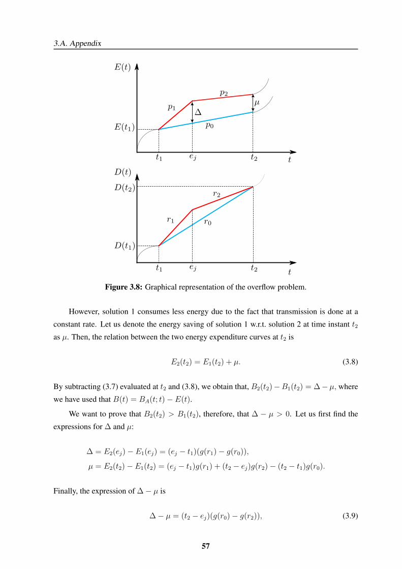
3.A. Appendix
Figure 3.8: Graphical representation of the overflow problem.
However, solution 1 consumes less energy due to the fact that transmission is done at a
constant rate. Let us denote the energy saving of solution 1 w.r.t. solution 2 at time instant t2as µ. Then, the relation between the two energy expenditure curves at t2 is
E2(t2) = E1(t2) + µ. (3.8)
By subtracting (3.7) evaluated at t2 and (3.8), we obtain that, B2(t2)−B1(t2) = ∆− µ, where
we have used that B(t) = BA(t; t)− E(t).
We want to prove that B2(t2) > B1(t2), therefore, that ∆ − µ > 0. Let us first find the
expressions for ∆ and µ:
∆ = E2(ej)− E1(ej) = (ej − t1)(g(r1)− g(r0)),
µ = E2(t2)− E1(t2) = (ej − t1)g(r1) + (t2 − ej)g(r2)− (t2 − t1)g(r0).
Finally, the expression of ∆− µ is
∆− µ = (t2 − ej)(g(r0)− g(r2)), (3.9)
57
Chapter 3. Transmission completion time minimization for a WEHN
that is greater than zero since g(r0) > g(r2).
Note that D2(t) achieves a higher battery level at t2 due to the fact that the reduction in the
battery overflow is higher than the energy saved by a constant rate transmission. Accordingly,
the optimal transmission strategy increases the rate until either there is no overflow or the data
buffer is emptied, which implies that the data departure curve must reach its upper bound, i.e.,
D(t) = DA(t). Note that the insertion of the QoS constraint, which is a lower bound on D(t),
does not affect the validity of the proof given above, which proves Lemma 3.2.
3.A.2 Rate change characterization
Proof of Lemma 3.5
The proof of the lemma is divided in two parts. We first show that if a rate change occurs at
`m, then D?(m)(`m) = D
(m)max(`−m) and, afterwards, we show that the rate must increase.
Part 1. Let us assume that a rate change occurs at `m such that D(m)(`m) < D(m)max(`−m). We
will show by contradiction that this cannot be optimal. Let us consider the time interval (`m −
ε, `m+ε) with ε being positive. Note that if we select a sufficiently small ε, we can find a straight
line with rate r = D(m)(`m+ε)−D(m)(`m−ε)2ε
, which still satisfies the constraints, that transmits the
same amount of data while having less energy expenditure. Hence, we have proved that if the
rate changes at `m, then D?(m)(`m) = D
(m)max(`−m).
Part 2. Now we prove that when the rate changes at `m, it must increase. The procedure is
the same as the one in the first part of the proof. We start by assuming that a rate decrease is
optimal and then, we see that it leads to a logical contradiction. We denote rm and rm+1 the
rates before and after `m, respectively, where rm > rm+1. We consider the same time interval.
In this case, we can also find a straight line whose slope is r = D(m)(`m+ε)−D(m)(`m−ε)2ε
, which
satisfies the energy and data constraints, that transmits the same amount of data while having
less energy expenditure. Hence, we have proved by contradiction that if the rate changes, it
must increase.
Proof of Lemma 3.6
This proof is similar to the proof of Lemma 3.5. The main difference is that now the disconti-
nuity is in the lower constraint. Then, by following the same procedure we can first show that
a rate change is suboptimal unless D?(m)(`m) = D
(m)min(`+
m) and a rate decrease is produced.
58

3.A. Appendix
Proof of Lemma 3.7
We know that `m comes from an energy arrival event, otherwise, the problem would not have
a feasible solution as stated in Lemma 3.4. This implies that D(m)max(`m) = D
(m)A (`m) and
D(m)min(`m) = D
(m)Emin
(`+m). Then, it is obvious that if D(m)
A (`m) < D(m)Emin
(`+m), an overflow is
produced. Hence, the proof that D?(m)(`m) = D
(m)max(`m) comes from Lemma 3.2, where we
show that the optimal data departure curve satisfies that when an overflow is produced, all the
data has been transmitted and, hence, the rate must change to zero until the following data
arrival.
Proof of Lemma 3.8
This lemma states that two events are produced at the time instant `m. One could look at this
lemma as the union of Lemmas 3.5 and 3.6 at the same time instant, hence, the proof has been
already given in the aforementioned lemmas.
Proof of Lemma 3.9
As we pointed out, this lemma only applies when the problem has a solution. Consequently, we
know thatD(m)min(`m) = D
(m)Emin
(`+m) and thatD(m)
max(`m) = D(m)A (`−m). Hence, this is the overflow
problem with the particularity that a data arrival is produced at `m. From Lemma 3.2, the
optimal solution minimizes the energy lost due to overflow and, thus, D?(m)(`m) = D
(m)max(`−m).
However, in this situation, nothing can be stated regarding the rate in the following pool.
3.A.3 The algorithm
In this appendix, a technical explanation of the algorithm is given. First, we introduce the
maximum and minimum rates, a concept required to understand the second and third blocks of
the algorithm that are presented afterwards.
3.A.3.1 Maximum and minimum rates
Let R(m)max denote the set that contains the rates obtained by joining the reference point, (0,
D(m)(0) = 0)8, with the discontinuities from the left ofD(m)max(t), i.e., the points (z,D
(m)max(z−)),
∀z ∈ Z(m)max, and such that the obtained curve is feasible for t ∈ (0, z), where by feasible we
mean that the curve satisfies all the constraints. Similarly, R(m)min contains the rates obtained by
8Note that the reference point is always (0, 0) as the origin of coordinates is moved at every iteration.
59
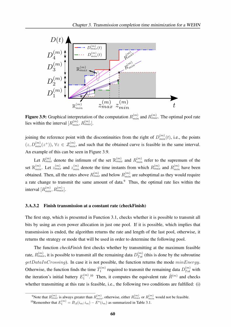
Chapter 3. Transmission completion time minimization for a WEHN
x
x
x
x
x
x
x
Figure 3.9: Graphical interpretation of the computation R(m)min and R(m)
max. The optimal pool ratelies within the interval [R
(m)min, R
(m)max].
joining the reference point with the discontinuities from the right of D(m)min(t), i.e., the points
(z,D(m)min(z+)), ∀z ∈ Z(m)
min, and such that the obtained curve is feasible in the same interval.
An example of this can be seen in Figure 3.9.
Let R(m)max denote the infimum of the set R(m)
max and R(m)min refer to the supremum of the
set R(m)min. Let z(m)
max and z(m)min denote the time instants from which R(m)
max and R(m)min have been
obtained. Then, all the rates above R(m)max and below R
(m)min are suboptimal as they would require
a rate change to transmit the same amount of data.9 Thus, the optimal rate lies within the
interval [R(m)min, R
(m)max].
3.A.3.2 Finish transmission at a constant rate (checkFinish)
The first step, which is presented in Function 3.1, checks whether it is possible to transmit all
bits by using an even power allocation in just one pool. If it is possible, which implies that
transmission is ended, the algorithm returns the rate and length of the last pool, otherwise, it
returns the strategy or mode that will be used in order to determine the following pool.
The function checkFinish first checks whether by transmitting at the maximum feasible
rate, R(m)max, it is possible to transmit all the remaining data D(m)
Tot (this is done by the subroutine
getDataInCrossing). In case it is not possible, the function returns the mode minEnergy.
Otherwise, the function finds the time T (m)1 required to transmit the remaining data D(m)
Tot with
the iteration’s initial battery E(m)1 .10 Then, it computes the equivalent rate R(m) and checks
whether transmitting at this rate is feasible, i.e., the following two conditions are fulfilled: (i)
9Note that R(m)max is always greater than R(m)
min, otherwise, either R(m)max or R(m)
min would not be feasible.10Remember that E(m)
1 = BA(im; im)− E?(im) as summarized in Table 3.1.
60
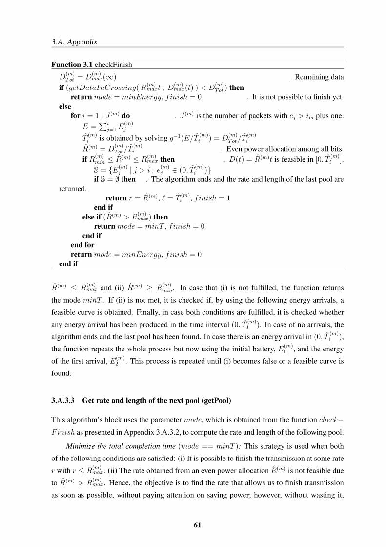
3.A. Appendix
Function 3.1 checkFinish
D(m)Tot = D
(m)max(∞) . Remaining data
if (getDataInCrossing(R(m)maxt , D
(m)max(t) ) < D
(m)Tot ) then
return mode = minEnergy, finish = 0 . It is not possible to finish yet.else
for i = 1 : J (m) do . J (m) is the number of packets with ej > im plus one.E =
∑ij=1E
(m)j
T(m)i is obtained by solving g−1(E/T
(m)i ) = D
(m)Tot/T
(m)i
R(m) = D(m)Tot/T
(m)i . Even power allocation among all bits.
if R(m)min ≤ R(m) ≤ R
(m)max then . D(t) = R(m)t is feasible in [0, T
(m)i ].
S = {E(m)j | j > i , e
(m)j ∈ (0, T
(m)i )}
if S = ∅ then . The algorithm ends and the rate and length of the last pool arereturned.
return r = R(m), ` = T(m)i , finish = 1
end ifelse if (R(m) > R
(m)max) then
return mode = minT , finish = 0end if
end forreturn mode = minEnergy, finish = 0
end if
R(m) ≤ R(m)max and (ii) R(m) ≥ R
(m)min. In case that (i) is not fulfilled, the function returns
the mode minT . If (ii) is not met, it is checked if, by using the following energy arrivals, a
feasible curve is obtained. Finally, in case both conditions are fulfilled, it is checked whether
any energy arrival has been produced in the time interval (0, T(m)1 ). In case of no arrivals, the
algorithm ends and the last pool has been found. In case there is an energy arrival in (0, T(m)1 ),
the function repeats the whole process but now using the initial battery, E(m)1 , and the energy
of the first arrival, E(m)2 . This process is repeated until (i) becomes false or a feasible curve is
found.
3.A.3.3 Get rate and length of the next pool (getPool)
This algorithm’s block uses the parameter mode, which is obtained from the function check−Finish as presented in Appendix 3.A.3.2, to compute the rate and length of the following pool.
Minimize the total completion time (mode == minT ): This strategy is used when both
of the following conditions are satisfied: (i) It is possible to finish the transmission at some rate
r with r ≤ R(m)max. (ii) The rate obtained from an even power allocation R(m) is not feasible due
to R(m) > R(m)max. Hence, the objective is to find the rate that allows us to finish transmission
as soon as possible, without paying attention on saving power; however, without wasting it,
61
Chapter 3. Transmission completion time minimization for a WEHN
either. In such case, the rate and duration of the pool are rm = R(m)max and `m = z
(m)max.
Minimize the energy expenditure (mode == minEnergy): This strategy is used when,
due to the constraints, transmission cannot be finished at a constant rate, e.g., the rate must
be increased to satisfy the QoS constraints. Hence, the objective is to save as much energy as
possible in order to use it when ending the transmission is feasible. Note that in this situation,
the problem of obtaining the following pool is similar to the problem presented in [55] and,
hence, the solution is also similar. The possible data departure curves with constant rate r, i.e.,
D(m)(t) = rt, are divided in two sets. The first set S(m)Rmax
contains all the rates r such that
the associated data departure curve crosses the constraint D(m)max(t) first. Whereas the set S(m)
Rmin
contains all the rates r such that the associated data departure curve crosses the constraint
D(m)min(t) first. Then, the rate of the following pool is determined as the infimum of S(m)
Rmax
or, equivalently, the supremum of S(m)Rmin
, i.e., rm = inf(S(m)Rmax
)= sup
(S(m)Rmin
)and the
duration of the pool `m can be obtained as the first time instant such that, rm`m = D(m)max(`m)
or rm`m = D(m)min(`m).
3.A.3.4 Proof of the algorithm optimality
At each iteration, the algorithm checks whether Lemma 3.4 is fulfilled. In such a case, there
is no solution for the problem and the algorithm ends. Otherwise, the algorithm must satisfy
Lemmas 3.5-3.9 at each rate change and Lemma 3.3 by the end of the transmission. To show
that these lemmas are satisfied and, hence, the algorithm computes the optimal data departure
curve, we focus on the three different situations that can occur depending on the constraints
of the problem: (i) The algorithm finishes transmission by using an even power allocation
among all bits to be transmitted. (ii) minT strategy is used to obtain the pool. (iii) The pool is
computed by usingminEnergy mode. In the following, the optimality of these cases is proved
by showing that the algorithm-chosen solution satisfies the optimality conditions and that it is
unique.
Part 1 (Even power allocation). When this situation occurs, the algorithm ends transmission by
transmitting at a constant rate. Hence, Lemma 3.1 is satisfied. No overflow is produced, thus,
Lemma 3.2 is satisfied. Lemmas from 3.5 to 3.9 do not apply since there are no rate changes.
Finally, note that Lemma 3.3 is satisfied, since the last rate rM is obtained as the rate that allows
the transmission of all the data by using all the available energy, moreover, from the properties
of the function g(·) this rate is unique.
Part 2 (minT mode). We want to demonstrate that the optimal departure curve transmits at
R(m)max during a period of time z(m)
max. Let T (m) be the total completion time that would be
62

3.A. Appendix
obtained if transmitting at rate R(m) was feasible, hence, T (m) = D(m)Tot/R
(m). Similarly,
T(m)max = D
(m)Tot/R
(m)max. Note that, since R(m)
max is a feasible rate, T (m)max is an upper bound of
the remaining completion time, T (m), whereas T (m) is a lower bound, hence:
T (m) < T (m) < T (m)max. (3.10)
Consider the data departure curve D(m)1 (t) = R
(m)maxt. Note that any other data departure
curve, D(m)2 (t), is suboptimal since, in order to satisfy (3.10), D(m)
2 (t) will cross D(m)1 (t) for
some ty ∈ (0, T(m)max). Hence, at ty, both curves have sent the same amount of data; however,
D(m)1 (t) has consumed less energy.
Now we must show that, at z(m)max, the rate increases. Note that by transmitting at R(m)
max
instead of at R(m), some energy has been saved. Then, in the following pool, the available
energy per bit is higher and, then, the new rate R(m+1) obtained from an even power allocation
among all bits in the following pool fulfills R(m+1) > R(m) > R(m)max. Hence, we have proved
that at z(m)max a rate increase is produced.
Part 3 (minEnergy mode). This mode is used when it is not possible to finish transmission
at any rate. Note that the algorithm can select three different kind of points, denoted as vx =
(`m, D?(m)
(`m)), for ending the pool depending on the constraints:
• v1 |D?(m)(`m) = D
(m)max(`−m) where `m is either d(m)
i or e(m)j .
• v2 |D?(m)(`m) = D
(m)min(`+
m) where `m is either q(m)k or e(m)
j .
• v3 |D?(m)(`m) = D
(m)max(`−m) where `m is e(m)
j and an overflow is produced.
Note that Corollary 3.1 and Lemma 3.2 are satisfied for any of the selected points and that
Lemma 3.3 does not apply since transmission cannot be ended yet. Hence, we have to prove
the following three conditions: (i) If a point such as v1 is selected, there will be a rate increase
(Lemma 3.5 or Lemma 3.8 for the case that at `m two events are produced). (ii) If a point such
as v2 is selected, there will be a rate decrease (Lemma 3.6 or Lemma 3.8 for the case that at `m
two events are produced). And (iii), if a point such as v3 is selected, the rate of the following
pool is zero as far as `3 is not a data arrival event (Lemma 3.7 and Lemma 3.9).
Regarding (i), the rate of the pool is rm = D(m)max(`−m)`m
that is the supremum of S(m)Rmin
. Note
that, at the following iteration, the set S(m+1)Rmin
includes all the rates in the interval (0, rm) and
63

Chapter 3. Transmission completion time minimization for a WEHN
the rates contained in the interval (rm, rm+ ε), for some ε > 0. Hence, the rate of the following
iteration, rm+1, satisfies that rm+1 ≥ rm, therefore, a rate increase is produced. A similar
approach can be done for (ii), the rate of the pool is rm =D
(m)min(`+m)
`mthat is the infimum of
S(m)Rmax
. At the following iteration the set S(m+1)Rmax
contains all the rates in (rm − ε,∞) for some
ε > 0. Hence, the rate of the following iteration, rm+1, satisfies that rm+1 ≤ rm and, therefore,
there is a rate decrease. Finally, in case (iii), an overflow of the battery is produced. Note
that the solution chosen by the algorithm satisfies that all the available data at `−3 has been
transmitted. This implies that if non-data arrival is produced at `3 the rate of the following pool
must be zero in order to satisfy the DCC.
Therefore, the algorithm computes the optimal solution since it satisfies all the lemmas
that model the behavior of the optimal solution.
64
Chapter 4On the precoder design of a wireless energy
harvesting node in linear vector Gaussian
channels with arbitrary input distribution
4.1 Introduction
In the previous chapter, we have studied a scenario where data dynamically arrives to the trans-
mitter and thoroughly examined the effect of the DCCs and the finite buffer constraint over the
optimal continuous-time transmission strategy. In opposition, the remaining chapters of this
dissertation, consider the scenario in which the node has an infinite backlog of data to be trans-
mitted through a discrete-time memoryless channel. Accordingly, in the remaining chapters,
we aim to design transmission strategies that transmit the maximum amount of data by using
the harvested energy.
Since the transmitter has always data to be transmitted, the DCCs are trivially satisfied and
it is known that battery overflows are suboptimal. Thus, one can impose that the transmission
strategy does not produce any battery overflows by imposing an additional set of constraints to
the problem. Given a generic power consumption model C(·) and the packetized model of the
energy harvesting process in Figure 2.13, the ECCs and the finite battery capacity constraints
can be written as
Ts∑`
j=1
∑n∈τj C(pn) ≤
∑`j=1Ej, ` = 1, . . . , J, (4.1)
and∑`
j=1Ej −∑`−1
j=1 Ts∑
n∈τj C(pn) ≤ Cmax, ` = 2, . . . , J, (4.2)
65
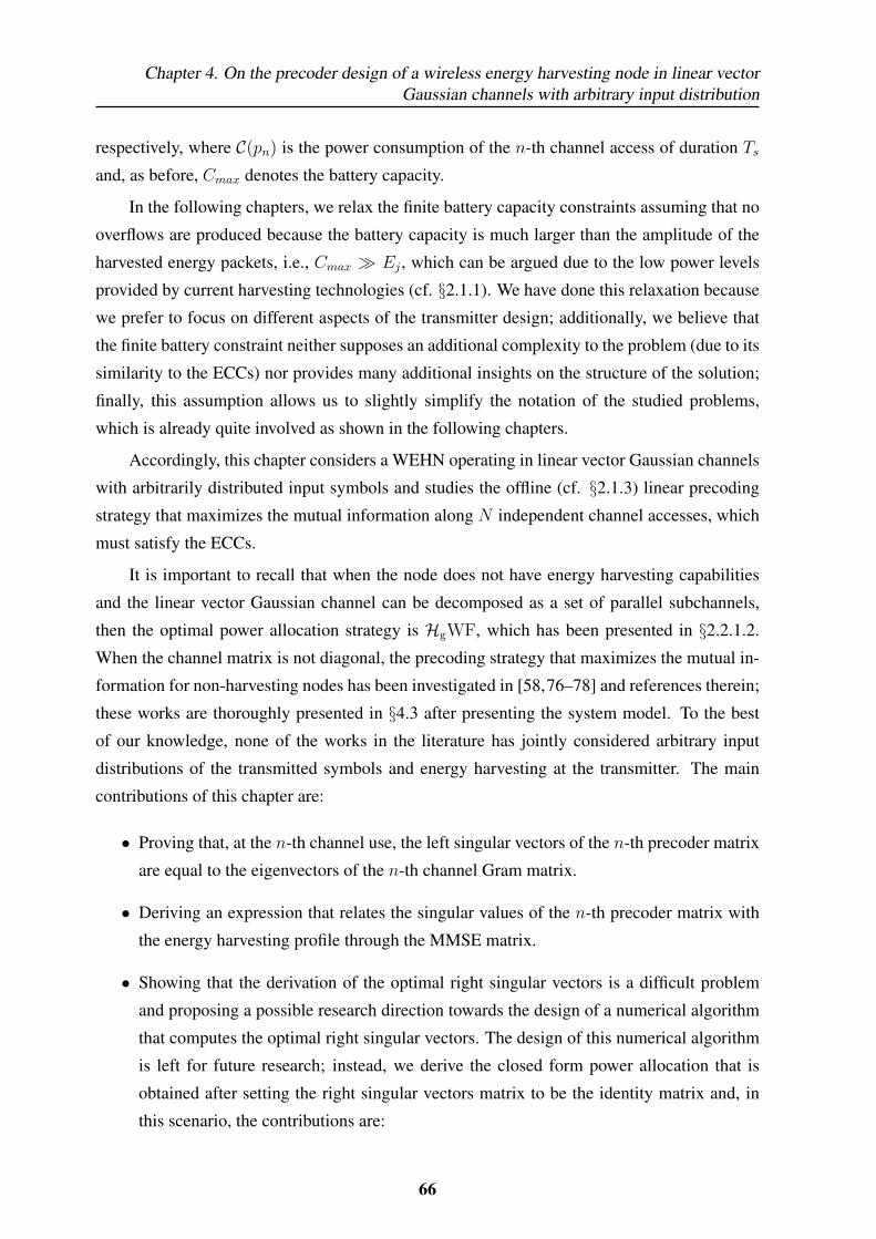
Chapter 4. On the precoder design of a wireless energy harvesting node in linear vectorGaussian channels with arbitrary input distribution
respectively, where C(pn) is the power consumption of the n-th channel access of duration Tsand, as before, Cmax denotes the battery capacity.
In the following chapters, we relax the finite battery capacity constraints assuming that no
overflows are produced because the battery capacity is much larger than the amplitude of the
harvested energy packets, i.e., Cmax � Ej , which can be argued due to the low power levels
provided by current harvesting technologies (cf. §2.1.1). We have done this relaxation because
we prefer to focus on different aspects of the transmitter design; additionally, we believe that
the finite battery constraint neither supposes an additional complexity to the problem (due to its
similarity to the ECCs) nor provides many additional insights on the structure of the solution;
finally, this assumption allows us to slightly simplify the notation of the studied problems,
which is already quite involved as shown in the following chapters.
Accordingly, this chapter considers a WEHN operating in linear vector Gaussian channels
with arbitrarily distributed input symbols and studies the offline (cf. §2.1.3) linear precoding
strategy that maximizes the mutual information along N independent channel accesses, which
must satisfy the ECCs.
It is important to recall that when the node does not have energy harvesting capabilities
and the linear vector Gaussian channel can be decomposed as a set of parallel subchannels,
then the optimal power allocation strategy is HgWF, which has been presented in §2.2.1.2.
When the channel matrix is not diagonal, the precoding strategy that maximizes the mutual in-
formation for non-harvesting nodes has been investigated in [58,76–78] and references therein;
these works are thoroughly presented in §4.3 after presenting the system model. To the best
of our knowledge, none of the works in the literature has jointly considered arbitrary input
distributions of the transmitted symbols and energy harvesting at the transmitter. The main
contributions of this chapter are:
• Proving that, at the n-th channel use, the left singular vectors of the n-th precoder matrix
are equal to the eigenvectors of the n-th channel Gram matrix.
• Deriving an expression that relates the singular values of the n-th precoder matrix with
the energy harvesting profile through the MMSE matrix.
• Showing that the derivation of the optimal right singular vectors is a difficult problem
and proposing a possible research direction towards the design of a numerical algorithm
that computes the optimal right singular vectors. The design of this numerical algorithm
is left for future research; instead, we derive the closed form power allocation that is
obtained after setting the right singular vectors matrix to be the identity matrix and, in
this scenario, the contributions are:
66
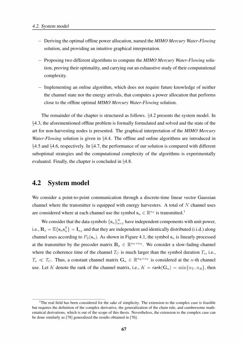
4.2. System model
− Deriving the optimal offline power allocation, named the MIMO Mercury Water-Flowing
solution, and providing an intuitive graphical interpretation.
− Proposing two different algorithms to compute the MIMO Mercury Water-Flowing solu-
tion, proving their optimality, and carrying out an exhaustive study of their computational
complexity.
− Implementing an online algorithm, which does not require future knowledge of neither
the channel state nor the energy arrivals, that computes a power allocation that performs
close to the offline optimal MIMO Mercury Water-Flowing solution.
The remainder of the chapter is structured as follows. §4.2 presents the system model. In
§4.3, the aforementioned offline problem is formally formulated and solved and the state of the
art for non-harvesting nodes is presented. The graphical interpretation of the MIMO Mercury
Water-Flowing solution is given in §4.4. The offline and online algorithms are introduced in
§4.5 and §4.6, respectively. In §4.7, the performance of our solution is compared with different
suboptimal strategies and the computational complexity of the algorithms is experimentally
evaluated. Finally, the chapter is concluded in §4.8.
4.2 System model
We consider a point-to-point communication through a discrete-time linear vector Gaussian
channel where the transmitter is equipped with energy harvesters. A total of N channel uses
are considered where at each channel use the symbol sn ∈ RnS is transmitted.1
We consider that the data symbols {sn}Nn=1 have independent components with unit power,
i.e., Rs = E{snsTn} = InS and that they are independent and identically distributed (i.i.d.) along
channel uses according to PS(sn). As shown in Figure 4.1, the symbol sn is linearly processed
at the transmitter by the precoder matrix Bn ∈ RnT×nS . We consider a slow-fading channel
where the coherence time of the channel TC is much larger than the symbol duration Ts, i.e.,
Ts � TC . Thus, a constant channel matrix Gn ∈ RnR×nT is considered at the n-th channel
use. Let K denote the rank of the channel matrix, i.e., K = rank(Gn) = min{nT , nR}, then
1The real field has been considered for the sake of simplicity. The extension to the complex case is feasiblebut requires the definition of the complex derivative, the generalization of the chain rule, and cumbersome math-ematical derivations, which is out of the scope of this thesis. Nevertheless, the extension to the complex case canbe done similarly as [78] generalized the results obtained in [76].
67
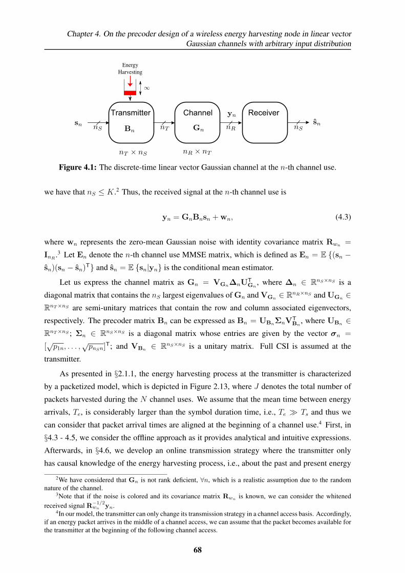
Chapter 4. On the precoder design of a wireless energy harvesting node in linear vectorGaussian channels with arbitrary input distribution
Transmitter Channel Receiver
Figure 4.1: The discrete-time linear vector Gaussian channel at the n-th channel use.
we have that nS ≤ K.2 Thus, the received signal at the n-th channel use is
yn = GnBnsn + wn, (4.3)
where wn represents the zero-mean Gaussian noise with identity covariance matrix Rwn =
InR .3 Let En denote the n-th channel use MMSE matrix, which is defined as En = E {(sn −sn)(sn − sn)T} and sn = E {sn|yn} is the conditional mean estimator.
Let us express the channel matrix as Gn = VGn∆nUTGn
, where ∆n ∈ RnS×nS is a
diagonal matrix that contains the nS largest eigenvalues of Gn and VGn ∈ RnR×nS and UGn ∈RnT×nS are semi-unitary matrices that contain the row and column associated eigenvectors,
respectively. The precoder matrix Bn can be expressed as Bn = UBnΣnVTBn
, where UBn ∈RnT×nS ; Σn ∈ RnS×nS is a diagonal matrix whose entries are given by the vector σn =
[√p1n, . . . ,
√pnSn]T; and VBn ∈ RnS×nS is a unitary matrix. Full CSI is assumed at the
transmitter.
As presented in §2.1.1, the energy harvesting process at the transmitter is characterized
by a packetized model, which is depicted in Figure 2.13, where J denotes the total number of
packets harvested during the N channel uses. We assume that the mean time between energy
arrivals, Te, is considerably larger than the symbol duration time, i.e., Te � Ts and thus we
can consider that packet arrival times are aligned at the beginning of a channel use.4 First, in
§4.3 - 4.5, we consider the offline approach as it provides analytical and intuitive expressions.
Afterwards, in §4.6, we develop an online transmission strategy where the transmitter only
has causal knowledge of the energy harvesting process, i.e., about the past and present energy
2We have considered that Gn is not rank deficient, ∀n, which is a realistic assumption due to the randomnature of the channel.
3Note that if the noise is colored and its covariance matrix Rwn is known, we can consider the whitenedreceived signal R
−1/2wn yn.
4In our model, the transmitter can only change its transmission strategy in a channel access basis. Accordingly,if an energy packet arrives in the middle of a channel access, we can assume that the packet becomes available forthe transmitter at the beginning of the following channel access.
68
4.3. Throughput maximization problem
arrivals (cf. §2.1.3). Recall that, as presented in §2.1.1, we use the term epoch, τj, j = 1, . . . , J ,
to denote the set of channel accesses between two consecutive energy arrivals. As argued at the
beginning of the chapter, we assume an infinite capacity battery.
4.3 Throughput maximization problem
In this section, we study the set of linear precoding matrices {Bn}Nn=1 that maximizes the input-
output mutual information along N independent channel accesses,∑J
j=1
∑n∈τj I(sn; yn),
where I(sn; yn) is the n-th channel use mutual information. The design of {Bn}Nn=1 is con-
strained to satisfy the instantaneous ECCs, which impose that energy cannot be used before it
has been harvested, Ts∑`
j=1
∑n∈τj ||Bnsn||2 ≤
∑`j=1Ej , ` = 1, . . . , J . However, since in
each epoch there are several channel accesses with the same channel gains (because Tc � Ts
and Te � Ts), instead of imposing the instantaneous ECCs, we can consider the mean ECCs
that become Ts∑`
j=1
∑n∈τj Tr(BnB
Tn) ≤
∑`j=1 Ej , ` = 1, . . . , J , which do not require prior
knowledge of the transmitted symbols at each channel use as only the expectation of the sym-
bols is needed.5
Therefore, the mutual information maximization problem is mathematically expressed as
maximize{Bn}Nn=1
J∑j=1
∑n∈τj
I(sn; yn) (4.4a)
subject to Ts∑j=1
∑n∈τj
Tr(BnBTn) ≤
∑j=1
Ej, ` = 1, . . . , J. (4.4b)
Before addressing the problem in (4.4), let us summarize the state of the art on the pre-
coding strategy that maximizes the mutual information for non-harvesting nodes, which was
studied in [58, 76–78] and references therein.6 In [58], it was shown that, in general, the mu-
tual information, I(sn; yn), is not a concave function of the precoder and that depends on the
precoder only through the matrix Zn = BTnGT
nGnBn. The authors of [58] also showed that the
left singular vectors of the precoder can be chosen to be equal to the eigenvectors of the channel
5In general, the energy harvesting and the channel state are two independent random processes. Thus, theremay be situations in which only a few channel accesses separate an energy arrival from a change in the channelrealization; however, note that these situations are unlikely since Tc � Ts and Te � Ts. In these unlikelysituations, the temporal averaging is not sufficient to ensure that the fulfillment of the mean ECCs implies afulfillment of the instantaneous ECCs; however, the averaging through the different channel dimensions bringscloser the mean and instantaneous ECCs. Thus, the mean ECCs can be used instead of the instantaneous ECCssince the cases in which they differ are indeed very unlikely.
6When there is no energy harvesting at the transmitter, the mutual information maximization problem is theone obtained after setting J = 1 and N = 1 in (4.4). Thus, the mutual information is maximized for a singlechannel use under a power constraint.
69
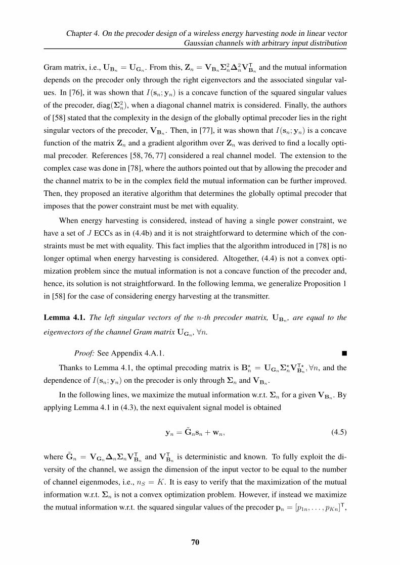
Chapter 4. On the precoder design of a wireless energy harvesting node in linear vectorGaussian channels with arbitrary input distribution
Gram matrix, i.e., UBn = UGn . From this, Zn = VBnΣ2n∆
2nV
TBn
and the mutual information
depends on the precoder only through the right eigenvectors and the associated singular val-
ues. In [76], it was shown that I(sn; yn) is a concave function of the squared singular values
of the precoder, diag(Σ2n), when a diagonal channel matrix is considered. Finally, the authors
of [58] stated that the complexity in the design of the globally optimal precoder lies in the right
singular vectors of the precoder, VBn . Then, in [77], it was shown that I(sn; yn) is a concave
function of the matrix Zn and a gradient algorithm over Zn was derived to find a locally opti-
mal precoder. References [58, 76, 77] considered a real channel model. The extension to the
complex case was done in [78], where the authors pointed out that by allowing the precoder and
the channel matrix to be in the complex field the mutual information can be further improved.
Then, they proposed an iterative algorithm that determines the globally optimal precoder that
imposes that the power constraint must be met with equality.
When energy harvesting is considered, instead of having a single power constraint, we
have a set of J ECCs as in (4.4b) and it is not straightforward to determine which of the con-
straints must be met with equality. This fact implies that the algorithm introduced in [78] is no
longer optimal when energy harvesting is considered. Altogether, (4.4) is not a convex opti-
mization problem since the mutual information is not a concave function of the precoder and,
hence, its solution is not straightforward. In the following lemma, we generalize Proposition 1
in [58] for the case of considering energy harvesting at the transmitter.
Lemma 4.1. The left singular vectors of the n-th precoder matrix, UBn , are equal to the
eigenvectors of the channel Gram matrix UGn , ∀n.
Proof: See Appendix 4.A.1.
Thanks to Lemma 4.1, the optimal precoding matrix is B?n = UGnΣ
?nV
T?Bn,∀n, and the
dependence of I(sn; yn) on the precoder is only through Σn and VBn .
In the following lines, we maximize the mutual information w.r.t. Σn for a given VBn . By
applying Lemma 4.1 in (4.3), the next equivalent signal model is obtained
yn = Gnsn + wn, (4.5)
where Gn = VGn∆nΣnVTBn
and VTBn
is deterministic and known. To fully exploit the di-
versity of the channel, we assign the dimension of the input vector to be equal to the number
of channel eigenmodes, i.e., nS = K. It is easy to verify that the maximization of the mutual
information w.r.t. Σn is not a convex optimization problem. However, if instead we maximize
the mutual information w.r.t. the squared singular values of the precoder pn = [p1n, . . . , pKn]T,
70
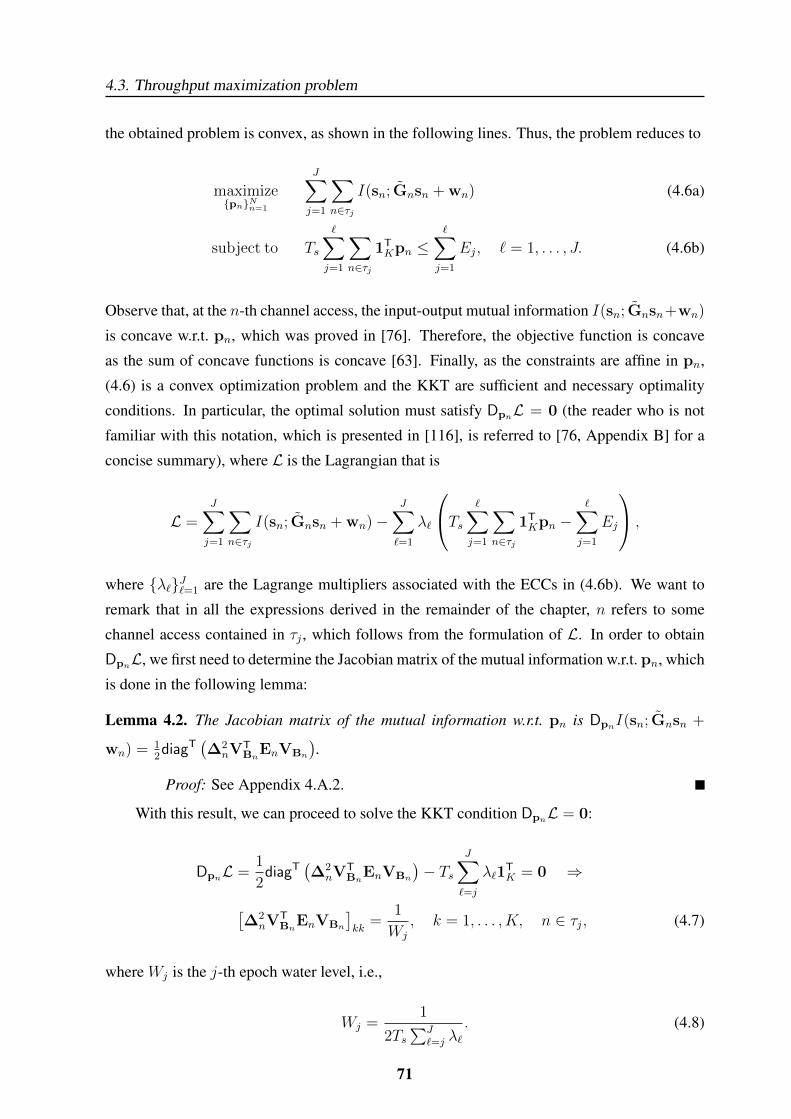
4.3. Throughput maximization problem
the obtained problem is convex, as shown in the following lines. Thus, the problem reduces to
maximize{pn}Nn=1
J∑j=1
∑n∈τj
I(sn; Gnsn + wn) (4.6a)
subject to Ts∑j=1
∑n∈τj
1TKpn ≤
∑j=1
Ej, ` = 1, . . . , J. (4.6b)
Observe that, at the n-th channel access, the input-output mutual information I(sn; Gnsn+wn)
is concave w.r.t. pn, which was proved in [76]. Therefore, the objective function is concave
as the sum of concave functions is concave [63]. Finally, as the constraints are affine in pn,
(4.6) is a convex optimization problem and the KKT are sufficient and necessary optimality
conditions. In particular, the optimal solution must satisfy DpnL = 0 (the reader who is not
familiar with this notation, which is presented in [116], is referred to [76, Appendix B] for a
concise summary), where L is the Lagrangian that is
L =J∑j=1
∑n∈τj
I(sn; Gnsn + wn)−J∑`=1
λ`
Ts∑j=1
∑n∈τj
1TKpn −
∑j=1
Ej
,
where {λ`}J`=1 are the Lagrange multipliers associated with the ECCs in (4.6b). We want to
remark that in all the expressions derived in the remainder of the chapter, n refers to some
channel access contained in τj , which follows from the formulation of L. In order to obtain
DpnL, we first need to determine the Jacobian matrix of the mutual information w.r.t. pn, which
is done in the following lemma:
Lemma 4.2. The Jacobian matrix of the mutual information w.r.t. pn is DpnI(sn; Gnsn +
wn) = 12diagT
(∆2
nVTBn
EnVBn
).
Proof: See Appendix 4.A.2.
With this result, we can proceed to solve the KKT condition DpnL = 0:
DpnL =1
2diagT
(∆2
nVTBn
EnVBn
)− Ts
J∑`=j
λ`1TK = 0 ⇒
[∆2
nVTBn
EnVBn
]kk
=1
Wj
, k = 1, . . . , K, n ∈ τj, (4.7)
where Wj is the j-th epoch water level, i.e.,
Wj =1
2Ts∑J
`=j λ`. (4.8)
71

Chapter 4. On the precoder design of a wireless energy harvesting node in linear vectorGaussian channels with arbitrary input distribution
From (4.7), at each channel use, we obtain a set ofK conditions that relate the power allocation
in each stream (through the MMSE matrix) with the energy harvesting profile (through the
epoch’s water level). Some properties of the water level Wj can be derived from the KKT
optimality conditions:
λ` ≥ 0, ∀`, (4.9)
λ`
Ts∑j=1
∑n∈τj
1TKpn −
∑j=1
Ej
= 0, ∀`. (4.10)
Plugging (4.9) in (4.8), it is straightforward to obtain the following property:
Property 4.1. The water level is non-decreasing in time.7
From (4.10), we can get more insights in the solution. There are two possibilities to fulfill
(4.10):
• Empty battery: This situation occurs when, at the end of the `-th epoch, the node has
consumed all the energy, i.e., Ts∑`
j=1
∑n∈τj 1T
Kpn −∑`
j=1 Ej = 0.
• Energy flow: This situation occurs when, at the end of the `-th epoch, the node has some
remaining energy in the battery, which will be used in the following epochs. When this
happens λ` = 0 and, hence, W`+1 = W`.
Property 4.2. Changes on the water level are only produced when at the end of the previous
epoch the node has consumed all the available energy.
Note that the ECCs take into account the energy spent by the node over all the dimensions.
Thus, these two properties also hold in a scalar channel model as proved in [85, Theorem 3].
Since the problem in (4.6) is convex, by using (4.7) and Properties 4.1 and 4.2, we can
construct efficient numerical algorithms to compute the optimal power allocation, {p?n}Nn=1,
for a given VBn . The maximization of the mutual information w.r.t. VBn is indeed much
more complicated as pointed out in [58] for the non-harvesting scenario. In this context, in
this work, we focus on the particular case in which VBn = IK because, in spite of not being
necessarily the globally optimal precoder, it leads to an analytical closed form power allocation
that allows an intuitive graphical representation of the solution, as it is explained in the next
section. Observe that for any other choice VBn 6= IK , we must resort to numerical methods to
compute the optimal power allocation.
7This property is only valid under an infinity battery capacity assumption. When a finite battery is consideredthe water level may increase or decrease [84].
72

4.4. The MIMO Mercury Water-Flowing solution
The design and development of a numerical algorithm that computed the globally optimal
precoder at each channel access would be an interesting research problem in its own and is left
for future research. We believe that a possible starting point would be to analyze how to expand
the algorithms presented in [77] and [78], which exploit the concavity of the mutual informa-
tion w.r.t. the matrix Zn and the fact that the power constraint must be met with equality, to
the energy harvesting scenario. Note that if we knew the optimal total power allocation in each
channel access, we could run N times the algorithm proposed in [78] to obtain the globally
optimal precoder in each channel access; however, this approach has two major drawbacks.
First, the optimal total power allocation in each channel access is not known a priori and its
computation is not straightforward since the total power consumptions of the different channel
accesses belonging to the same epoch must simultaneously satisfy (4.7). The second drawback
is the required computational burden since any iterative approach requires a new estimation of
the MMSE matrix, En, at every iteration since it depends on VBn and Σn. These two reasons
make challenging the applicability of the proposed approach and, hence, different alternatives
to find the globally optimal precoder may be required. Altogether, we believe that the develop-
ment of a numerical algorithm that computes the globally optimal precoder for a WEHN is the
object of a new work in its own and is left for future research.
4.4 The MIMO Mercury Water-Flowing solution
In the remainder of the chapter, we consider a communication system in which the precoder is
constrained to satisfy VBn = IK or, equivalently, a communication system such that both the
precoder and channel matrices are diagonal. In spite of the fact that the total achievable mutual
information is reduced by forcing VBn = IK , we consider that it is interesting to study this
scenario for the following three reasons:
• The system y′n = ∆nΣnsn + w′n, with w′n being the observed noise at the receiver, is
commonly encountered in practical systems where, for simplicity at the decoder, inde-
pendent symbols are transmitted in each dimension (e.g., in multi-tone transmissions like
OFDM), and it has been broadly considered in the literature, indeed, theHgWF solution
was derived for such an input-output system model in [57].
• The optimal power allocation, which is named Mercury Water-Flowing, accepts a closed
form expression and an intuitive graphical representation.
• We believe that the intuition gained thanks to the Mercury Water-Flowing graphical in-
terpretation may help for the design of the algorithm that computes the globally optimal
precoder of the problem in (4.4).
73
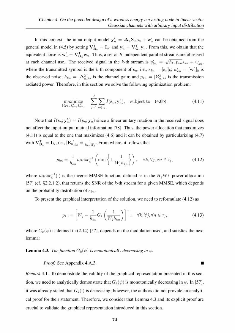
Chapter 4. On the precoder design of a wireless energy harvesting node in linear vectorGaussian channels with arbitrary input distribution
In this context, the input-output model y′n = ∆nΣnsn + w′n can be obtained from the
general model in (4.5) by setting VTBn
= IK and y′n = VTGn
yn. From this, we obtain that the
equivalent noise is w′n = VTGn
wn. Thus, a set of K independent parallel streams are observed
at each channel use. The received signal in the k-th stream is y′kn =√hknpknskn + w′kn,
where the transmitted symbol is the k-th component of sn, i.e., skn = [sn]k; w′kn = [w′n]k is
the observed noise; hkn = [∆2n]kk is the channel gain; and pkn = [Σ2
n]kk is the transmission
radiated power. Therefore, in this section we solve the following optimization problem:
maximize{{pkn}Kk=1}
Nn=1
J∑j=1
∑n∈τj
I(sn; y′n), subject to (4.6b). (4.11)
Note that I(sn; y′n) = I(sn; yn) since a linear unitary rotation in the received signal does
not affect the input-output mutual information [78]. Thus, the power allocation that maximizes
(4.11) is equal to the one that maximizes (4.6) and it can be obtained by particularizing (4.7)
with VTBn
= IK , i.e., [En]kk = 1hknWj
. From where, it follows that
pkn =1
hknmmse−1
k
(min
{1,
1
Wjhkn
}), ∀k,∀j,∀n ∈ τj, (4.12)
where mmse−1k (·) is the inverse MMSE function, defined as in the HgWF power allocation
[57] (cf. §2.2.1.2), that returns the SNR of the k-th stream for a given MMSE, which depends
on the probability distribution of skn.
To present the graphical interpretation of the solution, we need to reformulate (4.12) as
pkn =
[Wj −
1
hknGk
(1
Wjhkn
)]+
, ∀k,∀j,∀n ∈ τj, (4.13)
where Gk(ψ) is defined in (2.14) [57], depends on the modulation used, and satisfies the next
lemma:
Lemma 4.3. The function Gk(ψ) is monotonically decreasing in ψ.
Proof: See Appendix 4.A.3.
Remark 4.1. To demonstrate the validity of the graphical representation presented in this sec-
tion, we need to analytically demonstrate that Gk(ψ) is monotonically decreasing in ψ. In [57],
it was already stated that Gk(·) is decreasing; however, the authors did not provide an analyti-
cal proof for their statement. Therefore, we consider that Lemma 4.3 and its explicit proof are
crucial to validate the graphical representation introduced in this section.
74

4.4. The MIMO Mercury Water-Flowing solution
Observe the similarity of the power allocation found in (4.13) with the HgWF in (2.13)
[57]. The main difference of our solution is that, due to the nature of the energy harvesting
process, the water level depends on the channel access. Indeed, from Properties 4.1 and 4.2 we
have seen that the node is able to increase the water level as energy is being harvested.
Moreover, observe that if we particularize (4.13) for Gaussian distributed inputs, which
have Gk(ψ) = 1, ∀ψ, (see [57]), the DWF solution in (2.21) (cf. §2.3.1) is recovered. There-
fore, the mercury factor gives a measure of how the power allocation is modified when using
non-Gaussian input distributions.
LetH{kn}g (Wj) be the mercury level of the k-th stream at the n-th channel use, i.e.,
H{kn}g (Wj) =1
hknGk
(1
Wjhkn
), ∀k,∀j,∀n ∈ τj, (4.14)
which depends on the gain and water level of the channel use. Then, the power allocated in a
certain stream is the difference between the water and mercury levels, i.e.,
pkn =[Wj −H{kn}g (Wj)
]+.
The solution interpretation presented in this section is based on the fact that the mercury level
is monotonically increasing in Wj , which follows directly from Lemma 4.3, and generalizes
both theHgWF and the DWF solutions derived in [57] and [84], respectively, which have been
presented in §2.2.1.2 and §2.3.1. The MIMO Mercury Water-Flowing interpretation, depicted
in Figure 4.2, is the following:
(1.) Each parallel channel is represented with a water-porous mercury-nonporous vessel with
a base of area Ts8.
(2.) Then, each vessel is filled with a solid substance up to a height equal to h−1kn .
(3.) A water right-permeable material is used to separate the different epochs.
(4.) Each vessel has a faucet that controls the rhythm at which mercury is poured. The faucet
modifies the mercury flow so that the relation between mercury and water levels in (4.14)
is always satisfied.
(5.) Simultaneously,
• The water level is progressively increased to all epochs at the same time, adding the
necessary amount of water to each epoch. The maximum amount of water that can
8The vessel boundaries are not depicted in Figure 4.2 for the sake of simplicity.
75
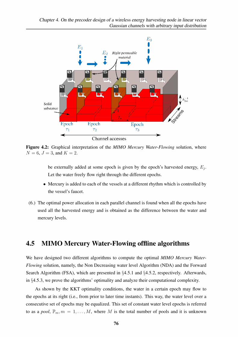
Chapter 4. On the precoder design of a wireless energy harvesting node in linear vectorGaussian channels with arbitrary input distribution
Figure 4.2: Graphical interpretation of the MIMO Mercury Water-Flowing solution, whereN = 6, J = 3, and K = 2.
be externally added at some epoch is given by the epoch’s harvested energy, Ej .
Let the water freely flow right through the different epochs.
• Mercury is added to each of the vessels at a different rhythm which is controlled by
the vessel’s faucet.
(6.) The optimal power allocation in each parallel channel is found when all the epochs have
used all the harvested energy and is obtained as the difference between the water and
mercury levels.
4.5 MIMO Mercury Water-Flowing offline algorithms
We have designed two different algorithms to compute the optimal MIMO Mercury Water-
Flowing solution, namely, the Non Decreasing water level Algorithm (NDA) and the Forward
Search Algorithm (FSA), which are presented in §4.5.1 and §4.5.2, respectively. Afterwards,
in §4.5.3, we prove the algorithms’ optimality and analyze their computational complexity.
As shown by the KKT optimality conditions, the water in a certain epoch may flow to
the epochs at its right (i.e., from prior to later time instants). This way, the water level over a
consecutive set of epochs may be equalized. This set of constant water level epochs is referred
to as a pool, Pm,m = 1, . . . ,M , where M is the total number of pools and it is unknown
76

4.5. MIMO Mercury Water-Flowing offline algorithms
a priori.9 Note that, since the epochs are a partition of the pools, a certain epoch τj is only
contained in one pool. However, a pool may contain several epochs, therefore, M ≤ J .
To compute the power allocation in (4.13), we just need to determine which epochs are
contained in each pool Pm as, once the pools are known, the optimal power allocation of the
pool can be found by performing the Mercury/Water-Filling Algorithm (HgWFA) introduced
in [57], where the m-th pool water level, Wm, is found by forcing that the energy expended in
the pool has to be equal to the energy harvested, which follows from Property 4.2.
The following two algorithms use a different approach two determine the pools:
4.5.1 NDA
The NDA uses the fact that a water level decrease is suboptimal, which follows from the KKT
conditions (see Property 4.1), to compute the optimal power allocation as follows:
(1.) Initially, set M := J , i.e., every pool contains one epoch Pm := {τm}, m = 1, . . . ,M.
(2.) Perform theHgWFA in [57] to every pool to obtain the water level, Wm, in each pool.
(3.) Look for some pool, m′, at which the water level decreases, i.e., Wm′ > Wm′+1:
• If some pool is found, merge this pool with the following pool, i.e., Pm′ := Pm′ ∪Pm′+1. The harvested energy of the resulting pool is the sum of the two original
pools. Then, the total number of pools has been reduced by one, i.e., M := M − 1.
Perform theHgWFA to obtain the new water level of the m′-th pool, i.e., Wm′ , and
go back to 3.
• If no pool is found, the optimal M has been found along with the optimal power
allocation.
4.5.2 FSA
The FSA determines the different pools by finding the optimal transition epochs, {T ?m}Mm=1,
that are defined as the first epoch of each pool. As stated before, once the pools are known the
optimal power allocation is determined by applying the HgWFA to each pool.10 To determine
{T ?m}Mm=1, we have designed a forward-search algorithm that extends the algorithm introduced
9In the previous chapter, where a static channel was considered, a pool denoted the time interval with constantpower transmission. Note that, when the channel is static in all the dimensions, constant water level impliesconstant power and the term pool is consistent with the definition given in the previous chapter.
10Observe that, by definition, T ?1 is the first epoch.
77
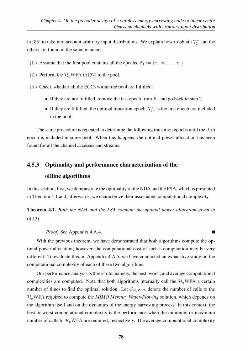
Chapter 4. On the precoder design of a wireless energy harvesting node in linear vectorGaussian channels with arbitrary input distribution
in [85] to take into account arbitrary input distributions. We explain how to obtain T ?2 and the
others are found in the same manner:
(1.) Assume that the first pool contains all the epochs, P1 := {τ1, τ2, . . . , τJ}.
(2.) Perform theHgWFA in [57] to the pool.
(3.) Check whether all the ECCs within the pool are fulfilled:
• If they are not fulfilled, remove the last epoch from P1 and go back to step 2.
• If they are fulfilled, the optimal transition epoch, T ?2 , is the first epoch not included
in the pool.
The same procedure is repeated to determine the following transition epochs until the J-th
epoch is included in some pool. When this happens, the optimal power allocation has been
found for all the channel accesses and streams.
4.5.3 Optimality and performance characterization of the
offline algorithms
In this section, first, we demonstrate the optimality of the NDA and the FSA, which is presented
in Theorem 4.1 and, afterwards, we characterize their associated computational complexity.
Theorem 4.1. Both the NDA and the FSA compute the optimal power allocation given in
(4.13).
Proof: See Appendix 4.A.4.
With the previous theorem, we have demonstrated that both algorithms compute the op-
timal power allocation; however, the computational cost of such a computation may be very
different. To evaluate this, in Appendix 4.A.5, we have conducted an exhaustive study on the
computational complexity of each of these two algorithms.
Our performance analysis is three-fold, namely, the best, worst, and average computational
complexities are computed. Note that both algorithms internally call the HgWFA a certain
number of times to find the optimal solution. Let CHgWFA denote the number of calls to the
HgWFA required to compute the MIMO Mercury Water-Flowing solution, which depends on
the algorithm itself and on the dynamics of the energy harvesting process. In this context, the
best or worst computational complexity is the performance when the minimum or maximum
number of calls to HgWFA are required, respectively. The average computational complexity
78
4.6. Online algorithm
Best Worst Average(Op.) (CHgWFA) (Op.) (CHgWFA) (CHgWFA )
NDA aNK J O( a2KNJ) 2J − 1E {CNDAHgWFA} = J(q + 1)− qvar{CNDAHgWFA} = (J − 1)q(1− q)
FSA aNK 1 O( a6KNJ2) J2+J
2
E {CFSAHgWFA} =(J2
2 + J2 − 1
)p+ 1
var{CFSAHgWFA} =(J2 + 1
)2(J − 1)p(1− p)
Table 4.1: Computational complexity of the NDA and the FSA in the best, worst and averagecase scenarios.
uses a probabilistic model to compute the average number of calls to HgWFA. Basically, for
the NDA we assume that there is a fixed probability q that the water level decreases from pool
to pool, whereas, for the FSA we assume that there is a fixed probability p that a certain ECC is
not satisfied. Both p and q can be experimentally adjusted depending on the energy harvesting
profile. The computational complexity in terms of operations (Op.), as well as, in terms of
CHgWFA is summarized in Table 4.1, where a is a constant parameter that depends, among
others, on the size of the MMSE table required to compute the inverse MMSE function and
on the tolerance used in the stopping criteria of the HgWFA. The details of the derivations
of the different computational complexities can be found in Appendix 4.A.5. In §4.7.2, the
theoretical results on the algorithms’ computational complexities are compared with the ones
obtained through simulation.
4.6 Online algorithm
Up to now, we have assumed that the transmitter has non-causal knowledge of both the CSI and
the EHI, which might be realistic in scenarios in which the energy source is predictable, cf.,
§2.1.3. Therefore, the MIMO Mercury Water-Flowing solution provides an upper bound on the
achievable mutual information of practical schemes in which VBn = IK . In this section, we
develop an online algorithm, which is strongly based on the optimal offline solution, the MIMO
Mercury Water-Flowing power allocation, but that does not require future knowledge of neither
the energy arrivals nor the channel state, that computes a suboptimal power allocation of the
problem in (4.11).
Let Fw be the flowing window that is an input parameter of the online algorithm that refers
to the number of channel accesses in which the water is allowed to flow, which can be obtained
by a previous training under the considered energy harvesting profile, and let an event denote
a channel access in which a change in the channel state is produced or an energy packet is
79
Chapter 4. On the precoder design of a wireless energy harvesting node in linear vectorGaussian channels with arbitrary input distribution
harvested, i.e.,
Et = {n|∆n−1 6= ∆n} ∪ {n|n = ej, j = 1, . . . , J}, t = 1, . . . , S,
where S ∈ [J,N ]. In this context, the proposed online algorithm proceeds as follows:
(1.) The initial energy in the battery, E1, is allocated to the different streams of the first Fwchannel accesses according to theHgWFA where the channel is expected to be static and
equal to the gain of the first channel use ∆n = ∆1,∀n ∈ [1, Fw].
(2.) When the transmitter detects an event, it updates the allocated power of the channel ac-
cesses n ∈ [Et,min{Et + Fw − 1, N}] by using the HgWFA with the remaining energy
in the battery and with the energy of the harvested packet (if the event is an energy ar-
rival), i.e.,∑
j|ej≤Et Ej − Ts∑Et−1
n=1
∑k pkn, and by assuming that the channel remains
constant during the flowing window, i.e., ∆n = ∆Et , ∀n ∈ [Et,min{Et + Fw − 1, N}].Note that the transmitter may stay silent in some channel accesses if the difference be-
tween two consecutive incoming energy packets is greater than the flowing window,
ej − ej−1 > Fw.11
(3.) Step (2.) is repeated until the N -th channel access is reached. The proposed online
algorithm satisfies the ECCs and, as pointed out, does not require future information of
neither the channel state nor the energy arrivals.
The performance in terms of achieved mutual information depends on the correctness of
the estimation of the flowing window, Fw, as discussed with the numerical analysis in §4.7. In
summary, this online algorithm provides us a lower bound on the mutual information that can
be achieved with sophisticated online algorithms that make use of precise statistical models of
the energy harvesting process and channel state. A myriad of works have dealt with channel
modeling; however, as it has been argued in §2.1.1, having a precise statistical model of the
energy harvesting process is indeed not trivial as it depends on many factors such as the har-
vester used by the node (e.g., a solar panel, piezoelectric generator, etc.), the node’s placement,
mobility, etc. According to this, to develop better online algorithms it is key that during the
following years statistical models of the energy harvesting process are developed, which must
capture the energy variability due to environmental and climatic conditions, and the node’s
placement and mobility.
11This situation rarely takes place in practice since, in most common situations, Fw is several times the meannumber of channel accesses per epoch. For example, in the simulated framework presented in §4.7, we haveobtained that Fw is 4.4 times the mean number of channel accesses per epoch.
80
4.7. Results
4.7 Results
This section first evaluates the gain of the proposed MIMO Mercury Water-Flowing solution
w.r.t. other suboptimal solutions and, secondly, it presents an analysis through simulation of
the computational complexity of the NDA and FSA.
4.7.1 Results on the MIMO Mercury Water-Flowing solution
In this section, we evaluate the mutual informations obtained with the optimal offline solution,
the MIMO Mercury Water-Flowing (Hg-WFlow), and with the online policy presented in §4.6.
To the best of our knowledge, there are no offline algorithms in the literature that max-
imize the mutual information by jointly considering energy harvesting at the transmitter and
arbitrary distributed input symbols. In this context, we use the following three algorithms,
which are optimal in different setups and have been adapted to the energy harvesting scenario,
as a reference to evaluate the mutual information achieved by the proposed offline and online
solutions:
• The DWF solution in (2.21) that is the optimal offline power allocation for a WEHN
when the distribution of the input symbols is Gaussian.
• Epoch-by-Epoch Water-Filling (EbE-WF) that uses the CWF power allocation in (2.10)
by forcing that the harvested energy in a certain epoch is expended in the channel ac-
cesses of that same epoch.
• Epoch-by-Epoch Mercury/Water-Filling (EbE-HgWF) where the power allocation is ob-
tained by using the HgWF solution in (2.13) and forcing that the harvested energy in a
certain epoch is expended in the channel accesses of that same epoch.
We have considered a channel matrix of rank K = 4, where the channel gains are uni-
formly distributed in (0, 1). The modulations used in each stream are BPSK, 4-PAM, 16-PAM,
and 32-PAM, respectively. The symbol duration is Ts = 10 ms and N = 100 channel accesses
have been considered during which a total of J = 40 energy packets are harvested. Energy
arrivals are uniformly distributed along the channel accesses and with random amounts of en-
ergy, which are normalized according to the total harvested energy that varies along the x-axis
of Figure 4.3. The y-axis shows the mutual information obtained with the different strategies.
After some training in this scenario, we have obtained that the optimal flowing window is
Fw = 11 channel accesses.
As shown in Figure 4.3, our proposed solution, theHg-WFlow, outperforms all the subop-
timal strategies. The improvement of theHg-WFlow w.r.t. the EbE-HgWF comes from letting
81

Chapter 4. On the precoder design of a wireless energy harvesting node in linear vectorGaussian channels with arbitrary input distribution
0 2 4 6 8 10 12 14 16 18 200
25
50
75
100
125
150
175
200
225
250
Total harvested energy (J)
Mutualinform
ation(n
at/sec)
Hg-WFlow
DWF
EbE-HgWF
EbE-WF
Online Fw = 11
Figure 4.3: Mutual information for the different transmission strategies versus total harvestedenergy.
the water to flow across epochs and, hence, it directly depends on the parameter J since the
higher is the number of epochs, the higher is the mutual information gain that can be achieved
by letting the water flow.12 The same happens with the improvement of the DWF w.r.t. EbE-
WF. On the other hand, the mutual information gain of the EbE-HgWF andHg-WFlow w.r.t.
their respective CWF strategies, EbE-WF and DWF, comes from the use of mercury in the
resource allocation. Thus, when the energy availability is low, both perform similarly because
the node is working in the low SNR regime in which the mutual information of finite alphabets
is well approximated by the mutual information of the Gaussian distribution [117]. However,
when the energy availability is high, the EbE-HgWF andHg-WFlow achieve a higher mutual
information than their respective CWF strategies since the mutual information of finite con-
stellations asymptotically saturates (not more than log2M bits of information can be sent per
channel use), cf., §2.2.1.2. Finally, note that, in spite of not having knowledge of the energy
arrivals nor channel state, the online power allocation performs close to the offline optimal
Hg-WFlow in the low SNR regime. When the available energy increases, the gap between the
MIMO Mercury Water-Flowing and the proposed online algorithm also increases, nevertheless
the online algorithm still presents a reasonably good mutual information outperforming any
Epoch-by-Epoch strategy.
12When J = 1, the solid and dashed curves overlap since there is only one epoch.
82
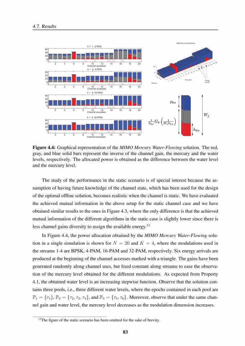
4.7. Results
2 4 6 8 10 12 14 16 18 20
0
20
40
60
k = 1, 2-PAM
Channel accesses
2 4 6 8 10 12 14 16 18 20
0
20
40
60
k = 2, 4-PAM
Channel accesses
2 4 6 8 10 12 14 16 18 20
0
20
40
60
k = 3, 16-PAM
Channel accesses
2 4 6 8 10 12 14 16 18 20
0
20
40
60
k = 4, 32-PAM
Channel accesses
12
34
56
78
910
1112
1314
1516
1718
1920
12
34
0
50
MIMO Mercury Waterflowing
Time Slots
Streams
Energyarrivals
Figure 4.4: Graphical representation of the MIMO Mercury Water-Flowing solution. The red,gray, and blue solid bars represent the inverse of the channel gain, the mercury and the waterlevels, respectively. The allocated power is obtained as the difference between the water leveland the mercury level.
The study of the performance in the static scenario is of special interest because the as-
sumption of having future knowledge of the channel state, which has been used for the design
of the optimal offline solution, becomes realistic when the channel is static. We have evaluated
the achieved mutual information in the above setup for the static channel case and we have
obtained similar results to the ones in Figure 4.3, where the only difference is that the achieved
mutual information of the different algorithms in the static case is slightly lower since there is
less channel gains diversity to assign the available energy.13
In Figure 4.4, the power allocation obtained by the MIMO Mercury Water-Flowing solu-
tion in a single simulation is shown for N = 20 and K = 4, where the modulations used in
the streams 1-4 are BPSK, 4-PAM, 16-PAM and 32-PAM, respectively. Six energy arrivals are
produced at the beginning of the channel accesses marked with a triangle. The gains have been
generated randomly along channel uses, but fixed constant along streams to ease the observa-
tion of the mercury level obtained for the different modulations. As expected from Property
4.1, the obtained water level is an increasing stepwise function. Observe that the solution con-
tains three pools, i.e., three different water levels, where the epochs contained in each pool are
P1 = {τ1}, P2 = {τ2, τ3, τ4}, and P3 = {τ5, τ6}. Moreover, observe that under the same chan-
nel gain and water level, the mercury level decreases as the modulation dimension increases.
13The figure of the static scenario has been omitted for the sake of brevity.
83
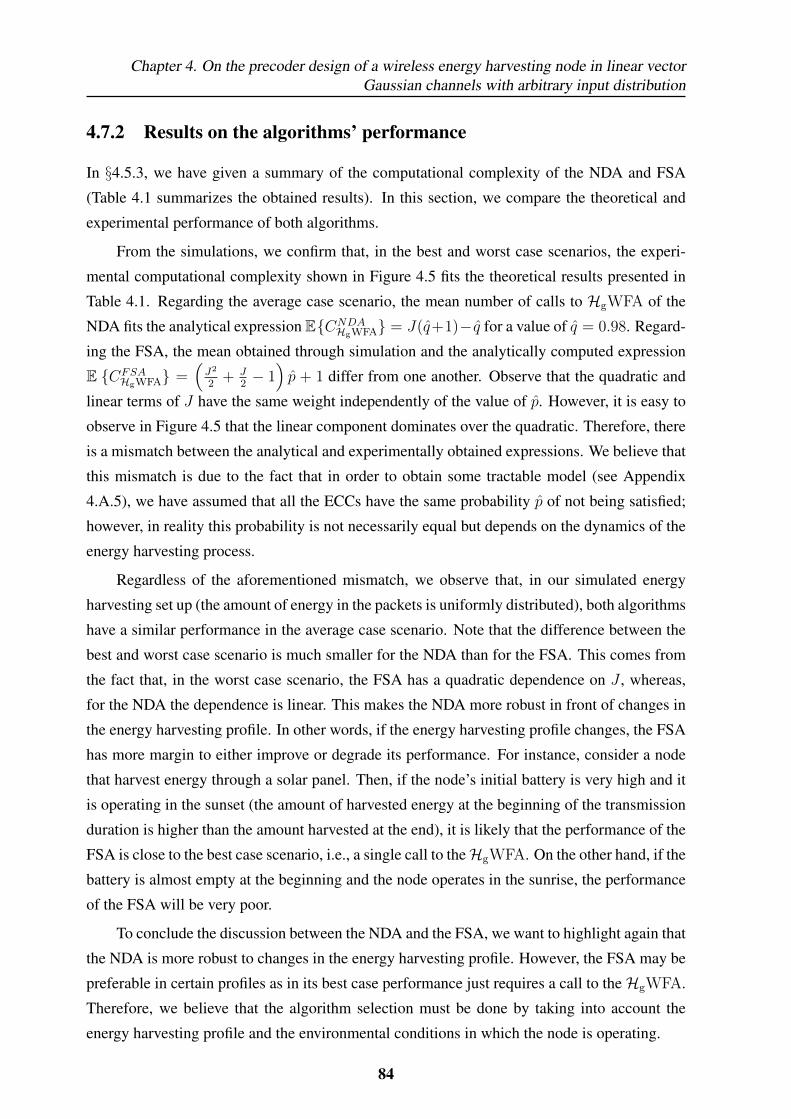
Chapter 4. On the precoder design of a wireless energy harvesting node in linear vectorGaussian channels with arbitrary input distribution
4.7.2 Results on the algorithms’ performance
In §4.5.3, we have given a summary of the computational complexity of the NDA and FSA
(Table 4.1 summarizes the obtained results). In this section, we compare the theoretical and
experimental performance of both algorithms.
From the simulations, we confirm that, in the best and worst case scenarios, the experi-
mental computational complexity shown in Figure 4.5 fits the theoretical results presented in
Table 4.1. Regarding the average case scenario, the mean number of calls to HgWFA of the
NDA fits the analytical expression E{CNDAHgWFA} = J(q+1)− q for a value of q = 0.98. Regard-
ing the FSA, the mean obtained through simulation and the analytically computed expression
E {CFSAHgWFA} =
(J2
2+ J
2− 1)p + 1 differ from one another. Observe that the quadratic and
linear terms of J have the same weight independently of the value of p. However, it is easy to
observe in Figure 4.5 that the linear component dominates over the quadratic. Therefore, there
is a mismatch between the analytical and experimentally obtained expressions. We believe that
this mismatch is due to the fact that in order to obtain some tractable model (see Appendix
4.A.5), we have assumed that all the ECCs have the same probability p of not being satisfied;
however, in reality this probability is not necessarily equal but depends on the dynamics of the
energy harvesting process.
Regardless of the aforementioned mismatch, we observe that, in our simulated energy
harvesting set up (the amount of energy in the packets is uniformly distributed), both algorithms
have a similar performance in the average case scenario. Note that the difference between the
best and worst case scenario is much smaller for the NDA than for the FSA. This comes from
the fact that, in the worst case scenario, the FSA has a quadratic dependence on J , whereas,
for the NDA the dependence is linear. This makes the NDA more robust in front of changes in
the energy harvesting profile. In other words, if the energy harvesting profile changes, the FSA
has more margin to either improve or degrade its performance. For instance, consider a node
that harvest energy through a solar panel. Then, if the node’s initial battery is very high and it
is operating in the sunset (the amount of harvested energy at the beginning of the transmission
duration is higher than the amount harvested at the end), it is likely that the performance of the
FSA is close to the best case scenario, i.e., a single call to theHgWFA. On the other hand, if the
battery is almost empty at the beginning and the node operates in the sunrise, the performance
of the FSA will be very poor.
To conclude the discussion between the NDA and the FSA, we want to highlight again that
the NDA is more robust to changes in the energy harvesting profile. However, the FSA may be
preferable in certain profiles as in its best case performance just requires a call to theHgWFA.
Therefore, we believe that the algorithm selection must be done by taking into account the
energy harvesting profile and the environmental conditions in which the node is operating.
84
4.8. Conclusions
0 50 100 150 200 250 3000
100
200
300
400
500
600
700
800
J (N = 300)
CH
gW
FA
Performance of the algorithms
NDA - Worst
NDA - Average
NDA - Best
FSA - Worst
FSA - Average
FSA - Best
Figure 4.5: Analysis of the performance of the NDA and FSA in terms of CHgWFA.
4.8 Conclusions
In this chapter, we have considered a WEHN transmitting arbitrarily distributed symbols in
a discrete-time linear vector Gaussian channel. We have studied the precoding strategy that
maximizes the mutual information by taking into account causality constraints on the use of
energy. We have proved that the optimal left singular vectors of the precoder matrix diagonal-
ize the channel, similarly as in the optimal precoder for the case of non-harvesting nodes. We
have derived the expression[∆2
nVTBn
EnVBn
]kk
= 1Wj
that relates the singular values of the
precoder (through the MMSE matrix) with the energy harvesting profile (through the different
water levels). The derivation of the optimal right singular vectors, V?Bn
, is left as an open prob-
lem. Then, we have derived the MIMO Mercury Water-Flowing solution, the optimal power
allocation when VBn = IK , which can be expressed in closed form and accepts an intuitive
graphical interpretation based on the fact that the power allocation in a certain stream is the
difference between the water level and the mercury level, which, as shown in this chapter, is
a monotonically increasing function of the water level. Additionally, we have developed two
different algorithms that compute the MIMO Mercury Water-Flowing solution and we have an-
alytically and experimentally evaluated their computational complexity. We have also proposed
an online algorithm that only requires causal knowledge of the energy harvesting process and
channel state. Finally, through numerical simulations, we have shown a substantial increase in
85
Chapter 4. On the precoder design of a wireless energy harvesting node in linear vectorGaussian channels with arbitrary input distribution
the mutual information w.r.t. other suboptimal offline strategies, which do not account for the
shape, size and distribution of the input symbol or do not exploit the water level equalization
across epochs, and we have seen that the mutual information achieved with the online algorithm
is close to the one of the MIMO Mercury Water-Flowing solution.
4.A Appendix
4.A.1 Proof of Lemma 4.1
Let us assume that the optimal precoding matrices of the channel accesses n = 2, . . . , N are
known, i.e., {B?n}Nn=2. Then, we focus on finding the optimal precoding matrix of the first
channel use B?1. The problem in (4.4) is equivalent to
maximizeB1
I(s1; y1) + a (4.15a)
subject to TsTr(B1BT1 ) + b+ c(`) ≤
∑j=1
Ej, ` = 1, . . . , J,
where a, b and c(`) do not depend on B1. By only keeping the most restrictive constraint,
which is denoted by P , the previous optimization problem reduces to
maximizeB1
I(s1; y1) (4.16a)
subject to Tr(B1BT1 ) ≤ P . (4.16b)
Finally, once the problem is expressed as (4.16), it is known from [58, Prp. 1] that the left
singular vectors of B?1 can be chosen to coincide with the eigenvectors of the channel Gram
matrix, i.e., UB1 = UG1 . A similar approach can be applied to show that {B?n}Nn=2 diagonalize
their respective channels.
4.A.2 Proof of Lemma 4.2
By applying the chain rule, we have that
DpnI(sn; Gnsn + wn) = DGnI(sn; Gnsn + wn) DpnGn.
86
4.A. Appendix
The first term in the previous equation can be easily derived from (2.12) as
DGnI(sn; Gnsn + wn) = vecT(GnEn).
The second term, DpnGn, is
DpnGn =1
2(VBn ⊗VGn∆n)SKDiag(σ−1
n ) (4.17)
=1
2(VBn ⊗VGn∆n)SKDiag(diag(Σ−1
n )) (4.18)
=1
2(VBn ⊗VGn∆n)SKSTK(IK ⊗Σ−1
n )SK (4.19)
=1
2(VBn ⊗VGn∆n)(IK ⊗Σ−1
n )SK , (4.20)
where (4.17) can be proved in a similar manner to DλP in [76, Proof of Theorem 5] with
SK ∈ RK2×K being the reduction matrix introduced in [76] (see Appendix 4.A.6 for a concise
summary on the properties of SK). In (4.19) and (4.20), we have applied Properties 6 and 8 in
Appendix 4.A.6, respectively.
Therefore, we have that DpnI(sn; Gnsn + wn) is
DpnI(sn; Gnsn + wn) =1
2vecT(GnEn) (VBn ⊗VGn∆n)
(IK ⊗Σ−1
n
)SK (4.21)
=1
2vecT(GnEn)
(VBn ⊗VGn∆nΣ
−1n
)SK (4.22)
=1
2vecT
((VGn∆nΣ
−1n )TGnEnVBn
)SK (4.23)
=1
2vecT
(∆2
nVTBn
EnVBn
)SK =
1
2diagT
(∆2
nVTBn
EnVBn
),(4.24)
where, in (4.22) and (4.23), we have used that (A⊗B)(C⊗D) = AC⊗BD and vec(ABC) =
(CT ⊗A)vecB for any matrices A, B, C, and D such that the matrix products AC, BD, and
ABC are well defined [116]. Finally, (4.24) follows from the definition of the reduction matrix
(see Appendix 4.A.6). This concludes the proof.
4.A.3 Proof of Lemma 4.3
Let ψ be some fixed MMSE that can be obtained as
ψ = mmseG(snrG) = mmseA(snrA), (4.25)
87

Chapter 4. On the precoder design of a wireless energy harvesting node in linear vectorGaussian channels with arbitrary input distribution
wheremmseG(snrG) andmmseA(snrA) give the MMSE as a function of the SNR for a Gaus-
sian and for an arbitrary input distribution, respectively. Thus, snrG and snrA are the associated
required SNRs to achieve the error ψ for these distributions.
Similarly, the required SNR to obtain a certain error can be computed by the inverse
MMSE function as snrG = mmse−1G (ψ) and snrA = mmse−1
A (ψ).
For the Gaussian case, it is broadly known that ψ = mmseG(snrG) = 11+snrG
with deriva-
tive dmmseG(snrG)dsnrG
= −1(1+snrG)2
. Similarly, snrG = mmse−1G (ψ) = 1
ψ− 1 and dmmse−1
G (ψ)
dψ = −1ψ2 .
Note that for any generic function f(x), such that f(x) and f−1(x) are differentiable, it is
verified that df−1(f(x))dx = df−1(f(x))
df(x)df(x)
dx = 1. By applying the previous property, the following
relation is obtained:
dmmse−1G (ψ)
dψdmmseG(snrG)
dsnrG=
dmmse−1A (ψ)
dψdmmseA(snrA)
dsnrA.
Recall that G(ψ) = 1ψ−mmse−1
A (ψ) as ψ ∈ [0, 1]. Then, its derivative is
dG(ψ)
dψ=−1
ψ2− dmmse−1
A (ψ)
dψ=
dmmse−1G (ψ)
dψ− dmmse−1
A (ψ)
dψ
=
dmmse−1G (ψ)
dψdmmseA(snrA)
dsnrA
(dmmseA(snrA)
dsnrA− dmmseG(snrG)
dsnrG
).
In [118], it was recently shown that mmseA(snrA) = E{M2} and dmmseA(snrA)dsnrA
= −E{M22},
where M2 = var{x|√snrAx+ n}. Therefore, the first term of the previous equation is always
nonnegative since both the MMSE and the inverse MMSE functions are decreasing for any
distribution. Accordingly, we have that
sign
(dG(ψ)
dψ
)= sign
(dmmseA(snrA)
dsnrA− dmmseG(snrG)
dsnrG
)(4.26)
= sign
(dmmseA(snrA)
dsnrA+
1
(1 + snrG)2
)(4.27)
= sign
(dmmseA(snrA)
dsnrA+mmseA(snrA)2
)(4.28)
= sign(−E{M2
2}+ (E{M2})2) = sign (−var{M2}) , (4.29)
where in (4.28), we have used that snrG = 1mmseA(snrA)
− 1, which follows from (4.25). In
(4.29), we have used the recently found expressions of the MMSE and its derivative [118].
Finally, as the variance is nonnegative, dG(ψ)dψ ≤ 0 and G(ψ) is a monotonically decreasing
function.
88
4.A. Appendix
4.A.4 Proof of Theorem 4.1
The optimality of the algorithms is proved by demonstrating that the power allocation obtained
by means of each of the algorithms satisfies the KKT sufficient optimality conditions:
(1.) ∂L∂pkn
= 0, ∀k, n.
(2.) Ts∑`
j=1
∑n∈τj
∑Kk=1 pkn ≤
∑`j=1 Ej , ` = 1, . . . , J .
(3.) λ` ≥ 0, ` = 1, . . . , J .
(4.) λ`(Ts∑`
j=1
∑n∈τj
∑Kk=1 pkn −
∑`j=1 Ej
)= 0, ` = 1, . . . , J .
Moreover, we know that by the end of the transmission the battery must be empty since,
otherwise, the remaining energy in the battery can be used to increase the total mutual infor-
mation. Thus, (2.) must be met with equality for ` = J . Note that both algorithms compute a
power allocation strategy that satisfies the ECCs and that by the end of the last channel access
all the energy has been used. Therefore, (2.) is satisfied ∀` and it is satisfied with equality for
` = J . From Property 4.1, if the water level is non-decreasing in time, then (3.) can be verified.
In the NDA, the water level is clearly non-decreasing in time. Regarding the FSA, if some ECC
is not satisfied, it is because the water level must be reduced before the point where the ECC is
not satisfied and increased afterwards. Indeed, this is what the algorithm does in the procedure
of finding the optimal pools. Therefore, (3.) is also satisfied in the FSA. Finally, since both
algorithms compute the optimal power allocation within a pool by using the HgWFA, where
the water level is found by forcing that all the available energy must be used by the end of the
pool, conditions (1.) and (4.) are satisfied. With this, we have demonstrated that the power
allocation computed by the NDA and the FSA is the optimal power allocation.
4.A.5 Computational complexity of the algorithms
In this appendix, we study the performance of the two algorithms that compute the MIMO
Mercury Water-Flowing solution, the NDA and the FSA.
We have carried out a three-fold analysis, namely, the best, worst and average computa-
tional complexity. As mentioned before, both algorithms internally call the HgWFA a certain
number of times to find the optimal solution. The performance is evaluated in terms of op-
erations and number of calls to the HgWFA required to compute the MIMO Mercury Water-
Flowing solution, CHgWFA.
89
Chapter 4. On the precoder design of a wireless energy harvesting node in linear vectorGaussian channels with arbitrary input distribution
Before getting into the complexity of each of the aforementioned scenarios, let us first
compute the complexity of the HgWFA when the algorithm computes the power allocation of
NK parallel channels, i.e.,
CCHgWF(N,K) = aNK, (4.30)
where a is a constant parameter that depends, among others, on the size of the MMSE table
required to compute the inverse MMSE function mmse−1k (·) and on the tolerance used in the
stopping criteria of theHgWFA. Now, let us proceed to compute the computational complexity
of the NDA and FSA.
4.A.5.1 Computational complexity in the best case scenario
NDA: The best case scenario for the NDA occurs when the resulting water levels of applying
the HgWFA at each epoch are non-decreasing throughout all the transmission. Thus, the best
case computational complexity for the NDA is
CCBNDA(N,K, J) =
J∑j=1
CCHgWF(Lj, K) =J∑j=1
aLjK = aNK, (4.31)
where Lj is the number of channel accesses contained in τj and, accordingly,∑J
j=1 Lj = N .
Note that the number of calls to theHgWFA is CHgWFA = J.
FSA: Regarding the FSA the best performance is obtained when the algorithm can stop at
the first iteration, i.e., after applying the HgWFA to the N channel accesses it is observed that
the resulting power allocation satisfies all the ECCs. Thus, we have that
CCBFSA(N,K, J) = CCHgWF(N,K) = aNK. (4.32)
Note that the number of calls to theHgWFA for the FSA in the best case scenario is CHgWFA =
1.
Observe that, even though CHgWFA differs from one algorithm to another, they achieve
the same computational complexity in terms of operations in the best case scenario. However,
note that the best case scenario for the FSA occurs when the water level of the optimal power
allocation remains constant throughout all the transmission time, in other words, there is a
single pool. However, the best case scenario for the NDA is completely the opposite, the water
level is different at every epoch and, thus, the total number of pools is J .
90
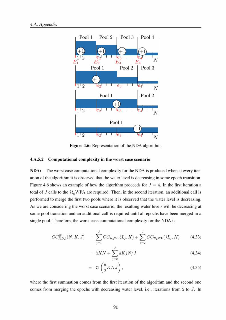
4.A. Appendix
Figure 4.6: Representation of the NDA algorithm.
4.A.5.2 Computational complexity in the worst case scenario
NDA: The worst case computational complexity for the NDA is produced when at every iter-
ation of the algorithm it is observed that the water level is decreasing in some epoch transition.
Figure 4.6 shows an example of how the algorithm proceeds for J = 4. In the first iteration a
total of J calls to the HgWFA are required. Then, in the second iteration, an additional call is
performed to merge the first two pools where it is observed that the water level is decreasing.
As we are considering the worst case scenario, the resulting water levels will be decreasing at
some pool transition and an additional call is required until all epochs have been merged in a
single pool. Therefore, the worst case computational complexity for the NDA is
CCWNDA(N,K, J) =
J∑j=1
CCHgWF(Lj, K) +J∑j=2
CCHgWF(jLj, K) (4.33)
= aKN +J∑j=2
aKjN/J (4.34)
= O(a
2KNJ
), (4.35)
where the first summation comes from the first iteration of the algorithm and the second one
comes from merging the epochs with decreasing water level, i.e., iterations from 2 to J . In
91
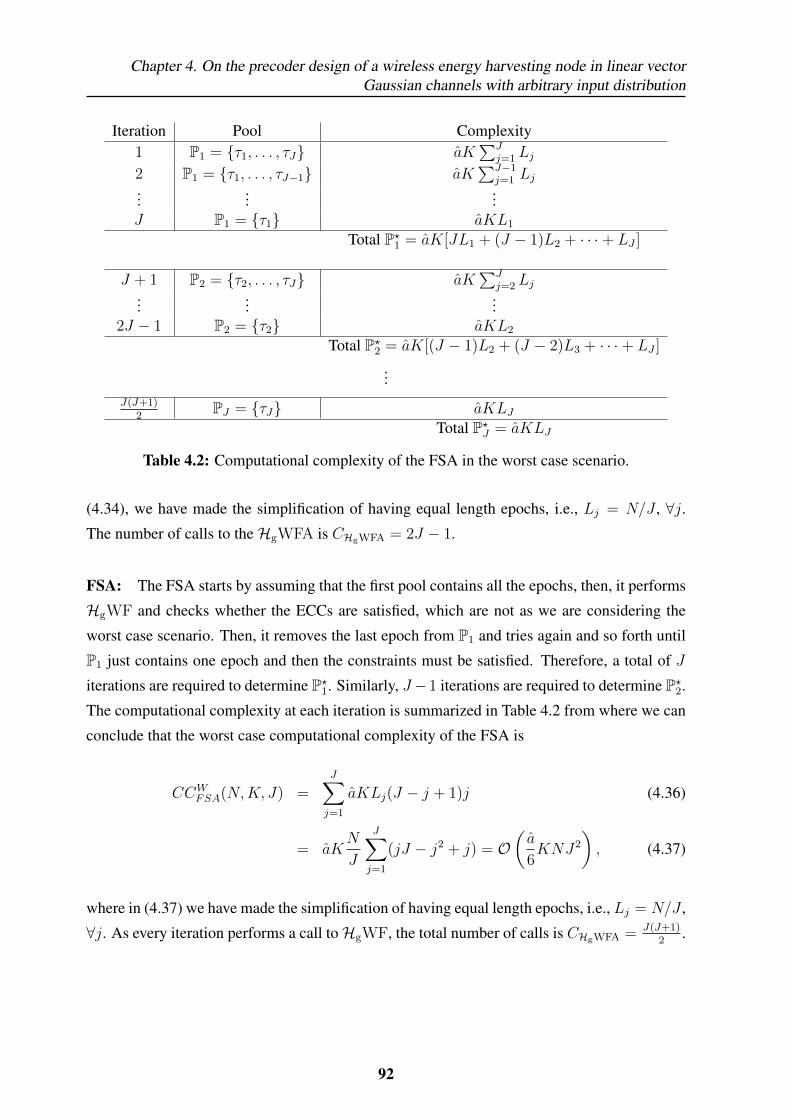
Chapter 4. On the precoder design of a wireless energy harvesting node in linear vectorGaussian channels with arbitrary input distribution
Iteration Pool Complexity1 P1 = {τ1, . . . , τJ} aK
∑Jj=1 Lj
2 P1 = {τ1, . . . , τJ−1} aK∑J−1
j=1 Lj...
......
J P1 = {τ1} aKL1
Total P?1 = aK[JL1 + (J − 1)L2 + · · ·+ LJ ]
J + 1 P2 = {τ2, . . . , τJ} aK∑J
j=2 Lj...
......
2J − 1 P2 = {τ2} aKL2
Total P?2 = aK[(J − 1)L2 + (J − 2)L3 + · · ·+ LJ ]
...J(J+1)
2PJ = {τJ} aKLJ
Total P?J = aKLJ
Table 4.2: Computational complexity of the FSA in the worst case scenario.
(4.34), we have made the simplification of having equal length epochs, i.e., Lj = N/J , ∀j.The number of calls to theHgWFA is CHgWFA = 2J − 1.
FSA: The FSA starts by assuming that the first pool contains all the epochs, then, it performs
HgWF and checks whether the ECCs are satisfied, which are not as we are considering the
worst case scenario. Then, it removes the last epoch from P1 and tries again and so forth until
P1 just contains one epoch and then the constraints must be satisfied. Therefore, a total of J
iterations are required to determine P?1. Similarly, J−1 iterations are required to determine P?2.
The computational complexity at each iteration is summarized in Table 4.2 from where we can
conclude that the worst case computational complexity of the FSA is
CCWFSA(N,K, J) =
J∑j=1
aKLj(J − j + 1)j (4.36)
= aKN
J
J∑j=1
(jJ − j2 + j) = O(a
6KNJ2
), (4.37)
where in (4.37) we have made the simplification of having equal length epochs, i.e., Lj = N/J ,
∀j. As every iteration performs a call toHgWF, the total number of calls is CHgWFA = J(J+1)2
.
92
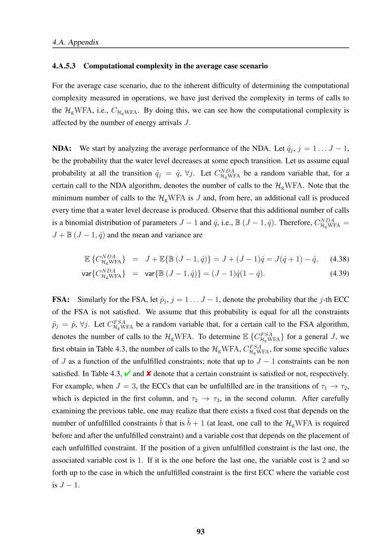
4.A. Appendix
4.A.5.3 Computational complexity in the average case scenario
For the average case scenario, due to the inherent difficulty of determining the computational
complexity measured in operations, we have just derived the complexity in terms of calls to
the HgWFA, i.e., CHgWFA. By doing this, we can see how the computational complexity is
affected by the number of energy arrivals J .
NDA: We start by analyzing the average performance of the NDA. Let qj , j = 1 . . . J − 1,
be the probability that the water level decreases at some epoch transition. Let us assume equal
probability at all the transition qj = q, ∀j. Let CNDAHgWFA be a random variable that, for a
certain call to the NDA algorithm, denotes the number of calls to the HgWFA. Note that the
minimum number of calls to the HgWFA is J and, from here, an additional call is produced
every time that a water level decrease is produced. Observe that this additional number of calls
is a binomial distribution of parameters J − 1 and q, i.e., B (J − 1, q). Therefore, CNDAHgWFA =
J + B (J − 1, q) and the mean and variance are
E {CNDAHgWFA} = J + E{B (J − 1, q)} = J + (J − 1)q = J(q + 1)− q, (4.38)
var{CNDAHgWFA} = var{B (J − 1, q)} = (J − 1)q(1− q). (4.39)
FSA: Similarly for the FSA, let pj , j = 1 . . . J − 1, denote the probability that the j-th ECC
of the FSA is not satisfied. We assume that this probability is equal for all the constraints
pj = p, ∀j. Let CFSAHgWFA be a random variable that, for a certain call to the FSA algorithm,
denotes the number of calls to the HgWFA. To determine E {CFSAHgWFA} for a general J , we
first obtain in Table 4.3, the number of calls to theHgWFA, CFSAHgWFA, for some specific values
of J as a function of the unfulfilled constraints; note that up to J − 1 constraints can be non
satisfied. In Table 4.3, 4 and 8 denote that a certain constraint is satisfied or not, respectively.
For example, when J = 3, the ECCs that can be unfulfilled are in the transitions of τ1 → τ2,
which is depicted in the first column, and τ2 → τ3, in the second column. After carefully
examining the previous table, one may realize that there exists a fixed cost that depends on the
number of unfulfilled constraints b that is b + 1 (at least, one call to the HgWFA is required
before and after the unfulfilled constraint) and a variable cost that depends on the placement of
each unfulfilled constraint. If the position of a given unfulfilled constraint is the last one, the
associated variable cost is 1. If it is the one before the last one, the variable cost is 2 and so
forth up to the case in which the unfulfilled constraint is the first ECC where the variable cost
is J − 1.
93
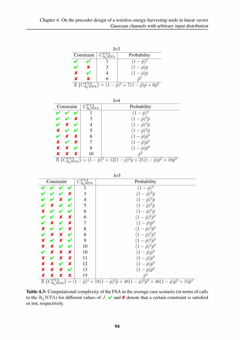
Chapter 4. On the precoder design of a wireless energy harvesting node in linear vectorGaussian channels with arbitrary input distribution
J=3Constraint CFSA
HgWFA Probability4 4 1 (1− p)2
4 8 3 (1− p)p8 4 4 (1− p)p8 8 6 p2
E {CFSAHgWFA} = (1− p)2 + 7(1− p)p+ 6p2
J=4Constraint CFSA
HgWFA Probability4 4 4 1 (1− p)3
4 4 8 3 (1− p)2p4 8 4 4 (1− p)2p8 4 4 5 (1− p)2p4 8 8 6 (1− p)p2
8 4 8 7 (1− p)p2
8 8 4 8 (1− p)p2
8 8 8 10 p3
E {CFSAHgWFA} = (1− p)3 + 12(1− p)2p+ 21(1− p)p2 + 10p3
J=5Constraint CFSA
HgWFA Probability4 4 4 4 1 (1− p)4
4 4 4 8 3 (1− p)3p4 4 8 4 4 (1− p)3p4 8 4 4 5 (1− p)3p8 4 4 4 6 (1− p)3p4 4 8 8 6 (1− p)2p2
4 8 4 8 7 (1− p)p2
8 4 4 8 8 (1− p)2p2
4 8 8 4 8 (1− p)2p2
8 4 8 4 9 (1− p)2p2
8 8 4 4 10 (1− p)2p2
4 8 8 8 10 (1− p)p3
8 4 8 8 11 (1− p)p3
8 8 4 8 12 (1− p)p3
8 8 8 4 13 (1− p)p3
8 8 8 8 15 p4
E {CFSAHgWFA} = (1− p)4 + 18(1− p)3p+ 48(1− p)2p2 + 46(1− p)p3 + 15p4
Table 4.3: Computational complexity of the FSA in the average case scenario (in terms of callsto the HgWFA) for different values of J . 4 and 8 denote that a certain constraint is satisfiedor not, respectively.
94
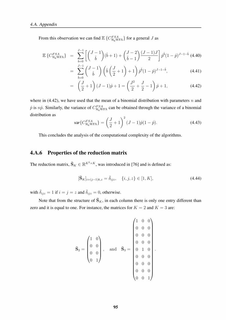
4.A. Appendix
From this observation we can find E {CFSAHgWFA} for a general J as
E {CFSAHgWFA} =
J−1∑b=0
[(J − 1
b
)(b+ 1) +
(J − 2
b− 1
)(J − 1)J
2
]pb(1− p)J−1−b (4.40)
=J−1∑b=0
(J − 1
b
)(b
(J
2+ 1
)+ 1
)pb(1− p)J−1−b, (4.41)
=
(J
2+ 1
)(J − 1)p+ 1 =
(J2
2+J
2− 1
)p+ 1, (4.42)
where in (4.42), we have used that the mean of a binomial distribution with parameters n and
p is np. Similarly, the variance of CFSAHgWFA can be obtained through the variance of a binomial
distribution as
var{CFSAHgWFA} =
(J
2+ 1
)2
(J − 1)p(1− p). (4.43)
This concludes the analysis of the computational complexity of the algorithms.
4.A.6 Properties of the reduction matrix
The reduction matrix, SK ∈ RK2×K , was introduced in [76] and is defined as:
[SK ]i+(j−1)k,z = δijz, {i, j, z} ∈ [1, K], (4.44)
with δijz = 1 if i = j = z and δijz = 0, otherwise.
Note that from the structure of SK , in each column there is only one entry different than
zero and it is equal to one. For instance, the matrices for K = 2 and K = 3 are:
S2 =
1 0
0 0
0 0
0 1
, and S3 =
1 0 0
0 0 0
0 0 0
0 0 0
0 1 0
0 0 0
0 0 0
0 0 0
0 0 1
.
95
Chapter 4. On the precoder design of a wireless energy harvesting node in linear vectorGaussian channels with arbitrary input distribution
The reduction matrix is designed so that
STKvec(A) = diag(A) (4.45)
for A ∈ RK×K . In this appendix, we summarize some additional properties of the reduction
matrix:
Property 4.3. Multiplication properties:
• Let A ∈ RK2×R, then the multiplication STKA removes K2 −K rows of A.
• Let A ∈ RK×R, then the multiplication SKA adds K2 −K rows of zeros to A.
• Let A ∈ RR×K , then the multiplication ASTK adds K2 −K columns of zeros to A.
• Let A ∈ RR×K2 , then the multiplication ASK removes K2 −K columns of A.
Proof: The proof follows directly from the structure of the reduction matrix.
Property 4.4. Let A ∈ RK×R, B ∈ RK×R, then STK (A⊗B) SK = A ◦B.
Proof: See [76, Lemma A.2].
Property 4.5. STKSK = IK .
Proof: The proof directly follows from setting A = IK and B = IK in Property 4.4.
Property 4.6. Let A ∈ RK×K , then STK(A⊗ IK)SK = Diag(diag(A)).
Proof: The proof directly follows from setting B = IK in Property 4.4.
Property 4.7. Let v ∈ RK , then STK(v ⊗ IK) = Diag(v).
Proof: The Kronecker product expands the vector v in a K2 ×K matrix that stacks
K diagonal matrices. Then, the multiplication by STK eliminates rows (see Property 4.3) so that
the resulting matrix is Diag(v).
Property 4.8. Let A ∈ RK2×K2 be a diagonal matrix, then SKSTKASK = ASK
Proof: From Property 4.3, STKA removes rows from A. Then, the product by the left
by SK adds rows of zeros. As a result, SKSTKA ∈ RK2×K2 zeroes K2−K rows of A. Finally,
the product with SK from the right removes K2 − K columns. As A is diagonal, the entries
that are modified by multiplying from the left by SKSTK are later removed by multiplying from
the right by SK . Therefore, SKSTKASK is equal to ASK , which directly removes the columns.
96
Chapter 5On the optimal resource allocation for a
wireless energy harvesting node considering
the circuitry power consumption
5.1 Introduction
Most transmission strategies like the MIMO Mercury Water-Flowing presented in the previous
chapter or the well-known CWF,HgWF, and DWF (cf. §2.2.1 and §2.3 [57, 84]) consider that
the radiated power is the unique source of energy consumption at the transmitter. Nevertheless,
as it has been argued in §2.1.4, this is a reasonable assumption only when the link distance is
large; in short-range communications, the remaining energy sinks at the transmitter, such as the
energetic cost associated with having the transceiver “on” in a certain channel access, must be
also accounted for in the design, as it was done in the Glue pouring strategy for non-harvesting
nodes (cf. §2.2.1.3 [50, 51]).
According to this, the aim of this chapter is to study and analyze the impact of other
sources of energy consumption at the transmitter (apart from the radiated power) over the
transmission strategy that maximizes the mutual information in a point-to-point link through a
discrete-time fading channel composed of several parallel independent streams.
In particular, since we consider several parallel subchannels at each channel access, we
generalize the power consumption model C1 presented in (2.4), to account not only for the
channel access activation cost but also for the activation cost of each parallel subchannel.
As it has been argued in the state of the art in Chapter 2, recently, a few works have studied
the impact of the channel access activation cost in point-to-point links with energy harvesting at
97
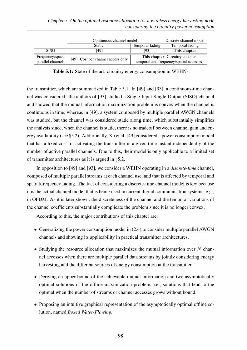
Chapter 5. On the optimal resource allocation for a wireless energy harvesting nodeconsidering the circuitry power consumption
Continuous channel model Discrete channel modelStatic Temporal fading Temporal fading
SISO [49] [93] This chapterFrequency/space [49]: Cost per channel access only This chapter: Circuitry cost perparallel channels temporal and frequency/spatial accesses
Table 5.1: State of the art: circuitry energy consumption in WEHNs
the transmitter, which are summarized in Table 5.1. In [49] and [93], a continuous-time chan-
nel was considered: the authors of [93] studied a Single-Input Single-Output (SISO) channel
and showed that the mutual information maximization problem is convex when the channel is
continuous in time; whereas in [49], a system composed by multiple parallel AWGN channels
was studied, but the channel was considered static along time, which substantially simplifies
the analysis since, when the channel is static, there is no tradeoff between channel gain and en-
ergy availability (see §5.2). Additionally, Xu et al. [49] considered a power consumption model
that has a fixed cost for activating the transmitter in a given time instant independently of the
number of active parallel channels. Due to this, their model is only applicable to a limited set
of transmitter architectures as it is argued in §5.2.
In opposition to [49] and [93], we consider a WEHN operating in a discrete-time channel,
composed of multiple parallel streams at each channel use, and that is affected by temporal and
spatial/frequency fading. The fact of considering a discrete-time channel model is key because
it is the actual channel model that is being used in current digital communication systems, e.g.,
in OFDM. As it is later shown, the discreteness of the channel and the temporal variations of
the channel coefficients substantially complicate the problem since it is no longer convex.
According to this, the major contributions of this chapter are:
• Generalizing the power consumption model in (2.4) to consider multiple parallel AWGN
channels and showing its applicability in practical transmitter architectures.
• Studying the resource allocation that maximizes the mutual information over N chan-
nel accesses when there are multiple parallel data streams by jointly considering energy
harvesting and the different sources of energy consumption at the transmitter.
• Deriving an upper bound of the achievable mutual information and two asymptotically
optimal solutions of the offline maximization problem, i.e., solutions that tend to the
optimal when the number of streams or channel accesses grows without bound.
• Proposing an intuitive graphical representation of the asymptotically optimal offline so-
lution, named Boxed Water-Flowing.
98
5.2. System model and problem formulation
• Implementing an online algorithm that achieves a mutual information that is close to the
one achieved by the optimal offline solution.
• Evaluating and comparing the computational complexities of the proposed strategies.
This chapter is structured as follows. In §5.2, the system model and problem formulation
are presented. The offline resource allocation problem is studied in §5.3 from two perspectives:
integer relaxation (§5.3.1) and through the dual problem (§5.3.2). A graphical interpretation of
the offline solution is presented in §5.3.3. In §5.4, the online solution is presented. The mutual
information and computational requirements of the different algorithms are evaluated in §5.5.
Finally, the chapter is concluded in §5.6.
5.2 System model and problem formulation
We consider a WEHN transmitting in a point-to-point link in which, at each channel access, the
communication channel can be decomposed into a set of K parallel non-interfering streams by
performing some joint signal processing at the transmitter and receiver, e.g., by using OFDM
or by diagonalizing a MIMO channel.
Let ykn be the channel output of the k-th stream at the n-th channel access, i.e.,
ykn =√pkngknxkn + wkn, k = 1, . . . , K, n = 1, . . . , N,
where xkn is the input symbol with E{||xkn||2} = 1; pkn is the radiated power; gkn is the
complex channel response with hkn = ||gkn||2 being the channel power gain; and wkn ∼CN (0, 1) is the noise. First, in §5.3, we assume that the transmitter has non-causal knowledge
of all the channel gains. This assumption is removed in §5.4 for the design of the online
algorithm.
As in the previous chapters, we characterize the energy harvesting process at the trans-
mitter with the packetized model introduced in §2.1.1, which is depicted in Figure 2.13, and
assume an ideal energy storage that has an infinite capacity and no imperfections.
The power consumption at the transmitter depends on its hardware and software archi-
tecture. As we focus on architectures with multiple data streams, it naturally follows that the
transmitter may experience either a power consumption associated with the channel access ac-
tivation, α, or a power consumption associated with the activation of each of the streams, β, or
both simultaneously.
In this context, we propose a power consumption model that, as shown later, can be applied
to several transmitter architectures, which is a generalization of C1 in (2.5) to scenarios in which
99
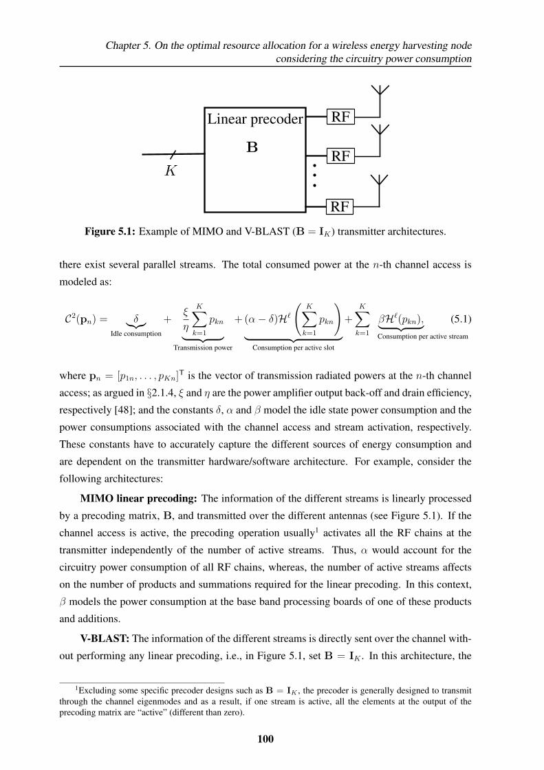
Chapter 5. On the optimal resource allocation for a wireless energy harvesting nodeconsidering the circuitry power consumption
Figure 5.1: Example of MIMO and V-BLAST (B = IK) transmitter architectures.
there exist several parallel streams. The total consumed power at the n-th channel access is
modeled as:
C2(pn) = δ︸︷︷︸Idle consumption
+ξ
η
K∑k=1
pkn︸ ︷︷ ︸Transmission power
+ (α− δ)H`
(K∑k=1
pkn
)︸ ︷︷ ︸
Consumption per active slot
+K∑k=1
βH`(pkn),︸ ︷︷ ︸Consumption per active stream
(5.1)
where pn = [p1n, . . . , pKn]T is the vector of transmission radiated powers at the n-th channel
access; as argued in §2.1.4, ξ and η are the power amplifier output back-off and drain efficiency,
respectively [48]; and the constants δ, α and β model the idle state power consumption and the
power consumptions associated with the channel access and stream activation, respectively.
These constants have to accurately capture the different sources of energy consumption and
are dependent on the transmitter hardware/software architecture. For example, consider the
following architectures:
MIMO linear precoding: The information of the different streams is linearly processed
by a precoding matrix, B, and transmitted over the different antennas (see Figure 5.1). If the
channel access is active, the precoding operation usually1 activates all the RF chains at the
transmitter independently of the number of active streams. Thus, α would account for the
circuitry power consumption of all RF chains, whereas, the number of active streams affects
on the number of products and summations required for the linear precoding. In this context,
β models the power consumption at the base band processing boards of one of these products
and additions.
V-BLAST: The information of the different streams is directly sent over the channel with-
out performing any linear precoding, i.e., in Figure 5.1, set B = IK . In this architecture, the
1Excluding some specific precoder designs such as B = IK , the precoder is generally designed to transmitthrough the channel eigenmodes and as a result, if one stream is active, all the elements at the output of theprecoding matrix are “active” (different than zero).
100
5.2. System model and problem formulation
number of active RF chains is equal to the number of active streams and thus β accounts for the
power consumption of each RF chain and α = 0 since there is no additional cost per channel
access.
OFDM: The number of operations required for the Inverse Fast Fourier Transform (IFFT)
depends on the number of active streams. Thus, the cost per operation of the IFFT can be
modeled through β and the cost of performing the serial to parallel conversion is mapped in α.
As mentioned in the introduction, the previous results for multi stream communications
with WEHNs [49], only considered architectures in which α 6= 0 and β = 0. Moreover, the
results in [49] only apply for time-static channels. Thus, we extend the results obtained in [49]
to a broader class of transmitter architectures and to consider time-varying fading channels.
The goal of this chapter is to derive the power allocation strategy P ∈ RK×N+ with P =
[p1, . . . ,pN ] that maximizes the mutual information I(P) while satisfying the ECCs obtained
with the power consumption model C2 in (5.1) that impose that the battery level by the end of
the `-th epoch is nonnegative, i.e.,
[B(P)]` ,∑j=1
Ej − Ts∑j=1
∑n∈τj
C2(pn) ≥ 0, ` = 1, . . . , J.
Accordingly, the mutual information maximization problem reads as
I? = maximizeP
I(P) (5.2a)
subject to B(P) � 0, (5.2b)
where, assuming Gaussian distributed input symbols, the mutual information at the k-th stream
of the n-th channel use is log(1 + hknpkn) and the accumulated mutual information is I(P) =∑Nn=1
∑Kk=1 log(1 + hknpkn).
The problem in (5.2) is nonsmooth and nonconvex due to the presence of the unit step
functions H` (x) within the ECCs; accordingly, its solution cannot be directly derived through
classical convex optimization techniques.
In this chapter, in order to tackle the nonconvex and nonsmooth problem in (5.2), we
substitute the step functions by an additional set of optimization variables that are named
Indicator Variables (IVs); whereas, in Chapter 6, we take a different approach based on a
Successive Smooth Approximation (SSA) of the step functions. Accordingly, the stream IV,
101
Chapter 5. On the optimal resource allocation for a wireless energy harvesting nodeconsidering the circuitry power consumption
ψkn, denotes whether a certain stream is active, i.e.,
ψkn =
1 if pkn > 0,
0 if pkn = 0.
Similarly, the channel access IV, ρn, denotes when a certain channel access is active, i.e.,
ρn =
1 if∑
k pkn > 0,
0 if∑
k pkn = 0.
Let Ψ = [ψ1, . . . ,ψN ] be the K × N matrix that contains the stream IVs, where the
vector ψn = [ψ1n, . . . , ψKn]T stacks the IVs of the different streams at the n-th channel access.
Similarly, ρ = [ρ1, . . . , ρN ] is a 1×N vector that contains the channel access IVs. Given these
new optimization variables, the ECCs in (5.2b) can be equivalently written as B(P,ρ,Ψ) � 0
with
[B(P,ρ,Ψ)]` ,∑j=1
Ej − Ts∑j=1
∑n∈τj
(αρn +
K∑k=1
(pkn + βψkn)
), ` = 1, . . . , J, (5.3)
where to simplify the problem notation and without loss of generality we have assigned ξη
= 1
and δ = 0 (note that we can scale the constants α, β, and Ej to have ξη
= 1 and δ = 0).2
Similarly, the mutual information can be equivalently written in terms of the new opti-
mization variables as
I(P,ρ,Ψ) =J∑j=1
∑n∈τj
ρn
K∑k=1
ψkn log(1 + hknpkn).
Accordingly, the remainder of this chapter deals with deriving the resource allocation P,
ρ, and Ψ that maximizes the mutual information I(P,ρ,Ψ) while satisfying the ECCs,
I? = maximizeP,ρ,Ψ∈X
I(P,ρ,Ψ) (5.4a)
subject to B(P,ρ,Ψ) � 0, (5.4b)
2We assume that the node has enough energy to at least be kept in the idle state during the whole transmissionduration, i.e., Ts
∑`j=1
∑n∈τj δ ≤
∑`j=1Ej ,∀` = 1, . . . , J, as otherwise the problem would not have a feasible
solution.
102
5.2. System model and problem formulation
where the feasible set of the optimization variables is
X = {pkn ≥ 0, ρn ∈ {0, 1}, ψkn ∈ {0, 1},∀k, n} .
To simplify the notation and without loss of generality, the remainder of the chapter as-
sumes that, within a given time index n, the streams are sorted with non-increasing channel
gains, i.e., h1n ≥ h2n · · · ≥ hKn, ∀n.
Note that (5.4) is not a convex optimization problem either as the feasible set X is not a
convex set and the objective function is not jointly convex in the optimization variables. The
complexity of (5.4) lies in the selection of the active channel accesses and streams (ρ and Ψ),
because once ρ and Ψ are fixed, the optimal power allocation in the active streams is given by
the DWF in (2.21) (see [10, 11] for more details).
The optimal stream and channel access selection depends on the tradeoff between the
magnitude of the channel gain and the energy availability and is a hard combinatorial prob-
lem [10, 11]. For instance, assuming that we knew in advance that a single channel access and
stream is active, then we could wonder which would be the pair of indices (k, n) among the
KN possibilities that provides the highest mutual information: the one with the best gain or
some other pair that has the highest energy availability but worse gain? The answer depends
on the specific values of the channel gains and the energy arrival distribution and, hence, the
derivation of the optimal solution to (5.4) is not straight forward.
Remark 5.1. If the transmitter does not have energy harvesting capabilities (which means that
it is only powered by the initial energy in the battery), then the presented system model still
applies by particularizing J = 1. To the best of our knowledge, even for the particular case
J = 1, this chapter is the first work to derive an asymptotically optimal power allocation for
battery operated nodes in a fading channel by considering both the channel access and stream
activation costs (α and β).
Remark 5.2. The system model and problem formulation could also include: (i) instantaneous
mask constraints on the transmission power (cf. §2.1.5); and (ii) concave non-linearities of the
RF amplifier.3 Although the structure of the solution and its graphical interpretation depend on
the considered scenario, the numerical algorithms proposed in the remaining of the chapter can
be trivially extended to include (i) and (ii).
In this context, in the following section we study two different offline feasible solutions
3The objective function should be modified to∑Jj=1
∑n∈τj ρn
∑Kk=1 ψkn log(1 +hkng(pkn)), where g(·) is
the non-linear concave function that returns the output power at the RF amplifier as a function of the input power.Thus, the design variable would be the input power at the RF amplifier.
103
Chapter 5. On the optimal resource allocation for a wireless energy harvesting nodeconsidering the circuitry power consumption
that perform close to I?, whereas, in §5.4 we propose an online resource allocation.
5.3 Offline resource allocation
In this section, we analyze the offline resource allocation from two different perspectives,
namely, integer relaxation (§5.3.1) and duality (§5.3.2). In §5.3.3, we present a graphical inter-
pretation of the asymptotically optimal offline resource allocation.
5.3.1 Integer relaxation
In this section, we relax the original problem in (5.4) and formulate a similar convex optimiza-
tion problem whose solution upper bounds the solution to (5.4). Moreover, from the optimal
resource allocation of the relaxed problem, we derive a feasible solution to the original problem
in (5.4) whose mutual information is close to I?.
In this context, we have modified the objective function in (5.4) so that the new objective
function, i.e.,
I(P,Ψ) =J∑j=1
∑n∈τj
K∑k=1
ψkn log
(1 +
hknpknψkn
),
is jointly concave in the optimization variables. Additionally, we have relaxed the binary con-
straint in the IVs, i.e., letting ρn and ψkn to be in the interval [0, 1].4 The relaxed problem to
(5.4) is mathematically expressed as
I? = maximizeP,ρ,Ψ
I(P,Ψ) (5.5a)
subject to B(P,ρ,Ψ) � 0, (5.5b)
ψkn ≤ ρn, ∀k, n, (5.5c)
ψkn ≤ 1, −ψkn ≤ 0, ∀k, n, (5.5d)
−pkn ≤ 0, ∀k, n. (5.5e)
Note that in order to have a jointly concave objective function, we have removed the depen-
dency on ρn from the objective function; however, we have included the channel access activa-
tion constraint in (5.5c) to ensure that the channel access IV is at least as large as the pointwise
maximum of the stream IVs. Therefore, with (5.5c), we force that if any stream is active,
4In this section, ρn can be viewed as if it represented the n-th channel access usage fraction rather than justindicating if the channel access is “on” or “off” and, similarly, ψkn can be interpreted as the usage fraction of thek-th stream.
104
5.3. Offline resource allocation
ψkn > 0, the associated channel access circuitry consumption ρnα is correctly accounted for in
the ECCs in (5.5b), where [B(P,ρ,Ψ)]` is defined in (5.3). In (5.5d) and (5.5e), we ensure that
ψkn and pkn lie in their respective feasible sets. We do not have any constraint in the feasible set
of ρn; however, note that the value of the optimal ρn is always in [0, 1] since, in order to reduce
the term ρnα in the ECCs in (5.5b) (see (5.3)), the optimal ρn takes the minimum allowed value
in (5.5c) that is the pointwise maximum of the optimal ψkn, i.e., ρ?n = max{ψ?1,n, . . . , ψ?K,n},therefore, ρ?n is also in the interval [0, 1]. Moreover, observe that if ψkn = {0, 1} and ρn =
{0, 1}, ∀k, n, then the value of the new objective function I(P,Ψ) is equal to the value of
the original function I(P,ρ,Ψ). This implies that the optimal solution to (5.4) is a feasible
solution to (5.5) and, hence, the solution to (5.5) upper bounds the solution to (5.4).
The Lagrangian of (5.5) is
L = I(P,Ψ) +J∑`=1
λ` [B(P,ρ,Ψ)]`
+J∑j=1
∑n∈τj
K∑k=1
(−µkn(ψkn − ρn)− ηkn(ψkn − 1) + ηknψkn + ξknpkn) ,
where λ` and µkn are the Lagrange multipliers associated with the ECCs and the channel access
activation constraints, respectively; ηkn, ηkn are the multipliers associated with the feasible set
of ψkn; and ξkn is the multiplier associated with the feasible set of pkn.
Since I(P,Ψ) is jointly concave (it is easy to check that its Hessian matrix is negative
semidefinite) and the constraints are affine, (5.5) is a convex optimization problem and can be
solved by, e.g., interior point methods [63]. In the following lines, we study the KKT sufficient
optimality conditions, which are given in Table 5.2, to gain some knowledge on the structure of
the optimal solution to (5.5). This structural knowledge of the solution is later used in §5.3.3 to
devise the graphical interpretation of the asymptotically optimal solution and in §5.4 to design
the online resource allocation algorithm. From (5.6a), we obtain that
pkn = ψkn
(1
−ξkn + Ts∑J
`=j λ`− h−1
kn
)= ψkn
[Wj − h−1
kn
]+, (5.7)
where Wj = 1
Ts∑J`=j λ`
is the j-th epoch water level that is equal for all the active streams
contained in some channel access n ∈ τj and where we have used the slackness condition
(5.6e).
The j-th epoch water level, Wj , is related to the available energy at the transmitter through
the dependence with the Lagrange multipliers λ`, ` = j, . . . , J . As it is later shown in Lemma
5.1, when the available energy is very low, then Wj → 0 to satisfy the ECCs, the n-th channel
105
Chapter 5. On the optimal resource allocation for a wireless energy harvesting nodeconsidering the circuitry power consumption
∀ k, n :∂L∂pkn
=ψknhkn
ψkn + hknpkn+ ξkn − Ts
J∑`=j
λ` = 0, (5.6a)
∀ k, n :∂L∂ψkn
= log
(1 +
hknpknψkn
)− hknpknψkn + hknpkn
−TsJ∑`=j
λ`β−µkn−ηkn+ηkn = 0. (5.6b)
∀ n : ∂L∂ρn
= −TsJ∑`=j
λ`α+K∑k=1
µkn = 0. (5.6c)
∀ ` = 1, . . . , J : λ` [B(P,ρ,Ψ)]` = 0. (5.6d)
∀ k, n : ξknpkn = 0,(5.6e)
ηknψkn = 0,(5.6f)
ηkn(ψkn − 1) = 0,(5.6g)
µkn(ψkn − ρn) = 0.(5.6h)
∀ ` = 1, . . . , J, ∀ k, n : λ` ≥ 0, ξkn ≥ 0, ηkn ≥ 0, ηkn ≥ 0, µkn ≥ 0 (5.6i)
Table 5.2: KKT optimality conditions of problem (5.5).
access is “off” (ρn = 0), and the mutual information of the n-th channel access is zero. Then,
if the available energy grows, Wj increases and there is a point that we refer to as the n-th
channel access cutoff water level, Wn(M?n), in which the obtained reward in terms of mutual
information becomes higher than the activation cost. As it is shown next, Wn(M?n) depends
on α, β, the number of streams that contribute to the channel access activation, M?n ∈ [1, K],
which is a priori unknown, and the channel gains of these streams. Thus, when the available
energy and the other system parameters are such that Wj = Wn(M?n), the n-th channel access
becomes “partially active”, i.e., ρn ∈ (0, 1). Finally, if the available energy is very high, the
channel access is completely active, i.e., ρn = 1. In the following lemma, we derive the
expression of the channel access cutoff water level as a function ofM?n and later, in Proposition
5.1, we propose a low complexity method to obtain M?n.
Lemma 5.1. The optimal channel access IV satisfies that
ρ?n =
1 if Wj > Wn(M?
n),
(0, 1) if Wj = Wn(M?n),
0 if Wj < Wn(M?n),
n ∈ τj,
106
5.3. Offline resource allocation
where the n-th channel access cutoff water level reads as
Wn(Mn) =1Mn
(α +Mnβ −∑Mn
k=1 h−1kn )
W0
(∏Mnk=1 h
1Mnkn
eMn(α +Mnβ −
∑Mn
k=1 h−1kn )
) , (5.8)
and depends on α, β, the number of streams that contribute to the channel access activation
Mn and on the channel gains of these streams. W0(·) is the positive branch of the Lambert
function [80]. Thus, the optimal resource allocation of the streams k ∈ [1,M?n] satisfies that
p?kn =
(Wj − h−1
kn
)if Wj > Wn(M?
n),
ψ?kn(Wj − h−1
kn
)if Wj = Wn(M?
n),
0 if Wj < Wn(M?n),
ψ?kn =
1 if Wj > Wn(M?
n),
(0, 1) if Wj = Wn(M?n),
0 if Wj < Wn(M?n),
n ∈ τj.
Proof: See Appendix 5.A.1.
Remark 5.3. Wn(Mn) increases with both α and β, and decreases with hkn, ∀k ∈ [1,Mn] (the
proof follows from Lemma 5.4.b in Appendix 5.A.3).
Note that, in Lemma 5.1, we have used that the M?n streams that contribute to the channel
access activation are the ones with the best channel gains, i.e., h1n, . . . , hM?nn, because these
streams are the ones that contribute the most to the objective function. Intuitively, the M?n
streams that become active first share the cost of using the channel access α. Once the channel
access is being used, the remaining streams, k > M?n, may become active by just paying their
own stream circuitry cost, β. As a result of this, the streams k ∈ (M?n, K] experience different
activation water levels as shown in the following lemma:
Lemma 5.2. The optimal resource allocation of the streams k ∈ (M?n, K] satisfies that
p?kn =
(Wj − h−1
kn
)if Wj > Wkn,
ψ?kn(Wj − h−1
kn
)if Wj = Wkn,
0 if Wj < Wkn,
ψ?kn =
1 if Wj > Wkn,
(0, 1) if Wj = Wkn,
0 if Wj < Wkn,
n ∈ τj,
107
Chapter 5. On the optimal resource allocation for a wireless energy harvesting nodeconsidering the circuitry power consumption
where the k-th stream cutoff water level at the n-th channel use reads as
Wkn =β − h−1
kn
W0
(βhkn−1
e
) , k ∈ (M?n, K], (5.9)
and depends on the stream circuitry consumption, β, and the stream gain hkn.
Proof: See Appendix 5.A.2.
Remark 5.4. When β → 0, the cutoff water level in DWF is recovered, i.e., Wkn = h−1kn (see
(2.21)). Moreover, Wkn increases with β and decreases with hkn (this can be proved similarly
to the proof of Lemma 5.4.b in Appendix 5.A.3).
Note that for coherence, Wkn > Wn(M?n), ∀k > M?
n, which implies that the streams
with higher gains are activated first. However, from the expressions (5.8) and (5.9), this is not
obvious. Indeed, if Wk′,n < Wn(M?n) for some k′ > M?
n, then the stream k′ would become
active before the channel access was active, which is a logical contradiction. If such a situation
happens, the stream k′ should also contribute to activate the channel access, which means that
actually M?n is not the optimal number of streams to activate the channel access. Since the mu-
tual information of the n-th channel access is zero until the channel access becomes active, the
optimal number of active streams at the channel access cutoff water level is the one that allows
to activate the channel access with the lowest water level, i.e.,M?n = arg minimizeMn Wn(Mn).
To find M?n, an exhaustive search over Mn could be performed. However, this may require a
high computational complexity (especially when K � 1) that can be reduced by means of the
following procedure:
Proposition 5.1. The n-th channel access cutoff water level, Wn(M?n), can be found by per-
forming a forward search over Mn, i.e.,
(1.) Initially, set Mn := 1.
(2.) Compute Wn(Mn) and W(Mn+1)n.
(3.) Check if Wn(Mn) < W(Mn+1)n: if the condition is true, thenM?n = Mn and the algorithm
ends; otherwise, increase Mn, i.e., Mn := Mn + 1 and go back to step 2.
Proof: See Appendix 5.A.3.
Until now, we have derived Lemmas 5.1, 5.2 and Proposition 5.1 to gain some knowledge
on the structure of the optimal solution to (5.5). As mentioned before, since (5.5) is a convex
optimization problem, the resource allocation that maximizes (5.5), {P?, ρ?, Ψ?}, can be found
108
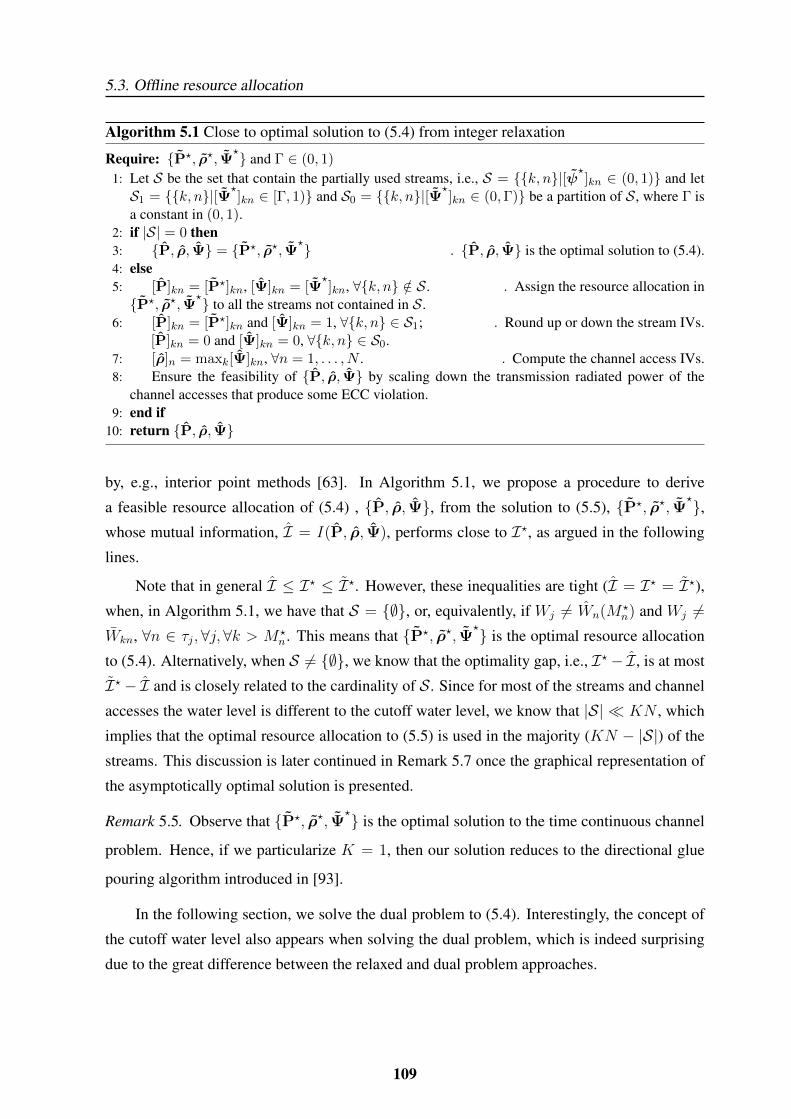
5.3. Offline resource allocation
Algorithm 5.1 Close to optimal solution to (5.4) from integer relaxation
Require: {P?, ρ?, Ψ?} and Γ ∈ (0, 1)
1: Let S be the set that contain the partially used streams, i.e., S = {{k, n}|[ψ?]kn ∈ (0, 1)} and letS1 = {{k, n}|[Ψ?
]kn ∈ [Γ, 1)} and S0 = {{k, n}|[Ψ?]kn ∈ (0,Γ)} be a partition of S, where Γ is
a constant in (0, 1).2: if |S| = 0 then3: {P, ρ, Ψ} = {P?, ρ?, Ψ
?} . {P, ρ, Ψ} is the optimal solution to (5.4).4: else5: [P]kn = [P?]kn, [Ψ]kn = [Ψ
?]kn, ∀{k, n} /∈ S. . Assign the resource allocation in
{P?, ρ?, Ψ?} to all the streams not contained in S.
6: [P]kn = [P?]kn and [Ψ]kn = 1, ∀{k, n} ∈ S1; . Round up or down the stream IVs.[P]kn = 0 and [Ψ]kn = 0, ∀{k, n} ∈ S0.
7: [ρ]n = maxk[Ψ]kn, ∀n = 1, . . . , N . . Compute the channel access IVs.8: Ensure the feasibility of {P, ρ, Ψ} by scaling down the transmission radiated power of the
channel accesses that produce some ECC violation.9: end if
10: return {P, ρ, Ψ}
by, e.g., interior point methods [63]. In Algorithm 5.1, we propose a procedure to derive
a feasible resource allocation of (5.4) , {P, ρ, Ψ}, from the solution to (5.5), {P?, ρ?, Ψ?},
whose mutual information, I = I(P, ρ, Ψ), performs close to I?, as argued in the following
lines.
Note that in general I ≤ I? ≤ I?. However, these inequalities are tight (I = I? = I?),when, in Algorithm 5.1, we have that S = {∅}, or, equivalently, if Wj 6= Wn(M?
n) and Wj 6=Wkn, ∀n ∈ τj,∀j,∀k > M?
n. This means that {P?, ρ?, Ψ?} is the optimal resource allocation
to (5.4). Alternatively, when S 6= {∅}, we know that the optimality gap, i.e., I?− I, is at most
I? − I and is closely related to the cardinality of S. Since for most of the streams and channel
accesses the water level is different to the cutoff water level, we know that |S| � KN , which
implies that the optimal resource allocation to (5.5) is used in the majority (KN − |S|) of the
streams. This discussion is later continued in Remark 5.7 once the graphical representation of
the asymptotically optimal solution is presented.
Remark 5.5. Observe that {P?, ρ?, Ψ?} is the optimal solution to the time continuous channel
problem. Hence, if we particularize K = 1, then our solution reduces to the directional glue
pouring algorithm introduced in [93].
In the following section, we solve the dual problem to (5.4). Interestingly, the concept of
the cutoff water level also appears when solving the dual problem, which is indeed surprising
due to the great difference between the relaxed and dual problem approaches.
109
Chapter 5. On the optimal resource allocation for a wireless energy harvesting nodeconsidering the circuitry power consumption
5.3.2 Duality
In this section, we study the Lagrange dual problem to (5.4) and show that, even though (5.4) is
not a convex optimization problem, the duality gap tends asymptotically to zero as the number
of streams or channel accesses per epoch grows without bound.
The Lagrangian of (5.4) is
L(P,ρ,Ψ,λ) = I(P,ρ,Ψ) + λTB(P,ρ,Ψ),
where λ = [λ1, . . . , λJ ]T is the dual variable that contains the Lagrange multipliers associated
with the ECCs. The dual function is defined for λ � 0 as
g(λ) = maximizeP,ρ,Ψ ∈ X
L(P,ρ,Ψ,λ)
(see [63]) and yields to upper bounds to the maximum achievable mutual information I? ob-
tained by maximizing the primal problem (5.4), i.e., I? ≤ g(λ). The Lagrange dual problem,
D? = minimizeλ�0
g(λ),
is a convex program that determines the best upper bound on I? as I? ≤ D? ≤ g(λ). The
duality gap is defined as D? − I? and it is zero if Slater qualification constraints are satisfied.
However, in our problem the Slater qualification constraints are not satisfied since the feasible
set X is not convex and, therefore, the duality gap might not be zero.
The time-sharing condition introduced in [119] provides a condition under which the du-
ality gap is zero even though the primal optimization problem is not convex. In the following
proposition, we demonstrate that the time-sharing condition is asymptotically satisfied as the
number of streams or channel accesses per epoch grows without bound.
Proposition 5.2. The time-sharing condition is asymptotically satisfied when, within each
epoch, every channel realization is observed a sufficiently large number of times.5
Proof: See Appendix 5.A.6.5The time sharing condition has been broadly used in different non-harvesting scenarios where the nodes
have to satisfy a single sum-power constraint. In such non-harvesting scenarios, the requirement for the asymptoticfulfillment of the time sharing condition is that every channel realization must be observed a large number of times[119]. When energy harvesting is considered, the problem is constrained by a set of ECCs and the time-sharingcondition is asymptotically satisfied if, within each epoch, every channel realization is observed a sufficientlylarge number of times. When K = 1, it is necessary that every channel realization is observed in a sufficientlylarge number of channel accesses. This situation happens, for instance, when the number of channel accesses perepoch is large, i.e., ej+1 − ej � 1, ∀j, and Tc � Ts. Whereas when K > 1, this condition is more likely to befulfilled due to the additional (space or frequency) dimension.
110
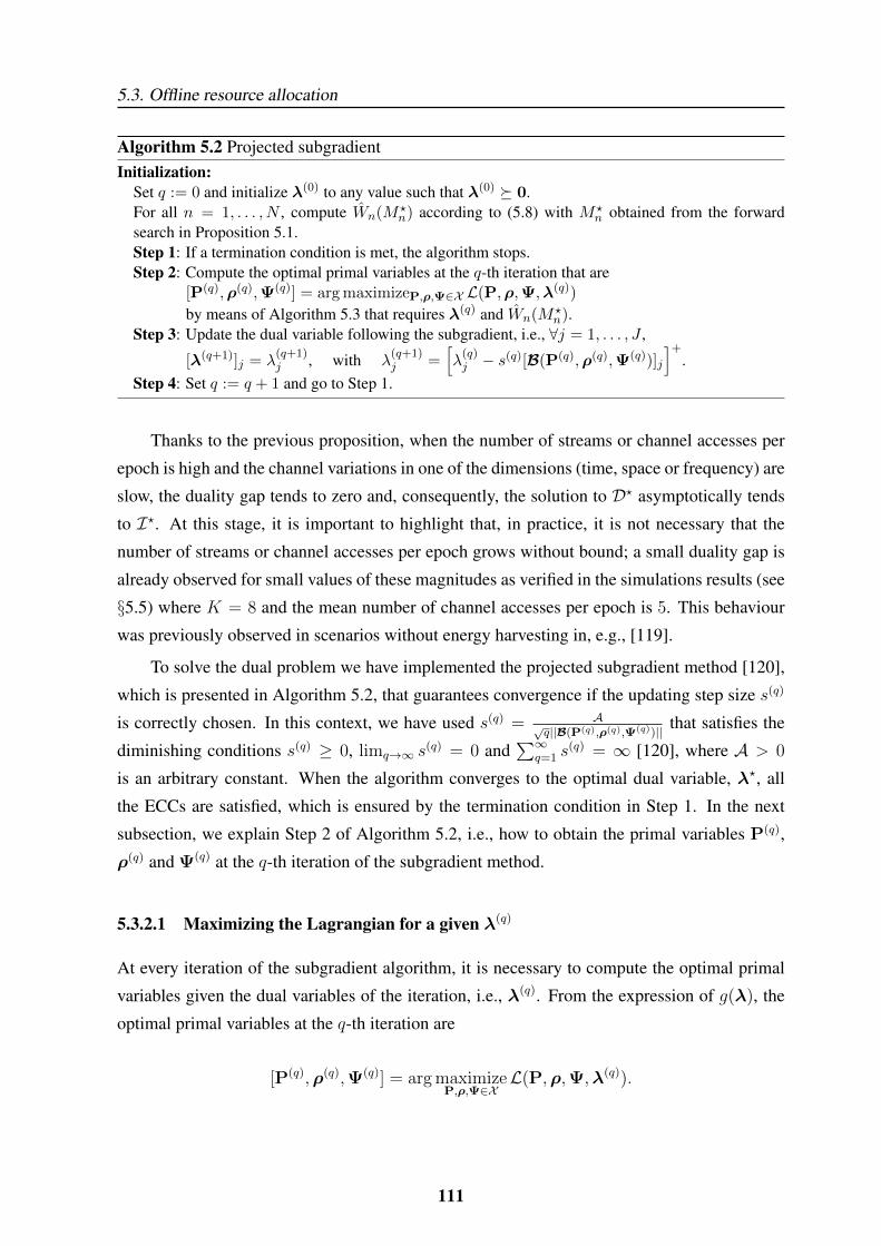
5.3. Offline resource allocation
Algorithm 5.2 Projected subgradientInitialization:
Set q := 0 and initialize λ(0) to any value such that λ(0) � 0.For all n = 1, . . . , N , compute Wn(M?
n) according to (5.8) with M?n obtained from the forward
search in Proposition 5.1.Step 1: If a termination condition is met, the algorithm stops.Step 2: Compute the optimal primal variables at the q-th iteration that are
[P(q),ρ(q),Ψ(q)] = arg maximizeP,ρ,Ψ∈X L(P,ρ,Ψ,λ(q))
by means of Algorithm 5.3 that requires λ(q) and Wn(M?n).
Step 3: Update the dual variable following the subgradient, i.e., ∀j = 1, . . . , J ,
[λ(q+1)]j = λ(q+1)j , with λ
(q+1)j =
[λ
(q)j − s(q)[B(P(q),ρ(q),Ψ(q))]j
]+.
Step 4: Set q := q + 1 and go to Step 1.
Thanks to the previous proposition, when the number of streams or channel accesses per
epoch is high and the channel variations in one of the dimensions (time, space or frequency) are
slow, the duality gap tends to zero and, consequently, the solution to D? asymptotically tends
to I?. At this stage, it is important to highlight that, in practice, it is not necessary that the
number of streams or channel accesses per epoch grows without bound; a small duality gap is
already observed for small values of these magnitudes as verified in the simulations results (see
§5.5) where K = 8 and the mean number of channel accesses per epoch is 5. This behaviour
was previously observed in scenarios without energy harvesting in, e.g., [119].
To solve the dual problem we have implemented the projected subgradient method [120],
which is presented in Algorithm 5.2, that guarantees convergence if the updating step size s(q)
is correctly chosen. In this context, we have used s(q) = A√q||B(P(q),ρ(q),Ψ(q))|| that satisfies the
diminishing conditions s(q) ≥ 0, limq→∞ s(q) = 0 and
∑∞q=1 s
(q) = ∞ [120], where A > 0
is an arbitrary constant. When the algorithm converges to the optimal dual variable, λ?, all
the ECCs are satisfied, which is ensured by the termination condition in Step 1. In the next
subsection, we explain Step 2 of Algorithm 5.2, i.e., how to obtain the primal variables P(q),
ρ(q) and Ψ(q) at the q-th iteration of the subgradient method.
5.3.2.1 Maximizing the Lagrangian for a given λ(q)
At every iteration of the subgradient algorithm, it is necessary to compute the optimal primal
variables given the dual variables of the iteration, i.e., λ(q). From the expression of g(λ), the
optimal primal variables at the q-th iteration are
[P(q),ρ(q),Ψ(q)] = arg maximizeP,ρ,Ψ∈X
L(P,ρ,Ψ,λ(q)).
111
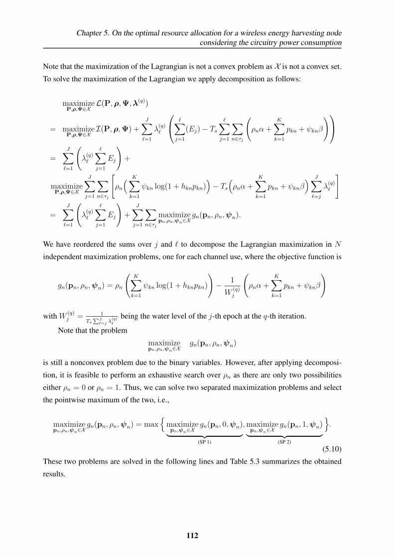
Chapter 5. On the optimal resource allocation for a wireless energy harvesting nodeconsidering the circuitry power consumption
Note that the maximization of the Lagrangian is not a convex problem as X is not a convex set.
To solve the maximization of the Lagrangian we apply decomposition as follows:
maximizeP,ρ,Ψ∈X
L(P,ρ,Ψ,λ(q))
= maximizeP,ρ,Ψ∈X
I(P,ρ,Ψ) +J∑`=1
λ(q)`
∑j=1
(Ej)− Ts∑j=1
∑n∈τj
(ρnα +
K∑k=1
pkn + ψknβ
)=
J∑`=1
(λ
(q)`
∑j=1
Ej
)+
maximizeP,ρ,Ψ∈X
J∑j=1
∑n∈τj
[ρn
( K∑k=1
ψkn log(1 + hknpkn))− Ts
(ρnα +
K∑k=1
pkn + ψknβ) J∑`=j
λ(q)`
]
=J∑`=1
(λ
(q)`
∑j=1
Ej
)+
J∑j=1
∑n∈τj
maximizepn,ρn,ψn∈X
gn(pn, ρn,ψn).
We have reordered the sums over j and ` to decompose the Lagrangian maximization in N
independent maximization problems, one for each channel use, where the objective function is
gn(pn, ρn,ψn) = ρn
(K∑k=1
ψkn log(1 + hknpkn)
)− 1
W(q)j
(ρnα +
K∑k=1
pkn + ψknβ
)
with W (q)j = 1
Ts∑J`=j λ
(q)`
being the water level of the j-th epoch at the q-th iteration.
Note that the problem
maximizepn,ρn,ψn∈X
gn(pn, ρn,ψn)
is still a nonconvex problem due to the binary variables. However, after applying decomposi-
tion, it is feasible to perform an exhaustive search over ρn as there are only two possibilities
either ρn = 0 or ρn = 1. Thus, we can solve two separated maximization problems and select
the pointwise maximum of the two, i.e.,
maximizepn,ρn,ψn∈X
gn(pn, ρn,ψn) = max{
maximizepn,ψn∈X
gn(pn, 0,ψn)︸ ︷︷ ︸(SP 1)
,maximizepn,ψn∈X
gn(pn, 1,ψn)︸ ︷︷ ︸(SP 2)
}.
(5.10)
These two problems are solved in the following lines and Table 5.3 summarizes the obtained
results.
112
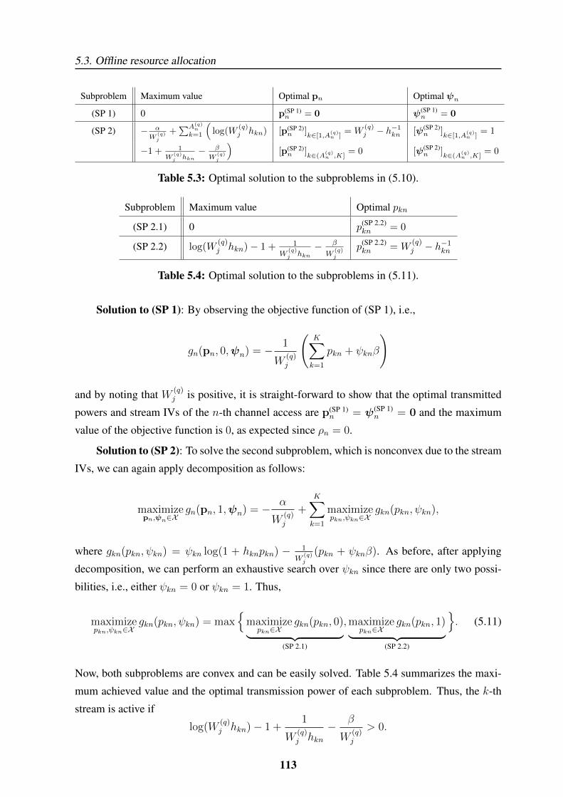
5.3. Offline resource allocation
Subproblem Maximum value Optimal pn Optimal ψn
(SP 1) 0 p(SP 1)n = 0 ψ(SP 1)
n = 0
(SP 2) − α
W(q)j
+∑A(q)
n
k=1
(log(W
(q)j hkn) [p(SP 2)
n ]k∈[1,A(q)
n ]= W
(q)j − h−1kn [ψ(SP 2)
n ]k∈[1,A(q)
n ]= 1
−1 + 1
W(q)j hkn
− β
W(q)j
)[p(SP 2)n ]
k∈(A(q)n ,K]
= 0 [ψ(SP 2)n ]
k∈(A(q)n ,K]
= 0
Table 5.3: Optimal solution to the subproblems in (5.10).
Subproblem Maximum value Optimal pkn
(SP 2.1) 0 p(SP 2.2)kn = 0
(SP 2.2) log(W(q)j hkn)− 1 + 1
W(q)j hkn
− β
W(q)j
p(SP 2.2)kn = W
(q)j − h−1
kn
Table 5.4: Optimal solution to the subproblems in (5.11).
Solution to (SP 1): By observing the objective function of (SP 1), i.e.,
gn(pn, 0,ψn) = − 1
W(q)j
(K∑k=1
pkn + ψknβ
)
and by noting that W (q)j is positive, it is straight-forward to show that the optimal transmitted
powers and stream IVs of the n-th channel access are p(SP 1)n = ψ(SP 1)
n = 0 and the maximum
value of the objective function is 0, as expected since ρn = 0.
Solution to (SP 2): To solve the second subproblem, which is nonconvex due to the stream
IVs, we can again apply decomposition as follows:
maximizepn,ψn∈X
gn(pn, 1,ψn) = − α
W(q)j
+K∑k=1
maximizepkn,ψkn∈X
gkn(pkn, ψkn),
where gkn(pkn, ψkn) = ψkn log(1 + hknpkn) − 1
W(q)j
(pkn + ψknβ). As before, after applying
decomposition, we can perform an exhaustive search over ψkn since there are only two possi-
bilities, i.e., either ψkn = 0 or ψkn = 1. Thus,
maximizepkn,ψkn∈X
gkn(pkn, ψkn) = max{
maximizepkn∈X
gkn(pkn, 0)︸ ︷︷ ︸(SP 2.1)
,maximizepkn∈X
gkn(pkn, 1)︸ ︷︷ ︸(SP 2.2)
}. (5.11)
Now, both subproblems are convex and can be easily solved. Table 5.4 summarizes the maxi-
mum achieved value and the optimal transmission power of each subproblem. Thus, the k-th
stream is active if
log(W(q)j hkn)− 1 +
1
W(q)j hkn
− β
W(q)j
> 0.
113
Chapter 5. On the optimal resource allocation for a wireless energy harvesting nodeconsidering the circuitry power consumption
Solving the previous equation (set M := 1, W := Wkn, H1 := hkn and Pc := β in Appendix
5.A.7), we obtain an equivalent condition for the k-th stream activation, i.e., W (q)j > Wkn,
where Wkn is the stream cutoff water level given in (5.9). Thus, after evaluating the condition
W(q)j > Wkn, ∀k, we obtain the number of streams that are activated if the channel access is
active, A(q)n .
Now that both (SP 1) and (SP 2) are solved (Table 5.3 summarizes the obtained results),
we can conclude that the n-th channel access is active if
− α
W(q)j
+
A(q)n∑
k=1
(log(W
(q)j hkn)− 1 +
1
W(q)j hkn
− β
W(q)j
)> 0
or, equivalently, if W (q)j > Wn(A
(q)n ) (set M := A
(q)n , W := Wn(A
(q)n ), Hk := hkn, and
Pc := A(q)n β + α in Appendix 5.A.7 to show this equivalence).6
In summary, the optimal primal variables at the q-th iteration of the subgradient can be
obtained by checking the condition W (q)j > Wkn, ∀k, to obtain the number of streams that
would be active if the channel access was active, A(q)n , and then checking the condition W (q)
j >
Wn(A(q)n ) to find out whether the channel access is active or not. If the channel access is active,
the optimal primal variables at the q-th iteration of the subgradient are p(q)n = p
(SP2)n , ψ(q)
n =
ψ(SP2)n , and ρ(q)
n = 1. Otherwise, we have that p(q)n = 0, ψ(q)
n = 0, and ρ(q)n = 0. However, this
procedure might be quite inefficient when the number of streams is large (K � 1) and it can
be avoided by first checking whether the channel access is active. Note that for any value of
A(q)n the channel access is active if and only if W (q)
j > Wn(M?n).7 In this context, the procedure
in Algorithm 5.3 is equivalent to the proposed above, but more computationally efficient.
Remark 5.6. The resource allocation obtained by solving the dual problem is almost equal to
the one obtained by means of the relaxed problem, which is given in Lemmas 5.1 and 5.2.
The channel access or stream activation conditions obtained in this section only differ from
the ones in Lemmas 5.1 and 5.2 when the water level is equal to the stream or channel access
cutoff water levels. In this section we have seen that if Wj = Wn(M?n) (or Wj = Wkn for
k ∈ (M?n, K]), it is indifferent to have the channel access (or stream) active or inactive since
both situations achieve the same value of the dual function, whereas, in the relaxed problem we
6Note that whenW (q)j = Wkn (orW (q)
j = Wn(A(q)n )) it is equivalent to activate or not the stream (or channel
access) since both achieve the same value of the objective function.7By using the definition of M?
n and Lemmas 5.3 and 5.4 in Appendix 5.A.3, it is easy to show that: ifA
(q)n > M?
n, then Wn(M?n) < Wn(A
(q)n ) < W
A(q)n ,n
< Wj ; and if A(q)n < M?
n, then Wn(A(q)n ) ≥ Wn(M?
n) ≥WM?
n,n≥Wj > W
A(q)n ,n
. Thus, from these inequalities, we can compareWj directly with Wn(M?n) to determine
whether the channel access is active or not.
114

5.3. Offline resource allocation
Algorithm 5.3 Maximization of the Lagrangian
Data: λ(q), Wn(M?n).
1: Compute W (q)j = 1
Ts∑J`=j λ
(q)`
, ∀j = 1, . . . , J . . Compute the water level in all the epochs given
λ(q).2: for n ∈ τj , j := 1, . . . , J do . For all the channel accesses.3: if W (q)
j > Wn(M?n) then . Check if the channel access is active.
4: A(q)n := M?
n; . The channel access is active; Then, count the number of active streams.5: for k := M?
n + 1, . . . ,K do6: if W (q)
j > Wkn then7: A
(q)n := A
(q)n + 1; . The k-th stream is active at the q-th iteration water level.
8: end if9: end for . End of counting.
10: p(q)n = p
(SP2)n , ψ(q)
n = ψ(SP2)n , and ρ(q)
n = 1;11: else12: p
(q)n = 0, ψ(q)
n = 0, and ρ(q)n = 0; . The n-th channel access is turned off.
13: end if14: end for
obtained that a partial use of the channel access (or the stream) is optimal, which is not allowed
in the problem considered in this section due to the binary feasible set of the IVs.
5.3.3 The Boxed Water-Flowing interpretation
In this section, we provide a graphical representation of the asymptotically optimal offline
solution named the Boxed Water-Flowing interpretation, which is depicted in Figure 5.2. This
interpretation follows directly from the concept of the cutoff water levels and it generalizes the
DWF interpretation in §2.3.1 [84] by considering the different sources of energy consumption
at the transmitter. The interpretation is the following:
(1.) Each stream is represented with a water-porous vessel with base equal to Ts.8 There
are two types of boxes, namely, the channel access box and the stream box. At the n-th
channel access, the channel access box with height Wn(M?n) is shared among the streams
k = 1, . . . ,M?n. The remaining streams, i.e., k > M?
n, have their own stream box with
height equal to Wkn.9 A water right-permeable material is used to separate the different
epochs.
(2.) Each box is filled by a solid substance up to a height equal to h−1kn and the boxes are closed
by a lid. The cost (in terms of water) of opening the channel access box is (α+M?nβ)Ts,
whereas, the cost of opening each stream box is βTs.8The vessel boundaries are not depicted in Figure 5.2 for the sake of simplicity.9Thus, the n-th channel access has K −M?
n stream boxes and one channel access box.
115

Chapter 5. On the optimal resource allocation for a wireless energy harvesting nodeconsidering the circuitry power consumption
(3.) The water level is progressively increased to all epochs at the same time by adding the
necessary amount of water to each epoch. The maximum amount of water that can be
externally added at some epoch is given by the epoch’s harvested energy (depicted with
the top-down arrows in Figure 5.2).10 When some epoch runs out of water, it uses water
that flows from previous epochs (if any is available) in order to continue increasing the
water level simultaneously. When the water level reaches the lid of some box, check if
there is enough available water (in the current and previous epochs) to pay the cost of
opening the lid and to fill in the whole box with water. If there is enough water, remove
the lid (which means that the amount of water associated with the lid opening cost is
lost), let the water fill the box and go back to Step 3; otherwise, keep the lid in the box
and go back to Step 3.
(4.) When all the available water has been poured, the optimal power allocation is found as
the amount of water in each of the vessels divided by Ts or, equivalently, as the height of
the water in each vessel, i.e., pkn = [Wj − h−1kn ]+.
Interestingly, by particularizing the Boxed Water-Flowing interpretation to the case in
which there is no circuitry consumption (α = 0 and β = 0), the heights of the boxes re-
duce to its minimum possible value, i.e., h−1kn , (set α = 0 and β = 0 in Lemmas 5.1 and 5.2)
and the DWF graphical interpretation in [84] is recovered, which has been presented in §2.3.1.
Remark 5.7. Having the graphical representation of the asymptotically optimal solution in
mind, it is easy to understand why its performance is close to I?. In the representation shown
in Figure 5.2, all the streams are using the optimal resource allocation to (5.5), except the sec-
ond stream of τ1. After solving the integer relaxation problem, we would have obtained that a
fractional use of this stream would be optimal. However, as this fractional use is not allowed
in a discrete channel model, we do not know where to optimally allocate the small remaining
energy in τ1. In summary, the following arguments justify why the optimality gap of the Boxed
Water-Flowing solution is small:
• As mentioned before, if the water level is different than the cutoff water level of all the
boxes (ρ?n ∈ {0, 1} and ψ?kn ∈ {0, 1}, ∀k, n), then the Boxed Water-Flowing solution is
optimal and the optimality gap is zero.
• Otherwise, when some stream or slot is partially used (ρ?n ∈ (0, 1) or ψ?kn ∈ (0, 1)), the
remaining energy in the epoch is very small and can be allocated in any of the active10The amount of water corresponds to energy, whereas, the water level, i.e., the height of the water, corresponds
to power.
116
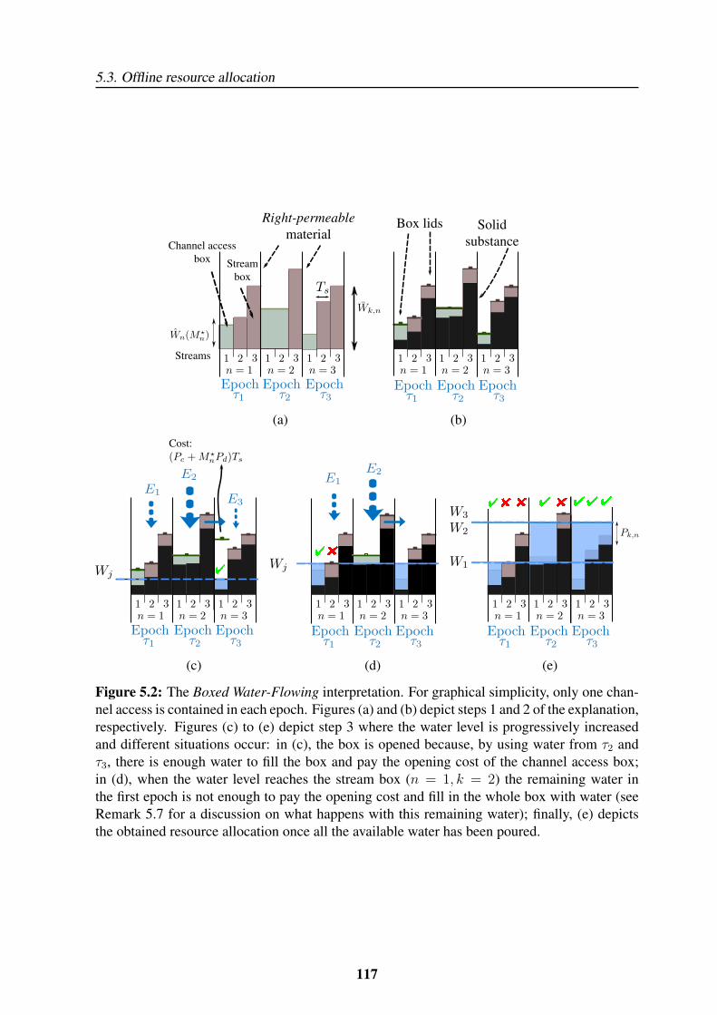
5.3. Offline resource allocation
Figure 5.2: The Boxed Water-Flowing interpretation. For graphical simplicity, only one chan-nel access is contained in each epoch. Figures (a) and (b) depict steps 1 and 2 of the explanation,respectively. Figures (c) to (e) depict step 3 where the water level is progressively increasedand different situations occur: in (c), the box is opened because, by using water from τ2 andτ3, there is enough water to fill the box and pay the opening cost of the channel access box;in (d), when the water level reaches the stream box (n = 1, k = 2) the remaining water inthe first epoch is not enough to pay the opening cost and fill in the whole box with water (seeRemark 5.7 for a discussion on what happens with this remaining water); finally, (e) depictsthe obtained resource allocation once all the available water has been poured.
117
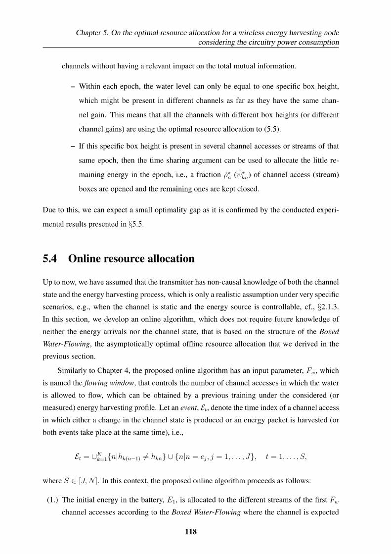
Chapter 5. On the optimal resource allocation for a wireless energy harvesting nodeconsidering the circuitry power consumption
channels without having a relevant impact on the total mutual information.
– Within each epoch, the water level can only be equal to one specific box height,
which might be present in different channels as far as they have the same chan-
nel gain. This means that all the channels with different box heights (or different
channel gains) are using the optimal resource allocation to (5.5).
– If this specific box height is present in several channel accesses or streams of that
same epoch, then the time sharing argument can be used to allocate the little re-
maining energy in the epoch, i.e., a fraction ρ?n (ψ?kn) of channel access (stream)
boxes are opened and the remaining ones are kept closed.
Due to this, we can expect a small optimality gap as it is confirmed by the conducted experi-
mental results presented in §5.5.
5.4 Online resource allocation
Up to now, we have assumed that the transmitter has non-causal knowledge of both the channel
state and the energy harvesting process, which is only a realistic assumption under very specific
scenarios, e.g., when the channel is static and the energy source is controllable, cf., §2.1.3.
In this section, we develop an online algorithm, which does not require future knowledge of
neither the energy arrivals nor the channel state, that is based on the structure of the Boxed
Water-Flowing, the asymptotically optimal offline resource allocation that we derived in the
previous section.
Similarly to Chapter 4, the proposed online algorithm has an input parameter, Fw, which
is named the flowing window, that controls the number of channel accesses in which the water
is allowed to flow, which can be obtained by a previous training under the considered (or
measured) energy harvesting profile. Let an event, Et, denote the time index of a channel access
in which either a change in the channel state is produced or an energy packet is harvested (or
both events take place at the same time), i.e.,
Et = ∪Kk=1{n|hk(n−1) 6= hkn} ∪ {n|n = ej, j = 1, . . . , J}, t = 1, . . . , S,
where S ∈ [J,N ]. In this context, the proposed online algorithm proceeds as follows:
(1.) The initial energy in the battery, E1, is allocated to the different streams of the first Fwchannel accesses according to the Boxed Water-Flowing where the channel is expected
118
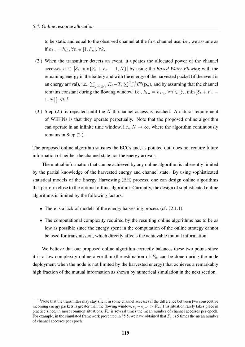
5.4. Online resource allocation
to be static and equal to the observed channel at the first channel use, i.e., we assume as
if hkn = hk1,∀n ∈ [1, Fw], ∀k.
(2.) When the transmitter detects an event, it updates the allocated power of the channel
accesses n ∈ [Et,min{Et + Fw − 1, N}] by using the Boxed Water-Flowing with the
remaining energy in the battery and with the energy of the harvested packet (if the event is
an energy arrival), i.e.,∑
j|ej≤Et Ej−Ts∑Et−1
n=1 C2(pn), and by assuming that the channel
remains constant during the flowing window, i.e., hkn = hkEt , ∀n ∈ [Et,min{Et + Fw −1, N}], ∀k.11
(3.) Step (2.) is repeated until the N -th channel access is reached. A natural requirement
of WEHNs is that they operate perpetually. Note that the proposed online algorithm
can operate in an infinite time window, i.e., N → ∞, where the algorithm continuously
remains in Step (2.).
The proposed online algorithm satisfies the ECCs and, as pointed out, does not require future
information of neither the channel state nor the energy arrivals.
The mutual information that can be achieved by any online algorithm is inherently limited
by the partial knowledge of the harvested energy and channel state. By using sophisticated
statistical models of the Energy Harvesting (EH) process, one can design online algorithms
that perform close to the optimal offline algorithm. Currently, the design of sophisticated online
algorithms is limited by the following factors:
• There is a lack of models of the energy harvesting process (cf. §2.1.1).
• The computational complexity required by the resulting online algorithms has to be as
low as possible since the energy spent in the computation of the online strategy cannot
be used for transmission, which directly affects the achievable mutual information.
We believe that our proposed online algorithm correctly balances these two points since
it is a low-complexity online algorithm (the estimation of Fw can be done during the node
deployment when the node is not limited by the harvested energy) that achieves a remarkably
high fraction of the mutual information as shown by numerical simulation in the next section.
11Note that the transmitter may stay silent in some channel accesses if the difference between two consecutiveincoming energy packets is greater than the flowing window, ej − ej−1 > Fw. This situation rarely takes place inpractice since, in most common situations, Fw is several times the mean number of channel accesses per epoch.For example, in the simulated framework presented in §5.5, we have obtained that Fw is 5 times the mean numberof channel accesses per epoch.
119
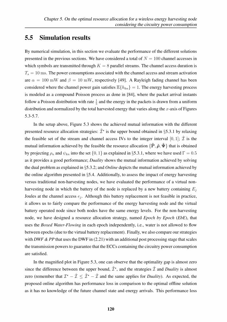
Chapter 5. On the optimal resource allocation for a wireless energy harvesting nodeconsidering the circuitry power consumption
5.5 Simulation results
By numerical simulation, in this section we evaluate the performance of the different solutions
presented in the previous sections. We have considered a total of N = 100 channel accesses in
which symbols are transmitted through K = 8 parallel streams. The channel access duration is
Ts = 10 ms. The power consumptions associated with the channel access and stream activation
are α = 100 mW and β = 10 mW, respectively [49]. A Rayleigh fading channel has been
considered where the channel power gain satisfies E{hkn} = 1. The energy harvesting process
is modeled as a compound Poisson process as done in [84], where the packet arrival instants
follow a Poisson distribution with rate 15
and the energy in the packets is drawn from a uniform
distribution and normalized by the total harvested energy that varies along the x-axis of Figures
5.3-5.7.
In the setup above, Figure 5.3 shows the achieved mutual information with the different
presented resource allocation strategies: I? is the upper bound obtained in §5.3.1 by relaxing
the feasible set of the stream and channel access IVs to the integer interval [0, 1]; I is the
mutual information achieved by the feasible the resource allocation {P, ρ, Ψ} that is obtained
by projecting ρn and ψkn into the set {0, 1} as explained in §5.3.1, where we have used Γ = 0.5
as it provides a good performance; Duality shows the mutual information achieved by solving
the dual problem as explained in §5.3.2; and Online depicts the mutual information achieved by
the online algorithm presented in §5.4. Additionally, to assess the impact of energy harvesting
versus traditional non-harvesting nodes, we have evaluated the performance of a virtual non-
harvesting node in which the battery of the node is replaced by a new battery containing EjJoules at the channel access ej . Although this battery replacement is not feasible in practice,
it allows us to fairly compare the performance of the energy harvesting node and the virtual
battery operated node since both nodes have the same energy levels. For the non-harvesting
node, we have designed a resource allocation strategy, named Epoch by Epoch (EbE), that
uses the Boxed Water-Flowing in each epoch independently, i.e., water is not allowed to flow
between epochs (due to the virtual battery replacement). Finally, we also compare our strategies
with DWF & PP that uses the DWF in (2.21) with an additional post processing stage that scales
the transmission powers to guarantee that the ECCs containing the circuitry power consumption
are satisfied.
In the magnified plot in Figure 5.3, one can observe that the optimality gap is almost zero
since the difference between the upper bound, I?, and the strategies I and Duality is almost
zero (remember that I? − I ≤ I? − I and the same applies for Duality). As expected, the
proposed online algorithm has performance loss in comparison to the optimal offline solution
as it has no knowledge of the future channel state and energy arrivals. This performance loss
120
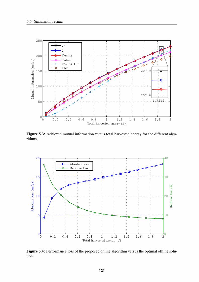
5.5. Simulation results
0 0.2 0.4 0.6 0.8 1 1.2 1.4 1.6 1.8 20
50
100
150
200
250
Total harvested energy (J)
Mutualinform
ation(nat/s)
I⋆
I
Duality
OnlineDWF & PPEbE
1.7214
207.6
207.9
Figure 5.3: Achieved mutual information versus total harvested energy for the different algo-rithms.
0 0.2 0.4 0.6 0.8 1 1.2 1.4 1.6 1.8 20
5
10
15
20
Absolute
loss
(nat/s)
Total harvested energy (J)
0 0.2 0.4 0.6 0.8 1 1.2 1.4 1.6 1.8 20
10
20
30
40
Relative
loss
(%)
Absolute lossRelative loss
Figure 5.4: Performance loss of the proposed online algorithm versus the optimal offline solu-tion.
121
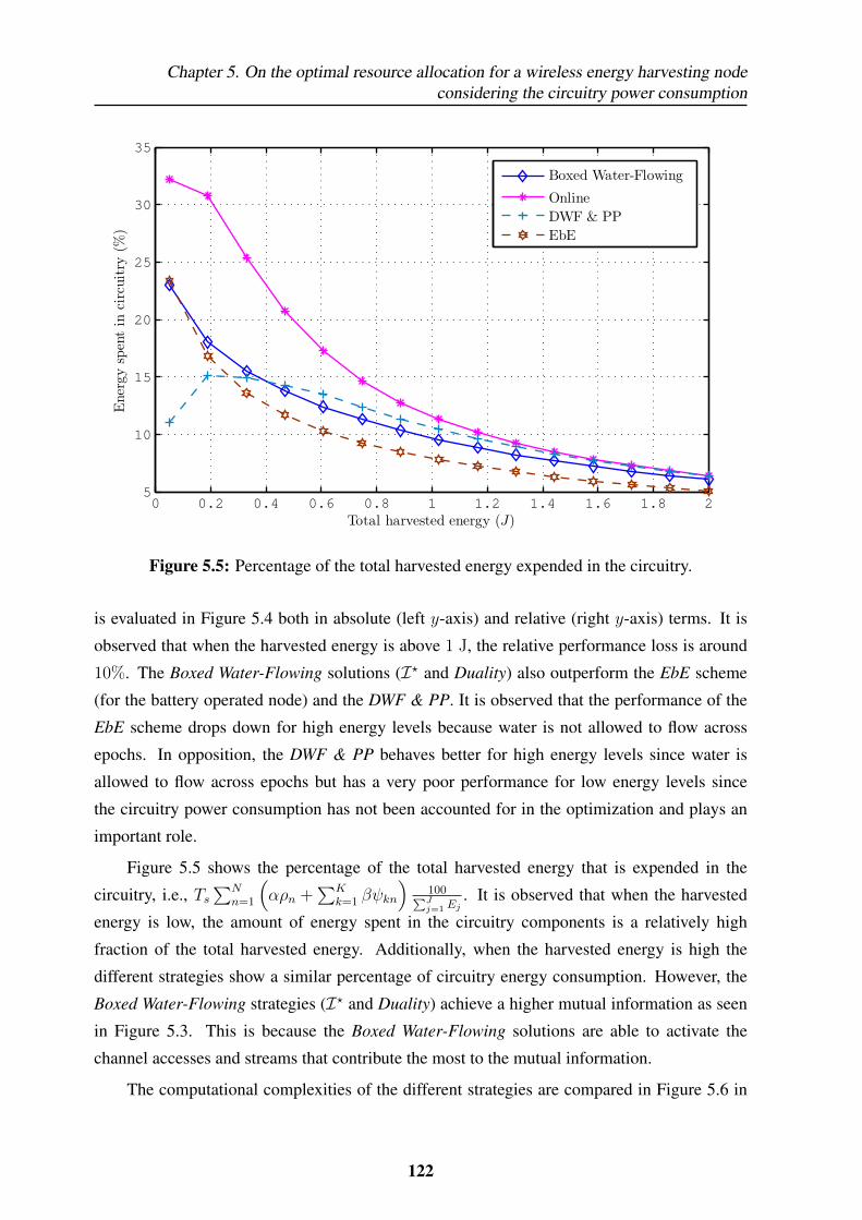
Chapter 5. On the optimal resource allocation for a wireless energy harvesting nodeconsidering the circuitry power consumption
0 0.2 0.4 0.6 0.8 1 1.2 1.4 1.6 1.8 25
10
15
20
25
30
35
Energyspentin
circuitry
(%)
Total harvested energy (J)
Boxed Water-Flowing
Online
DWF & PP
EbE
Figure 5.5: Percentage of the total harvested energy expended in the circuitry.
is evaluated in Figure 5.4 both in absolute (left y-axis) and relative (right y-axis) terms. It is
observed that when the harvested energy is above 1 J, the relative performance loss is around
10%. The Boxed Water-Flowing solutions (I? and Duality) also outperform the EbE scheme
(for the battery operated node) and the DWF & PP. It is observed that the performance of the
EbE scheme drops down for high energy levels because water is not allowed to flow across
epochs. In opposition, the DWF & PP behaves better for high energy levels since water is
allowed to flow across epochs but has a very poor performance for low energy levels since
the circuitry power consumption has not been accounted for in the optimization and plays an
important role.
Figure 5.5 shows the percentage of the total harvested energy that is expended in the
circuitry, i.e., Ts∑N
n=1
(αρn +
∑Kk=1 βψkn
)100∑Jj=1 Ej
. It is observed that when the harvested
energy is low, the amount of energy spent in the circuitry components is a relatively high
fraction of the total harvested energy. Additionally, when the harvested energy is high the
different strategies show a similar percentage of circuitry energy consumption. However, the
Boxed Water-Flowing strategies (I? and Duality) achieve a higher mutual information as seen
in Figure 5.3. This is because the Boxed Water-Flowing solutions are able to activate the
channel accesses and streams that contribute the most to the mutual information.
The computational complexities of the different strategies are compared in Figure 5.6 in
122
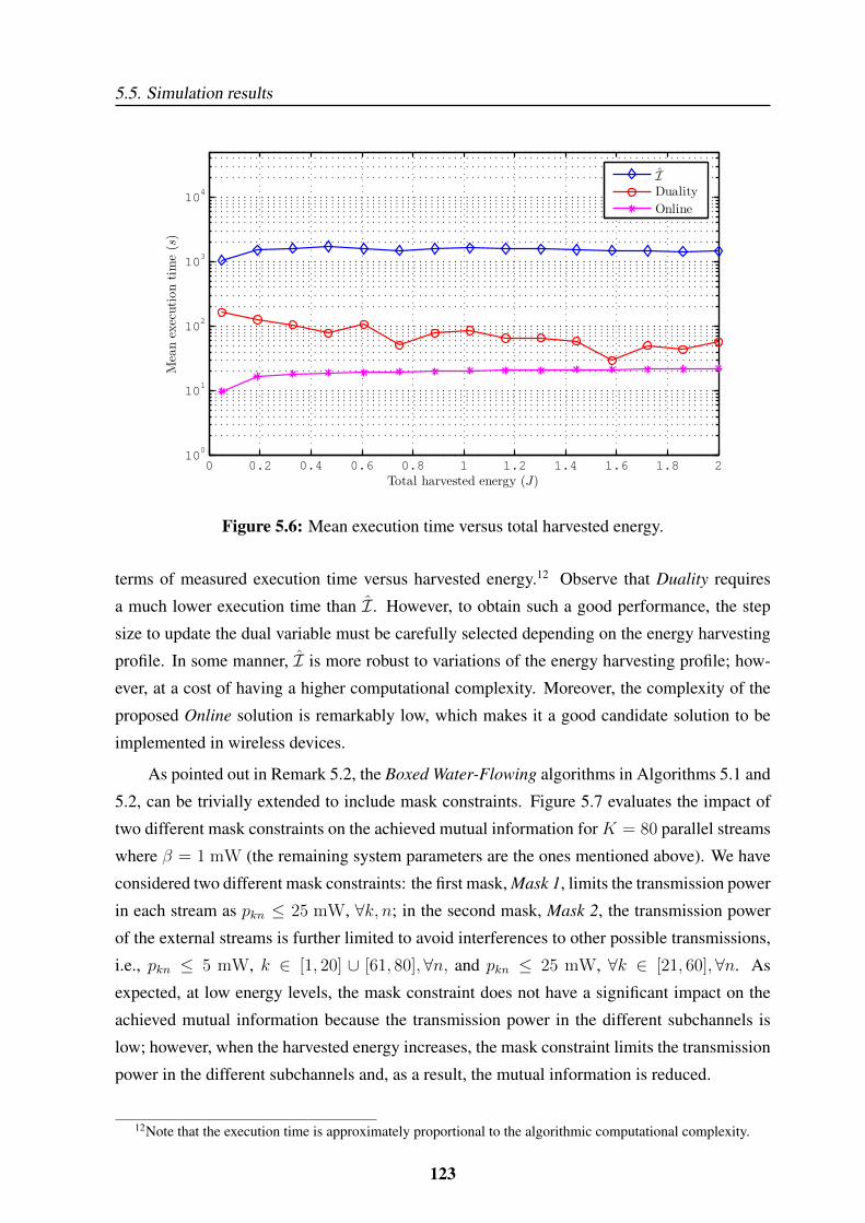
5.5. Simulation results
0 0.2 0.4 0.6 0.8 1 1.2 1.4 1.6 1.8 210
0
101
102
103
104
Total harvested energy (J)
Meanexecutiontime(s)
I
Duality
Online
Figure 5.6: Mean execution time versus total harvested energy.
terms of measured execution time versus harvested energy.12 Observe that Duality requires
a much lower execution time than I. However, to obtain such a good performance, the step
size to update the dual variable must be carefully selected depending on the energy harvesting
profile. In some manner, I is more robust to variations of the energy harvesting profile; how-
ever, at a cost of having a higher computational complexity. Moreover, the complexity of the
proposed Online solution is remarkably low, which makes it a good candidate solution to be
implemented in wireless devices.
As pointed out in Remark 5.2, the Boxed Water-Flowing algorithms in Algorithms 5.1 and
5.2, can be trivially extended to include mask constraints. Figure 5.7 evaluates the impact of
two different mask constraints on the achieved mutual information for K = 80 parallel streams
where β = 1 mW (the remaining system parameters are the ones mentioned above). We have
considered two different mask constraints: the first mask, Mask 1, limits the transmission power
in each stream as pkn ≤ 25 mW, ∀k, n; in the second mask, Mask 2, the transmission power
of the external streams is further limited to avoid interferences to other possible transmissions,
i.e., pkn ≤ 5 mW, k ∈ [1, 20] ∪ [61, 80],∀n, and pkn ≤ 25 mW, ∀k ∈ [21, 60],∀n. As
expected, at low energy levels, the mask constraint does not have a significant impact on the
achieved mutual information because the transmission power in the different subchannels is
low; however, when the harvested energy increases, the mask constraint limits the transmission
power in the different subchannels and, as a result, the mutual information is reduced.
12Note that the execution time is approximately proportional to the algorithmic computational complexity.
123
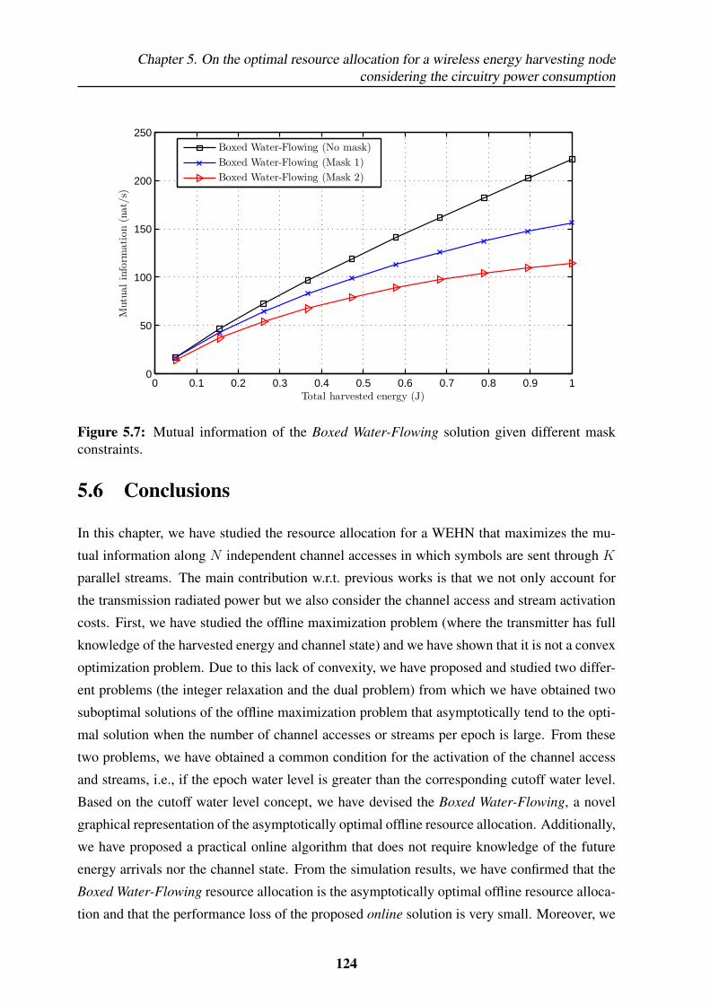
Chapter 5. On the optimal resource allocation for a wireless energy harvesting nodeconsidering the circuitry power consumption
0 0.1 0.2 0.3 0.4 0.5 0.6 0.7 0.8 0.9 10
50
100
150
200
250
Total harvested energy (J)
Mutualinform
ation(nat/s)
Boxed Water-Flowing (No mask)
Boxed Water-Flowing (Mask 1)
Boxed Water-Flowing (Mask 2)
Figure 5.7: Mutual information of the Boxed Water-Flowing solution given different maskconstraints.
5.6 Conclusions
In this chapter, we have studied the resource allocation for a WEHN that maximizes the mu-
tual information along N independent channel accesses in which symbols are sent through K
parallel streams. The main contribution w.r.t. previous works is that we not only account for
the transmission radiated power but we also consider the channel access and stream activation
costs. First, we have studied the offline maximization problem (where the transmitter has full
knowledge of the harvested energy and channel state) and we have shown that it is not a convex
optimization problem. Due to this lack of convexity, we have proposed and studied two differ-
ent problems (the integer relaxation and the dual problem) from which we have obtained two
suboptimal solutions of the offline maximization problem that asymptotically tend to the opti-
mal solution when the number of channel accesses or streams per epoch is large. From these
two problems, we have obtained a common condition for the activation of the channel access
and streams, i.e., if the epoch water level is greater than the corresponding cutoff water level.
Based on the cutoff water level concept, we have devised the Boxed Water-Flowing, a novel
graphical representation of the asymptotically optimal offline resource allocation. Additionally,
we have proposed a practical online algorithm that does not require knowledge of the future
energy arrivals nor the channel state. From the simulation results, we have confirmed that the
Boxed Water-Flowing resource allocation is the asymptotically optimal offline resource alloca-
tion and that the performance loss of the proposed online solution is very small. Moreover, we
124
5.A. Appendix
have evaluated the computational complexity of the different resource allocation strategies and
obtained that the online solution is the one that requires the lowest execution time.
5.A Appendix
5.A.1 Proof of Lemma 5.1
We know that the M?n streams that contribute to the channel access activation are the ones with
the best channel gains, i.e., h1n, . . . , hM?nn, because these streams are the ones that contribute
the most to the objective function. Given M?n, the following two conditions must be satisfied at
the cutoff water level, i.e., when Wj = Wn(M?n):
(C1) ∀k ≤ M?n, the following relations must be fulfilled: (i) pkn > 0; (ii) ψkn ∈ (0, 1); (iii)
ηkn = 0; (iv) ηkn = 0; and (v) ξkn = 0.13
(C2) ∀k > M?n, the following conditions must be satisfied: (i) pkn = 0; (ii) ψkn = 0; (iii)
ηkn = 0; and (iv) µkn = 0.14
Going back to (5.7), the radiated power of the streams k ≤ M?n at the channel access
cutoff water level is pkn = ψkn
(Wn(M?
n)− h−1kn
), where we have used that Wj = Wn(M?
n) =
(Ts∑J
`=j λ`)−1. Plugging this into the KKT condition in (5.6b), we have that all the streams
that contribute to the n-th channel access activation, i.e., k ≤M?n, must satisfy:
∂L∂ψkn
= log(hknWn(M?n))− 1 +
1
Wn(M?n)hkn
− β
Wn(M?n)− µkn = 0, ∀k ≤M?
n. (5.12)
Note that we cannot isolate Wn(M?n) in the previous equation due to the dependence on the
Lagrange multiplier µkn. To get rid of this dependence, we can use the KKT condition in
(5.6c) evaluated at the cutoff water level, i.e.,
K∑k=1
µkn =
M?n∑
k=1
µkn =α
Wn(M?n), (5.13)
where we have used that µkn = 0 ,∀k > M?n, which follows from (C2).
13Where (i) and (ii) follow from the fact that the stream must contribute to the channel access activation and(iii), (iv), and (v) follow from the slackness conditions (5.6f), (5.6g), and (5.6e), respectively.
14Where (i) and (ii) follow from the fact that the stream must not contribute to the channel access activationand (iii) and (iv) follow from the slackness conditions (5.6g) and (5.6h).
125
Chapter 5. On the optimal resource allocation for a wireless energy harvesting nodeconsidering the circuitry power consumption
With this, we can obtain an equation that does not depend on µkn by adding the equations∂L∂ψkn
= 0, ∀k ≤ M?n. Thus, the n-th channel access cutoff water level, Wn(M?
n), is obtained
by solving∑M?
nk=1
∂L∂ψkn
= 0, which is performed in Appendix 5.A.7 (set M := M?n, W :=
Wn(M?n), Hk := hkn, and Pc := M?
nβ + α), and is the one given in (5.8).
Up to now, we have shown that ifWj = Wn(M?n), the channel access is “partially on”, i.e.,
ρn ∈ (0, 1), ψkn ∈ (0, 1),∀k ≤ M?n and ψkn = 0,∀k > M?
n. Note that if Wj = Wn(M?n) + ε,
with ε > 0, then we have that log(hknWj) − 1 + 1Wjhkn
− βWj− µkn > 0. Thus, in order to
satisfy (5.6b), we must have ηkn > 0, ∀k ≤M?n. Then, from the slackness condition (5.6g), we
know that ψkn = 1, ∀k ≤M?n, and hence ρn = 1. A similar approach can be used to show that
if Wj < Wn(M?n), then ψkn = 0, ∀k, and hence ρn = 0.
5.A.2 Proof of Lemma 5.2
Now, we derive the expression of the k-th stream cutoff water level, Wkn, i.e., the water level at
which the k-th stream becomes partially active, where now k > M?n. Similarly as in the proof
of Lemma 5.1, in the k-th stream cutoff water level, we must have that pkn > 0, ψkn ∈ (0, 1),
ρn = 1, and from the slackness conditions we know that ηkn = 0, ηkn = 0, ξkn = 0, µkn = 0.
The k-th stream cutoff water level is obtained by solving the equation obtained from the KKT
condition in (5.6b) for Wkn (set M := 1, W := Wkn, H1 := hkn and Pc := β in Appendix
5.A.7) and is the one given in (5.9). Following the same procedure as in the last paragraph
of the proof of Lemma 5.1, it can be shown that if Wj > Wkn, k ∈ (M?n, K], then ψkn = 1.
Alternatively, if Wj < Wkn, k ∈ (M?n, K], then ψkn = 0.
5.A.3 Proof of Proposition 5.1
In this appendix, we prove that M?n can be found by performing a forward search over Mn
and that it is the smallest Mn that satisfies the condition Wn(Mn) < W(Mn+1)n. To prove
Proposition 5.1, we need to make use of the following two lemmas:
Lemma 5.3. If Wn(Mn) = W(Mn+1)n, then Wn(Mn + 1) = Wn(Mn).
Proof: See Appendix 5.A.4.
Lemma 5.4. If Wn(Mn) ≥ W(Mn+1)n, then: (a) Wn(Mn + 1) ≥ W(Mn+1)n; (b) the function
Wn(Mn + 1) is monotonically decreasing with h(Mn+1)n.
Proof: See Appendix 5.A.5.
126

5.A. Appendix
Observe that W(Mn+1)n is a function of h(Mn+1)n in opposition to Wn(Mn) that does not
depend on h(Mn+1)n. In this context, let h(Mn+1)n be the specific value of the channel gain of
the stream k = Mn + 1 that satisfies W(Mn+1)n = Wn(Mn).
We first show that any Mn smaller than M?n is suboptimal. We know that Wn(Mn) ≥
W(Mn+1)n, ∀Mn < M?n, since the condition Wn(Mn) < W(Mn+1)n is not satisfied until Mn :=
M?n. Since W(Mn+1)n is decreasing with the channel gain (see Remark 5.4), the condition
Wn(Mn) ≥ W(Mn+1)n implies h(Mn+1)n ≥ h(Mn+1)n. From Lemma 5.3, we have that at
h(Mn+1)n, Wn(Mn + 1) = Wn(Mn) and from Lemma 5.4.b if h(Mn+1)n ≥ h(Mn+1)n, then
Wn(Mn + 1) ≤ Wn(Mn), ∀Mn < M?n or, equivalently, Wn(1) ≥ Wn(2) ≥ · · · ≥ Wn(M?
n).
Therefore, any Mn in [1, M?n) is suboptimal.
Now, we prove the suboptimality of any Mn greater than M?n. From the structure of the
forward search, the following relationship is satisfied Wn(Mn) < W(Mn+1)n, ∀Mn ∈ [M?n, K].
Thus, the streams k > M?n cannot contribute to the channel access activation since these
streams are not active at the cutoff water level.
Finally, we must show that the streams k ≤ M?n are active in the channel access cutoff
water level, i.e., Wk,n ≤ Wn(M?n), which is verified as proved in Lemma 5.4.a.
5.A.4 Proof of Lemma 5.3
Let the channel access cutoff water level for a given Mn be expressed as
Wn(Mn) =XMn
1e(∏Mn
k=1 h1Mnkn )W0(XMn)
,
where XMn is the argument of the Lambert function, i.e.,
XMn =
∏Mn
k=1 h1Mnkn
eMn
(α +Mnβ −Mn∑k=1
h−1kn ). (5.14)
In the following lines, we impose the condition W(Mn+1)n = Wn(Mn), and, after some algebra,
we obtain the argument of the Lambert function in Wn(Mn + 1), i.e., XMn+1, where the tilde
denotes that W(Mn+1)n = Wn(Mn):
127
Chapter 5. On the optimal resource allocation for a wireless energy harvesting nodeconsidering the circuitry power consumption
(∏Mn
k=1 h1Mn
kn )W(Mn+1)n
elog
(∏Mn
k=1 h1Mn
kn )W(Mn+1)n
e
=
∏Mn
k=1 h1Mn
kn
eMn(α+Mnβ −
Mn∑k=1
h−1kn )⇒ (5.15)
XMn+1 =
∏Mn+1k=1 h
1Mn+1
kn
e(Mn + 1)
MnW(Mn+1)n log
(∏Mn
k=1 h1Mn
kn )W(Mn+1)n
e
+ β − h−1(Mn+1)n
⇒ (5.16)
XMn+1 =(∏Mn+1k=1 h
1Mn+1
kn )MnW(Mn+1)n
e(Mn + 1)
log
(∏Mn
k=1 h1Mn
kn )W(Mn+1)n
e
+W0(
βh(Mn+1)n−1e )
Mn
⇒ (5.17)
XMn+1 =(∏Mn+1k=1 h
1Mn+1
kn )W(Mn+1)n
e(Mn + 1)log
((∏Mn
k=1 hkn)WMn
(Mn+1)n
eMneW0(
βh(Mn+1)n−1
e )
)⇒ (5.18)
XMn+1 =(∏Mn+1k=1 h
1Mn+1
kn )W(Mn+1)n
elog
(∏Mn+1k=1 h
1Mn+1
kn )W(Mn+1)n
e
(5.19)
To obtain (5.16), we have multiplied both sides in (5.15) by Mn∏Mn+1k=1 h
1Mn+1kn∏Mn
k=1 h1Mnkn
and used the
definition of XMn+1, which follows from (5.14). In (5.19), we have used that eW(z) = zW(z)
,
which directly follows from the definition of the Lambert function.
The cutoff water level forMn+1 active streams is Wn(Mn+1) =XMn+1
1e
(∏Mn+1k=1 h
1Mn+1kn )W0(XMn+1)
,
from where
XMn+1 =
∏Mn+1k=1 h
1Mn+1
kn
eWn(Mn + 1) log
∏Mn+1k=1 h
1Mn+1
kn
eWn(Mn + 1)
.
By comparing this expression with (5.19), we have that Wn(Mn+1) must be equal to W(Mn+1)n
and, thus, we have Wn(Mn + 1) = Wn(Mn).
5.A.5 Proof of Lemma 5.4
5.A.5.1 Proof of Lemma 5.4.a
Following similar steps as in (5.15)-(5.19), it is easy to show that if Wn(Mn) ≥ W(Mn+1)n, then
XMn+1 ≥ XMn+1. From where, it follows XMn+1
W0(XMn+1)≥ (
∏Mn+1k=1 h
1Mn+1kn )W(Mn+1)n
eand, therefore,
we also have Wn(Mn + 1) ≥ W(Mn+1)n.
128
5.A. Appendix
5.A.5.2 Proof of Lemma 5.4.b
In the following lines, we demonstrate that ∂Wn(Mn+1)∂h(Mn+1)n
≤ 0 for Wn(Mn) ≥ W(Mn+1)n or, equiv-
alently, for XMn+1 ≥ XMn+1. Thus, we look at the sign of the derivative, sign[∂Wn(Mn+1)∂h(Mn+1)n
],
i.e.,
sign
[h−2(Mn+1)n
Mn + 1W0(XMn+1)− 1
Mn + 1
((Mn + 1)β + α−
Mn+1∑k=1
h−1kn
)dW0(XMn+1)
dXMn+1
∂XMn+1
∂h(Mn+1)n
](5.20)
= sign
W0(XMn+1)−XMn+1
1 +eh(Mn+1)nXMn+1∏Mn+1
k=1 h1
Mn+1
kn
dW0(XMn+1)
dXMn+1
(5.21)
= sign
[W0(XMn+1)−XMn+1 (1 +mXMn+1)
W0(XMn+1)
XMn+1(1 +W0(XMn+1))
](5.22)
= sign
[W0(XMn+1) (W0(XMn+1)−mXMn+1)
](5.23)
In (5.21), we have used that
∂XMn+1
∂h(Mn+1)n
=XMn+1
(Mn + 1)h(Mn+1)n
+
∏Mn+1k=1 h
1Mn+1
kn
e(Mn + 1)h2(Mn+1)n
.
In (5.22), we have defined m , eh(Mn+1)n
(∏Mn+1k=1 h
1Mn+1
kn
)−1
and evaluated the derivative of
the Lambert function, i.e.,
dW0(XMn+1)
dXMn+1
=W0(XMn+1)
XMn+1(1 +W0(XMn+1)).
From (5.23), we see that the sign of the derivative depends on the product of the Lambert
function (which is positive for XMn+1 > 0 and negative for XMn+1 < 0) and the difference
between the Lambert function and a line with slope m. To demonstrate that Wn(Mn + 1) is
monotonically decreasing with h(Mn+1)n for XMn+1 ≥ XMn+1, we must show that
W0(XMn+1)(a)< mXMn+1
(b)
≤ mXMn+1, ∀XMn+1 > max{0, XMn+1}, (5.24)
W0(XMn+1)(a)> mXMn+1
(b)
≥ mXMn+1, ∀XMn+1 < XMn+1 < 0, (5.25)
where m is an arbitrary constant. Observe that when m ≤ m, inequalities (b) in (5.24) and
(5.25) are satisfied. In the following lines, we propose a specific m that allows us to prove
inequalities in (a) and thus to demonstrate that Wn(Mn + 1) is monotonically decreasing with
129
Chapter 5. On the optimal resource allocation for a wireless energy harvesting nodeconsidering the circuitry power consumption
h(Mn+1)n.
Note that, by replacing m in (5.19), we obtain
XMn+1 =W(Mn+1)nh(Mn+1)n
mlog
(W(Mn+1)nh(Mn+1)n
m
).
From this relation, we can express m as a function of XMn+1, i.e.,
m = W(Mn+1)nh(Mn+1)nW0(XMn+1)
XMn+1
.
Note that W(Mn+1)nh(Mn+1)n ≥ 1 because W(Mn+1)n ∈ [h−1(Mn+1)n,∞) as pointed out in Remark
5.4. Thus, m ≥ W0(XMn+1)
XMn+1. Let m denote the minimum slope, i.e., m =
W0(XMn+1)
XMn+1. Since
m ≤ m the inequalities (b) in (5.24) and (5.25) are satisfied. Note that the Lambert function,
W0(XMn+1), and the line mXMn+1 cross both at the origin (XMn+1 = 0) and at the point
XMn+1 = XMn+1, i.e.,W0(XMn+1) = mXMn+1. Finally, by using the concavity of the positive
branch of the Lambert function [80] and these two crossing points, it is straight forward to show
that the inequalities (a) in (5.24) and (5.25) are satisfied. Thus, Wn(Mn + 1) is monotonically
decreasing with h(Mn+1)n.
5.A.6 Proof of Proposition 5.2
Let E1 and E2 be two different energy harvesting profiles, where the energy packet arrival in-
stants are the same but the amount of energy in the packets is different, and let{P?
E1,ρ?E1
,Ψ?E1
}and
{P?
E2,ρ?E2
,Ψ?E2
}be the associated optimal solutions to (5.4), respectively. Therefore,
showing that the time-sharing condition is fulfilled is equivalent to demonstrating that
I(P?θE1+(1−θ)E2
,ρ?θE1+(1−θ)E2,Ψ?
θE1+(1−θ)E2) ≥
I(PθE1+(1−θ)E2 ,ρθE1+(1−θ)E2,ΨθE1+(1−θ)E2) ≥
θI(P?E1,ρ?E1
,Ψ?E1
) + (1− θ)I(P?E2,ρ?E2
,Ψ?E2
)
where θ ∈ [0, 1],{P?θE1+(1−θ)E2
,ρ?θE1+(1−θ)E2,Ψ?
θE1+(1−θ)E2
}is the optimal resource alloca-
tion for an energy harvesting profile equal to θE1 +(1−θ)E2 and{PθE1+(1−θ)E2 ,ρθE1+(1−θ)E2
,
ΨθE1+(1−θ)E2
}is any feasible resource allocation.
130
5.A. Appendix
In the following lines, we construct a feasible resource allocation,
{PθE1+(1−θ)E2 ,ρθE1+(1−θ)E2
,ΨθE1+(1−θ)E2
},
that satisfies the time sharing condition in an epoch by epoch basis. In this context, since the
procedure is the same for all the epochs, we just explain how to obtain the resource allocation
of the streams contained in a generic epoch τj . Let u = 1, . . . ,U be an index used to indicate
the different channel realizations observed within the streams in τj . Thus, U is the number of
different channel realizations within the epoch. Let the set Su contain all the streams in τj that
have channel gain equal to hu, i.e., Su = {{k, n}|hkn = hu, n ∈ τj}. Ku denotes the cardinal-
ity of Su, which is a large number since, in the proposition statement, we have considered that
within each epoch every channel realization is observed a sufficiently large number of times. In
the following lines, we explain how to construct the resource allocation of the channel accesses
in Su. Since Ku is large, θ can be approximated as θ ≈ NuKu
, where Nu is an integer in the
interval [0, Ku]. Due to the nature of DWF, the power allocated by the optimal solution given
some energy harvesting profile is equal for all the streams in Su because when a certain channel
access is active, the transmission power in (2.21) only depends on the epoch water level and
on the channel gain. We construct the resource allocation in the streams in Su by assigning
the resource allocation in {[P?E1
]k′n′ , [ρ?E1
]n′ , [Ψ?E1
]k′n′} to Nu streams of Su and the resource
allocation in {[P?E2
]k′n′ , [ρ?E2
]n′ , [Ψ?E2
]k′n′} to the remainingKu−Nu streams, where {k′, n′} is
any stream contained in Su. This procedure is repeated for the different channel realizations to
obtain the resource allocation in all the streams of τj , then the total power consumption in τj is
equivalent to θ times the power consumption in τj given by{P?
E1,ρ?E1
,Ψ?E1
}and (1−θ) times
the power consumption in τj given by{P?
E2,ρ?E2
,Ψ?E2
}. After repeating this process for all
the epochs, the constructed resource allocation{PθE1+(1−θ)E2 ,ρθE1+(1−θ)E2
,ΨθE1+(1−θ)E2
}is
a feasible solution as the ECCs are satisfied and the obtained mutual information is θI(P?E1,
ρ?E1,Ψ?
E1) + (1 − θ)I(P?
E2,ρ?E2
,Ψ?E2
). Therefore, we have shown that the time-sharing con-
dition is satisfied.
131

Chapter 5. On the optimal resource allocation for a wireless energy harvesting nodeconsidering the circuitry power consumption
5.A.7 Derivation of the cutoff water level
In this appendix, we use a generic notation that serves us to derive both Wn(Mn) and Wkn.
Thus, W denotes the cutoff water level for the case of considering M active streams at the
cutoff region with gains Hk, k ∈ [1,M ], and when the circuitry power consumption is Pc.
Specifically, W is obtained by solving the equation∑M
k=1
[log(WHk)− 1 + 1
WHk
]− Pc
W= 0
as follows:
W
(M∏k=1
H1M
k
)[log
(W
M∏k=1
H1M
k
)− log e
]+
1
M
(M∏k=1
H1M
k
)(M∑k=1
H−1k
)− PcM
(M∏k=1
H1M
k
)= 0⇒ (5.26)
W∏Mk=1H
1M
k
elog
(W∏Mk=1H
1M
k
e
)=
∏Mk=1H
1M
k
Me(Pc −
M∑k=1
H−1k )⇒ (5.27)
W =Pc −
∑Mk=1H
−1k
MW0
(∏Mk=1H
1Mk
Me (Pc −∑Mk=1H
−1k )
) (5.28)
In (5.26), we have multiplied by WM
(∏Mk=1H
1Mk
). In (5.28), we have used that b log b = a ⇔
b = aW(a)
, which follows from the definition of the Lambert function [80]. Moreover, since
W > H−1k , ∀k = [1,M ], so that the streams are active in the cutoff region, the term b is always
greater than e−1 and, thus, the positive branch of the Lambert function, which is denoted by
W0(·), is used.
132
Chapter 6Sum-rate maximization in multiuser
communications with WEHNs considering a
generalized power consumption model
6.1 Introduction
In the previous chapter, we have seen that it is key that the power consumption model accounts
not only for the transmission radiated power but also for the remaining energy sinks, which can
be modeled, in general, by step functions. As a result of considering the channel access and
stream activation costs, the (asymptotically) optimal transmission strategy alternates between
“off” and “on” cycles.
The power consumption model considered in the previous chapter, C2 in (5.1), is a good
first step towards the design of more efficient transmission strategies; however, still many
sources of energy consumption escape from the model, which must be progressively included
in the design. For example, “off-on” transitions also entail energy consumption due to the
startup time of the transceiver [51, 121] that can be taken into account by refining the power
133
Chapter 6. Sum-rate maximization in multiuser communications with WEHNs considering ageneralized power consumption model
consumption model C2 as:
C3n(pn,pn+1) =
C2(pn) if n = N ,
C2(pn) + γ
(1−H`
(K∑k=1
pkn
))H`
(K∑k=1
pk(n+1)
)︸ ︷︷ ︸
Startup power consumption
if n = 1, . . . , N − 1,
(6.1)
where γ ≥ 0 is the mean startup power consumption of the transceiver;(
1−H`(∑K
k=1 pkn
))is one when the n-th channel access is “off”, H`
(∑Kk=1 pk(n+1)
)is one when the (n + 1)-th
channel access is “on”, and their product takes value one when an “off-on” transition occurs.
Note that now the power consumption model depends on the channel access index, n, since the
last channel access cannot incur on startup power consumption.
Additionally, in the previous chapter, we have seen that when the power consumption
model includes step functions, the linear transmitter design is a nonconvex nonsmooth problem
since the ECCs are no longer linear (as occurs when solely the transmission radiated power is
considered, e.g., in DWF, cf. §2.3.1). Therefore, the optimal transmission strategy cannot
be found with classical convex optimization techniques. To overcome the nonconvexity of the
problem, in the previous chapter we have replaced the step functions by additional optimization
variables, named IVs, which has allowed us to derive an asymptotically optimal solution of the
problem.
The main advantages of reformulating the problem with IVs are:
(A1) Although the resulting problem is nonconvex (due to the presence of the binary IVs), by
integer relaxation, dual decomposition, or other techniques, one might obtain a convex
problem that performs close to the optimal solution as occurs in Chapter 5.
(A2) When the resulting problem is analytically tractable, one can obtain an intuition of the
structure of the solution as it has been shown with the Boxed Water-Flowing.
Nevertheless, the approach based on IVs also has the following inconveniences:
(I1) The computational complexity of the problem increases due to the additional number of
optimization variables.
(I2) In many transmitter designs, as the one explored in this chapter, even after perform-
ing integer relaxation of the IVs, the problem is still nonconvex; accordingly, for such
134

6.1. Introduction
problems, the use of IVs does not seem the best approach to obtain a good transmission
strategy.
(I3) It is generally difficult to deal with products of step functions in the power consumption
model since products of optimization variables are nonconvex even after integer relax-
ation, which leads to (I2); accordingly, it would be difficult to derive good solutions given
the power consumption model C3n in (6.1).
(I4) It is not robust to variations on the power consumption model, i.e., one must formulate
and solve an optimization problem for every single variation of the power consumption
model and, as we have seen in Chapter 5, finding the solution to the problem might be
indeed involved.
In this context, in the current chapter we propose an alternative approach for solving power
allocation problems that contain step functions; the proposed approach performs a successive
approximation of the step functions by smooth functions in order to derive a smooth nonconvex
optimization problem that can be solved by SCA [67]. The main advantages of this approach
w.r.t. the use of IVs are:
• It applies to nonconvex optimization problems.
• It accepts products of step functions, which allows us to take into account, among others,
the startup power consumption.
• It can be easily adapted to include new sources of energy consumption.
• The problem can be solved in a distributed way under very mild assumptions.
• In some applications, it provides a faster convergence due to the lower dimensionality of
the problem.
More precisely, in this chapter, we consider a network of WEHNs transmitting simulta-
neously in a Gaussian interference channel and investigate a distributed power allocation algo-
rithm that maximizes the sum-rate by considering a general power consumption model, which
is composed of step functions and permits to take into account the different sources of energy
consumption at each transmitter (e.g., the energy spent in the different components of the RF
chain when the transmitter is “on” or the startup power consumption).
135

Chapter 6. Sum-rate maximization in multiuser communications with WEHNs considering ageneralized power consumption model
To the best of our knowledge, a few works have considered the interference channel for
WEHNs: the authors of [114] assumed that the radiated power is the unique energy sink and
derived a policy that maximizes the sum-rate; whereas, the two-user Gaussian interference
channel was studied in [115] by considering the cost of having the transmitter “on”.
The major contributions of this chapter are:
• Proposing a smooth approximation of the step function in (2.6) that can be easily con-
vexified by state of the art SCA algorithms.
• Studying the power allocation strategy that maximizes the sum-rate in a network of en-
ergy harvesting nodes, which transmit simultaneously over a shared channel, by consid-
ering a generalized power consumption model that accepts products of step functions.
• Proposing the Iterative Smooth and Convex approximation Algorithm (ISCA), which
distributedly computes a stationary solution of the aforementioned problem.
The remainder of the chapter is structured as follows. In §6.2, the sum-rate maximization
problem for a network of WEHN is formulated. In §6.3, the smooth and convex approximations
of the step functions are given. In §6.4, the ISCA is presented for a general power consumption
model, which is particularized in §6.5 to the power consumption model C2 in (5.1). The per-
formance of the ISCA in terms of achieved rate and computational complexity is numerically
evaluated in §6.6. Finally, the chapter is concluded in §6.7.
6.2 System model and problem formulation
In the remaining of the chapter, we use the same notation as in the previous chapters with the
only difference that we use the subindex t to differentiate between the different transmitters.
We consider a Gaussian interference channel composed of T transmitter and receiver pairs
sharing the same band over SISO frequency-selective links composed ofK parallel subcarriers.
Transmission takes place during N time slots of duration Ts where, at the n-th slot, the channel
power gain from transmitter t to receiver r at the k-th subcarrier is denoted by htr(k, n). We
do not consider interference cancellation techniques in order to avoid the need of having a
centralized control or coordination in the network. Accordingly, we treat the MUI as additive
colored noise. Thus, assuming that Gaussian signaling is used, the rate of user t depends on
136
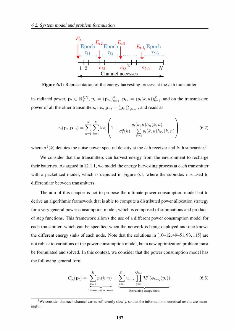
6.2. System model and problem formulation
Figure 6.1: Representation of the energy harvesting process at the t-th transmitter.
its radiated power, pt ∈ RKN+ , pt = (ptn)Nn=1 ,ptn = (pt(k, n))Kk=1, and on the transmission
power of all the other transmitters, i.e., p−t = (pt′)Tt′ 6=t=1, and reads as
rt(pt,p−t) =N∑n=1
K∑k=1
log
1 +pt(k, n)htt(k, n)
σ2t (k) +
∑t′ 6=t
pt(k, n)ht′t(k, n)
, (6.2)
where σ2t (k) denotes the noise power spectral density at the t-th receiver and k-th subcarrier.1
We consider that the transmitters can harvest energy from the environment to recharge
their batteries. As argued in §2.1.1, we model the energy harvesting process at each transmitter
with a packetized model, which is depicted in Figure 6.1, where the subindex t is used to
differentiate between transmitters.
The aim of this chapter is not to propose the ultimate power consumption model but to
derive an algorithmic framework that is able to compute a distributed power allocation strategy
for a very general power consumption model, which is composed of summations and products
of step functions. This framework allows the use of a different power consumption model for
each transmitter, which can be specified when the network is being deployed and one knows
the different energy sinks of each node. Note that the solutions in [10–12, 49–51, 93, 115] are
not robust to variations of the power consumption model, but a new optimization problem must
be formulated and solved. In this context, we consider that the power consumption model has
the following general form
C4tn(pt) =
K∑k=1
pt(k, n)︸ ︷︷ ︸Transmission power
+Stn∑s=1
wtns
Qtns∏q=1
H` (φtnsq(pt))︸ ︷︷ ︸Remaining energy sinks
, (6.3)
1We consider that each channel varies sufficiently slowly, so that the information theoretical results are mean-ingful.
137
Chapter 6. Sum-rate maximization in multiuser communications with WEHNs considering ageneralized power consumption model
where the subindex t and n denote a specific transmitter and channel access, respectively;
wtns 6= 0 is a given set of weights; Stn and Qtns ∈ N; and φtnsq : RK+ → R+ must be concave,
Lipschitz continuous, and continuously differentiable.
Since the different transmitters may have different architectures, they may also experience
different consumptions for the channel access/slot activation costs and startup of the transceiver.
Accordingly, we index the power consumption models C2 in (5.1) and C3n in (6.1) with an
additional index to distinguish between transmitters. Thus, we have
C2t (ptn) =
K∑k=1
pt(k, n)︸ ︷︷ ︸Transmission power
+ αtH`
(K∑k=1
pt(k, n)
)︸ ︷︷ ︸
Power consumption per active slot
+K∑k=1
βtH` (pt(k, n)) ,︸ ︷︷ ︸Power consumption per active stream
(6.4)
and C3tn(ptn,pt(n+1)) =
C2t (ptn) if n = N ,
C2t (ptn) + γt
(1−H`
(K∑k=1
pt(k, n)
))H`
(K∑k=1
pt(k, n+ 1)
)︸ ︷︷ ︸
Startup power consumption
if n = 1, . . . , N − 1,
(6.5)
respectively.
Note that C2t and C3
tn are particular cases of C4tn in (6.3); the associated weights and inner
functions, φtnsq(pt), are given in Table 6.1.
Our objective is to design a distributed power allocation strategy that maximizes the sum-
rate under an offline approach (cf. §2.1.3), i.e., by assuming that we have non-causal knowledge
of the channel gains and energy harvesting process. As argued in §2.1.3, this knowledge is
available when the channel is time-static and the power harvesting profile is controllable or
predictable, which happens, for example, with a solar harvester. Note that if a distributed power
allocation strategy is derived, then the nodes can recompute the solution when a substantial
change in the power profile prediction is observed. In non-static scenarios, the offline power
allocation is still useful because it can be used as a benchmark for the design and evaluation
of online transmission strategies, which does not require future knowledge of the harvested
energy and channel state.
In this context, the offline sum-rate maximization problem is
138
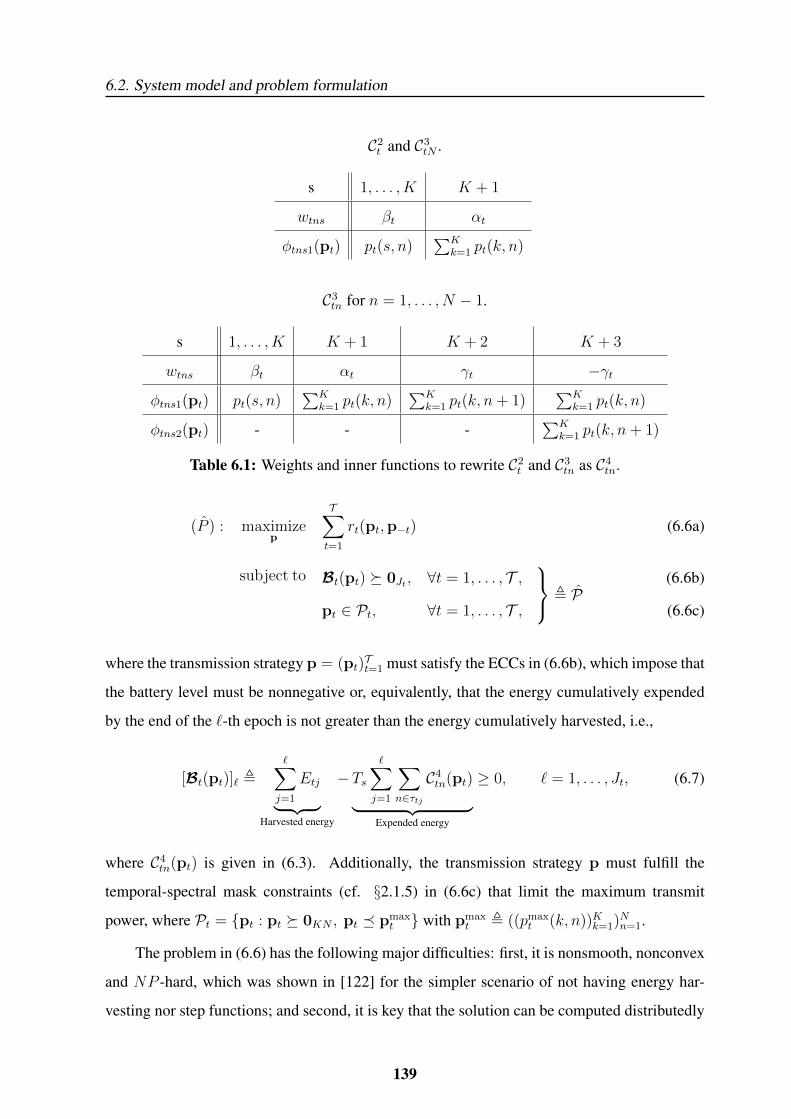
6.2. System model and problem formulation
C2t and C3
tN .
s 1, . . . , K K + 1
wtns βt αt
φtns1(pt) pt(s, n)∑K
k=1 pt(k, n)
C3tn for n = 1, . . . , N − 1.
s 1, . . . , K K + 1 K + 2 K + 3
wtns βt αt γt −γtφtns1(pt) pt(s, n)
∑Kk=1 pt(k, n)
∑Kk=1 pt(k, n+ 1)
∑Kk=1 pt(k, n)
φtns2(pt) - - -∑K
k=1 pt(k, n+ 1)
Table 6.1: Weights and inner functions to rewrite C2t and C3
tn as C4tn.
(P ) : maximizep
T∑t=1
rt(pt,p−t) (6.6a)
subject to , P
Bt(pt) � 0Jt , ∀t = 1, . . . , T , (6.6b)
pt ∈ Pt, ∀t = 1, . . . , T , (6.6c)
where the transmission strategy p = (pt)Tt=1 must satisfy the ECCs in (6.6b), which impose that
the battery level must be nonnegative or, equivalently, that the energy cumulatively expended
by the end of the `-th epoch is not greater than the energy cumulatively harvested, i.e.,
[Bt(pt)]` ,∑j=1
Etj︸ ︷︷ ︸Harvested energy
−Ts∑j=1
∑n∈τtj
C4tn(pt)︸ ︷︷ ︸
Expended energy
≥ 0, ` = 1, . . . , Jt, (6.7)
where C4tn(pt) is given in (6.3). Additionally, the transmission strategy p must fulfill the
temporal-spectral mask constraints (cf. §2.1.5) in (6.6c) that limit the maximum transmit
power, where Pt = {pt : pt � 0KN , pt � pmaxt } with pmax
t , ((pmaxt (k, n))Kk=1)Nn=1.
The problem in (6.6) has the following major difficulties: first, it is nonsmooth, nonconvex
and NP -hard, which was shown in [122] for the simpler scenario of not having energy har-
vesting nor step functions; and second, it is key that the solution can be computed distributedly
139
Chapter 6. Sum-rate maximization in multiuser communications with WEHNs considering ageneralized power consumption model
by the network nodes because then they can adjust their strategies when strong variations of
the energy harvesting profile are observed. In this context, we propose the ISCA that is able
to compute a distributed power allocation strategy that aims at maximizing the sum-rate. The
details of the ISCA are presented in §6.4. By now, it is important to know that it is composed
of two loops: the outer loop performs a SSA of the step functions to derive, at each iteration,
a smooth nonconvex problem that approximates (6.6); then, the inner loop solves this smooth
nonconvex problem by means of the SCA algorithm in [67].
In the following section, we introduce a smooth approximation of the step function that
can be easily convexified by SCA algorithms.
6.3 Approximations of the step function
The objective of this section is two-fold: (i) to design a smooth approximation of the unit step
function in (2.6), which is used in the outer loop of the ISCA; and (ii) to derive a convex ap-
proximation of the smooth approximation in (i) that can be handled by the SCA algorithm in
the inner loop. The later approximation, (ii), has to satisfy some tight requirements in order
to guarantee convergence [67], which are listed in [67, Assumption 3], that intrinsically cou-
ple the design of the approximations in (i) and (ii) because depending on the chosen smooth
approximation, it might be either easy or extremely difficult to later find an accurate convex
approximation. In this context, we can easily derive a convex approximation if the smooth
approximation is:
(C1) Differentiable.
(C2) An addition of concave and convex functions.
6.3.1 Smooth approximation of the step function
In this section, we present a smooth approximation of the step function that satisfies (C1)-(C2);
whereas, in §6.3.2, we present its convexification that satisfies [67, Assumption 3].
140
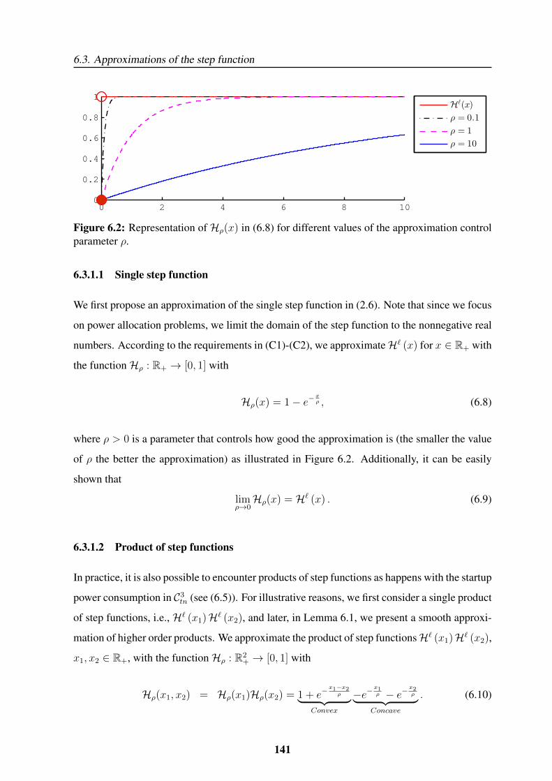
6.3. Approximations of the step function
0 2 4 6 8 100
0.2
0.4
0.6
0.8
1
Hℓ(x)
ρ = 0.1
ρ = 1
ρ = 10
Figure 6.2: Representation of Hρ(x) in (6.8) for different values of the approximation controlparameter ρ.
6.3.1.1 Single step function
We first propose an approximation of the single step function in (2.6). Note that since we focus
on power allocation problems, we limit the domain of the step function to the nonnegative real
numbers. According to the requirements in (C1)-(C2), we approximateH` (x) for x ∈ R+ with
the functionHρ : R+ → [0, 1] with
Hρ(x) = 1− e−xρ , (6.8)
where ρ > 0 is a parameter that controls how good the approximation is (the smaller the value
of ρ the better the approximation) as illustrated in Figure 6.2. Additionally, it can be easily
shown that
limρ→0Hρ(x) = H` (x) . (6.9)
6.3.1.2 Product of step functions
In practice, it is also possible to encounter products of step functions as happens with the startup
power consumption in C3tn (see (6.5)). For illustrative reasons, we first consider a single product
of step functions, i.e., H` (x1)H` (x2), and later, in Lemma 6.1, we present a smooth approxi-
mation of higher order products. We approximate the product of step functionsH` (x1)H` (x2),
x1, x2 ∈ R+, with the functionHρ : R2+ → [0, 1] with
Hρ(x1, x2) = Hρ(x1)Hρ(x2) = 1 + e−x1−x2ρ︸ ︷︷ ︸
Convex
−e−x1ρ − e−
x2ρ︸ ︷︷ ︸
Concave
. (6.10)
141
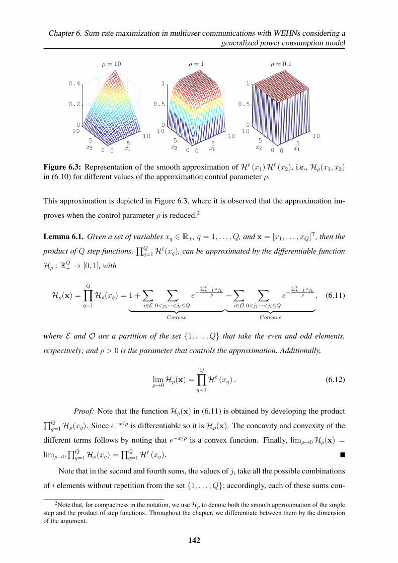
Chapter 6. Sum-rate maximization in multiuser communications with WEHNs considering ageneralized power consumption model
05
10
0
5
100
0.2
0.4
x1
ρ = 10
x2 05
10
0
5
100
0.5
1
x1
ρ = 1
x2 05
10
0
5
100
0.5
1
x1
ρ = 0.1
x2
Figure 6.3: Representation of the smooth approximation of H` (x1)H` (x2), i.e., Hρ(x1, x2)in (6.10) for different values of the approximation control parameter ρ.
This approximation is depicted in Figure 6.3, where it is observed that the approximation im-
proves when the control parameter ρ is reduced.2
Lemma 6.1. Given a set of variables xq ∈ R+, q = 1, . . . , Q, and x = [x1, . . . , xQ]T, then the
product of Q step functions,∏Q
q=1H`(xq), can be approximated by the differentiable function
Hρ : RQ+ → [0, 1], with
Hρ(x) =
Q∏q=1
Hρ(xq) = 1 +∑i∈E
∑0<j1···<ji≤Q
e−∑ik=1 xjkρ
︸ ︷︷ ︸Convex
−∑i∈O
∑0<j1···<ji≤Q
e−∑ik=1 xjkρ
︸ ︷︷ ︸Concave
, (6.11)
where E and O are a partition of the set {1, . . . , Q} that take the even and odd elements,
respectively; and ρ > 0 is the parameter that controls the approximation. Additionally,
limρ→0Hρ(x) =
Q∏q=1
H` (xq) . (6.12)
Proof: Note that the function Hρ(x) in (6.11) is obtained by developing the product∏Qq=1Hρ(xq). Since e−x/ρ is differentiable so it is Hρ(x). The concavity and convexity of the
different terms follows by noting that e−x/ρ is a convex function. Finally, limρ→0Hρ(x) =
limρ→0
∏Qq=1Hρ(xq) =
∏Qq=1H` (xq).
Note that in the second and fourth sums, the values of ji take all the possible combinations
of i elements without repetition from the set {1, . . . , Q}; accordingly, each of these sums con-
2Note that, for compactness in the notation, we useHρ to denote both the smooth approximation of the singlestep and the product of step functions. Throughout the chapter, we differentiate between them by the dimensionof the argument.
142
6.3. Approximations of the step function
tains Q!i!(Q−i!) summands. Observe that if we particularize the approximation in Lemma 6.1 to
Q = 1 and Q = 2, then we recover the approximations of the single step function and the first
order product given in (6.8) and (6.10), respectively.
6.3.2 Convex approximation of the smooth step function
In this section, we derive a convex approximation of the smooth step function, Hρ(φ(x)),
around the point y for a given transformation φ, whose component functions are all concave,
denoted as Hρ (x; y,φ), that satisfies the SCA requirements from [67, Assumption 3], which
for completeness are given in Appendix 6.A.1.
6.3.2.1 Convex approximation of the single step function
We first consider the convex approximation of the single step function in (6.8), Hρ(φ(x)),
which, from the rules of function composition, is a concave function [63]. Thanks to this
concavity, it is easy to show that its linearization at the point y, i.e., Hρ (x; y, φ) = 1 +
ξρ(x; y, φ), is a convex function that satisfies the requirements in [67, Assumption 3], where
we have defined ξρ(x; y, φ) as the linearization of −e−φ(x)ρ around the point y, i.e.,
ξρ(x; y, φ) ,∇xφ(y)
ρe−
φ(y)ρ (x− y)− e−
φ(y)ρ . (6.13)
6.3.2.2 Convex approximation of products of step functions
Similarly, by linearizing the concave terms of the smooth product of step functions, we can
obtain a convex approximation that satisfies the requirements in [67, Assumption 3].
Lemma 6.2. Given the smooth approximation of the product of step functions Hρ(φ(x)) ≈∏Qq=1H` (φq(x)) with φ , [φ1, . . . , φQ]T, where φi is a concave, Lipschitz continuous, and
continuously differentiable function, ∀i = 1, . . . , Q, then the function
Hρ (x; y,φ) = 1 +∑i∈E
∑0<j1···<ji≤Q
e−∑ik=1 φjk
(x)
ρ
︸ ︷︷ ︸Convex
+∑i∈O
∑0<j1···<ji≤Q
ξρ
(x; y,
i∑k=1
φjk
)︸ ︷︷ ︸
Linear
(6.14)
is a convex approximation ofHρ(φ(x)) around the point y that satisfies the required conditions
in [67, Assumption 3], where ξρ is given in (6.13).
143
Chapter 6. Sum-rate maximization in multiuser communications with WEHNs considering ageneralized power consumption model
Proof: See Appendix 6.A.1.
Remark 6.1. Using smooth approximations of step functions to deal with their discontinuity
is not a new concept in the literature; it has been used before to approximate the cardinality
operator (or `0 norm), e.g., see [123] and [124]. However, to the best of our knowledge this
is the first work that derives an approximation for the product of step functions that takes into
account the SCA requirements in [67, Assumption 3]. Note that the smooth approximation is
not unique, e.g., one could use a logarithmic approximation. The key properties of the proposed
approximation are: (i) it easily generalizes to products of step functions (products of logarithms
are no longer concave and the approximation would be difficult to convexify); and (ii) the
smooth approximation is accurate for not so small values of ρ (logarithmic approximations
need to reduce much more the parameter ρ to have an accurate approximation, which leads to
numerical problems due to the finite precision of the solvers).
These approximations are used by the ISCA, which is presented in the following section.
6.4 The Iterative Smooth and Convex approximation Algo-
rithm (ISCA)
One natural approach to deal with the problem in (6.6) is to approximate the step functions in
the ECCs with the approximation derived in Lemma 6.1 and then apply existing smooth non-
convex optimization algorithms (e.g., the algorithm in [67]) to find a locally optimal solution
of the resulting problem. However, there exists a tradeoff in the selection of the approximation
control parameter ρ. If we select a very small value of ρ, i.e., ρ→ 0, the approximation of the
step functions is really accurate, but the nonconvex optimization problem has many local max-
ima and the SCA algorithm is highly influenced by the provided initial point. In opposition,
if we set ρ to a large value, the nonconvex optimization algorithm is not affected that much
by the initial point (because the approximation of the step functions is smoother), but then the
resulting problem does not sufficiently resemble the original problem in (6.6).
In this context, we propose the ISCA that is composed of two loops as shown in Figure 6.4.
The outer loop indexed by ς , performs a SSA of (6.6), deriving, at each iteration, a nonconvex
smooth problem (P ς). This problem is obtained by using the approximation of the step func-
tions derived in Lemma 6.1 given the approximation control parameter ρς , which is initially set
144
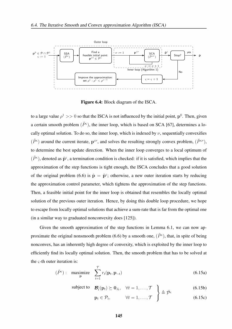
6.4. The Iterative Smooth and Convex approximation Algorithm (ISCA)
SSA(P ς)
p0 ∈ P ∩ P1
ς := 1
Find afeasible initial point:
pς1 ∈ Pςν := 1 SCA
(P ςν)
pςν pς
Stop?yes
p
Improve the approximation:set ρς : ρς < ρς−1 ς:= ς + 1
Outer loop
Inner loop (Algorithm 1)
ν := ν + 1
No
Figure 6.4: Block diagram of the ISCA.
to a large value ρ1 >> 0 so that the ISCA is not influenced by the initial point, p0. Then, given
a certain smooth problem (P ς), the inner loop, which is based on SCA [67], determines a lo-
cally optimal solution. To do so, the inner loop, which is indexed by ν, sequentially convexifies
(P ς) around the current iterate, pςν , and solves the resulting strongly convex problem, (P ςν),
to determine the best update direction. When the inner loop converges to a local optimum of
(P ς), denoted as pς , a termination condition is checked: if it is satisfied, which implies that the
approximation of the step functions is tight enough, the ISCA concludes that a good solution
of the original problem (6.6) is p = pς ; otherwise, a new outer iteration starts by reducing
the approximation control parameter, which tightens the approximation of the step functions.
Then, a feasible initial point for the inner loop is obtained that resembles the locally optimal
solution of the previous outer iteration. Hence, by doing this double loop procedure, we hope
to escape from locally optimal solutions that achieve a sum-rate that is far from the optimal one
(in a similar way to graduated nonconvexity does [125]).
Given the smooth approximation of the step functions in Lemma 6.1, we can now ap-
proximate the original nonsmooth problem (6.6) by a smooth one, (P ς), that, in spite of being
nonconvex, has an inherently high degree of convexity, which is exploited by the inner loop to
efficiently find its locally optimal solution. Then, the smooth problem that has to be solved at
the ς-th outer iteration is:
(P ς) : maximizep
T∑t=1
rt(pt,p−t) (6.15a)
subject to , P ς
Bςt(pt) � 0Jt , ∀t = 1, . . . , T (6.15b)
pt ∈ Pt, ∀t = 1, . . . , T (6.15c)
145
Chapter 6. Sum-rate maximization in multiuser communications with WEHNs considering ageneralized power consumption model
where
[Bςt(pt)]` ,
∑j=1
Etj − Ts∑j=1
∑n∈τtj
K∑k=1
pt(k, n) +Stn∑s=1
wtnsHρς (φtns(pt)), ` = 1, . . . , Jt;
(6.16)
Hρ is given in (6.11); and φtns(pt) is a vector function defined as
φtns(pt) = [φtns1(pt), . . . , φtnsQtns(pt)]T.
Accordingly, we have obtained a smooth nonconvex problem (P ς) in which all the terms
associated with the step functions are either convex or concave. This simplifies the SCA inner
loop, which is presented in the following section.
6.4.1 The inner loop: Nonconvex optimization of smooth problems with
SCA
Among the algorithms that converge to stationary solutions of smooth nonconvex problems
(e.g., gradient-based descend schemes [64], SCA algorithms [65–67], feasible sequential
quadratic programming [68], parallel variable distribution [69], etc.), we have selected the
algorithm in [67] for the inner loop because it has the following main advantages:
• It accepts nonconvex constraints.
• It exploits any degree of convexity present in the problem, which results in a much faster
convergence.
• The problem can be generally solved in a distributed way under very mild assumptions.
• It includes as special cases SCA-based algorithms, such as (proximal) gradient or New-
ton type method, block coordinate (parallel) descent schemes and difference of convex
functions methods.
The algorithm proposed in [67] is based on SCA and consists on solving a sequence of
strongly convex inner approximations of the nonconvex smooth problem. Under some struc-
tural assumptions, the algorithm converges to a locally optimal solution. These assumptions
enforce a specific structure of: (i) the original nonconvex smooth problem [67, Assumption 1];
146

6.4. The Iterative Smooth and Convex approximation Algorithm (ISCA)
(ii) the convex approximation of the objective function [67, Assumption 2]; and (iii) the convex
approximation of the constraints [67, Assumption 3]. In order to use the algorithm in [67] in
our inner loop, we need to satisfy these structural requirements.
It can be easily shown that the smooth problem in (6.15) satisfies (i).
Since the objective function is nonconvex, we need to derive a proper convex approxi-
mation. To do so, we exploit the “partial” concavity of the rate of a certain user, rt(pt,p−t),
w.r.t. its own transmission power pt. Hence, we approximate the objective function in (6.15a)
around the current iterate pςν = (((pςνt (k, n))Kk=1)Nn=1)Tt=1 as
T∑t=1
rt(pt,pςν), where rt(pt,p
ςν) = rt(pt,pςν−t) + πςνTt (pt − pςνt )− bt
2||pt − pςνt ||2.
The term πςνt linearizes the rate functions of the users t′ 6= t w.r.t. pt, i.e.,
πςνt , ((πςνtkn)Kk=1)Nn=1 =∑t′ 6=t
∇ptrt′(pt′ ,p−t′)∣∣∣pςν
with
πςνtkn =∑t′ 6=t
−snrςνt′ (k, n)htt′(k, n)
muiςνt′ (k, n)(1 + snrςνt′ (k, n)); (6.17)
snrςνt (k, n) , htt(k,n)pςνt (k,n)
muiςνt (k,n)and muiςνt (k, n) , σ2
t (k) +∑
t′ 6=t pςνt′ (k, n)ht′t(k, n) are the SINR
and the multiuser interference-plus-noise power experienced by user t given the power profile
pςν . The term bt2||pt − pςνt ||2 with bt ≥ 0 is a proximal regularization term that relaxes the
convergence conditions of the inner loop algorithm or enhances the convergence speed [66].
Finally, we use the convex approximation of the step functions derived in Lemma 6.2 to
approximate the constraints of the smooth problem.
Accordingly, the strongly convex problem that has to be solved in the ν-th inner loop
iteration, which approximates the smooth problem (P ς) around the current iterate, pςν , is
(P ςν) : maximizep
T∑t=1
rt(pt,pςν) (6.18a)
subject to , P ςν
Bςνt (pt; p
ςνt ) � 0Jt , ∀t = 1, . . . , T (6.18b)
pt ∈ Pt, ∀t = 1, . . . , T (6.18c)
147
Chapter 6. Sum-rate maximization in multiuser communications with WEHNs considering ageneralized power consumption model
with [Bςνt (pt; p
ςνt )]` ,
∑j=1
Etj−Ts∑j=1
∑n∈τtj
K∑k=1
pt(k, n)+∑s∈S+tn
wtnsHρς (pt; pςνt ,φtns)+
∑s∈S−tn
wtnsH−ρς (pt; pςνt ,φtns),
(6.19)
where S+tn = {s ∈ [1, Stn] : wtns > 0} and S−tn = {s ∈ [1, Stn] : wtns < 0}; Hρ is given in
Lemma 6.2; and H−ρ is defined as Hρ but swapping the odd and even sets. Note that we have
defined H−ρ because the negative weights invert the concavity or convexity of the terms of the
smooth step function.
Additionally, since the objective function and constraints of the different transmitters are
decoupled, we can apply primal decomposition [126] and solve T parallel problems, one for
each user, which leads to a distributed resource allocation strategy that requires very limited
feedback as presented later. Accordingly, each transmitter must solve the following problem at
each inner loop iteration:
(P ςνt ) : maximize
ptrt(pt,p
ςν) (6.20a)
subject to , P ςνt
Bςνt (pt; p
ςνt ) � 0Jt , (6.20b)
pt ∈ Pt. (6.20c)
Since (P ςνt ) is a strongly convex problem, its unique solution, pςνt , can be easily deter-
mined by classical convex optimization algorithms, e.g., interior point methods [63]. However,
since the solution to (P ςνt ) has to be computed at each inner loop iteration, it is key to derive (if
possible) a closed form solution in order to reduce the computational complexity of the ISCA.
The SCA-based inner loop algorithm that converges to a locally optimal solution of the
smooth nonconvex problem (P ς) is given in Algorithm 6.1 [67]. Basically, the algorithm uses
the unique optimal solution to (P ςνt ), pςνt , to determine the initial point of the following itera-
tion, pς(ν+1)t , which is computed as a convex combination of pςνt and the previous iterate pςνt .
Theorem 6.1 ( [67]). Given the smooth nonconvex problem (P ς), suppose that one of the two
following conditions holds:
a) The step size aςν is such that 0 < infν aςν ≤ supν a
ςν ≤ amax ≤ 1 and 2cr ≥ amaxL∇r,
where cr is the constant of uniform strong convexity of∑T
t=1 rt(pt,pςν) and L∇r is Lipschitz
148
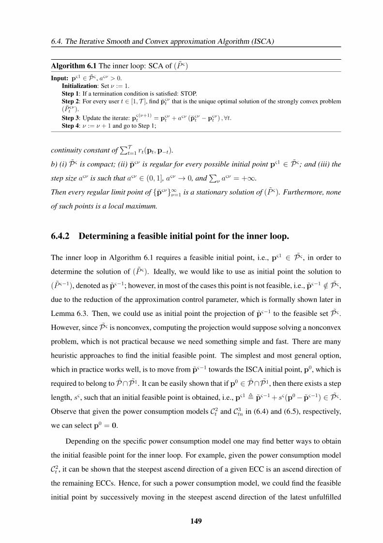
6.4. The Iterative Smooth and Convex approximation Algorithm (ISCA)
Algorithm 6.1 The inner loop: SCA of (P ς)
Input: pς1 ∈ Pς , aςν > 0.Initialization: Set ν := 1.Step 1: If a termination condition is satisfied: STOP.Step 2: For every user t ∈ [1, T ], find pςνt that is the unique optimal solution of the strongly convex problem(P ςνt ).Step 3: Update the iterate: p
ς(ν+1)t = pςνt + aςν (pςνt − pςνt ) ,∀t.
Step 4: ν := ν + 1 and go to Step 1;
continuity constant of∑T
t=1 rt(pt,p−t).
b) (i) P ς is compact; (ii) pςν is regular for every possible initial point pς1 ∈ P ς; and (iii) the
step size aςν is such that aςν ∈ (0, 1], aςν → 0, and∑
ν aςν = +∞.
Then every regular limit point of {pςν}∞ν=1 is a stationary solution of (P ς). Furthermore, none
of such points is a local maximum.
6.4.2 Determining a feasible initial point for the inner loop.
The inner loop in Algorithm 6.1 requires a feasible initial point, i.e., pς1 ∈ P ς , in order to
determine the solution of (P ς). Ideally, we would like to use as initial point the solution to
(P ς−1), denoted as pς−1; however, in most of the cases this point is not feasible, i.e., pς−1 /∈ P ς ,
due to the reduction of the approximation control parameter, which is formally shown later in
Lemma 6.3. Then, we could use as initial point the projection of pς−1 to the feasible set P ς .
However, since P ς is nonconvex, computing the projection would suppose solving a nonconvex
problem, which is not practical because we need something simple and fast. There are many
heuristic approaches to find the initial feasible point. The simplest and most general option,
which in practice works well, is to move from pς−1 towards the ISCA initial point, p0, which is
required to belong to P ∩P1. It can be easily shown that if p0 ∈ P∩P1, then there exists a step
length, sς , such that an initial feasible point is obtained, i.e., pς1 , pς−1 + sς(p0− pς−1) ∈ P ς .
Observe that given the power consumption models C2t and C3
tn in (6.4) and (6.5), respectively,
we can select p0 = 0.
Depending on the specific power consumption model one may find better ways to obtain
the initial feasible point for the inner loop. For example, given the power consumption model
C2t , it can be shown that the steepest ascend direction of a given ECC is an ascend direction of
the remaining ECCs. Hence, for such a power consumption model, we could find the feasible
initial point by successively moving in the steepest ascend direction of the latest unfulfilled
149
Chapter 6. Sum-rate maximization in multiuser communications with WEHNs considering ageneralized power consumption model
ECC, i.e., ∇pt [Bςt(p
ς−1t )]jςt , with jςt = maxj{[Bς
t(pς−1t )]j < 0, j = 1, . . . , Jt}, until the jςt
constraint is satisfied. This process must be repeated until all the constraints are fulfilled.
6.4.3 Convergence of the feasible sets and distributed implementation
Now, the details of all the building blocks of the ISCA have been introduced. The following
lemma characterizes the relations between the feasible sets of the outer loop problems (P ς),
P ς , w.r.t. the feasible set of the original problem, P .3
Lemma 6.3. (a) The sequence of feasible sets of the smooth problems {P ς}∞ς=1 converges to
P , i.e.,
limς→∞P ς → P . (6.21)
(b) If the step function weights are all positive, wtns > 0, ∀t, s, then we have that P ⊆ P∞ ⊂
· · · ⊂ P ς+1 ⊂ P ς ⊂ · · · ⊂ P1.
(c) If the weights are all negative, wtns < 0, ∀t, s, then P1 ⊂ · · · ⊂ P ς ⊂ P ς+1 ⊂ . . . P∞ ⊆ P .
Proof: See Appendix 6.A.2.
Note that when a step function has a positive weight, wtns > 0, it is tightening the ECCs
w.r.t. solely considering the radiated power in the ECCs. Conversely, the ECCs are loosed by
negative weighted step functions. As shown in Table 6.1, the power consumption model C2t
in (6.4) has all the weights positive; whereas, C3tn in (6.5) has positive and negative weights.
Observe that, it would be estrange that a power consumption model had all the weights negative
since it would imply that all the step functions reduce the power consumption.
In the near future we want to use the result on the convergence of the feasible sets in
Lemma 6.3 in order to prove that the sequence of stationary solutions of the smooth problem,
(P ς), obtained by Algorithm 6.1, converges to a stationary solution of the original nonconvex
and nonsmooth problem (P ). We believe that by using the tools of variational analysis [127]
we might be able to obtain the desired proof; however, further research is required.
As argued in §2.1.3, the solution to the offline maximization problem is specially meaning-
ful when the channel and energy harvesting processes can be predicted within the optimization
3Lemma 6.3 uses the limit definition of a sequence of sets, which is given in [127, Definition 4.1]. Basically,the limit exists if the outer and inner limits (see definitions in [127, Definition 4.1]) are equal. In such a case, thelimit is the set given by the inner and outer limits.
150

6.5. The ISCA algorithm for C2t .
time horizon. When this happens, it is key that the power allocation strategy can be com-
puted distributedly by the network nodes because then the nodes can adapt their transmission
strategies when substantial changes on the energy harvesting process are observed.
In order to compute the solution in a distributed manner, the following signaling is required
so that the remaining transmitters can compute the weights πςνtkn: (i) at each outer loop iteration,
each transmitter has to broadcast the feasible initial point of the inner loop; and (ii) at each
inner loop iteration, each transmitter t solely has to broadcast ∇p−trt(pt,pςν−t), which can be
computed with the local measurements of the SINR and the MUI.
Note that the fulfillment of the ECCs is not guaranteed until convergence of the ISCA.
Accordingly, it is required that each of the nodes has a backup battery to be used for this
transitory regime, which can be recharged with the harvested energy.
Remark 6.2. Note that if a different rate function applies, the ISCA can be used by deriving a
proper convex approximation of the objective function.
In the following section, we focus on the power consumption model C2t and derive a closed
form solution of the inner loop problem.
6.5 The ISCA algorithm for C2t .
In this section, we use the ISCA to distributedly compute a locally optimal power allocation
given the power consumption model C2t in (6.4), which is the power consumption model that
we used in Chapter 5.
As it has been mentioned in §6.4, at each inner loop iteration, the t-th transmitter must
solve (6.20) to obtain the update direction. Given the power consumption model C2t , we have
that
[Bςνt (pt; p
ςνt )]` =
∑j=1
Etj −∑n∈τj
(εςνt (n) +
K∑k=1
ϕςνt (k, n)pt(k, n)
) , with (6.22)
ϕςνt (k, n) = Ts
(1 +
αtρςe−
∑Kk=1 p
ςνt (k,n)
ρς +βtρςe−pςνt (k,n)
ρς
)and (6.23)
151
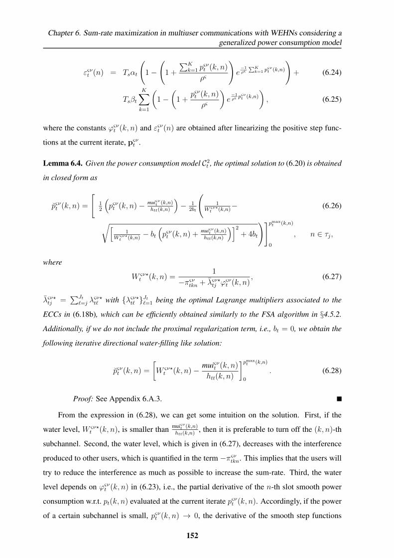
Chapter 6. Sum-rate maximization in multiuser communications with WEHNs considering ageneralized power consumption model
εςνt (n) = Tsαt
(1−
(1 +
∑Kk=1 p
ςνt (k, n)
ρς
)e−1ρς
∑Kk=1 p
ςνt (k,n)
)+ (6.24)
Tsβt
K∑k=1
(1−
(1 +
pςνt (k, n)
ρς
)e−1ρςpςνt (k,n)
), (6.25)
where the constants ϕςνt (k, n) and εςνt (n) are obtained after linearizing the positive step func-
tions at the current iterate, pςνt .
Lemma 6.4. Given the power consumption model C2t , the optimal solution to (6.20) is obtained
in closed form as
pςνt (k, n) =
[12
(pςνt (k, n)− muiςνt (k,n)
htt(k,n)
)− 1
2bt
(1
W ςν?t (k,n)
− (6.26)
√[1
W ςν?t (k,n)
− bt(pςνt (k, n) +
muiςνt (k,n)
htt(k,n)
)]2
+ 4bt
)]pmaxt (k,n)
0
, n ∈ τj,
where
W ςν?t (k, n) =
1
−πςνtkn + λςν?tj ϕςνt (k, n)
, (6.27)
λςν?tj =∑Jt
`=j λςν?t` with {λςν?t` }
Jt`=1 being the optimal Lagrange multipliers associated to the
ECCs in (6.18b), which can be efficiently obtained similarly to the FSA algorithm in §4.5.2.
Additionally, if we do not include the proximal regularization term, i.e., bt = 0, we obtain the
following iterative directional water-filling like solution:
pςνt (k, n) =
[W ςν?t (k, n)− muiςνt (k, n)
htt(k, n)
]pmaxt (k,n)
0
. (6.28)
Proof: See Appendix 6.A.3.
From the expression in (6.28), we can get some intuition on the solution. First, if the
water level, W ςν?t (k, n), is smaller than muiςνt (k,n)
htt(k,n), then it is preferable to turn off the (k, n)-th
subchannel. Second, the water level, which is given in (6.27), decreases with the interference
produced to other users, which is quantified in the term −πςνtkn. This implies that the users will
try to reduce the interference as much as possible to increase the sum-rate. Third, the water
level depends on ϕςνt (k, n) in (6.23), i.e., the partial derivative of the n-th slot smooth power
consumption w.r.t. pt(k, n) evaluated at the current iterate pςνt (k, n). Accordingly, if the power
of a certain subchannel is small, pςνt (k, n) → 0, the derivative of the smooth step functions
152
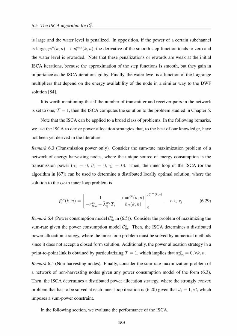
6.5. The ISCA algorithm for C2t .
is large and the water level is penalized. In opposition, if the power of a certain subchannel
is large, pςνt (k, n) → pmaxt (k, n), the derivative of the smooth step function tends to zero and
the water level is rewarded. Note that these penalizations or rewards are weak at the initial
ISCA iterations, because the approximation of the step functions is smooth, but they gain in
importance as the ISCA iterations go by. Finally, the water level is a function of the Lagrange
multipliers that depend on the energy availability of the node in a similar way to the DWF
solution [84].
It is worth mentioning that if the number of transmitter and receiver pairs in the network
is set to one, T = 1, then the ISCA computes the solution to the problem studied in Chapter 5.
Note that the ISCA can be applied to a broad class of problems. In the following remarks,
we use the ISCA to derive power allocation strategies that, to the best of our knowledge, have
not been yet derived in the literature.
Remark 6.3 (Transmission power only). Consider the sum-rate maximization problem of a
network of energy harvesting nodes, where the unique source of energy consumption is the
transmission power (αt = 0, βt = 0, γt = 0). Then, the inner loop of the ISCA (or the
algorithm in [67]) can be used to determine a distributed locally optimal solution, where the
solution to the ςν-th inner loop problem is
pςνt (k, n) =
[1
−πςνtkn + λςν?tj Ts− muiςνt (k, n)
htt(k, n)
]pmaxt (k,n)
0
, n ∈ τj. (6.29)
Remark 6.4 (Power consumption model C3tn in (6.5)). Consider the problem of maximizing the
sum-rate given the power consumption model C3tn. Then, the ISCA determines a distributed
power allocation strategy, where the inner loop problem must be solved by numerical methods
since it does not accept a closed form solution. Additionally, the power allocation strategy in a
point-to-point link is obtained by particularizing T = 1, which implies that πςνtkn = 0,∀k, n.
Remark 6.5 (Non-harvesting nodes). Finally, consider the sum-rate maximization problem of
a network of non-harvesting nodes given any power consumption model of the form (6.3).
Then, the ISCA determines a distributed power allocation strategy, where the strongly convex
problem that has to be solved at each inner loop iteration is (6.20) given that Jt = 1, ∀t, which
imposes a sum-power constraint.
In the following section, we evaluate the performance of the ISCA.
153
Chapter 6. Sum-rate maximization in multiuser communications with WEHNs considering ageneralized power consumption model
6.6 Results
In this section, we numerically evaluate the performance of the ISCA in terms of achieved rate
and computational complexity of the algorithm.
As it has been argued in the state of the art in Chapter 2, there are few works that consider
the different energy sinks at each transmitter; indeed, to the best of our knowledge, the most
similar work to the problem studied in this chapter is the problem that we studied in Chapter
5, where we considered the mutual information maximization problem in a point-to-point link
with the power consumption model C2t .
Accordingly, in order to have some benchmark with which to compare the performance
of the ISCA, we particularize the solution derived in the previous section to a point-to-point
link by setting T = 1. The remaining system parameters have been set as follows. We have
considered N = 50 channel accesses of duration Ts = 20 ms in which symbols are transmitted
through K = 2 parallel streams. The power consumption constants are set to αt = γt =
150 mW and βt = 10 mW. A Rayleigh fading channel has been considered with unit mean
channel power gain. The energy harvesting process is modeled as a compound Poisson process
as done in [84], where the arrival instants follow a Poisson distribution with rate 110
and the
energy in the packets is drawn from a uniform distribution and normalized by the total harvested
energy that varies along the x-axis of Figures 6.5-6.7. The initial point of the ISCA is set to
zero, and the approximation control parameter is ρς = 0.5ρς−1 with ρ1 = 5. We have not
used the proximal regularization term, bt = 0, and the step size of the inner loop is aςν =
aς(ν−1)(1− 10−3aς(ν−1)) with aς0 = 1, ∀ς .
We consider two classes of strategies:
• Power consumption model C2t : On the one hand, we consider strategies that use the
power consumption model C2t (i.e., strategies that disregard the startup power consump-
tion, γt = 0), which can be based either on the use of IVs or on the use of the ISCA: (i)
the IVs based strategies are the upper bound and feasible solution obtained through inte-
ger relaxation as it has been explained in §5.3.1, which we label here as IV-UB (γt = 0)
and IV (γt = 0); (ii) the ISCA based strategies are ISCA-FSA (γt = 0) that uses the
closed form solution derived in Lemma 6.4, where the Lagrange multipliers are obtained
similarly to the FSA algorithm (cf. §4.5.2), and ISCA-BM (γt = 0) that solves (6.20)
154
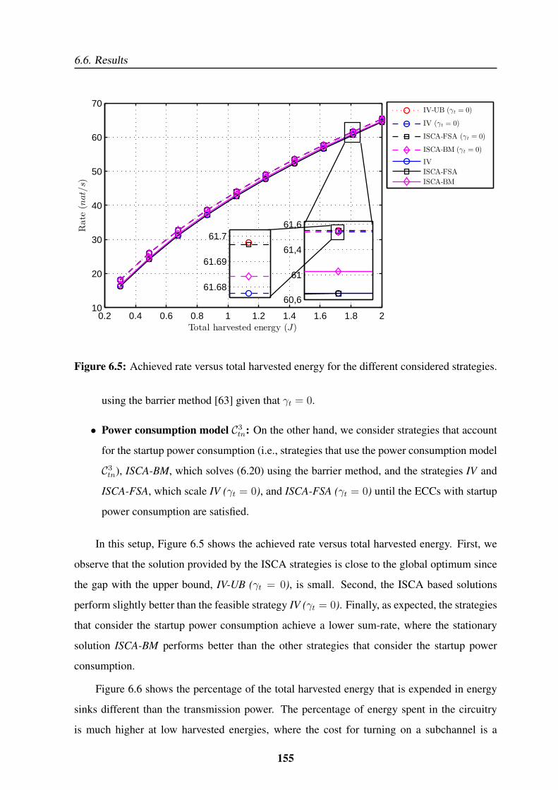
6.6. Results
0.2 0.4 0.6 0.8 1 1.2 1.4 1.6 1.8 210
20
30
40
50
60
70
Total harvested energy (J)
Rate
(nat/s)
60,6
61
61,4
61,6
61.68
61.69
61.7
IV-UB (γt = 0)
IV (γt = 0)
ISCA-FSA (γt = 0)
ISCA-BM (γt = 0)
IV
ISCA-FSA
ISCA-BM
Figure 6.5: Achieved rate versus total harvested energy for the different considered strategies.
using the barrier method [63] given that γt = 0.
• Power consumption model C3tn: On the other hand, we consider strategies that account
for the startup power consumption (i.e., strategies that use the power consumption model
C3tn), ISCA-BM, which solves (6.20) using the barrier method, and the strategies IV and
ISCA-FSA, which scale IV (γt = 0), and ISCA-FSA (γt = 0) until the ECCs with startup
power consumption are satisfied.
In this setup, Figure 6.5 shows the achieved rate versus total harvested energy. First, we
observe that the solution provided by the ISCA strategies is close to the global optimum since
the gap with the upper bound, IV-UB (γt = 0), is small. Second, the ISCA based solutions
perform slightly better than the feasible strategy IV (γt = 0). Finally, as expected, the strategies
that consider the startup power consumption achieve a lower sum-rate, where the stationary
solution ISCA-BM performs better than the other strategies that consider the startup power
consumption.
Figure 6.6 shows the percentage of the total harvested energy that is expended in energy
sinks different than the transmission power. The percentage of energy spent in the circuitry
is much higher at low harvested energies, where the cost for turning on a subchannel is a
155
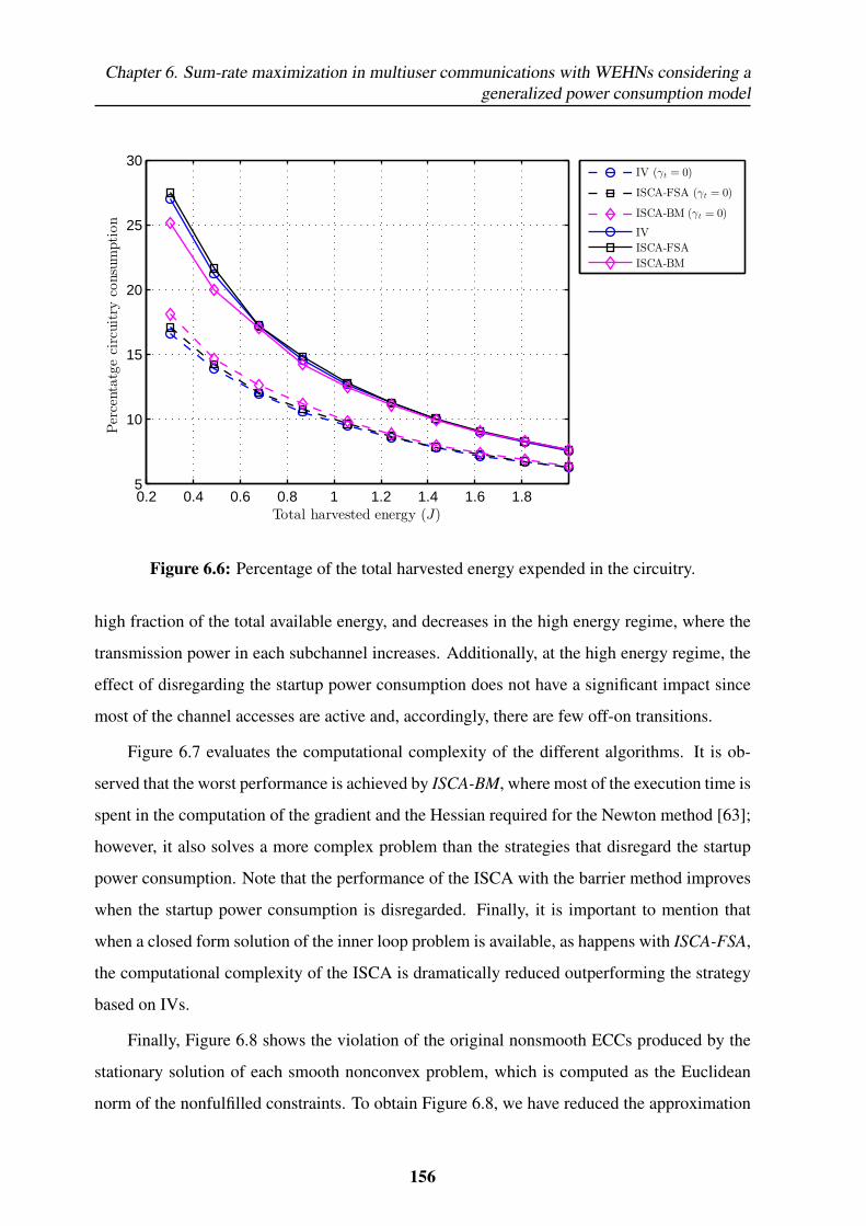
Chapter 6. Sum-rate maximization in multiuser communications with WEHNs considering ageneralized power consumption model
0.2 0.4 0.6 0.8 1 1.2 1.4 1.6 1.85
10
15
20
25
30
Percentatgecircuitry
consumption
Total harvested energy (J)
IV (γt = 0)
ISCA-FSA (γt = 0)
ISCA-BM (γt = 0)
IV
ISCA-FSA
ISCA-BM
Figure 6.6: Percentage of the total harvested energy expended in the circuitry.
high fraction of the total available energy, and decreases in the high energy regime, where the
transmission power in each subchannel increases. Additionally, at the high energy regime, the
effect of disregarding the startup power consumption does not have a significant impact since
most of the channel accesses are active and, accordingly, there are few off-on transitions.
Figure 6.7 evaluates the computational complexity of the different algorithms. It is ob-
served that the worst performance is achieved by ISCA-BM, where most of the execution time is
spent in the computation of the gradient and the Hessian required for the Newton method [63];
however, it also solves a more complex problem than the strategies that disregard the startup
power consumption. Note that the performance of the ISCA with the barrier method improves
when the startup power consumption is disregarded. Finally, it is important to mention that
when a closed form solution of the inner loop problem is available, as happens with ISCA-FSA,
the computational complexity of the ISCA is dramatically reduced outperforming the strategy
based on IVs.
Finally, Figure 6.8 shows the violation of the original nonsmooth ECCs produced by the
stationary solution of each smooth nonconvex problem, which is computed as the Euclidean
norm of the nonfulfilled constraints. To obtain Figure 6.8, we have reduced the approximation
156
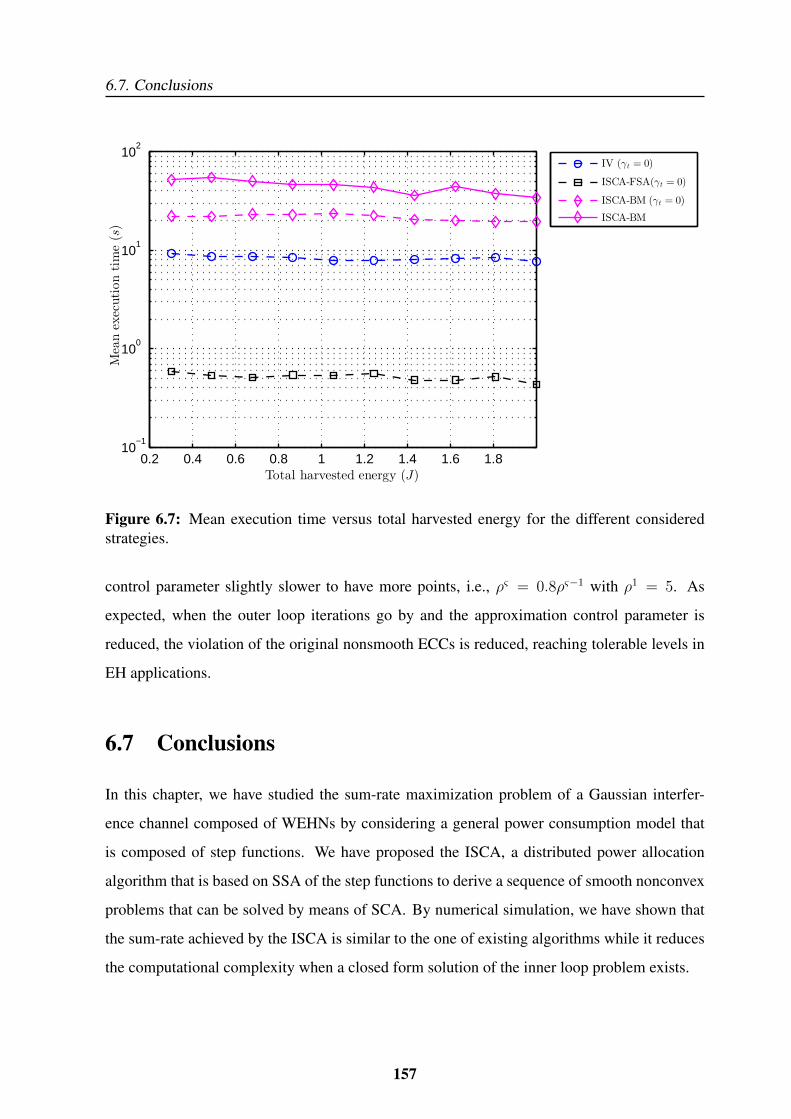
6.7. Conclusions
0.2 0.4 0.6 0.8 1 1.2 1.4 1.6 1.810
−1
100
101
102
Total harvested energy (J)
Meanexecutiontime(s)
IV (γt = 0)
ISCA-FSA(γt = 0)
ISCA-BM (γt = 0)
ISCA-BM
Figure 6.7: Mean execution time versus total harvested energy for the different consideredstrategies.
control parameter slightly slower to have more points, i.e., ρς = 0.8ρς−1 with ρ1 = 5. As
expected, when the outer loop iterations go by and the approximation control parameter is
reduced, the violation of the original nonsmooth ECCs is reduced, reaching tolerable levels in
EH applications.
6.7 Conclusions
In this chapter, we have studied the sum-rate maximization problem of a Gaussian interfer-
ence channel composed of WEHNs by considering a general power consumption model that
is composed of step functions. We have proposed the ISCA, a distributed power allocation
algorithm that is based on SSA of the step functions to derive a sequence of smooth nonconvex
problems that can be solved by means of SCA. By numerical simulation, we have shown that
the sum-rate achieved by the ISCA is similar to the one of existing algorithms while it reduces
the computational complexity when a closed form solution of the inner loop problem exists.
157
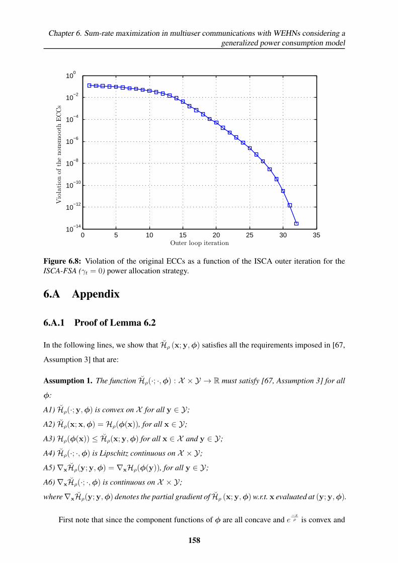
Chapter 6. Sum-rate maximization in multiuser communications with WEHNs considering ageneralized power consumption model
0 5 10 15 20 25 30 3510
−14
10−12
10−10
10−8
10−6
10−4
10−2
100
Outer loop iteration
Violationofthenonsm
ooth
ECCs
Figure 6.8: Violation of the original ECCs as a function of the ISCA outer iteration for theISCA-FSA (γt = 0) power allocation strategy.
6.A Appendix
6.A.1 Proof of Lemma 6.2
In the following lines, we show that Hρ (x; y,φ) satisfies all the requirements imposed in [67,
Assumption 3] that are:
Assumption 1. The function Hρ(·; ·,φ) : X × Y → R must satisfy [67, Assumption 3] for all
φ:
A1) Hρ(·; y,φ) is convex on X for all y ∈ Y;
A2) Hρ(x; x,φ) = Hρ(φ(x)), for all x ∈ Y;
A3)Hρ(φ(x)) ≤ Hρ(x; y,φ) for all x ∈ X and y ∈ Y;
A4) Hρ(·; ·,φ) is Lipschitz continuous on X × Y;
A5) ∇xHρ(y; y,φ) = ∇xHρ(φ(y)), for all y ∈ Y;
A6) ∇xHρ(·; ·,φ) is continuous on X × Y;
where∇xHρ(y; y,φ) denotes the partial gradient of Hρ (x; y,φ) w.r.t. x evaluated at (y; y,φ).
First note that since the component functions of φ are all concave and e−xρ is convex and
158
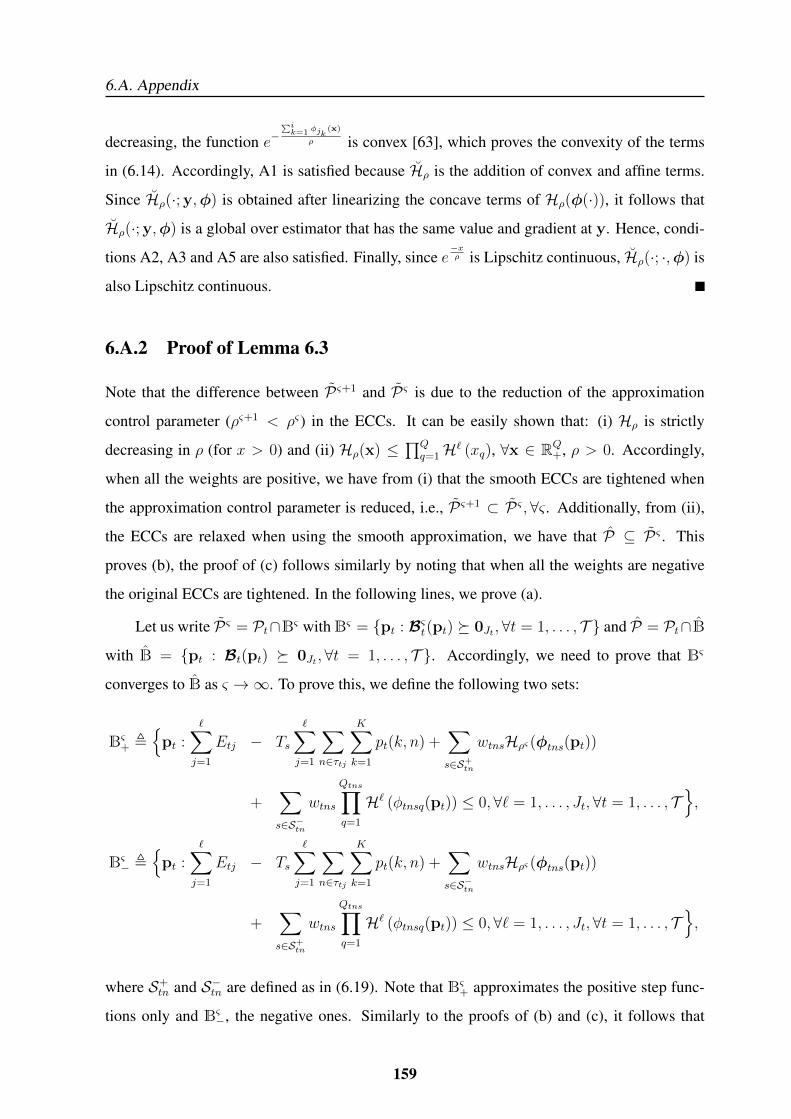
6.A. Appendix
decreasing, the function e−∑ik=1 φjk
(x)
ρ is convex [63], which proves the convexity of the terms
in (6.14). Accordingly, A1 is satisfied because Hρ is the addition of convex and affine terms.
Since Hρ(·; y,φ) is obtained after linearizing the concave terms of Hρ(φ(·)), it follows that
Hρ(·; y,φ) is a global over estimator that has the same value and gradient at y. Hence, condi-
tions A2, A3 and A5 are also satisfied. Finally, since e−xρ is Lipschitz continuous, Hρ(·; ·,φ) is
also Lipschitz continuous.
6.A.2 Proof of Lemma 6.3
Note that the difference between P ς+1 and P ς is due to the reduction of the approximation
control parameter (ρς+1 < ρς) in the ECCs. It can be easily shown that: (i) Hρ is strictly
decreasing in ρ (for x > 0) and (ii) Hρ(x) ≤∏Q
q=1H` (xq), ∀x ∈ RQ+, ρ > 0. Accordingly,
when all the weights are positive, we have from (i) that the smooth ECCs are tightened when
the approximation control parameter is reduced, i.e., P ς+1 ⊂ P ς ,∀ς . Additionally, from (ii),
the ECCs are relaxed when using the smooth approximation, we have that P ⊆ P ς . This
proves (b), the proof of (c) follows similarly by noting that when all the weights are negative
the original ECCs are tightened. In the following lines, we prove (a).
Let us write P ς = Pt∩Bς withBς = {pt : Bςt(pt) � 0Jt ,∀t = 1, . . . , T } and P = Pt∩B
with B = {pt : Bt(pt) � 0Jt ,∀t = 1, . . . , T }. Accordingly, we need to prove that Bς
converges to B as ς →∞. To prove this, we define the following two sets:
Bς+ ,{
pt :∑j=1
Etj − Ts∑j=1
∑n∈τtj
K∑k=1
pt(k, n) +∑s∈S+tn
wtnsHρς (φtns(pt))
+∑s∈S−tn
wtns
Qtns∏q=1
H` (φtnsq(pt)) ≤ 0,∀` = 1, . . . , Jt,∀t = 1, . . . , T},
Bς− ,{
pt :∑j=1
Etj − Ts∑j=1
∑n∈τtj
K∑k=1
pt(k, n) +∑s∈S−tn
wtnsHρς (φtns(pt))
+∑s∈S+tn
wtns
Qtns∏q=1
H` (φtnsq(pt)) ≤ 0,∀` = 1, . . . , Jt,∀t = 1, . . . , T},
where S+tn and S−tn are defined as in (6.19). Note that Bς+ approximates the positive step func-
tions only and Bς−, the negative ones. Similarly to the proofs of (b) and (c), it follows that
159
Chapter 6. Sum-rate maximization in multiuser communications with WEHNs considering ageneralized power consumption model
Bς+1+ ⊂ Bς+,∀ς and Bς− ⊂ Bς+1
− ,∀ς . Additionally, following the same arguments, we have that
Bς− ⊂ Bς ⊂ Bς+. From [127, Exercise 4.3], we have that the limits of the setsBς+ andBς− exists
(the inner and outer limits are equal) and are Bς+ → B and Bς− → B. This leads to Bς → B,
which proves (a).
6.A.3 Proof of Lemma 6.4
We prove Lemma 3 by using the KKT sufficient optimality conditions. The Lagrangian of
the problem in (6.20) is Lςνt (pt,λςνt ) = rt(pt,p
ςν−t) + πςνTt (pt − pςνt ) − bt
2||pt − pςνt ||2 +
λςνTt Bςνt (pt; p
ςνt ), where λςνt are the Lagrange multipliers associated to the ECCs in (6.20b).
Taking the derivative of the Lagrangian w.r.t. pt(k, n), n ∈ τj , and equating to zero, we have
pςνt (k, n) =
0 if 1W ςνt (k,n)
≥ htt(k,n)muiςνt (k,n)
+ btpςνt (k, n),
pςνt (k, n) if 1W ςνt (k,n)
< htt(k,n)muiςνt (k,n)
+ btpςνt (k, n), and
1W ςνt (k,n)
> htt(k,n)htt(k,n)pmax
t (k,n)+muiςνt (k,n)− bt(pmax
t (k, n)− pςνt (k, n)),
pmaxt (k, n) if 1
W ςνt (k,n)
≤ htt(k,n)htt(k,n)pmax
t (k,n)+muiςνt (k,n)− bt(pmax
t (k, n)− pςνt (k, n)),
where W ςνt (k, n) = 1
−πςνtkn+λςνtj ϕςνt (k,n)
with λςνtj =∑J
`=j λςνt` ; and pςνt (k, n) is obtained as the
solution of the following quadratic equation
htt(k, n)
htt(k, n)pςνt (k, n) + muiςνt (k, n)=
1
W ςνt (k, n)
+ bt(pςνt (k, n)− pςνt (k, n)). (6.30)
From [128, Lemma 35] (with Hk := htt(k,n)muiςνt (k,n)
, τ := bt, ck := pςνt (k, n), µk := 1W ςνt (k,n)
),
the previous equation has the following properties: (i) both roots are real, one root is always
negative, and the other is nonnegative; (ii) both roots are increasing in W ςνt (k, n); and from the
expression of the nonnegative root, we obtain (6.26).
Finally, note that if the proximal step is zero, i.e., bt = 0, then (6.28) follows directly from
the first order equation in (6.30).
160
Chapter 7Thesis conclusions and future work
7.1 Conclusions
This dissertation has focused on the design of transmission strategies (linear precoding designs
and resource allocation strategies) that take into account the specific characteristics of WEHNs.
In particular, the dissertation has put an special emphasis on taking into account the energy
availability variations and the different sources of energy consumption at the transmitter(s),
which are not accounted for in classical transmission strategies. As a result, the proposed
transmission strategies exploit more efficiently the available energy than classical transmission
strategies improving the achieved performance given some figure of merit.
In Chapter 1, we have motivated the conducted research and presented the outline and
research contributions of the dissertation.
Chapter 2 has presented the structure of a WEHN and the main characteristics that must
be taken into account when designing transmission strategies for WEHNs. Additionally, the
chapter has overviewed the state of the art on well-known transmission strategies.
Chapter 3 has considered an energy harvesting transmitter operating in a point-to-point
link with a time-static channel that has a finite battery capacity, acquires the data packets over
time, and has to fulfill some QoS constraint. This chapter has studied the (offline) data depar-
ture curve that minimizes the transmission completion time by satisfying the DCC, the ECC,
and the QoS constraint. The optimal transmission strategy has been constructed by deriving
structural properties of the solution: first, it has been shown that constant rate transmission is
the strategy that requires less energy to transmit a certain amount of data if no energy is lost due
161

Chapter 7. Thesis conclusions and future work
to battery overflows; afterwards, it has been shown that losing energy due to battery overflows
is suboptimal as far as there is data to be transmitted and, accordingly, it is better to increase
the rate before the overflow until either there is no overflow or the DCC is reached (i.e., there
is no more data to transmit); finally, it has been demonstrated that the existence of the optimal
solution depends both on the dynamics of the harvesting process and on the required QoS. Ac-
cording to these properties, an algorithm has been proposed that is able to determine whether
the problem has a solution or not and, in case of having a solution, determines the optimal data
departure curve.
Chapter 4 has been devoted to a WEHN transmitting arbitrarily distributed symbols in a
discrete-time linear vector Gaussian channel. The chapter has investigated the offline linear
precoding strategy that maximizes the mutual information by taking into account the causality
constraints on the use of energy when there is an infinite backlog of data waiting to be trans-
mitted. The chapter has proved that the optimal left singular vectors of the precoder matrix
diagonalize the channel and argued that the derivation of the optimal right singular vectors is
an involved problem that is left for future research. Then, the chapter has focused in the prac-
tical situation in which the right singular vectors are set to the identity matrix; in this setup,
the optimal offline power allocation, the MIMO Mercury Water-Flowing solution, has been
derived. The chapter has presented two different algorithms that compute the offline MIMO
Mercury Water-Flowing solution whose computational complexity has been evaluated both an-
alytically and experimentally; additionally, an online algorithm has been proposed. Finally,
the performance of the different algorithms has been compared through numerical simulations
showing a substantial increase in the achieved mutual information.
Chapter 5 has studied the power allocation strategy that maximizes the mutual informa-
tion achieved by a WEHN along N independent channel accesses in which symbols are sent
through K parallel streams. The main contribution of Chapter 5 w.r.t. previous works like
DWF is that, not only the transmission radiated power has been accounted for in the ECCs,
but also the cost associated with having a certain channel access or stream “on”. The offline
maximization problem has been shown to be nonsmooth and nonconvex due to the presence
of step functions on the power consumption model. After replacing the step functions by ad-
ditional optimization variables, named IVs, the chapter has explored the integer relaxation and
dual problems to obtain two suboptimal solutions and an upper bound of the original offline
maximization problem. Interestingly, we have shown that these feasible solutions are practi-
162
7.2. Future Work
cally identical in the sense that a common condition for the activation of the channel access
and streams is obtained, i.e., if the epoch water level is greater than the corresponding cutoff
water level, and asymptotically tend to the optimal solution when the number of channel ac-
cesses or streams per epoch is large. Additionally, we have devised the Boxed Water-Flowing,
an intuitive graphical representation of the asymptotically optimal offline resource allocation,
which is based on the cutoff water level concept. Finally, a practical online algorithm has been
proposed, which requires the lowest execution time compared to the offline algorithms and has
a small performance loss.
Finally, Chapter 6 has focused on a multiuser communication system and has investigated
the power allocation strategy in each transmitter that maximizes the network’s sum-rate when a
generalized power consumption model is considered in the ECCs, which is composed of prod-
ucts and summations of step functions. To address the problem, the ISCA has been proposed
that is based on SSA of the indicator functions to derive a sequence of smooth nonconvex prob-
lems that can be solved by means of SCA. As it has been presented, one of the key features of
the proposed algorithm is that the power allocation strategy can be computed in a distributed
manner by the network nodes. By numerical simulation, we have shown that, under the setup
of Chapter 5 (a point-to-point communication with channel access and stream activation costs),
the mutual information achieved by the ISCA is similar to the asymptotically optimal Boxed
Water-Flowing solution while it reduces the computational complexity.
7.2 Future Work
There are a myriad of possible research directions that can be considered to extend the results
obtained in this work. In short, for the design of more efficient transmission strategies, it is key
to develop better models of both the energy generation and consumption processes.
First of all, given the current available models of the energy generation and consumption
processes, there are still many offline transmission strategies that should be investigated:
• This thesis has only considered the transmission completion time minimization and the
mutual information maximization; accordingly, one possible research direction is the
consideration of different figures of merit (for example, the ones discussed in §2.1.5).
• Regarding practical communication systems that use an arbitrary input distribution, the
163

Chapter 7. Thesis conclusions and future work
following research lines can be considered:
– To determine the optimal right singular vectors of the precoding matrix under the
setup studied in Chapter 4.
– To determine the optimal linear precoder with the generalized power consumption
model C4 introduced in Chapter 6.
– To allow a dynamic selection of the modulation and coding schemes according to
the node energy availability.
As briefly discussed in §2.1.1, few works have dealt with the modeling of the energy har-
vesting process given the different energy sources and transducers. Accordingly, the following
research directions are required in the upcoming years:
• To develop measurement campaigns of the harvested energy given different energy sour-
ces and harvesting technologies (in a similar way than the measurements of the solar and
kinetic energies obtained in [31, 35, 36]). These measurement campaigns must be broad
enough to capture the energy variability due to environmental and climatic conditions as
well as node’s placement and mobility.
• To create statistical models of the acquired data in the previous point in order to design:
– Low-complexity prediction algorithms of the harvested energy that can be used
prior to the computation of the offline transmission strategy.
– Online algorithms that exploit the available statistical knowledge of the harvested
energy.
Additionally, for the design of accurate offline and online transmission strategies it is key
to analyze the impact of not having complete CSI at the transmitter.
This work has proposed a generalized power consumption model, but still many sources
of power consumption escape from the model and should be considered:
• Energy consumption at the processing unit to perform the computation of the transmis-
sion strategy:
As we have seen throughout this dissertation, the computation of the transmission strat-
egy entails a certain computational complexity, which in general grows with the num-
ber of channel accesses, N , (or optimization time horizon), the number of parallel data
164

7.2. Future Work
streams, K, and the number of energy packets or ECCs, J . This computational com-
plexity has an associated energy consumption which has been ignored in the designed
transmission strategies (and, to the best of our knowledge, in all the related works in the
literature).
On the one hand, when this source of energy consumption is neglected, a larger optimiza-
tion time horizon is always preferred in terms of achievable performance; additionally,
as it has been argued in §2.1.1, the packetized model of the energy harvesting process
can be understood as a time sampling of the continuous power harvesting profile, where
the smaller the sampling window (or the greater the value of J), the more the packe-
tized model resembles to the real power harvesting profile, which also results in a better
performance.
On the other hand, if this source of energy consumption is considered, there exists a
tradeoff in the selection of the parameters N and J , which should be carefully analyzed
and studied, since larger values of N and J imply a loss on the total available energy for
transmission due to the higher energy consumption to compute the transmission strategy.
• Energy consumption of the sensors to acquire data:
A wireless sensor node consumes a substantial amount of energy for sensing purposes
(in the sensor itself and to perform the analog to digital conversion of the sensed data),
which has been generally ignored when designing the node’s transmission strategy. This
source of consumption opens a new research paradigm since the sensing and transmission
policies must be jointly designed to achieve the best performance given some figure of
merit.
165

BIBLIOGRAPHY
Bibliography
[1] European Comission, “Addressing the challenge of energy efficiency through informa-
tion and communication technologies,” May 2008.
[2] G. E. Moore, “Cramming more components onto integrated circuits,” IEEE Solid-State
Circuits Society Newsletter, vol. 11, no. 5, pp. 33–35, Sep. 2006.
[3] W. Vereecken, W. V. Heddeghem, D. Colle, M. Pickavet, and P. Demeester, “Overall
ICT footprint and green communication technologies,” in proceedings of the 4th Inter-
national Symposium on Communications, Control and Signal Processing, Mar. 2010,
pp. 1–6.
[4] J. A. Paradiso and T. Starner, “Energy scavenging for mobile and wireless electronics,”
IEEE Pervasive Comput., vol. 4, no. 1, pp. 18 – 27, Jan. 2005.
[5] Yole Developpement, “Emerging energy harvesting devices,” Nov. 2012.
[6] M. Gregori and M. Payaro, “Efficient data transmission for an energy harvesting node
with battery capacity constraint,” in Proceedings of the IEEE Global Telecommunica-
tions Conference, Dec. 2011, pp. 1–6.
[7] ——, “Energy-efficient transmission for wireless energy harvesting nodes,” IEEE Trans.
on Wireless Communications, vol. 12, no. 3, pp. 1244–1254, Mar. 2013.
[8] ——, “Optimal power allocation for a wireless multi-antenna energy harvesting node
with arbitrary input distribution,” in Proceedings of the IEEE International Conference
on Communications, Jun. 2012, pp. 5794 –5798.
167
BIBLIOGRAPHY
[9] ——, “On the precoder design of a wireless energy harvesting node in linear vector
Gaussian channels with arbitrary input distribution,” IEEE Trans. on Communications,
vol. 61, no. 5, pp. 1868–1879, May 2013.
[10] ——, “Throughput maximization for a wireless energy harvesting node considering the
circuitry power consumption,” in Proceedings of the IEEE Vehicular Technology Con-
ference, Sep. 2012, pp. 1–5.
[11] M. Gregori, A. Pascual-Iserte, and M. Payaro, “Mutual information maximization for a
wireless energy harvesting node considering the circuitry power consumption,” in Pro-
ceedings of the IEEE Wireless Communications and Networking Conference, Apr. 2013,
pp. 4238–4243.
[12] M. Gregori and M. Payaro, “On the optimal resource allocation for a wireless energy
harvesting node considering the circuitry power consumption,” accepted in IEEE Trans.
on Wireless Communications, Jun. 2014.
[13] ——, “Multiuser communications with energy harvesting transmitters,” in Proceedings
of the IEEE International Conference on Communications, 2014.
[14] M. Payaro, M. Gregori, and D. P. Palomar, “Yet another entropy power inequality with
an application,” in Proceedings of the IEEE International Conference on Wireless Com-
munications and Signal Processing, Nov. 2011, pp. 1–5.
[15] A. Kansal, J. Hsu, S. Zahedi, and M. B. Srivastava, “Power management in energy har-
vesting sensor networks,” ACM Transactions on Embedded Computing Systems, vol. 6,
no. 4, p. 32, Sep. 2007.
[16] S. Sudevalayam and P. Kulkarni, “Energy harvesting sensor nodes: Survey and implica-
tions,” IEEE Commun. Surveys Tuts., vol. 13, no. 3, pp. 443–461, Third Quarter 2011.
[17] N. Wang, N. Zhang, and M. Wang, “Wireless sensors in agriculture and food indus-
try—recent development and future perspective,” Computers and electronics in agricul-
ture, vol. 50, no. 1, pp. 1–14, Jan. 2006.
[18] I. F. Akyildiz, T. Melodia, and K. R. Chowdhury, “A survey on wireless multimedia
sensor networks,” Computer networks, vol. 51, no. 4, pp. 921–960, Mar. 2007.
168
BIBLIOGRAPHY
[19] D. Gunduz, K. Stamatiou, N. Michelusi, and M. Zorzi, “Designing intelligent energy
harvesting communication systems,” IEEE Commun. Mag., vol. 52, no. 1, pp. 210–216,
Jan. 2014.
[20] D. P. Palomar, “A unified framework for communications through MIMO channels,”
Ph.D. dissertation, Technical University of Catalonia (UPC), Barcelona, Spain, 2003.
[21] M. Payaro, “Impact of channel state information on the analysis and design of multi-
antenna communication systems,” Ph.D. dissertation, Technical University of Catalonia
(UPC), Barcelona, Spain, 2006.
[22] R. J. Vullers, R. Schaijk, H. J. Visser, J. Penders, and C. V. Hoof, “Energy harvesting for
autonomous wireless sensor networks,” IEEE J. Solid-State Circuits, vol. 2, no. 2, pp.
29–38, Spring 2010.
[23] “Cebekit: Windlab junior c-0200 technical characteristics.” [Online]. Available:
http://fadisel.cat/docs/c-0200-ing.pdf
[24] H. J. Visser, A. C. Reniers, and J. A. Theeuwes, “Ambient RF energy scavenging: GSM
and WLAN power density measurements,” in Proceedings of the IEEE European Mi-
crowave Conference, Oct. 2008, pp. 721–724.
[25] W. K. Seah, Z. A. Eu, and H.-P. Tan, “Wireless sensor networks powered by ambient en-
ergy harvesting (wsn-heap)-survey and challenges,” in Proceedings of the IEEE Wireless
Communication, Vehicular Technology, Information Theory and Aerospace & Electronic
Systems Technology, May 2009, pp. 1–5.
[26] L. Mateu, C. Codrea, N. Lucas, M. Pollak, and P. Spies, “Energy harvesting for wireless
communication systems using thermogenerators,” in Proceeding of the XXI Conference
on Design of Circuits and Integrated Systems, Nov. 2006.
[27] C. Park and P. H. Chou, “Ambimax: Autonomous energy harvesting platform for multi-
supply wireless sensor nodes,” in Proceedings of the IEEE Sensor and Ad Hoc Commu-
nications and Networks, vol. 1, Sep. 2006, pp. 168–177.
169
BIBLIOGRAPHY
[28] Y. K. Tan and S. K. Panda, “Self-autonomous wireless sensor nodes with wind energy
harvesting for remote sensing of wind-driven wildfire spread,” IEEE Trans. Instrum.
Meas., vol. 60, no. 4, pp. 1367–1377, Apr. 2011.
[29] S. J. Roundy, “Energy scavenging for wireless sensor nodes with a focus on vibration to
electricity conversion,” Ph.D. dissertation, University of California, 2003.
[30] S. P. Beeby, M. J. Tudor, and N. M. White, “Energy harvesting vibration sources for
microsystems applications,” Measurement Science and Technology, vol. 17, no. 12, p.
R175, 2006.
[31] M. Gorlatova, J. Sarik, M. Cong, I. Kymissis, and G. Zussman, “Movers and shakers:
Kinetic energy harvesting for the internet of things,” arXiv preprint:1307.0044, 2013.
[32] J. Landt, “The history of RFID,” IEEE Potentials, vol. 24, no. 4, pp. 8–11, Oct. 2005.
[33] S. A. Bhalerao, A. V. Chaudhary, R. B. Deshmukh, and R. M. Patrikar, “Powering wire-
less sensor nodes using ambient RF energy,” in Proceedings of the IEEE International
Conference on Systems, Man and Cybernetics, vol. 4, Oct. 2006, pp. 2695–2700.
[34] D. Valerdi, Q. Zhu, K. Exadaktylos, S. Xia, M. Arranz, R. Liu, and D. Xu, “Intelligent
energy managed service for green base stations,” in Proceedings of the IEEE GLOBE-
COM Workshops, Dec. 2010, pp. 1453–1457.
[35] M. Gorlatova, A. Wallwater, and G. Zussman, “Networking low-power energy harvest-
ing devices: Measurements and algorithms,” IEEE Trans. Mobile Comput., vol. 12,
no. 9, pp. 1853–1865, Sep. 2013.
[36] M. Gorlatova, M. Zapas, E. Xu, I. Kymissis, and G. Zussman, “Crawdad data set
columbia/enhants (v. 2011-04-07),” 2011. [Online]. Available: http://crawdad.org/ craw-
dad/columbia/enhants/
[37] A. Kansal and M. Srivastava, “An environmental energy harvesting framework for sensor
networks,” in Proceedings of the 2003 International Symposium on Low Power Electron-
ics and Design, Aug. 2003, pp. 481–486.
170
BIBLIOGRAPHY
[38] K. Kinoshita, T. Okazaki, H. Tode, and K. Murakami, “A data gathering scheme for en-
vironmental energy-based wireless sensor networks,” in Proceedings of the IEEE Con-
sumer Communications and Networking Conference, Jan. 2008, pp. 719–723.
[39] S. Kaplanis and E. Kaplani, “A model to predict expected mean and stochastic hourly
global solar radiation I(h;nj) values,” Renewable energy, vol. 32, no. 8, pp. 1414–1425,
2007.
[40] L. Wong and W. Chow, “Solar radiation model,” Applied Energy, vol. 69, no. 3, pp. 191
– 224, Jul. 2001.
[41] R. Aguiar and M. Collares-Pereira, “Tag: A time-dependent, autoregressive, Gaussian
model for generating synthetic hourly radiation,” Solar Energy, vol. 49, no. 3, pp. 167–
174, Sep. 1992.
[42] N. Sharma, J. Gummeson, D. Irwin, and P. Shenoy, “Cloudy computing: Leverag-
ing weather forecasts in energy harvesting sensor systems,” in Proceedings of the
IEEE Communications Society Conference on Sensor Mesh and Ad Hoc Communica-
tions and Networks, Jun. 2010, pp. 1–9.
[43] C. K. Ho, P. D. Khoa, and P. C. Ming, “Markovian models for harvested energy in wire-
less communications,” in Proceedings of the IEEE International Conference on Com-
munication Systems, Nov. 2010, pp. 311–315.
[44] J. R. Piorno, C. Bergonzini, D. Atienza, and T. S. Rosing, “Prediction and management
in energy harvested wireless sensor nodes,” in Proceedings of the IEEE International
Conference on Wireless Communication, Vehicular Technology, Information Theory and
Aerospace & Electronic Systems Technology, May 2009, pp. 6–10.
[45] L. Berbakov, C. Anton-Haro, and J. Matamoros, “Optimal transmission policy for coop-
erative transmission with energy harvesting and battery operated sensor nodes,” Signal
Processing, vol. 93, no. 11, pp. 3159 – 3170, Nov. 2013.
[46] S. Cui, A. J. Goldsmith, and A. Bahai, “Energy-constrained modulation optimization,”
IEEE Trans. on Wireless Communications, vol. 4, no. 5, pp. 2349–2360, Sep. 2005.
171

BIBLIOGRAPHY
[47] ——, “Energy-efficiency of MIMO and cooperative MIMO techniques in sensor net-
works,” IEEE Journal on Selected Areas in Communications, vol. 22, no. 6, pp. 1089 –
1098, Aug. 2004.
[48] C. Isheden, Z. Chong, E. Jorswieck, and G. Fettweis, “Framework for link-level energy
efficiency optimization with informed transmitter,” IEEE Trans. on Wireless Communi-
cations, vol. 11, no. 8, pp. 2946–2957, Aug. 2012.
[49] J. Xu and R. Zhang, “Throughput optimal policies for energy harvesting wireless trans-
mitters with non-ideal circuit power,” IEEE J. Sel. Areas Commun., vol. 32, no. 2, pp.
322–332, Feb. 2014.
[50] P. Youssef-Massaad, M. Medard, and L. Zheng, “Impact of processing energy on the
capacity of wireless channels,” in In Proceedings of International Symposium on Infor-
mation Theory and its Applications, Oct. 2004.
[51] P. Youssef-Massaad, L. Zheng, and M. Medard, “Bursty transmission and glue pouring:
on wireless channels with overhead costs,” IEEE Trans. on Wireless Communications,
vol. 7, no. 12, pp. 5188 –5194, Dec. 2008.
[52] S. Shi, M. Schubert, and H. Boche, “Downlink MMSE transceiver optimization for mul-
tiuser MIMO systems: Duality and sum-mse minimization,” IEEE Trans. on Signal Pro-
cessing, vol. 55, no. 11, pp. 5436–5446, Nov. 2007.
[53] D. P. Palomar, J. M. Cioffi, and M. A. Lagunas, “Joint tx-rx beamforming design for mul-
ticarrier MIMO channels: A unified framework for convex optimization,” IEEE Trans.
Signal Process., vol. 51, no. 9, pp. 2381–2401, Sep. 2003.
[54] B. Prabhakar, E. U. Biyikoglu, and A. E. Gamal, “Energy-efficient transmission over
a wireless link via lazy packet scheduling,” in Proceedings of the IEEE International
Conference on Computer Communications, vol. 1, Apr. 2001, pp. 386–394.
[55] M. Zafer and E. Modiano, “A calculus approach to energy-efficient data transmission
with quality-of-service constraints,” IEEE/ACM Trans. Netw., vol. 17, no. 3, pp. 898–
911, Jun. 2009.
172
BIBLIOGRAPHY
[56] E. Telatar, “Capacity of multi-antenna Gaussian channels,” European transactions on
telecommunications, vol. 10, no. 6, pp. 585–595, 1999.
[57] A. Lozano, A. M. Tulino, and S. Verdu, “Optimum power allocation for parallel Gaus-
sian channels with arbitrary input distributions,” IEEE Trans. on Information Theory,
vol. 52, no. 7, pp. 3033 – 3051, Jul. 2006.
[58] M. Payaro and D. P. Palomar, “On optimal precoding in linear vector Gaussian channels
with arbitrary input distribution,” in Proceedings of the IEEE International Symposium
on Information Theory, Jul. 2009, pp. 1085 –1089.
[59] M. Payaro, X. Mestre, and M.-A. Lagunas, “Optimum transmit architecture of a MIMO
system under modulus channel knowledge at the transmitter,” in Proceedings of the
IEEE Information Theory Workshop, Oct. 2004, pp. 418–422.
[60] J. Yang and S. Ulukus, “Transmission completion time minimization in an energy har-
vesting system,” in Proceedings of the IEEE Information Sciences and Systems, Mar.
2010, pp. 1–6.
[61] B. Devillers and D. Gunduz, “Energy harvesting communication system with battery
constraint and leakage,” in Proceedings of the IEEE GLOBECOM Workshops, Dec.
2011, pp. 383–388.
[62] N. Michelusi, L. Badia, R. Carli, L. Corradini, and M. Zorzi, “Impact of battery degra-
dation on optimal management policies of harvesting-based wireless sensor devices,” in
Proceedings of the IEEE International Conference on Computer Communications, Apr.
2013, pp. 590–594.
[63] S. Boyd and L. Vandenberghe, Convex optimization. Cambridge Univ Pr, 2004.
[64] D. P. Bertsekas and J. N. Tsitsiklis, Parallel and distributed computation: Numerical
methods. Old Tappan, NJ (USA); Prentice Hall Inc., 1989.
[65] A. Beck, A. Ben-Tal, and L. Tetruashvili, “A sequential parametric convex approxima-
tion method with applications to nonconvex truss topology design problems,” Journal of
Global Optimization, vol. 47, no. 1, pp. 29–51, May 2010.
173
BIBLIOGRAPHY
[66] G. Scutari, F. Facchinei, P. Song, D. Palomar, and J.-S. Pang, “Decomposition by partial
linearization: Parallel optimization of multi-agent systems,” IEEE Trans. Signal Pro-
cess., vol. 62, no. 3, pp. 641–656, Feb. 2014.
[67] G. Scutari, F. Facchinei, L. Lampariello, and P. Song, “Parallel and distribiuted methods
for nonconvex optimization,” ICASP, 2013.
[68] C. T. Lawrence and A. L. Tits, “A computationally efficient feasible sequential quadratic
programming algorithm,” Siam Journal on optimization, vol. 11, no. 4, pp. 1092–1118,
2001.
[69] C. A. Sagastizabal and M. V. Solodov, “Parallel variable distribution for constrained
optimization,” Computational Optimization and Applications, vol. 22, no. 1, pp. 111–
131, 2002.
[70] C. E. Shannon, “A mathematical theory of communication,” Bell System Technical Jour-
nal, vol. 27, pp. 379–423, 1948.
[71] A. Goldsmith, S. A. Jafar, N. Jindal, and S. Vishwanath, “Capacity limits of MIMO
channels,” IEEE J. Sel. Areas Commun., vol. 21, no. 5, pp. 684–702, Jun. 2003.
[72] T. M. Cover and J. A. Thomas, Elements of information theory. New York, NY, USA:
Wiley-Interscience, 1991.
[73] G. D. Forney Jr and G. Ungerboeck, “Modulation and coding for linear Gaussian chan-
nels,” IEEE Trans. on Information Theory, vol. 44, no. 6, pp. 2384–2415, Oct. 1998.
[74] D. Guo, S. Shamai, and S. Verdu, “Mutual information and minimum mean-square error
in Gaussian channels,” IEEE Trans. on Information Theory, vol. 51, no. 4, pp. 1261
–1282, Apr. 2005.
[75] D. P. Palomar and S. Verdu, “Gradient of mutual information in linear vector Gaussian
channels,” IEEE Trans. on Information Theory, vol. 52, no. 1, pp. 141–154, Jan. 2006.
[76] M. Payaro and D. P. Palomar, “Hessian and concavity of mutual information, differ-
ential entropy, and entropy power in linear vector Gaussian channels,” IEEE Trans. on
Information Theory, vol. 55, no. 8, pp. 3613 –3628, Aug. 2009.
174
BIBLIOGRAPHY
[77] M. Lamarca, “Linear precoding for mutual information maximization in MIMO sys-
tems,” in Proceedings of the IEEE International Symposium on Wireless Communication
Systems, Sep. 2009, pp. 26–30.
[78] C. Xiao, Y. R. Zheng, and Z. Ding, “Globally optimal linear precoders for finite alphabet
signals over complex vector Gaussian channels,” IEEE Trans. on Information Theory,
vol. 59, no. 7, pp. 3301–3314, Jul. 2011.
[79] S. Verdu, “On channel capacity per unit cost,” IEEE Trans. on Information Theory,
vol. 36, no. 5, pp. 1019–1030, Sep. 1990.
[80] R. Corless, G. Gonnet, D. Hare, D. Jeffrey, and D. Knuth, “On the LambertW function,”
Advances in Computational mathematics, vol. 5, no. 1, pp. 329–359, 1996.
[81] E. Uysal-Biyikoglu, B. Prabhakar, and A. El Gamal, “Energy-efficient packet transmis-
sion over a wireless link,” IEEE/ACM Trans. Netw., vol. 10, no. 4, pp. 487–499, Aug.
2002.
[82] E. Uysal-Biyikoglu, A. El Gamal, and B. Prabhakar, “Adaptive transmission of variable-
rate data over a fading channel for energy-efficiency,” in Proceedings of the IEEE Global
Telecommunications Conference, vol. 1, Nov. 2002, pp. 97–101.
[83] M. Zafer and E. Modiano, “Delay-constrained energy efficient data transmission over a
wireless fading channel,” in Proceedings of the IEEE Information Theory and Applica-
tions Workshop, Jan. 2007, pp. 289–298.
[84] O. Ozel, K. Tutuncuoglu, J. Yang, S. Ulukus, and A. Yener, “Transmission with en-
ergy harvesting nodes in fading wireless channels: Optimal policies,” IEEE Journal on
Selected Areas in Communications, vol. 29, no. 8, pp. 1732–1743, Sep. 2011.
[85] C. K. Ho and R. Zhang, “Optimal energy allocation for wireless communications with
energy harvesting constraints,” IEEE Trans. on Signal Processing, vol. 60, no. 9, pp.
4808 –4818, Sep. 2012.
[86] O. Ozel and S. Ulukus, “Information-theoretic analysis of an energy harvesting com-
munication system,” in Proceedings of the IEEE International Symposium on Personal,
Indoor and Mobile Radio Communications Workshops, Sep. 2010, pp. 330–335.
175
BIBLIOGRAPHY
[87] K. Tutuncuoglu and A. Yener, “Optimum transmission policies for battery limited energy
harvesting nodes,” IEEE Trans. on Wireless Communications, vol. 11, no. 3, pp. 1180–
1189, Mar. 2012.
[88] M. Gorlatova, A. Bernstein, and G. Zussman, “Performance evaluation of resource al-
location policies for energy harvesting devices,” in Proceedings of the IEEE Modeling
and Optimization in Mobile, Ad Hoc and Wireless Networks, May 2011, pp. 189–196.
[89] P. Blasco, D. Gunduz, and M. Dohler, “A learning theoretic approach to energy har-
vesting communication system optimization,” in Proceedings of the IEEE GLOBECOM
Workshops, Dec. 2012, pp. 1657–1662.
[90] J. Ventura and K. Chowdhury, “Markov modeling of energy harvesting body sensor
networks,” in Proceedings of the IEEE International Symposium on Personal Indoor
and Mobile Radio Communications, Sep. 2011, pp. 2168–2172.
[91] V. Sharma, U. Mukherji, V. Joseph, and S. Gupta, “Optimal energy management policies
for energy harvesting sensor nodes,” IEEE Trans. on Wireless Communications, vol. 9,
no. 4, pp. 1326 –1336, Apr. 2010.
[92] J. Yang and S. Ulukus, “Optimal packet scheduling in an energy harvesting commu-
nication system,” IEEE Trans. on Communications, vol. 60, no. 1, pp. 220–230, Jan.
2012.
[93] O. Orhan, D. Gunduz, and E. Erkip, “Throughput maximization for an energy harvesting
communication system with processing cost,” in Proceedings of the IEEE Information
Theory Workshop, Sep. 2012, pp. 84–88.
[94] J. Yang, O. Ozel, and S. Ulukus, “Broadcasting with an energy harvesting rechargeable
transmitter,” IEEE Trans. on Wireless Communications, vol. 11, no. 2, pp. 571 –583,
Feb. 2012.
[95] M. A. Antepli, E. Uysal-Biyikoglu, and H. Erkal, “Optimal scheduling on an energy
harvesting broadcast channel,” in Proceedings of the IEEE Modeling and Optimization
in Mobile, Ad Hoc and Wireless Networks, May 2011, pp. 197–204.
176
BIBLIOGRAPHY
[96] O. Ozel, J. Yang, and S. Ulukus, “Optimal broadcast scheduling for an energy harvesting
rechargeable transmitter with a finite capacity battery,” IEEE Trans. on Wireless Com-
munications, vol. 11, no. 6, pp. 2193–2203, Jun. 2012.
[97] ——, “Optimal transmission schemes for parallel and fading Gaussian broadcast chan-
nels with an energy harvesting rechargeable transmitter,” Computer Communications,
Elsevier, vol. 36, no. 12, pp. 1360 – 1372, Jul. 2013.
[98] R. Rajesh, P. Deekshith, and V. Sharma, “Capacity of a Gaussian MAC with energy
harvesting transmit nodes,” in Proceedings of the IEEE Information Theory and Appli-
cations Workshop, Feb. 2012, pp. 338–343.
[99] J. Yang and S. Ulukus, “Optimal packet scheduling in a multiple access channel with en-
ergy harvesting transmitters,” Journal of Communications and Networks, vol. 14, no. 2,
pp. 140–150, Apr. 2012.
[100] J. Jeon and A. Ephremides, “The stability region of random multiple access under
stochastic energy harvesting,” in Proceedings of the IEEE International Symposium on
Information Theory, Jul. 2011, pp. 1796–1800.
[101] M. Khuzani and P. Mitran, “On online energy harvesting in multiple access communi-
cation systems,” IEEE Trans. Inf. Theory, vol. 60, no. 3, pp. 1883–1898, Mar. 2014.
[102] P. Blasco, D. Gunduz, and M. Dohler, “Low-complexity scheduling policies for energy
harvesting communication networks,” in Proceedings of the IEEE International Sympo-
sium on Information Theory Proceedings, Jul. 2013, pp. 1601–1605.
[103] D. Gunduz and B. Devillers, “Two-hop communication with energy harvesting,” in Pro-
ceedings of the IEEE International Workshop on Computational Advances in Multi-
Sensor Adaptive Processing, Dec. 2011, pp. 201–204.
[104] B. Gurakan, O. Ozel, J. Yang, and S. Ulukus, “Energy cooperation in energy harvest-
ing wireless communications,” in Proceedings of the IEEE International Symposium on
Information Theory Proceedings, Jul. 2012, pp. 965–969.
177
BIBLIOGRAPHY
[105] O. Orhan and E. Erkip, “Optimal transmission policies for energy harvesting two-hop
networks,” in Proceedings of the IEEE46th Annual Conference on Information Sciences
and Systems, Mar. 2012, pp. 1–6.
[106] ——, “Energy harvesting two-hop networks: Optimal policies for the multi-energy ar-
rival case,” in Proceedings of the IEEE Sarnoff Symposium, May 2012, pp. 1–6.
[107] Y. Luo, J. Zhang, and K. B. Letaief, “Optimal scheduling and power allocation for two-
hop energy harvesting communication systems,” IEEE Trans. on Wireless Communica-
tions, vol. 12, no. 9, pp. 4729–4741, Sep. 2013.
[108] A. Nasir, X. Zhou, S. Durrani, and R. Kennedy, “Relaying protocols for wireless en-
ergy harvesting and information processing,” IEEE Trans. on Wireless Communications,
vol. 12, no. 7, pp. 3622–3636, Jul. 2013.
[109] I. Ahmed, A. Ikhlef, R. Schober, and R. Mallik, “Power allocation for conventional and
buffer-aided link adaptive relaying systems with energy harvesting nodes,” IEEE Trans.
on Wireless Communications, vol. 13, no. 3, pp. 1182–1195, Mar. 2014.
[110] M. Feghhi, A. Abbasfar, and M. Mirmohseni, “Optimal power and rate allocation in the
degraded Gaussian relay channel with energy harvesting nodes,” in Proceedings of the
IEEEIran Workshop on Communication and Information Theory, May 2013, pp. 1–6.
[111] C. Huang, R. Zhang, and S. Cui, “Throughput maximization for the Gaussian relay
channel with energy harvesting constraints,” IEEE J. Sel. Areas Commun., vol. 31, no. 8,
pp. 1469–1479, Aug. 2013.
[112] B. Medepally and N. B. Mehta, “Voluntary energy harvesting relays and selection in co-
operative wireless networks,” IEEE Trans. on Wireless Communications, vol. 9, no. 11,
pp. 3543–3553, Nov. 2010.
[113] L. Berbakov, C. Anton-Haro, and J. Matamoros, “Optimal transmission policy for col-
laborative beamforming with finite energy storage capacity,” in Proceedings of the
IEEE Personal Indoor and Mobile Radio Communications, Sep. 2013, pp. 559–563.
178
BIBLIOGRAPHY
[114] K. Tutuncuoglu and A. Yener, “Sum-rate optimal power policies for energy harvest-
ing transmitters in an interference channel,” Journal of Communications and Networks,
vol. 14, no. 2, pp. 151–161, Apr. 2012.
[115] X. Liu and E. Erkip, “Energy-efficient communication over Gaussian interference net-
works with processing energy cost,” CoRR, vol. abs/1301.1661, 2013.
[116] J. R. Magnus and H. Neudecker, Matrix differential calculus with applications in statis-
tics and econometrics, ser. Wiley series in probability and statistics. New York: Wiley,
1999.
[117] S. Verdu, “Spectral efficiency in the wideband regime,” IEEE Trans. on Information
Theory, vol. 48, no. 6, pp. 1319 –1343, Jun. 2002.
[118] D. Guo, Y. Wu, S. Verdu et al., “Estimation in Gaussian noise: Properties of the mini-
mum mean-square error,” IEEE Trans. on Information Theory, vol. 57, no. 4, pp. 2371–
2385, Apr. 2011.
[119] W. Yu and R. Lui, “Dual methods for nonconvex spectrum optimization of multicarrier
systems,” IEEE Trans. on Communications, vol. 54, no. 7, pp. 1310–1322, Jul. 2006.
[120] S. Boyd, L. Xiao, and A. Mutapcic, “Subgradient methods,” lecture notes of
EE392o, Stanford University, Autumn Quarter, vol. 2004, 2003. [Online]. Available:
http://www.stanford.edu/class/ee364b/lectures/subgrad method notes.pdf
[121] I. F. Akyildiz, W. Su, Y. Sankarasubramaniam, and E. Cayirci, “A survey on sensor
networks,” IEEE Commun. Mag., vol. 40, no. 8, pp. 102–114, Aug. 2002.
[122] Z.-Q. Luo and S. Zhang, “Dynamic spectrum management: Complexity and duality,”
IEEE J. Sel. Topics Signal Process., vol. 2, no. 1, pp. 57–73, Feb. 2008.
[123] H. Mohimani, M. Babaie-Zadeh, and C. Jutten, “A fast approach for overcomplete sparse
decomposition based on smoothed `0 norm,” IEEE Trans. Signal Process., vol. 57, no. 1,
pp. 289–301, Jan. 2009.
[124] X. Zheng, X. Sun, D. Li, and J. Sun, “Successive convex approximations to cardinality-
constrained convex programs: a piecewise-linear DC approach,” Computational Opti-
mization and Applications, pp. 1–19, 2013.
179

BIBLIOGRAPHY
[125] A. Blake and A. Zisserman, Visual Reconstruction. Cambridge MA: MIT Press, 1987.
[126] D. P. Palomar and M. Chiang, “A tutorial on decomposition methods for network utility
maximization,” IEEE J. Sel. Areas Commun., vol. 24, no. 8, pp. 1439–1451, Aug. 2006.
[127] R. T. Rockafellar, R. J.-B. Wets, and M. Wets, Variational analysis. Springer, 1998,
vol. 317.
[128] G. Scutari, F. Facchinei, J. Pang, and D. Palomar, “Real and complex monotone com-
munication games,” IEEE Trans. Inf. Theory, vol. PP, no. 99, pp. 1–1, 2014.
180

BIBLIOGRAPHY
181