transport and deposition of particles in turbulent and...
TRANSCRIPT
ANRV332-FL40-14 ARI 10 November 2007 16:27
Transport and Depositionof Particles in Turbulentand Laminar FlowAbhijit GuhaAerospace Engineering Department, University of Bristol, Bristol BS8 1TR,United Kingdom; email: [email protected]
Annu. Rev. Fluid Mech. 2008. 40:311–41
The Annual Review of Fluid Mechanics is online atfluid.annualreviews.org
This article’s doi:10.1146/annurev.fluid.40.111406.102220
Copyright c© 2008 by Annual Reviews.All rights reserved
0066-4189/08/0115-0311$20.00
Key Words
turbulent, diffusion, turbophoresis, thermophoresis, inertialimpaction, Lagrangian tracking, Eulerian advection-diffusion
AbstractThis article reviews the physical processes responsible for the trans-port and deposition of particles and their theoretical modeling. Bothlaminar and turbulent processes are considered, emphasizing thephysical understanding of the various transport mechanisms. State-of-the-art computational methods for determining particle mo-tion and deposition are discussed, including stochastic Lagrangianparticle tracking and a unified Eulerian advection-diffusion ap-proach. The theory presented includes Brownian and turbulent dif-fusion, turbophoresis, thermophoresis, inertial impaction, gravita-tional settling, electrical forces, and the effects of surface roughnessand particle interception. The article describes two example applica-tions: the deposition of particles in the human respiratory tract anddeposition in gas and steam turbines.
311
Ann
u. R
ev. F
luid
Mec
h. 2
008.
40:3
11-3
41. D
ownl
oade
d fr
om a
rjou
rnal
s.an
nual
revi
ews.
org
by U
nive
rsity
of
Lau
sann
e on
05/
19/0
8. F
or p
erso
nal u
se o
nly.

ANRV332-FL40-14 ARI 10 November 2007 16:27
1. INTRODUCTION
In this article I discuss the physical processes by which solid particles (or liquiddroplets) suspended in a fluid are transported to and deposited on solid walls. Mea-suring, predicting, and understanding the deposition rate are both scientificallyinteresting and important in engineering (in a variety of areas of mechanical engi-neering, chemical engineering, environmental science, and medicine); consequently,these have been the subject of a very large number of studies. After presenting ex-perimental facts, theoretical developments, and computational procedures on de-position, I discuss two examples: the deposition of drugs and harmful substancesin the respiratory tract (in medical science and engineering) and the deposition ofparticles and droplets in gas and steam turbines (in mechanical engineering). Sim-ilar physical processes take place in the atmospheric dispersal of pollutants and thedetermination of indoor air quality (in environmental science), the transport andsedimentation of various substances in rivers (in civil engineering), the fouling ofprocess and heat transfer equipments (in mechanical engineering), and the trans-port of chemical aerosols (in chemical engineering), along with many other exam-ples. This review emphasizes the physical understanding of transport and depositionand provides sufficient details for the reader to undertake state-of-the-art compu-tations of deposition both in the Lagrangian (including stochastic) and Eulerianframeworks.
In this review we consider only dilute mixtures (i.e., when the volume fractionof the dispersed phase is low). The particles or droplets therefore are assumed notto interact with each other and to exhibit one-way coupling (i.e., the particle mo-tion depends on the fluid flow field but not vice versa). Many practical situationsconform to such a description. The theory presented covers both laminar and turbu-lent flow of the fluid. Natural convection may also contribute to setting up the fluidflow field. Some of the particle transport mechanisms are also operative in a staticfluid (e.g., gravitational settling, Brownian diffusion, transport due to electrostaticforces).
There are two common approaches for deposition calculations: Eulerian andLagrangian. As a result of the one-way coupling assumption, it is possible, for theEulerian computational scheme, to compute the fluid flow field first, followed by aseparate solution of the equations for the particles. However, the equations for theparticle motion presented in this article can also be solved simultaneously with theequations for fluid motion, if one so wishes. The Lagrangian schemes involve trajec-tory calculations typically for a large number of particles moving in a fluid turbulencefield that is generated by various methods, ranging from simple ones to direct numer-ical simulation (DNS) of Navier-Stokes equations. The implication of the one-waycoupling in this context is that one can track each particle independently from otherparticles; hence it is possible to perform parallel computations.
Unless otherwise stated, in this review x is the main direction of fluid flow, and y isperpendicular to a solid surface (on which deposition occurs). The particle propertiesare denoted by the subscript p, and fluid properties are either given without subscript(for readability) or by the subscript f (where it enhances clarity).
312 Guha
Ann
u. R
ev. F
luid
Mec
h. 2
008.
40:3
11-3
41. D
ownl
oade
d fr
om a
rjou
rnal
s.an
nual
revi
ews.
org
by U
nive
rsity
of
Lau
sann
e on
05/
19/0
8. F
or p
erso
nal u
se o
nly.

ANRV332-FL40-14 ARI 10 November 2007 16:27
2. GENERAL EXPERIMENTAL CHARACTERISTICS OFDEPOSITION AND FICK’S LAW OF DIFFUSION
Usually the results of deposition experiments or calculations are presented as curves ofnondimensional deposition velocity versus nondimensional particle relaxation time.The deposition velocity, Vdep, is the particle mass transfer rate on the wall, Jwall ,normalized by the mean or bulk density of particles (mass of particles per unit volume),ρp,m, in the flow:
Vdep = Jwall/ρp,m. (1)
The particle relaxation time, τ , is a measure of particle inertia and denotes the timescale with which any slip velocity between the particles and the fluid is equilibrated. Asdemonstrated below, τ depends, among other things, on the particle radius; hence theabscissa of the usual deposition curves represents increasing particle radius. Vdep andτ are made dimensionless with the aid of the fluid friction velocity u∗: V+
dep = Vdep/u∗,τ+ = τu2
∗/ν, where ν is the kinematic viscosity of the fluid (ν = μ/ρ).Many previous studies give experimental measurements of the deposition velocity
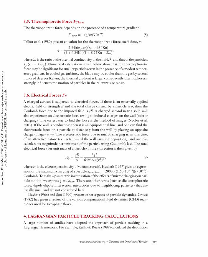
(Friedlander & Johnstone 1957, Liu & Agarwal 1974, McCoy & Hanratty 1977, Wells& Chamberlain 1967). Although there is considerable scatter, these data illustrate thebasic characteristics shown in Figure 1. The results fall into three distinct categories:(a) At first, as τ+ increases, the deposition velocity decreases. This is the so-calledturbulent diffusion regime, in which a turbulent version of Fick’s law of diffusion (seebelow) applies. (b) The striking feature of the next zone, the so-called eddy diffusion-impaction regime, is that the deposition velocity increases by three to four ordersof magnitude. (c) The third regime of deposition, usually termed the particle inertiamoderated regime, results in an eventual decrease in the deposition velocity for largeparticle sizes. The borders between the three regimes are not sharp, as one effectgradually merges into another, and depend on flow conditions.
log10 (τ+)
Small particles Large particles
–2 –1 0 1 2 3–6
–5
–4
–3
–2
–1
0
1 2 3
Fick’s law of diffusionis applicable here
log
10 (V
dep
)+
Figure 1A typical variation inmeasured deposition ratewith particle relaxation timein fully developed verticalpipe flow. Regime 1,turbulent diffusion; regime2, turbulent diffusion-eddyimpaction; regime 3,particle inertia moderated.
www.annualreviews.org • Transport and Deposition of Particles 313
Ann
u. R
ev. F
luid
Mec
h. 2
008.
40:3
11-3
41. D
ownl
oade
d fr
om a
rjou
rnal
s.an
nual
revi
ews.
org
by U
nive
rsity
of
Lau
sann
e on
05/
19/0
8. F
or p
erso
nal u
se o
nly.
ANRV332-FL40-14 ARI 10 November 2007 16:27
2.1. Molecular and Turbulent Diffusion
Most mass-transfer textbooks (e.g., Kay & Nedderman 1988) show that one cancalculate the flux of small particles in a turbulent boundary layer by integrating amodified Fick’s law of diffusion,
J = −(DB + Dt)dρp
dy, (2)
where DB is the Brownian diffusivity; Dt is the turbulent diffusivity, which varieswith position; y is the perpendicular distance from the wall; and dρp
dy is the gradientof particle partial density (same as concentration gradient). DB is given by the Ein-stein equation incorporating Cunningham’s (1910) correction (CC = 1 + 2.7Kn) forrarefied gas effects,
DB =(
kT6πμr
)CC , (3)
where k is the Boltzmann constant, T is the absolute temperature, and Kn is theKnudsen number defined by Kn = l/2r, where l is the mean free path of the sur-rounding gas and r is the radius of a particle. Another semiempirical form for theCunningham factor, CC = 1 + Kn[a + b exp(−c /Kn)], is also widely used: Davies(1945) gave the values of the constants as a = 2.514, b = 0.8, and c = 0.55. Slightlydifferent values for these constants are sometimes used in the literature. Equation 3shows that DB decreases with increasing r. Equation 2 therefore predicts that themass flux of particles and deposition velocity decrease continuously with increasingparticle size. Figure 1 shows a more complex behavior, and Fick’s law does not givea complete description. We describe in the following sections both Lagrangian andEulerian computational methods to illustrate what happens in the second and thirdregimes of deposition velocity.
3. PARTICLE MOTION AND VARIOUS FORCES
This section describes a few common forces that affect particle motion. The magni-tudes of various forces are expressed as those per unit mass of the particle (becauseboth Eulerian and Lagrangian schemes are conveniently expressed in terms of particleacceleration). The following equations contain vector quantities; hence magnitudesand directions need to be accounted for properly. The effects of virtual mass andthe Basset history term (Maxey & Riley 1983) are usually not included in depositionstudies—both these terms are small when the ratio of particle material density andfluid density is large (ρ0
p/ρ � 1), a condition generally satisfied for the motion ofsolid particles or liquid droplets in a gas.
3.1. Aerodynamic Drag FD
A particle moving in a fluid experiences a drag force. The drag force is alwayspresent, and it acts as a mechanism by which a particle tries to catch up with thechanging velocities of the surrounding fluid (for discussions on the physical aspectsof relaxation phenomena, see Becker 1970; Guha 1995, 2007). The drag force FD
314 Guha
Ann
u. R
ev. F
luid
Mec
h. 2
008.
40:3
11-3
41. D
ownl
oade
d fr
om a
rjou
rnal
s.an
nual
revi
ews.
org
by U
nive
rsity
of
Lau
sann
e on
05/
19/0
8. F
or p
erso
nal u
se o
nly.
ANRV332-FL40-14 ARI 10 November 2007 16:27
(per unit mass of the particle) may generally be expressed as
FD = Vf − Vp
τ, (4)
where Vf and Vp are fluid and particle velocities, respectively. The equation appliesto instantaneous as well as time-mean values. For spherical particles with small slipvelocity (�V = Vf −Vp ), the magnitude of the drag force is given by the Stokes result,FD = 6π rμ|�V|/m, where m is the mass of an individual particle (m = 4
3 πr3ρ0p ,
where ρ0p is the density of pure particulate material). Inserting this result into
Equation 4, one finds that in the Stokes drag regime τ is given by
τ = 2ρ0pr2/9μ. (5a)
The curves for the variation of V+dep versus τ+ are plotted with this definition of the
relaxation time. However, in the numerical calculations, one needs to correct therelaxation time to account for the slip velocity for large particles and the rarefied gaseffects for very small particles. The rarefied gas effects can be modeled by the Cun-ningham correction factor CC as used in Equation 3, whereas the effects of a large slipReynolds number are modeled by incorporating an empirical particle drag coefficient,CD. The general expression for the inertial relaxation time τI is then given by
τI = τ24
ReCDCC , (5b)
where Re is the slip Reynolds number defined as Re = 2r |�V|/ν, and CD is a functionof Re. Morsi & Alexander (1972) give an empirical equation that is widely used: CD =a1 + a2/Re + a3/Re2, where the values of a1, a2, and a3 are provided in several piece-wise ranges of Re. Another much used equation is CD = (24/Re)(1 + 0.15Re0.687);Clift et al. (1978) attribute this equation to Schiller and Nauman, dating back to 1933.
The aerodynamic drag for nonspherical particles is usually expressed as an em-pirical correction to the drag of equivalent spheres by introducing suitable shapefactors. Various geometric shape factors for a particle of an arbitrary shape are pro-posed by combining two of the four quantities: volume, surface area, projected area,and projected perimeter. For example, a widely used volumetric shape factor is cal-culated as volume/(4 × projected area/π )3/2. Theoretical and experimental values ofthe drag are more readily available for regular nonspherical shapes (e.g., spheroidal,cylindrical) than for arbitrary shapes, and these values are given by Clift et al. (1978).Different orientations and the possible rotation of nonspherical particles add to thecomplexity.
Sometimes the concept of an aerodynamic diameter (dae) is used, which is thediameter of a unit density sphere (usually taken as 1 g cm−3) that has the same gravi-tational settling speed as the particle in question (aerodynamic drag is therefore thesame at the terminal speed). The aerodynamic diameter is given by dae = dV
√ρ0
p/SD,where dV is the diameter of an equivalent spherical particle that has the same vol-ume as the nonspherical particle in question, and SD is the dynamic shape correctionfactor. Hinds (1999) gives values for SD for common geometric shapes and particletypes.
www.annualreviews.org • Transport and Deposition of Particles 315
Ann
u. R
ev. F
luid
Mec
h. 2
008.
40:3
11-3
41. D
ownl
oade
d fr
om a
rjou
rnal
s.an
nual
revi
ews.
org
by U
nive
rsity
of
Lau
sann
e on
05/
19/0
8. F
or p
erso
nal u
se o
nly.
ANRV332-FL40-14 ARI 10 November 2007 16:27
3.2. Inertial Impaction
If the magnitude and direction of the fluid velocity (mean velocity in the contextof turbulent flow) change rapidly, significant velocity slip may develop (as shown inEquation 4), particularly for larger particles. When the fluid time-mean streamlinesare curved, particles may not be able to follow them as a result of inertia, and thedeviated particle pathlines may make them collide with nearby solid walls and getdeposited, which is known as inertial impaction. This may be an important mech-anism, for example, for the highly curved blades in steam and gas turbines or forthe complex flow passages with rapid turning in the nasopharyngeal region of thehuman respiratory tract or in the branching bronchial tree. Inertial impaction maybe relevant for either laminar or turbulent flow.
3.3. Gravitational Force FG
A particle in a gravitational field experiences a force (weight) in the direction of thegravitational acceleration g. The particle also experiences a force in the oppositedirection (buoyancy), which, according to the Archimedes principle, is equal to theweight of the displaced fluid. Hence, the net gravitational force (per unit mass ofparticle), FG, is given by
FG =(
1 − ρ
ρ0p
)g. (6)
In situations in which gravity and aerodynamic forces are balanced, a particle acquiresa terminal speed known as the gravitational settling speed, Vgs . One can determinethe magnitude of the gravitational settling speed from Equations 4 and 6: Vgs =(1 − ρ/ρ0
p )gτI . In noninertial reference frames, centrifugal forces may give rise tosimilar body force effects like gravity.
3.4. Shear-Induced Lift Force FS
Saffman (1965, 1968) provided an expression for the shear-induced lift force, which(per unit mass and in the y direction) is
FSy = 1.542ρ
ρ0pν
1r
√1ν
∣∣∣∣d V̄f x
dy
∣∣∣∣ (V̄f x − V̄px). (7)
Calculations show that the effect of FS is usually to enhance deposition velocity.The majority of deposition calculations reported in the literature make use of theSaffman expression for the lift force. However, Saffman originally derived his resultfor an unbounded shear flow. For deposition calculations, one should use modifiedexpressions for the lift force that include the effects of the proximity of a wall andfinite Reynolds numbers. The sign of the Saffman lift force in a particular directiondepends on the sign of the slip velocity in the perpendicular direction. Guha (1997,appendix B) discusses a subtle interaction between FS, gravity, and particle convectivevelocity toward a wall in vertical flow.
316 Guha
Ann
u. R
ev. F
luid
Mec
h. 2
008.
40:3
11-3
41. D
ownl
oade
d fr
om a
rjou
rnal
s.an
nual
revi
ews.
org
by U
nive
rsity
of
Lau
sann
e on
05/
19/0
8. F
or p
erso
nal u
se o
nly.
ANRV332-FL40-14 ARI 10 November 2007 16:27
3.5. Thermophoretic Force FTherm
The thermophoretic force depends on the presence of a temperature gradient:
FTherm = −(η/m)∇ ln T. (8)
Talbot et al. (1980) give an equation for the thermophoretic force coefficient, η:
η = 2.34(6πμνr)(λr + 4.36Kn)(1 + 6.84Kn)(1 + 8.72Kn + 2λr )
,
where λr is the ratio of the thermal conductivity of the fluid, λ, and that of the particles,λp (λr = λ/λp ). Numerical calculations given below show that the thermophoreticforce may be significant for smaller particles even in the presence of a modest temper-ature gradient. In cooled gas turbines, the blade may be cooler than the gas by severalhundred degrees Kelvin; the thermal gradient is large; consequently thermophoresisstrongly influences the motion of particles in the relevant size range.
3.6. Electrical Forces FE
A charged aerosol is subjected to electrical forces. If there is an externally appliedelectric field of strength E and the total charge carried by a particle is q, then theCoulomb force due to the imposed field is qE. A charged aerosol near a solid wallalso experiences an electrostatic force owing to induced charges on the wall (mirrorcharging). The easiest way to find the force is the method of images (Nadler et al.2003). If the wall is conducting, then it is an equipotential line, and one can find theelectrostatic force on a particle at distance y from the wall by placing an oppositecharge (image) at –y. The electrostatic force due to mirror charging is, in this case,of an attractive nature (i.e., acts toward the wall assisting deposition), and one cancalculate its magnitude per unit mass of the particle using Coulomb’s law. The totalelectrical force (per unit mass of a particle) in the y direction is then given by
FEy = qEm
− 3q 2
64π2ε0ρ0pr3 y2
, (9)
where ε0 is the electric permittivity of vacuum (or air). Hesketh (1977) gives an expres-sion for the maximum charging of a particle qmax: qmax = 2000×(1.6×10−19)(r/10−6)2
Coulomb. To make a parametric investigation of the effects of mirror charging on par-ticle motion, we express q = ξqmax. There are other terms (such as dielectrophoreticforce, dipole-dipole interaction, interaction due to neighboring particles) that areusually small and are not considered here.
Davies (1966) and Soo (1990) present other aspects of particle dynamics. Crowe(1982) has given a review of the various computational fluid dynamics (CFD) tech-niques used for two-phase flows.
4. LAGRANGIAN PARTICLE TRACKING CALCULATIONS
A large number of studies have adopted the approach of particle tracking in aLagrangian framework. For example, Kallio & Reeks (1989) calculated the deposition
www.annualreviews.org • Transport and Deposition of Particles 317
Ann
u. R
ev. F
luid
Mec
h. 2
008.
40:3
11-3
41. D
ownl
oade
d fr
om a
rjou
rnal
s.an
nual
revi
ews.
org
by U
nive
rsity
of
Lau
sann
e on
05/
19/0
8. F
or p
erso
nal u
se o
nly.
ANRV332-FL40-14 ARI 10 November 2007 16:27
of particles in a simulated turbulent fluid field; Ounis et al. (1993) and Brooke et al.(1994) computed the motion of particles for which the fluid motion was determinedby DNS of the Navier-Stokes equations; Wang & Squires (1996) solved the fluidvelocity field using large eddy simulation; and Fichman et al.’s (1988) and Fan &Ahmadi’s (1993) calculations were based on the sublayer approach originally pro-posed by Cleaver & Yates (1975).
In the particle tracking methods, the momentum equation for the particle is writ-ten and then integrated with respect to time along the particle pathline. Typicallythe motion of a very large number of particles is solved, and from this one can con-struct statistically meaningful ensemble average quantities. The particle momentumequation and position equation in the i direction can be written on the basis of thediscussions in Section 3:
d Vpi
dt= Vfi − Vpi
τI+ FGi + FSi + FTherm,i + FEi + Bi , (10)
dxi
dt= Vpi. (11)
Equations 10 and 11 can be numerically integrated together, giving the new positionand velocity at the end of each computational time step. It is straightforward to includeother forces not considered here in Equation 10.
The first and last terms in the right-hand side of Equation 10 deserve special men-tion. If one wants to calculate the impact of fluid turbulence on the particle motion,one must use the instantaneous fluid velocity Vf in the first term. If one uses thetime-mean value V̄f in the first term, no matter what sophisticated turbulent calcu-lation method was used in determining it, proper turbulent diffusion and dispersioncharacteristics of particles are not captured. The average particle motion calculatedby first determining the time-mean fluid velocity and then using Lagrangian trackingthrough this steady fluid flow field is not the same as first using Lagrangian trackingthrough a fluctuating fluid flow field and then averaging. Of course, if time-mean V̄f
is used, some particle dispersion and deposition may still be predicted if other mecha-nisms such as inertial impaction (see Section 3.2) or gravitational settling (Section 3.3)are present, as they would be in a laminar flow. Under certain combinations of flowgeometry and particle size, these other mechanisms can even be the dominant factors(but one needs to be aware of these considerations, particularly when using CFDpackages to perform Lagrangian particle tracking with time-mean V̄f ). The fluctuat-ing turbulent field may also alter the steady-state values of other forces in Equation10, such as FS, but such effects are considered small and usually are not includedin reported studies. The last term in Equation 10 represents the Brownian forceon a particle and must be included especially for small particles (see regime 1 inFigure 1).
The attraction of the Lagrangian tracking method is obvious, and the form ofEquation 10 is general and direct. The coding of the computer program is relativelysimple (as compared with the coding of an Eulerian method). The interactions ofparticles with the solid boundary (e.g., rebounding) can also be modeled in a simplemanner. A polydispersed droplet population, even when a change in particle size is
318 Guha
Ann
u. R
ev. F
luid
Mec
h. 2
008.
40:3
11-3
41. D
ownl
oade
d fr
om a
rjou
rnal
s.an
nual
revi
ews.
org
by U
nive
rsity
of
Lau
sann
e on
05/
19/0
8. F
or p
erso
nal u
se o
nly.
ANRV332-FL40-14 ARI 10 November 2007 16:27
involved, can be accommodated easily. When the particle inertia is very large andthe fluid flow field has significant streamline curvature (such that inertial impactionand/or gravitational settling is the dominant mechanism), then a picture of the par-ticle velocity field and deposition can be built from the Lagrangian tracking of areasonably small number of particles through the time-mean fluid flow field—suchcalculations can be relatively inexpensive. Hence, often in the literature one findsmixed Eulerian-Lagrangian calculations in which the mean fluid field in complexthree-dimensional geometry is calculated by Eulerian methods, and then Lagrangiancalculations are performed on particles. Most commercial CFD codes have this facil-ity. However, if calculation of the particle concentration field is also necessary (e.g.,Marchioli & Soldati 2002) in addition to the particle velocity field, then Lagrangiancalculations face challenges and can be computationally expensive. Moreover, whenparticle motion is significantly influenced by fluid turbulence, then Lagrangian cal-culations with fluctuating fluid velocity are needed (the fluid field being determinedby Reynolds-averaged Navier-Stokes, large eddy simulation, or DNS). Such trackingcalculations are typically performed for a large number of particles (may be 104, 105,or many more) for statistically meaningful results, and the computational time stepneeded is small (particularly for small particles for which Brownian diffusion may alsoneed to be included); hence stochastic Lagrangian calculations are computationallyintensive and expensive. The method can thus be a good research tool for understand-ing the flow physics, but it is unlikely to become a practical method for engineeringcalculations or be used as a design tool.
4.1. Stochastic Eddy Interaction Models
The instantaneous turbulent fluid velocity may be computed directly by a DNS ap-proach. Often, instead a Monte Carlo simulation (also known as random walk mod-eling in this context) is performed. In this approach, a particle’s stochastic trajectoryis modeled as a succession of interactions with turbulent eddies. The time-meanfluid velocity V̄f is calculated by a suitable turbulent computational method (e.g., thek − ε model). A simulated fluctuating velocity field is then superposed to calculatethe instantaneous fluid velocity (Vf = V̄f + V ′
f ). A fluid eddy is assigned a fluctuatingvelocity V ′
f , which is assumed to stay constant during the lifetime of the eddy te. Asa particle encounters an eddy on its pathline, Equations 10 and 11 are integratedtogether to calculate the particle velocity and position at the end of the particle res-idence time tr . Small particles usually stay within the same eddy during the eddy’slifetime (then tr = te ); particles with large inertia may leave the eddy before the eddydecays (in this case, tr < te ). Once the particle has left the eddy or the eddy lifetime isover, the particle encounters a new eddy at its current location, and the integration ofEquations 10 and 11 is repeated in the same manner. The calculation for a particle iscontinued until the particle is captured by a wall (deposition has then taken place) orgoes out of the computational space. The calculation procedure is repeated for manyparticles.
The differences between the various reported schemes are mainly in how the ve-locity scale, length scale, and eddy lifetime are generated and randomized. An adopted
www.annualreviews.org • Transport and Deposition of Particles 319
Ann
u. R
ev. F
luid
Mec
h. 2
008.
40:3
11-3
41. D
ownl
oade
d fr
om a
rjou
rnal
s.an
nual
revi
ews.
org
by U
nive
rsity
of
Lau
sann
e on
05/
19/0
8. F
or p
erso
nal u
se o
nly.

ANRV332-FL40-14 ARI 10 November 2007 16:27
scheme should preserve the dispersion characteristics of the original turbulent flowand needs to be validated for this purpose. The method used for calculating the eddylifetime and eddy length scale determines the Lagrangian and Eulerian autocorrela-tion, respectively.
Usually these stochastic models calculate the eddy velocity as V ′f = NGvrms , where
vrms is the root mean square (rms) of the fluid fluctuating velocity in the relevantdirection, and NG is a random number drawn from a Gaussian probability densitydistribution of zero mean and unity standard deviation. Another probability densityfunction other than the Gaussian can also be used. If a constant eddy life is used inthe simulation, then it should be chosen such that te = 2TL, where TL is the fluidLagrangian integral time scale, to preserve the long-term dispersion characteristics;random time steps should be used to produce a smooth Lagrangian autocorrelationfunction (Wang & Stock 1992). Similarly, if a constant eddy length scale (le) is used,then it should be chosen such that le = 2LE , where LE is the Eulerian integral lengthscale (Graham & James 1996). For (solid) particles with finite inertia, the Lagrangianintegral time scale for the particle lies between the Lagrangian and Eulerian integraltime scales for the fluid.
Gosman & Ioannides (1983) used a k − ε method for calculating the time-meanfluid velocity field, assumed isotropic fluctuating velocities (vrms ,i = √
2k/3), andcalculated the eddy length scale from le = C0.5
μ k1.5/ε and eddy time scale fromte = le/|V ′
f |. Hutchinson et al. (1971) used a constant te. Shuen et al. (1983) used thesame model as Gosman & Ioannides (1983) except they used te = le/(
√2k/3). Kallio
& Reeks (1989) simulated the turbulent fluid velocity field using empirical curve fit-tings for the time-mean x velocity V̄f,x , rms y fluctuations vrms ,y , and Lagrangian timescale TL, all as functions of the wall coordinate y+. The particle residence time wastaken to be always equal to the eddy lifetime (tr = te ); hence they need not specifythe eddy length scale (le). The eddy time scale (te) was calculated by randomizing theLagrangian integral time scale TL from an exponential probability density distribu-tion. Berlemont et al. (1990) provided another approach for stochastic Lagrangiancalculation. This method uses a correlation matrix in the random process to explicitlyspecify any shape of the Lagrangian correlation function.
Kallio & Reeks’s (1989) study is important in terms of deposition calculationsbecause (despite its inability to capture regime 1 in Figure 1 as a result of ignoringBrownian movement) it showed that a simple stochastic theory could predict thegeneral behavior of particle deposition in regimes 2 and 3 in Figure 1.
4.2. Markov Chain–Type Turbulent Random Walk Models
There are many papers on this approach particularly developed in the context ofatmospheric dispersion (Durbin 1980, Luhar & Britter 1989, Sawford 1982, Walklate1987). Whereas for the stochastic eddy interaction models the Lagrangian velocitiesare generated through independent random numbers, for the Markov chain–typesimulations the velocities are generated through dependent random numbers withone-step memory. For a one-dimensional case, if x(t) and v f (t) are the position andvelocity, respectively, of a fluid particle or a tracer particle, then the evolution of
320 Guha
Ann
u. R
ev. F
luid
Mec
h. 2
008.
40:3
11-3
41. D
ownl
oade
d fr
om a
rjou
rnal
s.an
nual
revi
ews.
org
by U
nive
rsity
of
Lau
sann
e on
05/
19/0
8. F
or p
erso
nal u
se o
nly.
ANRV332-FL40-14 ARI 10 November 2007 16:27
(v f , x) is generally described as
dv f = a(x, v f ) dt + √(C0ε) dξ, (12a)
d x = v f d t, (12b)
where dξ is a random velocity increment of the Wiener process with zero mean andvariance dt, C0 is a universal constant (Monin & Yaglom 1975), and ε is the meanrate of dissipation of turbulent kinetic energy. The function a is determined by solv-ing a Fokker-Planck equation to satisfy the well-mixed criterion (Thomson 1987),which ensures that a globally uniform source of tracer is not unmixed by the tur-bulent motions. For the homogeneous, isotropic, stationary case, a = −v f /TL andC0ε = 2v2
rms /TL, and Equation 12a becomes the basic Langevin equation. It is usuallystated that dt should be less than 0.1TL, so that the effect of the size of computationaltime step does not significantly affect the Lagrangian velocity correlation. Applica-tion of this type of random walk model can be complex in strongly inhomogeneousand anisotropic turbulent flow, in multidimensional dispersion problems, and whenparticle inertia is significant.
4.3. Calculation of the Brownian Force Bi
One can adopt a molecular dynamics approach to calculate Brownian movement.However, in the context of the discussion on the stochastic simulation of turbulencein the previous two sections above, one could either alter the expression for thedisplacement in the Markov chain process (Borgas & Sawford 1996) or add a force(e.g., Ounis et al. 1993) in the eddy interaction model. In the Markov chain approach,the form of Equation 12a remains the same, but Equation 12b is replaced by d x =v f d t + √
2DBdξ ′, where dξ ′ is a random number representing white noise, and theBrownian diffusion coefficient DB is given by Equation 3.
In the eddy interaction model, the Brownian force (per unit mass of particle) in
each direction is specified as a Gaussian white noise: Bi = (NGi/m)√
(2k2T2f )/(DB�t),
where �t is the computational time step, and NGi is a Gaussian random number withzero mean.
5. EULERIAN PARTICLE TRANSPORT CALCULATIONS
All practical CFD computations for a single-phase fluid in complex geometries areperformed in the Eulerian framework. Hence, it is profitable to solve the particleequations in the same way for easy integration with the established CFD codes forthe primary fluid. The Eulerian-Eulerian calculations are computationally efficient(compared with stochastic Lagrangian tracking calculations) and hence are neces-sary for engineering calculations and as a design tool. However, turbulence closureproblems have to be tackled. There are also challenges in implementing physicallycorrect treatment at solid boundaries, including particle rebounding. Crossing trajec-tories, discontinuities in concentration, and polydispersed particle cloud with tempo-ral change in size of an individual particle (e.g., due to condensation or evaporation;
www.annualreviews.org • Transport and Deposition of Particles 321
Ann
u. R
ev. F
luid
Mec
h. 2
008.
40:3
11-3
41. D
ownl
oade
d fr
om a
rjou
rnal
s.an
nual
revi
ews.
org
by U
nive
rsity
of
Lau
sann
e on
05/
19/0
8. F
or p
erso
nal u
se o
nly.

ANRV332-FL40-14 ARI 10 November 2007 16:27
see Guha 1994, 1995, 1998a; Guha & Young 1991) further complicate thematter.
Historically, it was Eulerian modeling that was first applied to calculate particledeposition in the second regime (regime 2 of Figure 1). Starting with Friedlander& Johnstone’s (1957) landmark paper, this genre of calculations, variously called stopdistance or free flight models, has been used in engineering solutions for a longtime. Although these models have contributed strongly to the development of ourunderstanding of deposition, they have fundamental difficulties. Whereas this classof models tried to capture the physics of deposition by solving the particle conti-nuity equation alone, in the past 15 or so years Eulerian computational methods ofdeposition have been developed that solve both particle continuity and momentumequations ( Johansen 1991, Guha 1997, Young & Leeming 1997). These models showthat the interaction of particle inertia and the inhomogeneity of fluid turbulent flowfield (in the boundary layer close to a solid surface) gives rise to a new mechanismof particle transport called turbophoresis (Caporaloni et al. 1975, Reeks 1983). Tur-bophoresis (in which particle transport is caused by gradients in fluctuating velocities)is a separate effect and must be treated as such; it cannot be properly reproduced byany tuning of the theoretical model for diffusion (which is driven by the gradientsin concentration). Turbophoresis is not a small correction to Fick’s law of diffusion;Guha (1997) showed that it is the primary mechanism operative in regimes 2 and 3 ofFigure 1. Guha (1997) further demonstrated that for large particles, the momentumequation alone can provide nearly accurate estimates of the deposition velocity; theabsence of the use of the particle momentum equation in the stop distance models istherefore their major weakness. Theoretical treatments on particle motion in turbu-lent flow, including kinetic approaches, are given by Reeks (1977, 1991, 1992), Rizk& Elghobashi (1985), Simonin et al. (1993), and Zaichik (1999), among others.
5.1. Stop Distance or Free Flight Models
One of the most used Eulerian calculation methods has been the free flight orstop distance model (e.g., Beal 1970, Davies 1966, Friedlander & Johnstone 1957,Papavergos & Hedley 1984, Wood 1981). These models assume that particles diffuseto within one stop distance, s, from the wall, at which point they make a free flightto the wall. The main difference between different models of this type lies in theprescription of the free flight velocity, vff. A simple integration of Equation 4 showsthat, in nondimensionalized form, s + = (vff/u∗)τ+. Friedlander & Johnstone (1957)assumed vff = 0.9u∗, a value close to the fluid rms velocity in the outer layer of aturbulent boundary layer. Their model agrees well with experiments in a vertical pipe(in the second regime). Davies (1966) made an apparently more plausible assumptionthat the free flight velocity is the same as the local rms velocity of the fluid at the pointat which the particle starts its free flight, but his calculated deposition velocities wereapproximately two orders of magnitude lower than the experimental values. Liu &Ilori (1974) improved the prediction of this model by prescribing, rather arbitrarily,a particle diffusivity that was different from the commonly used eddy momentumdiffusivity. Beal (1970) gave another variation of the stop distance model.
322 Guha
Ann
u. R
ev. F
luid
Mec
h. 2
008.
40:3
11-3
41. D
ownl
oade
d fr
om a
rjou
rnal
s.an
nual
revi
ews.
org
by U
nive
rsity
of
Lau
sann
e on
05/
19/0
8. F
or p
erso
nal u
se o
nly.
ANRV332-FL40-14 ARI 10 November 2007 16:27
These models, although significantly contributing to the development of ourunderstanding, are physically not satisfactory. The stop distance models predict amonotonic rise in stopping distance (which may exceed the buffer layer thickness ofa turbulent boundary layer for larger particles because s + ∼ τ+) and consequentlypredict a monotonic increase in deposition velocity with increasing τ+. Experiments,however, show a third regime of deposition, usually termed the particle inertia mod-erated regime, in which the deposition velocity decreases with a further increase inτ+ (see Figure 1). Stop distance models are not of much use here, and new theories(e.g., Reeks & Skyrme 1976) need to be applied.
Thus, even for the apparently simple case of turbulent deposition in a fully de-veloped pipe flow, a separate theory had to be applied for each deposition regime.Although it is possible, with proper tuning of the models (e.g., by prescribing the freeflight velocity), to partially reproduce the experimental results for fully developedpipe flow, the theories cannot be extrapolated to two- or three-dimensional flow sit-uations with any great confidence because of their piecemeal nature and the requiredempirical tuning. Additionally, when other effects such as thermophoresis or electro-static interaction are present, the stop distance models would need postulations suchas that the deposition velocities due to various mechanisms calculated separately canbe simply added (linear superposition).
5.2. A Unified Advection-Diffusion Theory
Guha (1997) has established, by deriving from the fundamental Eulerian conserva-tion equations of mass and momentum for the particles, a unified advection-diffusiontheory in which turbophoresis arises naturally. The theory includes molecular andturbulent diffusion, thermophoresis, shear-induced lift force, electrical forces, andgravity. It incorporates the effects of surface-roughness elements and particle inter-ception. The framework is general, and the theory can be integrated efficiently withestablished multidimensional CFD codes for single-phase flow. The theory reducesto Fick’s law of diffusion in the limit of small particles, thus linking Fick’s law to abroader scheme of particle transport. The prediction of deposition velocity from thisEulerian theory is at least as accurate as those from the state-of-the-art Lagrangiancalculations, including DNS studies, but the Eulerian computation is much faster(and the inclusion of Brownian diffusion is simple).
The new Eulerian theory uses Ramshaw’s (1979) approach to model the forceson a particle in a flowing fluid stream, in particular how the Brownian diffusion ismodeled (see also Fernandez De La Mora & Rosner 1982). Various flow variables(such as fluid and particle velocity, particle partial density) are decomposed into theirmean and fluctuating parts, and then the particle continuity and momentum conser-vation equations are Reynolds averaged. The resulting equations are then simplified,identifying and retaining the dominant terms, so that clear physical meaning could beascribed to each term. The equations given in Guha (1997) are general and can, forexample, be used to study particle deposition in a developing boundary layer. Here,only the equations for fully developed, vertical flow are discussed to bring out theessential flow physics.
www.annualreviews.org • Transport and Deposition of Particles 323
Ann
u. R
ev. F
luid
Mec
h. 2
008.
40:3
11-3
41. D
ownl
oade
d fr
om a
rjou
rnal
s.an
nual
revi
ews.
org
by U
nive
rsity
of
Lau
sann
e on
05/
19/0
8. F
or p
erso
nal u
se o
nly.
ANRV332-FL40-14 ARI 10 November 2007 16:27
If the flux of particles in the y direction (which is perpendicular to the solid wall)is denoted by J, then the Reynolds averaging of the particle continuity equation forfully developed flow gives
∂J/∂y = 0,
where
J = −(DB + Dt)∂ρ̄p
∂y− DT ρ̄p
∂ ln T∂y
+ ρ̄p V̄cpy, (13)
where DT is the coefficient of diffusion due to temperature gradient, and V̄cpy is the
particle convective velocity in the y direction. Any quantity with an overbar denotesits time-mean value. DT is given by
DT = DB (1 + η/kT ). (14)
Equation 14 shows that the thermal drift has a stressphoretic component and a ther-mophoretic component (the term containing η). The stressphoretic component arisesfrom the evaluation of ∇ p p , where p p is the partial pressure of a hypothetical idealgas consisting of the particle cloud (Ramshaw 1979).
Equation 13 is the generalized equation for particle flux. The particle convectivevelocity in the y direction, V̄c
py, has to be calculated from the particle momentumequation. The Reynolds-averaged particle momentum equations in the y and xdirections, slightly simplified and specialized for fully developed vertical flow, are
y momentum: V̄cpy
∂ V̄cpy
∂y+ V̄c
py
τI= −∂V ′2
py
∂y+ FSy + FEy, (15a)
x momentum: V̄cpy
∂ V̄px
∂y= 1
τI(V̄fx − V̄px) + (
1 − ρ f /ρ0p
)g. (15b)
In Equation 15a, V̄cpy
∂ V̄cpy
∂y is the acceleration term,V̄c
pyτI
is the steady-state viscous drag(simplified with the assumption V̄fy = 0), − ∂V ′2
py∂y is the turbophoresis, FSy is the shear-
induced lift force, and FEy is the electrical force. Equation 15b represents downwardflow; for upward flow, one should replace g with –g. Note that the x momentum(Equation 15b) involves both V̄px and V̄c
py. The y momentum (Equation 15a) is, how-ever, almost decoupled and depends on V̄px only through the shear-induced lift force,FSy. A study of Equations 15a and 15b also shows nicely how gravity affects they-momentum equation through the lift force. The left-hand side of Equation 15b in-volves V̄c
py. As a result of this convective velocity in the y direction, the direction of thelift force may remain unaltered whether the flow is vertically downward or upward.
In the general case, both Equations 15a and 15b must be solved simultaneously.Calculations show that the shear-induced lift force increases the deposition rate,particularly in the eddy diffusion-impaction regime. The effect of the lift force, FSy,is not considered below. With these provisos, V̄c
py can be calculated from
V̄cpy
ddy
(V̄c
py
)+ V̄c
py
τI= − d
dy
(V ′2
py
)+ FEy. (15c)
The second term on the left-hand side of Equation 15c is the steady-state drag sim-plified with the assumption V̄f y = 0; the full form is −(V̄f y − V̄c
py)/τI . The first term
324 Guha
Ann
u. R
ev. F
luid
Mec
h. 2
008.
40:3
11-3
41. D
ownl
oade
d fr
om a
rjou
rnal
s.an
nual
revi
ews.
org
by U
nive
rsity
of
Lau
sann
e on
05/
19/0
8. F
or p
erso
nal u
se o
nly.
ANRV332-FL40-14 ARI 10 November 2007 16:27
on the right-hand side of Equation 13 is the diffusion due to a gradient in the particleconcentration (same as Fick’s law given by Equation 2); the second term representsthe diffusion due to a temperature gradient; and the third term represents a convectivecontribution arising owing to particle inertia. Equation 15c relates the particle con-vective velocity with the gradient in turbulence intensity (turbophoresis) and otherexternal forces. It is chiefly the absence of this convective term in Fick’s law thatnecessitated postulating stop distance or free flight models. From Equation 15c, onecan write the expression for turbophoretic velocity (Vp,turbo ) as Vp,turbo = τI [− d
dy (V ′2py )].
Importantly, the turbophoretic term depends on the particle rms velocity which maybe different from the fluid rms velocity if the particle inertia is large (see Equation 17).When the particles are very small, they effectively follow the fluid eddies, and thetwo rms velocities are essentially the same. In this limit, τI → 0, the expression forturbophoretic velocity then shows that Vp,turbo → 0. Turbophoresis is thus negli-gible for small particles even if there exists a gradient in fluid turbulence intensity.Fick’s law is, therefore, an adequate description for the deposition of small particles.As τI increases, the turbophoretic term assumes dominance, thereby increasing thedeposition rate by a few orders of magnitude. However, as τI increases, the particlesare less able to follow fluid fluctuations, and the particle rms velocity becomes pro-gressively smaller as compared with the fluid rms velocity. This is one of the factorsresponsible for the eventual decrease in deposition velocity with increasing particlesize when τI is very large. The turbophoretic velocity vanishes (Vp,turbo = 0), for allparticles irrespective of the particle inertia, when the flow is either not turbulent orwhen the turbulence is homogenous [∂/∂y(V ′2
fy ) = 0]. However, even in laminar flow,Equations 13 and 15 apply and can predict all such effects like Brownian diffusion,thermophoresis, and convective slip velocity due to streamline curvature and externalbody forces such as gravity or electrical interactions.
For not too large particles, the steady-state drag term (second term on the left-hand side of Equation 15c) almost balances the turbulence term (right-hand side),and the acceleration term (first term on left-hand side) is negligible. The accelera-tion term assumes importance for large particles and should not be neglected: It isthe chief reason why the deposition velocity eventually decreases in the third regime(see Figure 1). Neglecting the acceleration term would predict a constant depositionvelocity at large τ+. [Interestingly, such constancy in deposition velocity is character-istic of some of the previous calculations; even Fan & Ahmadi’s (1993) Lagrangiancalculations show this behavior.]
The unified advection-diffusion theory is logical in finding the combined effectsof different particle transport mechanisms, as the appropriate forces are added inthe momentum equation, and the combined velocity or flux is calculated directlyby solving the continuity and momentum equations. This should be superior tothe often-used linear addition of respective velocities, each calculated separately, todetermine the combined mass flux.
Fluid and particle root-mean-square velocities. Equations 13–15 would workwell if one could find an accurate expression for the particle rms velocity as a func-tion of the wall coordinate. The variation of fluid rms velocity as a function of wall
www.annualreviews.org • Transport and Deposition of Particles 325
Ann
u. R
ev. F
luid
Mec
h. 2
008.
40:3
11-3
41. D
ownl
oade
d fr
om a
rjou
rnal
s.an
nual
revi
ews.
org
by U
nive
rsity
of
Lau
sann
e on
05/
19/0
8. F
or p
erso
nal u
se o
nly.
ANRV332-FL40-14 ARI 10 November 2007 16:27
coordinate can be determined from measurements (Bremhorst & Walker 1973,Finnicum & Hanratty 1985, Kreplin & Eckelmann 1979, Laufer 1954), near-wallmodeling work (Chapman & Kuhn 1986), and DNS (Kim et al. 1987). Kallio &Reeks (1989) have given an empirical curve fit for the region 0 < y+ < 200 (thisequation is quoted below after correcting errors in the original paper):√
(V ′+f y )2 = 0.005y+2/(1 + 0.002923y+2.128). (16)
Accurate prediction of fluid rms velocity is important. Other equations with piecewisecontinuous (and differentiable) curve fits can be used, if deemed appropriate.
It is possible to relate the particle mean square velocity to the fluid mean squarevelocity through a parameter , which is defined as the ratio of the two:
= V ′2py /V ′2
f y . (17)
It is difficult to devise a simple but accurate mathematical model for , particularlyin an inhomogeneous turbulence field. In reality, there should be a memory effect bywhich the migrating particles tend to retain the turbulence levels of earlier instants.Shin & Lee (2001) give a theoretical constitutive relation for the particle Reynoldsnormal stress in the presence of a memory effect.
In a practical Eulerian-type calculation, estimates of may have to be madefrom local turbulence properties. This may not be very accurate, especially becausethe gradient of fluid turbulence near the wall is very high. In defense of such asimple calculation scheme, however, one may cite that the (not unsuccessful) mixinglength theories of fluid turbulence employ similar assumptions. Simple theories ofhomogeneous, isotropic turbulence (Reeks 1977) predict that, for the particles to bein local equilibrium with the fluid turbulence,
= TL/(τI + TL), (18)
where TL is the Lagrangian time scale of fluid turbulence. Binder & Hanratty (1991)and Vames & Hanratty (1988) report some measurements in this area. Binder &Hanratty (1991) provide the following experimental correlation for (their equation18):
= 11 + 0.7(τI /TL)
. (19)
varies with the wall coordinate because TL varies. For very small particles τI → 0,and consequently → 1. In other words, very small particles essentially follow fluidturbulence. For large particles, τI → ∞ and → 0. Although → 0, Equation 18or 19 shows that the product τ+, however, remains finite in this limit and becomesindependent of τ+. This is why neglect of the acceleration term in Equations 15would predict a constant deposition velocity when τ+ is very large.
It is instructive to plot and study the detailed variations of V ′2fy and V ′2
py with τ+ forvarious values of τI /TL because of the importance of such variations in understandingthe nature of turbophoresis.
Turbulent diffusivity and eddy viscosity. Theories show that the Schmidt numberin homogenous isotropic turbulence in gases is close to 1; i.e., Dt ≈ ε (Pismen & Nir
326 Guha
Ann
u. R
ev. F
luid
Mec
h. 2
008.
40:3
11-3
41. D
ownl
oade
d fr
om a
rjou
rnal
s.an
nual
revi
ews.
org
by U
nive
rsity
of
Lau
sann
e on
05/
19/0
8. F
or p
erso
nal u
se o
nly.
ANRV332-FL40-14 ARI 10 November 2007 16:27
1978, Reeks 1977). DNS by Brooke et al. (1994) showed that the Schmidt numbervaried across a pipe from 0.6 to 1.4. In the past, sometimes efforts have been made tostick to Fick’s law and (nonphysically) alter the value of particle diffusivity (e.g., Liu& Ilori 1974) to obtain agreement between theoretical and experimental depositionrates. In contrast, the numerical illustrations below show that the particle diffusivitycan be approximated by the same value as in homogeneous isotropic turbulence(if a better model is not available) but that a convective particle drift arises in aninhomogenous field by quite a different physical effect—turbophoresis. It is Fick’slaw itself that needs to be augmented in inhomogenous turbulent flow and whenother effects such as body forces are present (Equation 13).
Davies (1966) and Granville (1990), among others, give expressions for the eddymomentum diffusivity ε.
Effects of interception and surface roughness. Guha (1997) gives details on howto account for surface roughness. It is assumed that, on a rough surface, the virtualorigin of the velocity profile is shifted by a distance e away from the wall (Grass1971), where e = f (ks ), ks being the effective roughness height. The particles areassumed to be captured when they reach the level of effective roughness height,i.e., at a distance b above the origin of the velocity profile, where b = ks − e =ks − f (ks ). Grass’s (1971) data are sparse, and more measurements (or DNS results)are needed to accurately determine the exact form of f (ks); when such an expression isavailable, it can easily be used with the unified advection-diffusion deposition theory.For numerical illustrations, a simple linear relation, e = 0.55 ks , proposed by Wood(1981) is therefore used.
Finally, the effect of interception is accounted for by assuming that a particle iscaptured when its center is at a distance r away from the effective roughness height,where r is the radius of the particle. The lower limit of the integration domain istaken as y+ = y+
0 = y0u∗/ν, where y0 is given by
y0 = b + r. (20)
Solution procedure and boundary conditions. If the lift force is included in thestudy, Equations 13, 15a, and 15b are to be solved simultaneously to determine ρ̄p , V̄px,and V̄py. The equations are best solved by a time-marching technique. For a simpleanalysis, Equations 13 and 15c are solved for ρ̄p and V̄py. Equation 15 is nonlinear; it isthus robustly solved by a time-marching technique by introducing a time-derivativeterm in the equation and then marching forward in time until convergence is obtained,at which point the time-derivative term vanishes, and thus the solution obtained isthat of the original equation. If the nonlinear acceleration term is neglected, thena simpler numerical solution of Equation 15c is possible, but the computed valuesof the deposition velocity will have limitations, as explained above in the discussionfollowing Equation 15c. For fully developed flow, the numerical solution proce-dure for the continuity equation involving only the y direction is straightforward;recognizing Equation 13 gives d
dy {−(DB + Dt)d ρ̄pdy − DT ρ̄p
d ln Tdy + ρ̄p V̄c
py} = 0: Onewrites the equation in discretized finite-difference form at each grid point, and then
www.annualreviews.org • Transport and Deposition of Particles 327
Ann
u. R
ev. F
luid
Mec
h. 2
008.
40:3
11-3
41. D
ownl
oade
d fr
om a
rjou
rnal
s.an
nual
revi
ews.
org
by U
nive
rsity
of
Lau
sann
e on
05/
19/0
8. F
or p
erso
nal u
se o
nly.

ANRV332-FL40-14 ARI 10 November 2007 16:27
Gaussian or Gauss-Jordan elimination may be used to solve values of ρ̄p at each gridpoint.
Equation 15c is a first-order differential equation. It can be written in finite-difference form and integrated with one boundary condition. (V̄c
py = 0 at the channelcenterline or at a sufficient distance away from the wall at which the gradient inturbulence intensity is negligibly small. In a boundary layer type calculation, one couldspecify the laminar slip velocity at the edge of the boundary layer.) Equation 15c doesnot depend on particle concentration; hence it can be solved first on its own, and thecomputed values of V̄c
py(y) can then be used to solve the particle continuity equation.Equation 13 shows that ρ̄p needs two boundary conditions. These are provided byspecifying values of ρ̄p at the channel centerline (or at a sufficient distance away fromthe wall) and at the lower boundary y0 (given by Equation 20).
It is sometimes assumed in mass transfer calculations that the concentration atthe lower boundary is zero (ρ̄p = 0, at y = y0). Rigorous derivations based onkinetic theory show that this boundary condition is strictly not true even in the purediffusion limit of very small particles. In the pure inertial limit of large particles,a more appropriate condition at the lower boundary is ∂ρp/∂y = 0. It is found,however, that, in the inertial limit, the effects of such boundary conditions on themagnitude of the calculated deposition velocity are negligible, but the concentrationprofile close to the wall does depend on the particular boundary condition employed.Moreover, one may need to consider the rebounding of particles from the solid walland the resuspension of previously deposited particles. For a proper formulation ofthe boundary condition for the particle concentration at the wall, one would haveto resort to kinetic theory. Finding an appropriate boundary condition is one of thechallenges of Eulerian modeling.
The particle concentration changes rapidly with distance close to the surface. Onetherefore needs a nonuniform computational grid to solve the particle continuityequation. The first two grids perpendicular to the solid surface should be taken veryclose to each other; the grid spacings toward the free stream can then vary accordingto a suitable geometric progression.
6. EFFECTS OF VARIOUS PARTICLE TRANSPORTMECHANISMS ON OVERALL DEPOSITION RATE
Most experiments and theoretical treatments on particle deposition explore the fullydeveloped vertical flow. Without streamline curvature in time-mean motion (thuseliminating inertial impaction) and with gravitational settling playing a minor role,the effects of molecular and turbulent processes on deposition can be studied moreeffectively in this configuration. However, Guha’s (1997) particle equations automat-ically describe inertial impaction and gravitational settling when they are present.McCoy & Hanratty’s (1977) compiled experimental data show considerable scatter;here only Liu & Agarwal’s (1974) data are plotted as this is generally accepted asone of the most dependable data sets and to keep the discussion focused. The exper-iments were conducted in a glass pipe of internal diameter (D) 1.27 cm; monodis-persed, spherical droplets of uranine-tagged olive oil were used (thus the deposition
328 Guha
Ann
u. R
ev. F
luid
Mec
h. 2
008.
40:3
11-3
41. D
ownl
oade
d fr
om a
rjou
rnal
s.an
nual
revi
ews.
org
by U
nive
rsity
of
Lau
sann
e on
05/
19/0
8. F
or p
erso
nal u
se o
nly.
ANRV332-FL40-14 ARI 10 November 2007 16:27
Molecular +turbulent diffusion
Diffusion +interception
Turbophoresis
Turbophoresis + acceleration
All mechanisms
Solution of Equation 13retaining all terms
Pure diffusion: solution of Fick’s law,Equation 2, with lower boundary at wall(y0
+=0)
Pure diffusion: solution of Fick’s law,Equation 2, with interception (y0
+=r+)
Pure inertial deposition:solution of Equation 13 retaining onlythe third term in the RHS
Experiments by Liu & Agarwal (1974)
log10 (τ+)
Small particles Large particles
–2 –1 0 1 2 3–6
–5
–4
–3
–2
–1
0
log
10 (V
dep
)+
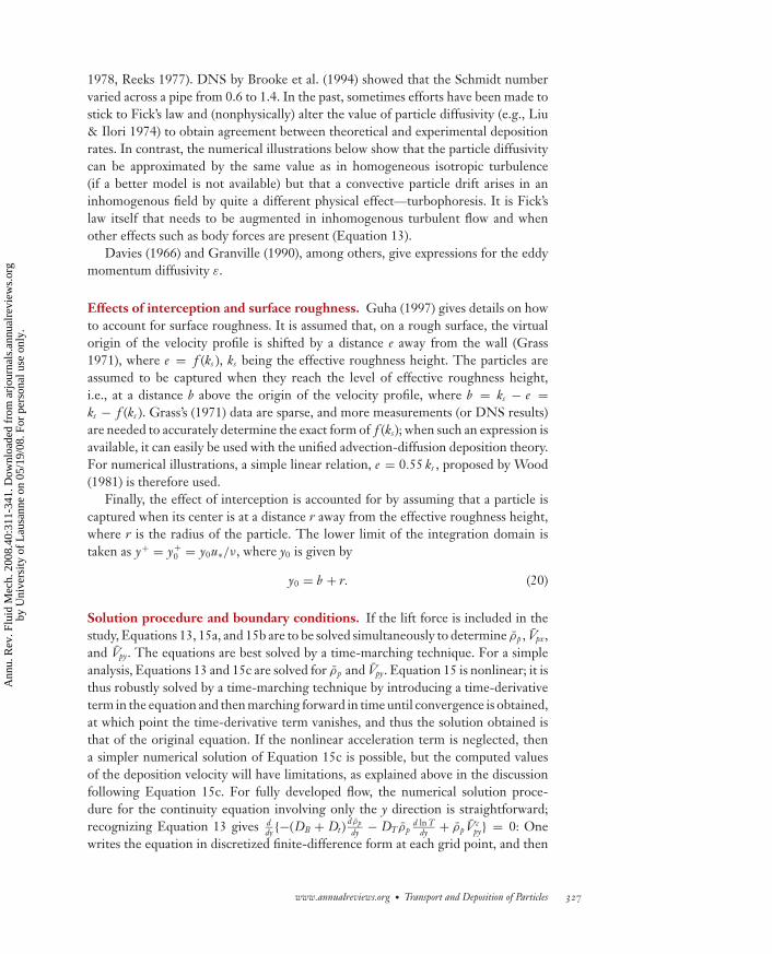
Figure 2Computed deposition rate versus relaxation time (effects of pure diffusion, pure inertia, andinterception): (red line) solution of Equation 13 retaining all terms; (orange line) pure diffusion,solution of Fick’s law (Equation 2) with lower boundary at wall (y+
0 = 0); (dark blue dashed line)pure diffusion, solution of Fick’s law (Equation 2) with interception (y+
0 = r+); and (light blueline) pure inertial deposition, solution of Equation 13 retaining only the third term on theright-hand side (i.e., the convective flux term alone). Blue dots denote experiments by Liu &Agarwal (1974). For all computed curves, k+
s = 0, �T = 0, and ξ = 0.
can be modeled without rebound); the pipe Reynolds number (ReD) was 10,000;and ρ0
p/ρ f = 770. By combining u∗ calculated from Blasius’s formula, Guha (1997)has shown that (DB/ν)2/3τ+1/3 = f (ReD, D, ρ0
p/ρ, fluid properties) = ψ . Thus fordifferent values of ψ , different curves of V+
dep versus τ+ are obtained.Figure 2 shows the relative importance of pure diffusion and pure inertial effects
in the equation for mass flux (Equation 13). To isolate the effects of fluid turbulence,the flow considered is isothermal (no thermal diffusion), and all body forces (suchas electrical forces) are absent. The pure diffusion case is calculated by assumingthat the turbulence is homogeneous. The source term on the right-hand side ofEquation 15c is zero; consequently, the convective velocity, V̄c
py, is zero. Under thesecircumstances, Equation 13 becomes identical to Equation 2—Fick’s law of diffusion.The deposition velocity monotonically decreases with increasing relaxation time.This case was calculated by taking the lower boundary at y+ = 0. The behaviorof the deposition velocity, however, changes if one includes the effects of interception.The lower boundary is now given by Equation 20. As the lower boundary is shifted,the effective resistance against mass transfer decreases. For large relaxation times,this effect can more than offset the effect of the lower Brownian diffusion coefficient,DB. For large relaxation times, the calculated deposition velocity therefore increases
www.annualreviews.org • Transport and Deposition of Particles 329
Ann
u. R
ev. F
luid
Mec
h. 2
008.
40:3
11-3
41. D
ownl
oade
d fr
om a
rjou
rnal
s.an
nual
revi
ews.
org
by U
nive
rsity
of
Lau
sann
e on
05/
19/0
8. F
or p
erso
nal u
se o
nly.
ANRV332-FL40-14 ARI 10 November 2007 16:27
substantially with increasing relaxation time owing to interception, even when theconvective velocity, V̄c
py, is neglected. (The interception effect shown in Figure 2 isthe minimum because it is shown for ks = 0, i.e., b = 0 in Equation 20.)
For calculating pure inertial effects, only the third term on the right-hand sideof Equation 13 is retained. Figure 2 shows that the convective velocity goes to zerofor very small particles. Its effect on the deposition velocity has become comparableto that of pure diffusion around τ+ ∼ 0.2. It then rises steeply by several orders ofmagnitude as τ+ increases. The total deposition is calculated by retaining all terms inEquation 13. It merges with the pure diffusion case for very small particles and withthe pure inertial case for large particles. One can clearly see the relative importanceof diffusion, inertia, and interception in Figure 2.
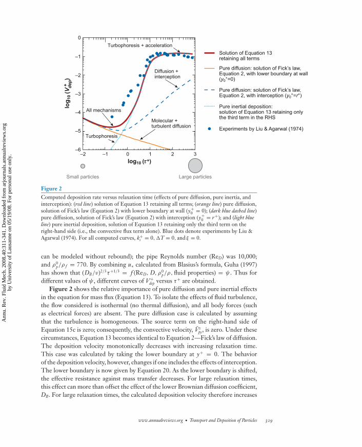
Figure 3 shows the variation in deposition velocity with relaxation time for fourdifferent roughness parameters. The calculations show that the presence of a smallamount of surface roughness even in the hydraulically smooth regime significantlyenhances deposition, especially that of small particles. Given that the depositionvelocity varies by more than four orders of magnitude in the range of investigation,it is remarkable that a simple, universal equation (Equation 13) agrees so well withmeasurements.
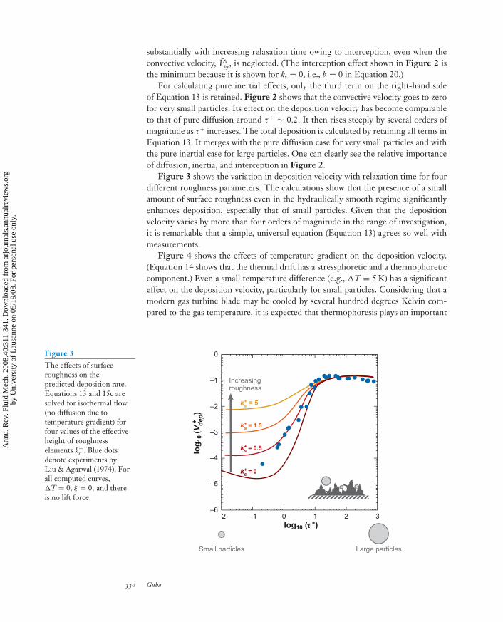
Figure 4 shows the effects of temperature gradient on the deposition velocity.(Equation 14 shows that the thermal drift has a stressphoretic and a thermophoreticcomponent.) Even a small temperature difference (e.g., �T = 5 K) has a significanteffect on the deposition velocity, particularly for small particles. Considering that amodern gas turbine blade may be cooled by several hundred degrees Kelvin com-pared to the gas temperature, it is expected that thermophoresis plays an important
ks+ = 0
ks+ = 0.5
ks+ = 1.5
ks+ = 5
log10 (ττ+)
Small particles Large particles
–2 –1 0 1 2 3–6
–5
–4
–3
–2
–1
0
Increasingroughness
log
10 (V
dep
)+
Figure 3The effects of surfaceroughness on thepredicted deposition rate.Equations 13 and 15c aresolved for isothermal flow(no diffusion due totemperature gradient) forfour values of the effectiveheight of roughnesselements k+
s . Blue dotsdenote experiments byLiu & Agarwal (1974). Forall computed curves,�T = 0, ξ = 0, and thereis no lift force.
330 Guha
Ann
u. R
ev. F
luid
Mec
h. 2
008.
40:3
11-3
41. D
ownl
oade
d fr
om a
rjou
rnal
s.an
nual
revi
ews.
org
by U
nive
rsity
of
Lau
sann
e on
05/
19/0
8. F
or p
erso
nal u
se o
nly.
ANRV332-FL40-14 ARI 10 November 2007 16:27
Tf
Increasingtemperaturegradient
T = 0
T = 5 K
T = 20 K
T = 50 K
log10 (τ+)
Small particles Large particles
–2 –1 0 1 2 3–6
–5
–4
–3
–2
–1
0
log
10 (V
dep
)+
Figure 4Effects of thermal diffusionon the predicted depositionrate. Equations 13 and 15care solved for four values of�T, where �T is thetemperature differencebetween the upperboundary of the calculationdomain (y+ = 200) and thepipe wall (the wall iscooled). Blue dots denoteexperiments by Liu &Agarwal (1974). For allcomputed curves,k+
s = 0, ξ = 0, and there isno lift force.
role there. For 1 < τ+ < 10, there is an interaction between thermophoresis andturbophoresis.
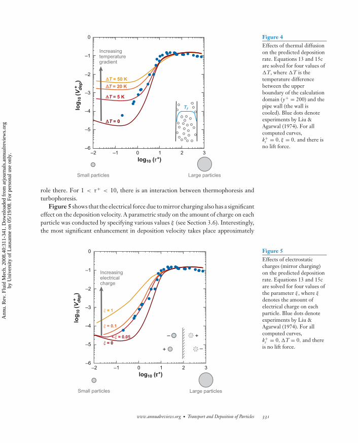
Figure 5 shows that the electrical force due to mirror charging also has a significanteffect on the deposition velocity. A parametric study on the amount of charge on eachparticle was conducted by specifying various values ξ (see Section 3.6). Interestingly,the most significant enhancement in deposition velocity takes place approximately
+
+–
–
Increasingelectrical charge
ξ = 0
ξ = 1
ξ = 0.05
ξ = 0.1
Small particles Large particles
–2 –1 0 1 2 3–6
–5
–4
–3
–2
–1
0
log10 (ττ+)
log
10 (V
dep
)+
Figure 5Effects of electrostaticcharges (mirror charging)on the predicted depositionrate. Equations 13 and 15care solved for four values ofthe parameter ξ , where ξ
denotes the amount ofelectrical charge on eachparticle. Blue dots denoteexperiments by Liu &Agarwal (1974). For allcomputed curves,k+
s = 0, �T = 0, and thereis no lift force.
www.annualreviews.org • Transport and Deposition of Particles 331
Ann
u. R
ev. F
luid
Mec
h. 2
008.
40:3
11-3
41. D
ownl
oade
d fr
om a
rjou
rnal
s.an
nual
revi
ews.
org
by U
nive
rsity
of
Lau
sann
e on
05/
19/0
8. F
or p
erso
nal u
se o
nly.
ANRV332-FL40-14 ARI 10 November 2007 16:27
around τ+ ∼ 0.3, at which the unassisted deposition curve begins to rise in Figure 2.Of course, the effects of the electrostatic forces are more prominent in the presenceof an external electric field.
The particle transport given by Equation 13 has a diffusive and a convectivepart. The particles are transported by these two mechanisms. (The old free flightis effectively calculated by the present model of turbophoresis.) Very small particlescomplete the last part of their journey to the wall mainly by Brownian diffusion,and very large particles reach the wall mainly by the convective velocity imparted byturbophoresis. For intermediate-sized particles, a combination of both mechanismsis responsible.
In the region close to the wall (e.g., y+ < 20), ∂J/∂y = 0 for fully developedflow; the total particle flux (convective plus diffusive) remains constant (i.e., whateverparticle flux enters into this region must reach the wall surface to satisfy continuityand to attain a steady state). Large particles may acquire sufficient V̄c
py to enable themto coast to the surface—in this case, ρ̄p would remain approximately constant closeto the wall. The convective velocity may not be sufficient for small particles to coastall the way to the surface; to keep the total particle flux constant to satisfy continuity,the convective flux in this case may need to be supplemented by a large diffusive flux,which is achieved by the appropriate development of a particle density profile close tothe wall. If the predicted value of V̄c
py close to wall is inaccurate or the wall boundarycondition for ρ̄p is improper, then to keep J invariant close to the wall, the predictedconcentration profile close to the wall would not be accurate.
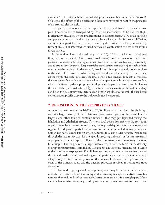
7. DEPOSITION IN THE RESPIRATORY TRACT
An adult human breathes in 10,000 to 20,000 liters of air per day. The air bringswith it a large quantity of particulate matter—micro-organisms, dusts, smokes, al-lergens, and other toxic or nontoxic aerosols—that may get deposited during theinhalation and exhalation process. The term total deposition refers to the collectionof particles in the whole respiratory tract, and regional deposition is that in a specifiedregion. The deposited particles may cause various effects, including many diseases.Sometimes particles of a known amount and size may also be deliberately introducedthrough the respiratory tract for therapeutic use (drug delivery), or for measurementsof prophylactic and therapeutic effects of inhaled substances and pulmonary function,for example. The lung has a very large surface area; thus it is suitable for the deliveryof drugs for both topical (minimizing side effects) and systemic (utilizing rapid accessto the blood stream) purposes. For all these reasons, experimental determination andtheoretical prediction of total and regional depositions are necessary. Consequentlya large body of literature has grown on this subject. In this section, I present a syn-opsis of the principal ideas and the physical processes involved in respiratory tractdeposition.
The flow in the upper part of the respiratory tract may be turbulent, whereas thatin the lower tract is laminar. For the types of bifurcating airways, the critical Reynoldsnumber above which flow becomes turbulent is lower than it is in a straight pipe. If thevolume flow rate increases (e.g., during exercise), turbulent flow persists lower down
332 Guha
Ann
u. R
ev. F
luid
Mec
h. 2
008.
40:3
11-3
41. D
ownl
oade
d fr
om a
rjou
rnal
s.an
nual
revi
ews.
org
by U
nive
rsity
of
Lau
sann
e on
05/
19/0
8. F
or p
erso
nal u
se o
nly.

ANRV332-FL40-14 ARI 10 November 2007 16:27
the tract than that during normal breathing. Turbulent flow increases deposition. Ingeneral, inertial impaction is significant in upper airways in which velocities are high;gravitational settling and Brownian diffusion are significant in lower airways in whichresidence times are longer. Typically, only a small proportion of the residual air in thealveolar region is actively replaced, leaving molecular diffusion to achieve a secondstage of ventilation of the relatively stagnant residual air deep in the lung.
The deposition pattern of inhaled particles is strongly determined by the sizeof particles. The size range of natural and manmade particles can be large: For ex-ample, occupational dusts may be 0.001–1000 μm, pollen particles are 20–60 μm,consumer aerosol products are 2–6 μm, most cigarette smoke particles are 0.2–0.6 μm, and viruses and proteins may be in the range 0.001–0.05 μm. Part of thepreviously deposited particles may be removed by various clearance mechanisms,such as solubilization and absorption, coughing, sneezing, mucociliary transport, andalveolar clearance mechanisms involving pulmonary macrophages and other mecha-nisms (Brain & Valberg 1979). For a simple description, Heyder et al. (1986) presentsdeposition data in three regions: extrathoracic (nasal plus laryngeal), tracheobronchial(upper plus lower), and alveolar.
Deposition depends on the characteristics of the particles (size, shape, density,charge), morphology of the respiratory tract, and the breathing pattern (which de-termines the volumetric flow rate and the mean residence time of a particle). Heyderet al. (1986) and Stahlhofen (1980), among others, have given detailed experimentaldata. Figure 6 shows a typical plot of fractional deposition in the three regions as afunction of particle diameter (of unit density 1 g cm−3); the main interest here is toexplain the qualitative physics.
0.0
0.2
0.4
0.6
0.8
1
0.001
Nasal
Laryngeal
Bronchial
Alveolar
Total
B
A
C
Particle diameter (µm)
Fra
ctio
nal
dep
osi
tio
n
0.01 0.1 1 10 100
Figure 6A typical regional deposition behavior in the human respiratory tract (as fractions of the totalinhaled quantity). For particle sizes approximately less than 0.3 μm, the total deposition curveis almost superposed with the alveolar deposition curve. The alveolar deposition curve isdivided into three segments A, B, and C to provide physical explanations regarding suchvariations. Data taken from Heyder et al. 1986.
www.annualreviews.org • Transport and Deposition of Particles 333
Ann
u. R
ev. F
luid
Mec
h. 2
008.
40:3
11-3
41. D
ownl
oade
d fr
om a
rjou
rnal
s.an
nual
revi
ews.
org
by U
nive
rsity
of
Lau
sann
e on
05/
19/0
8. F
or p
erso
nal u
se o
nly.
ANRV332-FL40-14 ARI 10 November 2007 16:27
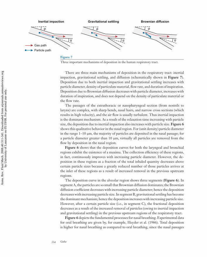
Inertial impaction Gravitational settling Brownian diffusion
Gas path
Particle path
φ
θ
φ
θ
φ
θ
Figure 7Three important mechanisms of deposition in the human respiratory tract.
There are three main mechanisms of deposition in the respiratory tract: inertialimpaction, gravitational settling, and diffusion (schematically shown in Figure 7).Deposition due to both inertial impaction and gravitational settling increases withparticle diameter, density of particulate material, flow rate, and duration of inspiration.Deposition due to Brownian diffusion decreases with particle diameter, increases withduration of inspiration, and does not depend on the density of particulate material orthe flow rate.
The passages of the extrathoracic or nasopharyngeal section (from nostrils tolarynx) are complex, with sharp bends, nasal hairs, and narrow cross sections (whichresults in high velocity), and the air flow is usually turbulent. Thus inertial impactionis the dominant mechanism. As a result of the relaxation time increasing with particlesize, the deposition due to inertial impaction also increases with particle size. Figure 6shows this qualitative behavior in the nasal region. For (unit density) particle diameterin the range 1–10 μm, the majority of particles are deposited in the nasal passage; fora particle diameter greater than 10 μm, virtually all particles are removed from theflow by deposition in the nasal region.
Figure 6 shows that the deposition curves for both the laryngeal and bronchialregions exhibit the existence of a maxima. The collection efficiency of these regions,in fact, continuously improves with increasing particle diameter. However, the de-position in these regions as a fraction of the total inhaled quantity decreases abovecertain particle sizes because a greatly reduced number of those particles arrives atthe inlet of these regions as a result of increased removal in the previous upstreamregions.
The deposition curve in the alveolar region shows three segments (Figure 6). Insegment A, the particles are so small that Brownian diffusion dominates; the Browniandiffusion coefficient decreases with increasing particle diameter; hence the depositiondecreases with increasing particle size. In segment B, gravitational settling has becomethe dominant mechanism; hence the deposition increases with increasing particle size.However, after a certain particle size (i.e., in segment C), the fractional depositiondecreases as a result of the increased removal of particles (owing to inertial impactionand gravitational settling) in the previous upstream regions of the respiratory tract.
Figure 6 depicts the fundamental processes for nasal breathing. Experimental datafor oral breathing are given by, for example, Heyder et al. (1986). Total depositionis higher for nasal breathing as compared to oral breathing, since the nasal passages
334 Guha
Ann
u. R
ev. F
luid
Mec
h. 2
008.
40:3
11-3
41. D
ownl
oade
d fr
om a
rjou
rnal
s.an
nual
revi
ews.
org
by U
nive
rsity
of
Lau
sann
e on
05/
19/0
8. F
or p
erso
nal u
se o
nly.
ANRV332-FL40-14 ARI 10 November 2007 16:27
are very effective collectors, particularly of large particles. However, the laryngeal,bronchial, and alveolar depositions are lower for nasal breathing.
Theories (e.g., Beeckmans 1965, Landahl 1963, Taulbee & Yu 1975) and semiem-pirical methods (e.g., Heyder et al. 1986, Int. Comm. Respir. Prot. 1994) have beendeveloped for the prediction of deposition in the respiratory tract. In recent years theapplication of CFD has opened up the possibility of achieving theoretical solutionsfor realistic, complex flow passages. Mostly, commercially available CFD softwarepackages have been used for the numerical simulation of the air flow field in the na-sopharyngeal or tracheobronchial tree. Particle deposition is then calculated mostlyby nonstochastic Lagrangian particle tracking (thus excluding any effect of fluid tur-bulence on particle motion) and occasionally by Eulerian modeling (but excludingturbophoresis). It will be interesting to study any effects of turbophoresis on the depo-sition in the upper airways. There is no doubt that computational studies of depositionin the respiratory tract will grow vigorously in the future. Once validated by experi-ments, the CFD tools have the potential to significantly enhance our understandingfor cases in which direct measurements would be difficult.
8. DEPOSITION IN GAS AND STEAM TURBINES
Both gas and steam turbine blades experience the high-speed flow of a gas or a vaporthrough highly curved, complex three-dimensional flow passages. Any suspendedsolid particles or liquid droplets therefore can move and get deposited by inertialimpaction (owing to streamline curvature) and by molecular and turbulent transportprocesses as explained above. In cooled gas turbines, in which the blade may be 300–400 K cooler than the gas, the thermal gradient also strongly influences the motion ofparticles [in the appropriate size range (Figure 4)]. The flow through turbine bladestherefore provides a good opportunity to test theoretical predictions. The flow fieldin the primary gas (or vapor) is determined by Eulerian flow solvers (e.g., Denton& Dawes 1999, Mei & Guha 2005); therefore, it is most profitable to integrate theunified Eulerian advection-diffusion model of deposition explained in Section 5.2with any available single-phase flow solver. The particle equations given by Guha(1997) can be used for developing boundary layers.
In low-pressure steam turbines, droplets form owing to homogeneous nucleationand then grow rapidly (Guha 1995, 1998b; Guha & Young 1994; Gyarmathy 1962).Experiments show that the water in turbines exists in two quite different forms.Usually more than 90% of the mass is concentrated in the fog, which consists of avery large number of very fine droplets (diameter 0.05–2.0 μm). The rest is in the formof coarse droplets that are much larger (diameter 20–200 μm). Coarse water is formedas a small proportion of the fog (typically 2%–4% per blade row) is deposited on theblade surface (Crane 1973, Parker & Ryley 1969/1970, Young & Yau 1988). Thedeposited water is drawn toward the trailing edge by the steam flow (or centrifugedtoward the casing on moving blades), at which it is re-entrained in the form of largedroplets. Impingement of the large droplets causes blade erosion.
Menguturk & Sverdrup (1982) have computed deposition on gas turbine blades.Deposition causes erosion and corrosion. The turbines, situated downstream of the
www.annualreviews.org • Transport and Deposition of Particles 335
Ann
u. R
ev. F
luid
Mec
h. 2
008.
40:3
11-3
41. D
ownl
oade
d fr
om a
rjou
rnal
s.an
nual
revi
ews.
org
by U
nive
rsity
of
Lau
sann
e on
05/
19/0
8. F
or p
erso
nal u
se o
nly.
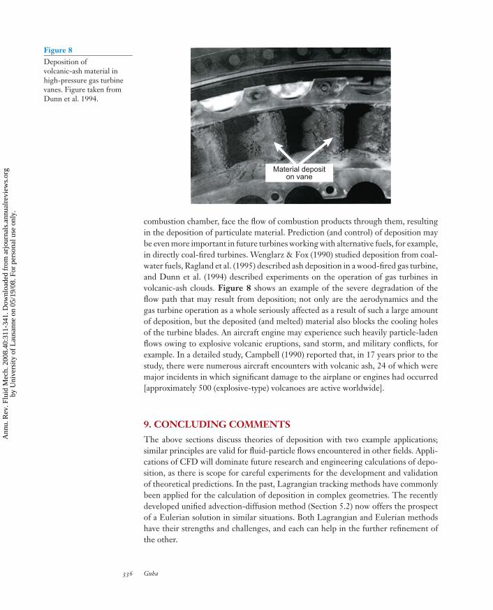
ANRV332-FL40-14 ARI 10 November 2007 16:27
Material depositon vane
Figure 8Deposition ofvolcanic-ash material inhigh-pressure gas turbinevanes. Figure taken fromDunn et al. 1994.
combustion chamber, face the flow of combustion products through them, resultingin the deposition of particulate material. Prediction (and control) of deposition maybe even more important in future turbines working with alternative fuels, for example,in directly coal-fired turbines. Wenglarz & Fox (1990) studied deposition from coal-water fuels, Ragland et al. (1995) described ash deposition in a wood-fired gas turbine,and Dunn et al. (1994) described experiments on the operation of gas turbines involcanic-ash clouds. Figure 8 shows an example of the severe degradation of theflow path that may result from deposition; not only are the aerodynamics and thegas turbine operation as a whole seriously affected as a result of such a large amountof deposition, but the deposited (and melted) material also blocks the cooling holesof the turbine blades. An aircraft engine may experience such heavily particle-ladenflows owing to explosive volcanic eruptions, sand storm, and military conflicts, forexample. In a detailed study, Campbell (1990) reported that, in 17 years prior to thestudy, there were numerous aircraft encounters with volcanic ash, 24 of which weremajor incidents in which significant damage to the airplane or engines had occurred[approximately 500 (explosive-type) volcanoes are active worldwide].
9. CONCLUDING COMMENTS
The above sections discuss theories of deposition with two example applications;similar principles are valid for fluid-particle flows encountered in other fields. Appli-cations of CFD will dominate future research and engineering calculations of depo-sition, as there is scope for careful experiments for the development and validationof theoretical predictions. In the past, Lagrangian tracking methods have commonlybeen applied for the calculation of deposition in complex geometries. The recentlydeveloped unified advection-diffusion method (Section 5.2) now offers the prospectof a Eulerian solution in similar situations. Both Lagrangian and Eulerian methodshave their strengths and challenges, and each can help in the further refinement ofthe other.
336 Guha
Ann
u. R
ev. F
luid
Mec
h. 2
008.
40:3
11-3
41. D
ownl
oade
d fr
om a
rjou
rnal
s.an
nual
revi
ews.
org
by U
nive
rsity
of
Lau
sann
e on
05/
19/0
8. F
or p
erso
nal u
se o
nly.

ANRV332-FL40-14 ARI 10 November 2007 16:27
DISCLOSURE STATEMENT
The author is not aware of any biases that might be perceived as affecting the objec-tivity of this review.
ACKNOWLEDGEMENTS
I thank the Editors for asking me to contribute and the Annual Reviews productionstaff for sustaining excellence. I am grateful to my family members, friends, teach-ers, institutes, and researchers worldwide who have contributed to my existence andlearning.
LITERATURE CITED
Beal SK. 1970. Deposition of particles in turbulent flow on channel or pipe walls.Nucl. Sci. Eng. 40:1–11
Becker E. 1970. Relaxation effects in gas dynamics. Aeronaut. J. 74:736–48Beeckmans JM. 1965. Deposition of aerosols in respiratory tract. I. Mathemati-
cal analysis and comparison with experimental data. Can. J. Physiol. Pharmacol.43:157–72
Berlemont A, Desjonqueres P, Gouesbet G. 1990. Particle Lagrangian simulation inturbulent flows. Int. J. Multiph. Flow 16:19–34
Binder JL, Hanratty TJ. 1991. A diffusion model for droplet deposition in gas/liquidannular flow. Int. J. Multiph. Flow 17:1–11
Borgas MS, Sawford BL. 1996. Molecular diffusion and viscous effects in grid turbu-lence. J. Fluid Mech. 324:25–54
Brain JD, Valberg PA. 1979. Deposition of aerosol in the respiratory tract. Am. Rev.Respir. Dis. 120:1325–73
Bremhorst K, Walker TB. 1973. Spectral measurements of turbulent momentumtransfer in fully developed pipe flow. J. Fluid Mech. 61:173–86
Brooke JW, Hanratty TJ, McLaughlin JB. 1994. Free-flight mixing and depositionof aerosols. Phys. Fluids 6:3404–15
Campbell EE. 1990. Volcanic ash. Proc. 747 Flight Oper. Symp. Seattle, WA, Oct. 9–11,pp. 2.3.1–34. Seattle: Boeing Commer. Aircr. Co.
Caporaloni M, Tampieri F, Trombetti F, Vittori O. 1975. Transport of particles innonisotropic air turbulence. J. Atmos. Sci. 32:565–68
Chapman DR, Kuhn GD. 1986. The limiting behaviour of turbulence near a wall.J. Fluid Mech. 170:265–92
Cleaver JW, Yates B. 1975. A sub-layer model for the deposition of particles from aturbulent flow. Chem. Eng. Sci. 30:983–92
Clift R, Grace JR, Weber ME. 1978. Bubbles, Drops and Particles. New York: AcademicCrane RI. 1973. Deposition of fog drops on low pressure steam turbine blades. Int.
J. Mech. Sci. 15:613–31Crowe CT. 1982. Review. Numerical models for dilute gas-particle flows. J. Fluids
Eng. 104:297–303
www.annualreviews.org • Transport and Deposition of Particles 337
Ann
u. R
ev. F
luid
Mec
h. 2
008.
40:3
11-3
41. D
ownl
oade
d fr
om a
rjou
rnal
s.an
nual
revi
ews.
org
by U
nive
rsity
of
Lau
sann
e on
05/
19/0
8. F
or p
erso
nal u
se o
nly.
ANRV332-FL40-14 ARI 10 November 2007 16:27
Cunningham E. 1910. On the velocity of steady fall of spherical particles throughfluid medium. Proc. R. Soc. Lond. Ser. A 83:357–65
Davies CN. 1945. Definitive equations for the fluid resistance of spheres. Proc. Phys.Soc. Lond. 57:259–70
Davies CN, ed. 1966. Aerosol Science. London: AcademicDenton JD, Dawes WN. 1999. Computational fluid dynamics for turbomachinery
design. Proc. Inst. Mech. Eng. C 213:107–24Dunn MG, Baran AJ, Miatech J. 1994. Operation of gas turbine engines in volcanic
ash clouds. ASME Tech. Pap. 94-GT-170Durbin PA. 1980. A random flight model of inhomogeneous turbulent dispersion.
Phys. Fluids 23:2151–53Fan F, Ahmadi G. 1993. A sublayer model for turbulent deposition of particles in
vertical ducts with smooth and rough surfaces. J. Aerosol Sci. 24:45–64Fernandez De La Mora JF, Rosner DE. 1982. Effects of inertia on the diffusional
deposition of small particles to spheres and cylinders at low Reynolds numbers.J. Fluid Mech. 125:379–95
Fichman M, Gutfinger C, Pnueli D. 1988. A model for turbulent deposition ofaerosols. J. Aerosol Sci. 19:123–36
Finnicum DS, Hanratty TJ. 1985. Turbulent normal velocity fluctuations close to awall. Phys. Fluids 28:1654–58
Friedlander SK, Johnstone HF. 1957. Deposition of suspended particles from turbu-lent gas streams. Ind. Eng. Chem. 49:1151–56
Gosman AD, Ioannides E. 1983. Aspects of computer simulation of liquid-fueledcombustors. J. Energy 7:482–90
Graham DI, James PW. 1996. Turbulent dispersion of particles using eddy interactionmodels. Int. J. Multiph. Flow 22:157–75
Granville PS. 1990. A near-wall eddy viscosity formula for turbulent boundary lay-ers in pressure gradients suitable for momentum, heat, or mass transfer. Trans.ASME J. Fluids Eng. 112:240–43
Grass AJ. 1971. Structural features of turbulent flow over smooth and rough bound-aries. J. Fluid Mech. 50:233–55
Guha A. 1994. A unified theory of aerodynamic and condensation shock waves invapour-droplet flows with or without a carrier gas. Phys. Fluids 6:1893–913
Guha A. 1995. Two-phase flows with phase transition: nucleation, droplet growthand condensation in pure steam flows; fluid dynamics with interphase trans-port of mass, momentum and energy in pure vapour-droplet mixtures; applica-tion of the non-equilibrium theory to steam turbines. In Two-Phase Flows withPhase Transition, pp. 1–110. Von Karman Inst. Lect. Ser. 1995–06. Belgium:von Karman Inst. Fluid Dyn.
Guha A. 1997. A unified Eulerian theory of turbulent deposition to smooth and roughsurfaces. J. Aerosol Sci. 28:1517–37
Guha A. 1998a. A unified theory for the interpretation of total pressure and temper-ature in two-phase flows at subsonic and supersonic speeds. Proc. R. Soc. Ser. A454:671–95
Guha A. 1998b. Computation, analysis and theory of two-phase flows. Aeronaut. J.102:71–82
338 Guha
Ann
u. R
ev. F
luid
Mec
h. 2
008.
40:3
11-3
41. D
ownl
oade
d fr
om a
rjou
rnal
s.an
nual
revi
ews.
org
by U
nive
rsity
of
Lau
sann
e on
05/
19/0
8. F
or p
erso
nal u
se o
nly.
ANRV332-FL40-14 ARI 10 November 2007 16:27
Guha A. 2007. Shock waves in fluids with interphase transport of mass, momentumand energy (vapour-droplet mixtures and solid-particle-laden gases). In ShockWaves Science and Technology Reference Library, Vol. 1, Multiphase Flows, ed. MEHvan Dongen, pp. 135–86. Berlin: Springer
Guha A, Young JB. 1991. Time-marching prediction of unsteady condensation phe-nomena due to supercritical heat addition. In Turbomachinery: Latest Developmentsin a Changing Scene, pp. 167–77. London: Inst. Mech. Eng.
Guha A, Young JB. 1994. The effect of flow unsteadiness on the homogeneous nucle-ation of water droplets in steam turbines. Philos. Trans. R. Soc. Lond. A 349:445–72
Gyarmathy G. 1962. Bases of a theory for wet steam turbines. Bull. 6, Inst. Therm.Turbomach., Fed. Tech. Univ., Zurich (CEGB translation 3017)
Hesketh HE. 1977. Fine Particles in Gaseous Media. Ann Arbor, MI: Ann Arbor Sci.Heyder J, Gebhart J, Rudolf G, Schiller CF, Stahlhofen W. 1986. Deposition of
particles in the human respiratory tract in the size range 0.005–15 μm. J. AerosolSci. 17:811–25
Hinds WC. 1999. Aerosol Technology: Properties, Behaviour and Measurement of AirborneParticles. New York: Wiley
Hutchinson P, Hewitt GF, Dukler AE. 1971. Deposition of liquid or solid dispersionsfrom turbulent gas streams: a stochastic model. Chem. Eng. Sci. 26:419–39
Int. Comm. Respir. Prot. 1994. Human Respiratory Tract Model for Radiological Protec-tion. Int. Comm. Respir. Prot. Publ. 66. Oxford: Pergamon
Johansen ST. 1991. The deposition of particles on vertical walls. Int. J. Multiph. Flow17:355–76
Kallio GA, Reeks MW. 1989. A numerical simulation of particle deposition in tur-bulent boundary layers. Int. J. Multiph. Flow 15:433–46
Kay JM, Nedderman RM. 1988. Fluid Mechanics and Transfer Processes. Cambridge,UK: Cambridge Univ. Press
Kim J, Moin P, Moser R. 1987. Turbulence statistics in fully developed channel flow.J. Fluid Mech. 177:136–66
Kreplin HP, Eckelmann H. 1979. Behaviour of the three fluctuating velocity com-ponents in the wall region of a turbulent channel flow. Phys. Fluids 22:1233–39
Landahl HD. 1963. Particle removal by the respiratory system. Bull. Math. Biophys.25:29–39
Laufer J. 1954. The structure of turbulence in fully developed pipe flow. NACA Tech.Rep. 1174
Liu BYH, Agarwal JK. 1974. Experimental observation of aerosol deposition in tur-bulent flow. J. Aerosol Sci. 5:145–55
Liu BYH, Ilori TY. 1974. Aerosol deposition in turbulent pipe flow. Environ. Sci.Technol. 8:351–56
Luhar AK, Britter RE. 1989. A random walk model for dispersion in inhomogeneousturbulence in a convective boundary layer. Atmos. Environ. 23:1911–24
Marchioli C, Soldati A. 2002. Mechanisms for particle transfer and segregation inturbulent boundary layers. J. Fluid Mech. 468:283–315
Maxey MR, Riley JJ. 1983. Equation of motion for a small rigid sphere in a nonuni-form flow. Phys. Fluids 26:883–89
www.annualreviews.org • Transport and Deposition of Particles 339
Ann
u. R
ev. F
luid
Mec
h. 2
008.
40:3
11-3
41. D
ownl
oade
d fr
om a
rjou
rnal
s.an
nual
revi
ews.
org
by U
nive
rsity
of
Lau
sann
e on
05/
19/0
8. F
or p
erso
nal u
se o
nly.
ANRV332-FL40-14 ARI 10 November 2007 16:27
McCoy DD, Hanratty TJ. 1977. Rate of deposition of droplets in annular two-phaseflow. Int. J. Multiph. Flow 3:319–31
Mei Y, Guha A. 2005. Implicit numerical simulation of transonic flow through tur-bine cascades on unstructured grids. Proc. Inst. Mech. Eng. A J. Power Energy219(A1):35–47
Menguturk M, Sverdrup EF. 1982. A theory for fine particle deposition in two-dimensional boundary layer flows and application to gas turbines. J. Eng. Power104:69–76
Monin AS, Yaglom AM. 1975. Statistical Fluid Mechanics: Mechanics of Turbulence,Vol. 2. Cambridge, MA: MIT Press
Morsi SA, Alexander AJ. 1972. An investigation of particle trajectories in two-phaseflow systems. J. Fluid Mech. 55:193–208
Nadler B, Hollerbach U, Eisenberg RS. 2003. Dielectric boundary force and itscrucial role in gramicidin. Phys. Rev. E 68:021905
Ounis H, Ahmadi G, McLaughlin JB. 1993. Brownian particle deposition in a directlysimulated turbulent channel flow. Phys. Fluids 5:1427–32
Papavergos PG, Hedley AB. 1984. Particle deposition behaviour from turbulentflows. Chem. Eng. Res. Des. 62:275–95
Parker GJ, Ryley DJ. 1969/1970. Equipment and techniques for studying the deposi-tion of submicron particles on turbine blades. Proc. Inst. Mech. Eng. 184(3C):43–51
Pismen LM, Nir A. 1978. On the motion of suspended particles in stationary homo-geneous turbulence. J. Fluid Mech. 84:193–206
Ragland KW, Misra MK, Aerts DJ, Palmer CA. 1995. Ash deposition in a wood-firedgas turbine. J. Eng. Gas Turbines Power 117:509–12
Ramshaw JD. 1979. Brownian motion in a flowing fluid. Phys. Fluids 22:1595–601Reeks MW. 1977. On the dispersion of small particles suspended in an isotropic
turbulent fluid. J. Fluid Mech. 83:529–46Reeks MW. 1983. The transport of discrete particles in inhomogeneous turbulence.
J. Aerosol Sci. 14:729–39Reeks MW. 1991. On a kinetic equation for the transport of particles in turbulent
flows. Phys. Fluids A 3:446–56Reeks MW. 1992. On the continuum equations for dispersed particles in nonuniform
flows. Phys. Fluids 4:1290–303Reeks MW, Skyrme G. 1976. The dependence of particle deposition velocity on
particle inertia in turbulent pipe flow. J. Aerosol Sci. 7:485–95Rizk MA, Elghobashi SE. 1985. The motion of a spherical particle suspended in a
turbulent flow near a plane wall. Phys. Fluids 28:806–17Saffman PG. 1965. The lift on a small sphere in a slow shear flow. J. Fluid Mech.
22:385–400Saffman PG. 1968. Corrigendum to “the lift on a small sphere in a slow shear flow.”
J. Fluid Mech. 31:624Sawford BL. 1982. Lagrangian Monte Carlo simulation of turbulent motion of a pair
of particles. Q. J. R. Meteorol. Soc. 108:207–13Shin M, Lee JW. 2001. Memory effect in the Eulerian particle deposition in a fully
developed turbulent channel flow. J. Aerosol Sci. 32:675–93
340 Guha
Ann
u. R
ev. F
luid
Mec
h. 2
008.
40:3
11-3
41. D
ownl
oade
d fr
om a
rjou
rnal
s.an
nual
revi
ews.
org
by U
nive
rsity
of
Lau
sann
e on
05/
19/0
8. F
or p
erso
nal u
se o
nly.

ANRV332-FL40-14 ARI 10 November 2007 16:27
Shuen JS, Chen LD, Faeth GM. 1983. Evaluation of a stochastic model of particledispersion in a turbulent round jet. Chem. Eng. J. 29:167–70
Simonin O, Deutsch E, Minier M. 1993. Eulerian prediction of the fluid-particlecorrelated motion in turbulent two-phase flows. Appl. Sci. Res. 51:275–83
Soo SL. 1990. Multiphase Fluid Dynamics. Beijing: ScienceStahlhofen W. 1980. Experimental determination of the regional deposition of
aerosol particles in the human respiratory tract. Am. Ind. Hyg. Assoc. J. 41:385–98Talbot L, Cheng RK, Schefer RW, Willis DR. 1980. Thermophoresis of particles in
a heated boundary layer. J. Fluid Mech. 101:737–58Taulbee DB, Yu CP. 1975. Theory of aerosol deposition in human respiratory tract.
J. Appl. Physiol. 38:77–85Thomson DJ. 1987. Criteria for the selection of stochastic models of particle trajec-
tories in turbulent flows. J. Fluid Mech. 180:529–56Vames JS, Hanratty TJ. 1988. Turbulent dispersion of droplets for air flow in a pipe.
Exp. Fluids 6:94–104Walklate PJ. 1987. A random-walk model for dispersion of heavy particles in turbulent
air flow. Bound. Layer Meteorol. 39:175–90Wang LP, Stock DE. 1992. Stochastic trajectory models for turbulent diffusion:
Monte Carlo process versus Markov chains. Atmos. Environ. 26:A1599–607Wang Q, Squires KD. 1996. Large eddy simulation of particle-laden turbulent chan-
nel flow. Phys. Fluids 8:1207–23Wells AC, Chamberlain AC. 1967. Transport of small particles to vertical surfaces.
Br. J. Appl. Phys. 18:1793–99Wenglarz RA, Fox RG. 1990. Physical aspects of deposition from coal-water fuels
under gas turbine conditions. J. Eng. Gas Turbines Power 112:9–14Wood NB. 1981. A simple method for the calculation of turbulent deposition to
smooth and rough surfaces. J. Aerosol Sci. 12:275–90Young J, Leeming A. 1997. A theory of particle deposition in turbulent pipe flow.
J. Fluid Mech. 340:129–59Young JB, Yau KK. 1988. The inertial deposition of fog droplets on steam turbine
blades. J. Turbomach. 110:155–62Zaichik LI. 1999. A statistical model of particle transport and heat transfer in turbulent
shear flows. Phys. Fluids 11:1521–34
www.annualreviews.org • Transport and Deposition of Particles 341
Ann
u. R
ev. F
luid
Mec
h. 2
008.
40:3
11-3
41. D
ownl
oade
d fr
om a
rjou
rnal
s.an
nual
revi
ews.
org
by U
nive
rsity
of
Lau
sann
e on
05/
19/0
8. F
or p
erso
nal u
se o
nly.
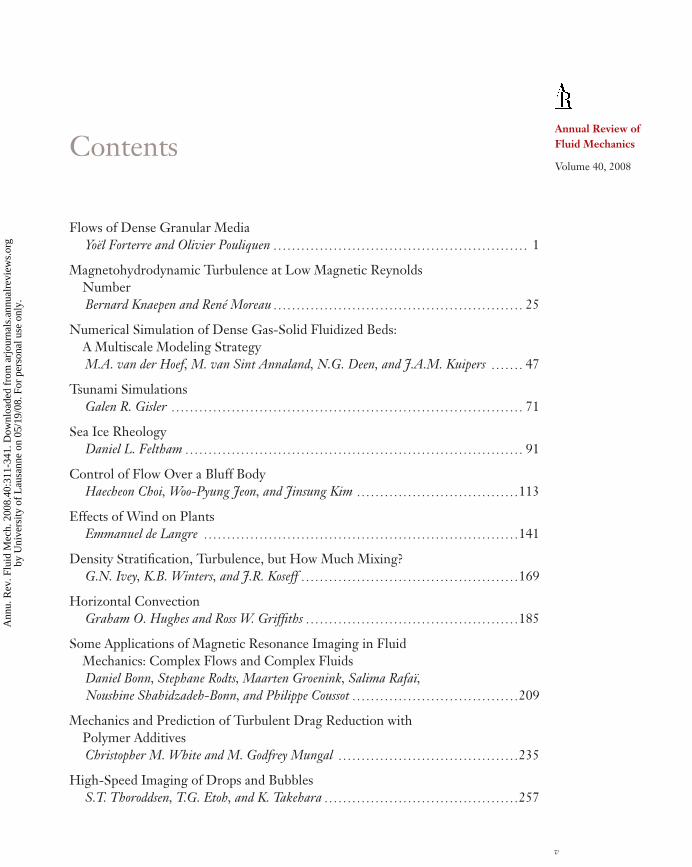
AR332-FM ARI 22 November 2007 21:57
Annual Review ofFluid Mechanics
Volume 40, 2008Contents
Flows of Dense Granular MediaYoël Forterre and Olivier Pouliquen � � � � � � � � � � � � � � � � � � � � � � � � � � � � � � � � � � � � � � � � � � � � � � � � � � � � � � � 1
Magnetohydrodynamic Turbulence at Low Magnetic ReynoldsNumberBernard Knaepen and René Moreau � � � � � � � � � � � � � � � � � � � � � � � � � � � � � � � � � � � � � � � � � � � � � � � � � � � � � � 25
Numerical Simulation of Dense Gas-Solid Fluidized Beds:A Multiscale Modeling StrategyM.A. van der Hoef, M. van Sint Annaland, N.G. Deen, and J.A.M. Kuipers � � � � � � � 47
Tsunami SimulationsGalen R. Gisler � � � � � � � � � � � � � � � � � � � � � � � � � � � � � � � � � � � � � � � � � � � � � � � � � � � � � � � � � � � � � � � � � � � � � � � � � � � � 71
Sea Ice RheologyDaniel L. Feltham � � � � � � � � � � � � � � � � � � � � � � � � � � � � � � � � � � � � � � � � � � � � � � � � � � � � � � � � � � � � � � � � � � � � � � � � � 91
Control of Flow Over a Bluff BodyHaecheon Choi, Woo-Pyung Jeon, and Jinsung Kim � � � � � � � � � � � � � � � � � � � � � � � � � � � � � � � � � � �113
Effects of Wind on PlantsEmmanuel de Langre � � � � � � � � � � � � � � � � � � � � � � � � � � � � � � � � � � � � � � � � � � � � � � � � � � � � � � � � � � � � � � � � � � � �141
Density Stratification, Turbulence, but How Much Mixing?G.N. Ivey, K.B. Winters, and J.R. Koseff � � � � � � � � � � � � � � � � � � � � � � � � � � � � � � � � � � � � � � � � � � � � � � �169
Horizontal ConvectionGraham O. Hughes and Ross W. Griffiths � � � � � � � � � � � � � � � � � � � � � � � � � � � � � � � � � � � � � � � � � � � � � �185
Some Applications of Magnetic Resonance Imaging in FluidMechanics: Complex Flows and Complex FluidsDaniel Bonn, Stephane Rodts, Maarten Groenink, Salima Rafaï,Noushine Shahidzadeh-Bonn, and Philippe Coussot � � � � � � � � � � � � � � � � � � � � � � � � � � � � � � � � � � � �209
Mechanics and Prediction of Turbulent Drag Reduction withPolymer AdditivesChristopher M. White and M. Godfrey Mungal � � � � � � � � � � � � � � � � � � � � � � � � � � � � � � � � � � � � � � �235
High-Speed Imaging of Drops and BubblesS.T. Thoroddsen, T.G. Etoh, and K. Takehara � � � � � � � � � � � � � � � � � � � � � � � � � � � � � � � � � � � � � � � � � �257
v
Ann
u. R
ev. F
luid
Mec
h. 2
008.
40:3
11-3
41. D
ownl
oade
d fr
om a
rjou
rnal
s.an
nual
revi
ews.
org
by U
nive
rsity
of
Lau
sann
e on
05/
19/0
8. F
or p
erso
nal u
se o
nly.
AR332-FM ARI 22 November 2007 21:57
Oceanic Rogue WavesKristian Dysthe, Harald E. Krogstad, and Peter Müller � � � � � � � � � � � � � � � � � � � � � � � � � � � � � � �287
Transport and Deposition of Particles in Turbulent and Laminar FlowAbhijit Guha � � � � � � � � � � � � � � � � � � � � � � � � � � � � � � � � � � � � � � � � � � � � � � � � � � � � � � � � � � � � � � � � � � � � � � � � � � � � � �311
Modeling Primary AtomizationMikhael Gorokhovski and Marcus Herrmann � � � � � � � � � � � � � � � � � � � � � � � � � � � � � � � � � � � � � � � � � �343
Blood Flow in End-to-Side AnastomosesFrancis Loth, Paul F. Fischer, and Hisham S. Bassiouny � � � � � � � � � � � � � � � � � � � � � � � � � � � � � � �367
Applications of Acoustics and Cavitation to Noninvasive Therapy andDrug DeliveryConstantin C. Coussios and Ronald A. Roy � � � � � � � � � � � � � � � � � � � � � � � � � � � � � � � � � � � � � � � � � � � � � �395
Indexes
Subject Index � � � � � � � � � � � � � � � � � � � � � � � � � � � � � � � � � � � � � � � � � � � � � � � � � � � � � � � � � � � � � � � � � � � � � � � � � � � � � � � �421
Cumulative Index of Contributing Authors, Volumes 1–40 � � � � � � � � � � � � � � � � � � � � � � � � � �431
Cumulative Index of Chapter Titles, Volumes 1–40 � � � � � � � � � � � � � � � � � � � � � � � � � � � � � � � � � �439
Errata
An online log of corrections to Annual Review of Fluid Mechanics articles may befound at http://fluid.annualreviews.org/errata.shtml
vi Contents
Ann
u. R
ev. F
luid
Mec
h. 2
008.
40:3
11-3
41. D
ownl
oade
d fr
om a
rjou
rnal
s.an
nual
revi
ews.
org
by U
nive
rsity
of
Lau
sann
e on
05/
19/0
8. F
or p
erso
nal u
se o
nly.