The University of Birmingham

Nature Inspired Techniques in Traffic

Management & Route Optimisation By Thomas Barker, Andrew Matthews & Nathan Collins

07/03/2011

Abstract: Traditional research into the problems associated with traffic management

have focussed on complex scientific models, such as fluid dynamics, to model and find

optimal traffic solutions. This report instead draws inspiration from nature to highlight

systems that can be computationally cheaper and manage traffic more efficiently than

conventional techniques. All three natural techniques presented; cellular automata,

evolutionary algorithms and ant algorithms, put forward an alternative to prevalent

centralised traffic control systems that are slow to react to or are blind to the current

traffic conditions.

Table of Contents

Nature Inspired Techniques in Traffic Management & Route Optimisation .........................................1

1 Introduction ....................................................................................................................................3

2 Cellular automata in traffic modelling and control.........................................................................4

2.1 Cellular automaton introduction ............................................................................................4

2.2 Traffic models using cellular automaton ................................................................................4

2.3 Traffic control using cellular automata...................................................................................6

2.3.1 Current traffic control methods......................................................................................6

2.3.2 Self organising traffic lights (SOTL) .................................................................................7

2.4 Cellular Automata in traffic summary.....................................................................................9

3 Introduction to Evolutionary Algorithms......................................................................................11

3.1 Salt Routing Optimisation .....................................................................................................11

3.2 Adaptive Traffic Control........................................................................................................12

3.3 Evolutionary Computation Applied to Urban Traffic Optimisation ......................................13

3.4 Decentralised Car Traffic Control Using Message Propagation............................................14

4 Ant Colony Optimisation...............................................................................................................17

4.1 Vehicle Routing Problems.....................................................................................................18

4.1.1 Representation and Evaluation.....................................................................................18

4.2 Time-dependant Travel Times ..............................................................................................19

4.3 Dynamic Traffic Routing........................................................................................................21

5 Conclusion.....................................................................................................................................24

6 References ....................................................................................................................................25

1 Introduction

Traffic is a nuisance that wastes time and costs money. It causes additional stress for the people

involved and often harms social relations. On top of this emissions are equivalent to some industrial

sectors, contributing to greenhouse gases, and the location of emissions are predominantly in

densely populated areas.

It is difficult to calculate estimates of the economical costs of traffic, but as they can take hours off

an employee’s potential working hours per week, burn vast quantities of fuel unnecessarily, and

cause delays to business deliveries, the costs are assumed to be large. In Copenhagen, it has been

estimated that the economic loss due to vehicle delays is 750 million Euros per year, and for the

whole of Germany the damage has been estimated as 100 billion dollars per year [Szklarski 2010].

But with an exploding global population, of which an unprecedented 50 % now live in urban areas,

the challenges to improve traffic flow are great. Particularly when western middle classes have

grown, bringing with them an increase in average number of cars per household and therefore total

vehicles on road networks designed for significantly smaller capacities. These trends are likely to be

seen in the fast growing Eastern economies of China and India, which have amongst them some of

the largest cities in the World, in Mumbai and Shanghai. Efficiently processing vehicles through a

road network, particularly in urban areas has therefore become an important economic, social and

technical challenge of the modern industrial World.

In nature we see many examples of systems that can cope with dynamic changing environments

very successfully. These examples range from small scale interactions on a cellular level to processes

that take a quarter of a million years. This report will focus on the nature inspired techniques of

cellular automata, evolutionary algorithms and ant algorithms.

2 Cellular automata in traffic modelling and control

2.1 Cellular automaton introduction

Understanding the flow of traffic has traditionally been considered a time consuming, complex,

multivariable system that requires detailed models to be developed to simulate the behaviour of

individual vehicles. However more recently a lot of work has been focussed on modelling traffic

behaviour using cellular automata models, which have the main advantage of being more efficient

and have a faster performance when simulated on a computer.

Cellular automata have largely been considered a curiosity or side project since early work by Von

Neumann was made famous through Conway’s “Game of life”. In this game, a discrete element

known as a cellular automaton interacts with its neighbours over discrete increments of time, based

on predefined simple, local rules of interaction. These rules often lead to more complex and

interesting global behaviour, and are furthermore influenced by the initial states of the cellular

automata located on a discrete lattice of cells. The global behaviour that emerges is difficult to

predict and many different rule sets have been devised.

Four main attributes need to be defined when building a cellular automata model; the physical

environment, the cell’s state, the cell’s neighbourhood and, of course, a local transition rule

[Quartieri et al, 2010]. The physical environment describes the structure of the lattice that consists

of these cellular automata i.e. is it a finite square lattice, or hexagonal, etc. Typically each cellular

automata will be of equal size, and the dimensionality of the lattice also needs to be defined. A 1D

string of cells would be considered an elementary cellular automaton (ECA). The cell’s state is

normally assigned a binary integer that corresponds to one of two states, like in the “Game of life”

where each cell can either be alive (1) or dead (0). In a 2D lattice neighbourhoods fall in two main

categories, the Moore neighbourhood which considers all of the surrounding eight cells and the Von

Neumann neighbourhood which considers the four cells directly north, south, east and west of a

particular cell. However in an ECA the neighbourhood could be considered simply the two cells

either side of a particular cell or multiple cells in either direction. Finally the local transition rule is

defined that determines whether each cell will change state or not based on its own state and the

states of the cells in its neighbourhood. The same rule must be applied to all the elements else the

system is called a hybrid cellular automaton. If there are no probabilistic interactions incorporated in

the automaton then it can further be called a deterministic model [Quartieri et al, 2010].

2.2 Traffic models using cellular automaton

In the classic model developed by Kai Nagel and Michael Schreckenburg (1992), only single lane

traffic is considered in an ECA lattice, based upon rules that coincide with Wolfram’s rule 184

[Boccara & Fuks, 1998]. Here each of the cells can either be empty or occupied by exactly one

vehicle and the length of each cell is normally defined as 7.5 m; the average length of a car plus

reasonable safety distance. Given a time increment of 1 second, this corresponds to a change in

velocity of 28 km/h or 17.4 miles/h for the Nagel and Schreckenburg model [Quartieri et al, 2010]

which is built for highway (motorway) driving, where these changes in speed are more likely. Each

vehicle in the model has a velocity between zero and Vmax (where Vmax may or may not correspond to

the speed limit), and during a time increment, four consecutive steps are executed to update each

individual velocity [Nagel & Schreckenburg, 1992]:

1. Acceleration – if the velocity v of a car is less than Vmax, and if the distance to the next car is

larger than v + 1, the speed is advanced by one i.e. v = v + 1.

2. Slowing down (due to other cars) – if a vehicle at cell i sees a vehicle ahead at cell i + j

(where j<v), it reduces its speed to j-1 i.e. v = j-1.

3. Randomisation – with probability p, the velocity of each vehicle (if > 0) is decreased by one

i.e. v = v-1.

4. Car motion – each vehicle is advanced v sites.

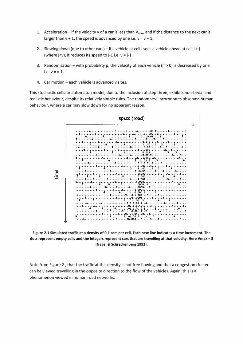
This stochastic cellular automaton model, due to the inclusion of step three, exhibits non-trivial and

realistic behaviour, despite its relatively simple rules. The randomness incorporates observed human

behaviour, where a car may slow down for no apparent reason.

Figure 2.1 Simulated traffic at a density of 0.1 cars per cell. Each new line indicates a time increment. The

dots represent empty cells and the integers represent cars that are travelling at that velocity. Here Vmax = 5

[Nagel & Schreckenberg 1992].

Note from Figure 2., that the traffic at this density is not free flowing and that a congestion cluster

can be viewed travelling in the opposite direction to the flow of the vehicles. Again, this is a

phenomenon viewed in human road networks.

There is a clear similarity between Figure 2.2 (a) and (b) in the arrowhead shape of the two curves.

Both also peak in between 0.1 and 0.2 cars per cell, which represents the highest flow or throughput

of cars on this single road of traffic. This model has been extended with success to include two lanes

and lane changing behaviour [Nagel et al, 1998].

2.3 Traffic control using cellular automata

Currently traffic is largely controlled by pre-defined traffic light sequences that in built up areas aim

to push traffic along the main “arterial” routes of the road network. Adding time conditions for the

traffic patterns at particular times in the day and for certain days in the week can help to ease the

flow of traffic, but cannot respond to the traffic and are prescribed solutions. More intelligent traffic

control systems can be implemented via a centralised system that can input multiple information

streams and calculate an optimum response, but this relies on each information node, i.e. traffic

light, being connected to the system and for the solution to be arrived at quickly (not always

practical as the problem can become complex).

Cellular automata offer an alternative traffic control system that is, due to the very nature of cellular

automata, decentralised. This allows each traffic light set to work independently and respond in real

time to traffic fluctuations. The traffic problem therefore has moved away from a complex,

centralised optimisation approach and has become focused on adaptation [Szklarski, 2010], which

will be shown throughout this section.

2.3.1 Current traffic control methods

Traffic lights currently are usually set up to run in a cyclic or “marching” system, where in its simplest

form will have a constant cycle period, independent of time or traffic flow. Another approach is to

implement the so called “green wave” or “optim” control, where a car or set of cars stopped by a

given red traffic light, will find the subsequent lights to be green once they are given the green light

to move. This is achieved by setting the traffic lights in the direction of the stopped car to the same

cycling period plus a lag due to distance between lights. The green wave approach is very popular

with avenues that have priority over crossing streets [Brockfeld et al, 2001] and is also advantageous

Figure 2.2(a) and (b) – Both show the flow of cars per time step compared to the density of vehicles on

the road. (a) is based on a simulation using the traffic model described above and (b) is based on real

traffic information [Nagel & Schreckenberg 1992].

during rush hour, when large numbers of cars tend to travel in a single direction. However it still

relies on communication between lights and a centralised system to tell the lights at what times to

exhibit this behaviour, which is based on previous experience or a preconception of traffic flow at

that instance and does not take into account the current conditions.

2.3.2 Self organising traffic lights (SOTL)

Three alternative traffic light control systems are proposed by [Gershenson et al, 2005], the SOTL –

request, SOTL – phase and the SOTL – platoon control systems, which will be referred to without

their prefixes from now on. All three use a similar principle; that all lights keep a counter that is set

to zero when the light turns red. This counter is incremented when an approaching car is stopped, or

is going to be stopped by the given traffic light during its red phase. When the counter reaches a

specified threshold, the traffic lights change colour and cars that have been or were going to be

stopped are allowed to pass through the intersection. This underlying system exhibits self

organisation as, if one or only a few cars are waiting at an intersection, they are likely to be joined by

more cars and as each group grows the less time that they will have to spend at red lights as a large

group is likely to be given precedence at an approaching intersection. This phenomenon is called

creating “green corridors” or “platoons” and is more efficient at improving traffic flow over

homogeneously distributed cars. Platoons simplify the traffic problem and reduce oscillations in the

system by reducing the interactions between groups, as there are less groups to interact

[Gershenson, 2005].

1. Request control – The system is based upon the conditions given above. Traffic lights change

only when necessary i.e. if there are no cars approaching a given light, the partner light may

stay green.

2. Phase control – This system is the same as request control apart from the additional

constraint that the traffic lights will not be induced to change by oncoming traffic until a

minimum phase time has passed. This prevents the lights switching too frequently and

hampering the overall flow of traffic.

3. Platoon control – This system is pro-platoons and incorporates two rules for this. The first

stops a red light from turning green upon approach of car if on the crossing road there is at

least one car coming along the intersecting avenue. This is done so that a platoon is more

likely to stay together. However for a high density of vehicles this would cause jams to build

up along the intersections of passing platoons so to prevent this the first additional rule is

overlooked if there are a certain number of cars approaching an intersection.

Figure 2.3 (i) Average speed, (ii) Percentage of cars stopped & (iii) Average waiting times of various different

methods of traffic control. NB, in graph (iii) waiting times that exceed the limit of the y-axis indicate that the

traffic network has become gridlocked [Gershenson 2005].

Figure 2. clearly shows that at lower densities, the SOTL methods, often far outperform the

conventional marching and optim systems. However at higher densities the trend is reversed. Here

the request system performs worst due to its aforementioned tendencies to constantly change the

lights as at this density of traffic, multiple vehicles are coming from different directions and inducing

very frequent switching. This hampers the overall traffic flow as the switching takes time in the

model.

Platoon is the best performer over a wide range of low to medium density situations, reaching very

high average speeds due to the platoons. Here the cars stigmergically pass information between

traffic light sets. One set of traffic lights affects a cars speed and journey and may build up a platoon

and this platoon will then influence the behaviour of the next set of traffic lights by “demanding” a

light switch. It is important here to note that this platoon behaviour is not forced upon the cars by

the system, but induced, and the cars reciprocate by simulating a synchronisation between traffic

lights that produces very efficient traffic flow. However at higher densities the platoon system fails

because platoons combine too much and cause multiple jams along their length. Future work could

be done here to develop this method so that it could deal with situations that involve high density

traffic, as the Gershenson was reluctant to expand the model, preferring simple rules.

The model was expanded however to mimic further real traffic characteristics. A directional

preference was introduced to simulate rush hour traffic, traffic flow in all four directions was

considered and cars given a probability of turning at intersections. Overall however none of these

characteristic significantly changed the overall behaviour of the different traffic systems. Further

work can still be done to better our understanding of these traffic systems. The work could be

improved to include multiple lanes, different driving behaviours, lane changing behaviour, multiple

street intersections and non-homogenous streets. Another interesting condition to consider would

be how the systems cope with random delays, incorporated to simulate traffic accidents. Which

system will gridlock first on average?

The reader can get a better appreciation of how the different methods compare using an online java

application [NetLogo, 2009].

2.4 Cellular Automata in traffic summary

Cellular automata have provided efficient and realistic ways of simulating traffic flow that is

exhibited in current road networks. Nagel and Schrenkenberg’s [1992] original work has been

extended to incorporate lane changing behaviour to good success [Nagel et al 1998] but further

work could be done to characterise better different driving patterns, and different vehicles e.g.

cyclists and lorry drivers. The SOTL systems provide much better traffic throughput at low to

medium traffic densities than conventional rigid traffic control, and have the huge advantage of

being easy to implement and cheaper as there is no need for central control and traffic controllers to

modulate the frequency of traffic phases, and they adapt to the current traffic situation. However

further work needs to be done to increase their performance at high density traffic, even if this

means simply switching back to a marching phase system once a critical density is reached (this

would however have to be implemented centrally). A higher density situation is less likely to exist in

the first place as traffic is more efficiently processed in the first place so perhaps this is more of a

tweak than a major hurdle. Overall traffic flows could be increased by 10 – 30% via self-organising

traffic light systems [ScienceDaily, 2010] and if traffic lights could determine between types of

vehicles, then precedence could be given to public transport and cycling, which in turn would reduce

traffic.

3 Introduction to Evolutionary Algorithms

Evolutionary Algorithms, like all of natural computation draw on inspiration from nature to help

solve problems that traditional methods of computer science cannot solve, or solve inefficiently. All

evolutionary algorithms use the same common ideas; some form of genetic structure, a system for

determining success for each generation and mutation on the genetic structures. The genetic

structure somehow maps to what the data that needs to be “evolved”, this is mixed with other areas

of evolutionary theory such as natural selection (in the form of fitness functions) and genetic cross

over. Evolutionary Algorithms are good for problems where there is a base to build up on, as the

base can be used as the first generation and anything evolved after that will be an improvement on

that base.

3.1 Salt Routing Optimisation

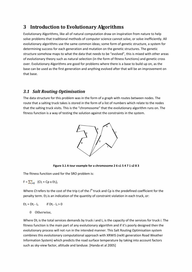
The data structure for this problem was in the form of a graph with routes between nodes. The

route that a salting truck takes is stored in the form of a list of numbers which relate to the nodes

that the salting truck visits. This is the “chromosome” that the evolutionary algorithm runs on. The

fitness function is a way of testing the solution against the constraints in the system.

Figure 3.1 A tour example for a chromosome 2 6 s1 5 4 7 1 s2 8 3

The fitness function used for the SRO problem is:

F = (Cti + Cp x Eti),

Where Ct refers to the cost of the trip ti of the ith

truck and Cp is the predefined coefficient for the

penalty term. Eti is an indication of the quantity of constraint violation in each truck, or:

Eti = Dti - Li if Dti - Li > 0

0 Otherwise,

Where Dti is the total services demands by truck i and Li is the capacity of the services for truck i. The

fitness function is the main part of any evolutionary algorithm and if it’s poorly designed then the

evolutionary process will not run in the intended manner. This Salt Routing Optimisation system

combines this evolutionary computational approach with XRWIS (neXt generation Road Weather

Information System) which predicts the road surface temperature by taking into account factors

such as sky-view factor, altitude and landuse. [Handa et al 2005]

The only possible problem with this system is that the routes will be completely different for each

time the trucks need to salt the road network, so once an optimised solution is found; it is

improbable that that solution will be suitable for later use. This means whenever the need for an

optimised route arises, the algorithm will have to run which could take a significant amount of time.

3.2 Adaptive Traffic Control

This is a problem involving the flow of traffic and offers a solution that uses evolutionary computing

in a multi-agent system. The project actually uses a machine learning technique based on an LCS

(Learning Classifier System), which is a type of evolutionary algorithm. Learning Classifier Systems

evolve rules that consist of conditions and actions (similar to if... then... clauses). The Learning

Classifier System is used with a microscopic simulation model SIGSIM, which is used to simulate the

movement of vehicles in a signal-controlled road network (i.e. traffic lights). The Learning Classifier

System is used to develop signal control strategies and test the efficiency of the solution by using

data and measures of performance generated by SIGSIM simulations. The fitness function for this

project takes into account parameters such as: delay to vehicles, capacity of critical streams and

junctions, queue lengths, and characteristics of the signal timings.

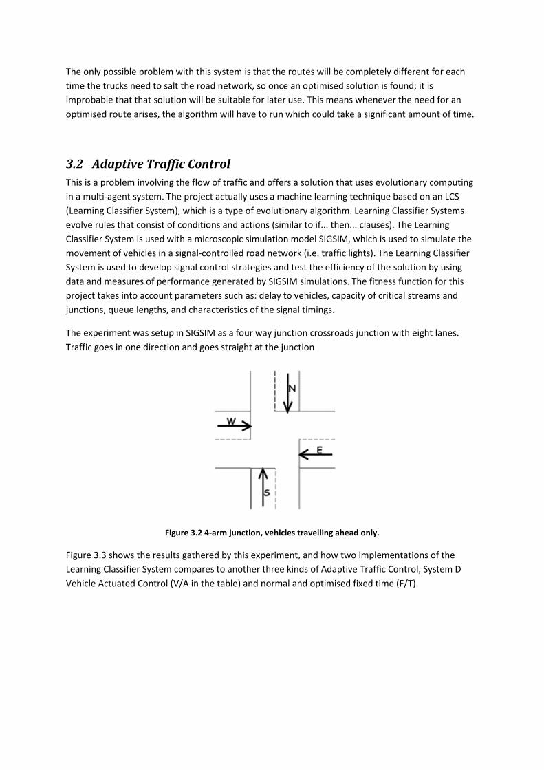
The experiment was setup in SIGSIM as a four way junction crossroads junction with eight lanes.

Traffic goes in one direction and goes straight at the junction

Figure 3.2 4-arm junction, vehicles travelling ahead only.

Figure 3.3 shows the results gathered by this experiment, and how two implementations of the

Learning Classifier System compares to another three kinds of Adaptive Traffic Control, System D

Vehicle Actuated Control (V/A in the table) and normal and optimised fixed time (F/T).

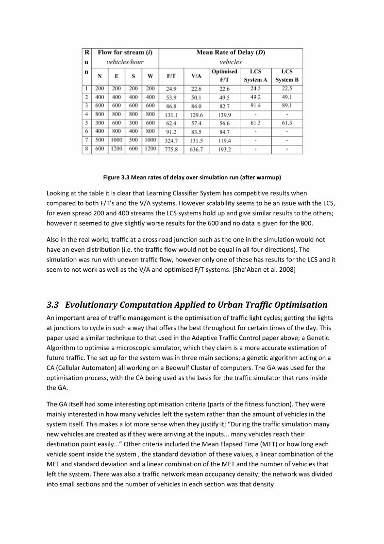
Figure 3.3 Mean rates of delay over simulation run (after warmup)

Looking at the table it is clear that Learning Classifier System has competitive results when

compared to both F/T’s and the V/A systems. However scalability seems to be an issue with the LCS,

for even spread 200 and 400 streams the LCS systems hold up and give similar results to the others;

however it seemed to give slightly worse results for the 600 and no data is given for the 800.

Also in the real world, traffic at a cross road junction such as the one in the simulation would not

have an even distribution (i.e. the traffic flow would not be equal in all four directions). The

simulation was run with uneven traffic flow, however only one of these has results for the LCS and it

seem to not work as well as the V/A and optimised F/T systems. [Sha’Aban et al. 2008]

3.3 Evolutionary Computation Applied to Urban Traffic Optimisation

An important area of traffic management is the optimisation of traffic light cycles; getting the lights

at junctions to cycle in such a way that offers the best throughput for certain times of the day. This

paper used a similar technique to that used in the Adaptive Traffic Control paper above; a Genetic

Algorithm to optimise a microscopic simulator, which they claim is a more accurate estimation of

future traffic. The set up for the system was in three main sections; a genetic algorithm acting on a

CA (Cellular Automaton) all working on a Beowulf Cluster of computers. The GA was used for the

optimisation process, with the CA being used as the basis for the traffic simulator that runs inside

the GA.

The GA itself had some interesting optimisation criteria (parts of the fitness function). They were

mainly interested in how many vehicles left the system rather than the amount of vehicles in the

system itself. This makes a lot more sense when they justify it; “During the traffic simulation many

new vehicles are created as if they were arriving at the inputs... many vehicles reach their

destination point easily...” Other criteria included the Mean Elapsed Time (MET) or how long each

vehicle spent inside the system , the standard deviation of these values, a linear combination of the

MET and standard deviation and a linear combination of the MET and the number of vehicles that

left the system. There was also a traffic network mean occupancy density; the network was divided

into small sections and the number of vehicles in each section was that density

Minimising the MET however gave undesired effects; it ended up giving good values but for the

wrong reasons. Chromosomes that blocked the network faster were favoured, resulting in “false”

optimisation cycle combinations. The chromosomes related to the combinations of the traffic lights

and the aim was to optimise the duration of a predetermined cycle of light settings. They chose to

use Gray Encoding, which is a form of bit string encoding used a lot in evolutionary computing. This

is because when mutation occurs, or when a bit changes the stage length value increases/decreases

by one unit only. (Stage length refers to the light being in a certain state for a certain amount of

time) There are many methods to choosing which individuals go through to the next generation in

evolutionary computation. This system combined Elitism and Truncation, Elitism is when the

generation is run through the fitness function and sorted in terms of fitness and only the top section

are cloned to the next generation. Truncation is where the individuals are again ranked by fitness

but then split into two section, one survives and the other is discarded. [Sanchez et al. 2008]

3.4 Decentralised Car Traffic Control Using Message Propagation

This paper had a very interesting approach to solving the traffic problem in society today, optimising

throughput at junctions and reducing the overall travel time of vehicles on the road. The system

works on the idea of message propagation between different road elements; such as road junctions,

traffic lights and even the vehicles themselves. The system used a genetic algorithm to help optimise

itself using a fitness function. The GA actually generates the parameters for the simulation rather

than optimising the running of the simulation. The prototype system consisted of 2 types of vehicles,

normal and emergency (such as fire engines, ambulances and police cars) and 2 types of message

speed-up and slow-down. The main system that the paper focuses on has much more functionality

for example re-routing traffic in times of congestion. Also the messages were changed from speed-

up/slow-down to go/stop in the terms of traffic lights rather than vehicle speed. This helped

optimise traffic in congested conditions.

The size of the simulation was very large compared to others; the system’s area was modelled as a

20 x 20 node system which represented a 2km x 2km city. Each node was an intersection with a set

of traffic light attached to it, and lines connected them were lanes with a direction, with 8 lanes

connected to each node (i.e. a crossroad junction). The simulation consisted of ~15,000 vehicles

travelling along ~1,500 interconnected lanes. The simulation started with a small number of vehicles

in random places in the system, which then targeted a location on the opposite side and deduced an

optimal route. This provides congestion to some routes from the start, the vehicles loop through

completing routes and starting new ones until the simulation is over. The fitness of a solution is

determined by the throughput of the system, or the most number of completed journeys in a fixed

amount of time (half an hour of virtual activity). The vehicles re-evaluate their route whenever they

wish and use a path finding algorithm that has parameters from the GA.

The message propagation was between the traffic junctions to request signal changes depending on

the current traffic situation, this happened in both directions. Lanes can send messages forward to

request signal changes, for example if there is a lot of stationary traffic in that lane. Backwards

message propagation is also used by lanes in cases where the lane is congested, effectively closing

the lane. Nodes cycle a token between inbound lanes to grant access to outbound lanes.

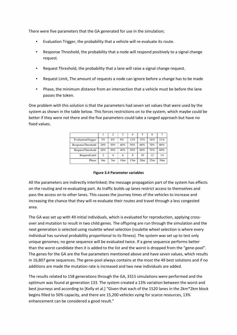
There were five parameters that the GA generated for use in the simulation;

• Evaluation Trigger, the probability that a vehicle will re-evaluate its route.

• Response Threshold, the probability that a node will respond positively to a signal change

request.

• Request Threshold, the probability that a lane will raise a signal change request.

• Request Limit, The amount of requests a node can ignore before a change has to be made

• Phase, the minimum distance from an intersection that a vehicle must be before the lane

passes the token.

One problem with this solution is that the parameters had seven set values that were used by the

system as shown in the table below. This forces restrictions on to the system, which maybe could be

better if they were not there and the five parameters could take a ranged approach but have no

fixed values.

Figure 3.4 Parameter variables

All the parameters are indirectly interlinked; the message propagation part of the system has effects

on the routing and re-evaluating part. As traffic builds up lanes restrict access to themselves and

pass the access on to other lanes. This causes the journey times of the vehicles to increase and

increasing the chance that they will re-evaluate their routes and travel through a less congested

area.

The GA was set up with 49 initial individuals, which is evaluated for reproduction, applying cross-

over and mutation to result in two child genes. The offspring are run through the simulation and the

next generation is selected using roulette wheel selection (roulette wheel selection is where every

individual has survival probability proportional to its fitness). The system was set up to test only

unique genomes; no gene sequence will be evaluated twice. If a gene sequence performs better

than the worst candidate then it is added to the list and the worst is dropped from the “gene-pool”.

The genes for the GA are the five parameters mentioned above and have seven values, which results

in 16,807 gene sequences. The gene-pool always contains at the most the 49 best solutions and if no

additions are made the mutation rate is increased and two new individuals are added.

The results related to 158 generations through the GA, 3315 simulations were performed and the

optimum was found at generation 133. The system created a 13% variation between the worst and

best journeys and according to [Kelly et al.] “Given that each of the 1520 lanes in the 2km*2km block

begins filled to 50% capacity, and there are 15,200 vehicles vying for scarce resources, 13%

enhancement can be considered a good result.”

Figure 3.5 Global results

The choice of starting off with such a congested system makes sense, as [Kelly et al.] wished to show

that message propagation and re-routing could help ease congestion in an urban environment.

Out of the four papers this one seems the most promising and realistic. The parts of the system all

work together and there seems to be a lot of potential for future work. Cars that speak wirelessly to

traffic lights and self control the traffic between them seems like an idea that could be a reality in

the not so distant future [Kelly et al. 2007].

4 Ant Colony Optimisation

Throughout the world, optimal traffic routing is becoming more and more important as the number

of cars on the roads increases. As a result, road systems which were designed for capacities much

smaller than those observed today are unable to cope. In 2008 Rod Eddington estimated that for the

UK, “unless we take action, congestion would cost us an extra £22 billion in wasted time by 2025”

[National Archives, 2008]. One approach to dealing with the increase in traffic is to develop

innovative ways to plan routes. Current research is particularly aimed at the nature inspired

technique of Ant Colony Optimisation.

Ant Colony Optimisation takes advantage of the stigmergic behaviour of ants to find approximate

solutions to difficult optimisation problems. This form of optimisation is inspired by the simple trail-

laying and -following behaviour of ants and was studied by Goss et. al. [1989]. Similarly to Cellular

Automata, Ant Colony Optimisation takes advantage of the simple behaviour of individual agents in

a large population which produces global behaviours much more complex than the rules of the

individual.

The main behaviour used to solve optimisation problems is the route finding technique that ants use

to optimise the shortest route between their nest and a food source. In nature, ants wander

randomly around and upon finding food, return to their nest while laying a down pheromone trail. If

another ant finds this trail there is a chance they will stop wandering randomly and follow the trail. If

they find food, they will return to the nest and reinforce the trail with their own pheromones.

Goss et. al. [1989] produced an experiment that demonstrated this ability in scientific setting. Their

experiment consisted of two trays: one containing a colony of ants and the second containing a food

source. The only path between the two trays was a bridge designed to provide the ants with a range

of routes, but only one shortest route and with no bias to a particular route (as shown in Figure 4.1) .

They found that the shortest route was developed using the following process:

1. The first ants arrive, choose randomly and travel along their chose branch, marking with

pheromone as they go.

2. After 20 s (the time it takes to travel the shortest path to the food), the short path will be

marked not only by ants arriving from the nest, but also by the first ants returning to the

Figure 4.1 (a) the design of the bridge between food and nest, photos taken at 4 (b) and 8 (c) minutes

after the placement of the bridge [Goss et. al. 1989].

nest that chose the short branch.

3. At this point the short branch accumulates an advantage over the long branch at both ends,

an effect which is amplified by the autocatalytic nature of the choose-and-mark process.

Thus, the short branch becomes rapidly preferred.

Whilst the ants do not communicate directly, they alter the environment to notify the rest of the

colony of the location of a food source. This behaviour is called stigmergy and it is a fundamental

part of the problem solving technique.

In computer science this method provides an excellent basis for an optimisation algorithm. The use

of multiple agents with simple rules makes modelling complex behaviour much simpler, and the

stigmergic behaviour of the optimisation technique allows the current status of the model to be

stored at each time step. For these reasons and due to the simplicity of the optimisation technique it

is often used to solve a range of Vehicle Routing Problems.

4.1 Vehicle Routing Problems Vehicle Routing Problems requires the determination of an optimal set of routes for a fleet of

vehicles that needs to serve a set of customers [Balserio, Loiseau and Ramonet, 2011]. In addition to

find the optimal route, these problems can have a range of constraints including limits on the

capacity of the vehicles, time windows for the customers to be served, and limits on the time a

driver can work or on the lengths of the routes.

A study by Balserio, Loiseau and Ramonet [2011] dealt with a vehicle routing problem where a set of

customers must be served by a fleet of vehicles located in a single depot. The problem was modelled

on a large metropolitan where travel times vary. That is, the time taken to travel between two

points does not depend solely on the distance: traffic fluctuations seriously affect travel speeds,

resulting in great variations in travel times. Other constraints included allowing the clients to impose

time windows during which they can be served. A vehicle can arrive before the beginning of the

window but is not permitted to begin serving them until the start of the window or after the end.

The capacity of the vehicles was also limited in this study.

In order to solve the vehicle routing problem with this range of constraints, Balserio, Loiseau and

Ramonet [2011] use a Multiple Ant Colony System. This uses a pair of ant colonies to optimise the

two main solutions. The first colony (ACS-TIME) optimises the best total time solution with the given

number of vehicles v, whilst the colony ACS-VEI tries to minimise the number of vehicles by

minimizing the number of unrouted clients in solutions with v-1 vehicles. These are optimised in

order of priority: (1) ACS-VEI and (2) ACS-TIME. A solution that employs fewer vehicles is better than

another that uses more in spite of total time. Only when two solutions have an equal number of

routes are their times compared. This objective is typical of Vehicle Routing Problems because the

fixed cost of drivers and vehicles usually has a “greater impact than per-mile transportation costs”

[Balserio, Loiseau and Ramonet, 2011].

4.1.1 Representation and Evaluation

Ant Colony optimisation is typically represented by a graph in which nodes are connected by edges.

Each edge has a probability that it will be travelled by an ant and this probability represents the

pheromone trail lain down by the ants. In this study, the probability pij that an ant will move to client

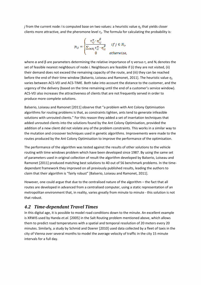
j from the current node i is computed base on two values: a heuristic value ηij that yields closer

clients more attractive, and the pheromone level τij. The formula for calculating the probability is:

where α and β are parameters determining the relative importance of η versus τ, and Ni denotes the

set of feasible nearest neighbours of node i. Neighbours are feasible if (i) they are not visited, (ii)

their demand does not exceed the remaining capacity of the route, and (iii) they can be reached

before the end of their time window [Balserio, Loiseau and Ramonet, 2011]. The heuristic value ηij

varies between ACS-VEI and ACS-TIME. Both take into account the distance to the customer, and the

urgency of the delivery (based on the time remaining until the end of a customer’s service window).

ACS-VEI also increases the attractiveness of clients that are not frequently served in order to

produce more complete solutions.

Balserio, Loiseau and Ramonet [2011] observe that “a problem with Ant Colony Optimisation

algorithms for routing problems is that, as constraints tighten, ants tend to generate infeasible

solutions with unrouted clients.” For this reason they added a set of insertation techniques that

added unrouted clients into the solutions found by the Ant Colony Optimisation, provided the

addition of a new client did not violate any of the problem constraints. This works in a similar way to

the mutation and crossover techniques used in genetic algorithms. Improvements were made to the

routes produced by the Ant Colony Optimisation to improve the performance of the optimisation.

The performance of the algorithm was tested against the results of other solutions to the vehicle

routing with time windows problem which have been developed since 1987. By using the same set

of parameters used in original collection of result the algorithm developed by Balserio, Loiseau and

Ramonet [2011] produced matching best solutions to 40 out of 56 benchmark problems. In the time-

dependant framework they improved on all previously published results, leading the authors to

claim that their algorithm is “fairly robust” [Balserio, Loiseau and Ramonet, 2011].

However, one could argue that due to the centralised nature of the algorithm – the fact that all

routes are developed in advanced from a centralised computer, using a static representation of an

metropolitan environment that, in reality, varies greatly from minute to minute - this solution is not

that robust.

4.2 Time-dependant Travel Times In this digital age, it is possible to model road conditions down to the minute. An excellent example

is XRWIS used by Handa et.al. [2005] in the Salt Routing problem mentioned above, which allows

them to predict road temperatures with a spatial and temporal resolution of 20 meters every 20

minutes. Similarly, a study by Schmid and Doerer [2010] used data collected by a fleet of taxis in the

city of Vienna over several months to model the average velocity of traffic in the city 15 minute

intervals for a full day.

Although these studies do not deal specifically with Ant Colony Optimisation, they do lead the way in

using dynamic and up-to-date data to produce optimal solutions to routing problems. The study by

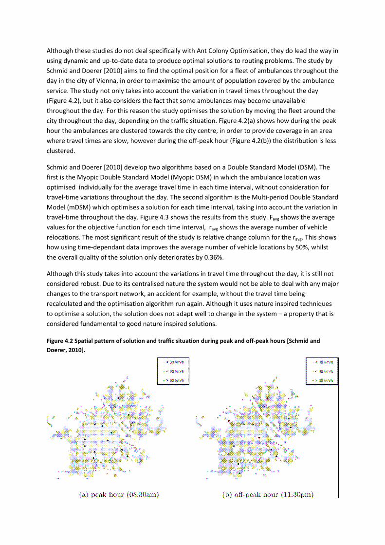
Schmid and Doerer [2010] aims to find the optimal position for a fleet of ambulances throughout the

day in the city of Vienna, in order to maximise the amount of population covered by the ambulance

service. The study not only takes into account the variation in travel times throughout the day

(Figure 4.2), but it also considers the fact that some ambulances may become unavailable

throughout the day. For this reason the study optimises the solution by moving the fleet around the

city throughout the day, depending on the traffic situation. Figure 4.2(a) shows how during the peak

hour the ambulances are clustered towards the city centre, in order to provide coverage in an area

where travel times are slow, however during the off-peak hour (Figure 4.2(b)) the distribution is less

clustered.

Schmid and Doerer [2010] develop two algorithms based on a Double Standard Model (DSM). The

first is the Myopic Double Standard Model (Myopic DSM) in which the ambulance location was

optimised individually for the average travel time in each time interval, without consideration for

travel-time variations throughout the day. The second algorithm is the Multi-period Double Standard

Model (mDSM) which optimises a solution for each time interval, taking into account the variation in

travel-time throughout the day. Figure 4.3 shows the results from this study. Favg shows the average

values for the objective function for each time interval, ravg shows the average number of vehicle

relocations. The most significant result of the study is relative change column for the ravg. This shows

how using time-dependant data improves the average number of vehicle locations by 50%, whilst

the overall quality of the solution only deteriorates by 0.36%.

Although this study takes into account the variations in travel time throughout the day, it is still not

considered robust. Due to its centralised nature the system would not be able to deal with any major

changes to the transport network, an accident for example, without the travel time being

recalculated and the optimisation algorithm run again. Although it uses nature inspired techniques

to optimise a solution, the solution does not adapt well to change in the system – a property that is

considered fundamental to good nature inspired solutions.

Figure 4.2 Spatial pattern of solution and traffic situation during peak and off-peak hours [Schmid and

Doerer, 2010].

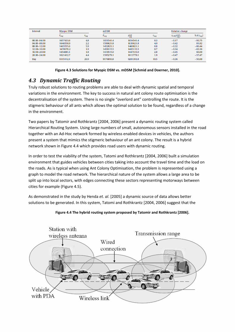
Figure 4.3 Solutions for Myopic DSM vs. mDSM [Schmid and Doerner, 2010].

4.3 Dynamic Traffic Routing Truly robust solutions to routing problems are able to deal with dynamic spatial and temporal

variations in the environment. The key to success in natural ant colony route optimisation is the

decentralisation of the system. There is no single “overlord ant” controlling the route. It is the

stigmeric behaviour of all ants which allows the optimal solution to be found, regardless of a change

in the environment.

Two papers by Tatomir and Rothkrantz [2004, 2006] present a dynamic routing system called

Hierarchical Routing System. Using large numbers of small, autonomous sensors installed in the road

together with an Ad-Hoc network formed by wireless enabled devices in vehicles, the authors

present a system that mimics the stigmeric behaviour of an ant colony. The result is a hybrid

network shown in Figure 4.4 which provides road users with dynamic routing.

In order to test the viability of the system, Tatomi and Rothkrantz [2004, 2006] built a simulation

environment that guides vehicles between cities taking into account the travel time and the load on

the roads. As is typical when using Ant Colony Optimisation, the problem is represented using a

graph to model the road network. The hierarchical nature of the system allows a large area to be

split up into local sectors, with edges connecting these sectors representing motorways between

cities for example (Figure 4.5).

As demonstrated in the study by Henda et. al. [2005] a dynamic source of data allows better

solutions to be generated. In this system, Tatomi and Rothkrantz [2004, 2006] suggest that the

Figure 4.4 The hybrid routing system proposed by Tatomir and Rothkrantz [2006].

vehicles themselves provide data for the routing system by communicating their route and the time

it took to travel each section to the Hierarchical Routing System. This allows the travel time for each

edge to be stored in probability tables which a “smart vehicle,” as described in this study, will have

access to when planning a route.

A simulation environment was built to allow Tatomi and Rothkrantz [2006] to test the

responsiveness of the system to changes in travel time. The simulation used a skeleton road network

with four cities connected by motorways, and 4 vehicle categories:

1. Vehicles that have no communication with the routing system and are guided by a regular

route finding algorithm;

2. Vehicles that give information about the state of the traffic system but do not use it (e.g.

public transport);

3. Vehicles that give no information, but do use it for routing;

4. Vehicles that use the routing system and also provide it with information.

Categories one and two are called ‘standard vehicles’ and categories three and four are called ‘smart

vehicles.’ The simulation is run for a period of time to allow the system to “warm up” and collect

data about road use. After 2500 time steps an accident is generated between two cities by artificially

reducing the speed down to 20km/h on that edge. The results can be seen in Figure 4.6.

Figure 4.5 A network model used by Tatomir and Rothkrantz [2006].

Figure 4.6 The results of the Heirarchical Routing System for standard vehicles (left) and smart vehicles

(right) [Tatomir and Rothkrantz, 2006].

Although the trip time of the smart vehicles increases rapidly, it only increases the trip time by about

300 time steps, whilst the standard vehicle trip time increases by at least 1000 time steps. At 10000

time steps an additional delay is added to the road network. This only costs the smart vehicles an

additional ~150 units of time, whilst the standard vehicle trip time increases by a further 500 units.

At time 15000 the original block is released. It is clear that the standard vehicles respond most

rapidly to this change in the system, but once the smart vehicles notice the change in the system

they also begin to reuse this route.

5 Conclusion

Throughout the research in this area, it has become clear that current traffic systems are inefficient,

often over complicated and too centralised. A decentralised system that can respond dynamically to

the current traffic state is preferred, over one that has been carefully prepared, based on average

data observations, but is more rigid. This is due to the inherent random or naturally fluctuating

behaviour of traffic that is exhibited because of our human nature.

It is clear from these studies that the most robust solutions are those that take into account the

dynamic changes in the environment and are able to adapt to them on the fly. Implementing the

solution proposed by Tatomi and Rothkrantz [2006]would be expensive, but not difficult. Road side

sensors could be added with ease and the wireless units in the cars could be developed alongside

existing GPS solutions such as the TomTom or NavMan which are commonly used today. It is also

important to consider the economic impact of implementing this solution. The smart vehicles travel

times were seven times shorter than the standard vehicles and although this would not correlate to

similar reduction in the cost of congestion, the savings would still be considerable.

The dynamic traffic routing method described in the ant algorithm section, the SOTL method in the

cellular automata section and the message propagation method in the evolutionary algorithm

section are all decentralised and show the most promise. Future work should focus on developing

these ideas, that the cars and traffic lights should interact independently of a central control unit,

and more complex models be tested. It would also be interesting to develop all three good solutions

into a single solution and evaluate the effectiveness of multiple systems working together. The fact

that all these solutions use simple rules should not make it difficult to integrate them into a single

solution, however the cost of evaluation may be considerable.

Finally, although projects have been implemented on real road networks in some cases [Gershenson,

2005], these have largely been carried out on isolated or small areas. Implementation in a city or

over a large area, would advance this field significantly.

6 References

Balserio, S. R., Loiseau, I. and Ramonet, J., 2011. An Ant Colony algorithm hybridized with insertation

heuristics for the Time Dependen Vehicle Routing Problem with Time Windows. Computers

& Operation Research, 38, 954 – 966.

Biham, O, Middleton, A.A and Levine D, 1992. Self-organization and a dynamical transition in traffic-

flow models.

Boccara, N & Fuks, H, 1998. Cellular automaton rules conserving the number of active sites.

Adaptation and Self-Organizing Systems. Journal of Physics A: Mathematical and Theoretical.

Brockfeld, E et al 2001. Optimizing traffic lights in a cellular automaton model for city traffic. Physical

review E, Vol 64.

Gershenson, C., 2005. Self-organizing Traffic Lights. Complex Systems, 16, 29-53.

Goss, S., Aron, S., Deneubourg, J. L. and Pasteels, J. M., 1989. Self-organised Shortcuts in the

Argentine Ant. Naturewissenschaften, 76, 579 – 581.

Handa, H et al. Dynamic Salting Route Optimisation using Evolutionary Computation.

Kelly, M et al, 2007. Decentralised Car Traffic using Message Propagation Optimised with a Genetic

Algorithm.

Medina, J et al, 2008. Evolutionary Computation Applied to Urban Traffic Optimisation. Advances in

Evolutionary Algorithms.

Nagel, K and Schreckenberg, M., 1992. A cellular automaton model for freeway traffic. Journal de

physique I, page 2221-2229.

Nagel, K et al., 1998. Two-lane traffic rules for cellular automata: A systematic approach. Physical

Review E, Vol. 58 No. 2

National Archives, 2008. Delivering choice and reliability [Online]. Available at

<http://webarchive.nationalarchives.gov.uk/+/http://www.dft.gov.uk/press/speechesstate

ments/speeches/congestion> [Accessed 6 March 2011].

NetLogo, 2009. A model of city traffic based on elementary cellular automata [Online]. Available at

<http://turing.iimas.unam.mx/~cgg/NetLogo/trafficCA.html> [Accessed 5 March 2011].

Quartieri, J et al, 2010. Cellular Automata Application to Traffic Noise Control. Automatic Control,

Modelling & Simulation. 12th

WSEAS International Conference.

Schmid, V. and Doerner, K. F., 2010. Ambulence location and relocation problems with time-

dependent travel times. European Journal of Operational Research, 207, 1293 – 1301.

ScienceDaily, 2010. Self-Organizing Traffic Lights. ScienceDaily [Online]. Available at:

<http://www.sciencedaily.com/releases/2010/09/100915094416.htm> [Accessed 4 March

2011].

Sha’Aban, J et al, 2008. Adaptive Traffic Control using Evolutionary Algorithms.

Szklarski, J., 2010. Cellular automata model of self-organizing traffic control in urban networks.

Bulletin of the polish academy of sciences, Technical sciences, Vol 58, No. 3.

Tatomir, B. and Rothkrantz, L., 2004. Dynamic traffic routing using Ant Based Control. IEEE

International Conference on Systems, Man and Cybernetics.

Tatomir, B. and Rothkrantz, L., 2006. Hierarchical routing in traffic using swarm-intelligence. IEEE

Intelligent Transport Systems Conference, Toronto, Canada, September 17 – 20, 2006.

Wolfram, S, 1986. Theory and Applications of Cellular Automata. World Scientific, Singapore.