transportation energy –what is best?
TRANSCRIPT

Transportation Energy – What is Best?
Mark DelucchiResearch Scientist
Transportation Sustainability Research CenterInstitute of Transportation StudiesUniversity of California, Berkeley
IEE SeminarUC Santa Barbara
April 27, 2017

Outline
• What I mean by “best?”• What do we care about – what are we trying to fix?
– Some external costs in the US– Global trends in air pollution, water use, nutrient discharge, biodiversity
• Qualitative evaluation of solutions to transport problems• Quantitative comparison of some alternatives for LDVs
– Water consumption of alternative-fuel LDVs– Land use of alternative-fuel vehicles– CO2-equivalent lifecycle GHGs from biofuel LDVs– Social lifetime cost of alternative-fuel LDVs
• Comments on other modes• The context for considering solutions
– The changing energy context– The radically changing social context
• What are the important research questions?• Summary and conclusions

What do we – I – mean by “best?”
• Qualitatively: maximize the potential for long-term human welfare, with an emphasis on the well-being of the least well-off and on the sustainability of all earth’s ecosystems – at least (or acceptable) cost
• Consider a wide range of evaluation criteria
• This is not necessarily the same as maximizing net benefits in a traditional social-cost benefit analysis:
– Takes a longer term view, with low (near-zero) “discount rate”– Does not trade-off rich-person “amenity” values with impacts on human health,
education, and basic opportunity

Measuring the problems: external costs of motor-vehicle use, U.S., 1990 (109 1991 $)
Cost item Low High Q
Accidental pain, suffering, and death 30 120 A3, D
Travel delay, imposed by other drivers that displaces unpaid activities 35 140 A2
Air pollution: human health impacts from motor-vehicle emissions 19.3 283 A1
Air pollution: human health impacts from upstream emissions, road dust 5.3 167 A1
Air pollution: damages to visibility, crops, materials, and forests 7.8 50.9 B-A1
Climate change due to fuel-cycle emissions of GHGs (U. S. /global damages) 0.0 /2.4 3.5 /25.2 A1, B
Noise from motor vehicles 0.5 15 A1
Water pollution: oils spills, fuel leaks, urban runoff, road de-icing 2.8 7.3 C,D
Expected loss of GNP due to sudden changes in the price of oil 1.6 25 C [A1]
Pecuniary cost increased payments to foreign countries for non-transport oil 4.0 8.4 A3
Strategic Petroleum Reserve, military expenditures related to oil use 0.7 8.0 A3
Source: estimates for entire in-use highway fleet in 1990 from Delucchi (2008). SCC is $1-$10 metric-tonne-CO2e for global damages, $0-1.40 US.Q = qaulity of the estimate.

MV external costs in the US: the business-as-usual future
Recent past Future
VMT Per mile Exposure, Effects Unit Value
Accidents é é? ê êê* − ê − ê é é
Congestion é é? − − − − é é
Air pollution é é? ê ê é é é é
Climate change é é? − ê é é é^ é^
Energy use é é? − ê é é é é
Noise é é? − − ? ? é é
*With widespread vehicle automation. ^Improved methods have increased SCC by an order of magnitude
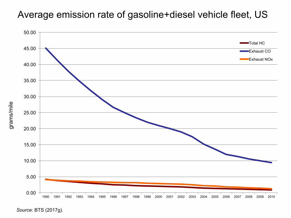
Average emission rate of gasoline+diesel vehicle fleet, US
Source: BTS (2017g).
0.00
5.00
10.00
15.00
20.00
25.00
30.00
35.00
40.00
45.00
50.00
1990 1991 1992 1993 1994 1995 1996 1997 1998 1999 2000 2001 2002 2003 2004 2005 2006 2007 2008 2009 2010
gram
s/m
ile
Total HC
Exhaust CO
Exhaust NOx

PM2.5, NOx, highway vehicles and total, w.r.t 1990, US
Source: USEPA (2017b)
0.00
0.20
0.40
0.60
0.80
1.00
1.20Highway vehicles PM2.5All sources PM2.5Highway vehicles NOxAll sources NOx
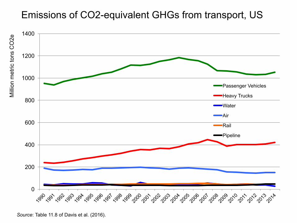
Emissions of CO2-equivalent GHGs from transport, US
Source: Table 11.8 of Davis et al. (2016).
0
200
400
600
800
1000
1200
1400
Milli
on m
etric
tons
CO
2e
Passenger Vehicles
Heavy Trucks
Water
Air
Rail
Pipeline
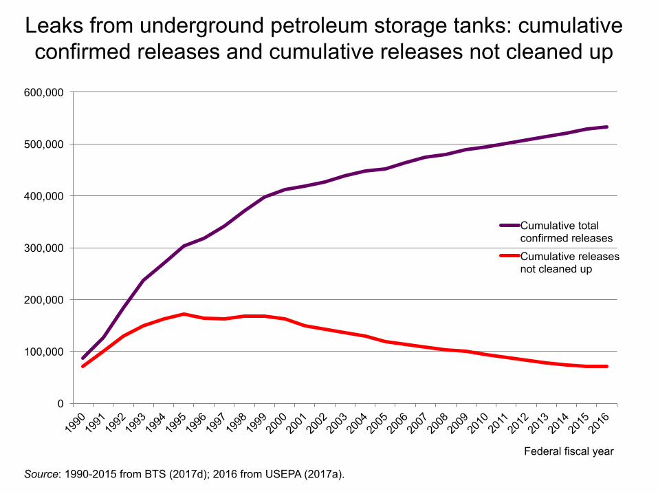
Leaks from underground petroleum storage tanks: cumulative confirmed releases and cumulative releases not cleaned up
Source: 1990-2015 from BTS (2017d); 2016 from USEPA (2017a).
0
100,000
200,000
300,000
400,000
500,000
600,000
Federal fiscal year
Cumulative total confirmed releasesCumulative releases not cleaned up

Petroleum spills impacting navigable US waterways
Source: BTS (2017e). Note: 2010 is 207-million-gallon Deepwater Horizon blowout.
0
1,000,000
2,000,000
3,000,000
4,000,000
5,000,000
6,000,000
7,000,000
8,000,000
9,000,000
10,000,000
1995 1996 1997 1998 1999 2000 2001 2002 2003 2004 2005 2006 2007 2008 2009 2010 2011 2012 2013 2014 2015
gallo
ns Total, all spills
Vessel sources, total

Highway noise barrier construction in the US
Source: BTS (2017f).
0
50
100
150
200
250
300
350
400
1990 1991 1992 1993 1994 1995 1996 1997 1998 1999 2000 2001 2002 2003 2004 2005 2006 2007 2008 2009 2010 2011 2012 2013
mile
s or
milli
on $
Total length of barriers (miles)
Cost (million 2013 $)

Global trends in important indicators of air pollution, water use, nutrient
discharge, and biodiversity

HC and NOx emission stds for gasoline cars in OECD
Source: OECD (2012h).
0
1
2
3
4
5
6
1970 1975 1980 1985 1990 1995 2000 2005 2010
gram
s pe
r km
US HC all cars
US NOx
US HC+NOx all cars
JPN HC
JPN NOx
EUR HC
EUR NOx
EUR HC+NOx

PM2.5, NOx, mobile sources, w.r.t 1990, UK and Italy
Source: OECD (2015a).
0.00#
0.20#
0.40#
0.60#
0.80#
1.00#
1.20#
1.40#
1990# 1991# 1992# 1993# 1994# 1995# 1996# 1997# 1998# 1999# 2000# 2001# 2002# 2003# 2004# 2005# 2006# 2007# 2008# 2009# 2010# 2011# 2012#
PM2.5#road#transport,#United#Kingdom#
PM2.5#other#mobile#sources,#United#Kingdom#
NOx#road#transport,#United#Kingdom#
NOx#other#mobile#sources,#United#Kingdom#
PM2.5#road#transport,#Italy#
PM2.5#other#mobile#sources,#Italy#
NOx#road#transport,#Italy#
NOx#other#mobile#sources,#Italy#

SOx, NOx, and BC emissions by region
Source: OECD (2012i).
0
20
40
60
80
100
120
140
160
180
SO2 NOx BC SO2 NOx BC SO2 NOx BC
OECD BRIICS RoW
Emis
sion
s (in
dex
2010
= 1
00)
2010 2030 2050
SO2 NOx SO2 NOx SO2 NOx

Global premature deaths from some environmental risks
Source: OECD (2012j).
0.0 0.5 1.0 1.5 2.0 2.5 3.0 3.5 4.0
Particulate Matter
Ground-level ozone
Unsafe Water Supply and Sanitation*
Indoor Air Pollution
Malaria
Deaths (millions of people)
2010
2030
2050

Global mortality from fossil-fuel air-pollution in 2050
Country High Middle Low
India 1,667,221 805,227 195,433
China 1,380,050 638,165 148,273
Nigeria 984,287 514,900 132,376
Pakistan 361,391 180,243 44,816
Bangladesh 280,467 130,598 30,780
Russian Federation 225,543 102,559 23,534
Ethiopia 182,850 78,819 17,493
Sudan 151,527 72,899 17,302
United States of America 103,679 45,761 11,734
Egypt 89,901 41,491 10,136
Subtotal top 10 5,426,915 2,610,662 631,878
Total for 139 countries 7,376,181 3,487,163 838,205
Source: Jacobson, Delucchi et al. (2017).

Source: Wada and Bierkens (2014)
Nonrenewable/total groundwater use, 1960, 2010, 2099
0%
10%
20%
30%
40%
50%
60%
70%
80%
90%
India USA China Pakistan Iran Mexico Saudi Arabia
1960
2010
2099

Source: World Bank (2017a).
Renewable internal freshwater resource (m3/capita)
0
2000
4000
6000
8000
10000
12000
1997 1999 2001 2003 2005 2007 2009 2011 2013 2015
YEAR
High-income countries
Middle-income countriesLow-income countries

Global water demand 2000 and 2050
0
1 000
2 000
3 000
4 000
5 000
6 000
2000 2050 2000 2050 2000 2050 2000 2050
OECD BRIICS RoW World
Km
3
electricity manufacturing livestock domestic irrigation
Source: OECD (2012a). See also Byers et al. (2016) on water use of CCS.
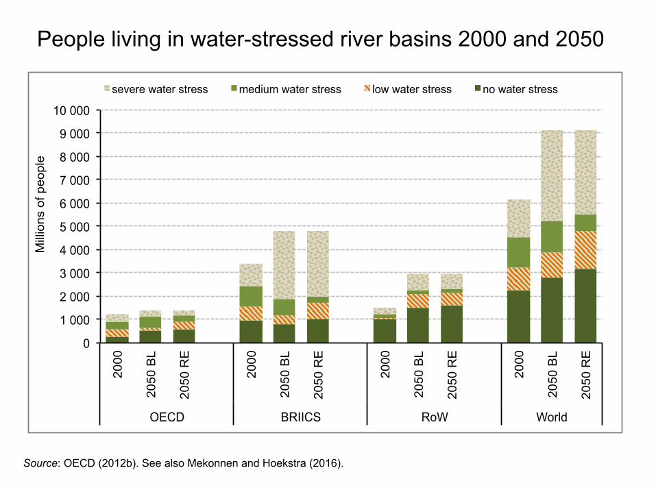
People living in water-stressed river basins 2000 and 2050
Source: OECD (2012b). See also Mekonnen and Hoekstra (2016).
0
1 000
2 000
3 000
4 000
5 000
6 000
7 000
8 000
9 000
10 000 20
00
2050
BL
2050
RE
2000
2050
BL
2050
RE
2000
2050
BL
2050
RE
2000
2050
BL
2050
RE
OECD BRIICS RoW World
Mill
ions
of p
eopl
e
severe water stress medium water stress low water stress no water stress

Global agricultural area, various estimates, to 2050
Source: OECD (2012c).
30
35
40
45
50
55
60
65
70
1980 1990 2000 2010 2020 2030 2040 2050
Agric
ultu
ral a
rea
(milli
ons
of k
m2 )
FAO/IMAGE
IAASTD
MEA scenarios
Outlook Baseline
0 -

Source: World Bank (2017b).
Fertilizer consumption (kg per ha of arable land)
0
20
40
60
80
100
120
140
160
2002 2003 2004 2005 2006 2007 2008 2009 2010 2011 2012 2013
YEAR
High-income countries
Middle-income countries
Low-income countries

River discharges of nutrients into the sea, 1950 to 2050
Source: OECD (2012d).
0
2
4
6
8
10
12
14
16
Arctic Ocean Atlantic Ocean Indian Ocean Medit + Black Sea Pacific Ocean
Mill
ion
s o
f to
nn
es
of N
pe
r ye
ar
1950 1970 2000 2030 2050

Effects of different pressures on species abundance, 2010, 2030, 2050
MSA = means species abundance as a % of species in pristine ecosystems.
Source: OECD (2012e).
50%
60%
70%
80%
90%
100%
2010 2030 2050 2010 2030 2050 2010 2030 2050 2010 2030 2050
OECD BRIICS RoW World
MS
A
Infr+Encr+Frag
Climate Change
Nitrogen
Former Land-Use
Forestry
Pasture
Bioenergy
Food Crop
Remaining MSA 0"#

Global forest area change, to 2050
Source: OECD (2012f).
75
80
85
90
95
100
105
110
115
2010 2020 2030 2040 2050
Fo
rest
co
ver
(201
0 =
100
%)
Primary Forest OECD
Primary Forest BRIICS
Primary Forest RoW
Primary Forest World
Total Forest OECD
Total Forest BRIICS
Total Forest RoW
Total Forest World

Terrestrial species abundance per biome, to 2050
MSA=means species abundance as a % of species in pristine ecosystems.
Source: OECD (2012g).
Polar/Tundra
Grassland/Steppe
Scrubland/Savanna
Boreal forests
Temperate forests
Tropical forests
Hot desert
Total MSA
0
10
20
30
40
50
60
70
80
90
100
2000 2010 2020 2030 2050
Me
an
Sp
ec
ies
Ab
un
da
nc
e (
%)

Everything is pretty bad now
Most things will get worse
It is and will be especially bad in poorer countries
SUMMING UP THE PROBLEMS

Qualitative evaluation of solutions to transport problems
Criterion Best options Comments w.r.t. to energy
AccidentsVehicle automation, mode shift, traffic
separation, travel reduction, traffic control, behavior/licensing control, vehicle safety
technology, emergency response…
Compatible with all energy systems, but some minor advantages for electric-
drive systems
CongestionMode shift, automation, travel reduction, traffic
control, pricing, expanded infrastructure, supportive land-use planning…
Compatible with all energy systems, but some (very) minor advantages for
electric-drive systems
Air pollution Zero-emission modesNeed non-combustion power source:
electrification with zero-emission primary energy
Climatechange
Zero fossil-fuel use, zero negative land-use change worldwide
Prima facie electrification with zero-emission primary energy is good, but
what about bioenergy?
Oil use Zero oil use worldwide Electrification or biofuels
Noise Low-speed vehicles; non-combustion power sources Electric-drive systems
Water use Need formal evaluation of water intensity of energy options
Biodiversity Energy and infrastructure systems with minimal land footprint in important ecosystems
Need formal evaluation, but prima facie bioenergy is worst choice
Cost Need formal evaluation. Usually it is assumed that the zero-emission options that provide the greatest social and environmental benefits are too costly, but is this correct?

Quantitative comparison: water consumption of alternative-fuel vehicles
Fuel petrol FTD H2 H2 Elec. Elec. E85 biodiesel E85
Feedstock oil NG NG WWS US grid WWS irr. CS irr. soy nirr. CS
Vehicle ICEV ICEV FCV FCV BEV BEV ICEV ICEV ICEV
gal-H2O/mi 0.10 0.27 0.065 0.035 0.25 0.005 20 10 0.26
Notes: FTD = Fischer-Tropsch Diesel, H2 = hydrogen, Elec. = electricity, E85 = 85% ethanol, NG = natural gas, WWS = wind, water, or solar power, US grid = US average electricity mix, irr. = irrigated, nirr. = not irrigated, CS = corn stover.
Source: King and Webber (2008). See also Spang et al. (2014), and Byers et al. (2016) on water use of CCS.

Area to Power 100% of U.S. Onroad Vehicles
Cellulosic E85
4.7-35.4%of US
Geoth BEV0.006-0.008%
Solar PV-BEV0.077-0.18% of US
Slide contributed by Mark Z. Jacobson, Dept. of Civil & Environmental Engineering, Stanford University
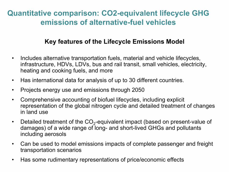
Key features of the Lifecycle Emissions Model
• Includes alternative transportation fuels, material and vehicle lifecycles, infrastructure, HDVs, LDVs, bus and rail transit, small vehicles, electricity, heating and cooking fuels, and more
• Has international data for analysis of up to 30 different countries.• Projects energy use and emissions through 2050• Comprehensive accounting of biofuel lifecycles, including explicit
representation of the global nitrogen cycle and detailed treatment of changes in land use
• Detailed treatment of the CO2-equivalent impact (based on present-value of damages) of a wide range of long- and short-lived GHGs and pollutants including aerosols
• Can be used to model emissions impacts of complete passenger and freight transportation scenarios
• Has some rudimentary representations of price/economic effects
Quantitative comparison: CO2-equivalent lifecycle GHG emissions of alternative-fuel vehicles

CO2-equivalent lifecycle GHGs from biofuel LDVs
Source: From current beta version of the Lifecycle Emissions Mode (LEM); see Delucchi et al. (2003) for documentation of a prior version.
26 mpg LDV, US year 2040, g/mi and % ∆ vs. gasoline

Quantitative comparison of some alternatives: social lifetime cost of alternative-fuel vehicles
The Advanced-Vehicle Cost and Energy-Use Model (AVCEM)
A detailed, integrated model of vehicle design, energy use, manufacturing cost, lifetime operating cost, and external costs, for H2 and methanol fuel cell vehicles, pure battery EVs, hybrid EVs, and alternative fuel ICEVs

Calculation logic of AVCEM
The Advanced-Vehicle Cost and Energy-Use Model (AVCEM):
A detailed, integrated model of vehicle design, energy use, manufacturing cost, lifetime operating cost, and external costs, for H2 and methanol fuel cell vehicles, pure battery EV, hybrid EVs, and alternative fuel ICEVs.

Studies of the social cost of carbon
IAM = Integrated Assessment Model; SCC = social cost of carbon; n.r. = not reported; part. = partially. “Extreme climate impacts?” includes extreme climate sensitivity to emissions, irreversible impacts, high-cost/low-probability impacts, and potentially large but difficult to quantify damage categories. Note that here “low” and “high refer to values of the SCC itself, and not to the LCHB and HCLB scenarios established here.

Quantitative comparison: social lifetime cost, 2020Compact car, Li-ion battery, FUDS cycle (present value of costs)
Source: Current beta version of AVCEM; see Delucchi et al. (2000) for documentation of prior version.

Comments on other modes
• Heavy trucks (inferences from results for light trucks?)
• Trains – electrify
• Ships – electrify ports; batteries and fuel cells while traveling
• Airplanes – batteries short haul? LH2? Biofuels from waste?
THE CHANGING ENERGY CONTEXT

Source: World Bank (2017d).
Access to electricity (% of population)
0
10
20
30
40
50
60
70
80
90
100
1990 1992 1994 1996 1998 2000 2002 2004 2006 2008 2010 2012 2014 2016
YEAR
High-income countries
Middle-income countries
Low-income countries

Source: World Bank (2017e).
Primary energy use per GDP (MJ/$2011 PPP GDP)
0
2
4
6
8
10
12
14
16
18
1990 1992 1994 1996 1998 2000 2002 2004 2006 2008 2010 2012 2014 2016
YEAR
High-income countries
Middle-income countries
Low-income countries
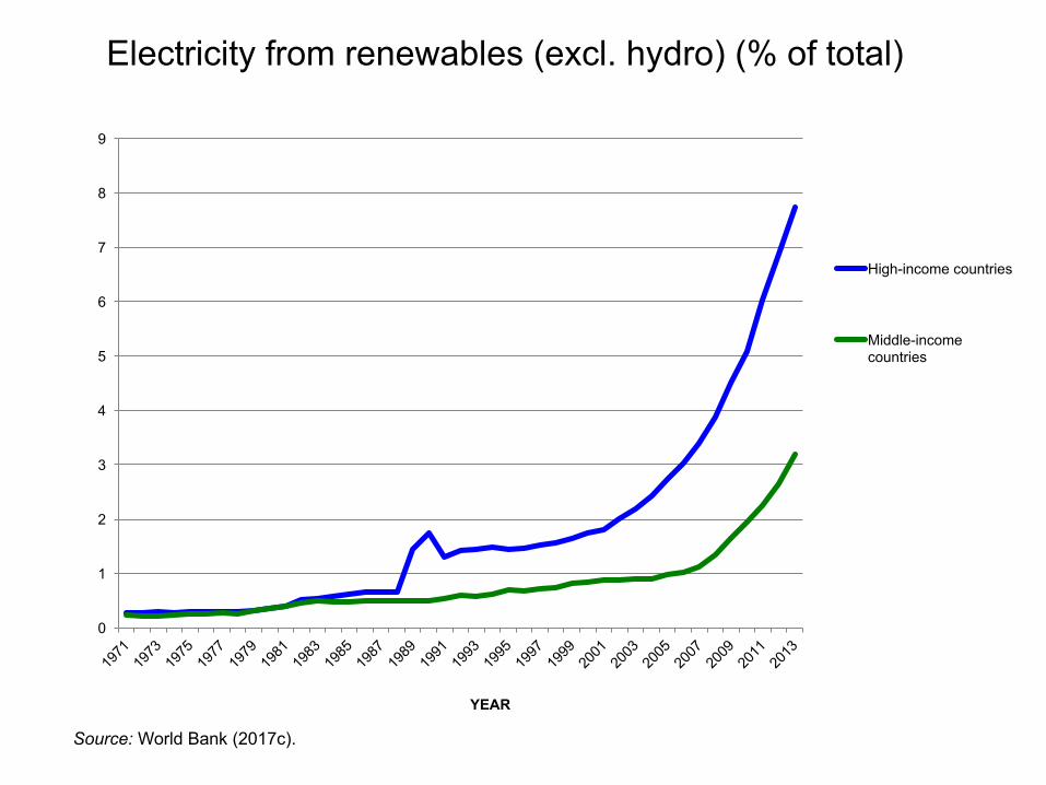
Source: World Bank (2017c).
Electricity from renewables (excl. hydro) (% of total)
0
1
2
3
4
5
6
7
8
9
YEAR
High-income countries
Middle-income countries

LCOE of WWS vs. BAU (cents/kWh in 2050)
LCOE = levelized cost of electricity; WWS = wind, water, and solar power; BAU = business as usual; LCHB = low cost, high benefits; HCLB = high cost, low benefits; T&D = transmission and distribution. Year 2013 dollars. Discount rate is 1.5% (LCHB) or 4.5% (HCLB).
Source: M. Z. Jacobson, M. A. Delucchi, et al. (2015).

THE RADICALLY CHANGING SOCIAL CONTEXT

VMT vs. GDP, Drivers, Affordability
Sources: FHWA, BEA, BTS, and others. See Appendix A for details.
0.00
0.50
1.00
1.50
2.00
2.50
60 61 62 63 64 65 66 67 68 69 70 71 72 73 74 75 76 77 78 79 80 81 82 83 84 85 86 87 88 89 90 91 92 93 94 95 96 97 98 99 0 1 2 3 4 5 6 7 8 9 10 11 12 13 14 15
w.r.t1990
YEAR
Personaldisposableincome(real)
GDP(real)
VMT-Allvehicles
VMT-LDVs
Vehiclesexcl.motorcycles
PMT-LDVs
Drivers/Pop.>16
LDVMTaffordability(milesper$fuel)

What’s going on? Younger generations like driving less and alternatives more
Source: National Association of Realtors and Portland State University (2015).

…are much less attached to having their own car…
Survey data presented by Susan Handy at the 2015 Asilomarconference indicate that:
• Millennials were driven around by their parents much more than were other generations
• Millennials were much less likely to get a driver’s license within a year of being eligible then were other generations (see next slide)
• Millennials have used Uber, Lyft, or other ride-sharing services much more than have other generations
Source: Handy (2015). See also Schwartz (2015).

Licensed drivers, % of age-group population, 1983-2014
Source: Sivak and Schoettle (2016).

Source: Handy (2015).
…less interested in buying a car…

...and more interested in living without being car-dependent
Source: National Association of Realtors and Portland State University (2015).

These travel trends are (partly) driven by underlying demographic and social changes
Source: Pew Research Center (2014).

Regarding those views on government…
Source: USA Today (2014).

Maybe at the bottom of this:
• New technologies and associated cultural norms allow people to socialize and build identities in ways less centered on automobiles
• Higher levels of education and increased exposure to diversity, combined with declining crime and pollution in cities, make high-density living more appealing
• Economic conditions combined with changes in social/sexual norms make it less imperative to pair-bond and procreate early, which extends the period of time that people can move and relocate more freely
• Early development of large social networks, extended periods of dependency on family, school, and social support systems, and increased exposure to other cultures increase acceptance of government role in providing infrastructure and services

• Social/cultural/economic context is changing– Underlying forces not likely to abate– Changes how we conceive of and evaluate potential solutions
• The development of land-based bioenergy exacerbates water-and land-use problems compared with the best land-management practices
• Zero-emission renewables have a bright future– Even 100% renewable energy in all sectors is technically and economically feasible
• Therefore: the set of solutions to evaluate should include bold visions of fully electrified transportation powered entirely by zero-emission electricity
IMPLICATIONS FOR THINKING ABOUT SOLUTIONS
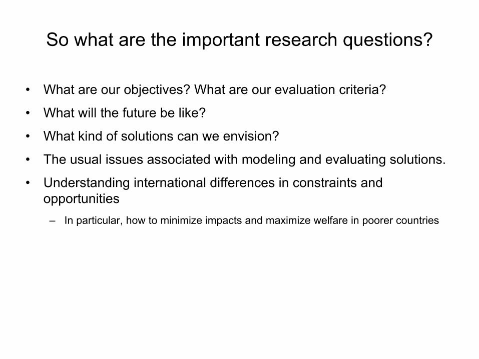
So what are the important research questions?
• What are our objectives? What are our evaluation criteria?
• What will the future be like?
• What kind of solutions can we envision?
• The usual issues associated with modeling and evaluating solutions.
• Understanding international differences in constraints and opportunities
– In particular, how to minimize impacts and maximize welfare in poorer countries
Summary and conclusions
• Dramatic changes in values and technology provide a great opportunity to plan and develop new, sustainable energy, transportation, and land-use systems.
• Electrifying all transport, using the most sustainable primary energy sources (wind, water, and solar power), is the best solution to a wide range of social and environmental problems.
• Our research suggests that electrification probably does not cost (much) more than does a BAU scenario, but provides large benefits. Electrification also appears to have higher net benefits than do biofuels, except perhaps in aviation.

Wait – but what about “practicality,” you say?
This Modern World, Daily Kos, May 16, 2016, http://www.dailykos.com/blog/Tom%20Tomorrow

Well….we did go to the moon...
And more prosaically:
We didn’t get the interstate highway system by putting a tax on horse manure.

All things…Near or far,HiddenlyTo each other linked are,That thou canst not stir a flowerWithout troubling of a star
From ‘The Mistress of Vision’, by Francis Thompson

REFERENCES
Available from me.