transportation research recordonlinepubs.trb.org/onlinepubs/trr/1994/1471/1471.pdf · sponsorship...

TRANSPORTATION RESEARCH

RECORD No. 1471

Highway and Facility Design

Recent Research on Hydraulics and

Hydrology

A peer-reviewed publication of the Transportation Research Board

TRANSPORTATION RESEARCH BOARD NATIONAL RESEARCH COUNCIL

NATIONAL ACADEMY PRESS WASHINGTON, D.C. 1994

Transportation Research Record 1471 ISSN 0361-1981 ISBN 0-309-06104-0 Price: $23.00

Subscriber Category IIA highway and facility design

Printed in the United States of America

Sponsorship of Transportation Research Record 1471

GROUP 2-DESIGN AND CONSTRUCTION OF TRANSPORTATION FACILITIES Chairman: Charles T. Edson, Greenman Pederson, Inc.

General Design Section Chairman: Hayes E. Ross, Jr., Texas A&M University System

Committee on Hydrology, Hydraulics, and Water Quality Chairman: Lawrence J. Harrison, CH2M Hill Secretary: Johnny L. Morris, Federal Highway Administration Steven R. Abt, Jasem M. Alhumoud, Colby V. Ardis, Charles W. Boning, Stanley R. Davis, Charles R. DesJardins; Jeffrey Enyart, David J. Flavell, William H. Hulbert, John Owen Hurd, J. Sterling Jones, Kenneth D. Kerri, Charles A. Mc/ver, Babak Naghavi, Jerome M. Normann, Glenn A. Pickering, Don L. Potter, Richard E. Price, James A. Racin, Everett V. Richardson, Peter N. Smith, Wilbert 0. Thomas, Jr., E. L. Walker, Jr., Ken Young, Michael E. Zeller

Structures Section Chairman: David B. Beal, New York State Department of Transportation

Committee on Culverts and Hydraulic Structures Chairman: A. P. Moser, Utah State University Kenneth J. Boedecker, Jr., Dennis L. Bunke, Bernard E. Butler, Darwin L. Christensen, Jeffrey Enyart, James B. Goddard, James J. Hill, Paige E. Johnson, /raj/. Kaspar, Michael G. Katona, Carl E. Kurt, Bryan E. Little, Timothy J. McGrath, John J. Meyer, John C. Potter, Edward A. Rowe, Jr., James C. Schluter, David C. Thomas, Corwin L. Tracy, Robert P. Walker, Jr.

Transportation Research Board Staff Robert E. Spicher, Director, Technical Activities D. W. Dearasaugh, Engineer of Design Nancy A. Ackerman, Director, Reports and Editorial Services Marianna Rigamer, Oversight Editor

Sponsorship is indicated by a footnote at the end of each paper. The organizational units, officers, and members are as of December 31, 1993.

Transportation Research Record 1471

Contents

Foreword

Multilane Highway Design Crossfall and Drainage Issues A. M. Khan, A. Bacchus, and N. M. Holtz

Correlation of Pavement Surface Texture to Hydraulic Roughness Andrew E. Lewis, Steven B. Chase, and K. Wayne Lee

Hydraulics of Safety End Sections for Highway Culverts Bruce M. McEnroe

Improvements in Curb-Opening and Grate Inlet Efficiency Rollin H. Hotchkiss

Development of Regionalized Curves for Drainage Area Versus Sediment Basin Size Douglass Y. Nichols

Developing Erosion Control Plans for Highway Construction Brian C. Roberts

Flood Analysis in DuPage County Using Hydrological Simulation Program-FORTRAN Model Allen Bradley, Kenneth Potter, Thomas Price, Paula Cooper, Jon Steffen, and Delbert Franz

Small Urban Watershed Use of Hydrologic Procedures Vernon K. Hagen

v

1

10

18

24

31

38

41

47

Urban Hydrology Design Using Soil Conservation Service TR-55 and TR-20 Models Norman Miller and Donald Woodward

Hydrologic Engineering Center Models for Urban Hydrologic Analysis Arlen D. Feldman

Scour Around Wide Piers in Shallow Water Peggy A. Johnson and Eduardo F. Torrico

54

56

66

Foreword

The 11 peer-reviewed papers in this volume were presented at the 1994 TRB Annual Meeting during sessions sponsored by the TRB Committee on Hydrology, Hydraulics, and Water Quality. The first six papers focus on improved drainage and erosion control for highways, and the next five focus on urban drainage design methods.

Kahn et al. report on a research effort to define the relationships among drainage design, vehicle operation, and safety of wide pavements, with particular focus on crossfall and drainage characteristics. Lewis et al. determined the relationships that allow an estimate of the hydraulic roughness coefficient across a pavement to be made through the use of a simple texture measuring technique. McEnroe presents the results from testing of 10 scale models of safety end sections for highway culverts. Hotchkiss reports on laboratory experiments to improve curb-opening and grate inlet efficiencies for specific inlets in Nebraska. Nichols discusses the development of regional charts to provide the required sediment basin size to meet limitations on effluent from construction sites. Roberts presents a recommended procedure for developing erosion control plans for highway construction following basic principles of erosion and sediment control.

Bradley et al. set forth a new approach for handling complex flood design and analysis problems that exist in large urban watersheds through the use of a continuous simulation model, HSPF. Hagen focuses on small urban watersheds and reports on a survey regarding the use of various hydrology procedures for flood analysis. Miller and Woodward discuss two of the urban hydrology procedures mentioned in the paper by Hagen. Both procedures were developed by the Soil Conservation Service. Feldman focuses on new developments and applications for surface water hydrology models developed by the Hydrologic Engineering Center to simulate hydrologic and hydraulic processes in urban areas. Johnson and Torrico assess the complex phenomenon of scour that occurs when the flow depth is shallow relative to a pier width.

v

TRANSPORTATION RESEARCH RECORD 1471

Multilane Highway Design Crossfall and Drainage Issues

A. M. KHAN, A. BACCHUS, AND N. M. HOLTZ

The safety of wet pavements has become a major concern because of the growing need to drain wide pavements. Research on the relationship between drainage design, vehicle operation, and safety, with a particular focus on crossfall and drainage characteristics of wide pavements, is reported. Following an introduction to the subject, the problem of draining wide pavements and the associated safety issues are discussed. The safety implications of longer drainage paths across four or more lanes of high-speed freeway are described in terms of the risk of loss of vehicle control due to skidding or hydroplaning. Models of skidding, hydroplaning, and water depth on pavement are reviewed. Existing practices and potential solutions for effective drainage of wide pavements are discussed. These include the appropriate crossfall design and the effective drainage at the edge of the pavement. A design methodology is advanced for (a) estimating water depth under various conditions at critical locations on highway pavements and shoulders, (b) establishing drain inlet locations, and (c) assessing whether estimated water accumulation can lead to significant loss of control from skidding and hydroplaning. An example application and sample results are discussed. Finally, conclusions on drainage,ge,c:;ign methodology and crossfall standards are presented.

Driving on a highway pavement covered by a layer of water can become unsafe. Even for a highly skilled and alert driver, especially at high speeds, it may become difficult to control the vehicle when a pavement with a layer of water fails to offer the required amount of friction or when a complete separation of tire and pavement occurs-the phenomenon of hydroplaning.

The purpose of the research described here was to investigate crossfall and other pavement surface drainage design features for large multilane freeways from the perspectives of effective drainage and road user safety.

RESEARCH FRAMEWORK

The research approach shown in Figure 1 consisted of the following steps: (a) defining wet pavement safety and drainage issues; (b) study of variables and their conceptual relationships; (c) compiling information on linkages between skid resistance, hydroplaning, and water depth on pavement; ( d) compiling information on models of skid resistance, hydroplaning, water depth, and the highwayvehicle object simulation; ( e) study of design practices. and potential improvements; (f) development of methodology for testing drainage standards and designs; and (h) developing drainage design guidelines.

A. M. Kh.an and N. M. Holtz, Department of Civil and Environmental Engineering, Carleton University, Ottawa, Ontario, Canada KlS 5B6. A. Bacchus, Research and Development Branch, Ministry of Transportation, 1201 Wilson Avenue, Downsview, Ontario, Canada M3M 118.

DRAINAGE AND SAFETY ISSUES

Although research on the tire-pavement interaction has produced a wealth of information on how to improve the skid resistance properties of pavements, vehicle suspensions, brakes, and tire designs, the subject of wet pavement safety continues to be important owing to the increasing widths of pavements to be drained.

At a growing number of urban and suburban sites, because of high travel demand and the necessity to accommodate through traffic as well as collection-distribution functions within a common cross section, freeway pavements have become much wider than when freeways were mainly four lanes. Even under favorable pavement surface and tire conditions, for safety reasons wide highways must be drained effectively through appropriate crossfall and edge-of-pavement drainage designs.

Available literature indicates that poor drainage has been one of the causes for unsafe operations. In Ontario in 1991, 21.8 percent of total accidents occurred under wet pavement conditions (1, p. 26). Analysis of U.S. safety data reported in the literature identified wet surfaces as a probable important contributing factor to accidents, particularly at curves and downgrades (2).

The interactions between automobile tires and the pavement have been investigated by numerous agencies in the past for the purpose of understanding and improving safety. Lack of required skid resistance for safe driving and the onset of hydroplaning are two key phenomena that have been of special interest to researchers around the world. Horizontal forces related to tire-pavement interaction that provide traction, braking, and directional stability were investigated. Because these forces depend on the coefficient of friction between tires and the road surf ace, the means of maintaining a high coefficient of friction to prevent skidding accidents were emphasized. Inadequate drainage of pavement surface is recognized in the literature to be a problem area.

VARIABLES AND LINKAGES

Many factors were identified to be relevant in this research. These are pavement width, crowning considerations, cross slope, longitudinal grade, curvature, superelevation, shoulder arrangement, shoulder surface treatment, water depth, pavement surface characteristics, skid resistance, vehicle operational characteristics (i.e., safe operations and hydroplaning), and cost of .drainage. The linkages between variables were defined initially in a conceptual form, based on the principles of vehicle dynamics, tire-pavement interaction, pavement characteristics, and geometric and drainage designs. As for the cost variable, only qualitative considerations could be addressed because of the scope of the study.

2

Wet Pavement Safety & Drainage Issues

I study of Variables & Their Conceptual Relationships

I Skid Resistance, Hydroplaning & Water Depth on Pavement

I Skid Resistance Hydroplaning Water Depth Models Models Models

I Study of Design Practices

I Modelling Framework & Computer Program Development

I Drainage Design Guidelines

FIGURE 1 Research framework.

HVOSM I studies

MODELS OF SKIDDING, HYDROPLANING, AND WATER ACCUMULATION

The skid number of a pavement is the coefficient of friction multiplied by 100. It is quantified by numerous agencies in accordance with ASTM Test Method E274 (3). The measurements are made by using a test vehicle, including a specified tire for pavement tests. Skidding implies a vehicle motion that results from the driver losing control of the vehicle because of the lack of required tire-pavement friction. If a vehicle is driven faster than the critical speed on wet pavement, the driver can lose control of the vehicle as a result of the onset of skidding. In the normal course of driving, even if excessive speeds are not involved, drivers may react to situations on the highway that may demand more shear force from their tires than is available from the frictional potential between the tire and road (e.g., braking and changing lanes). This may cause the vehicle to skid. Both cars and trucks can skid on wet pavements. In fact, skidding problems are amplified in the case of heavy trucks ( 4).

Safe operation of a vehicle at all speeds and under all types of vehicular movements requires that the available friction (i.e., the maximum friction force that can be generated under the conditions) must exceed friction demand. In the case of wet pavements, available friction drops with increasing speed. The opposite is the case with demand for friction on wet pavements (for directional control or performing the intended maneuvers such as braking, changing lanes, turning, or a combination of these), because it increases with speed (3,5). Although the advent of antilock brake systems has helped to prevent lockup of wheels in emergency braking situations, these observations clearly point to the importance of speed as a major variable in wet pavement safety.

Pavement surface properties are very important in the study of skid resistance on wet pavements. Pavement surface roughness fea-


tures are divided into three scales: roughness, macrotexture, and microtexture. Roughness or unevenness of the pavement primarily affects ride comfort. Macrotexture refers to stone projections (measured by ASTM E 770 method), and microtexture is the harshness of materials (evaluated by PSV by the ASTM D 3319 method). Both macrotexture and microtexture are essential for obtaining an adequate coefficient of friction on wet pavements.

At the tire and pavement contact area, the tire deforms into a flat surface and could trap water. For preventing marked loss of skid resistance, the water trapped in this contact area must be expelled. At higher speeds, large open-flow channels potentially obtainable from the tire tread and the pavement macrotexture are needed because less time is available for expelling water.

However, despite the presence of pavement macrotexture and good tire condition, a thin water film could remain between tire and pavement unless it is expelled by harsh microtexture and a quasidry contact point between pavement and tire is established. Thus, good skid resistance under wet conditions calls for good macro- and microtextures.

Hydroplaning is the phenomenon of the separation of the tire from the road surface by a layer of water. It is recognized that oh a microscopic scale all operational conditions on wet pavements may involve some degree of partial hydroplaning. On a macroscopic scale, hydroplaning occurs only if there is some significant degree of penetration of a water wedge between the tire and pavement contact area ( 6).

Three categories of hydroplaning of pneumatic-tired vehicles have been defined: viscous hydroplaning, dynamic hydroplaning, and tire tread rubber hydroplaning (7).

In the case of light road vehicles, the first two types are relevant to the present study. The third type of hydroplaning occurs only if heavy vehicles such as trucks or aircraft lock their wheels while moving at high speeds on wet pavements exhibiting macrotexture but little microtexture.

On pavements with little microtexture, viscous hydroplaning can occur at any speed in the presence of extremely thin films of water. It is logical to suggest that such a thin film of water remains between tire and pavement because the pavement microtexture required to break it down is absent.

Dynamic hydroplaning occurs when the amount of water encountered by the tire exceeds the combined drainage capacity of the tread pattern and the pavement macrotexture (7). Owing to the impact of tire surface with the stationary fluid, there is sufficient pressure to buckle the tire tread surface inward and upward from the pavement. This causes a progressive penetration (with increased speed) of the fluid film from front to rear of the footprint region of the tire (3,6).

Although the new designs of tires are aimed at improving the drainage capacity of the tread pattern, there is no basis to suggest that dynamic hydroplaning can be prevented.

Past research has resulted in models that can serve as guidelines for the identification of water depth and speed conditions that may lead to dynamic hydroplaning (Table 1) (6,8).

For the estimation of water depth on pavement under various conditions, a search was carried out for suitable empirical and theoretical models. A number of empirical models reported in the literature were examined, and one was selected for further evaluation. This empirical model of parametric form (described later in this paper) was tested against a theoretical model of water flow on pavement (9).

Empirical equations were developed by a number of research groups for estimating the depth of water over the pavement. These research groups were the Road Research Laboratory in the United

Khan et al. 3

TABLE 1 Critical Thickness (mm) of Water Film for Dynamic Hydroplaning

Tire.Condition Speed ('km/h) Good condition Some wear Worn out

80 100 120 130

7.8 5.0 3.5 3.0

4.7 3.0 2.0 1.8

2 .·6 1. 7 1.2 1.0

Source: Calculated from information reported in Reference 6, pp. 11-15.

Kingdom, Yaeger and Miller at Goodyear, and Gallaway et al. at the Texas Transportation Institute (TTI). The research work at TTI was the most comprehensive in terms of the factors studied and the amount of prototype tests and highway field studies carried out. The TTI model was widely tested at great expense in the United States and Europe.

It should be noted that the empirical equations developed by various groups cannot be compared with confidence in terms of their estimates of water depth because the variables incorporated were different. The TTI equation described later in this paper is the only model that is based on all the necessary variables.

The empirical and theoretical models were compared in a number oftest cases. It is recognized that because of numerous assumptions made in the development of the theoretical model, the results of the theoretical model are approximate at best. Despite this limitation, a comparison of the results of two models was favorable. The water depth answers obtained from the empirical model were 20 to 37 percent higher than those obtained from the theoretical model. The conservative nature of the empirical model estimates is considered desirable from the perspective of developing drainage and safety strategies.

The study of safety aspects of factors that could be considered critical in terms of vehicle operation on wet pavement (i.e., those that could result in skidding) called for the use of a computer model. The Highway Vehicle Object Simulation Model (HVOSM) was used for this purpose. This model was developed initially by Cornell University and was refined by CALSPAN of Buffalo, New York, forFHWA.

HVOSM was used for testing vehicle operations for various drainage design, geometric design, and pavement characteristics. The effects of drainage design parameters were studied on turning, lane change, and a combination of these with and without braking. This model is widely used by researchers for determining operating conditions that can lead to loss of control and onset of skidding.

· DESIGN PRACTICES AND SEARCH FOR IMPROVEMENTS

Existing drainage design standards used by numerous transportation agencies date back to the time when freeways were mainly four lanes with only a few six-lane sections. It has been believed by many designers that there is no comprehensive basis in current standards for establishing safe drainage designs for 8- or 10-lane divided highways. Such wide pavements could involve water flow over four or five lanes, and in the absence of well-researched drainage design guidelines, water accumulation may result in safety problems.

Even in the case of six-lane freeways, existing drainage design guidelines are not well defined and cannot be relied on to answer some design questions.

Solutions to wide pavement drainage and safety problems can be found in appropriate crossfall and superelevation design standards, the expedient removal of water at the edge of pavement, and the provision of pavements with good macrotextures as well as rnicrotextures.

It is encouraging to note that skid correction programs are receiving increased attention in Canada, the United States, Europe, and elsewhere around the world. A literature survey indicated that a skid number of 35 is used as the critical skid index. Pavements that show a skid number below 35 are given priority for improvement. Pavements with skid numbers in the range of 35 to 45 are regarded as marginal, and those pavements with skid numbers above 45 are classified as standard (10).

In response to the increasing recognition of the importance of reducing accidents in wet weather, the authorities appear to be keen on the use of adequate superelevation and cross slope, particularly on long-radius curves, and of friction courses (10, 11). Open-graded friction courses (OGFCs) improve friction during wet conditions and reduce splash and spray. However, their less than projected service lives in areas with severe winter climates is a cause for concern. Other friction courses and newer surface treatments offer appropriate texture properties.

DRAINAGE DESIGN METHODOLOGY

Capabilities

This modeling framework, implemented as a microcomputer program called RUNOFF, enables the designer to test drainage design factors in terms of water depth on the pavement, vehicle operating conditions, total amount of water to be drained, and location of drain inlets. From the knowledge of water depth and characteristics of pavement, inferences can be drawn on loss of friction, skidding, and hydroplaning. An additional feature of the model is that it can be used to estimate total water flow and drain inlet spacing.

The model calls for inputs on precipitation, roadway section features, and design decision variables. Computations are carried out for drainage path (i.e., pavement contours), drainage length and slope, and water depth. The estimation of water depth under various conditions and at critical locations on highway pavements and shoulders in conjunction with pavement characteristics enables the analyst to assess whether such accumulation can lead to significant loss of control from skidding or hydroplaning.

4

The methodology assists the designer in testing many. what-if situations without resorting to tedious and time-consuming hand calculations. In tum, the identification of the best design becomes easier.

Model Components

There are three basic components of the model.

• Module A. This part of the model estimates water depth on the pavement.

• Module B. Here, the total quantity of water that is to be drained from a specified section of the roadway is estimated, and the user is advised on factors for drain inlet location decisions.

• Module C. This module is intended to examine the water depth answer obtained from Module A in terms of whether it falls in the satisfactory range. Also, suggestions are offered for changing design parameters or the supplemental skid resistance to be provided.

Module A

The slope of the flow path (in percent) is found from the following expression:

where

S3 = slope of flow path (in percent, expressed in fractional form), S1 = cross slope (in percent, expressed in fractional form), and S2 = longitudinal grade (in percent, expressed in fractional form).

The length of flow path is found as

where Lis the length of the flow path (in m), and Wis the pavement width, measured from the crown line or edge of inside shoulder (in m).

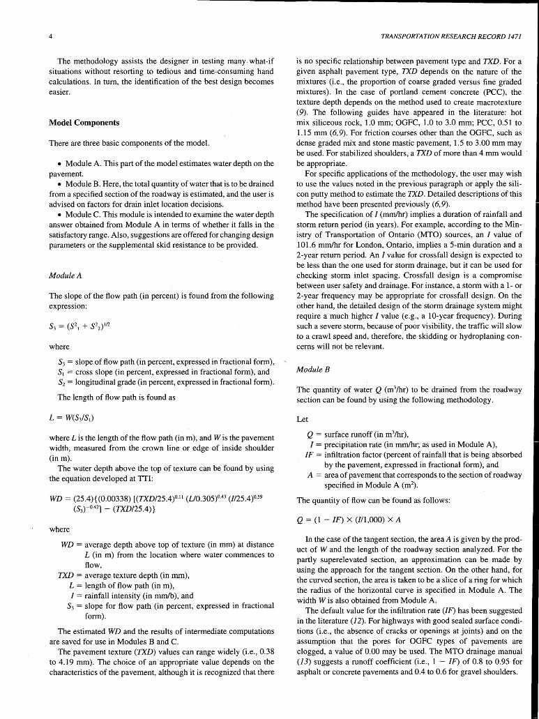
The water depth above the top of texture can be found by using the equation developed at TTI:

WD = (25.4){(0.00338) [(TXD/25.4)0·11 (L/0.305)0.4

3 (//25.4)0·59

(S3)-0.42] - (TXD/25.4)}

where

WD = average depth above top of texture (in mm) at distance L (in m) from the location where water commences to flow,

TXD = average texture depth (in mm), L = length of flow path (in m), I = rainfall intensity (in mm/b ), and

S3 = slope for flow path (in percent, expressed in fractional form).

The estimated WD and the results of intermediate computations are saved for use in Modules B and C.

The pavement texture (TXD) values can range widely (i.e., 0.38 to 4.19 mm). The choice of an appropriate value depends on the characteristics of the pavement, although it is recognized that there


is no specific relationship between pavement type and TXD. For a given asphalt pavement type, TXD depends on the nature of the mixtures (i.e., the proportion of coarse graded versus fine graded mixtures). In the case of portland cement concrete (PCC), the texture depth depends on the method used to create macrotexture (9). The following guides have appeared in the literature: hot mix siliceous rock, 1.0 mm; OGFC, 1.0 to 3.0 mm; PCC, 0.51 to 1.15 mm (6,9). For friction courses other than the OGFC, such as dense graded mix and stone mastic pavement, 1.5 to 3.00 mm may be used. For stabilized shoulders, a TXD of more than 4 mm would be appropriate.

For specific applications of the methodology, the user may wish to use the values noted in the previous paragraph or apply the silicon putty method to estimate the TXD. Detailed descriptions of this method have been presented previously (6,9).

The specification of I (mm/hr) implies a duration of rainfall and storm return period (in years). For example, according to the Ministry of Transportation of Ontario (MTO) sources, an I value of 101.6 mm/hr for London, Ontario, implies a 5-min duration and a 2-year return period. An I value for crossfall design is expected to be less than the one used for storm drainage, but it can be used for checking storm inlet spacing. Crossfall design is a compromise between user safety and drainage. For instance, a storm with a 1- or 2-year frequency may be appropriate for crossfall design. On the other hand, the detailed design of the storm drainage system might require a much higher I value (e.g., a 10-year frequency). During such a severe storm, because of poor visibility, the traffic will slow to a crawl speed and, therefore, the skidding or hydroplaning concerns will not be relevant.

Module B

The quantity of water Q (m3/hr) to be drained from the roadway section can be found by using the following methodology.

Let

Q = surface runoff (in m3/hr), I = precipitation rate (in mm/hr; as used in Module A),

IF = infiltration factor (percent of rainfall that is being absorbed by the pavement, expressed in fractional form), and

A = area of pavement that corresponds to the section of roadway specified in Module A (m2

).

The quantity of flow can be found as follows:

Q = (1 - IF) X (//1,000) X A

In the case of the tangent section, the area A is given by the product of W and the length of the roadway section analyzed. For the partly superelevated section, an approximation can be made by using the approach for the tangent section. On the other hand, for the curved section, the area is taken to be a slice of a ring for which the radius of the horizontal curve is specified in Module A. The width Wis also obtained from Module A.

The default value for the infiltration rate (IF) has been suggested in the literature (12). For highways with good sealed surface conditions (i.e., the absence of cracks or openings at joints) and on the assumption that the pores for OGFC types of pavements are clogged, a value of 0.00 may be used. The MTO drainage manual (13) suggests a runoff coefficient (i.e., 1 - IF) of 0.8 to 0.95 for asphalt or concrete pavements and 0.4 to 0.6 for gravel shoulders.

Khan eta!.

This methodology is not intended for use in the development of drainage designs in terms of suggesting gutter designs (if applicable), selecting inlet grates, and establishing the locations of drain inlets, and so forth. However, it supplies the designer with preliminary information on the spacing of drain inlets.

The inlet spacing calculations take into account the amount of water to be drained, the gutter capacity, and the design spread. The design spread is the distance along the paved shoulder or roadway cross section that will be flooded. This variable in turn affects gutter capacity, the depth of flow along the gutter, and thus the capture rate of the inlet (13).

For wide pavements on freeways, the likely presence of a shoulder will not result in flooding of the traveled way. According to the MTO design manual, for freeways· a maximum design spread of 1.5 m is allowed, provided that the gutter is at the outer edge of a paved shoulder. Also, the MTO drainage manual provides guidelines for increasing design spread under specified conditions.

From charts contained in the MTO drainage manual (13), for selected inlet grate, gutter grade, and design spread, a gutter flow capacity (Q8 ) can be found. On the assumption that the local runoff (Q,) to be conveyed is equal to Q8 , then the inlet spacing can be found from the following formula: ·

!NL= (3.6 X 106 X Q,)l[W XIX (1 -·IF)]

where

!NL = length of roadway section to be drained (first inlet assumption) (in m),

Q, = runoff (set equal to Q8 ) (in m3/sec), W = width of pavement (and shoulder if applicable) to be

drained (in m), I = rainfall intensity (in mm/hr),

IF= infiltration rate (expressed in fractional form), and 1 - IF = runoff coefficient.

1. In this part of the methodology, the Q (in m3/hr) calculated earlier is converted to Q (in m3/sec): Q (in m3/sec) = [Q (in m3/hr) found for the road section]/(3,600).

2. Next, the analyst is advised to compare this magnitude of water with what can be drained by the gutter at capacity and the spacing of inlets equal to a maximum of 150 m (specified by MTO). The methodology asks the user to specify Q8 • For example, for inlet grate DD-713-B, a gutter grade of 4 percent, and a design spread of 1.5 m, Chart E4.74A in the MTO drainage manual (13) indicates that Q8 equals 0.045 m3/sec.

3. Compare Q8 with the demand flow rate. If Q8 is greater than the demand flow rate, one inlet is required. It can be located within this section unless an adjoining road section is available. If Q8 is equal to the demand flow rate, one inlet is required within this section. If Q8 is less than the demand flow rate, more than one drain inlet is required. Inlets can be located according to the standard procedure of MTO. In all these cases, use Q8 to calculate !NL. If !NL is greater than 150 m, set it equal to 150 m, its .maximum value specified by MTO; if not, use the calculated INL, as follows:

!NL required= (3.6 X 106 X Q,)l[W XIX (1 - IF)]

The user should specify the Q8 value. If not use a default value for Q, equal to Q8 equal to 0.045 m3/sec.

4. The user of the methodology is advised to refer to the MTO drainage manual (13) for developing a detailed design for pavement drainage.

5

Module C

1. Check the water depth against the guidelines presented in Table 2. A check should be made against the critical WD value that could result in skidding or hydroplaning. The user should be advised to check skid resistance and upgrade it if necessary.

2. The design could be modified, and the procedure could be repeatedto calculate a new value for WD and check skid resistance deficiency and hydroplaning potential.

3. Following a testing of all design changes (e.g., crossfall) that could be made, the designer must explore means to enhance skid resistance. Guidelines are provided by the methodology, including the improvement of surface texture by adding a layer of OGFC or other new surf ace treatments, and speed control.

Example Application

Assume that a freeway pavement section (of 100 min length) of four lanes is expected to drain toward the outside shoulder. The dimensions for the lanes and cross slopes are presented later. Information on the outside shoulder is not provided. Given that I is equal to 101.6 mm/hr and TXD is equal to 2.5 mm, find WD at the edges of the lanes (i.e., Points A, B, C, and D). The results are presented . in Table 3.

Sample Calculation

Module A Find WD at Point A for TXD = 2.5 mm, L = W = 3.7 m, I= 101.6 mm, S1 = 0.02, S2 = 0, and S3 = [(0.02)2] 112 = 0.02. WD = -0.22 mm (i.e., below the top of pavement texture).

Module B Length of section = 100 m, width of section = 14.8 m, A =area to be drained= 1,460 m2

, and I= 101.6 mm/hr. For IF = 0.0, Q = 150.36 m3/hr, and for IF = 0.4, Q = 90.22 m3/hr. For demand Q = 150.36 m3/hr, Q/sec = 0.042 m3/sec. Ask the user to specify Q8 ; if it is not specified, use the default value. Q8 of 0.045 > Q demand; one inlet will be sufficient:

!NL= [(3.6 x 106 x 0.045)]/[(14.8 x 101.6 X (1 - 0)] = 107.7 m

Since it is less than the maximum value of 150 m, use 107.7 m. If there is an adjoining section of the roadway, the drain inlet could be located there. If not, locate the inlet in this section.

Module C Compare WD with the values provided in Table 2. The results are generally acceptable, but check skid characteristics; also, repeat the design with a higher value of cross slope and attempt to reduce WD to approximately 1.0 mm if possible.

SAMPLE RESULTS

The use of the methodology described here and the HVOSM computer simulations have resulted in (a) water depth estimates on pavement and shoulder surfaces for a large number of combinations of crossfall, longitudinal slope, roadway width, pavement texture, superelevation for curved sections, and rainfall intensity; (b) water

TABLE 2 Water Depth and Assessment of Design

WD (mm)

0-1

1-2

2-3

>3

Assessment•

Acceptable

Acceptable but check skid characteristics; vehicles with worn out tires may hydroplane; potential for viscous hydroplaninq

Acceptable but check skid resistance; vehicles with some tire wear may hydroplane; potential for dynamic hydroplaninq

Not recommended-hydroplaning potential

Action Required ---------------------------No action required

Repeat design, reduce WD if possible; if not, no action needed for friction course surfaces; check skid resistance for other surf aces and take actions such as signaqe, improved texture for asphalt pavement & tiµing for concrete pavement.

Repeat desiqn, reduce WD if possible; if not, use signaqe; no other action needed for friction courses with qood skid resistance; improve texture for other bituminous surfaces; improve friction for concrete pavement.

Repeat desiqn, reduce WD if possible; if not, use siqnage & check skid resistance of all pavement types; use all feasible actions (e.g., friction courses) to improve skid resistance and reduce hydroplaning potential.

• Based on information contained in Table 1.

TABLE 3 Results of Sample Application

Lane Lane 1 (Inside lane)

Inputs

Lane 2 ·Lane 3 Lane 4 (Outside lane)

Width 3.7m 3.7m 3.7m 3.7m

Crossfall

Reference Point

2% --> 2% --> 2% --> 2% -->

A B C D

-----------------------------------------------------------------WD (mm) Q (cub.m/h) IF=O.O IF=0.4

-0.22

37.59 22.56

0.55

74.17 44.50

1.14

111.78 67.67

1.61

150.36 90.22

Khan et al.

depth estimates for test cases involving variable cross slopes for different parts of the roadway cross section; and ( c) estimation of speed at impending skid for a large number of combinations of crossfall and superelevation, radius of curvature, rollover, longitudinal slope, pavement skid number, and relevant vehicle maneuvers (i.e., driving with and without brake action, turning, and changing lanes).

Figure 2 shows sample results in terms of water depth. In Figure 2 the longitudinal slope is assumed to be 0 percent. For reasons noted in the next section, results are almost identical even if a longitudinal slope is involved. Sample results obtained from the HVOSM applications shown in Figure 3 indicate estimates of driving speeds at impending skid. The sample results clearly show the need for adequate skid numbers and to avoid high rollover (R.0.) effects. Sample results presented in Figure 4 illustrate the influence of low skid numbers and brake action for 0 percent grade ( G = 0 percent) and 3 percent grade.

Crossfalls for freeway pavements are presented in Table 4 for two pavement texture values and representative precipitation conditions. Also shown is the percent rollover that corresponds to crossfall and speed at impending skid for a pavement with a skid number of 40. As the footnote to Table 4 indicates, a skid number of 40 represents a marginal skid resistance. Logically, for increasing pavement width, the crossfall must be increased to limit the

Water depth above top of texture (mm) 3~~~~~~~~~~~~~~~~~~~~~~-,

2.5

1.5

0.5

1.5 2 2.5 3 3.5 4 4.5

Crossfall (%)

SO=Oo/o,lm101.6mm/h,TXD=2.5mm

FIGURE 2 Water depth for S2 equal to 0 percent.

1 ~ 0 w w a.. en

SKID NO.(SN)

FIGURE 3 Lane change on tangent.

5

---R.0.:10% --R.0.:8% --R.0.:6%

~

R.0.:4% --R.0.:3%

~ ~ 0 w w a.. en

OF ROAD(R:1350M,BRAKE FOR G--0% & G=-3%)

10 20 30 40 50 60

SKID NO. (SN)

-BRAKE

FIGURE 4 Driving on superelevated part of road (R = 1350 m, brake for G = 0 percent and G = -3 percent).

7

water depth to a specified level. As expected, higher rollover values result in decreasing speeds for safe skid-free driving. For higher rainfall intensities or a decrease in pavement texture, crossfalls must be increased to limit water depths to acceptable values, and as a consequence the increasing rollover will reduce speeds at impending skid. As shown in Table 4, an increase in TXD will result in effects that would be opposite those of a decrease in TXD.

Analyses were carried out to estimate water depth and speed at impending skid for five lanes with a superelevation of 6 percent. The results shown in Table 5 indicate that without brake action the speed at impending skid is satisfactory, and even with brake action the skid-free operating speed is reasonably high.

CONCLUSIONS

Many conclusions were drawn from the results achieved in the present study (14). Because of space limitations only the highlights are presented here.

1. Studies of surface drainage and vehicle simulation indicate that drainage of the pavement (i.e., crossfall and superelevation as well as effective edge of pavement drainage) is a very important consideration in cross-section design. Also, the importance of reducing water thickness on pavement is stressed because it has a critical influence on the friction available at the tire-surface interface, and thus the safe operation of the vehicle.

2. Both pavement surface water depth and vehicle speed are considered critical elements for hydroplaning.

3. Better geometrics (e.g., higher radius of curvature, adherence to design superelevation rates, and use of spiral transition curves) and pavements of high-quality macrotexture and microtexture improve the safe skid-free driving speed.

4. A water layer of 1.0 to 1.5 mm can be regarded as acceptable from the vehicle operation perspective. However, design modifications are advisable for higher values. It will be necessary to have high pavement skid resistances, should the pavement be subjected to higher water depths.

· 5. Crossfall and pavement width are the two most important variables for reducing water depth. Although the longitudinal slope increases the length of the flow path, it also has the opposite effect on water depth because it enables faster drainage owing to an

8 TRANSPORTATION RESEARCH RECORD 1471

TABLE 4 Crossfall for Freeway Pavements(/= 101.6 mm/hr)

Maximum No. Of crossf all for Rollover &. Speed at Lanes Draining Water Depth Impending Skid at SN=4o• in the Same -------------- -------------------------------Direction J:.5 mm 1.00 mm Boll over s:eeed Rollover s:eeed ------------- (%) (%) (%) (Km/h) (%) (Km/h) Pavement TXD=2.5mm 2 lanes 1.5 2.0 3 158 4.0 140 3 lanes 2.0 2.5 4 140 5.0 127 4 lanes 2.5 3.0 5 127 6.0 119 5 lanes 3.0 4.0 6 119 8.0 99

Pavement TXD=3.0mm 2 lanes 1.0 1.5 2 175 3.0 158 3 lanes 1.5 2.0 3 15·9 4.0 140 4 lanes 2.0 2.5 4 140 5.0 127 5 lanes 2.5 3.0 5 127 6.0 119

Note: The range of skid numbers (SN) 35-45 is regarded "marginal". SN 35 is considered as the critical skid number.

• Without brake action.

TABLE 5 Evaluation of Superelevation Rate

6% Superelevation, Radius of curvature 1350 m; Design Speed 160 km/h; 0% Longitudinal Grade -----------------~------------------------------------------·

Water Depth for 5 Lanes Draining in the Same Direction

Speed At Impending Skid At SN=40

with Braking Without Braking

Less than 1 mm 106 km/h 159 km/h

Note: I= 101.6 mm/h, TXD = 2.5 mm

increase in the slope of flow path. The net result of the presence of longitudinal slope is that there is only a small change (an increase) in water depth.

6. Crossfalls for freeway· pavements, shown in Table 4 for representative precipitation and pavement texture conditions (e.g., 2.5 mm), suggest that values below 2 percent should be avoided for wide pavements. For a texture of 2.5 mm and a rainfall intensity of 101.6 mm/hr, up to five lanes with a crossfall of 3 percent can be drained in the same direction without exceeding a water depth of 1.5 mm. Increasing the crossfall to 4 percent would limit the water depth to 1 mm. The rollover and speed at impending skid at a skid number of 40 appear to be reasonable.

7. Wide pavements with long radii of curvature can be subjected to a high-thickness water layer unless they are designed with superelevations that match or exceed the tangent crossfall shown in Table 4. A 6 percent superelevation would be sufficient to keep the water layer at the edge of a 20-m roadway (five lanes plus a partially paved shoulder) to less than a 1-mm layer depth (Table 5).

ACKNOWLEDGMENTS

This paper is based on a study sponsored by the Ministry of Transportation, Ontario.

REFERENCES

1. Ontario Road Safety Annual Report 1991, Ministry of Transportation, Downsview, Ontario, Canada, 1991.

2. Dunlap, D. F., P. S. Fancier, Jr., R. S. Scott, C. C. MacAdam, L. Segel, et al. Influence of Combined Highway Grade and Horizontal Alignment on Skidding. Final Report UM-HSRl-PF-74-1 Vol 2. NCHRP, TRB, National Research Council, Washington, D.C., Sept. 1974.

3. Hegmon, R.R. Tire Pavement Interaction. Proc., International Congress and Exposition, Office of Research, Development and Technology, FHW A. SAE, W arrendale, Pa., 1987. Paper 870241 in SAE Technical Paper Series.

4. Jackson, L. E. Vehicle-Environment Compatibility with Emphasis on Accidents Involving Trucks. Proc., Vehicle Highway Infrastructure:

Khan etal.

Safety Compatibility. SAE, International Congress and Exposition, SAE, Detroit, Mich., 1987.

5. Zuieback, J. M. Methodology for Establishing Frictional Requirements. In Transportation Research Record 623, TRB, National Research Council, Washington, D.C., 1976, pp. 51-61.

6. Gallaway, B. M., et al. Tentative Pavement and Geometric Design Criteria for Minimizing Hydroplaning. Texas Transportation Institute, Texas A&M University, Report FHWA-RD-75-11. FHWA, U.S. Department of Transportation, Feb. 1975.

7. Browne, A. L. A Mathematical Analysis for Pneumatic Tire Hydroplaning. Presented at ASTM Winter Meeting, 1973.

8. Gengenbach, W. The Effect of Wet Pavement on the Performance of Automobile Tires. Universitiit Karlsruhe, Karlsruhe, Germany. (Translated by CALSPAN, Buffalo, N.Y., July 1967.)

9. Gallaway, B. M., D. L. Ivey, G. Hayes, W. B. Ledbetter, R. M. Olson, D. L. Woods, and R. F. Schiller, Jr. Pavement and Geometric Design Criteria for Minimizing Hydroplaning. Texas Transportation Institute, Texas A&M University, Report FHWA-RD-79-31. FNWA, U.S. Department of Transportation, Dec. 1979.

9

10. Conti, T. C., et al. Maintenance Skid Correction Program in Utah. Presented at 72nd Annual Meeting of the Transportation Research Board, Washington, D.C., 1993.

11. A Policy on Geometric Design of Highways and Streets. AASHTO, Washington, D.C., 1990.

12. Carpenter, S. H. Highway Subdrainage Design by Microcomputer: (DAMP) Drainage Analysis & Modelling Programs, Version 1.1. Department of Ci vii Engineering, University of Illinois, Report FHW AIP-90-012. FHW A, U.S. Department of Transportation, Aug. 1990.

13. Drainage Manual, Vol. 2, Ministry of Transportation, Downsview, Ontario, Canada, 1984.

14. Khan, A. M., N. M. Holtz, and Z. Yicheng. Design Cross/all and Drainage Issues. Ministry of Transportation, Downsview, Ontario, Canada, March 1993.

The opinions expressed in this paper are those of the authors.

Publication of this paper sponsored by Committee on Hydrology, Hydraulics, and Water Quality.


Correlation of Pavement Surface Texture to Hydraulic Roughness

ANDREW E. LEWIS, STEVEN B. CHASE, AND K. WAYNE LEE

A study was performed to determine whether a correlation exists between the pavement's texture parameters, as determined by the outflow meter, texture beam, sand patch, and texture van, and the hydraulic roughness of the same pavement as measured by Manning's n-value. Because of an ever-changing texture from weathering and traffic, it is not practical to test for hydraulic roughness in the field. Therefore, the project incorporated the use of a laboratory hydraulic flume to perform flow tests on 10 different pavement types found in the field. Because wet pavements are a cause of many highway accidents as a result of hydroplaning, a correlation between surface texture and hydraulic roughness will help an engineer to determine whether a hydroplaning problem exists for a given rainfall intensity. From testing it was found that relationships exist between the texture and hydraulic roughness. It was also found that the outflow meter results were inversely related to pavement texture. With this information the engineer can use a simple texture-measuring technique to estimate the hydraulic roughness coefficient.

The purpose of the study described here was to determine whether a correlation exists between· the pavement's surface texture parameters and hydraulic roughness. The surface texture was measured by the FHW A outflow meter, sand patch method, texture van, texture beam, and British pendulum methods. Pavement specimens were then tested in a flume to determine hydraulic roughness coefficients, Manning's n-values.

Hydroplaning is a phenomenon in which automobiles lose control by skimming the surface of wet roads because of the presence of a thin layer of water between the tire and the pavement. Because hydroplaning is a function of hydraulic roughness, a method is needed to determine Manning's n-value. Because of the everchanging surface texture from weathering and traffic, it is not practical to test for hydraulic roughness in the field. Therefore, by correlating hydraulic roughness determined in the laboratory to pavement texture, which can be readily determined in the field, the engineer can quickly estimate the pavement's hydraulic roughness in the field, and thus hydraulic roughness can be periodically monitored for safety.

To achieve the goals of the study, the following objectives were accomplished:

1. A comprehensive literature review of hydroplaning, skid resistance measurement, pavement texture measurements, pavement hydraulics, and other related topics.

2. Replicating pavement textures in the hydraulic flume at Turner Fairbank Highway Research Center (TFHRC) and conduct-

A. E. Lewis, Pavement Consultancy Services, A Division of Law Engineering, 12104 Indian Creek Court, Suite A, Beltsville, Md. 20705-1242. S. B. Chase, FHWA, 6300 Georgetown Pike, McLean, Va. 22101-2296. K. W. Lee, Department of Civil Engineering, University of Rhode Island, Kingston, R.I. 02881.

ing flow tests in the laboratory to determine Manning's n-values for the pavements.

3. Obtaining field texture measurements and skid resistance measurements for similar pavement sections.

4. Data analysis to determine whether a correlation between the texture measurements and Manning's n-value exists.

SIGNIFICANCE OF SURFACE TEXTURE

Wet pavement is a major cause of highway accidents. It induces hydroplaning, reduces skid resistance, and affects vehicle control. If proper surface characteristics of the pavement are constructed and maintained on the roadway, these hazards to vehicle travel can be greatly reduced.

Roadway textures can be obtained through the design of the pavement mixtures, size and grading of the aggregates, construction procedures, or surface finishing methods or by grooving and etching existing pavements. Texture is considered to include the structure and porosity of the top layer, as well as the aggregate's individual properties of mineralogy, shape, and gradation (1).

The term surface texture has been used to describe qualitatively and quantitatively the appearance and feel of a pavement surface. The qualitative influence of pavement surface properties, namely, microtexture and macrotexture, on the tire-pavement skid resistance has been known for years. Recently, there has been an interest in quantifying this influence (2).

Interest in developing methods for measuring pavement texture has stemmed from the theory that the surface texture is related to the skid resistance of a tire pavement combination during braking, cornering, or acceleration of the vehicle. In a study by Moore (3) a surface texture laboratory was created to investigate surface roughness. The results from laboratory tests were compared with those obtained from any of the following three sources:

1. An instrumented vehicle performing specified maneuvers, 2. A test wheel loaded against and driven by a steel drum, or 3. A simplified laboratory model to simulate the interaction

between tire and pavement.

For Moore's study the texture laboratory consisted of a flow meter (to assess the relative drainage abilities of selected pavements), a profile-measuring device (to verify the predictions afforded by the outflow meter), a draping apparatus (to simulate the draping zone), a sinkage model (that duplicates the squeeze-film action in the sinkage zone), and a British portable skid resistance tester for general laboratory use.

Harwood et al. (2), along with the already mentioned test methods, used a sand patch test. The sand patch test procedure can be

Lewis etal.

found from the guidelines of the American Concrete Paving Association (4). Additional texture measurement procedures include the grease patch, putty impressions, profilograph, texture meter, and a surf indicator. These test procedures are described in detail in works by Rose et al. (5), Hegmon and Mizoguchi (6), Rose et al. (7), Dahir and Lentz (8), Henry and Hegmon (9), and many others.

TEXTURE ANALYSIS

Efforts to understand and quantify the texture effects in tirepavement interactions have been limited. This is a result of difficulties encountered in the experimentation or theory to determine many individual contact points between the tire and the pavement. Research has been performed to develop a method to predict the normal contact forces that are created from the surface texture (10). To demonstrate the usefulness of this method, texture-induced con~ tact pressure and length information are computed. Contact pressure is used to analyze individual peak pressures and to construct force time histories that excite tire models for predicting vibrational response and rolling resistance. Contact length is used to approximate tire envelopment into the surface texture. This is beneficial, because information pertaining to skid resistance parameters such as void area and depth of penetration is incorporated into the analysis (11). These detailed computational algorithms can be coupled with approximations from this project to understand and predict the factors influenced by surface texture such as skid resistance, rolling resistance, and vehicle performance.

Skid Resistance

. With higher-speed traffic and increasing volumes, the numbers of accidents tend to increase. Under such conditions vehicle control and maneuverability rely heavily on the friction between the tire and the pavement to avoid an accident. Water on the roadway is a major factor in highway accidents. It induces hydroplaning, reduces skid resistance, and adversely affects vehicle control.

Skid resistance is a general term used to describe the level of friction between a roadway surface and the vehicle's tire. On wet paveme~lts speed is the most significant parameter, because the skid resistance at the tire-pavement interface decreases with increases in speed. The tire-pavement skid resistance can be measured in several testing modes: locked-wheel braking, brake slip, drive slip, and cornering slip. However, the locked-wheel method has gained the widest acceptance for skid resistance testing throughout the United States (2). The most common measurement of the locked-wheel method is the skid number (SN), which is defined as 100 times the coefficient of friction determined by a locked-wheel test. ASTM has standardized this procedure, and testing is accomplished by a two-wheel trailer towed by a truck at a constant speed of 40 mph. Water is sprayed at a standard thickness of 0.002 in. by nozzles located in front of the trailer's wheels. This requires a flow rate of 4.0 gal/min/in. of wetted width. The trailer's brakes are activated on one or both wheels. By using a standardized tire, wheel torque can be interpreted to obtain frictional force and the resulting SN.

Because periodic testing is conducted on all state highways, SNs are ·widely available from most states. Despite its availability, the SN is only one of many parameters needed to design safe roadways. Since the skid test is standardized to one type of tire and one depth of water, other parameters that incorporate a wider range of data

11

need to be developed. For example, two pavements can have similar SNs at 40 mph but can have very different SNs at higher speeds. Therefore, use of data from the skid test as well as other test procedures provides a better understanding of hydroplaning and skidding and could help to increase safety.

Hydroplaning

Total (full dynamic) hydroplaning is a phenomenon in which a tire is completely separated from the pavement by a fluid layer and the . friction at the tire-pavement interface is nearly zero. Hydroplaning is caused by the buildup of fluid pressures within the tire-pavement contact zone. When the total uplift resulting from hydrodynamic pressures exceeds the downward force (vertical load), the tire moves upward to maintain the dynamic equilibrium of the forces. During hydroplaning a gust of wind, a change in road superelevation, or a slight tum can create an unpredictable and uncontrollable sliding of the vehicle (12).

EXPERIMENTAL DESIGN AND PROGRAM

Objective

The objective of the present study was to develop a correlation between pavement surface texture and hydraulic roughness as quantified by Manning's n-value. This was accomplished by

1. Using various test methods to measure surface texture, ·2. Designing and building a flume to measure Manning's

n-value, and 3. Collecting field data for comparisons .

The reasons for using several methods to measure surface texture were to compare each method to find the best correlation and because not all methods are available to everyone. The methods used to measure surface texture in the present study were

· 1. British pendulum (ASTM E303) (9), 2. Skid trailer (ASTM E274) (7), 3. Texture van (Pennsylvania State University and FHW A), 4. Texture beam (FHW A) (9), 5. Outflow meter (FHW A) (6), and 6. Sand patch (ASTM E965) (6).

Summary of Test Methods

The British pendulum tester is a dynamic pendulum impact-type tester used to measure the energy loss when a rubber slider edge scrapes over a test surface. This method measures the frictional property associated with the microtexture of the surface. It may also be used to determine the wearing or polishing properties of pavement surface materials. For this test method the pavement surface is cleaned and thoroughly wetted before testing. The pendulum slider is positioned to come barely into contact with the test surface. The pendulum is raised to a locked position and is then released, thus allowing the slider to make contact with the test surface. A drag pointer indicates the British pendulum number (BPN). The greater the friction between the slider and the test surface the more retarded the pendulum's swing, thus recording a larger BPN.

12

The skid trailer measures the skid resistance of paved surfaces with a specified full-scale automotive tire. This measurement represents the steady-state friction force on a locked test wheel as it is dragged over a wetted pavement surface under constant load and at a constant speed. The wheel's major plane is parallel to its direction of motion and perpendicular to the pavement. The skid resistance of the paved surface is determined from the resulting force or torque . record and is reported as the SN described earlier.

However, skid resistance is primarily a function of pavement microtexture. Therefore, a correlation between skid resistance and pavement macrotexture was not successfully determined. Further details can be found in the section on test results.

The texture van is an automated device developed jointly by FHWA and Pennsylvania State University. The texture van incorporates the use of a strobe light and camera. The flashing strobe light produces shadows that the camera then photographs as an image of the pavement texture. The image is then separated into light and shadow regions, which are digitized into a computer. The area of light is then calculated and converted into a root mean square value for pavement surface height. The texture van can be operated at various speeds, allowing for a safer testing environment because the texture van can stay with the traffic flow.

The texture beam determines the texture height of test samples in the laboratory and the field. The apparatus consists of a hinged arm with a needle that drags along the surface at constant speed. A linear variable differential transducer attached to a data acquisition system records voltage differences as the needle pivots up and down along the pavement surface. The texture beam test method was developed at TFHRC.

The sand patch method is a procedure for determining the average depth of pavement surface macrotexture by applying a known volume of material (glass beads) onto the surface and measuring the total area covered. The sand patch method is not significantly affected by the surface microtexture.

The outflow meter is a device that measures the drainage characteristics of a pavement surface. A column is filled with water and placed on a clean surface. The bottom of the outflow meter has a rubber gasket that contacts the pavement surface~ A stopper is removed and a timer is started, which determines how long it takes for the water to drop 2 in. The water flows through the contact zone between the rubber gasket and pavement surface. The timer is stopped when the water level falls in the outflow meter's column by 2 in. For the present study the outflow meter data are correlated to surface texture and a regression equation is developed.

Flume Design

To determine Manning's hydraulic roughness coefficient n, a flume was designed and constructed. The flume's specifications were as follows:

• Size: 20 ft long and 28 in. wide, _ • Slope: 0.5 in. over 20 ft = 0.002 ft/ft, • Water Depth: 1.0 in. (approximate), and • Flow: varied and measured by (a) paddle wheel flow meter and

(b) 90-degree V-notch weir box.

To ensure the correct slope, the flume was surveyed twice and shimmed to the correct dimensions. The water entered the flume by flowing into a head box. The head box provided an equal distribu-


tion of water over the entire width of the flume. Several fins were added to the head box to eliminate waves and turbulence that could enter the system. The paddle wheel flow meter was placed in the piping system just before the head box. The flow meter determined the amount of water entering the system. The V-notch weir box was placed at the end of the flume system to collect the exiting water, which enabled comparison with the flow meter. This ensured that the flow entering the system was equal to the flow exiting the system. This dual method of flow measurement was chosen because small amounts of water loss occurred through the seams created at the head box and the V-notch weir connections. The flume was designed so that the sides, head box, and V-notch weir box could easily be removed to change the pavement types that were to be tested. Therefore, careful monitoring was required to minimize leaks.

Pavement Types

Ten pavement types were tested in the project described here. The types of textures chosen were similar to those found in the field. The following types of pavement surfaces were investigated:

• Smooth trowel finish portland cement concrete (PCC); • Broom finish PCC; • Tinned finish PCC with 3/s-in. pea stone; • Tinned finish PCC without pea stone; • Tinned finish vertical PCC; • Tinned finish shallow PCC without pea stone; • Asphalt concrete (AC), Virginia Specification SM2A, rough; • AC, Virginia Specification SM2A, smooth; • Epoxy-treated wearing surface, sand; and • Epoxy-treated wearing surface, crushed stone.

These surfaces were also chosen to present a wide representation of texture to better correlate to Manning's n-value. Tinned surface consists of 1/2-in. spaced grooves that are l/s-in wide and approximately 1/4-in. deep. The tinned vertical surface means that the surface was grooved perpendicular to the flow of water. All other tinned surfaces were grooved parallel to water flow. It must be remembered that the length of the flume represents the cross section of the lane. Therefore, if the lane is cross sloped, tinning parallel to water flow is perpendicular to the vehicle travel direction.

Because of the time constraint, open-graded friction courses were not available for testing. Therefore, a standard SM2A mixture was used with a low compaction effort to find the effects of a porous surface texture on Manning's n-value. The epoxy-treated surfaces represent two common aggregate sizes used in the Virginia area for epoxy-treated bridge deck surfaces.

Test Plan

After placing the pavement in the flume, the walls, head box, and V-notch weir box were inserted. With the use of a variable-speed pump, flow was adjusted so that a depth of approximately 1 in. was maintained along the length of the flume. Flow was maintained for about one hr to allow for steady-state flow. Using three point gauges attached to a movable pridge, the water depth was recorded at 2-ft intervals. One of the point gauges was placed at the center and one on each side 5 in. in from the walls. The system with three point

Lewis et al.

70

• 65

~ • • • z· I e 60 • • z E • :J 55· z

"O :.;: • (/)

50 • • • •

46+-~-.-~....,..~-.-~--.....-~~~T'"-'~....-~---~-,-~~

100 150 200 250 ~ 350 400 450 500 550 600 Outflow Meter (1/100 eec)

FIGURE 1 Skid resistance versus outflow meter reading in Rhode Island.

~ z e z E :I z 32 .ii: (/)

60

55

50

45

40

35

30 0.6

• • •

0.7

•

0.6 0.9

• •

• •

Sand Patch (mm)

•

•

•

1.1

• ••

1.2

FIGURE 2 Skid number versus texture height in Washington, D.C.

gauges allowed for measurements to be made across the flume to determine whether the flow was uniform as well as laminar. Readings were taken from the flow meter and V-notch weir to determine the flow (Q) in the system. By applying Manning's equation, hydraulic roughness was determined.

Texture tests were then taken at 4-ft intervals in the center of the test flume. The head box, walls, and V-notch weir were then removed. The pavement was broken into test sections and taken for further laboratory tests. The flume was then prepared for another test pavement.

Field Study

Initially, the project concentrated on finding a relationship between skid resistance and Manning's n-value. Field tests with the skid trailer were performed along with pavement texture tests in Rhode Island, Virginia, and Washington, D.C. From investigation of these findings, no direct correlation existed between skid resistance and pavement texture. The focus of the study was then changed to determine whether a relationship existed between pavement texture and Manning's n-value. Skid testing continued in the laboratory as a secondary objective to determine whether there is any relationship between hydraulic roughness and skid resistance. Because skid resistance data are widely available, it would be helpful to find a

13

correlation to Manning's n-value to determine the hydroplaning characteristics of the pavements' surface.'

TEST RESULTS AND ANALYSIS

Initial test results were compared to explore the relationship between skid resistance and pavement texture. Test results obtained by using the ASTM skid trailer in Rhode Island, Washington, D.C., and Virginia are shown in Figures 1 to 3, respectively. It was observed that no direct correlation can be established .

Linear regression analysis was performed on the skid data corre-. lation to texture, and it was determined to be a poor correlation. The

poor correlation may be due to the inaccuracy of positioning of the texture test with the skid patch. Also, pavement macrotexture does not significantly affect skid resistance. Therefore, it was concluded that a linear relationship between SNs and texture did not exist.

Poor correlations were also found in previous studies involving skid resistance and its relationship to texture. In a study by Dahir and Lentz (8), no fixed correlation of texture depths with SNs as measured with the skid test trailer at 40 mph was evident, as shown in Figure 4.

1.1

•

0.9

{!! 0.8· • :::J

1 • 0.7 •• • • • ~ • I• 0.6. • '* • ••

• • • • • 0.5 • • • ··~ • • ... 0.4

38 40 42 44 46 48 50 52 54 Skid Number (SN40)

• Texture Van • Texture Beam • Sand Patch

FIGURE3 Skid number versus texture at TFHRC, McLean, Va.

SN40 w Sand Pa1ch (mm) 75

• • 70 • •

~ ii • • z 65 • • e • z • ••

60 • • E •• • :::J • • z • • "O 55 • • :.;: •

(/)

50 • •

45 1:2 1.4 1.6 1.6 0 0.2 0.4 0.6 0.6

Texture Height (mm)

FIGURE4 SN versus texture (8).


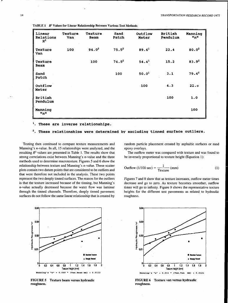
TABLE 1 R2 Values for Linear Relationship Between Various Test Methods

Linear Texture Texture Sand Outflow British Manning Relations Van Beam Patch Meter Pendulum "n"

Rz

Texture 100 94. oz 75. 5Z 89. 61 22.4 so.oz Van

Texture 100 74. 5Z 54. 41 15.2 83 .9z Beam

Sand 100 so. 01 3.1 79 .4z Patch

Outflow 100 4.3 2~. ::> Meter

British 100 1.0 Pendulum

Manning 100 "n"

1 These are inverse relationships. . z These relationships were determined bv excludinq tinned surface outliers. .

Testing then continued to compare texture measurements and Manning's n-value. In all, 15 relationships were analyzed, and the resulting R2 values are presented in Table 1. The results show that strong correlations exist between Manning's n-value and the three methods used to determine macrotexture. Figures 5 and 6 show the relationship between texture and Manning's n-value. These scatter plots contain two datum points that are considered to be outliers and that were therefore not included in the analysis. These two points represent the two deeply tinned surfaces. The reason for the outliers is that the texture increased because of the tinning, but Manning's n-value actually decreased because the water flow was laminar through the tinned channels. Therefore, deeply tinned pavement surfaces do not follow the same linear relationship that is created by

f 0. Cl) CD CD c .r. Cl

6 0. a:

o+-~~-.-~..---.-~-r---....--.-~....---.~~

0 0.2 0.4 0.6 0.8 1 1.2 1.4 1.6 1.8 2 TllX!Ure Height (mm)

Manning's •n• a 0.009 * (Tex.Beam mm) + 0.0112

FIGURE 5 Texture beam versus hydraulic roughness.

random particle placement created by asphaltic surfaces or sand epoxy overlays.

The outflow meter was compared with texture and was found to be inversely proportional to texture height (Equation 1):

1 Outflow (11100 sec)= --- (mm)

Texture (1)

Figures 7 and 8 show that as texture increases, outflow meter times decrease and go to zero. As texture becomes smoother, outflow times will go to infinity. Figure 9 shows the representative texture heights for the different test pavements as related. to hydraulic roughness.

O+--.-~.....-~.....--..-~....---,~-.-~....-----.~~

0 0.2 0,4 0.6 0.8 1 1.2 1.4 1.6 1.8 2 TllX!Ure Height (mm)

Manning's •n• a 0.011 *(Tex.Van mm)+ 0.0121

FIGURE 6 ·Texture van versus hydraulic roughness.

Lewis etal.

Outflow (1/1 OOths sec.)= (315.9 I Sand Patch mm)+ 13

Outflow Meter vs Sand Patch 8000 • 7000

8000

1t • • 00 • ~ 4000 ~ :c

I 3000

2000

• • . ... 0

.... 0 0.5 3 3.5

FIGURE 7 Outflow meter versus texture height.

Wearing SUrfam:

12 PCC T111.i Flnllll

#4 PCC L.Tlnned

# t PCC Broom Flnllll

116 PCC L-Tlnned Sll"rD•

U Epoxy-Sanll-F~a Size

#5 PCC T-Tinned

#8 AC 511111.ill

#10 Epoxy-Sanll-1111 Size

13 PCC L-Tlmed P-slone

fl7 AC Rougb

4

15

Outflow (1/1 OOths sec.)= (185.1 /Text. Beam mm)+ 13

Outflow Meter vs Texture Beam 8000 •

i 7000

I 8000

• 5000 ~ • ~ 4000 :c .. t :I

3000

I 2000

• • • •• 0

0 o.s 1 1.5 2 Texlure Beam S.D.(mm)

FIGURE 8 Outflow meter versus texture height.

-n· 0.0144

0.0157

0.0162

O.Otlri

0.0118

0.0118

0.01&1

0.01111

11.11231

OJl2CZ

2.5

0 Texture Methods:

OJI 1.1 2

I TextlnYm· TexbnBeam SandPltl:h

Texture Hels;trt (mm)

FIGURE 9 Texture height and hydraulic roughness.

Using Manning's equation, hydraulic roughness was calculated as follows:

Q = 1.486 . A. Rz13. 8112

n (2)

The water depth was measured by the three point gauges. Figure 10 shows. the water surface as measured by each of the gauges. Several test runs were completed for each pavement type. An average roughness value was taken for those test runs that were closest to having 1 in. of water depth flowing over the pavement surface.

The resulting Manning's n-values (Figure 11) were compared with textbook values. According to a work by Chow (13), a trowelfinished concrete should have a range for Manning's n-values from 0.011to0.015, with a normal reading of0.013. The present research project's measured value was 0.0144, which is slightly above aver-

age. However, it is in the acceptable range and is a good indicator that the testing procedure was adequate.

CONCLUSION

The results reaffirmed that a fixed correlation does not exist between skid resistance, as tested by the skid trailer and British pendulum, and texture height, as measured by sand patch, texture van, and texture beam. The lack of correlation is believed to be primarily because the frictional properties of the pavement's surface are more closely related to the microtexture instead of the macrotexture of the pavement.

Among 15 correlations investigated, good linear correlations were found to exist between the three texture-measuring devices


Water Surf ace Profile

. 1.5 z

L QI +' ~ 0.5

0 '--~~.I...-~~-'--~~-'-~~-'-~~_._~~_._~~~~~-'-~~-' .2 6 8 10 12 14 16 18 20

Station Number, FT.

Gage 1 Gage 2 Gage 3 ~ --~~--· .. ! ) ..

FIGURE 10 Typical water surface profile measured by three point gauges.

Manning ·s "n"

Trowel Finish 0.0144

Tinned Long 0 .. 0157

Broom Fini sh 0.0162

Tinned Long-Sha I low 0.0165

Epoxy #1 0.0176

Tinned Perp. 0.0178

Asphalt Smooth 0.0187

Epoxy #2 0.0199

Tinned P-Stone 0.0220

Asphalt Rough 0.0242

FIGURE 11 Calculated Manning's n-value from testing in flume.

and Manning's n-value. It was concluded that a linear relationship exists between the texture van and texture beam. It was observed that linear relationships between texture and outflow meter do not exist, but inverse relationships do.

It was found that the texture van, texture beam, and sand patch methods produce similar results in comparison with the hydraulic roughness. Observations show that the texture van produced better correlations, especially with the outflow meter. These high correlations may be because of the quick sample rate analyzed by the texture van's computer.

Relationships exist between pavement surface texture and Manning's hydraulic roughness coefficient n. The equations may be helpful in future studies in incorporating hydroplaning coefficients directly from texturing devices with other parameters such as rainfall intensity and vehicle speed. By using a simple texture measuring device to determine texture height, Manning's n-value could be calculated to determine at what water depth hydroplaning will cause an unsafe situation.

ACKNOWLEDGMENTS

The authors thank those who contributed their time and efforts. Those who worked in the hydraulics laboratory at TFHR were Sterling Jones, Dave Bertoldi, Edward Umbrell, and Michael Benton. Also, those from the pavement performance laboratory were Loren Staunton and David George, as well as the engineers, Rudolph Hegmon, Stephen Forster, and others too numerous to mention. The authors express their gratitude to the National Highway Institute for funding this project.

REFERENCES

1. Balmer, G. G. The Significance of Pavement Texture. Report FHW ARD-75-12, FHWA, U.S. Department of Transportation, Feb. 1975.

2. Harwood, D. W., R.R. Blackburn, and P. J. Heenan. Effectiveness of Alternative Skid Reduction Measures. Vol. 4, Report FHWA-RD-79-25, FHWA, U.S. Department of Transportation, Nov. 1978.

Lewis etal.

3. Moore, D. F. Prediction of Skid Resistance Gradient and Drainage Characteristics for Pavements. In Highway Research Record 311, HRB, National Research Council, Washington, D.C., 1966.

4. Guidelines for Texturing of Portland Cement Concrete Highway Pavements. Technical Bulletin 19. American Concrete Paving Association, March 1975.

5. Rose, J. G., et al. Summary and Analysis of the Attributes of Methods of Surface Texture Measurements. Special Technical Publication 53. ASTM, Philadelphia, Pa., June 1972.

6. Hegmon, R. R., and M. Mizoguchi. Pavement Texture Measurements by the Sand Patch and Outflow Meter Methods. Report S40, Study 67-11. Automotive Safety Research Program, Pennsylvania State University, Jan. 1970.

7. Rose, J. G., et al. Macrotexture Measurements and Related Skid Resistance at Speeds from 20 to 60 Miles per Hour. In Highway Research Record341, HRB,NationalResearch Council, Washington, D.C., 1970.

8. Dahir, S. H., and H.J. Lentz. Laboratory Evaluation of Pavement Texture Characteristics in Relation to Skid Resistance. Report FHW ARD-75-60. FHWA, U.S. Department of Transportation, June 1972.

17

9. Henry, J. J., and R.R. Hegmon. Pavement Texture Measurements and Evaluation. Special Technical Publication 583. ASTM, Philadelphia, Pa., 1975.

10. Clapp, T. G. Approximation and Analysis of Tire-Pavement Contact Information Resulting from Road Surface Roughness. Ph.D dissertation. North Carolina University, 1985.

11. Clapp, T. G., and A. C. Eberhardt. Computation and Analysis of Texture-Induced Contact Information in Tire-Pavement Interaction. In Transportation Research Record 1084, TRB, National Research Council, Washington, D.C., 1986.

12. Agrawal, S. K., W. E. Meyer, and J. J. Henry. Measurement of Hydroplaning Potential. Report 72-6. Pennsylvania Transportation Institute, Pennsylvania Department of Transportation, Feb. 1977.

13. Chow, V. T. Open Channel Flow. McGraw-Hill, New York, 1959.



Hydraulics of Safety End Sections for Highway Culverts

BRUCE M. McENROE

On highway reconstruction projects the Kansas Department of Transportation now fits pipe culverts with end sections designed specifically for collision safety. These safety end sections are long and narrow with steel bars over the top openings. Scale models of 10 safety end sections were tested in a large water flume in the hydraulics laboratory at the University of Kansas. The objectives were to determine the relationship between headwater depth and discharge (the rating curve) under inlet control, the entrance-loss coefficient for full flow, and the susceptibility to blockage by debris for each design. The hydraulic characteristics of the safety end sections compare favorably with those of standard end sections. The inlet-control rating curves are described by a simple dimensionless relationship. Entrance-loss coefficients for full flow range from 0.65 to 0.85. At headwater depths greater than 1.4 times the pipe diameter, a concrete culvert with safety end sections will always flow full. At headwater depths greater than 2.0 times the pipe diameter, a corrugated steel culvert with safety end sections will always flow full. Most safety end sections are not particularly susceptible to blockage by floating debris. Debris seldom obstructs more than about one-fourth of the area of the top opening at high flows.

The design of end sections for highway culverts may be governed by collision-safety criteria instead of hydraulic or structural considerations. On highway reconstruction projects the Kansas Department of Transportation (KDOT) now fits pipe culverts with end sections designed specifically for collision safety. Developed by J & J Drainage Products Co. of Hutchinson, Kansas, these safety end sections are long and narrow with steel bars over the top openings. Field tests have shown that automobiles can traverse these end sections safely.

The hydraulic characteristics of these safety end sections were investigated recently in model studies initiated and funded by KDOT. These model studies were motivated by concerns that culverts with the safety end section might have smaller hydraulic capacities than identical culverts with standard end sections. The concerns were based on the more constrictive appearance of the safety end sections. The model studies were conducted in the hydraulics laboratory at the University of Kansas.

The hydraulic studies had four specific objectives. The first objective was to determine the conditions that govern whether a culvert with the safety end section operates under inlet control or outlet control. The second was to determine the relationship between headwater depth and discharge (the rating curve) for each safety end section under inlet control. The third was to determine the entranceloss coefficient for full flow through each safety end section. The fourth was to determine how partial blockage by debris affects the hydraulic performance of these structures.

Department of Civil Engineering, 2006 Learned Hall, University of Kansas, Lawrence, Kans. 66045.

The safety end sections are manufactured for pipes from 61 cm (24 in.) to 152 cm (60 in.) in diameter. Safety end sections of different sizes are not geometrically similar. At the end that connects to the pipe, the sides of the end section extend to a level 10 cm (4 in.) below the soffit of the pipe, regardless of the pipe diameter. On an end section for a 152-cm (60-in.) pipe, the top opening is only 76 cm (30 in.) wide where it connects to the pipe. On end sections for smaller pipes, the width of the top opening is a larger fraction of the pipe diameter. The longitudinal slope of the top opening on a safety end section can be either 6: 1 or 4: 1. The longitudinal slope of the top opening must match the slope of the embankment. Most safety end sections installed by KDOT have longitudinal slopes of 6: 1.

The top openings of the safety end sections are spanned by steel bars 7.6 cm (3 in.) in diameter. The spacing of the safety bars depends on the size and orientation of the culvert and the slope of the embankment. The safety bars are spaced no more than 76 cm (30 in.) apart in the most likely direction of collision impact. On end sections to be installed parallel to the highway (i.e., on culverts under crossroads at intersections with the highway), the normal spacing between safety bars is 61 cm (24 in.). End sections for cross-drainage installations (perpendicular to the highway) have transverse safety bars at 122-cm (48-in.) spacings. The larger cross-drainage structures also have longitudinal safety bars. Figure 1 shows the designs for the safety end sections for 122-cm (48-in.) pipe culverts and an embankment slope of 6: 1. One bar arrangement is for parallel installations; the other is for cross-drainage installations.

EXPERIMENTAL PROCEDURES

Experimental Setup

Scale models of the 10 safety end sections were tested in a glasswalled water flume in the hydraulics laboratory at the University of Kansas. This recirculating flume is 75 cm (2.5 ft) wide, 91 cm (3.0 ft) deep, and 18 m (60 ft) long. The flume is fed from an elevated constant-head tank and drains to a sump pit.

The 10 end sections tested were the parallel and cross-drainage versions of the 61-, 91-, 122-, and 152-cm (24-, 36-, 48-, and 60-:in.) end sections with 6: 1 slopes and the 152-cm (60-in.) end section with a 4: 1 slope. The models of these end sections were all scaled to fit pipes with inside diameters of 15 cm (6 in.). The bodies of the model end sections were made from light-gauge sheet metal, and the safety bars were made from copper tubing. All model end sections were tested on a smooth pipe of transparent acrylic that was 15 cm (6 in.) in diameter and 91 cm (3 ft) long. Selected end sections were also tested on a corrugated-steel pipe (1.5-in. X

0.25-in. helical corrugations) of the same size. In these tests the model end section was attached to the model culvert on the upstream side of the head wall that forced all the flow in the flume

McEnroe

j 6:1 slope

122 cm 15 cm

1. I 5.Sm It

61 cm-+-1

(a) Side View

j.-- 5 bars @ 122 cm centers --+I k- 15 cm

(b) Top View-Cross-Drainage Structure

71:~1 II II II 1111 ll II II IJI

------- 1 O bars @ 61 cm centers ---•I k- 15 cm

(c) Top View- Parallel Structure

FIGURE 1 Safety end sections with 6:1 slopes for 122-cm (48-in.) pipe culverts.

through the pipe. The smooth acrylic pipe was installed on a slope of 0.02. The rough corrugated-steel pipe was installed on a slope of 0.12. These slopes were steep enough to ensure that, with models of conventional manufactured end sections attached, the pipes would not flow full.

The discharge was measured with a V-notch weir installed in the flume about 3 m (10 ft) upstream of the head wall. The bottom of the notch was 61 cm (2.0 ft) above the bottom of the flume. A honeycomb baffle between the weir and the test section distributed the flow fairly uniformly over the cross section of the flume. The tailwater level was controlled with a sluice gate at the downstream end of the flume. The head on the weir and the depths of flow upstream and downstream of the models were measured with point gauges.

Testing of Models

First, each end section was attached to the smooth acrylic pipe and tested under inlet control with no tailwater. The discharge in the flume was increased in steps. At each discharge the head on the weir and the headwater level at the culvert were measured and recorded, and the pattern of flow through the model was observed and noted. The headwater depth at the transition from inlet control to full ft ow was determined. Next, each model was tested under outlet control, with its outlet submerged by high tailwater. The headwater level, the tailwater level, and the head on the weir were measured at several different discharges. Entrance-loss coefficients were determined from these data. Selected models were also attached to the rough corrugated-steel pipe and tested with no tail water. The objective of these tests was to determine the conditions at the transition from inlet control to full ft ow.

The hydraulic effects of debris were also investigated. In the initial test of each model with debris, loose straw was scattered on the bottom of the dry ft ume upstream of the end section. Then the valve on the inflow line was opened in small steps, so that the discharge

19

in the flume increased gradually, with no tailwater downstream of the culvert. More straw was scattered on the water surface upstream of the end section as the discharge increased. The headwater was allowed to rise until the debris floating on the water surface pulled free of any debris retained on the end section. Then the valve on the inflow line was closed in small steps so that the discharge in the flume decreased gradually to zero. At various stages as the headwater rose and then fell the extent of any accumulation of debris on the end section was recorded.

Additional experiments were conducted to quantify the hydraulic effects of partial blockage by debris. The model of the parallel version of the 122-cm (48-in.) end section was selected for these experiments because it tended to trap more debris than the other models. The original experiments for inlet-control flow and for full flow were repeated for three different degrees of blockage. In each experiment the upper part of the top opening was obstructed by a handplaced mat of loose straw. The opening was obstructed from the top down instead of from the bottom up for two reasons: top-down plugging is more likely than bottom-up plugging because most debris ft oats, and top-down plugging is the worst case hydraulically. The rating curve for inlet control, the upper limit on inlet control, and the entrance-loss coefficient for full flow were determined for each degree of blockage.

Dimensional Analysis and Scaling Laws for Inlet Control

Under inlet control the headwater depth, HW, is determined by the discharge, Q, the density of the water, p, the specific weight of the water, -y, and the geometry of the end section. (In this formulation, the headwater depth is measured from the invert of the pipe, and the velocity head of the approach flow is assumed to be negligible.) The geometry of the end section is characterized by the diameter of the conduit, D, and several other dimensions represented by the variables x 1 through Xn· In mathematical form, the relationship is

HW = f(Q, p, -y, D, X" Xz, ... , Xn) (1)

where f( ) is a function that must be determined experimentally. The viscosity of the water is not included in Equation 1 because the flow of water through a culvert inlet is always turbulent and the Reynolds number is generally large enough that viscosity has no effect on the flow pattern. Even at the model scale the effects of viscosity and surface tension have been found to be negligible for inlets with sharp edges (1-5).

Dimensional analysis leads to the dimensionless relationship

(2)

where X1 through Xn are dimensionless variables that describe the geometry of the end section. For end sections of a particular design, the functional relationship is

(3)

The variable Q!(gD5)1l2 is a form of the Froude number.

Equation 3 can be used to relate the hydraulic performances of geometrically similar end sections of different sizes. Consider a

20

model culvert of diameter Dm that carries a discharge Qm at a headwater depth HWm. The equivalent headwater depth for the full-sized culvert is obtained by simple geometric scaling. The formula is

(4)

where HWP is the headwater depth for the prototype, and DP is the diameter of the prototype. Equation 3 indicates that geometrically similar culverts with equal values of HWID will also have equal values of Ql(gD5)112; therefore

(5)

Equations 4 and 5 were used to convert measured headwater depths and discharges from the model scale to the prototype scale.

Determination of Entrance-Loss Coefficients for Full Flow

The entrance-loss coefficient for a culvert is the head loss through the inlet expressed as a fraction of the velocity head in the pipe. Its value can be determined indirectly from an energy balance across a culvert with both ends submerged. The difference between the total heads (Bernoulli sums) upstream and downstream of the culvert, 8H, is the sum of the entrance loss, the friction loss through the pipe, and the exit loss. Stated mathematically,

( L ) Q2

8H = Ken + f D + Kex 2gA 2

where

Ken = entrance-loss coefficient, Kex = exit-loss coefficient,

f = Darcy-Weisbach friction factor, L =length of the pipe, and A = cross-sectional area of the pipe.

Equation 6 can be solved for Ken as follows:

(6)

(7)

The entrance-loss coefficients for the models were determined from tests in which the outlet of the model culvert was submerged. In these tests the velocity heads in the flume upstream and downstream of the culvert were negligible; therefore, the change in the Bernoulli sum through the culvert was simply the difference between the headwater and tailwater elevations, and the entire velocity head in the culvert was dissipated just downstream of the outlet (Kex = 1).

HYDRAULIC PERFORMANCE OF END SECTIONS UNOBSTRUCTED BY DEBRIS

The inlet-control rating curve for each cross-drainage end section was compared with the rating curve for the parallel end section of the same size. Likewise, the rating curves for the 152-cm (60-in.)


end sections with 4: 1 slopes were compared with those for the 152-cm (60-in.) end sections with 6:1 slopes. The measured inletcontrol rating curves for end sections of the same size were virtually identical, regardless of the slope of the end section and the arrangement of the safety bars. These differences in the designs of the safety end sections did not affect their performances under inlet control.

To determine the hydraulic significance of the size-related differences in the designs of the end sections, the inlet-control rating curves for all 10 end sections were expressed in terms of the dimensionless variables

Q Q*=--

Viiis (8)

and

HW HW* =--

D (9)

and were plotted on a single graph. Figure 2 shows the dimensionless results for the five models with safety bars for parallel alignments. (The results for the other five models with safety bars for cross-drainage alignments are omitted for clarity.) The dimensionless data for all models form a single curve over the region of inlet control. This indicates that the minor differences in the geometries of these end sections do not affect their performances under inlet control. The curve defined by the data shows an abrupt change in curvature near HW* equal to 1, the level at which the inlet starts to become submerged. The smooth pipe began to flow full at values of HW* of between 1.2 and 1.4 and always flowed full at HW* values of > 1.4. The rough corrugated-steel pipe began to flow full at values of HW* of between 1.8 and 2.0 and always flowed full at HW* values of >2.0.

The two-part formula

{

.69(Q*)o.6 Q* :5 0.42 HW*=

.11 - l .93Q* + 4(Q*)2 0.42 < Q* :5 0.77 (10)

fits the experimental data in Figure 2 over the entire range of inletcontrol conditions. Over the range 0 :5 Q* :5 0.42, which corresponds to 0 :5 HW* :5 1.00, the inlet is not submerged. At a Q* value of >0.42, which corresponds to an HW* value of> 1.00, the inlet is submerged. The curve defined by Equation 10 is continuous and smooth at the break point (Q* = 0.42).

1.5 ~---------~

~ 0 24", 6:1 :c + 36", 6:1

0.5 -1------;6"('--------;'V=;-48", 6:1

C;. 60", 6:1 0 60",4:1

O+-----<---+---+---+---+--~

0 0.2 0.4 0.6 a·

FIGURE 2 Dimensionless rating curve for inlet control with no blockage.

McEnroe

The experimental results indicate that a smooth (e.g., concrete) culvert with safety end sections will always flow full whenever the headwater depth exceeds 140 percent of the pipe diameter and that a rough (e.g., corrugated-steel) culvert with safety end sections will always flow full whenever the headwater depth exceeds 200 percent of the pipe diameter. A short smooth culvert with conventional manufactured end sections on a steep slope will not flow full unless the outlet is submerged.

Certain other types of inlets will cause a short smooth pipe on a steep slope to flow full when.ever the inlet is submerged sufficiently ( 6). The hood inlet is the best-known example. This property of the hood inlet was first reported by Karr and Clayton (7) at Oregon State University. Blaisdell ( 8) of the Agricultural Research Service showed that a smooth culvert with a hood inlet flows full with no tailwater on slopes as steep as 20 percent provided that the inlet is slightly submerged. Blaisdell's original studies were conducted at the St. Anthony Falls Hydraulics Laboratory on small-scale models. His results were confirmed in studies of prototype pipe culverts up to 1829 mm (72 in.) in diameter (1,2,4,5). Rice (5) showed that corrugated-steel pipes with hood inlets behave the same as smooth pipes with hood inlets except that full flow starts at somewhat higher headwater depths. He found that smooth pipes with hood inlets start to flow full at an HW* value of ~ 1.2, whereas corrugated-steel pipes with hood inlets start to flow full at an HW* value of= 1.6.

The ability of the safety end section to force a culvert to flow full under adverse conditions is a consequence of its geometry. Water enters the end section over the entire length of its long, narrow top opening. At the pipe inlet (where the end section connects to the pipe) most of the flow is directed along the axis of the pipe. The downward momentum of the water that enters near the pipe inlet is insufficient to ·cause the flow to separate from the top of the pipe. With a standard end section, the flow at the pipe inlet has considerable momentum normal to the axis of the pipe, which causes the flow to separate from the top and sides of the pipe.

The hydraulic behavior of each end section under a falling headwater was also examined. The discharge in the flume was reduced gradually, starting from a level at which the culvert flowed full with no tail water. In each case the culvert continued to flow full until the inlet was no longer submerged. A transition from full flow back to inlet control with the inlet submerged was never observed.

Figure 3 compares the hydraulic performances of a corrugatedsteel pipe with KDOT safety end sections and a corrugated-steel pipe mitered to the slope of the embankment (9). In the unsubmerged condition (Q* < 0.48), the safety end section is only slightly more efficient than the mitered pipe. In the submerged condition

FIGURE 3 Comparison of inletcontrol rating curves for KDOT safety inlet and corrugated-steel pipe mitered to slope.

21

(Q* > 0.48) the pipe with the safety inlet is considerably more efficient than the mitered pipe. .

The entrance-loss coefficients for the safety end sections range from 0.65 to 0.85. The larger end sections have larger entrance-loss coefficients than the smaller end sections because their top openings are narrower relative to their diameters. The arrangement of the safety bars has relatively little effect on the entrance-loss coefficient for full flow. On an end section of this type the safety bars do not cause much head loss because the area of the top opening is much larger than the cross-sectional area of the pipe, so the velocities around the bars are low.

EFFECTS OF DEBRIS

Most safety end sections are not particularly susceptible to blockage by floating debris. Any debris that accumulates on the crossbar at the water level tends to float free when the headwater rises. Once submerged, the top openings of most safety end sections are usually clear of debris. The exceptions are the end sections with crossbars near the pipe inlet. These end sections tend to trap debris between the top of the pipe inlet and the nearest crossbar. Once established, the blockage tends to grow in the upstream direction. In the worst case of unforced blockage observed in the laboratory, debris obstructed the upper one-third of the top opening of the submerged end section. This degree of blockage occurred after the culvert was subjected to a series of simulated floods, each carrying considerable debris, with no removal of accumulated debris between floods. In the worst case for a single simulated flood with no blockage initially, debris obstructed about one-quarter of the top opening of the submerged end section. When the headwater falls additional floating debris settles over the end section. After a flood the top opening of a safety end section may be covered entirely by debris. However, this debris might not have obstructed the end section during the flood.

Partial blockage by debris can delay or prevent the onset of full flow. The smooth pipe with the parallel version of the 122-cm (48-in.) end section began to flow full at HW* equal to 1.30 with no blockage, at HW* equal to 1.64 with the upper 18 percent of the top opening blocked, and at HW* equal to 3.00 with 37 percent blockage. With 69 percent blockage the smooth pipe did not flow full at HW* equal to 4, the maximum submergence in the flume used in the present study. These experimental results for the smooth pipe are fitted by the formula

Z = 1.30 + 16.5 B2·3 (11)

where Z is the upper limit on HW* for inlet control, and B is the fraction of the area of the top opening blocked by debris.

Figure 4 shows measured and fitted rating curves in dimensionless form for the parallel version of the 122-cm (48-in.) end section with three degrees of forced blockage. In the experiments the actual degree of blockage actually decreased slightly as the discharge increased because of compression of the straw cover by the flow. This is why the measured headwater levels tend to be smaller than the headwater levels on the fitted curves at the higher discharges. The fitted curves are of the form

{

1.69(Q*)0.6 Q* ::::; Qi HW*=

a + bQ* + 4(Q*)2 Qi < Q* :5 Q! (12)

22

Q2 Q4 Q6 Q8 Q*

FIGURE 4 Dimensionless rating curves for inlet control with blockage.

Q! is the dimensionless discharge at which the blockage begins to affect the flow, and Q! is the dimensionless discharge at the upper limit on inlet control. The relationship between Q! and Bis approximated by the formula

Q! = 0.42 - 0.39 B (13)

The rating curve for any degree of blockage is approximated by Equation 12, with Q! determined from Equation 13 and the constants a and b in Equation 12 chosen so that the fitted curve is continuous and smooth at Q* equal to Q!. Table 1 shows the values of the constants in Equation 12 for several degrees of blockage. The values of Q! in Table 1 are for a smooth pipe. The values of Q! for a rough pipe would be somewhat larger. Based on observations in the laboratory, one would not expect" the degree of blockage in the field to exceed about 25 percent. Therefore, the use of a 25 percent degree of blockage as a basis for design should be sufficiently conservative.

The degree of blockage also affects the entrance-loss coefficient for full flow. The experimentally determined entrance-loss coefficients for the parallel version of the 48-in. end section are 0. 78 for no blockage, 1.26 for 18 percent blockage, 1.64 for 37 percent blockage, and 2.49 for 93 percent blockage. These data are fitted satisfactorily by the equation

Ken,b = l + 2.48'·8

Ken,u (14)

where Ken,b is the entrance-loss coefficient for a partially blocked end section, and Ken,u is the entrance-loss coefficient for the same end section with no blockage.

TABLE! Values of Constants in Equation 12 for · Partially Blocked End Section

B Qi* Q .. 2• a b

0 0.42 0.S1 1.11 -1.93 0.18S 0.3S 0.63 0~84 -1.24 0~2SO 0.32 0.69 0.16 -0.99 0.367 0.28 0~83 0~62 -0~s2 0.500 0.23 L02 0.48 +0.04 0.689 o.is 1.30 0.31 +0.95


Although Equations 11 through 14 were fitted to experimental results for one particular end section with a specific type of blockage, they provide a rough estimate of the hydraulic characteristics of any safety end section that is partially blocked.

CONCLUSIONS

The hydraulic characteristics of safety end sections compare favorably with those of standard end sections. Under inlet control a culvert with safety end sections performs about the same as a concrete pipe with a head wall inlet and slightly better than a mitered corrugated-steel pipe. The inlet-control rating curves for safety end sections are described by a simple dimensionless relationship (Figure 2; Equation 10). This relationship applies to all safety end sections, regardless of size, longitudinal slope (6:1 or 4:1), or safety bar arrangement (cross-drainage or parallel). A concrete pipe culvert with unobstructed safety end sections can operate under inlet control only at headwater depths of less than about 1.4 times the pipe diameter. At greater headwater depths the culvert will always flow full, even if the pipe is short and steep and the tail water is low. A corrugated-steel pipe culvert with unobstructed safety end sections will always flow full at headwater depths greater than 2.0 times the pipe diameter. In contrast a short culvert with standard manufactured end sections on a steep slope normally will not flow full unless its outlet is submerged. For these reasons safety end sections may be more efficient than standard manufactured end sections for a short steep culvert with low tailwater. On the other hand, safety end sections may be slightly less efficient than standard manufactured end sections for a culvert with a submerged outlet, which would flow full in any case. The entrance-loss coefficients for safety end sections, although not excessive, are somewhat higher than those for other manufactured end sections. The entrance-loss coefficients for safety end sections range from about 0.65 for a 61-cm (24-in.) end section to about 0.85 for a 152-cm (60-in.) end section. For comparison, Ken is = 0.2 for a concrete head wall inlet with rounded edges, and Ken is= 0.5 for the common type of manufactured steel end section (9). Floating debris may partially obstruct the top opening of a safety end section. However, at high flows debris seldom blocks more than about one-quarter of the area of the top opening. This degree of blockage reduces the hydraulic capacity of the culvert only slightly.

ACKNOWLEDGMENTS

This project was supported by KDOT through the K-TRAN Cooperative Transportation Research Program. The project monitor was James Richardson, KDOT. The experimental work was performed by Jeff Bartley, University of Kansas, and Rod Lacy, KDOT (formerly University of Kansas).

REFERENCES

1. Blaisdell, F. W. Closure for "Hydraulic Efficiency in Culvert Design." Journal of the Highway Division, ASCE, Vol. 93, No. HW2, Nov. 1967, pp. 192-194.

2. Blaisdell, F. W. Closure for "Flow in Culverts and Related Design Philosophies." Journal of the Hydraulics Division, ASCE, Vol. 94, No. HY2, March 1968, pp. 531-540.

McEnroe

3. Blaisdell, F. W., and C. A. Donnelly. Discussion of "Tapered Inlets for Pipe Culverts" by J. L. French. Journal of the Hydraulics Division, ASCE, Vol. 90, No. HY6, Nov. 1964, pp. 315-324.

4. Ree, W. 0., and C. E. Rice. Discussion of "Tapered Inlets for Pipe Culverts" by J. L. French. Journal of the Hydraulics Division, ASCE, Vol. 90, No. HY6, Nov. 1964, pp. 329-330:

5. Rice, C. E. Effect of Pipe Boundary on Hood Inlet Performance. Journal of the Hydraulics Division, ASCE, Vol. 93, No. HY4, July 1967, pp. 149-167.

6. Henderson, F. M. Open Channel Flow. Macmillan Co., New York, 1966, pp. 168-169.

23

7. Karr, M. H., and L. A. Clayton. Model Studies of Inlet Designs for Pipe Culverts on Steep Grades. Bulletin No. 35. Engineering Experiment Station, Oregon State College, Corvallis, 1954.

8. Blaisdell, F. W. Hood Inlet for Closed Conduit Spillways. Journal of the Hydraulics Division, ASCE, Vol. 86, No. HY5, May 1960, pp. 7-31.

9. Normann, J.M., R. J. Houghtalen, and W. J. Johnston. Hydraulic Design of Highway Culverts. Hydraulic Design Series No. 5, Report FHW AIP-85-15. FHW A, U.S. Department of Transportation, 1985.

Publication of this paper sponsored by Committee on Culverts and Hydraulic Structures.


Improvements in Curb-Opening and Grate Inlet Efficiency

ROLLIN H. HOTCHKISS

Draining storm water quickly and efficiently from highways is an essential part of any highway program. Laboratory experiments were conducted to develop curb-opening and grate inlet efficiency curves for the Nebraska standard inlet (single and in series), the city of Lincoln canted inlet,. a new grate inlet (single and in series), and an inlet affected by resurfacing. Experiments were performed for the on-grade inlets on a full-scale roadway surface that was treated with sand-imbedded paint to produce an average Manning's n-value of 0.016. The constant longitudinal and cross slopes were 3 and 2 percent, respectively. Supercritical flow prevailed over the flow range of 0.5 to 5 ft3/sec. Results show that the Nebraska standard inlet provides about 20 percent greater efficiency than the equivalent AASHTO-type inlet. Canted inlet performance was only marginally better than that of the Nebraska standard inlet. The new grate inlet performance was very similar to that of curb-opening inlets. Inlets in series increased efficiencies by almost 20 percent over the efficiencies of single inlets. Finally, roadway resurfacing that covers inlet transitions reduces efficiency by about one-half.

Curb-opening inlets and grated inlets are important components of highway storm water removal systems. Whether located on grade or in a sag, inlets improve driving safety by reducing water spread and depth on the highway. Several laboratory studies have established the efficiencies of very basic inlet shapes (J-7). Results for these basic configurations are consistent and predictable from basic principles (7). However, the efficiencies of several new and increasingly common curb-opening inlet configurations have not been reported.

PURPOSE AND ORGANIZATION

In 1991 the University of Nebraska at Lincoln tested several curb inlet configurations for the Nebraska Department of Roads (NDOR). The purpose of this paper is to highlight the results of the testing program. These results will be of interest to other state highway departments. The paper is organized as follows: a description of the experimental facility is followed by a brief description of the testing program. Results and discussion follow, and the paper concludes with recommendations for curb inlet use and roadway resurfacing.

EXPERIMENTAL FACILITY

A 44-ft-long by 12-ft-wide roadway deck of 314-in. plywood was constructed in the University of Nebraska-Lincoln Hydraulic Modeling Basin (Figure 1). The fixed longitudinal and transverse roadway slopes were 3 and 2 percent, respectively, sufficient to maintain supercritical flow at all flow rates tested. The paint used for the

Department of Civil Engineering, University of Nebraska-Lincoln, W348 Nebraska Hall, Lincoln, Nebr. 68588-0531.

roadway surface was mixed with no. 10 sieved sand to simulate a concrete finish.

Two curbing systems were used for the tests. A standard 6.-in.-high curved curb was used for the curb inlets, whereas a triangular curb rising 4 in. in a span of 1 ft was used for the grate inlets.

Water was supplied from a storage reservoir and variable-speed pump, with flow rates varying from 0.5 to 5 ft3/sec (cfs). A head box

·at the upstream end of the roadway was constructed with the lip even with the transverse-sloping roadway surface to provide a smooth flow to the roadway system. Flow entering and bypassing the inlet was measured with separate, calibrated weirs.

TESTING PROGRAM

Only a small part of the testing program is reported here. For complete details the reader is referred to the work by Hotchkiss and Bohac (8). Two major types of inlets were tested: curb-opening inlets and grate inlets. Curb-opening inlets included a standard NDOR inlet with a parabolic apron and the same inlet in series and the Lincoln, Nebraska, canted inlet. A relatively new grate inlet for use with triangular mountable curbs (referred to as a Saddle Creek grate) was tested singly and in series. A final test simulated a resurfaced roadway with all transitions and depressions paved over, providing only a simple inlet for water collection.

The standard NDOR inlet is 6 ft long and has a parabolically shaped apron that begins 3.3 ft from the curb face (Figures 2 and 3). This parabolic apron drops a total of 5 in. to the inlet and is easily constructed in the field with a prefabricated form. This NDOR inlet is installed with upstream and downstream gutter transitions 5 ft long that depress the curb invert 5 in. from the main roadway surface to match the parabolic apron. The inlets in series were separated by 10 ft. Although the separation distance is somewhat arbitrary, the 10-ft distance is standard on Nebraska highways.

Canted inlets (Figure 4) are popular in Lincoln and have been used on some Nebraska highways by NDOR. Inlet efficiencies, however, have been unknown, and it has been questioned whether the additional construction expense is justified by the expected increased interception efficiencies. The canted configuration is achieved by setting the upstream end of the curb opening back 1 ft from the original gutter line. This is accomplished with an 8-ft transition section sloped back from the original curb at the rate of 1 :8. Other aspects are similar to the NDOR parabolic apron design.

The Saddle Creek grate tested (Figure 5) is 4.04 ft long and 2.4 ft wide. Longitudinal bars and transverse bars are spaced 2.75 and 8 in. apart, respectively. The grate has a folded shape so that the invert matches the gutter invert and a portion of the grate extends both up the curb and into the street. The grated inlet has an insignificant depressed section and is considered to be bicycle safe.

Hotchkiss

Note1 Not to scale

"------,, • ' inlet , •

44• deck

FIGURE 1 Plan view of roadway used in testing program.

:~~~G 1if~rsii O.OI 0.02 O.OJ 0.04 0.05 0.()(,

ior,6 f(jf4'• J0'/16' ~" 9%" 9'l/6'.'

DETAILS OF GUTTER DEPRESSION TEMPLATE

(a)

(b)

FIGURE 2 (a) Elevation view of parabolic template and (b) equivalent AASHTO definition sketch.

25

curb

:::ly l· I 4

• • I

RESULTS

Results for the testing program are listed in Figures 6 to 11. Efficiency (E) is defined as

(in ft3/sec). Efficiency decreases with increasing approach discharge for all inlets tested. The measured Manning's n-value ranged from 0.014 to 0.018 and averaged 0.016.

(1)

where Q; is equal to the amount of water intercepted by the inlet (in ft3 /sec), and Q1 is the total amount of water approaching the inlet

DISCUSSION OF RESULTS

Standard NDOR Inlet

In Figure 6 the observed and predicted interception rates for the standard NDOR inlet without the parabolic apron are plotted with

26

w I~ I

4'-1}


• ,f·: I

BKI<. CfJIER " ----"r-1-'---------/-~-' ~ - iiicHoii 8Aif ~-',

', ' f LONCflUOINN PIPfS',,

' '' I t, I

I I I I

? /()" f'I(}" --- __,__ _ -

C(J

I . ANCHOR BIR I - -;;.L - - - - - ""t - - _J -

' GUrT£R UN[

rtNfP Gll1TER TO Fff TEI/Pl.ATE

f-(/'

I B'' I 1. I

.. .. • 1 I ft

11 ' II :: :~; • • 1 ,---.l~[ TRNiSVCRSE PIP£ \. (. ., .... -,.,, '•' .... -·,

' I PLAN

r • 6'-<1' TO IB'-<r THROl(T OPENING

4'-(T'

WNiP Gt/TTER TO Fff TEI/PLATE

f-6"

Gl/TTER Ult£

T • 9" EXCEPT FOR TH£ FOUJMING:

T - 6" FOR 6'-<1' TO 18'-<1' OPENINGS WHEN l • 2'-1 r THRU J'-f'

T • r-6" FOR H'-0" TO 18'-<1' OPENINGS WHEN X • J'-1 f' THRU 7'·5"

FRONT ELEVATION

FIGURE 3 Plan and front elevation views of NDOR standard inlet with parabolic apron.

/"IM'~E~,J,;nl .fel (,mde ,g,. Mr .lip /" ltJHtY lJ.t;p,

Ct-rb ~ltlt>"d al !his Poidf.

Bael ,,/'_ tuD~----."

~ "A-1" rmTBl STOR'1 SEiER (NlfJ

FIGURE 4 Plan view of city of Lincoln canted curb-opening inlet (flow from left to right).

the predicted length required for total interception. Roadway characteristics are included in Figure 6. The predicted efficiency, from Equation 14 in the work by Johnson and Chang (7), (referred to as HEC-12) is

E = 1 - (1 - L!Lr)1.8 (2)

where Lis the actual length of the curb opening (6 ft in this case), and Lr is the length required to intercept all of the flow predicted from HEC-12 Equation 13

Lr= 0.6 Q0.42 SJ·3 (-1-)I.6 nS.

(3)

~--'' 8

Pl..AN VIEW I ~- -·.

·=r~r=:ic_-)i~ A·A 1r-====e 111, ~f4 __ ~

SE:CTION B·B r-Y i :•

-1 I,

-===~ -==~

I II

L _JI

~

~u ........ --=:J L-: __

. ......

J I I

,C:=JI l\

i ' l J i

- -4" PLAN [___ VIEW

FIGURE 5 Standard plans for single grate inlet (9).

#.

~ c: Q,)

·u :e l.U

~

70.00

60.00

50.00

40.00

n

Undepresaed Curb Opening Inlet (UCO) .

0.016;

Equation 14, HEC-12 for efficiency

s = 0.03; Sx = 0.02; L = 6feet

Equation 13, HEC-12 for length

Efficiency for NDOR UCO with no parabolic Inlet

0.00 --1------1------4------1------4-------+-------" 0.00 1.00 2.00 3.00 4.00 s.oo 6.00

Total gutter discharge, cfa

FIGURE 6 Predicted and observed efficiencies of NOOR inlet without parabolic apron.

28

where Sis the longitudinal slope, and Sx is the roadway cross slope. Equation 2 predicts the efficiency quite well for the range of experimental data.

The observed and predicted efficiencies for the same inlet with the parabolic apron in place are compared in Figure 7. The addition of the parabolic inlet dramatically improves efficiency over the entire range of tested discharges. For example, for 4 ft3/sec, efficiency increases from about 20 percent to about 58 percent with the addition of the parabolic apron. The HEC-12-predicted efficiency is for an equivalent depressed curb-opening inlet with a width of 3.3 ft and a depression of 5 in. [see Figure 2(b) for a definition sketch]. The NDOR inlet with the parabolic apron has much greater efficiency than that predicted for the equivalent depressed curbopening inlet. The predicted efficiency that matches the experimental data has been reported elsewhere (10) as

E = 1 - (1 - L/4)2.s (4)

where the exponent is taken from the work of Izzard (5). A depressed curb-opening inlet with a straight-plane apron would need either a much steeper drop or a greater drop than the parabola to achieve the same efficiency. Such a steep depression may be hazardous to drivers.

Standard Inlet in Series

The effect of adding a second standard NDOR inlet 10 ft downstream from the first one is shown in Figure 8. The double inlets are especially effective at higher fl.ow rates, exhibiting up to a 22 percent improvement in interception over a single inlet. Approximately 82 percent of the fl.ow is intercepted at an oncoming fl.ow rate of 4 ft3/sec.

Canted Inlet

In Figure 9 the canted inlet used by Lincoln is compared with the standard NDOR iillet. As expected interception rates for the canted


inlet are higher, but not as high as those from adding an additional standard inlet downstream. There is no gain in efficiency for approach discharges of less than 2 ft3/sec. Gains in efficiency subsequently increase with discharge, reaching 7 percent greater efficiency than the efficiency of the standard inlet at a fl.ow rate of 5 ft3/sec. The overall increase in performance, however, is somewhat disappointing. For example, with an oncoming fl.ow rate of 4 ft3/sec, the canted inlet intercepts 64 percent of the water, compared with 58 percent for the standard inlet.

Grate Inlets

The results for grate inlets, both single-and in series, are shown in Figure 10. For the tested roadway (3 percent longitudinal slope and 2 percent cross slope) the single grate performed approximately the same as the standard NDOR single curb-opening inlet. A double grate intercepts between 5 and 10 percent less than two standard inlets in series. Two standard grates in series are capable of intercepting 72 percent of the fl.ow at a discharge rate of 4 ft3/sec. Overall, the performance of the grate series tested was excellent, providing high rates of water removal. Debris clogging was not considered in the study.

It was not possible to compare the efficiency of the grate inlet with those of the others tested (e.g. those found in HEC-12) because of the differences in grate geometries. The so-called splash-over velocity was not defined for the grate tested, and there is no apparent break in the efficiency curves that indicate when the splash-over velocity was reached.

Effect of Resurfacing

The importance of considering storm water inlets when resurfacing highways is demonstrated in Figure 11. Plotted in Figure 11 are the efficiency curves for the standard NDOR inlet and an inlet in which the upstream and downstream transitions and parabolic apron have been covered, rendering it little more than a curb opening. The effi-

Depressed Curb Opening Inlet (DCO)

n = 0.016; S 0.03; Sx = 0.02; L = 8 feet; a = 6 Inches; W 3.3 feet

100.00

90.00

'#. 80.00 ~ u c

70.00 Q) 'ij

iE w 80.00 0 .... 50.00 Q)

~

£ 40.00 Cl c Q) 30.00 ...J

Cij

0 20.00 HEC-12 Equation 13 for length

I-

10.00

0.00

o.oo 1.00 2.00 3.00 4.00 6.00 8.00

Total gutter discharge, eta

FIGURE7 Predicted and observed efficiencies of NDOR inlet with parabolic apron.

Hotchkiss

:. ~+++*! ·•·························

g ~·~ =~~=·~~~~!;~~:~! 6 o.s .....• ·· · ········ ·········--'···-···········- ········t···········-·············· z w (3 0.4 ·--·----··-+-·······-····· ...... '·· ............... --·····-·;··--·-·-··················~····· ...................... ~········ .. ·----·· ~ l STANDARD 72" INLET w 0.3 ···--·-t········ ................. ········-···· ............. ····-·-··-········•··-··············· ·····-+·····---·

0.2+··----~1 __ __..__ __ ....._ __ ___._ ___ ...,_ __ -i

n = 0.016; S = 0.03; Sx = 0.02; L = 6 feet each 0.1·---1 : ! i

0o 2 3 4 5 6

GUTIER FLOW cfs

FIGURE 8 Efficiencies of two Nebraska standard inlets in series.

0.9

0.8

~ 0.7

0 0.6

>-u 0.5 z Ul 0 0.4

tE 0.3 Ul

0.2

0.1

0 0

n = 0.016; S = 0.03; Sx = 0.02; L = 6 feet

2 3 4 GUTIER FLOW cfs

FIGURE 9 Efficiency of city of Lincoln canted inlet.

0.9

0.8

Q 0.7

6 0.6

i:) 0.5 z o o.4

~ 0.3

0.2

0.1

• :t I DOUBLE SADDLE CREEK GRATES ... ·--. ++" + +~ l rl - - r +~ "'-..... _ + + ...

ra- .. ·- -A -

7 I I SINGLE SADDLE CREEK GRAlE I

I I n = 0.016; S = 0.03; Sx = 0.02; L = 4 feet each

I 2 3 4 GUTIER FLOW cfs

6

I

6

FIGURE 10 Efficiencies of single grate inlet and two grate inlets in series.

g ~·~ -~::-:g~·~-~~~~:D;2~1N= r 6 o s ........ L. .. ·-·······-···-······.1. ............... ....... : • • • 1

~ :::~ = 0.1 -

n = 0.016; S = 0.03; Sx = 0.02; L = 6 feet o+---~----!:::;======F=====::;:::====:::::;=:=====F--~~~

0 2 3 4 5 6 GUTIER FLOW cfs

FIGURE 11 Effect of resurfacing on inlet efficiency.

29

ciency of this inlet was previously shown and predicted by using HEC-12 methodology (Figure 6). Inlet efficiencies drop dramatically. For example, for an approach discharge of 4 ft3/sec, efficiency drops from 58 percent to only 20 percent. Care should be taken when resurfacing streets to conserve, where possible, the geometry of the original inlet.

DISCUSSION OF RESULTS

The results from the present study are from a rather limited experimental program (one longitudinal slope and one cross slope). However, for the curb-opening inlets a statement similar to that found in HEC-12 (7) is true: "It is accurate to conclude that curb-opening inlet interception capacity and efficiency would increase with steeper cross slopes. It is also accurate to conclude that interception capacity would increase and efficiency would decrease with increasing discharge." The hydraulic behavior of the parabolic inlet is similar to those of other tested curb-opening inlets, and the increase in efficiency should be similar for different cross slopes and longitudinal slopes from considering Equations 3 and 4 presented earlier.

An example of extrapolation for different curb-opening lengths (but with the same slopes used in the present study) is shown in Figure 12. The methodology used in the present study refers to Equation 4, which was found to apply to the inlet with a parabolic apron. A gutter depression equivalent to 20 percent was used so that the AASHTO efficiency matches those of the parabolic apron inlets.

Results from the grate inlet should not be extrapolated to other circumstances because of the complex nature of the flow across the inlet. The approaching flow can be divided into three zones: a zone that crosses the inlet itself, a zone on the street side of the inlet, and a zone on the curb side of the inlet. It is not clear that the efficiency curves for other street slopes will be similar to those found in the present study.

RECOMMENDATIONS

It is recommended that (a) the Nebraska standard inlet with parabolic apron or the Lincoln canted inlet be considered by other states as a significant improvement over their nonparabolic standard

30

Q_ 0.9

5 0.8

> 0.7 0 z 0.6 w 0 0.5 ii: u.. w 0.4

0.3 0 2 3 4 5

GUTTER FLOW cfs

- AASHTQ · ~ETHODOLOGY DEVELOPED IN THIS STUDY

FIGURE 12 Efficiencies for inlets with parabolic aprons and hydraulically equivalent depressions.

6

inlets; (b) grates be considered in areas where debris is not anticipated as a problem; ( c) the use of double inlets be investigated with local cost factors; because the increase in efficiency may well be worth the increased installation cost; and (d) city, county, and state engineers be reminded of the importance of maintaining transitions and aprons on inlets when resurfacing roadways. Figure· 11 may be a helpful reminder.

ACKNOWLEDGMENTS

The work reported herein was supported by NDOR under project RES1(0099) P440. The support of Jess Truby from NDOR and the


work of Dale Bohac, for whom the project formed the basis of a master's thesis, are gratefully acknowledged. Thanks are also extended to the paper reviewers, whose comments proved to be invaluable.

REFERENCES

1. Bauer, W. J., and D. C. Woo. Hydraulic Design of Depressed Curb Opening Inlets. In Highway Research Record 58, HRB, National Research Council, Washington, D.C., 1964. ·

2. Stephenson, D. Stormwater Hydrology and Surface Drainage. Elsevier Scientific Publishing Company, New York, 1981.

3. Model Drainage Manual. Final Draft Report. Task Force on Hydrology and Hydraulics, AASHTO, and FHW A, U.S. Department of Transportation, 1991.

4. Uyumaz, A. Discharge Capacity for Curb-Opening Inlets. ASCE Journal of Hydraulics, Vol. 118, No. 7, July 1992, pp. 1048-1051.

5. Izzard, C. Tentative Results on Capacity of Curb Opening Inlets. Research Report 11-13. HRB, National Research Council, Washington, D.C., 1946.

6. Merrit, F. Standard Handbook for Civil Engineers. McGraw-Hill Book Company, New York, 1983.

7. Johnson, F. L., and F. M. Chang. Drainage of Highway Pavements. Hydrologic Engineering Circular 12, Report TS-84-202. FHWA, U.S. Department of Transportation, 1984.

8. Hotchkiss, R., and D. Bohac. Efficiency of Highway Storm Water Inlets. Report RES1(0099) P440. Nebraska Department of Roads, 1991.

9. Road Design Standard Plans. Nebraska Department of Roads, 1989. 10. Bohac, D. Assessing the Utility of Previously Derived Equations

Measuring the Efficiency of Inlets: Comparison of Data Results from a Laboratory Analysis of Gutter Inlets with Equations Derived by Previous Research. M.S. thesis. University ofNebraska-Lincoln, 1991.


TRANSPORTATION RESEARCH RECORD 1471 31

Development of Regionalized Curves for Drainage Area Versus Sediment Basin Size

DOUGLASS Y. NICHOLS

The Environmental Protection Agency (EPA) has required the South Carolina Department of Transportation (SCDOT) to obtain National Pollutant Discharge Elimination System permits for storm water discharges from construction sites. EPA has assigned regulatory authority for issuing these permits to the South Carolina Department of Health and Environmental Control (DHEC). Additional regulatory requirements have been implemented by DHEC's delegated authorities. These additional requirements further define the EPA regulatory requirements and mainly comprise limits on the effluent from construction-site runoff. The effluent limits for construction-site runoff have been set to achieve an equivalent removal efficiency of 80 percent for suspended solids or a peak settleable solids concentration of 0.5 ml/L. Only one of these effluent limitations must be met to satisfy the permit requirements. DHEC's delegated authorities will issue permits on the basis of standard engineering calculations that show that the proposed sediment basins will meet the required effluent limitations. A computer program named SEDIMOT is recommended by DHEC' s delegated authorities to establish the sediment basin sizes. SEDIMOT was used to model standardized sediment basins that will be used by SCDOT throughout South Carolina. The state was divided into two hydrologic regions (Piedmont and Coastal Plain), and two statewide soil categories were determined for the computer simulations. A range of sediment basin sizes was determined with SEDIMOT that meets effluent limitations for each region and soil category in the state. This information was summarized in charts for SCDOT to use in the design of sediment basins. The charts provide the required sediment basin size depending on the drainage area for each region and soil category in the state. SCDOT intends to use the charts to determine the sediment basin sizes that will be included in permit applications to DHEC' s delegated authorities.

In 1972 the U.S. Congress enacted the Federal Clean Water Act to restore the quality of the nation's rivers and streams. Amendments to this law in 1987 required the Environmental Protection Agency (EPA) to regulate the release of the sediment-laden runoff that flowed into these bodies of water from construction activities involving 2.02 ha [5 acres (ac)] or more of land disturbance. To implement the Clean Water Act Amendments, EPA began requiring National Pollutant Discharge Elimination System permits for qualifying construction sites.

The authority to regulate these EPA ·permits in South Carolina was assigned to the South Carolina Department of Health and Environmental Control (DHEC). DHEC's delegated authorities, the South Carolina Land Resources Conservation Commission and the South Carolina Coastal Council, have implemented additional regulatory requirements that have further defined EPA's regulatory requirements. These authorities currently issue permits that require construction projects to meet the standards established in the South Carolina Stormwater Management and Sediment Reduction Act of

Ralph Whitehead & Associates, P.O. Box 35624, 1201 Greenwood Cliff, Charlotte, N.C. 28235.

1991. These additional requirements are mainly composed of limits on the effluent from construction-site runoff. The effluent limits for such runoff have been set to achieve an equivalent removal efficiency of 80 percent for suspended solids or a peak settleable solids concentration of 0.5 ml/L for the 10-year, 24-h design event. Construction projects need to meet only one of these effluent limitations to satisfy the permit requirements.

The South Carolina Department of Transportation (SCDOT) is required to obtain permits for construction activities involving 2.02 ha (5 ac) or more of land disturbance. Each permit application usually includes the design of sedimentation devices that range in size from small sediment traps to large sediment ponds. The design procedure preferred by the delegated regulatory authorities is primarily based on the results of a computer program named SEDIMOT.

Ralph Whitehead & Associates was hired by SCDOT to perform numerous generalized SEDIMOT II (1983) computer simulations and to develop regionalized curves for drainage area versus sediment basin size. The state was divided into two hydrologic regions, and two statewide soil categories were determined for the computer simulations. SCDOT provided standard details for three different types of sedimentation devices to be used in the computer simulations. Results of the computer simulations were used to develop the regionalized curves. The sediment basin sizes determined with the regionalized curves will be used by SCDOT in permit applications to the delegated regulatory authorities.

SCDOT has funded the study described here to provide a manual for day-to-day use by its design and resident construction engineers. The use of the manual will allow a consistent approach to sedimentation design performed for SCDOT by a variety ofusers. The overall effect of using the manual will be a rational and economical design approach resulting in effective sediment control.

DESIGN PARAMETERS

Engineering design parameters were selected to provide generalized design data that would be representative of conditions at typical South Carolina highway construction projects. Four design categories were selected to address the various hydrologic and soil conditions across the state. The generalized designs that were prepared are based on two hydrologic divisions of South Carolina and two soil categories. The state was divided into the Piedmont and Coastal Plain areas to address the different hydro logic conditions of the state (Figure 1). Generally, when compared with the Coastal Plain, the Piedmont has less rainfall from each storm and shorter times of concentration.

In addition to the two hydrologic divisions of the state, two soil categories were considered for each hydrologic region. The two


.... '

_ .. _.

~ -::-.~ \

~· '-1. .

.......... __ ~..,_:

\

\. \ .. ~-----, GEORGIA\

"'·

·--, ..

FIGURE 1 Delineation between Piedmont and Coastal Plain regions.

soil categories were selected from DHEC's delegated authority's eroded particle distribution list and are referred to as coarse soil and fine soil. A soil type with a median particle distribution was chosen to represent coarse soils; a soil type with the finest particle distribution was chosen to represent fine soils. The selection of these soil types for inclusion in the SEDIMOT analyses provided calculated results that meet or exceed the required effluent limitations for all soils in the state.

For a soil to be classified as a coarse soil, the following particle size criteria had to be met:

Size (mm) Coarse soil .

Eroded Particle Distribution (percent finer)

0.044 0-32

0.038 0-31

0.004 0-6

0.003 0-4

Particle sizes of 1.4, 1.0, and 0.063 mm did not significantly affect the SEDIMOT results, and all of the percent finer values for the 0.001-mm size were zero. Soil that did not meet these particle size criteria was classified as fine soil. The division between coarse soil and fine soil was selected to classify approximately half of the soils in the state into each category.

The generalized designs also addressed the range of slopes normally found on and adjacent to highway construction projects across the state. The slopes in the Piedmont area generally tend to be steeper than those in the Coastal Plain. In both areas the average slopes tend to be steeper for small drainage areas. The variation in slope, depending on the drainage area, is mainly due to the isolated, steep slopes resulting from human activities (i.e., cuts and fills) related to highway construction.

The main design components of the sedimentation devices consisted of the storage volume and the discharge structure. The storage volume, as used in the SEDIMOT analyses, was defined with a pool-area ground surface that had a low point and uniform slopes on all sides. The sediment storage volume was assumed to be full and was not included in the SEDIMOT simulations. This assumption was necessary, since the sediment storage volume will not be cleaned out after each storm and the entire. volume identified in the SEDIMOT analysis must be available for runoff storage. For the sake of convenience the runoff storage volume was defined as the volume below the crest of the discharge structure. Actually, the true runoff storage volume is below the maximum pool elevation, but this is a difficult point to define for design purposes. The discharge structures were either broad-crested weirs or riser-pipe combinations. Standard engineering calculations were performed to determine the discharge characteristics of the outlet structures.

The primary focus of the present study was identification of the necessary runoff storage volume for the sediment basins. The sediment storage volume will not adversely affect the perf~rmance of the sediment basins, provided the sediment storage volume is cleaned at the proper intervals. SCDOT has decided to use a sediment yield of 127 m3/disturbed ha [67 yd3/disturbed ac] to size the sediment storage volume. This value may be changed by SCDOT in the future on the basis of the history of clean-out requirements. The sediment yield value was chosen after consultation with SCDOT and review of the sediment yield requirements for the mining industry (J). The sediment yield that was chosen is based on 13 mm (112 in.) of uniform erosion from the disturbed area.

Nichols

TABLE 1 Design Parameters

10-year, 24-hour rainfall (Piedmont): 10-year, 24-hour rainfall (Coastal Plain): 100-year, 24-hour rainfall (Piedmont): 100-year, 24-hour rainfall (Coastal Plain): Drainage area for sediment traps with Type C

0.13 ha for normal crown roadway and 0.28 ha for superelevated roadway

140 mm 165 mm 203 mm 254 mm

filters:

Drainage areas for sediment traps with Types A & B filters, and sediment dams: O to 0.4, 0.4 to 2.0, 2.0 to 4.1 ha

Drainage areas for sediment basins: o to 2.0, 2.0 to 4.1, 4.1 to 8.1, 8.1 to 20.2 and 20.2 to 40.5 ha

Hydrologic soil group: B (Piedmont and Coastal Plain) Construction CN: O to 2.0 ha

4.1 to 40.5 ha Eroded particle distributions:

Percent Finer Size (mm)

K 1.4 1.0 0.063 0.044 0.038 0.004 0.003 0.001 Finest soil

(Nemours) 0.28 100.0 80.6 36.2 35.0 34.9 15.5 11.2 Median soil

(Chenneby) 0.24 100.0 99.0 98.0 30.9 30.9 5.7 3.7 (84.8) (49.9)

Specific gravity: 2.65 Submerged bulk specific gravity: 1.35 SEDIMOT slope length: 31 m for 0.4 to 40.5 ha, 21 m for superelevation and 9 m for normal crown

SEDIMOT percent slope: for 0.13 ha (Normal crown) for 0.28 ha (Superelevation) for 0.4 ha for 2.0 ha for 4.1 to 40.5 ha

Piedmont 2.1% 6.3%

20.0% 15.0% 10.0%

Coastal Plain 2.1% 6.3%

15.0% 10.0%

5.0%

o.o

o.o

Sediment yield: 127 m3/disturbed ha (67 cy/disturbed ac) Sediment removal efficiency: 80% suspended solids or 0.5 ml/l

peak settleable solids

UNIT CONVERSIONS:

1 in 25.4 mm 1 ha = 2.47 ac

33

The design parameters used in the study were selected to represent general conditions throughout South Carolina and to address the varying hydrologic, soil, and physical conditions across the state. Table 1 gives these parameters.

these conditions; for example, when the majority of the drainage area is vegetated and undisturbed, the procedures in this manual may result in structures that are larger than needed.

LIMITATIONS

The representative designs and details in the present study have been developed for temporary structures used during the construction of SCDOT roadway projects under normal site conditions.

The representative spillway designs ap.d details in the study are based on drainage areas that are entirely disturbed with an average hydrologic soil group (B) and average topographic slopes. Modifications may be needed for sites that differ from these conditions; for example, when the majority of the drainage area is highly urbanized or when the pool area has steep slopes, the spillway sizes may need to be increased.

The representative erosion control and sedimentation designs and details used in the study are based on drainage areas that are entirely disturbed. Modifications may be needed for sites that differ from

SCDOT STANDARD SEDIMENTATION DEVICES

SCDOT has prepared three standard construction details for sedimentation devices: sediment trap, sediment dam, and sediment basin. These standard details are the same sedimentation devices discussed in the EPA publication Storm Water Management for Construction Activities (2). The publication uses the terms storm drain inlet protection, sediment trap, and temporary sediment basin, respectively, to identify the sedimentation devices covered by SCDOT' s standards.

The hydraulic performance of each SCDOT standard sedimentation device was established for inclusion in the SEDIMOT computer model. The input data included elevation versus pond area and discharge rate.

The sediment removal performance of the SCDOT standard sedimentation devices is based on the performance of similar devices

34

documented by Barfield (3). The computer program SEDIMOT II, also by Barfield ( 4), incorporates the research results and calculation methods presented in that publication. Because SEDIMOT II is recommended for design use by the regulatory authorities in South Carolina, it is understood that the validity of the calculations is acceptable.

The following describes the design of the individual SCDOT standard sedimentation devices that were developed on the basis of the SEDIMOT computer results.

SEDIMENT TRAPS

Sediment traps are used to remove sediment from the runoff leaving small construction areas before the runoff enters a storm drain system. Once the construction areas are paved or fully vegetated, the sediment traps are removed. The components of sediment traps are an inlet structure filter, the sediment storage volume, and the runoff storage volume.

Sediment traps have three different types of inlet structure filters, Types A, B, and C. The Type A filter is used around existing catch basins, the Type B filter is used around new catch basins, and the Type C filter is used in front of curb inlets. The Type A filter is constructed above the grate elevation by using concrete blocks. The Type B filter is constructed below the grate elevation through excavation or by limiting fill placement in the area of the catch basin. The Type C filter is constructed by placing a small aggregate dam at the downstream end of the curb inlet. Type C filters are not required for sediment traps in curb inlet sag locations, since the sag and concrete gutter form the necessary runoff storage volume.

The design sediment storage volume for sediment traps with Type A and B filters is calculated on the basis of the area of exposed soil within the drainage area of the trap. Cleaning will be performed for sediment traps with Type A and B filters when the sediment storage volume is reduced by half. The sediment traps with Type C filters do not require a sediment storage volume, since they will be in service only for a short time. Cleaning the sediment from the front of each Type C filter is required after each storm.

The runoff storage volume for sediment traps with Type A filters will be provided between the top of the total sediment volume and the top of the concrete blocks. The runoff storage volume for sediment traps with Type B filters will be provided between the top of the total sediment volume and the top of the grate. The runoff storage volume for sediment traps with Type C filters will be provided between the subgrade and the edge of the concrete gutter.

Sediment trap designs have been developed for projects in the Piedmont and Coastal Plain areas (Figure 1) with fine and coarse soils. The design criteria are shown in Figures 2 to 6. The design details are shown in Figure 7.

The sediment storage volume for sediment traps with Type A and B filters is variable and depends on the area of exposed soil in the highway project. The ·sediment storage volume is obtained by multiplying the disturbed area of the highway project within the drainage area.of the filter by 127 m3 disturbed ha (67 yd3/ac). The runoff storage volume for sediment traps with Type A and B filters is obtained from Figure 2 or 3.

The sediment storage volume is not included in the sediment traps with a Type C filter design. These traps are only in service for a short time, and the sediment is required to be cleaned out after each storm. Sediment dams or sediment basins will be designed to control the sediment from the roadway earthwork until the sediment


;)700~~---.--~~.--~--.-~~-.--~

~600+-~-+~~-t-~~-;--~~~~~

8 500 v /"" :> 40 0 +----+----+----7"'1---"7""--+----I

~300+-~-+~~-+-~,,/'_'--7"<-t-/~~~+-~ ~200+-~--+-~~~~~~~L----'--1 VJ ~ 1 M~3 = 1.31 YD~3 ~ 100 +-~-~r------1 1 Ha = 2.4 7 Acres 0 0 s 0 1 2 3 ~ TOTAL DRAINAGE AREA(Ha)

4

- PIEDMONT __._ COASTAL PLAIN

FIGURE 2 Design criteria for sediment trap Type A and B inlets and sediment dams: fine soil.

r 160,....-~---.~~-,.-~~-.-~~-.--, 6140+-~----l~~-+~~-+-~_..,,...~~----I

a 120 / • :> 100 .// ~ 80 //

~ 60 / µ,. 40 v µ,.o 20 ..c / ~ 1 Ha= 2.47 Acres

~ 0o 1 2 3 4 TOTAL DRAINAGE AREA (HA)

- PIEDMONT ~COASTAL PLAIN

FIGURE 3 Design criteria for sediment trap Type A and B inlets and sediment dams: coarse soil.

,.--. N (

6 2500 -1~l:::::::---<$---+--Elt-"'--t-----EI<.~ 1 M~2=1 0. 8 FT'"'2 ~ 2000 \ - '\ I "- "'-

~ 1500 \ \ ""'-- ,""''-----," 0 \ \ .....,..._

~ 1000 \ I'--._ ~I"---. --~ 500 r--r---_ 0 ....__

~ 0o 1 2 3 4 5 6 7 8 9 10 ~ ROADWAY GRADE(%)

- 2LANE --+-- 4LANE - 5 LANE -a- 6 LANE

FIGURE 4 Design criteria for sediment trap Type C: normal crown fine soil.

traps with Type C filters are in place. The allowable effluent limits for the sediment traps at curb inlets in areas with fine soils will be exceeded for some roadway geometries. When the limits for the sediment traps are exceeded, additional traps will be placed between the curb inlets. In areas with coarse soils the allowable effluent limits will be met by using a sediment trap at each curb

Nichols

C\1 (

:::s 5000 :; 4500 w 4000 ~ 3500

3000 ~ 2500 ~ 2000 < 1500 Ct:: 1000 Q 500

I•

" ~ 'I\

~\ \ I~\

\\ ~

lmm=0.039in 1M~2=10.8Fl'2

" ~ ----- f--_ -r---

~

~ 0o 1 2 3 4 5 6 7 8 9 10 :::S SUPER ROADWAY GRADE(%)

RATE: - 2% -+- 4% ----- 6% --s- 8%

FIGURE 5 Design criteria for sediment trap Type C: fine soil, 203-mm subgrade superelevation.

C\1 (

:::s 5000 :; 4500 w 4000 ~ 3500

,_ ,_____ 1 mm-=0.039m

3000 ~ 2500 ~ 2000 < 1500 Ct:: 1000 Q 500

~ 00 :::s

~

""' 1 M~2=10.8Fl'2

~""" ""' 0,..., ..... \\ " "'-r--. \\. "' "'-...-.

~9. "'-. \ --......, ........ t-._ "-._, r---... ---..

'ii>-:: r---._ -1---t----,

. 1 2 3 4 5 6 7 8 9 10 ROADWAY GRADE (%)

SUPER RATE: - 2%-+- 4% ___,,._ 6% ----e- 8%

FIGURE 6 Design criteria for sediment trap Type C: fine soil, 305-mm subgrade superelevation.

inlet. The design requirements for Type C filters are summarized in Figures 4 to 6. ·

SEDIMENT DAMS

Sediment dams are used to remove sediment from the runoff leaving relatively small construction areas. Once the construction areas are fully vegetated, the sediment dams are removed.

The main components of a sediment dam are the rock dam, the rock spillway, the aggregate filter, the sediment storage volume, and the runoff storage volume.

The maximum total area draining to a sediment dam is 4 ha ( 10 ac) or less. The sediment dams will usually be located inside the right-of-way in a cut ditch or along the toe-of-fill.

The design sediment storage volume is calculated on the basis of the area of exposed soil within the drainage area of the sediment dam. The design sediment storage volume will generally be obtained by incisement. Cleaning is performed when the sediment storage volume is reduced by half. The runoff storage volume is provided between the top of the total sediment volume and the rock spillway crest elevation.

TYPE A

1lilli ~

TYPE 8 TYPE C

RUNOFF STORAGE

1 VOLUME , ~~ --~ ~

[ SEDIMENT STORAGE VOLUME

FIGURE 7 Inlet structure filter (SCDOT Drawing 815-4).

35

Sediment dam designs have been developed for projects in the Piedmont and Coastal Plain areas (Figure 1) with fine and coarse soils. The design criteria are shown in Figures 2 and 3. The design details are shown in Figure 8.

The sediment storage volume for each design is variable and depends on the area of exposed soil in the highway project. The sediment storage volume is obtained by multiplying the disturbed area of the highway project within the drainage area of the sediment dam by 127 m3/ha (67 yd3/ac). The runoff storage volume is obtained from Figure 2 or 3 .

SEDIMENT BASINS

Sediment basins are used to remove sediment from the runoff leaving relatively large construction areas. After the construction areas are fully vegetated the basins may be removed or released to the landowner.

The sediment basin mainly consists of the earth dam, the principal spillway, the emergency spillway, the sediment storage volume, and the runoff storage volume.

Sediment basins are often located outside the roadway rightof-way on a small creek or drainage pattern. The sediment storage volume may be obtained through excavation or may be established

DOWNSTREAM FACE

RUNOFF STORAGE

L TOP OF DITCH

) ~ TOP OF DITCH

PLAN

-::__ VOLUME ~

SEOIMENT STORAG~·. lli!ll!iil!!I --VOLUME ELEVATION

FIGURE 8 Sediment dam (SCDOT Drawing 815-6).

36

on the basis of the existing topography. In either case the top of the total sediment volume will not exceed the elevation 152 mm (6 in.) above the top of the outlet pipe. Cleaning is performed when the sediment volume is reduced by half. The runoff storage volume is provided between the elevation 152 mm (6 in.) above the top of the outlet pipe and the top of the riser.

Sediment basin designs have been developed for projects in the Piedmont and Coastal Plain areas (Figure 1) with fine and coarse

,,-._

~ 3000 :::r 2500 +----11-----+---+--/-"7"1 .. ~

~2000+-~-+-~--+-~-t-----+---I /v /'" ~ 1500+---l-----+----,.<-+---..,,.~-+---1

~ lOOQ+-~-1-~-+~/,_-r-/~./"~~---j ~ __-::::::~~3 = 1.31 YD~3 ~ 500 +----t....,,,....,~"--i o ~~ 1 Ha= 2.47 Acres z o-=~-1--~--+-~-+--~-+---1 ~ 0 10 20 30 40

TOTAL DRAINAGE AREA (Ha)

- PIEDMONT - COASTAL PLAIN

FIGURE 9 Storage volumes in sediment basins: fine soil.

~ 1600 /~ '--' 1400 / 5 1200 • > 1000 / / . // ~ 800 / / ~ 600 // f!:; 400 ~~ M~3 = 1.31 YD~3 O 200 ~ 1 Ha = 2.47 Acres z 0 _..... ~ 0 10 20 30 40

TOTAL DRAINAGE. AREA (Ha)

- PIEDMONT - COASTAL PLAIN

FIGURE 10 Storage volumes in sediment basins: coarse soil.

RUNOFF c_,- "II STORAGE d'iE VOLUME 7 '.ill2

/ --1 t--RISER DIA. ~

h : OUTLET ._.:__ /Q!AJ.

C /~I I

SEDIMEN\~ KRISER :RETE STORAGE~ VOLUME RISER DETAIL

~~ .. ~--

EMERGENCY SPILLWAY"

PLAN

FIGURE 11 Sediment.basin (SCDOT Drawing 815-2).


soils. The design criteria are shown in Figures 9 and 10. The design details are given in Figure 11 and Table 2.

The sediment storage volume for each design is variable and depends on the area of exposed soil in the highway project. The sediment storage volume is obtained by multiplying the disturbed area of the highway project within the drainage area of the sediment basin by 127 m3/ha (67 yd3/ac). The runoff storage volume is obtained from Figure 9 or 10.

SUGGESTIONS FOR FURTHER STUDY

During the numerous SEDIMOT simulations it became apparent that certain combinations of design data produced unexpected results. To illustrate this phenomenon two relatively simple problems have been prepared by eliminating as many irrelevant variables as possible. The two SEDIMOT analyses outlined in Table 3 are identical except for the depth of each sediment basin. In both simulations the basin volume is defined using a vertically sided storage volume. The vertically sided storage volume allows a constant sediment basin area to be used in both simulations. The change in sediment basins is achieved by increasing the depth in one of the simulations.

Basic knowledge of sedimentation principles would lead a person to expect that a larger sediment basin rather than a smaller one would be more effective in removing sediment. As Table 3 illustrates the results of the SEDIMOT analyses contradict the expected results. Further study of the SEDIMOT program and possible modifications to the program or documentation may help to resolve this issue.

CONCLUSIONS

The development of regionalized curves for the design of sedimentation devices will reduce the time and level of expertise required to complete each project. Given the same drainage area, this design method results in a range of sedimentation device sizes that depend on the location and soil types in the project area. In areas where hydrologic and soil conditions allow smaller sedimentation devices, cost savings will result from reduced design time and construction cost. The use of such regionalized curves in the design of SCDOT sedimentation devices will provide an environmentally effective control of sediment-laden runoff from highway construction projects.

TABLE 2 Values for Figure 11 (SCDOT Drawing 815-2)

TEMP S£DIMENT FREEBOARD EMERG:NCY ALLOWABLE DIAMETER NUMBER Of RISER CONTROL STRUCT SIZ[ HEIGHT SPILLWAY DEPTH PIPE MATERIAL Of ORIFlCE ANTI-SEEP CONCRETE RISER DIA.X OUT DIA.) (mm) CQLARS (M.3) •

610 mm X 457 mm 610 mm 305 mm PE 102 1 0.765 762 mm X 610 mm 610 mm 305 mm PE 102 1 1.53 914 mm X 762 mm 1219 mm 610 mm PE 102 1 2.29 1219 mm X 914 mm 1219 mm 610 mm CSP 152 2 4.59

1372 mm X 1067 mn: 1219 mm 610 mm CSP 152 2 6.88 1524 mm X 1219 mm 1219 mm 610 mm CSP 152 2 9.18

• fOR DEPTH OF BASIN GlEAlER THAN 3 OOllET PIPE DIAME!ERS , CONCRE!E VOLUMES NEED lO BE CALCULA JED

Nichols 37

TABLE 3 Comparison of Sediment Basin Depths and SEDIMOT Results

REFERENCES

storm type Rainfall depth (mm) Storm duration (hr) Time increment (hr) Specific gravity Coefficient for distributing

sediment load Submerged bulk specific gravity Type of sediment control

structure Subwatershed area (ha) Curve number Time of concentration (hr) Unit hydrograph and surface

condition Soil factor (k) Length of slope (m) Average slope (%) Control practice factor Particle size distribution Time increment of the routed

hydrograph (hr) Non-ideal settling correction

factor Percent of permanent pool that

is dead space Outflow withdrawal option Inflow vertical concentration

Number of routed hydrograph points

Pond stage data: 152 mm Depth Basin

Elev. Area Volume Di~charge Cml Chal Cha-ml Cm /secl

o.o 0.14 o.o o.o 0.076 0.14 0.011 o.o 0.15 0.14 0.021 o.o 0.305 0.14 0.042 0.331 0.458 0.14 0.064 0.935 0.762 0.14 0.106 2.64 1.067 0.14 0.148 4.86

Peak e·ffluent settleable concentration (ml/l) Basin trap efficiency (%)

UNIT CONVERSIONS: 1 ha = 2.47 ac 1 cubic meter per second (m3/sec) 1 ha-m = 8.10 ac-ft 1 m = 3.28 ft = 39.37 in

1. Surface Mining Control and Reclamation Act of 1977 and Regulations Lawfully Promulgated thereunder, 30 CFR 816.46, Hydrologic Balance: Sedimentation Ponds. U.S. Department of the Interior, 1977.

2. Storm Water Management for Construction Activities, Developing Pollution Prevention Plans and Best Management Practices EPA-832-R-92-005. Office of Water, Environmental Protection Agency, Sept. 1992.

0.15 m 0.61 m Depth Depth Basin Basin

SCS's Type 2 SCS's Type 2 140 140

24 24 0.10 0.10 2.65 2.65

1.5 1.5 1. 35 1.35

pond pond 4.1 4.1

81 81 0.13 0.13

disturbed disturbed 0.28 0.28

30.5 30.5 10 10 1.0 1.0

fine soil fine soil

0.1 0.1

1.0 1.0

50 50 surf ace surf ace completely completely mixed mixed

500 500

610 mm Depth Basin Elev. Area Volume Di!charge Cml Chal Cha-ml Cm /secl

o.o 0.14 o.o o.o 0.305 0.14 0.042 o.o 0.610 0.14 0.085 o.o 0.762 0.14 0.106 0.331 0.914 0.14 0.127 0.935 1.22 0.14 0.170 2.64 1.52 0.14 0.212 4.86

6.1424 77.41

8.3405 74.79

35.31 cubic ft per second (cfs)

3. Barfield, B. J. Applied Hydrology and Sedimentology for Disturbed Areas. Oklahoma Technical Press, 1985.

4. Barfield, B. J. SEDIMOT II, A Hydrology and Sedimentology Watershed Model. Department of Agricultural Engineering, University of Kentucky, Sept. 23, 1983.



Developing Erosion Control Plans for Highway Construction

BRIAN C. ROBERTS

A recommended procedure for developing erosion control plans for highway construction is presented. These procedures can be found in Best Management Practices for Erosion and Sediment Control, an FHW A manual developed through the Federal Lands Highways Coordinated Technology Implementation Program. These recommendations result in part from recent legislative requirements under the Environmental Protection Agency's National Pollutant Discharge Elimination System regulations. Erosion control plans are developed by following basic principles of erosion and sediment control. In addition, a three-phase approach based on construction stages is presented to guide the designer through the process. Finally, a brief overview of best management practices is presented.

Although erosion and sediment control practices in highway construction have been implemented for more than 20 years, recent environmental awareness and regulations have highlighted the issue. Consequently, designers are taking a more structured approach to erosion and sediment control. Erosion control provisions are now part of the engineering plans and contract. Although many of the same traditional best management practices (BMPs) are

· used, they are now shown on a separate set of plans referred to as an erosion control plan. The development of these plans follows general erosion control principles. A three-phase procedure is presented to assist the designer in developing quality erosion control plans. These procedures are the result of the Federal Lands Highways Coordinated Technology Implementation Program study which was produced in the FHW A manual Best Management Practices for Erosion and Sediment Control (1).

NATIONAL POLLUTANT DISCHARGE ELIMINATION SYSTEM

The 1987 amendments to the Clean Water Act required the Environmental Protection Agency to establish the National Pollutant Discharge Elimination System for point source dischargers of storm water. This mandate led to permit requirements for municipalities greater than 100,000 people and dischargers from industrial activities. In these regulations construction sites that disturb more than 2 ha (5 acres) are classified as industrial dischargers. This requires operators and owners to obtain permits authorizing the discharge of storm water from these sites.

Although different permitting options are allowable, most states have elected the option of filing a notice of intent (NOi) to be covered under a general permit. In addition to containing information about the construction activity, the NOi is a certification that a storm water pollution prevention plan has been prepared for the site. This

Water Resource Consultants, Inc., 9020 Ellenwood Lane, Fairfax, Va. 22032.

also certifies that the plan complies with all state and local requirements (plans or permits) for erosion control and storm water management. States not covered under the September 9, 1992, regulations have developed similar regulations for the particular state.

The pollution prevention plan is a document that is kept on site during construction and that provides guidelines for minimizing pollution. The plan must include a site description, a description of controls that will be used at the site (erosion and sediment controls, storm water management measures), a description of maintenance and inspection procedures, and a description of pollution prevention measures for any non-storm water discharges that exist.

EROSION CONTROL PLANS

Regardless of the terminology used, the essence of the pollution prevention plan is what has traditionally been called the erosion control plan. The purpose of the erosion control plan is to provide the best available guidance in preventing erosion and controlling sediment during construction. These plans are usually developed by the engineer responsible for the design of the project. This person is most knowledgeable about the particular site and has already performed some of the computations that are used in designing the BMPs.

The erosion control plans describe the location and type of controls to be implemented during construction. Special resources such as wetlands, surface waters, and so forth, are clearly identified on the plan along with protection measures. Any known problems, including highly erodible soils, unstable slopes, and so forth, are ·also identified. In addition, the plans typically include basic drainage information such as drainage patterns, drainage areas, and the sizes and locations of drainage structures.

In most cases a narrative is included to assist in the implementation of the plan. The narrative addresses issues that may not be clearly conveyed with a drawing. This may relate to _construction sequences, maintenance on the controls, timing of stabilization, or other critical factors.

Erosion Control Principles

In developing the erosion control plans, several overall principles are observed. If these principles are followed through each stage of construction, the appropriate controls can be selected and erosion will be minimized.

The key to successful erosion and sediment control is the prevention of erosion. In highway construction this is best achieved through effective stabilization of the slopes and waterways. By preventing erosion from occurring in the first place, the overall net loss of sediment from the site is minimized. Stabilization is achieved with temporary and permanent turf establishment, mulching,

Roberts

erosion control mats, and blankets. It is much more effective to prevent erosion from occurring than to try to filter or trap sediment with other measures. Controls based on the principles of filtering and trapping have limited efficiencies and are used as backup measures.

Another related principle for minimizing erosion is to limit the time and area of exposure. The potential for erosion is greatly reduced if less area is disturbed or if the area is disturbed for a shorter duration. In some instances stabilization can take place as the construction progresses instead of waiting until the final grade is established. Stabilization is ultimately required for all disturbed areas, so timely stabilization is also cost-effective. Although minimizing the disturbed area may be difficult, it should be considered in determining the construction limits. These limits should be clearly shown on the plans.

A third principle in controlling erosion and sedimentation is to retain the sediment on the site. This is achieved by using devices that filter sediment from runoff or that detain runoff so that heavy particles will settle out. By using controls such as a silt fence, straw bales, or brush barriers, sediment can be filtered from runoff before it leaves the site. These devices should be used only for sheet flow or low concentrations of flow. When flow occurs in greater quantities, runoff can be detained in a settling structure until the particles settle out. These temporary devices are called sediment traps or, for larger areas, sediment basins. Settling structures are appropriate when disturbed areas of sufficient size drain to one location. The sizes of the structures are based on the contributing drainage area. Since these structures can become quite large, sufficient area must be available to construct the facility on the site. These larger devices have limited application to highway construction because of limited right-of-way. In addition, the inclusion of these controls may violate the principle of minimizing the disturbed area.

An additional principle that should be followed is tb manage only the sediment and runoff from the site. This becomes more challenging in highway construction where off-site drainage intercepts roadways or where roads cross streams. When possible runoff from undisturbed areas should be diverted around disturbed areas by constructing diversion berms and channels. Also, streams and swales should remain uncontrolled, allowing clean water to pass through the site. It is inefficient to combine sediment-laden runoff with clean runoff before passing the runoff through filter barriers or settling structures. With settling structures, the storage volume becomes very large if drainage from undisturbed areas is allowed to flow to the structure.

Erosion Control Phases

Erosion control plans should be developed with the previous principles in mind. In addition, the plans must address the different stages of construction. By dividing the construction into three separate phases, the selection of the erosion controls is easier, especially on larger, more complicated projects. The three phases that the erosion control plans should address are the initial clearing phase, the intermediate grading phase, and the final stabilization of the site. The initial phase should address the perimeter controls required at the initial clearing stage to prevent sediment from leaving the site. The intermediate phase should reflect the controls required during construction. This includes the point from grubbing operations until the final grade is reached. The third phase of erosion control is the final stabilization of the site and installation of the permanent controls.

39

Phase 1: Initial Phase, Perimeter Controls

The first phase addresses the type and location of the initial perimeter erosion and sediment controls. Ideally, these controls will be installed after the clearing and before any grubbing of the site. The controls will be located on the basis of the natural topography of the site and the limits of construction. The purpose of these controls is to prevent any off-site damage by minimizing the sediment that leaves the site. In most cases these controls remain in place throughout the construction of the project. Typical perimeter controls include filter barriers (silt fence), diversion structures, and settling structures.

Phase 2: Intermediate Controls

The most critical and most difficult phase of erosion control is the intermediate phase, especially in new _construction. This is the stage of construction when earthmoving activities are at a maximum. Intermediate controls are implemented as the project progresses from the grubbing stage to the final grade. At this point the site is most susceptible to erosion. Temporary erosion controls must be implemented in incremental stages as construction progresses. In addition, some permanent structural controls such as culverts and waterways are installed. Intermediate controls consist of the following: temporary slope drains, temporary channel linings, temporary and permanent turf establishment, check dams, and settling structures.

When practical, turf establishment or stabilization may be performed in incremental stages on cut-and-fill slopes. As the cut or fill progresses, areas may be seeded and mulched in 15- to 20-ft vertical increments. This turf establishment may be temporary or permanent.

Phase 3: Final Stabilization

The last phase of erosion control consists of the final stabilization of the site. This includes final stabilization of the slopes and waterways, outfalls, and other disturbed areas. Most final controls are permanent; however, some temporary controls may be used. Final controls include permanent turf establishment, channel linings, temporary slope drains, check dams, and outlet protection. Some controls may actually serve in more than one phase. For instance, filter barriers and settling structures may control sediment from the initial phase through the final slope stabilization. Also, in some reconstruction projects, the only erosion control phases may be the initial and final controls. The most important factor is to ensure that each appropriate phase is considered when selecting controls and developing erosion control plans.

BEST MANAGEMENT PRACTICES

A variety of BMPs are available for preventing erosion and controlling sedimentation. They can be categorized broadly as vegetative and structural practices. Measures such as controlling the amount and duration of exposed soil are often referred to as nonstructural practices. The measures can also be broken down into temporary and permanent measures. The critical point is that the correct measures be selected and used for the proper application.

40

Vegetative Practices

Vegetative practices are the most desirable measures for use in erosion control. This includes both temporary and permanent stabilization of slopes, as well as the use of vegetated channels and ditches. Mulching is also an integral part of vegetative stabilization. In some cases mulching may be performed without seeding as a temporary stabilization method.

A common practice is to stabilize an area as construction progresses rather than waiting until the final grade is reached. This requires control over the staging of construction activities, but it is a practice required in many states.

A variety of products are available to assist in the establishment of vegetation. These include various types of erosion control blankets and matting. These are composed of both organic and inorganic materials that protect the seedbed until the vegetation is established. In some cases the product remains in place as part of the root mat to increase the structural integrity of the vegetation.

Structural Controls

Vegetative practices alone are not adequate to prevent erosion from occurring and sediment from leaving a site. Structural measures must also be incorporated into the plans. These are implemented from the initial phase through the final stabilization of the site.

The first measure installed at a site is usually some type of filter barrier. The most common is a silt fence, but straw bales and sometimes brush barriers are used. These are all devices that filter sediment from runoff. These devices are for sheet flow applications only. They are not recommended for use with concentrated flow.

If the disturbed area drains to a suitable location and sufficient right-of-way is available, a settling structure such as a sediment trap or sediment basin can be used. These structures detain runoff so that the heavier particles can settle out. For drainage areas less than 2 ha (5 acres), a sediment trap is used. Runoff exits the storage volume over a rock spillway or through a pipe outlet.

For drainage areas greater than 2 to 4 ha (5 to 10 acres), a sediment basin is constructed. This operates on the same principle as a sediment trap; however, the outlet structure is a riser pipe. In addition, an emergency spillway is constructed to pass flows greater than the 10-year flow. For both structures the storage volume is determined on the basis of the drainage area. In the past this volume was determined to be 126 m3/ha (1,800 ft3/acre). The current trend is to increase this volume to 252 m3/ha (3,600 ft3/acre) and to divide it equally into dry and wet storage. In other words half of the storage volume maintains a permanent pool of water, whereas half of


it is temporary storage that is allowed to draw down over a 10- to 24-hr period.

Since the storage volume is directly related to drainage area and the goal is to trap only the runoff from disturbed areas, it becomes critical to properly manage the runoff from the site. This can be done by constructing diversion berms and channels to direct clean runoff away from the site and to channel sediment-laden runoff to settling structures. Diversions are used as perimeter controls and are usually vegetated, but they are sometimes lined with fabrics or riprap. Another device related to diversions is the temporary slope drain. These are flexible conduits that carry water safely down a slope while vegetation is being established. These are used as intermediate controls during grading operations and as temporary final controls during slope stabilization. Most often they are used in conjunction with berms.

To stabilize vegetated waterways, check dams are constructed to slow the erosive channel velocities. These obstructions, typically constructed of dumped rock, are placed directly in the waterway, causing the water to pond behind them. They are not sedimenttrapping devices, although the obstructions cause sediment to accumulate behind them. The spacing of check dams is determined on the basis of the height of the dam and the slope of the channel.

Finally, outlet protection is provided to stabilize the outfall of the waterways. Typically, rock riprap is placed at the outfall to prevent scouring under the high velocities. If velocities are extremely high, energy dissipators are designed for this application.

CONCLUSION

In summary, recent legislation and environmental awareness have prompted a greater concern for the erosion and sedimentation generated by construction activities. Many practices are available for controlling erosion and sedimentation in highway construction. These practices include both vegetative and structural controls with an emphasis on timely stabilization of the site. By selecting and implementing appropriate controls at the proper sequence in construction, the net loss of sediment from the site can be minimized.

REFERENCE

1. Best Management Practices for Erosion and Sediment Control. FHW A, U.S. Department of Transportation.



Flood Analysis in DuPage County Using Hydrological Simulation Program-FORTRAN Model

ALLEN BRADLEY, KENNETH POTTER, THOMAS PRICE, PAULA COOPER,

JON STEFFEN, AND DELBERT FRANZ

Most counties across the United States use design storm approaches with single-event rainfall-runoff models and steady-state hydraulic models for flood analysis and design. DuPage County, Illinois, has recently adopted a different approach. A continuous simulation model, the Hydrological Simulation Program-FORTRAN model, has been used to simulate 40 years of runoff for 35 land segments that represent the variations in land cover conditions and historical precipitation across the county. Engineers use the runoff as input to the full equations model, an unsteady flow model, to simulate county streams. Results from these simulations are used to estimate flood probabilities by a new statistical technique. DuPage County has taken this new approach to deal with the complicated flood design and analysis problems that exist in its large and urbanizing watersheds.

For most problems in flood analysis and design, stream flow data are not available at the site of interest. It is often necessary to evaluate conditions under past, future, or hypothetical conditions. As a result hydrologic and hydraulic models are frequently used to simulate flows and water levels on the basis of precipitation and other meteorological information. Usually, a single-event rainfall-runoff model is used to simulate runoff with a design storm as input. A steady-state hydraulic model is then used to convert simulated peak discharges into water levels.

Flood analysis techniques in DuPage County, Illinois, are unlike those typically used across the United States. The Hydrological Simulation-FORTRAN (HSPF) model, a continuous simulation hydrologic model, is used to simulate long continuous records of runoff for analysis and design work. The full equation (FEQ) model, an unsteady flow routing model, takes simulated runoff and produces river stage and flow estimates. PVST ATS, a statistical analysis program, uses results from FEQ model simulations to estimate flood probabilities by a new statistical technique.

This paper describes in detail the hydrologic and hydraulic methods used for flood analysis in DuPage County. The next section gives a background on urban development and existing flood problems in DuPage County. The subsequent sections describe the hydrologic and hydraulic simulation models used in the county. The new statistical methods used to estimate flood frequencies are

A. Bradley, Department of Civil and Environmental Engineering, Iowa Institute of Hydraulic Research, University of Iowa, Iowa City, Iowa 52242. K. Potter, Department of Civil and Environmental Engineering, University of Wisconsin, Madison, Wis. 53706. T. Price, Northeastern Illinois Planning Commission, 400 West Madison Street, Chicago, Ill. 60606. P. Cooper, Montgomery Water Group, P.O. Box.2517, Kirkland, Wash. 98083-2517. J. Steffen, DuPage County Department of Environmental Concerns, 421 North County Farm Road, Wheaton, Ill. 60187. D. Franz, Linsley, Kraeger Associates, Ltd., 752 Ormonde Drive, Mountain View, Calif. 94043.

described, and an application of the county methods for Ginger Creek are provided. The final section discusses the motivation and historical evolution of continuous simulation modeling in DuPage County.

BACKGROUND

DuPage County, in northeastern Illinois, is part of the expanding Chicago Metropolitan area. The county has three major watersheds: Salt Creek and the East Branch and the West Branch of the DuPage River (Figure 1). Salt Creek is an urbanized watershed. The East Branch of the DuPage River is now experiencing rapid urban development. The West Branch is largely undeveloped.

Today, Salt Creek has serious flooding problems. Early development during the 1950s and 1960s occurred without storm water detention or floodplain regulations. Rapid development in the 1970s and 1980s converted much of the remainder of the watershed to urban land uses (1). Now, many people live and work in flood-prone areas. Average annual flood damages on the main stem of Salt Creek exceed $1 million a year (2). To reduce damage from floods several major flood control projects are planned for Salt Creek.

In August 1987 a night of extreme rainfall (>9 in. at O'Hare Airport) caused record flooding on Salt Creek. This flood galvanized regional support for strong storm water management artd flood control measures. The Illinois General Assembly soon passed legislation authorizing county governments to mitigate the effects of urban development through the use of countywide storm water management planning. By 1991 DuPage County had developed a storm water and floodplain ordinance. To prevent future problems within the county's urbanizing watersheds, the ordinance requires significant on-site detention storage for new development, compensation for lost depressional storage, and no increase in flood elevations and damages off-site. The ordinance also requires that new hydrologic and hydraulic methodologies be used for estimating floodplain limits. The following sections describe these methods.

HYDROLOGIC SIMULA TIO NS MODELS

The hydrologic model now used in DuPage County is the HSPF model (3). Earlier work used the LANDS module of the Hydrocomp Simulation Program (HSP) (4). The HSPF model is a publicdomain model written by Hydrocomp, Inc., in the late 1970s for the Environmental Protection Agency. The LANDS model is a proprietary version developed by Hydrocomp in the mid-1970s.

42

• Aurora

• Elgin

10 kilometers I

e NWS Weather Gage

0 USGS Stream Gage

•

N

!


Midway Airport

•

FIGURE 1 DuPage County, Illinois, showing three major streams and Ginger Creek watershed. Precipitation gauge used to simulate headwaters of Salt Creek (north of DuPage County) is not shown.

These models continuously simulate the land surface hydrology of a catchment, including infiltration, evapotranspiration, snow accumulation and melt, soil moisture storage, and surface, interflow, and groundwater discharge. Both models use the same methodology, which is based on the Stanford Watershed Model IV (5).

The hydrologic model takes historical meteorological records .and produces a continuous time. series of runoff for individual land segments. A land segment represents the unit area rainfall-runoff response for a single combination of land cover and meteorological input. Five different land cover categories have been established for DuPage County: impervious area, flat-slope grassland, moderateslope grassland, steep-slope grassland, and forestland. A network of seven precipitation gauges with 40 years of record are used to represent the spatial and temporal variabilities of precipitation throughout the county (Figure 1). Thirty-five land segments are used to model runoff in the county, one for each precipitation gauge and land cover combination. Model parameters are the same for land segments with the same land cover category.

Model parameters for the five land cover categories were estimated on the basis of a regional hydrologic calibration of Salt Creek. Five of the network precipitation gauges were used for the regional calibration. The Wheaton precipitation gauge, located near the center of the county, also supplied data on air temperature. The O'Hare Airport precipitation gauge, located near the northeast corner of the county, supplied data on dew point temperature, wind speed, and cloud cover. From these records continuous time series of solar radiation and potential evapotranspiration were generated by using the UTILITY module of HSP.

The land segment parameters were estimated for a calibration period from 1978 to 1988. Although land use changes did occur during the calibration period, most of the Salt Creek watershed was urbanized by this time. The percentage of watershed area in each land cover category was found by using 1985 land use information.

LANDS-simulated runoff was compared with stream flow measurements for gauges at Rolling Meadows [drainage area of 79 km2

(30.5 mi2)] and Western Springs [drainage area of 298 km2

(115 mi2)]. Comparisons were made on an annual, monthly, and individual storm event basis. Parameters for different land segments were adjusted until the best match between simulated and observed flows was obtained. Figures 2 through 5 show calibration results at both stream gauges. Naturally, there is a better match for annual flows than for single events. The mismatch between simulated and observed flows occurs because of deficiencies in the model and in the data (e.g., precipitation and stream flow). Note, however, that an exact match is not required to accurately reproduce the statistical characteristics of flows for flood analysis.

HYDRAULIC SIMULATION MODEL

The hydraulic model used in DuPage County is the FEQ unsteady flow routing model ( 6). The FEQ model is designed to take land segment runoff and simulate the flood wave moving through river reaches and hydraulic structures. As with steady-state hydraulic models such as HEC-2 (7), the FEQ model requires detailed information on river cross sections and hydraulic structures. However, the FEQ model uses a complete one-dimensional solution to the St. Venant equations. As a result the FEQ model can simulate the complicating backwater effects that commonly occur on the low-gradient streams in DuPage County.

Each stream requires unique FEQ model input to represent the stream!s hydraulics. For Salt Creek hundreds of surveyed cross sections were needed. Three recent floods were used to calibrate the Salt Creek FEQ model. Runoff simulated by LANDS for these events was routed with the FEQ model. Because many tributary streams are ungauged, simulated peak water levels were compared

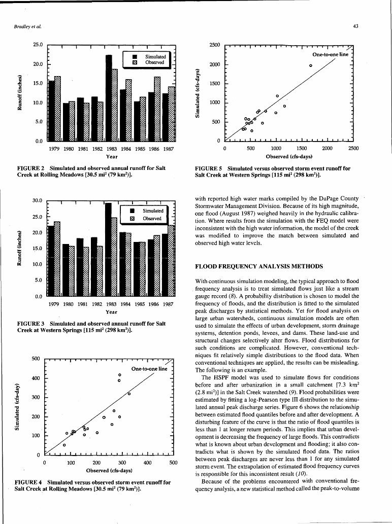
Bradley et al.

25.0

20.0

15.0

10.0

5.0

0.0

1979 1980 1981 1982 1983 1984 1985 1986 1987

Year

FIGURE 2 Simulated and observed annual runoff for Salt Creek at Rolling Meadows [30.5 mi2 (79 km2

)].

'ii .c: u

~ :t:: 0

~

30.0

25.0

20.0

15.0

10.0

5.0

0.0

1979 1980 1981 1982 1983 1984 1985 1986 1987

Year

FIGURE 3 Simulated and observed annual runoff for Salt Creek at Western Springs [115 mi2 (298 km2

)].

500

400

.>. "' "Cl "3 300 ..... ~ "Cl ~

"' 200 'S e ti}

100

0

0 100 200

0 0

300

One-to-one line

0

400

Observed (cfs-days)

500

FIGURE 4 Simulated versus observed storm event runoff for Salt Creek at Rolling Meadows [30.5 mi2 (79 km2)].

43

2500

One-to-one line

2000 0

j, "' "9 1500 {ll ..... ~ "Cl ~

1000 "' 'S

0

e ti}

500

0

0 500 1000 1500 2000 2500

Observed (cfs-days)

FIGURE 5 Simulated versus observed storm event runoff for Salt Creek at Western Springs [115 mi2 (298 km2

)].

with reported high water marks compiled by the DuPage County Stormwater Management Division. Because of its high magnitude, one flood (August 1987) weighed heavily in the hydraulic calibration. Where results from the simulation with the FEQ model were inconsistent with the high water information, the model of the creek was modified to improve the match between simulated and observed high water levels.

FLOOD FREQUENCY ANALYSIS METHODS

With continuous simulation modeling, the typical approach to flood frequency analysis is to treat simulated flows just like a stream gauge record (8). A probability distribution is chosen to model the frequency of floods, and the distribution is fitted to the simulated peak discharges by statistical methods. Yet for flood analysis on large urban watersheds, continuous simulation models are often used to simulate the effects of urban development, storm drainage systems, detention ponds, levees, and dams. These land-use and structural changes selectively alter flows. Flood distributions for such conditions are complicated. However, conventional techniques fit relatively simple distributions to the flood data. When conventional techniques are applied, the results can be misleading. The following is an example.

The HSPF model was used to simulate flows for conditions before and after urbanization in a small catchment [7.3 km2

(2.8 mi2)] in the Salt Creek watershed (9). Flood probabilities were estimated by fitting a log-Pearson type III distribution to the simulated annual peak discharge series. Figure 6 shows the relationship between estimated flood quantiles before and after development. A disturbing feature of the curve is that the ratio of flood quantiles is less than 1 at longer return periods. This implies that urban development is decreasing the frequency of large floods. This contradicts what is known about urban development and flooding; it also contradicts what is shown by the simulated flood data. The ratios between peak discharges are never less than 1 for any simulated storm event. The extrapolation of estimated flood frequency curves is responsible for this inconsistent result (10).

Because of the problems encountered with conventional frequency analysis, a new statistical method called the peak-to-volume

44

3 <I)

~ Q

Ii::

= • • Simulated Events

-0- Ratio of Flood Quantiles • ~ e c. 2 ~ ~ ~

~ • ~ ~ •• s 'a • .e ~ .... Q Q :a ~

0 2 5 10 25 50 100

Return Period (years)

FIGURE 6 Ratio of peak discharges before and after urban development. Circles show ratios for individual events; curve with boxes shows ratio of flood quantiles estimated using log-Pearson Type III distribution.

approach was developed for use with model-simulated flows (11). DuPage County uses a computer program, PVSTA TS, to do the peak-to-volume calculations. Another program automatically takes outputs from the FEQ model simulations of continuous simulation and extreme storm events and creates the input files needed byPVSTATS.

The idea behind the peak-to-volume approach is to estimate both the distribution of flood volume and the distribution of flood peaks conditioned on flood volume. At the site of interest, flood volumes are extracted from the continuous simulation for storms that produce a flood peak above a specified threshold u. A probability distribution Gu(x) is then fitted to the flood volumes. This step exploits the fact that flood volumes often conform to commonly assumed probability distributions, even when the flood peaks are affected by flow regulation and other complications. PVSTA TS allows users to choose between four theoretical probability distributions for Gu(x).

The next step is to estimate the distribution of flood peak Y conditioned on flood volume X. First, a statistical model is developed for the relationship between flood peaks and flood volumes. The relationship is assumed to have the form of a nonlinear regression model:

ln Y = W (ln X) + E (1)

The regression model errors E are assumed to be independent and normally distributed with mean zero and constant variance er~. The distribution of flood peak conditioned on flood volume is then a lognormal distribution truncated below the threshold u, or

Frix(ylx) = <1> [Z(y)] - <l>[Z(u)] x > 0 y > u 1 - <l>[Z(u)] ' - ' - (2)

where <1>( ) is the cumulative distribution function for a standard normal random variable, and

ln y - W(lnx) Z(y) = (3)


The critical innovation in this step is the use of information from extreme storms that have occurred in a meteorologically homogeneous region containing the watershed. These storms are used to simulate large floods, and the results are used to define the upper tail of the relationship between flood peak and volumes.

Finally, the probability distribution of flood peaks is found by combining the estimated distribution of flood volume with the estimated distribution of flood peak conditioned on flood volume. The distribution of flood peaks is given by

(4)

where A is the mean number of floods annually, and Hu(Yp) is the conditional distribution of flood peaks. A flood is defined as an event in which the flood peak exceeds a fixed threshold, u. Hu(yp) is defined as

(5)

where gu(x) is the flood volume density function corresponding to the distribution Gu(x).

Iri essence, the peak-to-volume approach combines appealing aspects of both continuous simulation and design storm approaches. Continuous simulation allows engineers to see the effects of landuse changes and flood mitigation measures for a variety of realistic storms. However, the peak-to-volume approach avoids problems in flood estimates that arise when conventional frequency analysis is applied. As with design storm approaches, large floods are simulated using extreme rainfall. However, the peak-to-volume approach uses actual storm events and incorporates the simulation results within a sound probabilistic framework.

Another clear advantage of the approach is that for floodplain mapping the statistical analysis can be carried out directly on peak flood stages (instead of peak discharges). This is especially important when there are backwater and floodplain storage effects that produce a nonunique relationship between peak stage and discharge. In a case study comparing the peak-to-volume approach with the design storm approach and conventional frequency analysis, the peak-to-volume approach produced the most credible estimates for floodplain mapping (12).

GINGER CREEK EXAMPLE

The Ginger Creek floodplain mapping study was the first application of the new DuPage County flood analysis techniques. Ginger Creek is a tributary to Salt Creek (Figure 1) and has a drainage area of 15.0 km2 (5.8 mi2

). The watershed contains low-density residential housing, two golf courses, a major Interstate highway, and some undeveloped wetlands. Two lakes on the main stem and several culvert and bridge crossings regulate flows during floods. To develop the FEQ model input for Ginger Creek, survey crews measured 77 cross sections and all significant hydraulic structures. Comparisons between simulated and observed water levels were made for a single flood (August 1987) to calibrate the model.

In practice, land-use conditions are easier to determine than land cover. As a result, DuPage County has developed regional conversions between land use and land cover. for hydro logic modeling. Table 1 shows the distribution of impervious land, grassland, and

Bradley et al.

TABLE 1 Land-Use to Land Cover Conversions

Land Cover Categories Land-Use Categories Impervious (%) Grassland(%) Forest(%)

Hydraulically-connected Residential:

1/4 acre lots 28 67 5 1/3 acre lots 20 75 1 /2 acre lots 15 80 5 1 acre or greater 10 85 5

Non-hydraulically-connected Residential:

1/4 acre lots 6 89 5 1/3 acre lots 4 91 5 1/2 acre lots 3 92 5 1 acre or greater 2 93 5

Multi-family residential 50 40 10

Commercial/Industrial 85 15 0

Major road corridors 50 50 0

Other roads 100 0 0

On-line surface water 100 0 0

Office/Research 80 15 5

Open space determined case-by-case

forestland for a variety of land-use categories. Local slopes are used to distinguish between the three grassland types. For Ginger Creek, areas were assigned to each land segment on the basis of future land-use conditions. Land segment unit area runoff is then multiplied by the land segment area to produce catchment runoff for future conditions.

From the 40-year simulation record, 58 significant runoff events were found. Simulated runoff for these 58 events was routed through the Ginger Creek stream network by using the FEQ model. For the statistical analysis the top 40 flood peaks were determined at each cross section. A log-Pearson Type III distribution was then fitted to the 3-day flow volumes for these events. Note that 3-day flow volume can be used as a surrogate for flood volume with this approach (11). Figure 7 shows the estimated volume distribution for an example cross section.

Extreme storms that occurred in Illinois or bordering states were used in the extreme storm simulations. Each storm was simulated three times by using the dry, average, and wet initial moisture conditions determined for the month when the extreme storm occurred. Peak stage and 3-day flow volume results for the extreme storm simulations were combined with a sample from the continuous simulation. A nonparametric regression technique called LOWESS (13) was used to find the relationship between peak stage and 3-day flow volume. Figure 8 shows the fitted curve at the example cross section. Finally, the peak-to-volume curve was numerically integrated with the estimated volume distribution to estimate the peak stage distribution. Figure 9 shows the estimated 100- and 500-year return period water surface profiles for the lower stem of Ginger Creek.

IDSTORY AND MOTIVATION FOR CONTINUOUS SIMULATION MODELING

Continuous simulation modeling has a long history in the Chicago metropolitan area. The first application of continuous simulation

~ QI

~ QI bO fU

c;; ~ QI ~

1000.0

100.0 .01 .1 5 10 2030 50 7080 90 95 99 99.999.99

Probability ( % )

FIGURE 7 Three-day flow volume distribution for Ginger Creek cross section. Log-Pearson Type III distribution was fitted to sample by method of moments.

11

10

9

8

7

6

5

45

100 1000

3-Day Flow Volume (cfs-days)

FIGURE 8 Peak stage and 3-day flow volume for Ginger Creek cross section. Circles show results from 40-year continuous simulation; crosses show results from simulations with extreme storms; solid curve shows regression made using LOWESS. Notice leveling off of peak stages for large floods due to floodplain effects.

650 L..J..J...l...L..L..1...J...l...L..L..1....L.J...L.L..L.L.1.-'-L..L..L..L-'-L...l.....L..L~

1000 2000 3000 4000 5000 6000 7000

Station (feet)

FIGURE 9 Estimated 100- and 500-year return period water levels for lower stem of Ginger Creek.

46

was in the late 1960s, with a study of the West Branch Chicago River. The 208 water quality studies of the late 1970s applied continuous simulation to many watersheds in northeastern Illinois (14). DuPage County's involvement with continuous simulation began in the 1980s with a study of Winfield Creek, a tributary to the East Branch of the DuPage River.

A study of Salt Creek in the late 1980s showed the utility of continuous simulation modeling for flood design in DuPage County. The study included analysis of the effects of modified outlet structures on Busse Woods, major flood control reservoir (2). Many were concerned that changing the outlet would increase the duration that sensitive woodlands in a bordering wilderness preserve would be inundated. Continuous simulation allowed engineers to estimate and compare flood inundation durations for many outlet designs.

Other major flood control projects now planned for Salt Creek also involve complicated hydraulic structures and operating schemes. A new flood control reservoir is being built; an abandoned quarry is being converted for flood storage along the main stem; a floodgate is being constructed to prevent Salt Creek backwater from flooding a tributary stream. The temporal and spatial patterns of rainfall, as well as the sequence of storm events, can significantly affect the operation of these flood control structures. Floodplain storage and backwater effects are also important on the low-gradient streams in the county. These complicated watershed conditions motivated DuPage County to choose a continuous simulation approach to provide the critical information needed for flood design (J). Recently adopted ordinances now require this approach for flood analysis and floodplain mapping on all major streams in the county.

CONCLUSION

DuPage County has turned to a continuous simulation modeling approach to handle the complicated flood analysis problems encountered in its large urban watersheds. The DuPage County method uses the HSPF model, a continuous simulation hydrologic model that has been calibrated to local conditions by using available stream gauge records. Land segments were created to represent the rainfall-runoff response for the five dominant land cover categories found in the county. Forty years of runoff have been generated for each land segment. Engineers simulate individual streams in the county using the FEQ model, an unsteady fl.ow routing model. Based on an analysis of land-use conditions for the stream, the FEQ model multiplies land segment runoff by the appropriate segment area and simulates flows and water levels for the stream. PVST ATS takes .FEQ model simulation results and estimates flood probabilities by the peak-to-volume approach.

In most counties across the United States, the design storm method is the standard approach for flood analysis. The design storm method is popular because it is easy to apply and has been widely accepted for flood analysis. Clearly, one of the greatest obstacles to implementing DuPage County's method has been the natural reluctance of some to accept new approaches. In the past continuous simulation approaches have been criticized for technical, financial, and administrative reasons (15). Yet the authors believe that many of the old criticisms of continuous simulation do not apply here.

By using DuPage County methods, the land-use data required to estimate land segment areas are the same as those required for other hydrologic methods. The cross-sectional input data required for the FEQ model are also the same as those required for steady-state


hydraulic models. Instead of running a single design storm event, engineers now run the FEQ model with data files containing the runoff for the continuous simulation and extreme storm events. Computer programs take simulation results and prepare inputs for the peak-to-volume flood frequency analysis. Unsteady fl.ow modeling does require more time and technical expertise. Still, the huge financial expenditures needed to mitigate the severe flooding problems in DuPage County warrant the additional time required to do a more detailed flood analysis.

ACKNOWLEDGMENTS

This work was supported by DuPage County, Illinois, Stormwater Management Division. Two of the authors (K. Potter and A. Bradley) were also supported in part by a grant from the National Science Foundation. This support is gratefully acknowledged. Many others have played key roles in this effort over the years. The authors are indebted to them for their contributions.

REFERENCES

1. Sikora, J. H., and J. H. Steffen. The Use of Continuous Simulation and Unsteady Flow Modelling in DuPage County, Illinois, In Urban Hydrology (M. E. Jennings, ed.), American Water Resources Association, 1991.

2. Busse Woods Reservoir-The Benefits and Costs of Additional Flood Control. Division of Water Resources, Illinois Department of Transportation, 1989.

3. Johanson, R. C., J.C. Imhoff, J. L. Kittle, Jr., and A. S. Donigian, Jr. Hydrological Simulation Program-FORTRAN (HSPF): Users Manual for Release 8.0. Report EPA-600/3-84-066. Environmental Protection Agency, 1984.

4. Hydrocomp Simulation Programming: Operations Manual. Hydrocomp, Palo Alto, Calif., 1976.

5. Crawford, N. H., and R. K. Linsley, Jr. Digital Simulation in Hydrology: Stanford Watershed Model IV. Technical Report 39. Department of Civil Engineering, Stanford University, Calif., 1966.

6. Franz, D. D. Unsteady Flow Solutions, Input Description for FEQ: Version 6.1. Linsley, Kraeger Associates, Ltd., Mountain View, Calif., 1990.

7. HEC-2 Water Surface Profiles, User's Manual. Hydrologic Engineering Center, U.S. Army Corps of Engineers, Davis, Calif., 1982.

8. Thomas, W. 0., Jr. Comparison of Flood-Frequency Estimates Based on Observed and Model Generated Peak Flows. Proc., International Symposium on Flood Frequency and Risk Analysis, Louisiana State University, Baton Rouge, 1986.

9. Dreher, D. W., G. C. Schaefer, and D. Hey. Evaluation of Stormwater Detention Effectiveness in Northeastern Illinois. Northeastern Illinois Planning Commission, Chicago, 1989.

10. Bradley, A. A., and K. W. Potter. Flood Frequency Analysis for Evaluating Watershed Conditions with Rainfall-Runoff Models. Water Resources Bulletin, Vol. 27, No. 1, 1991, pp. 83-91.

11. Bradley, A. A., and K. W. Potter. Flood Frequency Analysis of Simulated Flows. Water Resources Research, Vol. 28, No. 9, 1992, pp. 2375-2385.

12. Bradley, A. A., P. J. Cooper, K. W. Potter, and T. Price. Floodplain Mapping Using Continuous Hydrologic and Hydraulic Simulation Models. Water Resources Bulletin, submitted for publication.

13. Cleveland, W. S. Robust Locally Weighted Regression and Smoothing Scatterplots. Journal of the American Statistical Association, Vol. 74, 1979, pp. 829-836.

14. Areawide Water Quality Management Plan. Northeastern Illinois Planning Commission, Chicago, 1979.

15. Franz, D. D. Hydrologic Design: Extending Traditional Methods. In Hydraulic Engineering '93 (H. W. Shen, S. T. Su, and F. Wen, eds.), ASCE, 1993.



Small Urban Watershed Use of Hydrologic Procedures

VERNON K. HAGEN

The Federal Interagency Hydrology Subcommittee has published documents on flood frequency for gauged and ungauged watersheds. These documents include information on the preparation, dissemination, and results of a questionnaire sent to users of hydrologic methods. The questionnaire was circulated by a working group of the Hydrology Subcommittee and pertains to urban watersheds with areas of less than 30 mi2• Respondents provided information relative to the physical and administrative factors influencing their use of specific hydrologic methods. Although respondents did not cite all available hydrologic methods, most commonly used methods were mentioned, even though some were not actually used during the period of usage about which the respondents were questioned. Results of the questionnaire indicated that 86 percent of studies performed by hydrologic methods were performed by one of four methods. More than half of the studies conducted during -a 1-year period used the TR-55 computer model of the Soil Conservation Service (SCS). The other three methods in order of popularity were the rational method, TR-20 by SCS, and regression equations by the U.S. Geological Survey. The questionnaire displayed rather dramatically that users have been opting for less involved methods. The method selection process may be due to the fact that mutually accepted guidance on the priority of method use is unavailable. In addition to the results from the questionnaire, supplemental information is provided on the methods being used in state highway departments and the National Flood Insurance Program. Some current problems facing administrators regarding the proliferation of hydrologic models and rainfall data documents are also included.

Within the federal government lead responsibility for coordinating water data acquisition activities resides with the U.S. Geological Survey's (USGS's) Office of Water Data Coordination. The Interagency Advisory Committee on Water Data is composed of representatives of federal agencies and is divided into functional subcommittees (Figure 1). Among these subcommittees is the Federal Interagency Hydrology Subcommittee. Under the purview of the Hydrology Subcommittee is the coordination and the development of guidance for the application of hydro logic methods. Two important documents relating to hydrologic methods for flood frequency analysis were published in the 1980s by the Hydrology Subcommittee. The first document, Guidelines for Determining Flood Flow Frequency, Bulletin 17B, was published initially in March 1976 and most recently in March 1982 (1). These guidelines provided methods for obtaining the frequency of flood peak discharges for watersheds with gauged records of homogeneous data extending for 10 years or more. A follow-on publication, Estimating Peak Flow Frequencies for Natural Ungaged Watersheds-A Proposed Nationwide Test, was issued by the Hydrology Subcommittee in 1981 (2). The second document provided a classification of the procedures and results of a pilot test of several methods. It concluded that a massive nationwide test is needed to provide an authoritative basis

Dewberry & Davis, 8401 Arlington Boulevard, Fairfax, Va. 22031-4666.

for procedure selection and to recommend a national guide for ungauged watersheds.

The use of Bulletin 17B (1) has been extensive since its publication for gauged watersheds. However, its methods apply to special conditions that are not often found in urban watersheds. Homogeneous peak discharge data are generally not available for watersheds experiencing urban development. Urban flood information studies usually require complete hydrographs for stream and storage routings analyses. Therefore, the guidance in Bulletin 17B will generally not suffice in the small urban watershed situation. Although the ungauged watershed report provided information on some available hydrologic methods, it did not include information regarding the extent of use for various methods in present-day engineering practice. Many hydrologic studies are being performed on small urban watersheds for planning, design, land-use. regulations, flood insurance, and other purposes. A potpourri of methods are available, but limited guidance is offered on which methods are appropriate for various sets of conditions. Thus, it is difficult for administrators and managers to know when reasonable results are available. With the prevailing problems in mind, the Hydrology Subcommittee formed a working group to evaluate the prospects for providing guidance on small urban watersheds.

The purpose of this paper is to identify hydro logic methods commonly applied to analyses of flood flows in small urban watersheds. This paper is not intended to provide guidance or recommendations on the application or selection of hydrologic methods for various water resource purposes, including flood frequency analysis. Information is presented on the applications of hydrologic methods for small urban watersheds as developed from responses to a questionnaire distributed by the Hydrology Subcommittee. The questionnaire was to provide the first step in developing guidance on the appropriate use of the methods. It is unlikely that consensus guidance on the application of hydrologic methods for small urban watersheds will evolve in the near future; however, groups of experts continue to be formed to further this objective. Sound guidance is an elusive objective cloaked in controversy and thus requires time, effort, funding, and compromise.

SUMMARY OF QUESTIONNAIRE

From an evaluation of questionnaire responses, the author made some general observations concerning the estimation of hydrologic flood flows for small urban watersheds. Among the most revealing observations are that

• Practitioners may not be fully aware of some of the effective methods available for analyzing small urban watershed flood flows;

• Practitioners tend to use methods with which they have the greatest familiarity;


U.S. Department of Interior - Geological Survey >---

Yater Resources Division Office of Yater Data Coordination

Inter agency Advisory - Advisory Committee Committee on Yater Data for

on Public Use Yater Data (IACYD) (ACYDPU)

I Automated Hydrology Data Systems - ----- Subcommittee

I Working Groups

I Subcommittee

Yater-Data & - - Ground-Water Information Subcommittee

Exchange Subcommittee

Yater-Use - - Sedimentation Information Subcommittee

Suhcommittee

Working Coordinating Council for Yater-Groups Data Acquisition Methods

(IACYD Membership)

Small Technical Working Urban Groups for

Yater sheds Recommended Methods

FIGURE 1 Organizational chart.

• Procedures for rural watersheds may be in use without adjusting for the impacts of urbanization;

• Some practitioners are apparently not using the most recent version of the hydrologic models; and

• There appears to be a tendency to use less involved methods.

Although these observations are deducted from responses provided on the questionnaire and would require further communication with the respondents to verify and explain the observations, they do point to the need for the development of generally accepted guidelines for hydrologic method applications. For example, the application of procedures developed for rural areas to an urbanized watershed can result in significant underestimation of flood flows. Use of something other than the most recent version of a hydrologic model may not seriously affect the results, but it may be an inefficient means of study. Practitioners must also use care in the selection of methods. Less involved procedures may be satisfactory for most situations; however, the consequences of cursory estimates are important considerations in the level of effort devoted to the computation of synthetic floods.

A possible implication of the results of the questionnaire is that the conclusions of the report on ungauged watersheds (2) may be influencing decisions about the selection of hydrologic methods. Since funding of the nationwide test was not provided and does not appear likely, the hydrologic community must deal with the conception that a nationwide test is the only mechanism for an authoritative national guide on hydrologic methods for ungauged water-

sheds. Study managers apparently have a difficult task in convincing decision makers that an in-depth hydrologic method should be used in the face of the previous conclusion that results cannot be scientifically proven to be better than those obtained by a less demanding method. Although scientific proof of the superiority of some methods over others, given a specific set of conditions, may not be readily obtainable, technical expertise and experience can be used to provide guidance on which methods are more likely to give consistently good results. Therefore, guidance on the selection and application of hydrologic methods for flood estimates of small urban watersheds appears to be needed as soon as practicable.

PROFESSIONAL SOCIETIES

Expertise in the application of hydrologic methods is available within the public, private, and academic sectors. Professional society membership normally reflects a cross section of these sectors. Journal articles, committee reports, and proceedings of professional meetings offer extensive literature related to hydrologic methods. Many of these documents, as well as publications of the federal government, are available through the National Technical Information Service, U.S. Department of Commerce, 5285 Port Royal Road, Springfield, Virginia 22161.

On the basis of questionnaire responses, which indicate a need for more information on microcomputer hydrologic models, and needs for storm water management practices, the work of two professional societies is described briefly in the following sections.

Hagen

American Society of Civil Engineers

The membership of ASCE contains many engineers who are engaged in hydrologic studies. They include practicing private firms, educators, and researchers as well as local, state, and federal agencies. Being concerned about professional integrity and sound engineering practices, ASCE has directed significant effort in the field of urban water resources. Toward this effort ASCE has established several committees that deal with the hydrology of small urban watersheds.

The ASCE Task Committee on Microcomputer Software has sent questionnaires to vendors regarding available models for urban hydrology analyses and details about their application. Results of the survey were presented at the National Conference on Hydraulic Engineering in New Orleans, Louisiana, August 14-18, 1989.

American Geophysical Union

The American Geophysical Union (AGU) may be described more as a scientific organization than a professional society, because its members and activities are generally oriented toward research. However, its Hydrology Committee is one of the strong elements of the organization and is deeply involved in urban hydrology. This committee published a monograph (3) on state-of-the-art practices in the field of urban hydrology and storm water management. Another example of AGU Hydrology Committee efforts in urban watersheds is sponsorship of personal computer workshops on methods for flood frequency analysis and flood forecasting. This activity was provided during the International Association of Hydrological Sciences, Third Scientific Assembly, May 10-19, 1989, Baltimore, Maryland.

USER'S NEEDS

Present Use of Urban Flood Frequencies

Urbanization of watersheds increases the percentage of impervious land area, with the direct result of increased volumes of runoff from rainfall events. The increased volume of runoff may be accompanied by higher flood peaks and increased, possibly erosive, flow velocities. The consequences of this cause-and-effect relationship between urbanization and increased runoff have required organizations involved in the planning, management, and maintenance of urban areas to become knowledgeable of hydrologic analysis.

Transportation planners and design engineers have a keen interest in flood volume and frequency with regard to water conveyance through bridge openings and culverts. Protecting costly bridge structures and embankments from damage due to overtopping is a critical design item. Planning for watershed changes over the proposed life of structures is difficult, but it is an important task. For example, a culvert in a rural area designed to pass a 100-year flood flow may be adequate to pass only a 50-year flood after urban development of the watershed.

In response to increasing losses from flooding throughout the nation, the U.S. Congress established the National Flood Insurance Program (NFIP) through the National Flood Insurance Act of 1968. Under the mandate of NFIP, administered by the Federal Emergency Management Agency's (FEMA' s) Federal Insurance Administration, studies of 100-year flood hazards have been conducted for

49

all flood-prone communities. The results of those studies provide the basis for management of flood risk areas and the provision of flood insurance to homeowners and non-residential building owners within communities that participate in NFIP. The issuing of building permits, community zoning issues, and land development are among the activities affected by flood frequency analyses conducted as part of a flood insurance study for NFlP.

Economic justification, design, and operations of flood control projects require flood information. Storm drainage facilities are usually designed with floods of a specific frequency in mind. These activities and others require information on floods in order to proceed in an orderly fashion. Incorrect analysis of floods can involve excessive expenditures or could result in serious damage to facilities based on underestimated flood magnitudes and frequencies.

Planning Future Hydrologic Studies

The nature and direction of future urban hydrologic studies should be shaped through insights gained from an examination of the amount of use given to various flood analyses for urban watersheds. Serious questions may evolve from this examination, such as the following:

• Are users taking advantage of the state-of-the-art practice? If not, what are the reasons for limited use of apparently more effective methods?

• Is the state of the art adequate for user needs? If not, what direction should research and development take?

• Does user response to the questionnaire reflect real-world applications of various hydrologic models? If not, what would

' cause the results to be skewed? • Do the questionnaire results indicate the need for coordinated

guidance on the use of hydrologic models? If so, who should provide this guidance and what should be the extent of the guidance?

Although this paper is not of the scope needed to answer these and other pertinent questions, activities of other organizations may help to resolve some of the questions. For example, the Water Science and Technology Board of the National Research Council sponsored a committee report entitled Opportunities in the Hydrologic Sciences ( 4). That committee report addressed items such as scientific development to the present, outstanding historical achievements, intellectual frontiers and scientific challenges, new data requirements, qualifications of the people needed, and an indication of applications.

ORGANIZATION OF WORK GROUP

Early Concepts

The Hydrology Subcommittee recognized the need for a working group on methods for analyzing flood flows from small urban watersheds. Agency interest was solicited by the subcommittee chairman, and an initial work group was established in 1982. This group included FEMA, the U.S. Army Corps of Engineers (USACE), Soil Conservation Service (SCS), USGS, Agricultural Research Service, Tennessee Valley Authority, and FHW A. The early activities of this group were devoted to the development of a statement of work. The objective of this activity was to develop

50

guidance on the selection of methods for analyzing flood flows from small urban watersheds. This objective was to be accomplished by a contractor who would review methods, consult with agencies and other users, and prepare a user's manual. The investigation was designed to include

• Watersheds (up to 30 mi2),

• Development (natural to 100 percent urban), and • Flow (peaks, volumes, hydrographs).

The final product was expected to identify methods of analyses and provide guidance on the selection and application of methods. Since the contractual arrangement was anticipated to involve considerable funding, the separate agencies investigated sources of funds that could be used to support this activity. Federal budgets are planned well in advance of receipt of an actual appropriation from Congress. Thus, a time-consuming process is involved, and competition for research-type funding is intense.

Questionnaire Status

In 1985 .the work group concluded that insufficient funds would be committed by the federal agencies to pursue a contracted study. Lacking full funding for planned activities, the work group agreed to pursue its statement of work on a limited basis with member support. Examining efforts that could be implemented by the task committee, information on the current use of methods became a high-priority item. Thus, the task committee began to prepare an appropriate questionnaire that could be circulated among the practitioners of urban hydrology. It was agreed that the questionnaire should glean enough information from users to help prepare future guidance on flood methods for urban watersheds. In February 1987 the parent Hydrology Subcommittee approved the task committee's recommendation to distribute the questionnaire to organizations experienced in hydrologic modeling. A distribution list was prepared; it included the following:

• Federal agencies on the Hydrology Subcommittee, • State agencies involved in water resources, and • Private contractors performing hydrologic analyses.

The distribution list did not include educational and research institutions because the information gathering was directed toward practitioner use rather than research and development. However, future efforts in guidance on the selection and application of hydrologic models would need to involve this segment of hydrologic experts. The questionnaire was mailed in February 1987. Although most responses were received in a timely manner, there were a few delays in the receipt of completed questionnaires.

RESULTS OF QUESTIONNAIRES

Respondent Information

Respondents to the questionnaire were grouped by their employers and are listed as federal, state, or private practitioners in hydrologic analyses. Figure 2 depicts the percentage distribution by the source of responses. It does not indicate the numbers of respondents, because many respondents provided information on more than one hydrologic method.


State (51.7%)

Federal (29.6%)

FIGURE 2 Source of responses.

Classification of Methods

Many hydrologic methods were identified in the responses to the questionnaire; however, the list does not include all available methods. To consolidate the responses for data management purposes, all responses were sorted to a classification system containing 12 categories. The individual hydrologic method was used as a classification title when significant usage of that method was indicated by answers to the questionnaire. Information on the classification of methods is provided in Table 1 and Figure 3.

Details on the numbers of studies performed in the year preceding completion of the questionnaire (1986) are given in Table 1. This is a 1-year sample and reflects neither variations in method use from one year to another nor a longer-term summary of method use.

Reasons for Selection of Method

Table 2 provides an interesting comparison among methods regarding the most prevalent reasons given for using a particular hydrologic method. Review of such information is important in planning a strategy for obtaining guidance on the selection of hydrologic methods. Obviously, an individual user will not benefit from selection guidance if an agency or customer dictates the method that is to be used for a specific study. The user and client may, however, benefit from application guidance. Although the results of this activity provide good general information, technical information such as reliability and reproducibility of results is probably best obtained via an expert systems approach.

Response Regarding Physical Features

The United States has a wide variety of physical features that influence the amount and rate of runoff from a watershed. Several of these features were included in the questionnaire, and responses reflect the peculiarities of different parts of the country. Physical feature~ included in the questionnaire were watershed size, slope of terrain, type of soil cover, density of vegetation, and annual precipitation. Responses on this aspect are not included in this paper; however, a careful review of this information by experts in hydrologic analysis could provide insight on the proper use of a hydrologic method for the environment in which it was used. Such information is important to the criticality of completing guidance on the selection and application ofhydrologic methods. When physical features

Hagen 51

TABLE 1 Classification of Methods

TR-55 10,763 51.3

2 Rational 4,054 19.5

3 TR-20 1,954 9.3

4 USGS Rural Regression F.quations 1,265 6.0

5 USGS Urban Regression F.quations 529 2.5

6 FHW A Small Rural Watersheds

7 HEC-1

8 Log-Pearson Type ill

9 SCS Hand Methods

10 . Synthetic Flood Frequency

11 Other Runoff Hydrograph Models

12 Miscellaneous

TOTAL

and the use of hydrologic models are considered, other aspects not addressed by the questionnaire should also be considered. Some of these important aspects are watershed shape (long and narrow basins have longer response times than short and wide basins); many methods do not have the capability to combine and channel route subbasin runoff; others do not provide the ability to route runoff through storage.

CONCLUSIONS FROM RESPONSES

After examining the responses to the questionnaire, the author drew some general conclusions regarding the use of hydrologk methods as applied to small urban watersheds. Other analysts experienced in hydrologic models may arrive at different conclusions. Some of the more obvious conclusions are as follows:

.• The number of studies performed in a I-year period (20,000 plus) indicates that there is a great deal of activity in hydrologic analyses of small urban watershed.

• Calibrated rainfall runoff models such as TR-20 and HEC-1 constitute a small percentage (12 percent) of all models used.

w

"' :::> ~. z w (.) a: w a..

60

50

40

30

20

10

0 2 3 4 5 6 7 8 9 10 11 12

CLASSIFICATION

FIGURE 3 Use of hydrologic methods.

500 2.4

485 2.3

360 1.7

219 1.0

155 0.7

138 0.7

553 2.6

20,975 100.0

TABLE 2 Reasons for Selection of Method

RESPONSE RANKING

CLASSIFIED METHOD

TR-SS

Rational

TR-20

USGS Rural Regression Equation

USGS Urban Regression Equation

FHW A Small Rural Watersheds

HEC·l

Log-Pearson Type ill

SCS Hand Methods

Synthetic Flood Frequency

Other Runoff Hydrograph Models

Miscellaneous

Legend:

A - Economic Feasibility B - Required by Regulations C - Specified in Contract

1 2 3

F E A

F E A

E F D

F E A

F E A

F

E F A

F E A

F E A

F E A

E F D

F E A

D - Unique Environment E - Organi7.ational Familiarity F - Ease of Use

4

D

B

A

D

D

D

B

D

D

A

D

s 6

B c D c B c B c B c

B c P .. c

--

B c B c

• Practitioners of hydrologic analysis are interested in the procedures being used by their peers, because 94 percent of the respondents requested copies of the result(s) of the survey.

• Ease of use was the most prominent response regarding the reason for selection of methods.

• Respondents generally do not view small urban watersheds as unique environments because this reason for method use ranked midway in responses.

• Results of the survey confirm the need for guidance on the selection and application of hydro logic methods for flood frequency analysis being applied to small urban watersheds.

OTHER ASSESSMENTS OF HYDROLOGIC METHODS

Since the Federal Interagency Hydrology Subcommittee survey of hydrologic methods was summarized in 1989 and has not been

52

published for general information, it appeared prudent to supplement the results of that survey with additional and more recent information. Data from two individual assessments are provided for comparison.

State Highway Departments

Probably thousands of hydrologic computations for sizing highway water passages (culverts and bridges) are made each year. Sizes are generally based on specific quantiles (peak flows and their associated exceedence frequencies). This survey conducted by the Maryland State Highway Administration in 1990 included 45 states and the hydrologic methods used by their highway departments. Table 3 gives the hydrologic methods cited and the number and percentage of states that use them.

Some interesting observations from this survey are that

• Eighteen states indicated the use of only one hydrologic method in their engineering analyses of waterway openings;

• Three states use five different hydrologic methods; and • Thirty-three states use hydrologic methods that produce only

peak flows (hydrographs are not available from the methods selected).

This survey did not include information on the reasons that specific hydrologic methods were selected. However, from examination of the methods selected, it appears that simplicity of use, consistency of results, and nonuse of hydrographs are important considerations. Because of the limitations of this survey, it appears that state highway departments do not become involved in detailed hydrologic analyses. This assumption may be correct for most of the states surveyed; however, it is certainly not true for the Illinois Department of Transportation (IDOT). IDOT is an example of a state highway organization that has a leading role and responsibility for sound hydrologic analyses within the state. For those states that do not have a lead agency for coordinating and ·reviewing hydrologic analyses, IDOT serves as an example of how state highway organizations can provide this important service. Although several federal agencies and other state agencies may be performing hydrologic studies within a state, there may be no state agency with responsibility or adequate funding to coordinate studies and to maintain some level of consistency throughout the state.

National Flood Insurance Program

Most of the communities in the NFIP have base (100-year) floods included in their flood insurance studies (FISs). Thus, FEMA is currently more in a revision mode than in its earlier development mode insofar as hydrologic studies are involved. The majority of revision studies involving hydrologic analyses are performed by engineering firms that represent owners of property within the designated 100-year floodplain. These property owners are seeking relief from NFIP by convincing FEMA that their estimate of the 100-year flood is more correct than the estimate in the FIS. Dewberry & Davis (D&D) serves as a technical evaluation contractor for FEMA Regions 1 through 5. In this role D&D reviews the technical adequacy of hydrologic studies in revision requests as well as those studies performed by FEMA's study contractors who update FISs. A survey of the hydrologic methods being used in review cases was


TABLE 3 Use of Hydrologic Methods by State Highway Departments .

Regional Regression Equations 36 80 (USGS)

Rational (Mulvaney's Equation) 19 42

Bulletin 17-B (Interagency 18 Hydrology Subcommittee)

other Methods (Used by One 7 16 State)

TR-55 (SCS) 6 13

TR-20 (SCS) 4 9

HEC-1 (USACE) 7

FHWA Procedures 7

conducted during August 1993 for Regions 1 through 5. Results of that survey are included in Table 4.

An earlier survey of the hydrologic methods used during FEMA's development mode would have resulted in a table more consistent with that showing the results of the state highway department survey. Less use of rainfall runoff models such as HEC-1 and TR-20 would have been reported. Although the FEMA survey shows HEC-1 as the most prominent hydrologic model used, in many instances the HEC-1 model uses the curve number loss function and unit hydrograph procedure from TR-20. HEC-1 does not include the Att-Kin routing procedure from TR-20 as one of its routing options. Therefore, it is difficult to obtain exactly the same results from the two models unless hydrograph routing is not involved.

Another observation not available from the survey is that the Kinematic wave option available in HEC-1 is seldom used in hydrologic studies submitted to FEMA in the eastern half of the United States. The reasons for the lack of popularity of this valuable urban hydrology procedure are not readily apparent. However, unfamiliarity with the procedure and more intense input requirements could be deterrents.

RAINFALL DATA AND AVAILABLE MODELS

Those who are part of water resource programs being administered by various federal, state, and local organizations face important decisions regarding the use of hydrologic models and rainfall data. The traditional rainfall probability relationships published by the National Weather Service (NWS) many years ago are being updated

TABLE 4 Hydrologic Methods Used by FEMA, Regions 1to5

'''~.EijgpiQJ.A91g!~q?st?;,:' l'ffl!MB~'.:()ij;~U?.St HEC-1 (USACE) 34 25

Regional Regression Equations 28 . 21 (USGS)

Bulletin 17B (Interagency 25 18 Hydrology Subcommittee)

TR-20 (SCS) 23 17

Rational (Mulvaney's Equation) 10 7

TR-55 (SCS) 6

Others (used in one study) 6

TOTAL 136 100

Hagen

in parts of the United States. However, funds are not available for a complete revision of these important documents. In fact, several years of study and revision would be needed to complete such an undertaking if all needed funding was available, thus the need for decisions on the use of new data developed by a group other than NWS. The state of Illinois has directed that its Bulletin 70 be used when performing hydrologic studies within the state. Other entities have performed rainfall probability studies for use in lieu of the NWS documents. Although special rainfall studies may provide more up-to-date information, they can create problems for federal or state programs insofar as consistent results are concerned. This is especially true when in-depth detailed analyses are not involved.

Development of new hydrologic models also causes concern for administrators and technical experts attempting to become proficient in the use of the large array of models available. When the new models are developed within federal agencies that support the models by correcting errors and adding improvements, concerns are less dramatic. However, when model development is by private individuals or through research grants, there is much less opportunity for continuing support and improvement. FEMA has established rules for the use of hydrologic models in NFIP; however, many of those requesting revisions submit proposed changes that are based on the use of models that do not comply with FEMA rules. This can cause property owners considerable expense in redoing the studies or going through the process of obtaining FEMA' s approval for the use of the model. Many federal agencies, such as the USGS, USACE, SCS, and FHW A, have their own hydrologic models that were designed for the specific needs of the agencies. However, many of these models are used by the private sector, often with some add-on modules that increase the total number of models·

53

available for use. Thus, organizations without their own hydrologic models are confronted with the difficult task of selecting or approving models for use in their programs. Presentations on specific hydrologic models, suc.h as these being made for TRB, are useful for those individuals evaluating models for use or approval. Although these presentations are only a sample of the available hydrologic models, sorting out the pros and cons of the different models is a formidable task. Two of the presentations involve models used extensively as indicated by the surveys that were conducted; however, the other two models are more involved, and their use is probably limited to individuals highly trained in their application. Interest in SCS and USACE models will be related more to their practical applications, whereas interest in the other two models (DR3M and HSPF) will tend toward scientific applications.

REFERENCES

1. Guidelines for Determining Flood Flow Frequency, Bulletin 17B. Hydrology Subcommittee, Interagency Advisory Committee on Water Data, Reston, Va., March 1982.

2. Estimating Peak Flow Frequencies for Natural Ungaged WatershedsA Proposed Nationwide Test. Hydrology Committee, U.S. Water Resources Council, Washington, D.C., 1981.

3. Water Resources Monograph Urban Stormwater Hydrology (D. F. Kibler, ed.), Hydrology Committee, American Geophysical Union, Washington, D.C., 1982.

4. Opportunities in the Hydrologic Sciences (P. S. Eagleson, ed.), Water Science and Technology Board, National Research Council, Washington, D.C., 1991.



Urban Hydrology Design Using Soil Conservation Service TR-55 and TR-20 Models

NORMAN MILLER AND DONALD WOODWARD

The Soil Conservation Service for many years has been using two computer models for urban hydrology planning and design: Computer Program for Project Formulation-Hydrology (TR-20) and Urban Hydrology for Small Watersheds (TR-55). The needed revisions to TR-20 do not directly affect its application in urban areas, whereas the proposed revisions to TR-55 could affect the peak discharges. The primary change is in the velocity method for computing time of concentration, which deals with the sheet flow and concentrated flow.

The Soil Conservation Service (SCS) has two watershed computer models that can be used in urban hydrology design: Computer Program for Project Formulation-Hydrology (TR-20) (1) and Urban Hydrology for Small Watersheds (TR-55) (2). The TR-20 computer program was developed in 1965 and has been modified several times since then. The TR-55 document was initially issued in May 1975 (3) and was revised and issued with a computer program in June 1986 (2); it has not been modified since then.

GENERAL

TR-20 (1) is a more complex computer model that

• Develops hydrographs, • Routes hydrographs through reservoirs, • Routes hydrographs through valley reaches, and • Adds hydrographs.

TR-55 is a simplified procedure that uses the results from running TR-20. The calculations can be performed without using a computer. TR-55 does not develop or route individual hydrographs.

Neither model is to be used for storm sewer design, but the models can be used to show the effects of urbanization on the peak rates and volumes of runoff. In urban situations they are used most often to design or plan storm water management structures.

INPUT

TR-20 and TR-55 both require the same basic inputs of runoff curve number (CN), time of concentration (Tc), and drainage area (DA) for computation of peak discharge and the volume of runoff for a specific rainfall distribution. TR-20 allows the user to define the rainfall temporal distribution. TR-55 has four design rainfall dis-

N. Miller, Engineering Division, Soil Conservation Service, P.O. Box 2890, Washington, D.C. 20013. D. Woodward, Ecological Sciences Division, Soil Conservation Service, P.O. Box 2890, Washington, D.C. 20013.

tributions. In dealing with smaller drainage areas, the principal concern among the three variables CN, T.:, and DA is T.:.

Time of Concentration

The original TR-55 (3), published in 1975, had two methods for calculating T.:: the lag method and the velocity method. The velocity method involved computing the travel time for overland flow, storm sewer or road gutter flow, and channel flow. The 1986 version (2) changed the procedure for computing overland flow and eliminated storm sewer or road gutter flow. Both methods of estimating T.: are described in the following sections.

Lag Equation

The lag equation is strictly empirical and was developed from data from small agricultural watersheds. The flow from or in small agricultural watersheds was' primarily overland flow, in comparison with primarily channel flow in large watersheds.

The lag equation is

(1)

where

Lag = lag (hr); Y = average slope of watershed-(%); S = [(1,000/CN') - 10], where CN' is the curve number; and L = hydraulic length of watershed (ft).

Velocity Method

The velocity method incorporates three kinds of flow: sheet, shallow concentrated, and channel. The sheet flow portion is of primary concern.

The time of travel (T,) for sheet flow is given as

where

T, = travel times (hr); n =Manning's roughness coefficient; L = flow length (ft);

P 2 = 2-year, 24-hr rainfall (in.); and S = slope of hydraulic grade line (land slope) (ft/ft).

(2)

Miller and Woodward

Equation 2 was developed from the Manning's kinematic solution using the four SCS standard rainfall distributions. The original kinematic wave equation included rainfall intensity as a variable. Several studies were done to develop a relationship between the standard design rainfall distribution, 24-hr rainfall amount, and maximum hourly intensity.

For shallow concentrated flow, a graph of average velocity versus watercourse slope for only paved and unpaved conditions is used. The velocity is translated into travel time. Velocity for s~allow concentrated flow assuming normal flow is given by the following generalized relationships:

V= 16.1345 (S)0·5 (3)

v = 20.3282 (S)0·5 (4)

These relationships assume that n is equal to 0.05 and the hydraulic radius is 0.4 ft for unpaved conditions and that n is equal to 0.025 and the hydraulic radius is 0.2 ft for paved conditions. They were developed assuming Manning's equation for wide rectangular channel conditions.

TR-55

The primary use for TR-55 is for before and after urbanization calculations. Therefore, the same 1'c method should be used for both before and after. It would not be rational or consistent to use the lag equation for before conditions (agriculture) and the velocity method for after conditions (urbanized). In addition, the velocity method is more accurate and physically based.

Thus, when TR-55 was revised in June 1986, the lag equation was eliminated and the velocity method was expanded, especially with the addition of sheet flow in the headwaters. Concern is principally with the guidance given to use Equation 2 for a sheet flow of less than 300 ft, which was meant to be a maximum. Many users employ 300 ft regardless of the nature of the ground surface and the condition of the surface. In most cases the maximum length should be much less than 300 ft, possibly in the range of 75 to 125 ft, depending on the surface conditions. For small watersheds this choice of sheet flow length can affect 1'c and the resulting peak discharge considerably.

TR-55 uses a short-cut routing procedure developed from routing of many storms through actual structures. The resulting regression equations were developed by a polynomial curve-fitting technique. The curves in Figure 6-1 in TR-55 are a function of both storm duration (24 hr) and rainfall distribution (Types 1, 2, 3, and la).

55

TR-20

The primary use ofTR-20 is for watershed planning and evaluation studies. These studies involve determining the economic evaluation of various alternative structure measures. Such structures could include improvements to flood-retarding structure channels and land treatment and use changes. TR-20 can also be used to simulate recorded hydrographs. It is assumed that the same 1'c calculation procedures will be used for all alternatives.

The velocity method for computing 1'c is used with TR-20. This is the procedure explained in detail in TR-55 and discussed earlier.

TR-20 uses the storage indication method of reservoir routing and is not limited by storm duration and rainfall distribution. The ATT-KIN procedure is used for channel routing. The ATT-KIN procedure uses actual reach length and actual cross-section rating curves.

TR-55 uses the ATT-KIN routing procedure with an assumed velocity for a selected reach length to give a fixed routing interval as shown in Exhibits 5-I, 5-IA, 5-II, and 5-III in TR-55.

FUTURE WORK

Proposed changes in the next revision of TR-55 are as follows:

• For sheet flow: -Give more guidance on the maximum length criteria, and -Give more surface descriptions and corresponding n-values.

• For shallow concentrated flow, add more curves for other surface conditions instead of grouping them all into unpaved-type conditions.

• A new version of TR-20 is being developed. The new version will correct minor program problems, update the user's manual, provide a new input program, and provide the documentation for the A TT-KIN channel routing procedure.

REFERENCES

1. Computer Program for Project Formulation-Hydrology. Technical Release 20. Soil Conservation Service, U.S. Department of Agriculture, 1982.

2. Urban Hydrology for Small Watersheds. Technical Release 55. Soil Conservation Service, U.S. Department of Agriculture, June 1986.

3. Urban Hydrology for Small Watersheds. Technical Release 55. Soil Conservation Service, U.S. Department of Agriculture, May 1975.



Hydrologic Engineering Center Models for Urban Hydrologic Analysis

ARLEN 0. FELDMAN

· The Hydrologic Engineering Center (HEC) has several numerical models for simulation of hydrologic and hydraulic processes in urban areas. New development and application procedures for the surface water hydrology models are described. The primary surface water hydrology model is the HEC-1 Flood Hydrograph Package. It can simulate the precipitation-runoff process in a wide variety of basins, from small urban areas to large river basins. It also has many features that facilitate its application to urban areas. The next generation of HEC-1, termed the NexGen Hydrologic Modeling System, is under development. A new model to analyze flooding in interior areas (e.g., on the land side of a levee) was just released. An older model (STORM) for urban storm water and combined sewer storage and treatment is still used in the profession, but it is not actively supported by HEC. These models (primarily HEC-1) are discussed in relation to urban hydrologic design. Future directions of the U.S. Army Corps of Engineers' new Urban Hydrology Methods/Models research work unit are also discussed.

As the U.S. Army Corps of Engineers' national center for hydrologic engineering and analytical planning methods, the Hydrologic Engineering Center (HBC) addresses the needs of Corps field offices. HBC has developed and supported a full range of simulation models for understanding how water resource systems function (J). It is assumed that experienced professionals c·an ·deduce the appropriate solution to a problem given the insight provided by selective execution of the simulation models. This deduction process has historically been and will continue to be the dominant methodology for planning and for making operational decisions in the water resources community.

This paper primarily addresses the urban hydrology software of HBC. Not included is information about HBC's river hydraulics, flood damage, flood frequency, reservoir system, and water quality models. In recent years many improvements have been made to the steady-state water surface profile model, the sediment scour and deposition model, and the unsteady flow model. In the area of flood damage analysis, a flood damage analysis package provides a comprehensive set of tools that can be used to evaluate flood damage reduction, and a new program accounts for project benefits during flood event operations. HBC also maintains a set of non-point source, river, and reservoir water quality simulation models.

The U.S. Army Corps of Engineers' flood control responsibility has applied to many geographic settings. The flood damages to be prevented are primarily in urban areas. HBC developed several computer programs and methods for analyzing and computing urban flood damage. The principal program is the Flood Damage Analysis Package (2). The subject of this paper is not the damage computation but the hydrologic simulation software (e.g., HEC-1) developed for urban areas. The Corps has made flood damage reduction investigations of just about every type of urban area, from sparsely

Hydrologic Engineering Center, U.S. Army Corps of Engineers, 609 Second Street, Davis: Calif. 95616.

developed areas to major metropolitan areas. For these studies traditional hydrologic models have been applied to the urban areas; often, new runoff parameters were added to the models to simulate the particular watershed characteristics of urban areas. Many of the computer simulation models are simply adapted to the particular infiltration, runoff, and channel characteristics of urban areas.

In the Corps Urban Studies Program of the 1970s, new models were developed to meet the specific needs of those studies. In other studies, for example, the Expanded Floodplain Information Studies, major changes in the use of geographic data were made; this was the start of geographic information system (GIS) usage in hydrologic modeling. In all cases HBC strives to develop physically based simulation models that are easily applied in ungauged areas. This is especially true in the urban situation. The following sections of this paper discuss the urban hydrology software development and application activities of HBC.

HEC-1 FLOOD HYDROGRAPH PACKAGE

Background

The HEC-1 Flood Hydrograph Package (3) computer program was originally developed in 1967 by Leo R. Beard· and other members of the HBC staff. The first version of the HBC-1 program package was published in October 1968. It was expanded and revised and was published again in 1969 and 1970. To simplify input requirements and to make the program output more meaningful and readable, the 1970 version underwent a major revision in 1973. In the mid-1970s, increasing emphasis was being placed on urban storm water runoff. A special version of HEC-1 was developed; this version incorporated the kinematic wave runoff techniques that were being used in several urban runoff models. Special versions of HEC-1 were also developed for other purposes. In 1981 the computational capabilities of the dam break, project optimization, and kinematic wave special versions were combined into a single package. In late 1984 a microcomputer [personal computer (PC)] version was developed. A menu capability was added to facilitate user interaction with the model; an interactive input developer, a data editor, and output display features were also added.

Current Version

The latest version, Version 4.0 (September 1990), represents improvements and expansions to the hydrologic simulation capabilities together with interfaces to the HBC Data Storage System (HEC-DSS) (see a later section of this paper). The DSS connection allows HEC-1 to interact with the inputs and outputs of many HBC and other models. (DSS will be an important capability for marry-

Feldman

ing several models needed for complex urban runoff situations, as discussed later.) New hydrologic capabilities in HEC-1 include Green and Ampt infiltration, Muskingum-Cunge flood routing, prespecified reservoir releases, and improved numerical solutions of kinematic wave equations. The Muskingum-Cunge routing may also be used for the collector and main channels in a kinematic wave land surface runoff calculation. This new version also automatically performs numerical analysis stability checks for the kinematic wave and Muskingum-Cunge routings. The numerical stability check was added because many users did not check the validity of the time and distance steps used in the model.

In September 1991 an alternative version of HEC-1 (Version 4.0. lE) was released for use on PCs with extended memories. A hydrograph array size of 2,000 time intervals is now available in this version. The increased array ~ize reduces the limitations encountered when simulating long storms using short time intervals. For example, simulation of a long (96-hr) storm in an urban area at 15-min intervals requires 384 ordinates just for the storm; more

time intervals would be required to simulate the full runoff hydrograph and to route it through the channel system. The large-array version also allows greater flexibility in checking for the numerical stability of simulation processes (e.g., kinematic runoff and routing computations). The large-array version uses an extended or virtual memory operating system available on 386 and 486 machines.

Urban Hydrology Features

Watershed Runoff

HEC-1 computes runoff using one of several loss methods (e.g., SCS curve number or Green and Ampt) together with either unit

z I

COLLECTOR CHANNEL

FIGURE 1 Elements used in urban-runoff calculations.

57

hydrograph or a kinematic wave. A Kinematic wave was added specifically to address the issues of urban hydrology. It also provided a better physical b~sis for application in ungauged areas. Before adding the kinematic wave runoff capability to HEC-1, the overall structure of urban runoff computations was analyzed. Urbanization impacts on both infiltration and runoff characteristics were considered. Also, the procedure for applying the model to large urban areas was reviewed. It was noted that runoff is usually computed· from two types of surfaces: pervious and impervious. Within a subbasin (the smallest land surface area for which precipitation-runoff calculations will be made), urban drainage systems were found to have a regular structure of overland flow leading to collector channels of increasing size. For example, runoff from. a property goes into a gutter and then into storm drains of various sizes until it reaches the main channel (storm sewer).

These characteristics of urban runoff were taken into account in designing the kinematic wave urban capability in HEC-1 ( 4). The result is a series of runoff elements (Figure 1) that are linked together. These elements are linked together into a typical collector subsystem within the subbasin (Figure 2). The rationale is that urban developments often have fairly regular storm drain systems that are tributaries to a main channel. As shown in Figure 2, there are two overland flow elements (pervious, which is longer, and impervious, which is shorter) that flow into the first collector channel. These overland flow elements allow specification of different infiltration and runoff characteristics, with one usually representing pervious surfaces and the other usually representing impervious surfaces. If the typical collector system capability is not appropriate, the simulation may be accomplished on a detailed lot-by-lot and block-by-block basis. That detailed simulation is performed by specifying each runoff plane and channel element as a separate subbasin and routing reach.

OUTFLOW

58

Qin SUB BASIN INFLOW %

--- ---/ ~

I I I \ \

' ' ..............

' \ ·\

\ \

' '

FIGURE 2 Subbasin collector system.

'

The capability of representing impervious and pervious areas could be accomplished by artificially separating the subbasin into two more subbasins. The artificial subbasins would be characteristic of pervious and impervious runoffs. This would have the same effect for the overland flow segments, but not for the channels. Both types of overland runoff typically flow into the same runoff collec-

I I I

----......·

I I

I I

I

/ ,,,.


Overland Flow Elements (Overland Flow Strips)

Flows from overland flow elements

Inflows from collector channels

tor channel (maybe a gutter). Thus, when they are treated together, there is a larger volume of flow in the channel than when each is treated separately, and the nonlinear flow characteristics could not be reproduced by treating two separate smaller-flow components.

This collector system capability allows for use of either kinematic wave or Muskingum-Cunge channel routing. Two main defi-

Feldman

ciencies in kinematic wave routing (both channel and overland) have been noted: lack of attenuation and numerical instability. The Muskingum-Cunge method has been found to apply to a much wider range of flow conditions and to be as good as the full unsteady flow solution much of the time (5). Muskingum-Cunge routing still has numerical stability problems, but they are not as limiting as for the kinematic wave.

Flow Diversions

Urban storm runoff often encounters blocked or insufficiently sized channels or inlets to channels. Typically, runoff from the land surface flows down gutters and ponds at storm drain inlets because the inlet is undersized or the storm drain is already full. Where does the water go? Depending on the terrain, the water may pond at the inlet or flow along the surface streets (channels). To accommodate this situation, HEC-1 has a diversion capability that allows the user to specify the inlet capacity and to divert the remaining flow. The amount of the diversion is a function of the incoming flow. The diverted flow is saved and can be retrieved in any subsequent computation~ it can be routed through a reservoir to simulate ponding or it can be routed through a separate channel system (e.g., down the streets or in an adjacent channel). Because this flow separation mechanism is so unique to the particular terrain and storm drain characteristics, the diversion and disposition of the diverted flow were not made an automated process in HEC-1.

Flow Constrictions

Another problem in urban areas is insufficiently sized culverts at road crossings. These constrictions turn the open-flow channel into a reservoir. The level-pool reservoir routing feature of HEC-1 can handle these conditions very effectively. If the culvert is submerged most of the time, then the orifice outlet capability of the dam routing may be used. If the flow exceeds the roadway, then the road may be represented as a nonlevel top of dam. For cases in which open channel flow conditions are prevalent in the culvert, then a separately determined rating curve for the culvert and top of the roadway must be computed and input to the dam routing.

Pumping

In relatively flat urban areas, pumps are often installed to lift the flow to reduce excessive depth construction costs and to dispose of the water into a river or flood control channel. A pumping capability was added to HEC-1 to lift floodwater over levees in interior flooding situations. (A more thorough capability, HEC-IFH, for simulating interior flood situations is presented in a subsequent section of this paper.) Pumping is accomplished as part of a reservoir routing. As the reservoir water surface elevation increases, pumps are turned on at different elevations. There are separate on-and-off elevations for each of five pumps in HEC-1. The pumped water is handled in the same manner as the flow diversions; that is, it can be retrieved in any subsequent computation. The water that is not pumped either stays in the reservoir (sump or bay) or flows out a gravity outlet.

59

Modifying Flow-Frequency Curves

One of the key questions in analyzing a flood damage reduction project is what is the modified flow-frequency curve with the proposed project in place? The frequency curve together with a flow-damage relationship allows one to compute expected annual damage reduction to analyze the economic efficiency of the proposed project. The multiratio and multiplan capability in HEC-1 performs this modified frequency curve determination. It requires that a flowfrequency curve be provided for existing conditions. Then HEC-1 simulates a series of different-sized storms· (ratios) for both the existing and alternative future basin conditions to compute the modified frequency curve. The typical application in an urban area is to compute the modified frequency curve for a change in land use (alternative plan). Then, the modified frequency curve for a change

. in land use and the addition of a detention storage reservoir (another plan) is computed. This is easily accomplished with the HEC-1 urban runoff and reservoir routing simulation in a multiratio, multiplan format.

Optimizing Size of Flood Damage Reduction Projects

The size of a flood damage reduction project can be optimized for economic efficiency (6). This computation combines two major features of HEC-1: expected annual damage computation and the automated parameter estimation algorithm. With the addition of cost-versus-size relationships for the projects in question, HEC-1 searches different project sizes to find which one minimizes the sum of costs and damage. This is equivalent to a maximum-net-benefit measure of economic efficiency. Thus, a detention reservoir may be automatically sized for maximum economic efficiency.

HEC INTERIOR FLOOD HYDROLOGY

Some flood damage reduction projects, such as levees and flood walls, usually involve special problems associated with isolated interior urban areas. Storm runoff patterns are altered and remedial measures are often required to prevent increased or residual flooding in the interior area due to blockage of the natural flow paths. Hydrologic analyses are needed to characterize the interior area flood hazard and to evaluate the performance of the potential flood damage reduction measures and plans. The HEC Interior Flood Hydrology (HEC-IFH) program (7) was conceived to meet this need.

HEC-IFH is a comprehensive, interactive program that is operational on extended-memory PCs. It is particularly powerful for performing long, historical-period simulations to derive annual- or partial-series interior elevation-frequency relationships for various configurations of interior features such as gravity outlets, pumps, and diversions. It makes extensive use of a menu-driven user interface, statistical and graphical data representations, and data summaries. An engineer may use either a continuous simulation or a hypothetical event approach, depending on the type of study.

Continuous simulation analysis (also called a period-of-record analysis) uses continuous historical precipitation to derive stream flow records (Figure 3). HEC-IFH is designed to accommodate complete continuous simulations for at least 50 years of hourly records. However, these are not the absolute limits of the program's capabil-


~~·~ ~~·L:~ 1950 1960 1970 1980 1950 1960 1970 1980

R\.nott

nterlor Ponding Alea

~ Seepage

FIGURE 3 Interior-flood-hydrology continuous simulation.

ities. For example, periods of up to 100 years and time increments of as short as 5 min may be used, although significant increases in data storage requirements and computation time will result.

The analysis of a hypothetical event is generally applicable when interior and exterior flood events are dependent. The analysis can be conducted so that the same series of synthetic storm events occurs over both the interior and the exterior areas. This analysis method can also be applied by using a constant exterior stage or for any blocked or unblocked gravity outlet condition.

STORM PROGRAM

The original version of the STORM program ( 8) was completed in January 1973 by Water Resources Engineers, Inc., of Walnut Creek, California, while under contract to HEC. STORM analyzes the quantity and quality of runoff from urban and non urban watersheds. The purpose of the analysis is to aid in the sizing of storage and treatment facilities to control the quality and quantity of storm water runoff and land surface erosion. The model considers the interaction of seven storm water elements: rainfall and snowmelt, runoff, dry weather flow, pollutant accumulation and washoff, land surface erosion, treatment rates, and detention reservoir storage. The program is designed for period-of-record analysis with continuous hourly precipitation data.

The quantity of storm water runoff has traditionally been estimated by using a design storm approach. The design storm was often developed from frequency-duration-intensity curves based on rainfall records. This approach neglects the time interval between storms and the capacity of the system to control some types of storms better than others. Infrequent, high-intensity storms may be completely contained within treatment plant storage so that no untreated storm water overflows to receiving waters. Alternately, a series of closely spaced storms of moderate intensity may tax the system to the point that excess water must be released untreated. It seems reasonable, therefore, to assume that precipitation can-

not be considered without the system, and a design storm cannot be defined by itself but must be defined in light of the characteristics of storm water facilities. The approach used in this program recognizes not only the properties of storm duration and intensity but also storm spacing and the storage capacity of the runoff system.

Runoff quantity is computed from hourly precipitation (and air temperature for snow) by one of three methods: the coefficient method, the Soil Conservation Service curve number technique, or a combination of the two. A basin of any size may be used; for small basins the calculation is simply an hourly volume accounting. Runoff quality is computed from the wash off of pollutants that accumulate on the land surface and from dry weather sanitary flow. The amount of pollutants washed into the storm drains and eventually into treatment facilities for receiving waters is related to several factors including the intensity of rainfall, rate of runoff, the accumulation of pollutants on the watershed, and the frequency and efficiency of street sweeping operations.

The resulting runoff is routed to the treatment storage facilities, where runoff is treated and released at less than or equal to the treatment rate. Runoff exceeding the capacity of the treatment plant is stored for treatment at a later time. If storage is exceeded, the

- untreated excess is wasted through overflow directly into the receiving waters. The magnitude and frequency of these overflows are often important in a storm water study. STORM provides statistical information on wash off as well as overflows. The quantity, quality, and number of overflows are functions of hydrologic characteristics, land use, treatment rate, and storage capacity.

When the Corps Urban Studies Program ended in the late 1970s, HEC discontinued development of STORM. It has remained in its original form since then, but some private engineering organizations have converted it to the PC environment. STORM was used extensively by consultants doing waste water management studies for the Environmental Protection Agency (EPA). Currently, there is much renewed interest in STORM for use in EPA's National Pollutant Discharge Elimination System effort.

Feldman

HEC DATA STORAGE SYSTEM

Background and Purpose

HEC Data Storage System (HEC-DSS) (9) was the outgrowth of a need that emerged in the mid-1970s. During that time most studies were performed in a stepwise fashion, passing data from one analysis program to another in a manual mode. Although this was functional, it was not very productive. Programs that used the same type of data or that were sequentially related did not use a common data format. Also, this required a set of graphics routines or other such functions for each program to aid in the program's use.

HEC-DSS was developed to manage data storage and retrieval needs for water resource studies. The system enables efficient storage and retrieval of hydrologic and meteorologic time-series data. The HEC-DSS consists of a library of subroutines that can readily be used with virtually any applications programs to enable the retrieval and storage of information. At present approximately 20 applications programs have been adapted to interface with DSS.

Approximately 17 DSS utility programs have been developed. A number of these programs are for data entry from such files as the U.S. Geological Survey's WATSTORE data base or from the National Weather Services's precipitation data files. Other utility programs include a powerful graphics program, a general editor, and a program for performing mathematical transformations. Macros, selection screens, and other user interface features combine with

· DSS products to provide a set of tools whose application is limited only by the ingenuity of the user. HEC-DSS is depicted in Figure 4.

Using DSS To Link Several Models

HEC-DSS has played an integral link in several urban modeling studies in which more than one model was necessary to solve the problem. In West Columbus, Ohio, the Corps Huntington District used three models to analyze urban flooding: HEC-1, SWMM (10), and HEC-IFH. The land surface runoff was computed with HEC-1 and was routed to storm drain inlets. The flow into the inlet was computed, and flow in excess of the inlet capacity was stored or

APPLICATIONS PROGRAMS

• HEC-1

• HEC-5

• HEC-FFA

• SWMM

• Etc.

HEC-DSS

Data Storage System

FIGURE 4 HEC-DSS data storage system.

61

routed through another part of the surface system as warranted by the terrain. The extended transport, EXTRAN, module of SWMM was used to collect the surface inlet flows and to route them through the storm sewer system. The surface and subsurface systems drain naturally to several low areas that are now blocked by a levee protecting West Columbus from the main Scioto River. Thus, an interior flooding problem is created at those areas and the runoff must be pumped over the levee. The HEC-IFH model was used to solve the interior flooding problem. HEC-DSS was used to connect the output of one model to the input of the next model. The result was that a complex urban flood problem was disaggregated by detailed simulations of three specialized models whose results were managed by HEC-DSS.

NEXT-GENERATION HYDROLOGIC MODELING SYSTEM

In 1990 HEC embarked on a project to develop the next generation, termed NexGen, of its simulation models. The objectives of the new modeling capabilities were to provide the user with better means of visualizing and understanding the process being simulated and to build more engineering expertise into the models themselves. The capabilities of modem workstations and PCs with the Windows-NT and UNIX operating systems offer a new level of processing power that could meet these next-generation software needs. Four technical areas are being addressed in the current NexGen effort: river hydraulics, watershed runoff, reservoir system, and flood damage analysis. The new models will have most of the capabilities of the existing HEC models in those areas plus new algorithms when appropriate. The watershed runoff project is called the Hydrologic Modeling System (HEC-HMS).

The intent of this next generation of models is to put the users inside the model and to give them the tools they need to easily work with the data, simulation processes, and results. The user will enter data into a data base that is constructed in a logical engineeringanalysis format, not a format for some computer input device. Output will also be stored in the data base for analysis. A graphical user interface will let the user view the data, computations, and results

OTHER DATA BASES

• National Weather Service

• US Geological Survey

• Environmental Protection Agency

UTILITY PROGRAMS

• Data Entry/Edit

• Display Graphics

• Report Generation

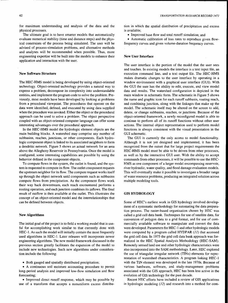
62

for maximum understanding · and analysis of the data and the physical processes.

The ultimate goal is to have smarter models that automatically evaluate numerical stability (time and distance steps) and the physical constraints of the process being simulated. The user will be advised of process-simulation problems, and alternative methods and analyses will be recommended when possible. Thus, more engineering expertise will be built into the models to enhance their application and interaction with the user.

New Software Structure

The HEC-HMS model is being developed by using object-oriented technology. Object-oriented technology provides a natural way to express a problem, decompose its complexity into understandable entities, and implement the program code to solve the problem. Previously, most models have been developed by looking at problems from a procedural viewpoint. The procedures that operate on the data were identified, defined, and executed by using data supplied when the procedure was invoked. Either the object or the procedural approach can be used to solve a problem. The object perspective coupled with an object-oriented computer language can offer some interesting advantages over the procedural approach.

In the HEC-HMS model the hydrologic element objects are the main building blocks. A watershed may comprise any number of subbasins, reaches, junctions, or other components. Each hydrologic component object is linked to its associated neighbors to form a dendritic network. Figure 5 shows an actual network for an area above the Allegheny Reservoir in Pennsylvania. Once the model is configured, some interesting capabilities are possible by using the behavior defined in the component objects.

To compute flows in the system, the outlet is found, and the system is requested to compute its flow. The outlet component requests the upstream neighbor for its flow. The compute request works itself up through the object network until components such as subbasins compute flows from precipitation. As the component flows work their way back downstream, each reach encountered performs a routing operation, and each junction combines its inflows. The final result of outflow is then available at the outlet. This illustrates the concept of an object-oriented model and the interrelationships that can be defined between objects.

New Algorithms

The initial goal of the project is to field a working model that is useful for accomplishing work similar to that currently done with HEC-1. As such the model will initially contain the most frequently used algorithms in HEC-1. Later releases will incorporate newer engineering algorithms. The new model framework discussed in the previous section greatly facilitates the expansion of the model to include new technologies. Such new algorithms under consideration include the following:

• Both gauged and spatially distributed precipitation; • A continuous soil moisture accounting procedure to permit

long-period analysis and improved low-flow simulation and flow forecasting;

• Improved direct runoff response, which may be possible by use of a transform that accepts a nonuniform excess distribu-


tion in which the spatial distribution of precipitation and excess is available;

• Improved base flow and total runoff simulation; and • Automatic calibration of loss rates to reproduce given flow

frequency curves and given volume-duration frequency curves.

New User Interface

The user interface is the portion of the model that the user sees and touches. In existing models the interface is a text input file, an execution command line, and a text output file. The HEC-HMS makes dramatic changes to the user interface by operating in a window environment with a graphical user interface (GUI). With the GUI the user has the ability to edit, execute, and view model data and results. The watershed configuration is depicted in the main window in schematic form. The schematic in Figure 5 shows the name and graphic icon for each runoff subbasin, routing reach, and combining junction, along with the linkages that make up the model. The schematic itself may be altered on the screen to add, delete, or change subbasins, reaches, or junctions. Because of the object-oriented framework, a newly reconfigured model is able to continue to perform all of its runoff functions without other user actions. The internal object representation used to perform model functions is always consistent with the visual presentation in the GUI schematic.

The GUI is currently the only access to model functionality. Although it is not yet designed and implemented, it has been recognized from the outset that for large project requirements the HEC-HMS model must be able to be driven from other processes, as well as by the interactive GUI user. With the ability to accept commands from other processes, it will be possible to use the HECHMS as one component of a larger model encompassing reservoir, river hydraulic, water quality, and flood damage evaluation models. This will eventually make it possible to investigate a broader range of water resource problems, producing an integrated solution across multiple modeling tools.

GIS HYDROLOGY

Some of HEC's earliest work in GIS hydrology involved development of a systematic methodology for automating the data preparation process. The raster-based organization chosen by HEC was called a grid cell data bank. Techniques for use of satellite data, for conversion of polygon data to a grid format, and for use of commercially available software to manipulate and convert the data were developed. Parameters for HEC-1 and other hydrologic models were computed by a program called HYDP AR (11) that accessed the grid cell data. In 1975 the grid cell data bank approach was formalized in the HEC Spatial Analysis Methodology (HEC-SAM). Remotely sensed land use and other hydrologic characteristics were also incorporated into the SAM methodology. Later, HEC explored the use of triangular irregular network (TINs) elements for representation of watershed characteristics. A program linking HEC-1 with the TIN element was developed in the late 1970s. Because of various hardware, software, and study-management problems associated with the GIS approach, HEC has been less active in the evolution of GIS technology for the past decade.

Recent HEC efforts have included a review of GIS applications in hydrologic modeling (12) and research into a method for com-

Name

DHorfpUon

Drainage Ana

Model Location

UpStr11m Name

UpStreamName

Downstream Name

Index Point

~ Reach

J~ Catchment

Gtogrephlc Location (opdonll)

Longitude (dlnllt)

l.ethud• (dlnlls),

Channel Cep1clty

OK " II Cancel

FIGURE S NexGen hydrologic modeling system.

.. a aa• llodellS.. 0...,-& .. ,.~ ---··--···--··· ------

_,, ... .,.._,,._ --- ~ .,.....,., ..... .. MITl• Old• DatetTlM

eae Ht IOot 1420, I..,.. .... " 141 HJ\lllH11200 eae Ut 1001 1tHl IUmHtt200 411 14.1\inlt I 1100 eat IU IOOO ltU IUllDlttHOO t1 l~HtltOO cat HI 1001 ,, .......... 11 ... IOI lt.ilmlltllOO llcla IU 1001 114, 11.llmlttllOO ... lt.ftmlt t 1400 C:.t Ill IOot Slot ILt'llDUtttot HI IU\mlttllOO .... 474 1001 IOI IUllDlhHM HI lu.lttllOO ,,.. Ill 1000 IOIN l&..Jldtallot 411 l&11elt1UOO .. IOl 1001 nu u ..... ttuoo 411 14.l\lllH t ISOO .rot IHO IOOO Uotl llJ\anlhlJIO 147 IUW.HtUOO .. UH IOOO HOl IUltnltattot ·u ::=:m:: , cae 100 1001 41111..,_.hlOOO 111111 100 1001 CHI IU'llDHtHOO 41 llJ\lnlttllOO .rot UH 100• &IHI ILIWllltlSOO JOH l..,_.ltUot .rot HSI IOot JOHI IMmllttHOO IHI IC.M\lttUOO .. HSI lOOI IOHI 10.llmllrHOO 1111 14'1111111Uot

... UH

JOSH IOUC

I rt:

I~: ~ ~:~ f

Ill:

11::~ I c:3 BE1.<M 0.0 t;;;

~~~~~::::~~::::~~~~~~~~~~-::::~::::~::::::::::::::::::~::::::::~:::::: ~::~d:~

64

bining the spatial GIS data with lineal hydrologic networks. A hybrid grid-network procedure for adapting these existing GIS capabilities for hydrologic modeling is being investigated. Spatially distributed processes are represented on a grid, and one-dimensional flow and transport occur through an associated network. There is a duality between a grid and a network in that once the direction of flow on each grid cell is defined to a single neighboring grid cell, an implied flow network is created. These ideas are being further investigated in HEC's NexGen and in remote-sensing and GIS projects.


CURRENT RESEARCH AND DEVELOPMENT ACTIVITIES

In fiscal year 1994 HEC will begin a new work unit for research and development into urban hydrology and hydraulics. Many more Corps flood control investigations are now being conducted in urban areas. Several simulation models exist in the profession to perform these analyses, but each has its particular purpose. Each of the models has limitations, too. The intent of this research is to

TABLE 1 HEC Urban Hydrology Capabilities and Needs

Existing Hypothetical frequency-based storms: Nested intensities balanced in time

Infiltration: Land use-based Lump sum computation No recovery during dry periods Impervious area

Drainage system: Typical collector system or detailed .simulation Two land-surface-runoff planes No inlet control or check on storm drain

capacity Collector channel routing

Channel routing: Several hydrologic methods Kinematic wave and Muskingum-Cunge for

typical urban channels Muskingum-Cunge widely applicable No storm sewer hydraulics except via data

storage system

Diversions: Single monotonic function

Pumping stations: Fixed computation time interval causes

oscillations between "on" and "off' times

Detention storage: Level pool reservoir routing Culvert outflow submerged

Water quality: Only STORM computes land surface runoff

quality

Project analysis: Fixed channel sires Modified flow-frequency curves Flood damage calculation Multi-flood and multi-project simulation

Needed

Other hypothetical storm distributions

Replacement for SCS Curve Number Distribute in time while water is on plane Soil moisture accounting OK

OK OK Check for inlet control and storm drain

capacity Test diffusion routing in collectors

Additional checks for stability of computation Check for channel capacity and limit flow.

Test diffusion routing for improvements More direct connection of HEC-1 to unsteady

flow model UNET or SWMM EXTRAN

More flexible function with changes based on time and stage

Dynamic time interval

OK Include free surface and pressure flow

Add water quality routing or connect through data storage system

Automatic storm drain sizing Automatic calibration to frequency curve OK OK

Feldman

review the needs of Corps field offices, understand the limitations of existing models, develop guidance for the use of existing models for different types of investigations, and develop new or modified models as necessary to meet the needs. Table 1 summarizes the present status and perceived needs for urban hydrologic modeling capabilities at HEC.

One of the areas of concern is the transition from surface runoff to storm sewer flow. Inadequate inlet capacity and surcharging storm sewers make the simulation difficult. The SWMM EXTRAN module addresses this problem, but it has limitations. One consideration will be to use HEC's new unsteady-flow routing program, UNET (13), to perform the storm sewer routing. UNET has the capability of simulating flow in looped networks under free-surface and pressure-flow conditions. It presently interacts with HEC-DSS for input and output. UNET will have to be tested in such urban applications in conjunction with HEC-1. A dynamic link between the two models may be desirable.

CONCLUSIONS

Several existing and emerging software packages for urban hydrologic modeling and analysis have been presented. More detailed information on any of the capabilities can be obtained from HEC. The purpose of HEC software is to help solve hydrologic analysis problems faced by Corps field offices. HEC follows a very applications-oriented approach to software development and problem solving. The development of new urban hydrology software will follow this same approach. One of the first tasks in the new research and development work unit will be to host a seminar to bring Corps users in contact with leaders in the urban hydrology profession. It will serve to both apprise the profession of the Corps's needs and review the latest capabilities of the profession. With that information in hand, new and modified methods, models, and guidance will be developed. The result will be a set of physically based models with applications guidance that can be used to solve urban hydrology problems in gauged and ungauged areas.

65

REFERENCES

1. Feldman, A. D. HEC Models for Water Resources System Simulation: Theory and Experience. Advances in Hydroscience (V. T. Chow, ed.), Vol. 12, 1981, pp. 297-423.

2. Flood Damage Analysis Package, User's Manual. Computer Program Document 59. Hydrologic Engineering Center, U.S. Army Corps of Engineers, Davis, Calif., 1988.

3. HEC-1 Flood Hydro graph Package, User's Manual. Computer ·Program Document IA. Hydrologic Engineering Center, U.S. Army Corps of Engineers, Davis, Calif., 1990.

4. Introduction and Application of Kinematic Wave Routing Techniques Using HEC-1. Training Document 10. Hydrologic Engineering Center, U.S. Army Corps of Engineers, Davis, Calif., 1979 (updated in 1993).

5. Garbrecht, J., and G. Brunner. Hydrologic Channel-Flow Routing for Compound Sections. Journal of Hydraulic Engineering, ASCE, Vol. 117, No. 5, 1991, pp. 629-642.

6. Davis, D. W. Optimal Sizing of Urban Flood-Control Systems. Journal of Hydraulic Engineering, ASCE, Vol. 101, No. HY8, Aug. 1975, pp. 1077-1092.

7. HEC-1FH Interior Flood Hydrology, User's Manual. Computer Program Document 31. Hydrologic Engineering Center, U.S. Army Corps of Engineers, Davis, Calif., 1992.

8. STORM Storage, Treatment, Overflow, Runoff Model, User's Manual. Computer Program Document 7. Hydrologic Engineering Center, U.S. Army Corps of Engineers, Davis, Calif., 1977.

9. HEC-DSS Data Storage System, User's Guide and Utility Program Manuals. Computer Program Document 45. Hydrologic Engineering Center, U.S. Army Corps of Engineers, Davis, Calif., 1990.

10. Huber, W. C., and R. E. Dickinson. Storm Water Management Model, Version 4: User's Manual. Environmental Research Laboratory, Environmental Protection Agency, Athens, Ga., 1988.

11. HYDPAR Hydrologic Parameters, User's Manual. Computer Program Document 34, Hydrologic Engineering Center, U.S. Army Corps of Engineers, Davis, Calif., 1985.

12. DeVantier, B. A., and A. D. Feldman. Review of GIS Applications in Hydrologic Modeling. Journal of Water Resources Planning and Management, ASCE, Vol. 119, No. 2, March-April 1993, pp. 246-261.

13. UNET One-Dimensional Unsteady Flow Through a Full Network of Open Channels, User's Manual. Computer Program Document 66. Hydrologic Engineering Center, U.S. Army Corps of Engineers, Davis, Calif., 1993.



Scour Around Wide Piers in Shallow Water

PEGGY A. JOHNSON AND EDUARDO F. TORRICO

The assessment of pier scour at many bridges is a difficult task because of the numerous complexities of the scour process. One of these complexities occurs when the flow depth is shallow ~elati~e t? the pier width. A preliminary examination of the effect of wide piers m shallow water is provided and a modification or correction factor for currently used scour equations to account for this effect is developed. An experiment was conducted to test the effect of shallow flow depths and wide piers while keeping all other variables constant. Existing laboratory data along with data from the study were analyzed to incorporate the effects of wide piers on the scour at bridge piers. During the study regions of relative flow depth (flow depth-to-pier width ratio) at which the scour process differs were determined. The definitions of wide piers a~d shallow flow in terms of the relative depth to pier width were established.

Engineers across the United States assess scour conditions at existing bridges and determine the need for scour mitigation. The assessment of scour at many bridges is a difficult task because of the numerous complexities of the scour process, one of which occurs when the flow depth is shallow relative to the pier width. In addition, the Froude number upstream of the bridge may be quite low, a condition for which current scour equations do not account. These conditions exist at many bridges in coastal areas. Two examples in Maryland are the Severn River and Woodrow Wilson bridges. At the Severn River Bridge, for example, 8 of the 12 piers have widths that exceed the flow depth. The ratios of flow depth to pier width range from 0.18 to 0.86. The Froude numbers at these piers, even for a large storm event, are quite low (about 0.2 or less). At inland bridges the flow depth may be very shallow relative to an exposed pier foundation. At these coastal and inland bridges it is often noted by engineers that the scour equations recommended by FHW A (J) yield excessively large scour depths.

In studies conducted at the University of Auckland (2), the effect of flow depth on scour for shallow water conditions was recognized. To account for this condition, Melville and Sutherland (2) recommended a multiplicative factor when the ratio of flow depth to pier width is less than 2.6. Although this factor yields lower scour depths compared with those from HEC-18 estimates, the estimates are still quite high relative to observed scour depths in the field.

The objective of the present study was to provide a preliminary examination of the effect of wide piers in shallow water and to develop a modification or correction factor for currently used scour equations to account for this effect.

LOCAL SCOUR AT WIDE PIERS IN SHALLOW WATER

Local scour can be caused by an obstruction, such as a bridge pier or abutment, in the stream flow. Although many parameters affect local scour (3,4), the present study concentrated on three parameters: pier size, flow depth, and velocity.

Department of Civil Engineering, University of Maryland, College Park, Md. 20742.

It is generally accepted by researchers [e.g., Laursen and Toch (5), Laursen (6), and Neill (7)] that relative scour depth (ys lb, where Ys is scour depth and bis pier width) increases as the relative flow depth (y/b, where y is flow depth) increases until a certain limiting value of y/b is reached, after which the relative scour depth is independent of ylb. The limit expressed by most researchers is in the range of 1 < ylb < 3. Flow depth affects both clear-water and livebed scour depths. When considering the effect of flow depth on local scour depth, it is essential that all other variables affecting pier scour, especially pier size and sediment size, be held constant. To keep the effect of velocity on scour depth constant, the velocity ratio (VIVc, where V is the stream flow velocity and Ve is the critical velocity) needs to be kept constant (e.g., at incipient motion).

For clear-water scour, Bonasoundas (8) concluded that the effects of flow depth became insignificant for y/b > 1 to 3. Ettema (9) stated that the influence of flow depth is affected by the relative size of the pier and sediment. He concluded that for high values of bldso (typical of a prototype setting), the development of local scour is almost independent of flow depths for ylb > 1, whereas for low values of bld50 (typical of a laboratory setting), scour depth is still dependent on flow depths even when the value of ylb is as high as 6. Ettema (9) stated three reasons that account for the reduction in equilibrium scour depths for shallow flows. First, the portion of the approach flow available to be diverted into the scour hole diminishes for low values of y/b. Second, the development of the scour hole is influenced by the formation of a sediment bar behind the pier for low values of y/b. Third, the formation of a surface roller, on a bow wave that has a sense of rotation opposite that of the horseshoe vortex at the free surface around the pier, interferes with the horseshoe vortex and the down flow into the scour hole. Ettema (9) further added that a ylb value equal to 3 was especially significant for coarse sediment.

Basak (10), Jain and Fischer (11), and Chee (12) showed that flow depth has an effect on live-bed scour similar to that on clear-water scour in which scour depth is lower for decreasing values of y/b.

EXISTING MODELS FOR PREDICTING SCOUR DEPTH

The Hydraulic Engineering Circular 18 (HEC-18) equation is recommended by FHW A (J) to estimate both live-bed and clear-water pier scour depths. The equation predicts maximum pier scour depths as follows:

where

y s = scour depth, y =flow depth,

(1)

Johnson and Torrico

K1 = correction factor for pier nose shape, K2 = correction factor for angle of attack of flow, K3 = correction factor for bed condition, b = pier size, y = flow depth, and F = Froude number.

Equation 1 applies only to subcritical flow. For circular piers, Equation 1 reduces to

(2)

The University of Auckland pier scour equation (J) is based on a set of corrective factors based on laboratory data:

where

K1 = correction factor for the flow intensity, Ky = correction factor for the flow depth, Kd = correction factor for the sediment size, K:r = correction factor for sediment gradation, and

(3)

Ks, Ka = correction · factors for pier shape and alignment, respectively.

For circular piers and uniform sediment sizes of b/d50 of more than 50, Equation 3 reduces to

Ys = KK b I y (4)

Ky accounts for wide piers and shallow flow depths. Melville and Sutherland (2) determined the following equation for Ky on the basis of laboratory experimentation:

- (..t)0.255 Ky - 0.78 b for y/b < 2.6 (5)

for ylb :2:: 2.6

EXPERIMENTAL PROGRAM

A set of experiments was conducted to further determine the effect of wide piers in shallow water on scour depth. The effects of various values of flow depth to pier width ratios (ylb) on scour depth were studied by systematically varying the pier size and the flow depth. During the experiment a uniform sediment (d50 = 0.93 mm) was used with a b/d50 of >50 to avoid the influence of sediment size on scour depth. All runs were conducted at approximately incipient motion velocity to represent maximum scour conditions. Only subcritical flow and circular piers were used. In this manner only the effects of the pier size and the flow depth on scour were studied.

The ranges of ylb studied were selected on the basis of the corrective factors of ylb between 0 and 2.6 suggested by Melville and Sutherland (2). Within this range the effects of pier size and flow depth are most noticeable. A few experimental runs of y/b between 2.6 and 5 were conducted to observe the limiting value of y/b at

67

which the flow depth no longer influences the scour depth. The experiments were conducted at the FHW A Hydraulics Laboratory at the Turner-Fairbank Research Center in McLean, Virginia. All of the experiments were conducted in a 1.8-m-wide, 21.3-m-long, glass-walled tilting flume. The flume had a fixed bed except for a 1.8-m-wide, 1.2-m-long, 0.46-m-deep observation area located approximately in the center of the flume. The bed upstream of the observation area was covered with a 5-cm layer of sand to stabilize the approach velocity and shear stress of the bed at the observation area. Five models with various pier diameters were used to ensure an adequate range of y/b values. Model bridge piers constructed from 6-, 9-, 11-, 16-, and 25-cm (outside diameter) polyvinylchloride pipes were used. Each pipe was bolted to a square wooden plate by an o-ring plastic joint and was placed on the floor in the center of the flume observation area.

To avoid side-wall effects on scour, the circular pier sizes used in the experiment were close to the recommended values for the pier width-to-flume width ratio by Chiew (13) of 1/10 and Shen et al. (14) of 1/s. The 1/10 and 1/s ratios were established to ensure that no contraction scour was present as a consequence of decreasing the flow area by the pier width; thus, all scour was local only. However, during the experiment it was observed that the limiting value for pier width-to-flume width ratio is highly dependent on the flow depth. Thus, the pier width-to-flume width ratios can be reduced even further for shallow flow experiments.

RESULTS AND DISCUSSION OF RESULTS

The results of the experiments collected during the 23 runs are given in Table 1. There was very little variation in velocity since d50 was constant and VIVc was kept at approximately 1. Relative flow depths varied from 0.25 :::; ylb:::; 5.0. Resulting scour depths ranged from 8 to 21 cm.

Effect of Pier Size

Scour depth versus pier size is plotted in Figure 1 using the experimental data. Melville and Sutherland (2) found that the ratio of scour depth and pier size, ysfb, reaches a maximum of 2.3 at y/b of about 2.6. The line of 2.3 times the pier size was plotted in Figure 1 to show that the 2.3 limiting value applies mostly to small piers, where the ratio of y/b is usually >2.6. The line of 2.3 grossly overestimates the scour depth for larger pier sizes. The influence of flow depth on scour depth is shown as the variation between the upper and the lower values of scour obtained for the different pier sizes used in the experiment (Figure 1). The upper values represent deep flows. The closeness of the points at deep flows indicates that the influence of the flow depth is diminished. The lower values of scour represent shallow flows. At shallow flows the points are more separated, indicating that the flow depth has a greater influence on scour depth.

In summary, pier size has a direct relationship with scour depth: the larger the pier size, the deeper the scour depth. However, the data show that for small piers the influence of pier size is greater than that for large piers (Figure 1). Also, the value of Ys lb equal to 2.3 as established by previous researchers is only applicable to small piers, where the influence of the flow depth is diminished considerably.

68

TABLE 1 .Experimental Data

Pier Flow Velocity Width Depth

Run# (mis) (cm) (cm)

1 0.482 16.8 5.2 2 0.457 16.8 6.6 3 0.456 16.8 8.5 4 0.512 16.8 11.9 5 0.468 16.8 15.2 6 0.464 16.8 16.7 7 0.482 16.8 21.8 8 0.482 16.8 25.2 9 0.477 16.8 28.5 10 0.455 16.8 33.6 11 0.468 6.0 6.0

11-A 0.480 6.0 9.2 12 0.455 6.0 12.1 13 0.475 6.0 18.1 14 0.488 6.0 24.1 15 0.482 6.0 30.2 16 0.458 11.4 5.7 17 0.455 11.4 11.4 18 0.492 11.4 22.9

18-A 0.484 11.4 34.3 19 0.484 11.4 28.5 20 0.476 8.9 28.5 21 0.485 8.9 8.9 22 0.487 25.4 26.4 23 .0.467 25.4 6.5

Effect of Flow Depth

The laboratory results of scour depth and flow depth are plotted in Figure 2. Scour depth has a direct relationship with flow depth. The influence of flow depth on scour depth diminishes as the flow depth increases (Figure 2). At higher flow depths there is a maximum at which flow depth no longer influences scour depth; instead, it is influenced primarily by pier size. Thus, for each pier size there is a maximum flow depth at which scour depth is influenced by pier size alone (in the absence of other factors). At lower flow depths the importance of pier size decreases and the flow depth becomes more influential on scour depth. The results agree with the analysis whose results are shown in Figure 1.

0.35

0.3 >-

:§: 0.25 0

~ Deep.nows '),· .s::. Q

~ 0.. 0.2 r -<' Q)

8 0

C:o.15>-

* + ::I + 0 0.1 ~ * Shallow flows (.)

en 0.05

00 0.05 0.1 0.15 0.2 0.25 0.3 Pier Size b (m)

FIGURE 1 Experimental results of scour depth as function of pier width.

Ve (mis)

0.38 0.40 0.41 0.44 0.45 0.46 0.48 0.49 0.50 0.52 0.39 0.42 0.44 0.47 0.49 0.51 0.39 0.43 0.49 0.52 0.50 0.50 0.42 0.50 0.39


Scour Depth

V/Vc F y/b (cm)

1.27 0.68 0.31 14.6 1.16 0.57 0.39 15.3 1.11 0.50 0.50 17.1 1.17 0.47 0.71 17.5 1.03 0.38 0.90 19.8 1.01 0.36 0.99 20.4 1.00 0.33 1.30 20.8 0.98 0.31 1.50 20.9 0.95 0.29 1.70 21.0 0.88 0.25 2.00 21.0 1.20 0.61 1.00 8.0 1.15 0.51 1.53 9.3 1.04 0.42 2.00 9.0 1.02 0.36 3.00 10.3 0.99 0.32 4.00 9.8 0.95 0.28 5.00 10.8 1.19 0.61 0.50 11.7 1.05 0.43 1.00 14.5 1.01 0.33 2.00 16.1 0.93 0.26 3.00 16.3 0.96 0.29 2.50 16.2 0.94 0.28 3.21 13.3 1.17 0.52 1.00 11.0 0.98 0.30 1.04 27.7 1.19 0.59 0.25 18.5

Effect of Velocity

The depth of the local scour hole is closely related to the approach flow velocity for clear-water conditions. It was shown by Chabert and Engeldinger (15), Ettema (9), and Chiew (13) that under clearwater conditions y/b increases almost linearly as VIVc increases from 0 to 1, reaching a maximum when VIVc is nearly equal to 1.

The variation of the velocity during the experiment was minimal, as seen in Table 1. This is because the incipient motion velocities for the size of sediment used in the experiment do not vary significantly with flow depth. For this reason no conclusions can be drawn about the velocity by using the laboratory data. Data from other studies along with the data from the present experiment (all sub-

0.3

0.25

]:

= 0.2 c. o. Q) • c

,,. ~ 0.15 ~ • 0 c.> fl) • 0 0.1 •• • •

0.05 0 0.1

() b=025m

• • • • •

0

• • 0.2 0.3 Flow Depth (m)

b=0.17m

• b=0.11 m

b= 0.09m

b = 0.06 m

0.4 0.5

FIGURE 2 Experimental results of scour depth as function of flow depth.

Johnson and Torrico

critical flow) for an approximate 15-cm pier size were analyzed· to account for the effect of velocity on scour depth. The results are shown in Figure 3. The plot shows that the scour depth increases as the velocity increases until a maximum is reached, after which the scour depth is independent of velocity. It is important to mention that there is a slight decrease in scour depth after incipient motion is reached. The decrease of scour depth at high velocities has been attributed to bed forms (J 3). The Froude number can be used to describe the velocity effect on scour depth, although it should be recognized that the Froude number is also a function of flow depth. Therefore, variation in scour depth with changes in Froude number may be caused by either velocity or flow depth.

Effect of Flow Depth-to-Pier Width Ratio

Pier size and flow depth have been shown to affect pier scour. This effect can be analyzed further through the use of ratios. Dimensionless laboratory ratios are frequently used in pier scour engineering as a way to scale from laboratory results to prototype sizes.

Data from Chiew (13), Colorado State University (CSU) (16), Chabert and Engeldinger (15), Hancu (17), Jain and Fischer (JJ), Shen et al. (14), Y anmaz and Altinbilek (18), and the present study are plotted in Figure 4 as Ys lb versus ylb for bld50 of >50 and for Froude numbers of <0.7. These data represent both clear-water and live-bed conditions. It was shown by Chiew (13) that for a bld50 of >50 the influence of ylb on scour depth for live-bed conditions is about the same as that for clear-water conditions. From Figure 4 it is apparent that the relative scour depth increases with relative flow depth at a decreasing rate and that there is a limiting relative flow

0.25 ,...------------------------.

0.2

g = 0.15 Q. G)

c 5 0 1 ~ 8 . en

0.05

0.2 0.4

EB

ffi <> <> EB

0.6 0.8 1.2 Flow Velocity (mis)

FIGURE 3 Laboratory data showing scour depth as function of velocity.

2.5

~ ~ 2 = "C .

~ lii 1.5 c::: 0 - 1 a G)

c 5 0.5 8 en

0 °*@ 0

~.: • 0

. -~ 0

0 .. ~ . 0

~·-- • ·' ~ 8 .·' . * . . .

* 2 4 6 Flow Depth to Pier Width (y/b)

Chiew(13) 0

CSU!16J

• Chabert (15) • • Hancu (171

D Jain & Fischer (11)

<> Shen et al. (14)

* Yanmaz {18J . This study

8

FIGURE 4 Relative scour depth as function of relative flow depth.

3

~ ~2.5

a ~ 2

~ u:: 1.5

a1 G)

c 5 0.5 8 en

. i···

*'o~* ,.t-80 ••

* 2 3 Pier Width to Flow Depth (b/y)

69

Chlew(13) . CSUt16J

• Chal>ert(15)

• Hancut17J

D Jain end Fiscller(11)

<> Shen et al. (14)

* Yanmaz (181 0

This study

5

FIGURE 5 Relative scour depth as function of relative pier width.

depth beyond which the reiative scour depth is unaffected by flow depth. It is also apparent that the scour depth is mostly independent of relative flow depth at the limiting ylb value of 2.6 (2), at which the scour depth is largely influenced by the pier size. The limiting value of Ys lb of 2.3 indicates the maximum relative scour depth to pier width (Figure 4).

Using the same data, YslY versus bly is plotted in Figure 5. It shows that the relative scour depth increases with pier size at a decreasing rate and that there is a limiting pier size beyond which the scour depth is mostly unaffected by the relative pier size.

DEVELOPMENT OF CORRECTION FACTOR FOR WIDE PIERS

FHW A recommends the use of Equation 1 for estimating maximum scour at a pier. This equation was developed for a ylb value of ;:::: 0.8. As shown in the previous sections the process for wide piers in shallow flows differs from that in deeper flows; therefore, extrapolation of Equation 1 to values of ylb of :::; 0.8 may result in overprediction. The process also differs depending on whether VIVc is greater than or less than 1.

Two correction factors were developed for Equation 1 for wide piers in shallow flow (i.e., ylb < 0.8), depending on the value of VIVn using data from the present study and the other studies mentioned in the previous section. To develop the correction faetors, two equations were calibrated in a manner similar to that for the format of Equation 1. For ylb of< 0.8 and VIVc of < 1, only nine sample points were available. This is a very small sample set from which to calibrate three coefficients, and the results should be regarded as preliminary. A sample set of 21 datum points was used for VIVc of ;:::: 1. The calibration yielded the following equation:

Ys = 5.16 (!z_)o.31p1.os y . y

for VIVc > 1 (6a)

for VIVc ;:::: 1 (6b)

Equations 6a and 6b were calibrated by a nonlinear, least-squares optimization. Problems in creating bias and spurious correlations were avoided by calibrating the equations for Ys and holding the coefficient of y at 1. For Equation 6a R2 was 0. 97, and for Equation 6b R2 was 0.99.

From Equations 6a and 6b correction factors for Equation 1 were developed by dividing Equations 6a and 6b by Equation 1 to yield the following:

70

( Y

)0.34

K = 2.58 b F0·65 for VIVc < 1 (7a)

( v )0.13

K = 1.0 b Fo.20 for VIVc ~ 1 (7b)

It is worth repeating that the correction factors of Equations 7a and 7b are for y/b of <0.8 only and are developed to correct Equation 1.

To illustrate the use of the correction factors developed in Equations 7a and 7b, the Severn River Bridge in Maryland is used as an example. This bridge has 12 piers withy/b values ranging from 0.17 to 1.88. For Pier 1, ylb is 0.18, Fis 0.19, andy is 1.1. By using Equation 1, Ys is equal to 3.57 m. From Equation 7a, K is equal to 0.49. The adjusted scour depth is 3.57(0.49) = 1.75 m. This is a squarenosed footing, so multiplying by 1.1 yields a final scour depth of 1.93 m. At another pier at this same bridge, y/b is 0.68, Fis 0.1, and y is 5.24 m. Equation 1 yields a scour depth of 4.27 m. The correction factor K, from Equation 7a, yields 0.51, producing an adjusted scour depth of 0.51 ( 4.27) = 2.16 m.

The Woodrow Wilson Bridge across the Potomac River in Maryland also has several wide piers. As an example, at one of the piers y/b is 0.73 and Fis 0.26. Equation 1 for this pier provides an estimated scour depth of 1.68 m. Use of Equation 7b yields a correction factor of 0.73, producing an adjusted scour depth of 1.22 m.

LIMITATIONS OF CORRECTION FACTORS

Several limitations of the correction factors developed here should be noted. The correction factors apply only for subcritical flows aild uniform noncohesive sediments with b/d50 of >50. The correction factors were developed only for ylb values of <0.8 and for both live-bed and clear-water conditions; the f~ctors should be limited to use under these conditions. Extrapolation to values outside the range of data used in the calibration could result in inappropriate values of scour.

The correction factors developed in the present study are only preliminary results. Equation 6a was based on a limited number of datum points and should be recalibrated when more data become available. In addition, the Froude numbers associated with wide piers in shallow water are often quite small. The Froude numbers used in the calibration of Equations 6a and 6b were not less than about 0.2; therefore, care should be taken in using the correction factors for extremely low Froude numbers.

CONCLUSIONS

This preliminary study on scour at wide piers has demonstrated the differences in scour processes at wide piers in shallow water. Correction factors were developed for use with the HEC-18 equation (Equation 1). These factors reduce the amount of scour for wide piers in shallow water. Although previous studies have also demonstrated the reduction of scour at wide piers, this information was not readily usable with the HEC-18 equation. Use of the correction factors can assist in estimating scour at bridges, particularly in coastal areas where pier widths tend to be shallow relative to flow depths.

The preliminary results provided here could be improved by conducting additional experiments to produce larger sample sizes from

TRANSPORTATION RESEARCH RECORD ]471

which to calibrate the equations. Experiments should also be conducted to examine the process of scour at very low Froude numbers (less than about 0.25). These data could then be used with the wide pier data to develop a method or correction factors to estimate the scour in tidal areas. In addition, field verification of the correction factors would be of value.

ACKNOWLEDGMENTS

The authors gratefully acknowledge the valuable comments and discussions of Sterling Jones and Stanley Davis as well as the technical assistance provided by David Bertoldi and Edward Umbrell during the laboratory experiment at the FHW A laboratory in McLean, Virginia.

REFERENCES

1. Evaluating Scour at Bridges: HEC 18, 2nd ed. FHWA-IP-90-017. FHW A, U.S. Department of Transportation, April 1993.

2. Melville, B. W., and A. J. Sutherland. Design Method for Local Scour at Bridge Piers. Journal of Hydraulic Engineering, ASCE, Vol. 114, No. 10, 1983,pp. 1210-1226.

3. Breusers, H. N., G. Nicollet, and H. W. Shen. Local Scour Around Cylindrical Piers. Journal of Hydraulic Research, Vol. 15, No. 3, 1977, pp. 211-252.

4. Jain, B. P., and P. N. Modi. Comparative Study of Various Formulae on Scour Around Bridge Piers. Journal of the Institute of Engineering (India), Vol. 67, Part Cl 3, 1986, pp. 149-159.

5. Laursen, E. M., and A. Toch. Model Studies of Scour Around Bridge Piers and Abutments-Second Progress Report. HRB Proc., Vol. 31, 1956, pp. 82-87.

6. Laursen, E. M. Bridge Design Considering Scour and Risk. Journal of Transportation Engineering, ASCE, Vol. 96, No. TE2, 1970, pp. 149-164.

7. Neill, C.R. Guide to Bridge Hydraulics. Roads and Transportation Association of Canada, University of Toronto Press, Canada, 1973.

8. Bonasoundas, M. Non-Stationary Hydromorphological Phenomena and Modelling of Scour Processes. Proc., 16th Congress of the International Association of Hydraulic Research, Sao Paulo, Brazil, Vol. 2, 1973, pp. 9-16.

9. Ettema, R. Scour at Bridge Piers. Report 216. School of Engineering, University of Auckland, 1980.

10. Basak, V. Scour at Square Piers (Devlet su isteri genel mudulugu). Report 583. Ankara, Turkey, 1975.

11. Jain, S. C., and E. E. Fischer. Scour Around Circular Bridge Piers at High Froude Numbers. Report FHWA-RD-79-104. FHWA, U.S. Department of Transportation, 1979.

12. Chee, R. K. W. Live-Bed Scour at Bridge Piers. Report 290. School of Engineering, University of Auckland, 1972.

13. Chiew, Y. M. Local Scour at Bridge Piers. Report 355. School of Engineering, University of Auckland, 1984.

14. Shen, H. W., Y. Ogawa, and S. Karaki. Local Scour Around Bridge Piers. Journal. of Hydrology, ASCE, Vol. 95, No. HY6, 1969, pp. 1919-1939.

15. Chabert, J., and P. Engeldinger. 1956. Etude des Affouillements Autour des Piles de Ponts. Laboratoire National d'Hydrologie, Chatou, France, Oct. 1956.

16. Mechanics of Local Scour. Colorado State University. Fort Collins; Bureau of Public Roads, U.S. Department of Commerce, 1966.

17. Hancu, S. Sur le Calcul des Affouillements Locaux dans la Zone des Piles de Pont. Proc., 14th Congress of the International Association of Hydraulic Research, Vol. 3, 1971, pp. 299-306.

18. Yanmaz, M., and D. Altinbilek. Study of Time-Dependent Local-Scour Around Bridge Piers. Journal of Hydraulic Engineering, ASCE, Vol. 117, No. 10, 1991, pp. 1247-1268.


transportation research recordonlinepubs.trb.org/onlinepubs/trr/1994/1471/1471.pdf · sponsorship...

Documents