Transportation Resource Management

Sumit KunnumkalIndian School of Business, Gachibowli, Hyderabad, 500032, India

sumit kunnumkal@isb.edu

Huseyin TopalogluSchool of Operations Research and Information Engineering,

Cornell University, Ithaca, New York 14853, USAtopaloglu@orie.cornell.edu

February 23, 2010

Abstract

In this chapter, we describe a variety of modeling and solution approaches for transportation resourcemanagement problems. The solution approaches that we propose either build on deterministiclinear programming formulations, or formulate the problem as a dynamic program and usetractable approximations to the value functions. We describe two classes of methods to constructapproximations to the value functions. The first class of methods relax certain constraints in thedynamic programming formulation of the problem by associating Lagrange multipliers with them, inwhich case, we can solve the relaxed dynamic program by concentrating on one location at a time. Thesecond class of methods use a stochastic approximation idea along with sampled trajectories of thesystem to iteratively update and improve the value function approximations. After describing severalsolution approaches, we provide a flexible paradigm that is useful for modeling and communicatingcomplex resource management problems. Our numerical experiments demonstrate the benefits fromusing models that explicitly address the randomness in resource management problems.

Many problems in transportation logistics involve managing a set of resources to satisfy the servicerequests that arrive randomly over time. For example, truckload carriers decide which load requeststhey should accept and to which locations they should reposition the empty vehicles. Railroad companiesdeploy the empty railcars to different stations in the network to serve the random customer demand inthe most effective manner. Irrespective of the application setting, transportation resource managementproblems pose significant challenges. To begin with, these problems tend to be large in scale, spanningtransportation networks with hundreds of locations and planning horizons with hundreds of timeperiods. Furthermore, the service requests arrive randomly, and we may not have full informationabout the future service requests. When making the decisions for the current time period, we needto keep a balance between maximizing the immediate profits and getting the vehicles into favorablepositions to serve the potential future service requests. Finally, the decisions that we make for differentlocations and for different time periods interact in a nontrivial fashion. For example, the decision toserve a particular load from location i to j at time period t affects what other loads we can serve at thefuture time periods, since the vehicle that is used to serve the load at time period t becomes availableat location j at a future time period.

In this chapter, we describe a variety of modeling and algorithmic approaches for transportationresource management problems under uncertainty. We begin with a problem that takes place over twotime stages. At the first stage, we decide to which locations we should reposition the resources toserve the demands that arrive later. At the second stage, we observe the demand arrivals and decidewhich of these demands we should serve. The first algorithmic strategy that we discuss for the two-stage problem is based on a deterministic linear programming formulation. This formulation is simpleto implement, but it does not explicitly address the randomness in the demand arrivals. Motivatedby this observation, we move on to other algorithmic strategies that address the randomness in thedemand arrivals by using a dynamic programming formulation. The dynamic programming formulationof the two-stage problem turns out to be computationally difficult as it involves a high dimensional statevariable, and we resort to approximation strategies. In particular, the first two approximation strategiesthat we describe decompose the dynamic programming formulation by the locations and obtain goodsolutions by focusing on one location at a time. We also discuss a third approximation strategy thatconstructs separable value function approximations by using sampled trajectories of the system. Afterthe discussion of two-stage problems, we move on to resource management problems that take placeover multiple time periods. We give a dynamic programming formulation for a multi-stage resourcemanagement problem and demonstrate that the algorithmic concepts that we develop for two-stageproblems can be extended to multi-stage problems without too much difficulty.

In addition to providing algorithmic tools for two-stage and multi-stage problems, we also dwell onmodeling issues. Most transportation resource management problems involve complex resources. Forexample, a driver resource in a driver scheduling application may require keeping track of its inboundlocation, time to reach the inbound location, duty time within the shift, days away from home, vehicletype and home domicile. It would be cumbersome to model such complex entities through traditionalmathematical programming tools, and we provide a flexible paradigm that is useful for modeling andcommunicating complex resource management problems. We conclude the chapter with a series of

2

numerical experiments that demonstrate the benefits from using models that explicitly capture therandomness in the system.

Transportation resource management models have a long history dating back to the earliest daysof linear programming; see Dantzig and Fulkerson (1954), Ferguson and Dantzig (1955), White andBomberault (1969) and White (1972). The early models formulate the problem over a state timenetwork. The nodes of the state time network represent the supply of resources at different locationsand at different time periods, whereas the arcs represent the movements of the resources betweendifferent locations. These models tend to ignore the randomness in the problem and simply work withthe expected values of the demand arrivals. A subclass of the deterministic models is the so calledmyopic models, which ignore the unknown future altogether and only work with what is known withcertainty; see Powell (1988), Powell (1996) and Erera, Karacik and Savelsbergh (2008). This approachis justified by the fact that many customers call in advance, and a large portion of the future demandsis actually known with certainty. Whether they ignore the uncertainty in the future altogether orincorporate it through expectations of the demand arrivals, these kinds of deterministic models canyield tractable optimization problems and can be relatively simple to implement. As a result, they formthe backbone of many commercial systems; see Hane, Barnhart, Johnson, Marsten, Nemhauser andSigismondi (1995), Holmberg, Joborn and Lundgren (1998) and Gorman (2001).

The majority of the models that we discuss in this chapter fall under the category of stochasticmodels, which try to capture the random demand arrivals by formulating the problem as a dynamicprogram and using value functions to assess the impact of the current decisions on the future evolutionof the system. The dynamic programming formulations of practical resource management problemsgenerally involve high dimensional state variables, and this high dimensionality makes it impossibleto compute the value functions by using standard Markov decision process tools. Therefore, mostof the effort is concentrated around approximating the value functions in a tractable fashion; seeFrantzeskakis and Powell (1990), Crainic, Gendreau and Dejax (1993), Carvalho and Powell (2000),Godfrey and Powell (2002a), Godfrey and Powell (2002b), Kleywegt, Nori and Savelsbergh (2002),Adelman (2004), Topaloglu and Powell (2006), Adelman (2007) and Schenk and Klabjan (2008). Theoverview of transportation resource management models that we give in this chapter is rather compact,and it mostly evolves around methods that approximate the value functions. We refer the reader toPowell, Jaillet and Odoni (1995), Powell and Topaloglu (2005) and Barnhart and Laporte (2006) fordetailed reviews of deterministic and stochastic models. We also emphasize that our goal in this chapteris to give an overview of transportation resource management models in the literature, rather than tomake original contributions. At the end of each section in this chapter, we give pointers to the relevantliterature and acknowledge the original contributors.

The chapter is organized as follows. In Section 1, we formulate a two-stage resource managementproblem as a dynamic program. This formulation has a high dimensional state variable and we discussa variety of algorithmic approaches to obtain tractable approximations. In Section 2, we extend theideas that we discuss in Section 1 to multi-stage problems. In Section 3, we give a flexible paradigm formodeling complex resource management problems. In Section 4, we present numerical experiments.

3

1 Two-Stage Problems

In this section, we consider a resource management problem that takes place over a planning horizon oftwo time periods. Our goal is to illustrate the fundamental algorithmic concepts by using a relativelysimple problem setting. It turns out that all of the development in this section can be extended tomulti-stage problems without too much difficulty.

We have a set of resources that can be used over a planning horizon of two time periods to servethe demands that arrive randomly into the system. At the beginning of the first time period, thereis a certain number of resources at different locations. The decisions that we make at the first timeperiod involve repositioning the resources between different locations so that the resources end up atfavorable locations to serve the demands that arrive at the second time period. At the beginning ofthe second time period, we observe the demand arrivals. The decisions that we make at the secondtime period involve serving the demands by using the resources. The objective is to maximize the totalexpected profit over the two time periods, which is the difference between the total cost of repositioningthe resources and the total expected revenue from serving the demands.

The set of locations in the transportation network is L. At the beginning of the first time period,we have si resources available at location i, and {si : i ∈ L} is a part of the problem data. We use xij

to denote the number of resources that we reposition from location i to j at the first time period. Thecost of repositioning a resource from location i to j is cij . We let ri be the number of resources availableat location i at the beginning of the second time period. Naturally, {ri : i ∈ L} is determined by therepositioning decisions that we make at the first time period. The set of possible demand types is K. Weuse yk

i to denote the number of demands of type k that we serve by using a resource at location i at thesecond time period. The revenue from serving a demand of type k by using a resource at location i ispk

i . If it is not feasible to serve a demand of type k by using a resource at location i, then we capture thisinfeasibility by letting pk

i = −∞. We use the random variable Dk to represent the number of demandsof type k that arrive at the second time period.

Letting r = {ri : i ∈ L} and D = {Dk : k ∈ K} to respectively capture the number of resources atdifferent locations and the demand arrivals at the second time period, we can find the total revenue atthe second time period by computing the value function V (r,D) through the problem

V (r,D) = max∑

i∈L

∑

k∈Kpk

i yki (1a)

subject to∑

k∈Kyk

i ≤ ri ∀ i ∈ L (1b)

∑

i∈Lyk

i ≤ Dk ∀ k ∈ K (1c)

yki ∈ Z+ ∀ i ∈ L, k ∈ K. (1d)

In the problem above, constraints (1b) ensure that the number of resources that we use to serve thedemands does not violate the resource availabilities at different locations, whereas constraints (1c)ensure that the number of demands that we serve does not exceed the demand arrivals. If the number

4

of resources at different locations is given by the vector r, then the total expected revenue that wegenerate at the second time period is captured by V (r) = E{V (r,D)}. Therefore, we can maximize thetotal expected profit over the two time periods by solving the problem

Z = max −∑

i∈L

∑

j∈Lcij xij + V (r) (2a)

subject to∑

j∈Lxij = si ∀ i ∈ L (2b)

∑

i∈Lxij − rj = 0 ∀ j ∈ L (2c)

xij , rj ∈ Z+ ∀ i, j ∈ L, (2d)

where constraints (2b) ensure that the number of resources that we reposition does not violate theresource availabilities at different locations, and constraints (2c) compute the number of resources atdifferent locations at the beginning of the second time period.

Conceptually, we can compute V (r,D) for all possible values of the vector r and demand arrivals D

by solving problem (1). In this case, we can take expectations to compute V (r) = E{V (r,D)} for allpossible values of the vector r and use this value function in problem (2) to find the optimal repositioningdecisions. Practically, however, the number of possible values of the vector r and demand arrivals D

can be so large that this approach becomes computationally intractable. Therefore, we primarily focusour attention to developing methods to approximate the value function V (·).

1.1 Deterministic Linear Program

A common approach for problems that take place under uncertainty is to assume that all randomvariables take on their expected values and to solve a deterministic approximation. In our problemsetting, if we assume that all demand arrivals take on their expected values and we can utilize fractionalnumber of resources, then such a deterministic approximation can be written as

ZDLP = max −∑

i∈L

∑

j∈Lcij xij +

∑

i∈L

∑

k∈Kpk

i yki (3a)

subject to∑

j∈Lxij = si ∀ i ∈ L (3b)

−∑

i∈Lxij +

∑

k∈Kyk

j ≤ 0 ∀ j ∈ L (3c)

∑

i∈Lyk

i ≤ E{Dk} ∀ k ∈ K (3d)

xij , ykj ∈ R+ ∀ i, j ∈ L, k ∈ K. (3e)

Constraints (3b) in the problem above are analogous to constraints (2b) in problem (2), whereasconstraints (3d) are analogous to constraints (1c) in problem (1). In constraints (3d), a portion ofthe demands {Dk : k ∈ K} may be known at the beginning of the first time period, in which case, thesedemands simply become deterministic quantities. Constraints (3c) ensure that the number of resources

5

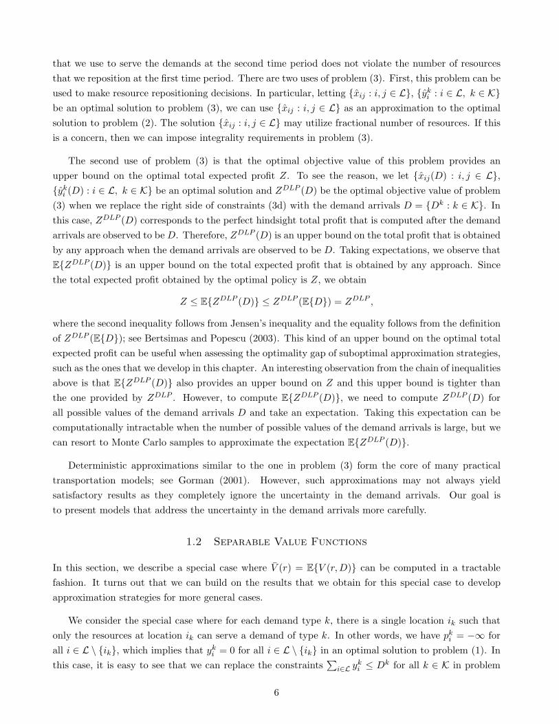
that we use to serve the demands at the second time period does not violate the number of resourcesthat we reposition at the first time period. There are two uses of problem (3). First, this problem can beused to make resource repositioning decisions. In particular, letting {xij : i, j ∈ L}, {yk

i : i ∈ L, k ∈ K}be an optimal solution to problem (3), we can use {xij : i, j ∈ L} as an approximation to the optimalsolution to problem (2). The solution {xij : i, j ∈ L} may utilize fractional number of resources. If thisis a concern, then we can impose integrality requirements in problem (3).

The second use of problem (3) is that the optimal objective value of this problem provides anupper bound on the optimal total expected profit Z. To see the reason, we let {xij(D) : i, j ∈ L},{yk

i (D) : i ∈ L, k ∈ K} be an optimal solution and ZDLP (D) be the optimal objective value of problem(3) when we replace the right side of constraints (3d) with the demand arrivals D = {Dk : k ∈ K}. Inthis case, ZDLP (D) corresponds to the perfect hindsight total profit that is computed after the demandarrivals are observed to be D. Therefore, ZDLP (D) is an upper bound on the total profit that is obtainedby any approach when the demand arrivals are observed to be D. Taking expectations, we observe thatE{ZDLP (D)} is an upper bound on the total expected profit that is obtained by any approach. Sincethe total expected profit obtained by the optimal policy is Z, we obtain

Z ≤ E{ZDLP (D)} ≤ ZDLP (E{D}) = ZDLP ,

where the second inequality follows from Jensen’s inequality and the equality follows from the definitionof ZDLP (E{D}); see Bertsimas and Popescu (2003). This kind of an upper bound on the optimal totalexpected profit can be useful when assessing the optimality gap of suboptimal approximation strategies,such as the ones that we develop in this chapter. An interesting observation from the chain of inequalitiesabove is that E{ZDLP (D)} also provides an upper bound on Z and this upper bound is tighter thanthe one provided by ZDLP . However, to compute E{ZDLP (D)}, we need to compute ZDLP (D) forall possible values of the demand arrivals D and take an expectation. Taking this expectation can becomputationally intractable when the number of possible values of the demand arrivals is large, but wecan resort to Monte Carlo samples to approximate the expectation E{ZDLP (D)}.

Deterministic approximations similar to the one in problem (3) form the core of many practicaltransportation models; see Gorman (2001). However, such approximations may not always yieldsatisfactory results as they completely ignore the uncertainty in the demand arrivals. Our goal isto present models that address the uncertainty in the demand arrivals more carefully.

1.2 Separable Value Functions

In this section, we describe a special case where V (r) = E{V (r,D)} can be computed in a tractablefashion. It turns out that we can build on the results that we obtain for this special case to developapproximation strategies for more general cases.

We consider the special case where for each demand type k, there is a single location ik such thatonly the resources at location ik can serve a demand of type k. In other words, we have pk

i = −∞ forall i ∈ L \ {ik}, which implies that yk

i = 0 for all i ∈ L \ {ik} in an optimal solution to problem (1). Inthis case, it is easy to see that we can replace the constraints

∑i∈L yk

i ≤ Dk for all k ∈ K in problem

6

(1) with the constraints yki ≤ Dk for all i ∈ L, k ∈ K. If we do replace the constraints

∑i∈L yk

i ≤ Dk forall k ∈ K in problem (1) with the constraints yk

i ≤ Dk for all i ∈ L, k ∈ K, then all of the constraintsin problem (1) decompose by the locations, and we can obtain an optimal solution to problem (1) byconcentrating on one location at a time. In particular, the subproblem for location i is of the form

Vi(ri, D) = max∑

k∈Kpk

i yki (4a)

subject to∑

k∈Kyk

i ≤ ri (4b)

yki ≤ Dk ∀ k ∈ K (4c)

yki ∈ Z+ ∀ k ∈ K, (4d)

and we have V (r,D) =∑

i∈L Vi(ri, D). An important observation is that problem (4) is a knapsackproblem. The capacity of the knapsack is ri. There are |K| items, each item occupies one unit of space,and we can put at most Dk units of item k into the knapsack. Therefore, it is possible to solve problem(4) by sorting the objective function coefficients of the items and putting the items into the knapsackstarting from the item with the largest objective function coefficient.

We need the value function V (r) =∑

i∈L E{Vi(ri, D)} to compute the optimal repositioning decisionsthrough problem (2). It turns out that taking this expectation is tractable due to the knapsack structureof problem (4). We assume without loss of generality that the set of demand types is K = {1, 2, . . . , K},and the demand types are ordered such that p1

i ≥ p2i ≥ . . . ≥ pK

i . Noting the knapsack interpretationof problem (4), we let ψk

i (q) be the probability that the kth item uses the qth unit of available spacein the knapsack for location i. In this case, the expected revenue that we generate from the qth unit ofavailable space becomes

∑k∈K ψk

i (q) pki , and the expectation of the optimal objective value of problem

(4) can be computed as

E{Vi(ri, D)} =ri∑

q=1

∑

k∈Kψk

i (q) pki .

To compute ψki (q), we observe that for the kth item to use the qth unit of available space in the

knapsack, the total amount of space used by the first k− 1 items should be strictly smaller than q, thetotal amount of space used by the first k items should be greater than or equal to q, and item k shouldsatisfy ik = i, since otherwise we have pk

i = −∞ and it is never desirable to put the kth item into theknapsack. Therefore, we have ψk

i (q) = P{D1 + . . .+Dk−1 < q ≤ D1 + . . .+Dk} if ik = i, and ψki (q) = 0

otherwise. This implies that we can compute ψki (q) in a tractable fashion as long as we can compute the

convolutions of the distributions of {Dk : k ∈ K}, which is the case when the demand random variableshave, for example, independent Poisson distributions.

The approach outlined above is proposed by Cheung (1994). Powell and Cheung (1994a), Powelland Cheung (1994b), Cheung and Powell (1996a) and Cheung and Powell (1996b) apply this approachto a variety of settings, including dynamic fleet management and inventory distribution. An interestingaspect of this approach is that it not only allows us to compute V (r) = E{V (r,D)} in a special case,but also allows us to construct approximations when the special case does not necessarily hold. This isthe topic of the next section.

7

1.3 Decomposition by Demand Relaxation

In this section, we demonstrate how we can build on the special case that we discuss in Section 1.2 toconstruct tractable approximation strategies for more general cases. The fundamental idea is to relaxconstraints (1c) in problem (1) by associating the nonnegative Lagrange multipliers λ = {λk : k ∈ K}with them. In this case, the relaxed version of problem (1) becomes

V DDR(r,D, λ) = max∑

i∈L

∑

k∈K[pk

i − λk] yki +

∑

k∈Kλk Dk (5a)

subject to∑

k∈Kyk

i ≤ ri ∀ i ∈ L (5b)

yki ≤ Dk ∀ i ∈ L, k ∈ K (5c)

yki ∈ Z+ ∀ i ∈ L, k ∈ K. (5d)

Constraints (5c) would be redundant in problem (1), but we add them to the problem above to tightenthe relaxation. We use the argument λ in the value function V DDR(r,D, λ) to emphasize that theoptimal objective value of problem (5) depends on the Lagrange multipliers that we associate withthe constraints

∑i∈L yk

i ≤ Dk for all k ∈ K. The superscript DDR in the value function stands fordecomposition by demand relaxation.

Noting that all of the constraints in problem (5) decompose by the locations, we can obtain anoptimal solution to this problem by concentrating on one location at a time. In this case, the subproblemfor location i has the same form as problem (4) with the exception that the objective function of thesubproblem for location i now reads

∑k∈K[ pk

i − λk] yki instead of

∑k∈K pk

i yki . This implies that we

can compute E{V DDR(r,D, λ)} in a tractable fashion by using the approach that we describe in theprevious section. Furthermore, it is possible to show that the demand relaxation strategy provides anupper bound on the optimal total expected profit. To see the reason, we let {yk

i : i ∈ L, k ∈ K} be anoptimal solution to problem (1) and note that

V (r,D) =∑

i∈L

∑

k∈Kpk

i yki ≤

∑

i∈L

∑

k∈K[pk

i − λk] yki +

∑

k∈Kλk Dk ≤ V DDR(r,D, λ). (6)

The first inequality follows from the fact the Lagrange multipliers are nonnegative and we have∑i∈L yk

i ≤ Dk for all k ∈ K by constraints (1c) in problem (1). The second inequality follows from thefact that {yk

i : i ∈ L, k ∈ K} is a feasible but not necessarily an optimal solution to problem (5). Takingexpectations, we obtain V (r) = E{V (r,D)} ≤ E{V DDR(r,D, λ)}. Therefore, if we replace V (r) in theobjective function of problem (2) with E{V DDR(r,D, λ)} and solve this problem, then the resultingobjective function value ZDDR(λ) provides an upper bound on the optimal total expected profit Z, aslong as the Lagrange multipliers are nonnegative.

There are several approaches that we can use to choose a good set of Lagrange multipliers. Tobegin with, we note that ZDDR(λ) ≥ Z whenever we have λ ≥ 0. Therefore, we can solve the problemminλ≥0 ZDDR(λ) to obtain the tightest possible upper bound on the optimal total expected profit anduse the optimal solution to this problem as the Lagrange multipliers. Cheung and Powell (1996b) showthat ZDDR(λ) is a convex function of λ so that the problem minλ≥0 ZDDR(λ) can be solved by using

8

standard subgradient optimization. A possible shortcoming of this approach is that solving the problemminλ≥0 ZDDR(λ) can be time consuming. Kunnumkal and Topaloglu (2008b) propose another approachfor choosing the Lagrange multipliers that uses the dual solution to problem (3). In particular, theynote that constraints (3d) in problem (3) are analogous to constraints (1c) in problem (1). In this case,letting λ = {λk : k ∈ K} be the optimal values of the dual variables associated with constraints (3d) inproblem (3), they choose the Lagrange multipliers as λ. Since λ ≥ 0 by dual feasibility to problem (3),we have ZDDR(λ) ≥ Z. Furthermore, Kunnumkal and Topaloglu (2008b) show that ZDDR(λ) ≤ ZDLP ,and we obtain

Z ≤ minλ≥0

ZDDR(λ) ≤ ZDDR(λ) ≤ ZDLP .

Therefore, the demand relaxation strategy provides an upper bound on the optimal total expectedprofit, and this upper bound is tighter than the one provided by the deterministic approximation.

The demand relaxation strategy is proposed by Cheung (1994), but the idea of relaxing complicatingconstraints in stochastic optimization problems frequently appears in the literature. Ruszczynski (2003)gives an overview of this idea within the framework of general stochastic programs. Adelman andMersereau (2008) introduce the term “weakly coupled dynamic program” to refer to a stochasticoptimization problem which would decompose if a few linking constraints did not exist. They study adual framework for such stochastic optimization problems. Cheung and Powell (1996a) and Cheung andPowell (1996b) provide applications of the demand relaxation strategy to dynamic fleet managementand inventory distribution problems. Similar relaxation ideas are used by Castanon (1997), Yost andWashburn (2000) and Bertsimas and Mersereau (2007) in partially observable Markov decision processes,by Federgruen and Zipkin (1984), Topaloglu and Kunnumkal (2006) and Kunnumkal and Topaloglu(2008a) in inventory distribution and by Erdelyi and Topaloglu (2009b), Kunnumkal and Topaloglu(2009b) and Topaloglu (2009b) in airline network revenue management.

1.4 Decomposition by Supply Relaxation

In this section, we construct a tractable approximation strategy by using a relaxation idea that isconceptually similar to the one in the previous section, but the specific details of this relaxation ideaare quite different. We begin by choosing an arbitrary location i and relax constraints (1b) in problem(1) for all other locations by associating the nonnegative Lagrange multipliers µ = {µj : j ∈ L \ {i}}with them. In this case, the relaxed version of problem (1) becomes

V DSRi (r,D, µ) = max

∑

k∈Kpk

i yki +

∑

j∈L\{i}

∑

k∈K[pk

j − µj ] ykj +

∑

j∈L\{i}µj rj (7a)

subject to∑

k∈Kyk

i ≤ ri (7b)

yki +

∑

j∈L\{i}yk

j ≤ Dk ∀ k ∈ K (7c)

yki , yk

j ∈ Z+ ∀ j ∈ L \ {i}, k ∈ K. (7d)

9

The subscript i in the value function V DSRi (r,D, µ) emphasizes that the optimal objective value of the

problem above depends on the choice of location i, and the superscript DSR stands for decompositionby supply relaxation.

It is possible to show that problem (7) has the same structure as problem (4), in which case, we cancompute E{V DSR

i (r,D, µ)} by using the approach that we describe in Section 1.2. To see the equivalencebetween problems (4) and (7), we first observe that the decision variables {yk

j : j ∈ L \ {i}, k ∈ K}appear only in constraints (7c) in problem (7). This implies that we can replace the decision variables{yk

j : j ∈ L \ {i}} with a single decision variable, and the objective function coefficient of this decisionvariable would be maxj∈L\{i}[pk

j−µj ]. Therefore, letting ρk = maxj∈L\{i}[pkj−µj ] for notational brevity

and replacing the decision variables {ykj : j ∈ L \ {i}} with the single decision variable zk, problem (7)

can be written as

max∑

k∈Kpk

i yki +

∑

k∈Kρk zk +

∑

j∈L\{i}µj rj (8a)

subject to∑

k∈Kyk

i ≤ ri (8b)

yki + zk ≤ Dk ∀ k ∈ K (8c)

yki , zk ∈ Z+ ∀ k ∈ K. (8d)

We assume without loss of generality that ρk ≥ 0 for all k ∈ K. If there exists some k ∈ K such thatρk < 0, then the corresponding decision variable zk takes value zero in an optimal solution, and thisdecision variable can be dropped from problem (8) without changing the optimal objective value. Sincewe have ρk ≥ 0 for all k ∈ K, the decision variables {zk : k ∈ K} take their largest possible values inan optimal solution, and the largest possible values of these decision variables are {Dk − yk

i : k ∈ K}.Therefore, we can replace the decision variables {zk : k ∈ K} in the problem above with {Dk−yk

i : k ∈ K}and obtain the equivalent problem

max∑

k∈K[pk

i − ρk] yki +

∑

k∈Kρk Dk +

∑

j∈L\{i}µj rj (9a)

subject to∑

k∈Kyk

i ≤ ri (9b)

yki ≤ Dk ∀ k ∈ K (9c)

yki ∈ Z+ ∀ k ∈ K. (9d)

Ignoring the constant terms∑

k∈K ρk Dk and∑

j∈L\{i} µj rj , problem (9) has the same structure asproblem (4). By using an argument similar to the one in (6), we can show that V (r,D) ≤ V DSR

i (r,D, µ)as long as the Lagrange multipliers are nonnegative; see Zhang and Adelman (2009).

Since the choice of location i is arbitrary, we have V (r,D) ≤ V DSRi (r,D, µ) for all i ∈ L, and it is not

clear which one of {V DSRi (r,D, µ) : i ∈ L} we should use as an approximation to V (r,D). We resolve

this ambiguity by averaging over all i ∈ L and using 1|L|

∑i∈L V DSR

i (r,D, µ) as an approximation toV (r,D). Noting that V DSR

i (r,D, µ) is an upper bound on V (r,D) for all i ∈ L, 1|L|

∑i∈L V DSR

i (r,D, µ)is also an upper bound on V (r,D). In this case, if we replace V (r) in the objective function of problem

10

(2) with 1|L|

∑i∈L E{V DSR

i (r,D, µ)} and solve this problem, then the resulting objective function valueZDSR(µ) provides an upper bound on the optimal total expected profit Z, as long as we have µ ≥ 0.

The methods that we use to choose a good set of Lagrange multipliers are similar to those in Section1.3. In particular, we can solve the problem minµ≥0 ZDSR(µ) to obtain the tightest possible upperbound on Z and use the optimal solution to this problem as the Lagrange multipliers. It is possible toshow that ZDSR(µ) is a convex function of µ so that we can solve the problem minµ≥0 ZDSR(µ) by usingstandard subgradient optimization. Another approach for choosing a good set of Lagrange multipliersis based on the dual solution of problem (3). We note that constraints (1b) in problem (1) capturethe resource availabilities at different locations at the beginning of the second time period. Similarly,constraints (3c) in problem (3) capture the resource availabilities at different locations. Therefore,letting {µi : i ∈ L} be the optimal values of the dual variables associated with constraints (3c) inproblem (3), we can choose the Lagrange multipliers as {µj : j ∈ L \ {i}}.

The supply relaxation strategy has its roots in the network revenue management literature. In thisliterature, it is customary to relax the capacity constraints for all of the flight legs except for one and toobtain approximations to the value function by concentrating on one flight leg at a time; see Talluri andvan Ryzin (2005). Zhang and Adelman (2009) establish that the supply relaxation strategy provides anupper bound on the value function. Kunnumkal and Topaloglu (2008c) and Kunnumkal and Topaloglu(2009a) provide alternative proofs for the same result. Erdelyi and Topaloglu (2009a) use the supplyrelaxation idea to solve an overbooking problem. Topaloglu (2009a) extends the supply relaxationstrategy to general stochastic programs and provides applications in dynamic fleet management.

1.5 Separable Projective Approximations

In this section, we describe an iterative approach that uses sampled realizations of the demand arrivalsto construct a separable approximation to the value function. The fundamental idea is to approximatethe value function V (r) with a separable function of the form

V SPA(r) =∑

i∈LV SPA

i (ri),

where the approximations {V SPAi (·) : i ∈ L} are single dimensional, piecewise linear and concave

functions with points of nondifferentiability being a subset of integers. The superscript SPA standsfor separable projective approximations. The concavity of the approximation V SPA

i (·) is intended tocapture the intuitive expectation that the marginal benefit from an additional resource at a locationshould be decreasing as we have more resources available at the location. Noting that V SPA

i (·) is apiecewise linear function with points of nondifferentiability being a subset of integers, if we have a totalof Q available resources, then we can characterize the approximation V SPA

i (·) with a sequence of Q

slopes {vi(q) : q = 0, . . . , Q− 1}, where vi(q) is the slope of V SPAi (·) over the interval [q, q +1]. In other

words, we have vi(q) = V SPAi (q + 1)− V SPA

i (q).

We use an iterative approach to construct the approximations {V SPAi (·) : i ∈ L}. In particular,

letting {V SPA,ni (·) : i ∈ L} be the approximations at iteration n, we begin by solving problem (2)

11

Step 1. Initialize the iteration counter by letting n = 1. Initialize the approximations {V SPA,1i (·) : i ∈ L}

to arbitrary piecewise linear and concave functions with points of nondifferentiability being asubset of integers.

Step 2. Solve problem (2) after replacing V (r) in the objective function with the value functionapproximation

∑i∈L V SPA,n

i (ri). Let {xnij : i, j ∈ L}, {rn

i : i ∈ L} be an optimal solution.

Step 3. Sample a realization of the demand arrivals and denote this sample by {Dk,n : k ∈ K}. Solveproblem (1) after replacing the right side of constraints (1b) with rn = {rn

i : i ∈ L} and the rightside of constraints (1c) with Dn = {Dk,n : k ∈ K}.

Step 4. Use the solution to problem (1) to update the approximations {V SPA,ni (·) : i ∈ L} and obtain the

approximations {V SPA,n+1i (·) : i ∈ L} that is used at the next iteration. Increase n by one and

go to Step 2.

Figure 1: An iterative approach to construct a separable value function approximation.

after replacing V (r) in the objective function with∑

i∈L V SPA,ni (ri). This provides an optimal solution

{xnij : i, j ∈ L}, {rn

i : i ∈ L}. We then sample a realization of the demand arrivals, which we denoteby {Dk,n : k ∈ K}. We solve problem (1) after replacing the right side of constraints (1b) withrn = {rn

i : i ∈ L} and the right side of constraints (1c) with Dn = {Dk,n : k ∈ K}. The challenge is touse the solution to problem (1) to improve the approximations {V SPA,n

i (·) : i ∈ L}. We give a descriptionof the general approach in Figure 1. In Step 1, we initialize the approximations {V SPA,n

i (·) : i ∈ L}to arbitrary piecewise linear and concave functions with points of nondifferentiability being a subset ofintegers. In Step 2, we solve problem (2) after replacing V (r) in the objective function with the valuefunction approximation

∑i∈L V SPA,n

i (ri). In Step 3, we sample a realization of the demand arrivalsand solve problem (1) by using the sampled demand arrivals and the resource availabilities obtainedfrom problem (2). In Step 4, we update the approximations {V SPA,n

i (·) : i ∈ L}, and this provides theapproximations {V SPA,n+1

i (·) : i ∈ L} that we use at the next iteration.

The approach that we use to update the approximations is based on a stochastic approximationidea, but we need to be careful to preserve the concavity of the value function approximation. Usingei to denote the |L| dimensional unit vector with a one in the element corresponding to i ∈ L, welet ϑn

i = V (rn + ei, Dn) − V (rn, Dn). Therefore, ϑn

i captures the marginal benefit from an additionalresource at location i in problem (1) when the number of resources at different locations is given byrn = {rn

i : i ∈ L} and the realization of the demand arrivals is given by Dn = {Dk,n : k ∈ K}. In thiscase, letting V SPA,n

i (·) be the piecewise linear and concave function characterized by the sequence ofslopes {vn

i (q) : q = 0, . . . , Q− 1}, we update these slopes as

γni (q) =

{[1− αn] vn

i (q) + αn ϑni if q = rn

i

vni (q) otherwise,

12

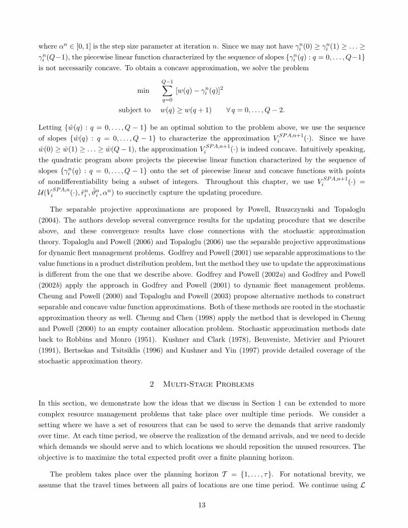
where αn ∈ [0, 1] is the step size parameter at iteration n. Since we may not have γni (0) ≥ γn

i (1) ≥ . . . ≥γn

i (Q−1), the piecewise linear function characterized by the sequence of slopes {γni (q) : q = 0, . . . , Q−1}

is not necessarily concave. To obtain a concave approximation, we solve the problem

minQ−1∑

q=0

[w(q)− γni (q)]2

subject to w(q) ≥ w(q + 1) ∀ q = 0, . . . , Q− 2.

Letting {w(q) : q = 0, . . . , Q − 1} be an optimal solution to the problem above, we use the sequenceof slopes {w(q) : q = 0, . . . , Q − 1} to characterize the approximation V SPA,n+1

i (·). Since we havew(0) ≥ w(1) ≥ . . . ≥ w(Q− 1), the approximation V SPA,n+1

i (·) is indeed concave. Intuitively speaking,the quadratic program above projects the piecewise linear function characterized by the sequence ofslopes {γn

i (q) : q = 0, . . . , Q − 1} onto the set of piecewise linear and concave functions with pointsof nondifferentiability being a subset of integers. Throughout this chapter, we use V SPA,n+1

i (·) =U(V SPA,n

i (·), rni , ϑn

i , αn) to succinctly capture the updating procedure.

The separable projective approximations are proposed by Powell, Ruszczynski and Topaloglu(2004). The authors develop several convergence results for the updating procedure that we describeabove, and these convergence results have close connections with the stochastic approximationtheory. Topaloglu and Powell (2006) and Topaloglu (2006) use the separable projective approximationsfor dynamic fleet management problems. Godfrey and Powell (2001) use separable approximations to thevalue functions in a product distribution problem, but the method they use to update the approximationsis different from the one that we describe above. Godfrey and Powell (2002a) and Godfrey and Powell(2002b) apply the approach in Godfrey and Powell (2001) to dynamic fleet management problems.Cheung and Powell (2000) and Topaloglu and Powell (2003) propose alternative methods to constructseparable and concave value function approximations. Both of these methods are rooted in the stochasticapproximation theory as well. Cheung and Chen (1998) apply the method that is developed in Cheungand Powell (2000) to an empty container allocation problem. Stochastic approximation methods dateback to Robbins and Monro (1951). Kushner and Clark (1978), Benveniste, Metivier and Priouret(1991), Bertsekas and Tsitsiklis (1996) and Kushner and Yin (1997) provide detailed coverage of thestochastic approximation theory.

2 Multi-Stage Problems

In this section, we demonstrate how the ideas that we discuss in Section 1 can be extended to morecomplex resource management problems that take place over multiple time periods. We consider asetting where we have a set of resources that can be used to serve the demands that arrive randomlyover time. At each time period, we observe the realization of the demand arrivals, and we need to decidewhich demands we should serve and to which locations we should reposition the unused resources. Theobjective is to maximize the total expected profit over a finite planning horizon.

The problem takes place over the planning horizon T = {1, . . . , τ}. For notational brevity, weassume that the travel times between all pairs of locations are one time period. We continue using L

13

to denote the set of locations in the transportation network. To capture the decisions, we let xijt bethe number of resources that we reposition from location i to j at time period t and yk

it be the numberof demands of type k that we serve by using a resource at location i at time period t. The cost ofrepositioning one resource from location i to j is cij . If we serve a demand of type k by using a resourceat location i, then we generate a revenue of pk

i , and the resource ends up at location δk at the next timeperiod. Similar to the convention that we use in Section 1, if it is infeasible to serve a demand of typek by using a resource at location i, then we assume that pk

i = −∞. We use the random variable Dkt to

represent the number of demands of type k that arrive at time period t. We assume that the demandarrivals at different time periods are independent. We let rit be the number of resources available atlocation i at the beginning of time period t. We note that {ri1 : i ∈ L} is a part of the problem data,whereas {rit : i ∈ L} for t ∈ T \ {1} is determined by the decisions at time period t− 1.

We can formulate the problem as a dynamic program by using rt = {rit : i ∈ L} as the statevariable at time period t. Letting 1(·) be the indicator function, and using xt = {xijt : i, j ∈ L} andyt = {yk

it : i ∈ L, k ∈ K} to capture the decisions and Dt = {Dkt : k ∈ K} to capture the demand

arrivals at time period t, the set of feasible decisions and state transitions are given by

X (rt, Dt) ={

(xt, yt, rt+1) :∑

j∈Lxijt +

∑

k∈Kyk

it = rit ∀ i ∈ L (10a)

∑

i∈Lxijt +

∑

i∈L

∑

k∈K1(δk = j) yk

it − rj,t+1 = 0 ∀ j ∈ L (10b)

∑

i∈Lyk

it ≤ Dkt ∀ k ∈ K (10c)

xijt, ykit, rj,t+1 ∈ Z+ ∀ i, j ∈ L, k ∈ K

}. (10d)

Constraints (10a) ensure that the number of resources that we reposition between different locationsand use to serve the demands does not violate the resource availabilities. Constraints (10b) compute thenumber of resources available at different locations at the beginning of the next time period. Constraints(10c) ensure that the number of demands that we serve does not exceed the demand arrivals. We canfind the optimal policy by computing the value functions {Vt(·) : t ∈ T } through the optimality equation

Vt(rt) = E

{max

(xt,yt,rt+1)∈X (rt,Dt)−

∑

i∈L

∑

j∈Lcij xijt +

∑

i∈L

∑

k∈Kpk

i ykit + Vt+1(rt+1)

}

with the boundary condition that Vτ+1(·) = 0; see Puterman (1994). The optimality equation aboveinvolves a high dimensional state variable, which makes it difficult to compute the value functions forall possible values of the vector rt. This difficulty is further compounded by the fact that the decisions(xt, yt) in the problem above are high dimensional vectors, and we take an expectation that involvesthe high dimensional demand arrivals Dt. Powell (2007) uses the term “three curses of dimensionality”to refer to the difficulty due to the sizes of the state, decision and demand vectors.

It turns out that all of the ideas in Section 1 can be extended to multi-stage problems. For economyof space, we only show extensions of the deterministic linear program and the separable projectiveapproximations. Cheung and Powell (1996b) extend the demand relaxation strategy and Topaloglu(2009a) extends the supply relaxation strategy to multi-stage problems.

14

2.1 Deterministic Linear Program

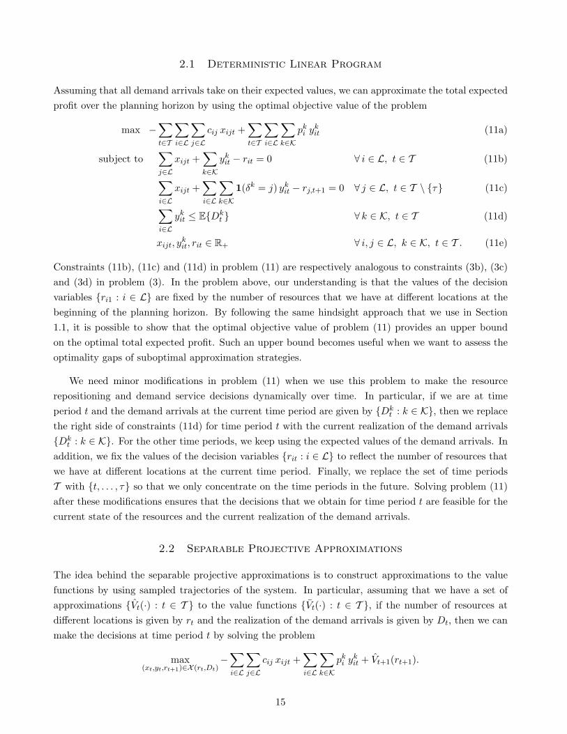
Assuming that all demand arrivals take on their expected values, we can approximate the total expectedprofit over the planning horizon by using the optimal objective value of the problem

max −∑

t∈T

∑

i∈L

∑

j∈Lcij xijt +

∑

t∈T

∑

i∈L

∑

k∈Kpk

i ykit (11a)

subject to∑

j∈Lxijt +

∑

k∈Kyk

it − rit = 0 ∀ i ∈ L, t ∈ T (11b)

∑

i∈Lxijt +

∑

i∈L

∑

k∈K1(δk = j) yk

it − rj,t+1 = 0 ∀ j ∈ L, t ∈ T \ {τ} (11c)

∑

i∈Lyk

it ≤ E{Dkt } ∀ k ∈ K, t ∈ T (11d)

xijt, ykit, rit ∈ R+ ∀ i, j ∈ L, k ∈ K, t ∈ T . (11e)

Constraints (11b), (11c) and (11d) in problem (11) are respectively analogous to constraints (3b), (3c)and (3d) in problem (3). In the problem above, our understanding is that the values of the decisionvariables {ri1 : i ∈ L} are fixed by the number of resources that we have at different locations at thebeginning of the planning horizon. By following the same hindsight approach that we use in Section1.1, it is possible to show that the optimal objective value of problem (11) provides an upper boundon the optimal total expected profit. Such an upper bound becomes useful when we want to assess theoptimality gaps of suboptimal approximation strategies.

We need minor modifications in problem (11) when we use this problem to make the resourcerepositioning and demand service decisions dynamically over time. In particular, if we are at timeperiod t and the demand arrivals at the current time period are given by {Dk

t : k ∈ K}, then we replacethe right side of constraints (11d) for time period t with the current realization of the demand arrivals{Dk

t : k ∈ K}. For the other time periods, we keep using the expected values of the demand arrivals. Inaddition, we fix the values of the decision variables {rit : i ∈ L} to reflect the number of resources thatwe have at different locations at the current time period. Finally, we replace the set of time periodsT with {t, . . . , τ} so that we only concentrate on the time periods in the future. Solving problem (11)after these modifications ensures that the decisions that we obtain for time period t are feasible for thecurrent state of the resources and the current realization of the demand arrivals.

2.2 Separable Projective Approximations

The idea behind the separable projective approximations is to construct approximations to the valuefunctions by using sampled trajectories of the system. In particular, assuming that we have a set ofapproximations {Vt(·) : t ∈ T } to the value functions {Vt(·) : t ∈ T }, if the number of resources atdifferent locations is given by rt and the realization of the demand arrivals is given by Dt, then we canmake the decisions at time period t by solving the problem

max(xt,yt,rt+1)∈X (rt,Dt)

−∑

i∈L

∑

j∈Lcij xijt +

∑

i∈L

∑

k∈Kpk

i ykit + Vt+1(rt+1).

15

Therefore, repeated solutions of the problem above for the successive time periods in the planninghorizon would allow us to simulate the trajectory of the system under a particular realization of thedemand arrivals. The challenge is to use the information that we obtain from the simulated trajectoriesof the system to update and improve the value function approximations.

We use the separable functions {V SPAt (·) : t ∈ T } as our value function approximations. Similar

to the development in Section 1.5, each one of these value function approximations is of the formV SPA

t (rt) =∑

i∈L V SPAit (rit), where V SPA

it (·) is a single dimensional, piecewise linear and concavefunction with points of nondifferentiability being a subset of integers. Letting Q be the total number ofavailable resources, we can characterize V SPA

it (·) by the sequence of slopes {vit(q) : q = 0, . . . , Q − 1},where vit(q) is the slope of V SPA

it (·) over the interval [q, q + 1].

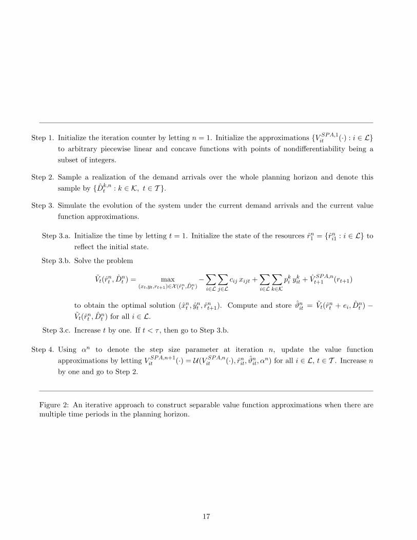
The updating procedure in Section 1.5, together with the idea of simulating the trajectories ofthe system, immediately provides an iterative method that can be used to construct separable valuefunction approximations. We describe this method in Figure 2. In Step 1, we initialize the valuefunction approximations. In Step 2, we sample a realization of the demand arrivals over the wholeplanning horizon. In Step 3, we simulate the evolution of the system under the current demand arrivalsand the current value function approximations. In Step 4, we update the value function approximationsto obtain the value function approximations that we use at the next iteration. The updating procedureU(V SPA,n

it (·), rnit, ϑ

nit, α

n) in this step is identical to the one that we describe in Section 1.5.

3 A Flexible Modeling Framework

The resource management problems that we have considered thus far are relatively simplistic. Inparticular, the only distinguishing characteristic of a resource is its location, whereas the onlydistinguishing characteristic of a demand is its type. Our motivation for working with somewhatsimplistic resource management problems is that such problems allow us to demonstrate the crucialalgorithmic issues more clearly, but practical resource management problems can easily take on muchmore complex characteristics. For example, a driver resource in a driver scheduling application can bedescribed by its inbound location, time to reach the inbound location, duty time within the shift, daysaway from home, vehicle type and home domicile. Conceptually, we can model such a complex resourceby using multiple indices in our decision and state variables to capture the different attributes of theresource, but this approach would clearly be too cumbersome. In this section, we describe a flexibleparadigm that is useful for modeling complex resource management problems.

3.1 Resources

To represent the resources, we let A be the attribute space of the resources. Roughly speaking, theattribute space represents the set of all possible states of a particular resource. We refer to each elementof the attribute space as an attribute vector. We let rat be the number of resources with attribute vectora at time period t. For example, if we assume that the set of locations is L, the set of vehicle typesis V and the travel time between any pair of locations is bounded by T , then the attribute space for

16

Step 1. Initialize the iteration counter by letting n = 1. Initialize the approximations {V SPA,1it (·) : i ∈ L}

to arbitrary piecewise linear and concave functions with points of nondifferentiability being asubset of integers.

Step 2. Sample a realization of the demand arrivals over the whole planning horizon and denote thissample by {Dk,n

t : k ∈ K, t ∈ T }.

Step 3. Simulate the evolution of the system under the current demand arrivals and the current valuefunction approximations.

Step 3.a. Initialize the time by letting t = 1. Initialize the state of the resources rn1 = {rn

i1 : i ∈ L} toreflect the initial state.

Step 3.b. Solve the problem

Vt(rnt , Dn

t ) = max(xt,yt,rt+1)∈X (rn

t ,Dnt )−

∑

i∈L

∑

j∈Lcij xijt +

∑

i∈L

∑

k∈Kpk

i ykit + V SPA,n

t+1 (rt+1)

to obtain the optimal solution (xnt , yn

t , rnt+1). Compute and store ϑn

it = Vt(rnt + ei, D

nt ) −

Vt(rnt , Dn

t ) for all i ∈ L.

Step 3.c. Increase t by one. If t < τ , then go to Step 3.b.

Step 4. Using αn to denote the step size parameter at iteration n, update the value functionapproximations by letting V SPA,n+1

it (·) = U(V SPA,nit (·), rn

it, ϑnit, α

n) for all i ∈ L, t ∈ T . Increase n

by one and go to Step 2.

Figure 2: An iterative approach to construct separable value function approximations when there aremultiple time periods in the planning horizon.

17

the vehicles in a simple dynamic fleet management application is A = L × V × {0, 1, . . . , T}. A vehiclewith the attribute vector a = (a1, a2, a3) = (New York, Large, 4) ∈ A is a vehicle of type large thatis inbound to New York and will reach New York in four time periods. We can access the number ofresources with attribute vector a at time period t by referring to rat. This implies that we can lumpthe resources with the same attribute vector together and treat them as indistinguishable.

We use a similar approach to represent the demands. We let B be the attribute space of the demandsand Dbt be the number of demands with attribute vector b at time period t. For example, if the set ofexpedition options is E , then the attribute space for the demands may be B = L × L × E . A demandwith the attribute vector b = (b1, b2, b3) = (New York, Delaware, Express) ∈ B is an express demandwith origin location New York and destination location Delaware. It may be not possible to serve anexpress demand from New York to Delaware by using a vehicle in New Jersey, but if the demand is notexpress, then it may be the case that a vehicle in New Jersey can serve this demand. Therefore, thecharacteristics of the demand may dictate the feasible resource assignments.

3.2 Decisions

We use two classes of decisions. The class of decisions DR captures the repositioning decisions, whereasthe class of decisions DS captures the demand service decisions. We let D = DR ∪ DS to capture theset of all decision classes and refer to each element of D as a decision. For example, we may haveDR = L × L, and the decision d = (d1, d2) = (New York, Delaware) ∈ DR may represent the decisionto reposition a resource from New York to Delaware. Similarly, we may have DS = B, and the decisiond = (b1, b2, b3) ∈ DS = B may represent the decision to serve a demand with the attribute vector b. Itis reasonable to assume that for each decision d ∈ DS , there exists an attribute vector bd ∈ B such thatthe decision d corresponds to serving a demand with attribute vector bd.

We use xadt to denote the number of resources with attribute vector a that we modify by usingdecision d at time period t. If we modify a resource with attribute vector a by using decision d at timeperiod t, then we generate a profit contribution of cadt. If it is not feasible to apply decision d on aresource with attribute vector a, then we capture this situation by letting cadt = −∞. In this case, wecan capture the decisions at time period t by xt = {xadt : a ∈ A, d ∈ D}, the state of the resources byrt = {rat : a ∈ A} and the state of the demands by Dt = {Dbt : b ∈ B}.

3.3 Optimization Problem

The set of feasible decisions at time period t is given by

X (rt, Dt) ={

xt :∑

d∈Dxadt = rat ∀ a ∈ A (12a)

∑

a∈Axadt ≤ Dbd,t ∀ d ∈ DS (12b)

xadt ∈ Z+ ∀ a ∈ A, d ∈ D}

, (12c)

18

where we use the fact that for each decision d ∈ DS , there exists an attribute vector bd ∈ B such thatthe decision d corresponds to serving a demand with attribute vector bd. We note that constraints(12a) and (12b) are respectively analogous to constraints (10a) and (10c). We capture the outcome ofapplying a decision d on a resource with attribute vector a by defining

δa′(a, d)

1 if applying the decision d on a resource with attribute vector a transforms the resourceinto a resource with attribute vector a′

0 otherwise.

The precise definition of δa′(a, d) is naturally dependent on the physics of the problem and how thesystem reacts to decisions. Using the definition above, we can write the dynamics of the resources as

ra,t+1 =∑

a′∈A

∑

d∈Dδa(a′, d) xa′dt ∀ a ∈ A,

which are analogous to constraints (10b). The implicit assumption in the definition of δa′(a, d) is that thecurrent attribute vector of the resource and the decision that we apply on the resource deterministicallygive the future attribute vector of the resource. This is indeed the case in many resource managementapplications, but there may be settings with random travel times and equipment failures where thisassumption is not necessarily satisfied.

A Markovian policy π is a collection of decision functions {Xπt (·) : t ∈ T } such that each Xπ

t (·)maps the state of the system (rt, Dt) to a decision vector xt ∈ X (rt, Dt). Our goal is to find a policythat maximizes the total expected profit over the planning horizon. In other words, using Ct(xt) =∑

a∈A∑

d∈D cadt xadt to denote the total profit associated with the decisions xt at time period t and Πto denote the set of all Markovian policies, we want to solve the problem

supπ∈Π

E

{ ∑

t∈TCt(Xπ

t (rt, Dt))

}.

The formulation above provides a compact representation of the resource management problem that weare interested in, but it does not help from an algorithmic perspective. In particular, it is impossibleto make a direct search over a reasonably broad class of policies Π. Therefore, the modeling frameworkthat we describe in this section is useful for communicating the problem, but the actual solution requiresa concrete algorithmic approach such as the ones described in Sections 1 and 2.

The modeling framework that we describe in this section is due to Shapiro (1999) and Powell, Shapiroand Simao (2001). These works are intended to capture a broad class of resource management problemsarising from a variety of application settings, and their presentation is significantly larger in scope thanours. Powell (2007) uses this modeling framework to come up with a sound formulation for generaldynamic programs, with a particular emphasis on the evolution of information over time. Shapiro andPowell (2006) demonstrate how to use the modeling framework within the context of several algorithmicapproaches to decompose large scale resource management problems. Powell, Shapiro and Simao (2002),Powell and Topaloglu (2003), Powell, Wu, Simao and Whisman (2004), Powell and Topaloglu (2005),Schenk and Klabjan (2008) and Simao, Day, George, Gifford, Nienow and Powell (2009) apply the

19

modeling framework to dynamic fleet management, military airlift operations, express package routingand driver scheduling problems. We note that the presentation in this chapter uses demands as the onlysource of uncertainty. The driver scheduling application in Simao et al. (2009) is particularly interestingas it models a variety of sources of uncertainty, such as random travel times, equipment failures anddriver availability.

4 Numerical Illustrations

In this section, we numerically compare the performances of the different approximation strategies thatwe describe in Sections 1 and 2. Our goal here is to give a feel for the relative performances of thedifferent approximation strategies, rather than to present a full scale experimental study.

4.1 Numerical Results for Two-Stage Problems

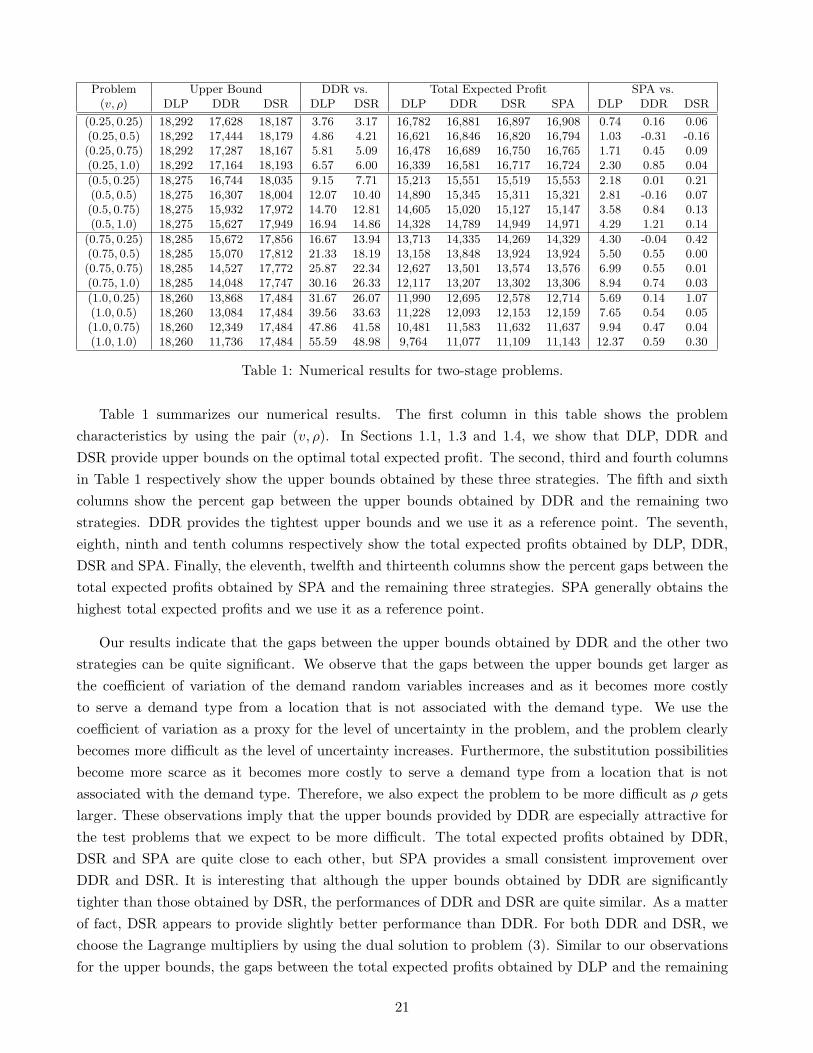
In this section, we provide numerical results for two-stage problems. The test problems that we usein our experimental setup have the same structure as the problem that we describe in Section 1. Wegenerate ten locations uniformly over a 100× 100 region. Using d(i, j) to denote the Euclidean distancebetween locations i and j, the cost of repositioning a resource from location i to j is given by d(i, j). Wehave ten demand types and each demand type is associated with a particular location. The revenuefrom using a resource at location i to serve a demand type that is associated with location j is given by200−ρ×d(i, j), where ρ is a parameter that we vary. As ρ gets larger, it becomes less profitable to servea demand type that is associated with a particular location by using a resource at another location. Inour computational experiments, we vary the coefficient of variation of the demand random variables andthe parameter ρ. In particular, letting v be the coefficient of variation of the demand random variables,we label our test problems by the pair (v, ρ) ∈ {0.25, 0.5, 0.75, 1.0}× {0.25, 0.5, 0.75, 1.0}. We note thatthe numerical results that we present in this section do not appear in the previous literature.

We test the performances of the approximation strategies described in Sections 1.1, 1.3, 1.4 and1.5, which we respectively refer to as DLP, DDR, DSR and SPA. DLP immediately provides a set offirst stage decisions {xij : i, j ∈ L}. On the other hand, DDR, DSR and SPA provide value functionapproximations that are all separable functions of the form

∑i∈L Vi(·). To obtain a set of first stage

decisions {xij : i, j ∈ L}, DDR, DSR and SPA replace V (r) in the objective function of problem (2)with

∑i∈L Vi(ri) and solve this problem. For DDR, DSR and SPA, it is possible to show that each one

of {Vi(·) : i ∈ L} is a piecewise linear and concave function with points of nondifferentiability being asubset of integers. In this case, we can formulate problem (2) with the value function approximation∑

i∈L Vi(·) as a minimum cost network flow problem; see Nemhauser and Wolsey (1988). A set of firststage decisions allow us to compute the cost that we incur at the first stage. In addition, we can computethe number of resources at different locations at the beginning of the second stage by rj =

∑i∈L xij for

all j ∈ L. To check the quality of the first stage decisions, we replace the right side of constraints (1b)in problem (1) with {ri : i ∈ L} and solve this problem for many realizations of demand arrivals. In thisway, we approximate the total expected revenue in the second stage. The total expected profit is thedifference between the total cost and the total expected revenue in the two stages.

20

Problem Upper Bound DDR vs. Total Expected Profit SPA vs.(v, ρ) DLP DDR DSR DLP DSR DLP DDR DSR SPA DLP DDR DSR

(0.25, 0.25) 18,292 17,628 18,187 3.76 3.17 16,782 16,881 16,897 16,908 0.74 0.16 0.06(0.25, 0.5) 18,292 17,444 18,179 4.86 4.21 16,621 16,846 16,820 16,794 1.03 -0.31 -0.16(0.25, 0.75) 18,292 17,287 18,167 5.81 5.09 16,478 16,689 16,750 16,765 1.71 0.45 0.09(0.25, 1.0) 18,292 17,164 18,193 6.57 6.00 16,339 16,581 16,717 16,724 2.30 0.85 0.04

(0.5, 0.25) 18,275 16,744 18,035 9.15 7.71 15,213 15,551 15,519 15,553 2.18 0.01 0.21(0.5, 0.5) 18,275 16,307 18,004 12.07 10.40 14,890 15,345 15,311 15,321 2.81 -0.16 0.07(0.5, 0.75) 18,275 15,932 17,972 14.70 12.81 14,605 15,020 15,127 15,147 3.58 0.84 0.13(0.5, 1.0) 18,275 15,627 17,949 16.94 14.86 14,328 14,789 14,949 14,971 4.29 1.21 0.14

(0.75, 0.25) 18,285 15,672 17,856 16.67 13.94 13,713 14,335 14,269 14,329 4.30 -0.04 0.42(0.75, 0.5) 18,285 15,070 17,812 21.33 18.19 13,158 13,848 13,924 13,924 5.50 0.55 0.00(0.75, 0.75) 18,285 14,527 17,772 25.87 22.34 12,627 13,501 13,574 13,576 6.99 0.55 0.01(0.75, 1.0) 18,285 14,048 17,747 30.16 26.33 12,117 13,207 13,302 13,306 8.94 0.74 0.03

(1.0, 0.25) 18,260 13,868 17,484 31.67 26.07 11,990 12,695 12,578 12,714 5.69 0.14 1.07(1.0, 0.5) 18,260 13,084 17,484 39.56 33.63 11,228 12,093 12,153 12,159 7.65 0.54 0.05(1.0, 0.75) 18,260 12,349 17,484 47.86 41.58 10,481 11,583 11,632 11,637 9.94 0.47 0.04(1.0, 1.0) 18,260 11,736 17,484 55.59 48.98 9,764 11,077 11,109 11,143 12.37 0.59 0.30

Table 1: Numerical results for two-stage problems.

Table 1 summarizes our numerical results. The first column in this table shows the problemcharacteristics by using the pair (v, ρ). In Sections 1.1, 1.3 and 1.4, we show that DLP, DDR andDSR provide upper bounds on the optimal total expected profit. The second, third and fourth columnsin Table 1 respectively show the upper bounds obtained by these three strategies. The fifth and sixthcolumns show the percent gap between the upper bounds obtained by DDR and the remaining twostrategies. DDR provides the tightest upper bounds and we use it as a reference point. The seventh,eighth, ninth and tenth columns respectively show the total expected profits obtained by DLP, DDR,DSR and SPA. Finally, the eleventh, twelfth and thirteenth columns show the percent gaps between thetotal expected profits obtained by SPA and the remaining three strategies. SPA generally obtains thehighest total expected profits and we use it as a reference point.

Our results indicate that the gaps between the upper bounds obtained by DDR and the other twostrategies can be quite significant. We observe that the gaps between the upper bounds get larger asthe coefficient of variation of the demand random variables increases and as it becomes more costlyto serve a demand type from a location that is not associated with the demand type. We use thecoefficient of variation as a proxy for the level of uncertainty in the problem, and the problem clearlybecomes more difficult as the level of uncertainty increases. Furthermore, the substitution possibilitiesbecome more scarce as it becomes more costly to serve a demand type from a location that is notassociated with the demand type. Therefore, we also expect the problem to be more difficult as ρ getslarger. These observations imply that the upper bounds provided by DDR are especially attractive forthe test problems that we expect to be more difficult. The total expected profits obtained by DDR,DSR and SPA are quite close to each other, but SPA provides a small consistent improvement overDDR and DSR. It is interesting that although the upper bounds obtained by DDR are significantlytighter than those obtained by DSR, the performances of DDR and DSR are quite similar. As a matterof fact, DSR appears to provide slightly better performance than DDR. For both DDR and DSR, wechoose the Lagrange multipliers by using the dual solution to problem (3). Similar to our observationsfor the upper bounds, the gaps between the total expected profits obtained by DLP and the remaining

21

Tot. Exp. Prof. SPA vs.Problem DLP SPA DLP

Base 155,378 166,913 6.91

|L| = 10 190,681 198,391 3.89|L| = 40 162,132 172,021 5.75∑

i∈L ri1 = 100 88,766 98,083 9.50∑i∈L ri1 = 400 250,448 263,775 5.05

c = 1.6 220,115 232,262 5.23c = 8.0 113,671 121,617 6.53

Table 2: Numerical results for multi-stage problems.

three strategies get larger as the coefficient of variation of the demand random variables increases oras it becomes more costly to serve a demand type from a location that is not associated with thedemand type. Therefore, using a model that addresses the uncertainty in the system becomes especiallybeneficial for the test problems that we expect to be more difficult.

4.2 Numerical Results for Multi-Stage Problems

In this section, we provide numerical results for multi-stage test problems. The results that we provideare taken from Topaloglu and Powell (2006). In our experimental setup, we generate one base testproblem and modify its different attributes to come up with test problems with different characteristics.In the base test problem, we have 20 locations. The problem takes place over a planning horizon of 60time periods. The cost of repositioning a resource from location i to j is given by c × d(i, j), and weuse c = 4. For each demand type k, there is an origin location ok and destination location δk, and ademand of type k can only be served by a resource at location ok. The revenue from serving a demandof type k is p× d(ok, δk), and we use p = 5. We have a total of 200 resources at our disposal.

Table 2 summarizes our numerical results. The first column in this table shows the problemcharacteristics that we modify to obtain different test problems. The first test problem correspondsto the base case. The second and third test problems have different number of locations in thetransportation network. The fourth and fifth test problems have different number of resources. Finally,the sixth and seventh test problems have different repositioning costs. The second and third columnsin Table 2 show the total expected profits obtained by DLP and SPA. The fourth column shows thepercent gap between the total expected profits obtained by DLP and SPA. Our numerical experimentsin the previous section indicate that SPA performs at least as well as DDR and DSR. Therefore, weonly compare the performance of SPA with that of DLP.

Our computational results indicate that the performance gap between DLP and SPA can be on theorder of four to ten percent. One trend worth mentioning is that the performance gaps increase aswe have fewer resources at our disposal. In particular, the performance gap between SPA and DLPincreases from 5.05% to 6.91% as the number of resources decreases from 400 to 200. Similarly, theperformance gap between SPA and DLP increases from 6.91% to 9.50% as the number of resourcesdecreases from 200 to 100. We consistently observed this trend in all of our numerical experiments. As

22

the resources become more scarce, we need to allocate the resources more carefully, and SPA appearsto do a better job of allocating scarce resources.

5 Conclusions

In this chapter, we describe a variety of modeling and solution approaches for transportation resourcemanagement problems. The solution approaches that we propose either build on deterministiclinear programming formulations, or formulate the problem as a dynamic program and use tractableapproximations to the value functions. We use two classes of methods to construct value functionapproximations. The first class of methods relax certain constraints in the dynamic programmingformulation of the problem by associating Lagrange multipliers with them. In this case, we can solvethe relaxed dynamic program by concentrating on one location at a time. The second class of methodsuse a stochastic approximation idea along with sampled trajectories of the system to iteratively updateand improve the value function approximations. Our numerical experiments indicate that the modelsthat explicitly address the randomness in the demand arrivals can provide significant benefits.

References

Adelman, D. (2004), ‘A price-directed approach to stochastic inventory routing’, Operations Research52(4), 499–514.

Adelman, D. (2007), ‘Price-directed control of a closed logistics queueing network’, Operations Research55(6), 1022–1038.

Adelman, D. and Mersereau, A. J. (2008), ‘Relaxations of weakly coupled stochastic dynamic programs’,Operations Research 56(3), 712–727.

Barnhart, C. and Laporte, G., eds (2006), Handbooks in Operations Research and Management Science,Volume on Transportation, North Holland, Amsterdam.

Benveniste, A., Metivier, M. and Priouret, P. (1991), Adaptive Algorithms and StochasticApproximations, Springer.

Bertsekas, D. P. and Tsitsiklis, J. N. (1996), Neuro-Dynamic Programming, Athena Scientific, Belmont,MA.

Bertsimas, D. and Mersereau, A. J. (2007), ‘A learning approach for interactive marketing to a customersegment’, Operations Reseach 55(6), 1120–1135.

Bertsimas, D. and Popescu, I. (2003), ‘Revenue management in a dynamic network environment’,Transportation Science 37, 257–277.

Carvalho, T. A. and Powell, W. B. (2000), ‘A multiplier adjustment method for dynamic resourceallocation problems’, Transportation Science 34, 150–164.

Castanon, D. A. (1997), Approximate dynamic programming for sensor management, in ‘Proceedingsof the 36th Conference on Decision & Control’, San Diego, CA.

Cheung, R. (1994), Dynamic Networks with Random Arc Capacities, with Application to the StochasticDynamic Vehicle Allocation Problem, PhD thesis, Princeton University, Princeton, NJ.

Cheung, R. and Chen, C. (1998), ‘A two-stage stochastic network model and solution methods for thedynamic empty container allocation problem’, Transportation Science 32, 142–162.

23

Cheung, R. K. M. and Powell, W. B. (1996a), ‘Models and algorithms for distribution problems withuncertain demands’, Transportation Science 30(1), 43–59.

Cheung, R. K. M. and Powell, W. B. (2000), ‘SHAPE: A stochastic hybrid approximation procedurefor two-stage stochastic programs’, Operations Research 48(1), 73–79.

Cheung, R. K. and Powell, W. B. (1996b), ‘An algorithm for multistage dynamic networks with randomarc capacities, with an application to dynamic fleet management’, Operations Research 44(6), 951–963.

Crainic, T., Gendreau, M. and Dejax, P. (1993), ‘Dynamic and stochastic models for the allocation ofempty containers’, Operations Research 41, 102–126.

Dantzig, G. and Fulkerson, D. (1954), ‘Minimizing the number of tankers to meet a fixed schedule’,Naval Research Logistics Quarterly 1, 217–222.

Erdelyi, A. and Topaloglu, H. (2009a), ‘A dynamic programming decomposition method for makingoverbooking decisions over an airline network’, INFORMS Journal on Computing (to appear).

Erdelyi, A. and Topaloglu, H. (2009b), Using decomposition methods to solve pricing problems innetwork revenue management, Technical report, Cornell University, School of Operations Researchand Information Engineering.Available at http://legacy.orie.cornell.edu/∼huseyin/publications/publications.html.

Erera, A., Karacik, B. and Savelsbergh, M. (2008), ‘A dynamic driver management scheme for less-than-truckload carriers’, Computers and Operations Research 35, 3397–3411.

Federgruen, A. and Zipkin, P. (1984), ‘A combined vehicle routing and inventory allocation problem’,Operations Research 32, 1019–1037.

Ferguson, A. and Dantzig, G. B. (1955), ‘The problem of routing aircraft - A mathematical solution’,Aeronautical Engineering Review 14, 51–55.

Frantzeskakis, L. and Powell, W. B. (1990), ‘A successive linear approximation procedure for stochasticdynamic vehicle allocation problems’, Transportation Science 24(1), 40–57.

Godfrey, G. A. and Powell, W. B. (2001), ‘An adaptive, distribution-free approximation for thenewsvendor problem with censored demands, with applications to inventory and distributionproblems’, Management Science 47(8), 1101–1112.

Godfrey, G. A. and Powell, W. B. (2002a), ‘An adaptive, dynamic programming algorithm for stochasticresource allocation problems I: Single period travel times’, Transportation Science 36(1), 21–39.

Godfrey, G. A. and Powell, W. B. (2002b), ‘An adaptive, dynamic programming algorithm for stochasticresource allocation problems II: Multi-period travel times’, Transportation Science 36(1), 40–54.

Gorman, M. (2001), ‘Intermodal pricing model creates a network pricing perspective at BNSF’,Interfaces 31(4), 37–49.

Hane, C., Barnhart, C., Johnson, E., Marsten, R., Nemhauser, G. and Sigismondi, G. (1995), ‘The fleetassignment problem: Solving a large-scale integer program’, Math. Prog. 70, 211–232.

Holmberg, K., Joborn, M. and Lundgren, J. T. (1998), ‘Improved empty freight car distribution’,Transportation Science 32, 163–173.

Kleywegt, A. J., Nori, V. S. and Savelsbergh, M. W. P. (2002), ‘The stochastic inventory routing problemwith direct deliveries’, Transportation Science 36(1), 94–118.

Kunnumkal, S. and Topaloglu, H. (2008a), ‘A duality-based relaxation and decomposition approach forinventory distribution systems’, Naval Research Logistics Quarterly 55(7), 612–631.

24

Kunnumkal, S. and Topaloglu, H. (2008b), Linear programming based decomposition methods forinventory distribution systems, Technical report, Cornell University, School of Operations Researchand Information Engineering.Available at http://legacy.orie.cornell.edu/∼huseyin/publications/publications.html.

Kunnumkal, S. and Topaloglu, H. (2008c), ‘A refined deterministic linear program for the networkrevenue management problem with customer choice behavior’, Naval Research Logistics Quarterly55(6), 563–580.

Kunnumkal, S. and Topaloglu, H. (2009a), ‘Computing time-dependent bid prices in network revenuemanagement problems’, Transportation Science (to appear).

Kunnumkal, S. and Topaloglu, H. (2009b), ‘A new dynamic programming decomposition method for thenetwork revenue management problem with customer choice behavior’, Production and OperationsManagement (to appear).

Kushner, H. J. and Clark, D. S. (1978), Stochastic Approximation Methods for Constrained andUnconstrained Systems, Springer-Verlang, Berlin.

Kushner, H. J. and Yin, G. G. (1997), Stochastic Approximation Algorithms and Applications, Springer-Verlag.

Nemhauser, G. and Wolsey, L. (1988), Integer and Combinatorial Optimization, John Wiley & Sons,Inc., Chichester.

Powell, W. B. (1988), A comparative review of alternative algorithms for the dynamic vehicle allocationproblem, in B. Golden and A. Assad, eds, ‘Vehicle Routing: Methods and Studies’, North Holland,Amsterdam, pp. 249–292.

Powell, W. B. (1996), ‘A stochastic formulation of the dynamic assignment problem, with an applicationto truckload motor carriers’, Transportation Science 30(3), 195–219.

Powell, W. B. (2007), Approximate Dynamic Programming: Solving the Curses of Dimensionality, JohnWiley & Sons, Hoboken, NJ.

Powell, W. B. and Cheung, R. (1994a), ‘A network recourse decomposition method for dynamic networkswith random arc capacities’, Networks 24, 369–384.

Powell, W. B. and Cheung, R. K. (1994b), ‘Stochastic programs over trees with random arc capacities’,Networks 24, 161–175.

Powell, W. B., Jaillet, P. and Odoni, A. (1995), Stochastic and dynamic networks and routing, inC. Monma, T. Magnanti and M. Ball, eds, ‘Handbook in Operations Research and ManagementScience, Volume on Networks’, North Holland, Amsterdam, pp. 141–295.

Powell, W. B., Ruszczynski, A. and Topaloglu, H. (2004), ‘Learning algorithms for separableapproximations of stochastic optimization problems’, Mathematics of Operations Research 29(4), 814–836.

Powell, W. B., Shapiro, J. A. and Simao, H. P. (2001), A representational paradigm for dynamic resourcetransformation problems, in R. F. C. Coullard and J. H. Owens, eds, ‘Annals of Operations Research’,J.C. Baltzer AG, pp. 231–279.

Powell, W. B., Shapiro, J. A. and Simao, H. P. (2002), ‘An adaptive dynamic programming algorithmfor the heterogeneous resource allocation problem’, Transportation Science 36(2), 231–249.

Powell, W. B. and Topaloglu, H. (2003), Stochastic programming in transportation and logistics, inA. Ruszczynski and A. Shapiro, eds, ‘Handbook in Operations Research and Management Science,Volume on Stochastic Programming’, North Holland, Amsterdam.

Powell, W. B. and Topaloglu, H. (2005), Fleet management, in S. Wallace and W. Ziemba, eds, ‘inApplications of Stochastic Programming, Math Programming Society SIAM Series in Optimization’.

25

Powell, W. B., Wu, T., Simao, H. P. and Whisman, A. (2004), ‘Using low dimensional patterns inoptimizing simulators: An illustration for the military airlift problem’, Mathematical and ComputerModeling 29, 657–675.

Puterman, M. L. (1994), Markov Decision Processes, John Wiley and Sons, Inc., New York.

Robbins, H. and Monro, S. (1951), ‘A stochastic approximation method’, Annals of Math. Stat. 22, 400–407.

Ruszczynski, A. (2003), Decomposition methods, in A. Ruszczynski and A. Shapiro, eds, ‘Handbook inOperations Research and Management Science, Volume on Stochastic Programming’, North Holland,Amsterdam.

Schenk, L. and Klabjan, D. (2008), ‘Intra market optimization for express package carriers’,Transportation Science 42, 530–545.

Shapiro, J. A. (1999), A Framework for Representing and Solving Dynamic Resource TransformationProblems, PhD thesis, Department of Operations Research and Financial Engineering, PrincetonUniversity, Princeton, NJ.

Shapiro, J. A. and Powell, W. B. (2006), ‘A metastrategy for large-scale resource management basedon informational decomposition’, INFORMS Journal on Computing 18(1).

Simao, H. P., Day, J., George, A. P., Gifford, T., Nienow, J. and Powell, W. B. (2009), ‘An approximatedynamic programming algorithm for large-scale fleet management: A case application’, TransportationScience 43(2), 178–197.

Talluri, K. T. and van Ryzin, G. J. (2005), The Theory and Practice of Revenue Management, Springer,New York, NY.

Topaloglu, H. (2006), ‘A parallelizable dynamic fleet management model with random travel times’,European Journal of Operational Research 175, 782–805.

Topaloglu, H. (2009a), ‘A tighter variant of Jensen’s lower bound for stochastic programs and separableapproximations to recourse functions’, European Journal of Operational Research 199, 315–322.

Topaloglu, H. (2009b), ‘Using Lagrangian relaxation to compute capacity-dependent bid-prices innetwork revenue management’, Operations Research 57(3), 637–649.

Topaloglu, H. and Kunnumkal, S. (2006), ‘Approximate dynamic programming methods for an inventoryallocation problem under uncertainty’, Naval Research Logistics Quarterly 53, 822–841.

Topaloglu, H. and Powell, W. B. (2003), ‘An algorithm for approximating piecewise linear functionsfrom sample gradients’, Operations Research Letters 31, 66–76.

Topaloglu, H. and Powell, W. B. (2006), ‘Dynamic programming approximations for stochastic, time-staged integer multicommodity flow problems’, INFORMS Journal on Computing 18(1), 31–42.

White, W. (1972), ‘Dynamic transshipment networks: An algorithm and its application to thedistribution of empty containers’, Networks 2(3), 211–236.

White, W. and Bomberault, A. (1969), ‘A network algorithm for empty freight car allocation’, IBMSystems Journal 8(2), 147–171.

Yost, K. A. and Washburn, A. R. (2000), ‘The LP/POMDP marriage: Optimization with imperfectinformation’, Naval Research Logistics Quarterly 47, 607–619.

Zhang, D. and Adelman, D. (2009), ‘An approximate dynamic programming approach to networkrevenue management with customer choice’, Transportation Science 42(3), 381–394.

26