transportation - hcmuaf.edu.vns standard... · sp-452; bosch, ‘‘automotive handbook’’;...
TRANSCRIPT

Section 11Transportation
BY
JOHN T. BENEDICT Retired Standards Engineer and Consultant, Society of AutomotiveEngineers
V. TERREY HAWTHORNE Vice President, Engineering and Technical Services, American SFoundries
KEITH L. HAWTHORNE Senior Assistant Vice President, Transportation Technology CenterAssociation of American Railroads
MICHAEL C. TRACY Captain, U.S. NavyMICHAEL W. M. JENKINS Professor, Aerospace Design, Georgia Institute of Technology
Traction Required . . . . . . . . . . . . . . . . . . . . . . . . . . . . . . . . . . . . . . . . . . . . . . 11-3Fuel Consumption . . . . . . . . . . . . . . . . . . . . . . . . . . . . . . . . . . . . . . . . . . . . . 11-5Transmission Mechanisms . . . . . . . . . . . . . . . . . . . . . . . . . . . . . . . . . . . . . . . 11-6Automatic Transmissions . . . . . . . . . . . . . . . . . . . . . . . . . . . . . . . . . . . . . . . . 11-9Final Drive . . . . . . . . . . . . . . . . . . . . . . . . . . . . . . . . . . . . . . . . . . . . . . . . . . 11-10Suspensions . . . . . . . . . . . . . . . . . . . . . . . . . . . . . . . . . . . . . . . . . . . . . . . . . 11-11Wheel Alignment . . . . . . . . . . . . . . . . . . . . . . . . . . . . . . . . . . . . . . . . . . . . . 11-12Steering . . . . . . . . . . . . . . . . . . . . . . . . . . . . . . . . . . . . . . . . . . . . . . . . . . . . . 11-12
Engineering ConsPropulsion SystemMain PropulsionPropulsors . . . . .Propulsion TransmHigh-PerformancCargo Ships . . .
Copyright (C) 1999 by The McGraw-Hill Companies, Inc. All rights reserved. Use ofthis product is subject to the terms of its License Agreement. Click here to view.
teel
,
. . . . . . . . . . . . . . . . . . . . . . . . . . . . . . . . . . . . . . . 11-41
SANFORD FLEETER Professor of Mechanical Engineering and Director, Thermal Sciences andPropulsion Center, School of Mechanical Engineering, Purdue University
AARON COHEN Retired Center Director, Lyndon B. Johnson Space Center, NASA and ZachryProfessor, Texas A&M University
G. DAVID BOUNDS Senior Engineer, PanEnergy Corp.
11.1 AUTOMOTIVE ENGINEERINGby John T. Benedict
General . . . . . . . . . . . . . . . . . . . . . . . . . . . . . . . . . . . . . . . . . . . . . . . . . . . . . . 11-3 Seaworthiness . . . . . . . . .
traints . . . . . . . . . . . . . . . . . . . . . . . . . . . . . . . . . . . . . . . . 11-47s . . . . . . . . . . . . . . . . . . . . . . . . . . . . . . . . . . . . . . . . . . . 11-48Plants . . . . . . . . . . . . . . . . . . . . . . . . . . . . . . . . . . . . . . . . 11-48. . . . . . . . . . . . . . . . . . . . . . . . . . . . . . . . . . . . . . . . . . . . . . 11-52ission . . . . . . . . . . . . . . . . . . . . . . . . . . . . . . . . . . . . . . . 11-55
e Ship Systems . . . . . . . . . . . . . . . . . . . . . . . . . . . . . . . . . 11-57. . . . . . . . . . . . . . . . . . . . . . . . . . . . . . . . . . . . . . . . . . . . . . 11-59
11.4 AERONAUTICSby M. W. M. Jenkins
Brakes . . . . . . . . . . . . . . . . . . . . . . . . . . . . . . . . . . . . . . . . . . . . . . . . . . . . . . 11-13Tires . . . . . . . . . . . . . . . . . . . . . . . . . . . . . . . . . . . . . . . . . . . . . . . . . . . . . . . 11-16Air Conditioning and Heating . . . . . . . . . . . . . . . . . . . . . . . . . . . . . . . . . . . 11-16Body Structure . . . . . . . . . . . . . . . . . . . . . . . . . . . . . . . . . . . . . . . . . . . . . . . 11-17Materials . . . . . . . . . . . . . . . . . . . . . . . . . . . . . . . . . . . . . . . . . . . . . . . . . . . . 11-18Trucks . . . . . . . . . . . . . . . . . . . . . . . . . . . . . . . . . . . . . . . . . . . . . . . . . . . . . . 11-18Motor Vehicle Engines . . . . . . . . . . . . . . . . . . . . . . . . . . . . . . . . . . . . . . . . . 11-20
11.2 RAILWAY ENGINEERINGby V. Terrey Hawthorne and Keith L. Hawthorne
(in collaboration with David G. Blaine, E. Thomas Harley,Charles M. Smith, John A. Elkins, and A. John Peters)
Diesel-Electric Locomotives . . . . . . . . . . . . . . . . . . . . . . . . . . . . . . . . . . . . 11-20Electric Locomotives . . . . . . . . . . . . . . . . . . . . . . . . . . . . . . . . . . . . . . . . . . 11-25Freight Cars . . . . . . . . . . . . . . . . . . . . . . . . . . . . . . . . . . . . . . . . . . . . . . . . . 11-27Passenger Equipment . . . . . . . . . . . . . . . . . . . . . . . . . . . . . . . . . . . . . . . . . . 11-33Track . . . . . . . . . . . . . . . . . . . . . . . . . . . . . . . . . . . . . . . . . . . . . . . . . . . . . . . 11-37Vehicle-Track Interaction . . . . . . . . . . . . . . . . . . . . . . . . . . . . . . . . . . . . . . . 11-38
11.3 MARINE ENGINEERINGby Michael C. Tracy
The Marine Environment . . . . . . . . . . . . . . . . . . . . . . . . . . . . . . . . . . . . . . . 11-40Marine Vehicles . . . . . . . . . . . . . . . . . . . . . . . . . . . . . . . . . . . . . . . . . . . . . . 11-41
Definitions . . . . . . . . . . . . . . . . . . . . . . . . . . . . . . . . . . . . . . . . . . . . . . . . . . 11-59Standard Atmosphere . . . . . . . . . . . . . . . . . . . . . . . . . . . . . . . . . . . . . . . . . . 11-59Upper Atmosphere . . . . . . . . . . . . . . . . . . . . . . . . . . . . . . . . . . . . . . . . . . . . 11-59Subsonic Aerodynamic Forces . . . . . . . . . . . . . . . . . . . . . . . . . . . . . . . . . . . 11-60Airfoils . . . . . . . . . . . . . . . . . . . . . . . . . . . . . . . . . . . . . . . . . . . . . . . . . . . . . 11-61Stability and Control . . . . . . . . . . . . . . . . . . . . . . . . . . . . . . . . . . . . . . . . . . 11-70Helicopters . . . . . . . . . . . . . . . . . . . . . . . . . . . . . . . . . . . . . . . . . . . . . . . . . . 11-71Ground-Effect Machines (GEM) . . . . . . . . . . . . . . . . . . . . . . . . . . . . . . . . . 11-72Supersonic and Hypersonic Aerodynamics . . . . . . . . . . . . . . . . . . . . . . . . . 11-72Linearized Small-Disturbance Theory . . . . . . . . . . . . . . . . . . . . . . . . . . . . . 11-77
11.5 JET PROPULSION AND AIRCRAFT PROPELLERSby Sanford Fleeter
Essential Features of Airbreathing or Thermal-Jet Engines . . . . . . . . . . . . 11-82Essential Features of Rocket Engines . . . . . . . . . . . . . . . . . . . . . . . . . . . . . 11-84Notation . . . . . . . . . . . . . . . . . . . . . . . . . . . . . . . . . . . . . . . . . . . . . . . . . . . . 11-87Thrust Equations for Jet-Propulsion Engines . . . . . . . . . . . . . . . . . . . . . . . . 11-89Power and Efficiency Relationships . . . . . . . . . . . . . . . . . . . . . . . . . . . . . . . 11-89Performance Characteristics of Airbreathing Jet Engines . . . . . . . . . . . . . . 11-90Criteria of Rocket-Motor Performance . . . . . . . . . . . . . . . . . . . . . . . . . . . . 11-93Aircraft Propellers . . . . . . . . . . . . . . . . . . . . . . . . . . . . . . . . . . . . . . . . . . . . 11-95
11-1
11-2 TRANSPORTATION
11.6 ASTRONAUTICSby Aaron Cohen
Space Flight . . . . . . . . . . . . . . . . . . . . . . . . . . . . . . . . . . . . . . . . . . . . . . . . 11-100Astronomical Constants of the Solar System (BY MICHAEL B. DUKE) . . 11-101Dynamic Environments (BY MICHAEL B. DUKE) . . . . . . . . . . . . . . . . . . . 11-103Space-Vehicle Trajectories, Flight Mechanics, and Performance
(BY O. ELNAN, W. R. PERRY, J. W. RUSSELL, A. G. KROMIS, AND
D. W. FELLENZ) . . . . . . . . . . . . . . . . . . . . . . . . . . . . . . . . . . . . . . . . . . . 11-104Orbital Mechanics (BY O. ELNAN AND W. R. PERRY) . . . . . . . . . . . . . . 11-105Lunar- and Interplanetary-Flight Mechanics (BY J. W. RUSSELL) . . . . . . 11-106
Vibration of Structures (BY LAWRENCE H. SOBEL) . . . . . . . . . . . . . . . . . 11-117Space Propulsion (BY HENRY O. POHL) . . . . . . . . . . . . . . . . . . . . . . . . . . 11-118Spacecraft Life Support and Thermal Management
(BY WALTER W. GUY) . . . . . . . . . . . . . . . . . . . . . . . . . . . . . . . . . . . . . 11-120Docking of Two Free-Flying Spacecraft (BY SIAMAK GHOFRANIAN
AND MATTHEW S. SCHMIDT) . . . . . . . . . . . . . . . . . . . . . . . . . . . . . . . . 11-125
11.7 PIPELINE TRANSMISSIONby G. David Bounds
Natural Gas . . . . . . . . . . . . . . . . . . . . . . . . . . . . . . . . . . . . . . . . . . . . . . . . . 11-126
Copyright (C) 1999 by The McGraw-Hill Companies, Inc. All rights reserved. Use ofthis product is subject to the terms of its License Agreement. Click here to view.
Atmospheric Entry (BY D. W. FELLENZ) . . . . . . . . . . . . . . . . . . . . . . . . . 11-107Attitude Dynamics, Stabilization, and Control of Spacecraft
(BY M. R. M. CRESPO DA SILVA) . . . . . . . . . . . . . . . . . . . . . . . . . . . . . 11-109Metallic Materials for Aerospace Applications (BY ROBERT L.
JOHNSTON) . . . . . . . . . . . . . . . . . . . . . . . . . . . . . . . . . . . . . . . . . . . . . . . 11-111Structural Composites (BY IVAN K. SPIKER) . . . . . . . . . . . . . . . . . . . . . . 11-112Stress Corrosion Cracking (BY SAMUEL V. GLORIOSO) . . . . . . . . . . . . . 11-113Materials for Use in High-Pressure Oxygen Systems
(BY ROBERT L. JOHNSTON) . . . . . . . . . . . . . . . . . . . . . . . . . . . . . . . . . 11-113Space Environment (BY L. J. LEGER AND MICHAEL B. DUKE) . . . . . . . 11-114Space-Vehicle Structures (BY THOMAS L. MOSER AND
ORVIS E. PIGG) . . . . . . . . . . . . . . . . . . . . . . . . . . . . . . . . . . . . . . . . . . . 11-116
Crude Oil and Oil Products . . . . . . . . . . . . . . . . . . . . . . . . . . . . . . . . . . . . 11-129Solids . . . . . . . . . . . . . . . . . . . . . . . . . . . . . . . . . . . . . . . . . . . . . . . . . . . . . 11-131
11.8 CONTAINERIZATION(Staff Contribution)
Container Specifications . . . . . . . . . . . . . . . . . . . . . . . . . . . . . . . . . . . . . . . 11-134Road Weight Limits . . . . . . . . . . . . . . . . . . . . . . . . . . . . . . . . . . . . . . . . . . 11-135Container Fleets . . . . . . . . . . . . . . . . . . . . . . . . . . . . . . . . . . . . . . . . . . . . . 11-135Container Terminals . . . . . . . . . . . . . . . . . . . . . . . . . . . . . . . . . . . . . . . . . . 11-135

11.1 AUTOMOTIVE ENGINEERINGby John T. Benedict
REFERENCES: ‘‘Motor Vehicle Facts and Figures, 1995,’’ American AutomobileManufacturers Association. ‘‘Fundamentals of Automatic Transmissions andTransaxles,’’ Chrysler Corp. ‘‘Year Book,’’ The Tire and Rim Association, Inc.‘‘Automobile Tires,’’ The Goodyear Tire and Rubber Co. ‘‘Fundamentals of Ve-hicle Dynamics,’’ GMI Engineering and Management Institute. ‘‘Vehicle Per-formance and Economy Prediction,’’ GMI Engineering and Management Insti-tute. Various publications of the Society of Automotive Engineers, Inc. (SAE)including: ‘‘Tire Rolling Losses,’’ Proceedings Pics,’’ PT-78; ‘‘Driveshaft Design Manual,’’ AE-SP-452; Bosch, ‘‘Automotive Handbook’’; LimpFitch, ‘‘Motor Truck Engineering Handbook’’;
utility vehicles, and minivans (which are classified as trucks) surpassedtotal sales of the top five automobiles.
In 1994, 9 million passenger cars were sold in the United States.Truck sales rose to 6.4 million, constituting 42 percent of the 15.4million total vehicle sales in the United States. The two top-sellingnameplates were Ford and Chevrolet pickup trucks, whose sales ex-
car nameplates.three top-selling 1994 passenger cars pro-
.S. manufacturers were: wheelbase, 107 in
Copyright (C) 1999 by The McGraw-Hill Companies, Inc. All rights reserved. Use ofthis product is subject to the terms of its License Agreement. Click here to view.
-74; ‘‘Automotive Aerodynam-7; ‘‘Design for Fuel Economy,’’ert, ‘‘Brake Design and Safety’’;
ceeded any of the passengerAverage dimensions of the
duced by the ‘‘big three’’ U
‘‘Truck Systems Design Hand- (2,718 mm); length, 190 in (4,826 mm); width, 71 in (1,803 mm);book,’’ PT-41; ‘‘Antilock Systems for Air-Braked Vehicles,’’ SP-789; ‘‘VehicleDynamics, Braking and Steering,’’ SP-801; ‘‘Heavy-Duty Drivetrains,’’ SP-868;‘‘Transmission and Driveline Developments for Trucks,’’ SP-893; ‘‘Design andPerformance of Climate Control Systems,’’ SP-916; ‘‘Vehicle Suspension andSteering Systems,’’ SP-952; ‘‘ABS/TCS and Brake Technology,’’ SP-953; ‘‘Au-tomotive Transmissions and Drivelines,’’ SP-965; ‘‘Automotive Body Panel andBumper System Materials and Design,’’ SP-902; ‘‘Light Truck Design and Pro-cess Innovation,’’ SP-1005.
GENERAL(See also Sec. 9.6, ‘‘Internal Combustion Engines.’’)
In the United States the automobile is the dominant mode of personaltransportation. Approximately nine of every ten people commute towork in a private motor vehicle. Public transportation is the means oftransportation to work for 5 percent of the work force. More than 90percent of households have a motor vehicle. Nearly two-thirds have twoor more vehicles.
U.S. Federal Highway Administration data, illustrated in Fig. 11.1.1,shows that cars, vans, station wagons, or pickup trucks were used formore than 90 percent of all trips. In 1993, 1.72 trillion passenger-mileswere traveled by car and truck. Automobile and truck usage accountedfor 80.8 percent of intercity passenger-miles, and, when bus usage isadded, the figure increases to 82 percent. Intercity motor carriers offreight handled 29 percent of the freight ton-miles; while 37 percent wascarried by railroad. Pipelines and inland waterways, respectively, ac-counted for 19 percent and 15 percent of the freight shipments.
Public 4.0%
Other 4.9%
Pickup truck 15.4%
Car, van andstation wagon 74.6%
Private, other 1.1%
Privately owned vehicles
Fig. 11.1.1 Personal trips grouped by mode of transportation. (‘‘Motor VehicleFacts & Figures.’’)
In 1994, 147 million cars, 48 million trucks, and 676,000 buses wereregistered in the United States. Included were 9 million new cars, ofwhich 1.7 million were imported. The average age of cars was 8.4 years.More than 15 million cars were at least 15 years old.
Sales statistics for the 1994 model year reflect continued popularity ofsmall and midsize cars, which accounted for the five top-selling makes.However, the most notable 1994 sales trend was seen in the continuedrapid rise of truck sales. Total sales of the top five pickup trucks, sport-
tread, 58 in (1,473 mm); height, 54.5 in (1,384 mm); and turning diam-eter, 38 ft (11.6 m). Weight (mass) of a typical compact size car was3,145 lb (1,427 kg).
Characteristics of cars purchased in 1994 are further described bytheir optional equipment and accessories: engine, four-cylinder, 46 per-cent; six-cylinder, 39 percent; eight-cylinder, 14 percent. Additionalpercentages include: automatic transmission, 88; power steering, 93;antilock brakes, 56; and air conditioning, 94. Front-wheel drive (FWD)accounted for nearly 90 percent of the vehicle totals.
TRACTION REQUIRED
The total resistance, which determines the traction force and power(road load horsepower) required for steady motion of a vehicle on alevel road, is the sum of: (1) air resistance and (2) friction resistance.Road load horsepower, therefore, can be divided into two general parts;aerodynamic horsepower, which includes all aerodynamic losses (bothinternal and external to the vehicle), and mechanical horsepower orrolling resistance horsepower, which includes drivetrain power lossesfrom the engine to the driving wheels, the wheel bearing losses of frontand rear wheels, and the power losses in the four tires. The rollingresistance and power consumption of the tires is such a dominant factorthat, for a first-order approximation, the frictional loss and the powerconsumed by the vehicle’s equipment and accessories may be disre-garded.
Tire rolling resistance, as reported by Hunt, Walter, and Hall (Con-ference Proceedings, P-74, SAE) was about 1 percent of the load carriedat low speeds and increased to about 1.5 percent at 60 mi/h (96.6km/h). For modern radial-ply passenger car tires, these values are about1.2 to 1.4 percent at 30 mi/h (48.3 km/h), increasing to 1.6 to 1.8percent at 70 mi/h (112.7 km/h).
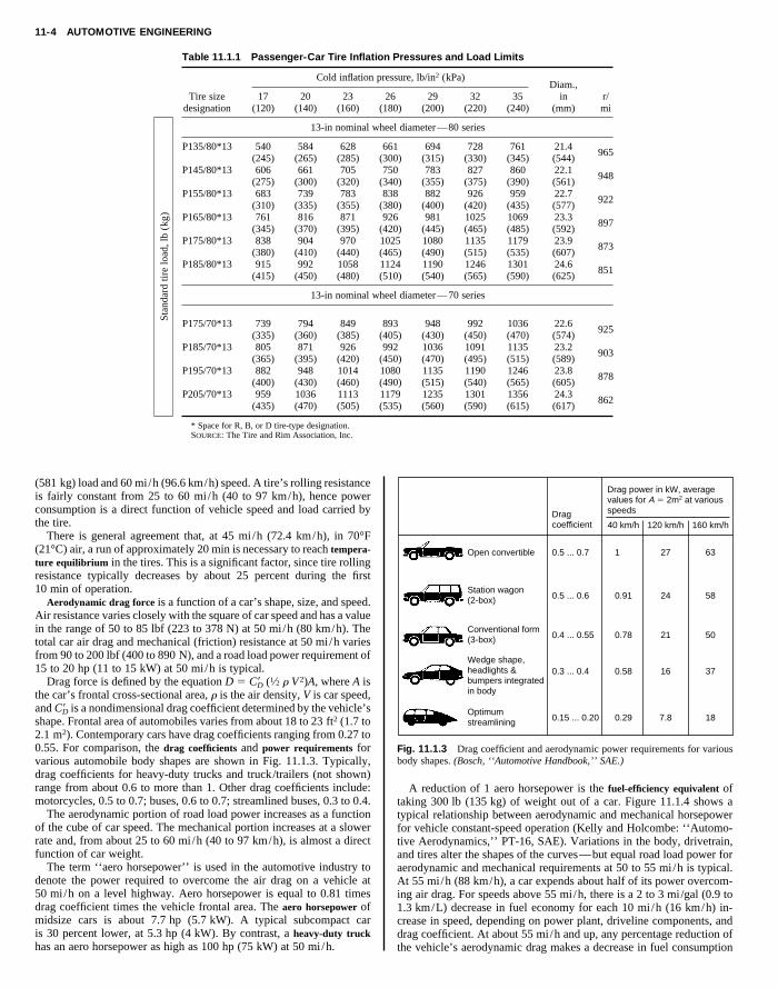
Greater tire deflection, caused by deviation from recommended loadsand air pressures (see Table 11.1.1) increases tire resistance. Low tem-peratures do likewise. Figure 11.1.2 shows the dependence of rollingresistance on inflation pressure for an FR78-14 tire tested at 1,280 lb
Fig. 11.1.2 Dependence of rolling resistance on inflation pressure for FR78-14tire, 1,280-lb load and 60-mi/h speed. (‘‘Tire Rolling Losses.’’)
11-3
11-4 AUTOMOTIVE ENGINEERING
Table 11.1.1 Passenger-Car Tire Inflation Pressures and Load Limits
Cold inflation pressure, lb/in2 (kPa)
Tire size 17 20 23 26 29 32 35Diam.,
in r/designation (120) (140) (160) (180) (200) (220) (240) (mm) mi
13-in nominal wheel diameter—80 series
P135/80*13 540 584 628 661 694 728 761 21.4965
(245) (265) (285) (300) (315) (330) (345) (544)P145/80*13 606 661 705 750 783 827 860 22.1
948(275) (300) (320) (340) (355) (375) (390) (561)
P155/80*13 683 739 783 838 882 926 959 22.7922
(310) (335) (355) (380) (400) (420) (435) (577)P165/80*13 761 816 871 926 981 1025 1069 23.3
897(345) (370) (395) (420) (445) (465) (485) (592)
P175/80*13 838 904 970 1025 1080 1135 1179 23.9873
(380) (410) (440) (465) (490) (515) (535) (607)P185/80*13 915 992 1058 1124 1190 1246 1301 24.6
851(415) (450) (480) (510) (540) (565) (590) (625)
13-in nominal wheel diameter—70 series
Stan
dard
tire
load
,lb
(kg)
P175/70*13 739 794 849 893 948 992 1036 22.6925
(335) (360) (385) (405) (430) (450) (470) (574)P185/70*13 805 871 926 992 1036 1091 1135 23.2
903(365) (395) (420) (450) (470) (495) (515) (589)
P195/70*13 882 948 1014 1080 1135 1190 1246 23.8878
(400) (430) (460) (490) (515) (540) (565) (605)P205/70*13 959 1036 1113 1179 1235 1301 1356 24.3
862(435) (470) (505) (535) (560) (590) (615) (617)
* Space for R, B, or D tire-type designation.SOURCE: The Tire and Rim Association, Inc.
(581 kg) load and 60 mi/h (96.6 km/h) speed. A tire’s rolling resistanceis fairly constant from 25 to 60 mi/h (40 to 97 km/h), hence powerconsumption is a direct function of vehicle speed and load carried bythe tire.
There is general agreement that, at 45 mi/h (72.4 km/h), in 70°F(21°C) air, a run of approximately 20 min is necessary to reach tempera-ture equilibrium in the tires. This is a significant factor, since tire rollingresistance typically decreases by about 25 percent during the first10 min of operation.
Aerodynamic drag force is a function of a car’s shape, size, and speed.
Open convertible
Station wagon
0.5 ... 0.7
0.5 ... 0.6
1
Dragcoefficient
Drag power in kW, averagevalues for A 5 2m2 at variousspeeds
40 km/h
0.91
27
120 km/h
24
63
160 km/h
58
Copyright (C) 1999 by The McGraw-Hill Companies, Inc. All rights reserved. Use ofthis product is subject to the terms of its License Agreement. Click here to view.
Air resistance varies closely with the square of car speed and has a valuein the range of 50 to 85 lbf (223 to 378 N) at 50 mi/h (80 km/h). Thetotal car air drag and mechanical (friction) resistance at 50 mi/h variesfrom 90 to 200 lbf (400 to 890 N), and a road load power requirement of15 to 20 hp (11 to 15 kW) at 50 mi/h is typical.
Drag force is defined by the equation D 5 C9D (1⁄2 r V2)A, where A isthe car’s frontal cross-sectional area, r is the air density, V is car speed,and C9D is a nondimensional drag coefficient determined by the vehicle’sshape. Frontal area of automobiles varies from about 18 to 23 ft2 (1.7 to2.1 m2). Contemporary cars have drag coefficients ranging from 0.27 to0.55. For comparison, the drag coefficients and power requirements forvarious automobile body shapes are shown in Fig. 11.1.3. Typically,drag coefficients for heavy-duty trucks and truck/trailers (not shown)range from about 0.6 to more than 1. Other drag coefficients include:motorcycles, 0.5 to 0.7; buses, 0.6 to 0.7; streamlined buses, 0.3 to 0.4.
The aerodynamic portion of road load power increases as a functionof the cube of car speed. The mechanical portion increases at a slowerrate and, from about 25 to 60 mi/h (40 to 97 km/h), is almost a directfunction of car weight.
The term ‘‘aero horsepower’’ is used in the automotive industry todenote the power required to overcome the air drag on a vehicle at50 mi/h on a level highway. Aero horsepower is equal to 0.81 timesdrag coefficient times the vehicle frontal area. The aero horsepower ofmidsize cars is about 7.7 hp (5.7 kW). A typical subcompact caris 30 percent lower, at 5.3 hp (4 kW). By contrast, a heavy-duty truckhas an aero horsepower as high as 100 hp (75 kW) at 50 mi/h.
(2-box)
Conventional form(3-box)
Optimumstreamlining
Wedge shape,headlights &bumpers integratedin body
0.4 ... 0.55
0.15 ... 0.20
0.3 ... 0.4
0.78
0.29
0.58
21
7.8
16
50
18
37
Fig. 11.1.3 Drag coefficient and aerodynamic power requirements for variousbody shapes. (Bosch, ‘‘Automotive Handbook,’’ SAE.)
A reduction of 1 aero horsepower is the fuel-efficiency equivalent oftaking 300 lb (135 kg) of weight out of a car. Figure 11.1.4 shows atypical relationship between aerodynamic and mechanical horsepowerfor vehicle constant-speed operation (Kelly and Holcombe: ‘‘Automo-tive Aerodynamics,’’ PT-16, SAE). Variations in the body, drivetrain,and tires alter the shapes of the curves—but equal road load power foraerodynamic and mechanical requirements at 50 to 55 mi/h is typical.At 55 mi/h (88 km/h), a car expends about half of its power overcom-ing air drag. For speeds above 55 mi/h, there is a 2 to 3 mi/gal (0.9 to1.3 km/L) decrease in fuel economy for each 10 mi/h (16 km/h) in-crease in speed, depending on power plant, driveline components, anddrag coefficient. At about 55 mi/h and up, any percentage reduction ofthe vehicle’s aerodynamic drag makes a decrease in fuel consumption

FUEL CONSUMPTION 11-5
of one-half or more of that same percentage. For example, for a typicalautomobile, a 10 percent reduction in aerodynamic drag yields a 5 per-cent reduction in fuel consumption at 55 mi/h.
engine crankshaft to be absorbed in accelerating the engine, drivetrainand its rotating masses, and the road wheels. For this instance, thismeans that the ‘‘effective mass’’ equals 1.33 3 actual mass.
The effective mass of engine rotating parts increases as the square ofthe engine revolutions per mile and, for a typical example, may equalor approach the car mass at a gear ratio giving about 12,000 enginerev/min. Since the effective mass of engine rotating parts increaseswith the square of the gear reduction, and the traction force increasesdirectly, there is an optimum gear reduction for maximum acceler-ation.
Copyright (C) 1999 by The McGraw-Hill Companies, Inc. All rights reserved. Use ofthis product is subject to the terms of its License Agreement. Click here to view.
Fig. 11.1.4 Vehicle road load horsepower requirements. (Four-door sedan:frontal area 22 ft2; weight 3,675 lb; CD 5 0.45.) (‘‘Automotive Aerodynamics,’’PT-78.)
Average values of traction requirements for several large cars withaverage weight (including two passengers and luggage) of 4,000 lb(1,814 kg) are shown in Fig. 11.1.5. Curves A, R, and T represent theair, rolling, and total resistance, respectively, on a level road, with nowind. Curves T9, parallel to curve T, represent the displacement of thelatter for gravity effects on the grades indicated, the additional tractionbeing equal to the car weight (4,000 lb) times the percent grade. CurveE shows the traction available in high gear in this average car. Theintersection of the ‘‘traction available’’ curve with any of the constant-gradient curves indicates the top speed that may be attained on a givengrade. For example, this hypothetical large car should negotiate a 12.5percent grade in high gear at 60 mi/h (97 km/h). Top speed on a levelgrade would be about 100 mi/h (161 km/h).
Effects of Transmission Gear Ratios Constant-horsepower parabo-las, which apply to any vehicle, are shown as light curves in Fig. 11.1.5.
Fig. 11.1.5 Traction available and traction required for a typical large automo-bile.
Except for small effects of friction losses, changes in gear ratio movepoints of a curve for traction available from an engine along theseconstant-power parabolas to traction values multiplied by the change ingear reduction. Such shifting of the traction values available from en-gines follows gear changes in the axle as well as in the gear box.
Acceleration The difference between traction force available frompower generated by an engine and the force required for constantspeed on a given grade may be used for acceleration [acceleration 521.9(100) 3 (surplus traction force/total effective car mass)], whereacceleration is in mi/h ?s, force is in lbf, and mass is in lbm.
Car weight must include a factor for the rotating parts of the engine,which may be of considerable magnitude when a high gear ratio is used.It is common for about one-third or more of the torque developed at the
The maximum acceleration rate possible is limited by the frictionbetween the driving tires and the road surface. The coefficient of fric-tion is dependent on vehicle speed, tire condition, and road conditions.At 50 mi/h (80 km/h) on a dry roadway, the coefficient of friction isabout 1.0; but, when the roadway is wet, this drops to 0.4 or lower,depending on the amount of water and the polish of the surface (‘‘BoschAutomotive Handbook,’’ 3d English ed., SAE, 1993).
For a car with 2,000 lb (907 kg) weight on the driving wheels, thelimiting traction force would be about 2,000 lbf (8,900 N) on a drypavement and less than half this value on a wet pavement. From theequation given previously, the theoretical maximum accelerations possi-ble under these two conditions for a car of 4,000 lb (1,814 kg) would beequivalent to a speed change of from 0 to 60 mi/h (97 km/h) in about5.5 and 11 s, respectively. For 0 to 60 mi/h acceleration, a roughapproximation of the time also is given by the empirical equation(Campbell, ‘‘The Sports Car,’’ Robert Bentley, Inc., 1978): t 5(2W/T)0.6, where t 5 time, s; W 5 weight, lb; T 5 maximum enginetorque, lb ? ft.
FUEL CONSUMPTION
Because motor vehicles consume more than 25 percent of the nation’sgasoline fuel and it is in the national interest to conserve energy sup-plies, the corporate average fuel economy (CAFE) of cars and truckswas regulated in 1975. Calculated according to production and saleslevel of a company’s various models, the CAFE for cars was mandatedto rise from 18 mi/gal in 1978 to 27 mi/gal in 1985 and thereafter. Forlight trucks, from 17.2 mi/gal in 1979 to 20.6 in 1995, and 20.7 in 1996.The upward trend in fuel economy is shown graphically in Figs. 11.1.6(cars) and 11.1.7 (light trucks and vans).
Vehicle design-related factors that affect fuel economy are: the vehi-cle’s purpose; performance goals; size; weight; aerodynamic drag; en-gine type, size, output, and brake specific fuel consumption; transmis-
34
32
30
28
26
24
22
20
18
16
14
12
10
Mile
s pe
r ga
llon
73 75
27.5 mpg
Import fleet
Domestic fleet
Federal standards
133.8%
1108.3%
77 79 81 83
Model year
85 87 89 91 93 95
Fig. 11.1.6 Passenger car corporate average fuel economy. (‘‘Motor VehicleFacts & Figures.’’)

11-6 AUTOMOTIVE ENGINEERING
22
20
18
allo
n2-wheel drive
4-wheel drive
Figure 11.1.8 illustrates how fuel economy is affected by designchanges such as axle ratio, engine displacement, and vehicle weight.Weight is a key determinant of fuel economy. For a rough rule-of-thumb, it may be estimated that the addition of 300 lb weight increasesfuel consumption about 1 percent (approximately 1⁄3 mi/gal for a typicalcompact car) at highway speed, and about 0.8 mi/gal in city driving. Interms of metric units, a rough estimate that evolved from Europeanengineering practice indicates that, for every 100 kg vehicle weight, 1 Lof fuel is consumed for every 100 km traveled.
Copyright (C) 1999 by The McGraw-Hill Companies, Inc. All rights reserved. Use ofthis product is subject to the terms of its License Agreement. Click here to view.
16
14
12
Mile
s pe
r g
79 81 83 85 87 89 91 93 95 97
Model year
Fig. 11.1.7 U.S. federal light truck fuel economy standards. (‘‘Motor VehicleFacts & Figures.’’)
sion type; axle ratio; tire construction; and federal standards for fueleconomy, emissions, and safety.
The principal customer- or owner-related factors include: driving pat-tern; trip length and number of stops; driving technique, especially ac-celeration, speed, and braking; vehicle maintenance; accessory opera-tion; vehicle loading; terrain; and weather. Several popular accessoriesaffect fuel economy as follows: automatic transmission, 2 to 3 mi/gal;air conditioning, 1 to 3 mi/gal; power steering, about 1⁄2 mi/gal; andpower brakes, negligible.
Fig. 11.1.8 Effect of vehicle design changes on road lo
The examples plotted in Fig. 11.1.9 for subcompact and interme-diate-size cars show fuel economy range for the urban driving cycle forengine warm and cold (short-trip). Also plotted in this graph is the roadload fuel economy variation with speed from 30 to 70 mi/h. This graphalso illustrates the general point that specific fuel consumption is thegreatest when the engine is subjected to low loads, since this is wherethe ratio between idling losses (due to friction, leaks, and nonuniformfuel distribution) and the brake horsepower is most unfavorable.
TRANSMISSION MECHANISMS
Friction clutches are either (1) the single-disk type (Fig. 11.1.10), con-necting the engine to a manual transmission, or (2) the hydraulicallyoperated multiple-disk type (Fig. 11.1.11, schematic), for control of thevarious planetary-gear changes in automatic transmissions. In (1), thearea of the friction facing is usually based on a pressure of 30 lb/in2
(206.9 kPa), and the torque rating on a friction coefficient of 0.25. Theclutch is held in engagement by several coiled springs or a diaphragmspring and is disengaged by means of a pedal with such leverage that 30to 40 lb (133 to 178 N) will overcome the clutch springs.
Fluid couplings between the engine and transmission formerly wereused to provide a smooth drive by the flow of oil between the flat radialblades in two adjacent toroidal casings (Fig. 11.1.12a, schematic). Thedifference in centrifugal force between the mass of oil contained in eachtoroid, when either is running at a speed higher than the other, causes aflow of oil from the periphery of the faster one to the slower one. Sincethis mass of oil is also rotating around the shaft at the speed of the
ad 55-mi/h fuel consumption. (Chrysler Corp.)

TRANSMISSION MECHANISMS 11-7
Fig. 11.1.9 Vehicle fuel consumption increases with speed, for subcompact and midsize cars. (Chrysler Corp.)
driving torus, its impact on the blades of the slower torus develops atorque on the latter. The developed torque is equal to, and cannot ex-ceed, the torque of the driving torus. In this respect it is similar to aslipping friction clutch. The driven member must always run at a lowerspeed, though at high rotative speeds, and when the torque demand issmall, the slip may be only 2 or 3 percent. The stalled torque increaseswith the square of the engine speed, so that very little is developed whenidling. Since torque may be transmitted in either direction, dependingonly on which member is rotating at the higher speed, the engine may beused as a brake as with friction clutches, and the car may be started by
Copyright (C) 1999 by The McGraw-Hill Companies, Inc. All rights reserved. Use ofthis product is subject to the terms of its License Agreement. Click here to view.
pushing.Torque-converter couplings (Fig. 11.1.13a) have largely replaced fluid
couplings because the torque transmitted can be increased at high slip-page. The circulation of oil between the driving, or higher-speed, torus(the pump) and the driven or lower-speed, torus (the turbine) resultsfrom the difference in centrifugal force developed in these two units,just as in the fluid coupling. With the torque converter, however, theturbine blades are given a curvature so that an additional torque isdeveloped by the reaction of a backward-spinning mass of oil as itleaves the turbine. Stationary, or stator, blades are interposed betweenthe turbine and the pump to change the direction of the oil spin. Theentrance angle of the stator blades required for tangential flow varies
Fig. 11.1.10 Single-plate dry-disk friction clutch.
Fig. 11.1.11 Schematic of two hydraulically operated multiple-disk clutches inan automatic transmission. (Ford Motor Co.)
(a) (b)
Fig. 11.1.12 Fluid coupling: (a) section; (b) characteristics.
widely with the slip ratio. For a given blade angle there is a hydraulicshock loss at any slip ratio greater or less than that which providestangential flow. This is reflected in the rapid fall of the efficiency curvein Fig. 11.1.14b on each side of the maximum. The essential parts of atorque converter with its stationary stator are shown in Fig. 11.1.14a. Astalled-torque multiplication of 2.0 to 2.7 is used in various designs.

11-8 AUTOMOTIVE ENGINEERING
When the torque ratio is almost unity, the slip is such that oil from theturbine starts to impinge on the back of the stator blades. By mountingthe stator assembly on a sprag, or one-way clutch (Fig. 11.1.13a),it remains stationary while subject to the reversing action of the
Figure 11.1.15 compares a torque-converter coupling to a frictionclutch on car performance in direct drive. The increase in tractionavailable for acceleration from a standing start substantiates its publicacceptance. An axle gear is generally used which gives a propeller shaftspeed about 90 percent as great as with a manual transmission at thesame car speed. The gain in engine efficiency compensates for thelosses of the automatic transmissions under steady cruising speeds.
Copyright (C) 1999 by The McGraw-Hill Companies, Inc. All rights reserved. Use ofthis product is subject to the terms of its License Agreement. Click here to view.
(a)
(b)Fig. 11.1.13 Torque convertercoupling: (a) section; (b) character-istics.
backward-spinning oil mass as it leaves the turbine. When the slipreaches the point where the oil flow from the turbine begins to spin for-ward, the stator is free to turn with it. When the slip is further reduced,the unit acts as a fluid coupling with improved efficiency (Fig.11.1.13b). Such a unit is a fluid torque-converter coupling. Some designs
Fig. 11.1.14 Torque converter:(a) section; (b) characteristics.
eliminate slippage by the inclusion of a friction clutch which carries theload when a predetermined car speed is reached. These clutches arehydraulically operated, the engagement being controlled automaticallyby accelerator position and car speed.
Fig. 11.1.16 Three-speed synchromesh transmission. (B
Fig. 11.1.15 Comparative traction available in the performance of a fluidtorque-converter coupling and a friction clutch.
However, there may be a considerable loss of power during accelerationunless supplemented by such modifications as one or more auxiliarygear ratios or variable-angle stator vanes. Various design modifi-cations of torque-converter couplings have been introduced by differentmanufacturers, such as two or more stators, each independentlymounted on one way clutches, and variable pitch angles for the statorblades. These provide compromises in blade angles for the developmentof rapid acceleration without sacrifice of high efficiency whilecruising.
Manual transmissions installed as standard equipment on Americancars have three, four, or five forward speeds, including direct drive, andone reverse. These speeds are obtained by sliding either one of twogears along a splined shaft to bring it into mesh with a correspondinggear on a countershaft which is, in turn, driven by a pair of gears inconstant mesh. Helical gears are used to minimize noise. A ‘‘synchro-mesh’’ device (Fig. 11.1.16), acting as a friction clutch, brings the gearsto be meshed approximately to the correct speed just before meshingand minimizes ‘‘clashing,’’ even with inexperienced drivers. Gear
uick.)

AUTOMATIC TRANSMISSIONS 11-9
Fig. 11.1.17 Planetary gear action: (a) Large speed reduction: ratio 5 1 1 (internal gear diam.)/(sun gear diam.) 53.33 for example shown. (b) Small speed reduction: ratio 5 1 1 (sun gear diam.)/(internal gear diam.) 5 1.428.(c) Reverse gear ratio 5 (internal gear diam.)/(sun gear diam.) 5 2 2.33.
changes are generally in geometric ratios. Transmission ratios averageabout 2.76 in first gear, 1.64 in second, 1.0 in third or direct drive, and3.24 in reverse. The shift lever is generally located on the steeringcolumn. Four-speed transmissions usually have the shift lever on thefloor. Average gear ratios are about 2.67 in first, 1.93 in second, 1.45 inthird, and 1.0 in fourth or direct drive.
Overdrives have been available for some cars equipped with manualtransmissions. These are supplemental planetary gear units with threeplanetary pinions driven around a stationary sun gear. The surroundinginternal gear is coupled to the propeller shaft, which thus turns faster
and the forward internal gear carries the planets of the rear unit. Theinternal gears of both systems are all of the same size, and consequentlyall planets are of equal size. This arrangement, together with threeclutches, two brake bands, and suitable one-way sprags, makes possiblethree forward gear or torque ratios, plus direct drive and reverse.
Many automatic transmissions use a lockup clutch to improve per-formance and fuel economy. The torque converter is used for power andsmoothness while accelerating in first and second gears until road speedreaches about 40 mi/h (64 km/h). Then, after the transmission upshiftsfrom second to third gear, the clutch automatically locks up the torque
Copyright (C) 1999 by The McGraw-Hill Companies, Inc. All rights reserved. Use ofthis product is subject to the terms of its License Agreement. Click here to view.
than the engine. The gear ratio is selected to permit the engine to slowdown to about 70 percent of the propeller-shaft speed and operate withless noise and friction. These units automatically come into action whenthe driver momentarily releases the accelerator pedal at a car speedabove 25 to 28 mi/h (40 to 45 km/h).
AUTOMATIC TRANSMISSIONS
Automatic transmissions commonly use torque-converter couplingswith planetary-gear units that can supply one or two gear reductions andreverse, depending on the design, by simultaneously engaging or lock-ing various elements of planetary systems (Fig. 11.1.17). Automaticcontrol is provided by disk clutches or brake bands which lock thevarious elements, operated by oil pressure as regulated by governors atcar speeds where shifts are made from one speed to another.
A schematic of a representative automatic transmission, combining athree-element torque converter and a compound planetary gear is shownin Fig. 11.1.18. The speed reductions and reverse are provided by acompound planetary system consisting of two simple systems in series.The two sun gears are an integral unit with the same number of teeth,
Fig. 11.1.18 Three-element torque converter and p
converter so there is a direct mechanical drive through the transmission.Normal slippage in the converter is eliminated, engine speed is reduced,and fuel economy is improved. The lockup clutch disengages automati-cally during part-throttle or full-throttle downshifts and, when the vehi-cle is slowed, to a speed slightly below the lockup speed.
Approximately two-thirds of 1995 cars have electronically controlledautomatic transmissions. Combined electronic-hydraulic units for con-trol of automatic transmissions are, increasingly, superseding systemsthat rely solely on hydraulic control. Hydraulic actuation is retained forthe clutches, while electronic modules assume control functions for gearselection and for modulating pressure in accordance with torque flow.Sensors monitor load, selector-lever position, program, and kick-downswitch positions, along with rotational speed at both the engine andtransmission shafts. The control unit processes these data to producecontrol signals for the transmission. Advantages include: diverse shiftprograms, smooth shifts, flexibility for various vehicles, simplified hy-draulics, and elimination of one-way clutches.
Worldwide, automatic transmission engineering practice includessome evolving design development and growing production acceptanceof continuously variable transmissions (CVT). The CVT can convert the
lanetary gear. (General Motors Corp.)

11-10 AUTOMOTIVE ENGINEERING
engine’s continuously varying operating curve to an operating curve ofits own, and every engine operating curve into an operating range withinthe field of potential driving conditions. The theoretical advantage (overfixed-ratio transmissions) lies in a potential for enhancing vehicle per-formance and fuel economy while reducing exhaust emissions. This isdone by maintaining the engine in a performance range for best fueleconomy. There are, however, practical limitations and consider-ations that constrain the full exploitation of the CVT’s theoretical capa-bilities.
The CVT can operate mechanically (belt or friction roller), hydrauli-
are offered as optional equipment on most cars. One design has fourpinions which are carried on two separate cross shafts at right angles toeach other, each being driven by V-shaped notches in the carrier. Astorque is developed to drive either axle, one pinion cross shaft or theother moves axially and locks the corresponding disk-clutch plates be-tween that axle drive gear and the differential housing. In another de-sign, similar disk clutches are locked by spring pressure, which preventsdifferential action until a differential torque greater than the limit estab-lished by the springs is developed.
The semifloating rear axle (Fig. 11.1.20) used on many rear-wheel
Copyright (C) 1999 by The McGraw-Hill Companies, Inc. All rights reserved. Use ofthis product is subject to the terms of its License Agreement. Click here to view.
cally, or electrically. Currently, the highest level of development hasbeen attained with mechanical continuously variable designs using steelbelts. A general feature of CVT is manipulation of engine speed, withthe objective of maintaining constant engine speed; or optimizing en-gine speed changes in response to changing driving conditions. CVTdevelopmental activity includes: high-torque and high-speed belts, elec-tronic control for line pressure and engine speed, torque converters withelectronically controlled lockup clutch, and roller vane pumps withelectronically operated flow control valve.
FINAL DRIVE
The differential is a unit attached to the ring gear (Figs. 11.1.19 and11.1.20) which equalizes the traction of both wheels and permits onewheel to turn faster than the other, as needed on curves. Each axle isdriven by a bevel gear meshing with pinions on a cross-shaft pinion pin
Fig. 11.1.19 Rear-axle hypoid gearing.
secured to the differential case. The case also carries the ring gear. Anundesirable feature of the conventional differential is that no more trac-tion may be developed on one wheel than on the other. If one wheelslips on ice, there is no traction to move the car. Limited-slip differentials
Fig. 11.1.20 Rear axle. (Oldsmobile.)
drive cars has a bearing for each drive axle at the outer end of thehousing as well as near the differential carrier, with the full load on eachwheel taken by the drive axles in combined bending and shear. Thefull-floating axle, generally used on commercial vehicles, supports eachwheel on two bearings carried by the axle housing or an extension to it.Each wheel is bolted to a flange on one of the axle shafts. The axleshafts carry none of the vehicle weight and may be withdrawn withoutjacking up the wheel.
The front-wheel drive (FWD) cars commonly use a transaxle that com-bines a torque converter, automatic three-speed or four-speed transmis-sion, final drive gearing, and differential into a compact drive system,such as illustrated in the cutaway view shown in Fig. 11.1.21. Typically,the torque converter, transaxle unit, and differential are housed in anintegral aluminum die casting. The differential oil sump is separatefrom the transaxle sump. The torque converter is attached to the crank-shaft through a flexible driving plate. The converter is cooled by circu-lating the transaxle fluid through an oil-to-water type cooler, located inthe radiator side tank.
Engine torque is transmitted to the torque converter through the inputshaft to multiple disk clutches in the transaxle. The power flow dependson the application of the clutches and bands. As illustrated in Fig.11.1.22, the transaxle consists of two multiple-disk clutches, anoverrunning clutch, two servos, a hydraulic accumulator, two bands,and two planetary gear sets, to provide three or four forward ratios and areverse ratio.
The common sun gear of the planetary gear sets is connected to thefront clutch by a driving shell that is splined to the sun gear and to thefront clutch retainer. The hydraulic system consists of an oil pump and asingle valve body that contains all of the valves except the governorvalves.
Output torque from the main centerline is delivered through helicalgears to the transfer shaft. This gear set is a factor in the final drive(axle) ratio. The shaft also carries the governor and the parking sprag.An integral helical gear on the transfer shaft drives the differential ringgear. In a representative FWD vehicle, the final drive gearing is com-pleted with either of two gear sets to produce overall ratios of 3.48, 3.22,and 2.78.
SUSPENSIONS 11-11
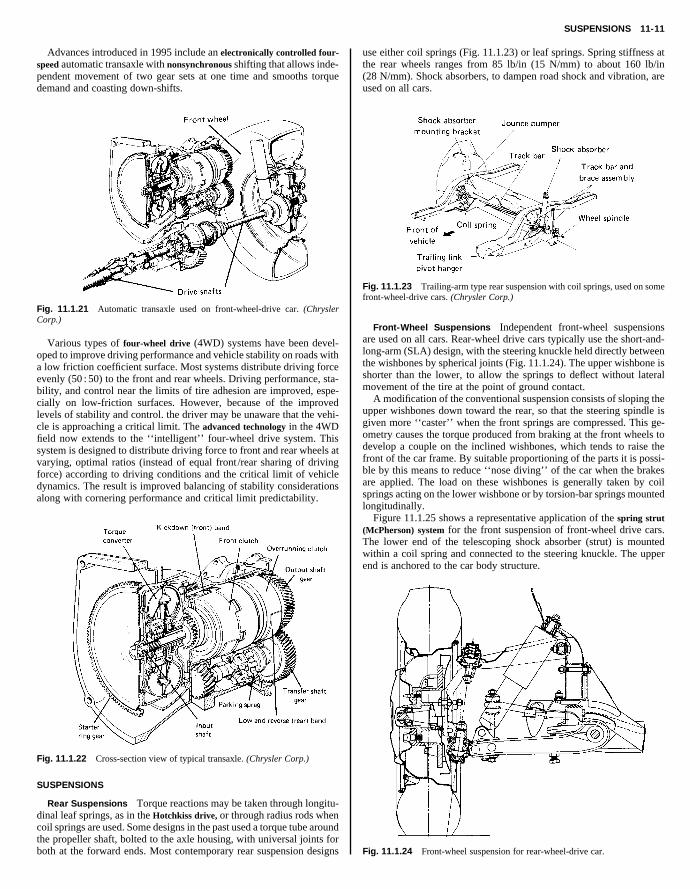
Advances introduced in 1995 include an electronically controlled four-speed automatic transaxle with nonsynchronous shifting that allows inde-pendent movement of two gear sets at one time and smooths torquedemand and coasting down-shifts.
use either coil springs (Fig. 11.1.23) or leaf springs. Spring stiffness atthe rear wheels ranges from 85 lb/in (15 N/mm) to about 160 lb/in(28 N/mm). Shock absorbers, to dampen road shock and vibration, areused on all cars.
Copyright (C) 1999 by The McGraw-Hill Companies, Inc. All rights reserved. Use ofthis product is subject to the terms of its License Agreement. Click here to view.
Fig. 11.1.21 Automatic transaxle used on front-wheel-drive car. (ChryslerCorp.)
Various types of four-wheel drive (4WD) systems have been devel-oped to improve driving performance and vehicle stability on roads witha low friction coefficient surface. Most systems distribute driving forceevenly (50 : 50) to the front and rear wheels. Driving performance, sta-bility, and control near the limits of tire adhesion are improved, espe-cially on low-friction surfaces. However, because of the improvedlevels of stability and control. the driver may be unaware that the vehi-cle is approaching a critical limit. The advanced technology in the 4WDfield now extends to the ‘‘intelligent’’ four-wheel drive system. Thissystem is designed to distribute driving force to front and rear wheels atvarying, optimal ratios (instead of equal front /rear sharing of drivingforce) according to driving conditions and the critical limit of vehicledynamics. The result is improved balancing of stability considerationsalong with cornering performance and critical limit predictability.
Fig. 11.1.22 Cross-section view of typical transaxle. (Chrysler Corp.)
SUSPENSIONS
Rear Suspensions Torque reactions may be taken through longitu-dinal leaf springs, as in the Hotchkiss drive, or through radius rods whencoil springs are used. Some designs in the past used a torque tube aroundthe propeller shaft, bolted to the axle housing, with universal joints forboth at the forward ends. Most contemporary rear suspension designs
Fig. 11.1.23 Trailing-arm type rear suspension with coil springs, used on somefront-wheel-drive cars. (Chrysler Corp.)
Front-Wheel Suspensions Independent front-wheel suspensionsare used on all cars. Rear-wheel drive cars typically use the short-and-long-arm (SLA) design, with the steering knuckle held directly betweenthe wishbones by spherical joints (Fig. 11.1.24). The upper wishbone isshorter than the lower, to allow the springs to deflect without lateralmovement of the tire at the point of ground contact.
A modification of the conventional suspension consists of sloping theupper wishbones down toward the rear, so that the steering spindle isgiven more ‘‘caster’’ when the front springs are compressed. This ge-ometry causes the torque produced from braking at the front wheels todevelop a couple on the inclined wishbones, which tends to raise thefront of the car frame. By suitable proportioning of the parts it is possi-ble by this means to reduce ‘‘nose diving’’ of the car when the brakesare applied. The load on these wishbones is generally taken by coilsprings acting on the lower wishbone or by torsion-bar springs mountedlongitudinally.
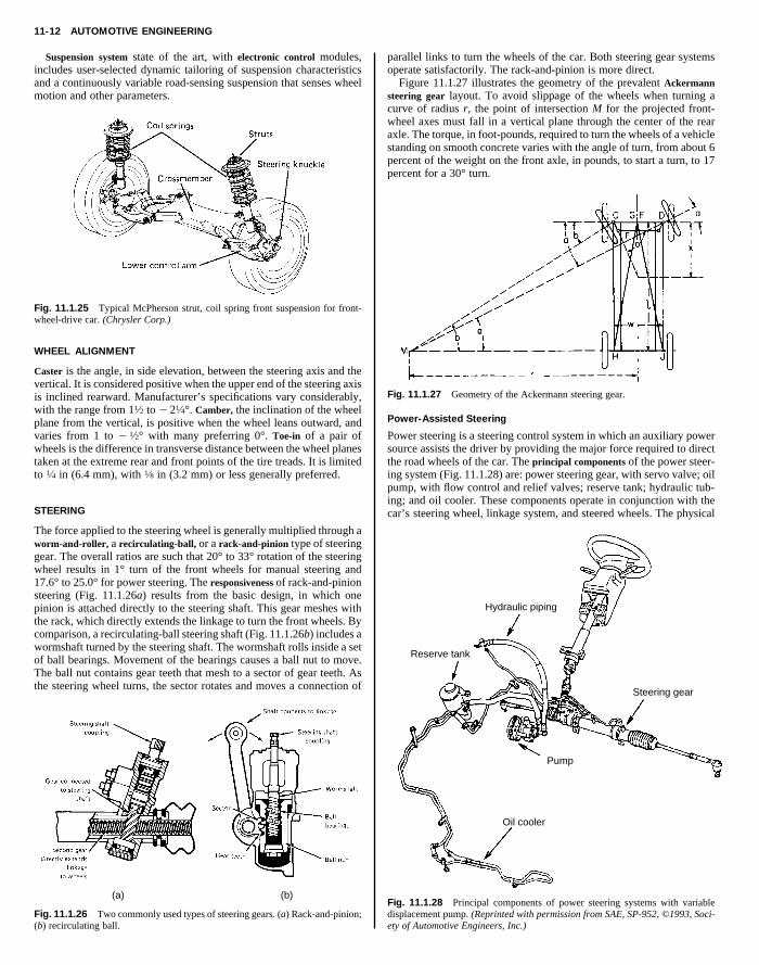
Figure 11.1.25 shows a representative application of the spring strut(McPherson) system for the front suspension of front-wheel drive cars.The lower end of the telescoping shock absorber (strut) is mountedwithin a coil spring and connected to the steering knuckle. The upperend is anchored to the car body structure.
Fig. 11.1.24 Front-wheel suspension for rear-wheel-drive car.
11-12 AUTOMOTIVE ENGINEERING
Suspension system state of the art, with electronic control modules,includes user-selected dynamic tailoring of suspension characteristicsand a continuously variable road-sensing suspension that senses wheelmotion and other parameters.
parallel links to turn the wheels of the car. Both steering gear systemsoperate satisfactorily. The rack-and-pinion is more direct.
Figure 11.1.27 illustrates the geometry of the prevalent Ackermannsteering gear layout. To avoid slippage of the wheels when turning acurve of radius r, the point of intersection M for the projected front-wheel axes must fall in a vertical plane through the center of the rearaxle. The torque, in foot-pounds, required to turn the wheels of a vehiclestanding on smooth concrete varies with the angle of turn, from about 6percent of the weight on the front axle, in pounds, to start a turn, to 17percent for a 30° turn.
Copyright (C) 1999 by The McGraw-Hill Companies, Inc. All rights reserved. Use ofthis product is subject to the terms of its License Agreement. Click here to view.
Fig. 11.1.25 Typical McPherson strut, coil spring front suspension for front-wheel-drive car. (Chrysler Corp.)
WHEEL ALIGNMENT
Caster is the angle, in side elevation, between the steering axis and thevertical. It is considered positive when the upper end of the steering axisis inclined rearward. Manufacturer’s specifications vary considerably,with the range from 11⁄2 to 2 21⁄4°. Camber, the inclination of the wheelplane from the vertical, is positive when the wheel leans outward, andvaries from 1 to 2 1⁄2° with many preferring 0°. Toe-in of a pair ofwheels is the difference in transverse distance between the wheel planestaken at the extreme rear and front points of the tire treads. It is limitedto 1⁄4 in (6.4 mm), with 1⁄8 in (3.2 mm) or less generally preferred.
STEERING
The force applied to the steering wheel is generally multiplied through aworm-and-roller, a recirculating-ball, or a rack-and-pinion type of steeringgear. The overall ratios are such that 20° to 33° rotation of the steeringwheel results in 1° turn of the front wheels for manual steering and17.6° to 25.0° for power steering. The responsiveness of rack-and-pinionsteering (Fig. 11.1.26a) results from the basic design, in which onepinion is attached directly to the steering shaft. This gear meshes withthe rack, which directly extends the linkage to turn the front wheels. Bycomparison, a recirculating-ball steering shaft (Fig. 11.1.26b) includes awormshaft turned by the steering shaft. The wormshaft rolls inside a setof ball bearings. Movement of the bearings causes a ball nut to move.The ball nut contains gear teeth that mesh to a sector of gear teeth. Asthe steering wheel turns, the sector rotates and moves a connection of
(b)(a)
Fig. 11.1.26 Two commonly used types of steering gears. (a) Rack-and-pinion;(b) recirculating ball.
Fig. 11.1.27 Geometry of the Ackermann steering gear.
Power-Assisted Steering
Power steering is a steering control system in which an auxiliary powersource assists the driver by providing the major force required to directthe road wheels of the car. The principal components of the power steer-ing system (Fig. 11.1.28) are: power steering gear, with servo valve; oilpump, with flow control and relief valves; reserve tank; hydraulic tub-ing; and oil cooler. These components operate in conjunction with thecar’s steering wheel, linkage system, and steered wheels. The physical
Hydraulic piping
Reserve tank
Oil cooler
Pump
Steering gear
Fig. 11.1.28 Principal components of power steering systems with variabledisplacement pump. (Reprinted with permission from SAE, SP-952, ©1993, Soci-ety of Automotive Engineers, Inc.)

BRAKES 11-13
effort required to steer an automobile, especially when parking, is ap-preciably lessened by the power-assisted steering device. This permitsreduction in the gear ratio between the steering wheel and the car wheelsfrom some 30 to 15, with consequent reduction in the number of turns ofthe steering wheel for the complete movement of the front wheels fromextreme right to left from 5.5 to 3. Power-assisted steering has beenoffered for many years on U.S. cars as standard or optional equipment.Public acceptance is such that 88 percent of the cars sold in 1993 wereso equipped.
All systems provide (1) steering control in case of failure of the
Three types of rotary pumps for the high pressures required are shownin Fig. 11.1.30 (see also Sec. 14.1). Centrifugal force holds the slidingelements against a cam-shaped or eccentric case at high speeds. At lowspeeds, the sliding elements are held against the case—in design a bysprings and in design c by oil pressure admitted to the base of the vanes.The double cam of design c, in addition to doubling the normal volu-metric displacement, provides for balancing the oil pressure on eachside of the rotor and on the bearings. The cam is contoured for uniformacceleration.
Copyright (C) 1999 by The McGraw-Hill Companies, Inc. All rights reserved. Use ofthis product is subject to the terms of its License Agreement. Click here to view.
hydraulic-power assistance, and (2) a ‘‘feel of the road,’’ by which thedriver’s effort on the steering wheel is proportional to the force neededto turn the front wheels and by which the tendency of a car to straightenout from a turn or the drag of a soft front tire may be felt at the steeringwheel.
Power assistance is effected by hydraulic pressure from an engine-drive pump, acting on a piston in the steering linkage. The piston and itscylinder are incorporated in the steering-gear housing. Oil pressure onthe piston is controlled by a valve, such as the balanced spool valve ofFig. 11.1.29.
Fig. 11.1.29 Control valve positioned for full-turn power steering assistanceusing maximum pump pressure.
When the spool is moved slightly to the right, lands on the spoolrestrict the return of oil from the pump through both return circuits, thusbuilding up delivery pressure. Since the pump delivery is still open tothe left end of the power cylinder while the right end is open to the pumpsuction, a force is developed to move the piston to the right. The greaterthe restriction imposed on the return of oil to the pump, the greater willbe the pressure and the resulting force on the piston.
The spool is centered to the neutral position by suitable centeringsprings. These provide an increasing effort on the steering wheel forincreasing steering angle. Although they aid in straightening out from aturn, they do not give the driver a feel of the force required to providethe steering direction. Hydraulic reaction against the spool, which is feltat the steering wheel and is proportional to the force developed by thesteering gear, is developed by subjecting the ends of the spool to the oilpressure on either side of the power piston.
The valve is held in its neutral position by preloading the centeringsprings. Steering effort at the wheel overcomes this preload. Duringnormal, straight-highway driving, the steering effort is less than thepreload and there is no hydraulic assistance; the steering gear is freelyreversible, and the driver can ‘‘feel the road’’ and correct for elementssuch as road camber and crosswinds. The caster action of the frontwheels straightens the path of the car when it is coming out of a turn.Any steering effort greater than the preload of the centering springsallows the spool movement to develop a steering assistance proportionalto the steering effort and to correspondingly reduce, but not eliminate,the road reactions and shocks felt by the driver.
Oil pumps for power-assisted steering gears are generally driven fromthe engine by belts, though in some instances they have been driven athigher speeds directly from the electric generator. A typical unit deliv-ers 1.75 gal/min (6.62 L/min) at engine idling speed, at any pressure upto 1,200 lb/in2 (8.3 MPa) as may be required while parking.
Fig. 11.1.30 Rotary pump types: (a) Chrysler; (b) Ford (Eaton); (c) GeneralMotors (Saginaw).
Variable displacement vane pumps (instead of fixed displacement) areused to raise the efficiency of power steering systems. The variabledisplacement design reduces power consumption by curtailing the surplusoil flow at the middle and high revolution speeds of the steering appa-ratus. The amount of oil that is pumped is matched to the requirementsof the system in its various operating stages.
BRAKES
Stopping distance— the distance traveled by a vehicle after an obstaclehas been spotted until the vehicle is brought to a halt—is the sum of thedistances traveled during the reaction time and the braking time.
The braking ratio z, usually expressed as a percentage, is the ratiobetween braking deceleration and the acceleration due to gravity (g 532.2 ft/s2 or 9.8 m/s2). The upper and lower braking ratio values arelimited by static friction between tire and road surface and the legallyprescribed values for stopping distances.
The reaction time is the time that elapses between the driver’s percep-tion of an object and commencement of action to apply the brakes. Thistime is not constant; it varies from 0.3 to 1.7 s, depending on personaland external factors. For a reaction time of 1 s, Table 11.1.2 givesstopping distances for various speeds and values of braking ratio (de-celeration rates).
The maximum retarding force that can be applied to a vehicle throughits wheels is limited by the friction between the tires and the road, equalto the coefficient of friction times the vehicle weight. With a coefficientof 1.0, which is about the maximum for dry pavement, this force canequal the car weight and can develop a retardation of 1.0 g. In thisinstance, stopping distance S 5 V2/29.9, where V is in mi/h and S isexpressed in feet. For metric units, where S is meters and V is km/h, theequation is S 5 V2/254.
For typical vehicle, tire, and road conditions, with a 0.4 coefficientof friction, 0.4 g deceleration rate, and a reaction time of 1 s, the follow-ing is a rule-of-thumb equation for stopping distance; S ' (V/10)2 1(3V/10), where S is stopping distance in meters and V is thespeed in km/h.

11-14 AUTOMOTIVE ENGINEERING
Table 11.1.2 Stopping Distances (Calculated)
Driving speed before applying brakes, mi/h (km/h)
Braking ratio z, 12 25 31 37 43 50 56 62 69 75% (20) (40) (50) (60) (70) (80) (90) (100) (110) (120)
Reaction distance traveled in 1 s (no braking), ft (m)
18 36 46 56 62 72 82 92 102 108(5.6) (11) (14) (17) (19) (22) (25) (28) (31) (33)
Stopping distance (reaction 1 braking), ft (m)
30 36 105 151 207 269 344 427 509 607 705(11) (32) (46) (63) (82) (105) (130) (155) (185) (215)
50 29 75 108 148 187 233 285 344 410 476(8.7) (23) (33) (45) (57) (71) (87) (105) (125) (145)
70 26 66 92 121 151 187 230 272 318 360(7.8) (20) (28) (37) (46) (57) (70) (83) (97) (110)
90 24 53 82 105 131 164 197 233 272 312(7.3) (18) (25) (32) (40) (50) (60) (71) (83) (95)
SOURCE: Bosch, ‘‘Automotive Handbook,’’ SAE.
The automobile’s brake system is based on the principles of hydraulics.Hydraulic action begins when force is applied to the brake pedal. Thisforce creates pressure in the master cylinder, either directly or through apower booster. It serves to displace hydraulic fluid stored in the mastercylinder. The displaced fluid transmits the pressure through the fluid-filled brake lines to the wheel cylinders that actuate the brake shoe (orpad) mechanisms. Actuation of these mechanisms forces the brake padsand linings against the rotors (front wheels) or drums (rear wheels) tostop the wheels.
All automobiles have two independent systems of brakes for safety.
original positions. This uncovers the compensating ports, permittingbrake fluid to enter from the reservoir or to escape from the wheelcylinders after brake application. The check valve facilitates the main-tenance of 8 to 16 lb/in2 (55 to 110 kPa) line pressure to prevent theentrance of air into the system.
Copyright (C) 1999 by The McGraw-Hill Companies, Inc. All rights reserved. Use ofthis product is subject to the terms of its License Agreement. Click here to view.
One is generally a parking brake and is rarely used to stop a car fromspeed, though it should be able to. The brake manually operates on therear wheels through cables or mechanical linkage from an auxiliary footlever (or a hand pull); it is held on by a ratchet until released by somemeans such as a push button or a lever.
The main system, or service brakes, on all U.S. cars is hydraulicallyoperated, with equalized pressure to all four wheels, except with diskbrakes on front wheels, where a proportioning valve is used to permitincreased pressure to the disk calipers. Rubber seals preclude the use ofpetroleum products; hydraulic fluids are generally mixtures of glycolswith inhibitors. Figure 11.1.31 shows the split system, for improved
Fig. 11.1.31 ‘‘Split’’ hydraulic brake system.
safety, with two independent master cylinders in tandem, each actuatinghalf the brakes, either front or rear or one front and the opposite rear.Failure of either hydraulic section allows stopping of the car by brakeson two wheels.
Figure 11.1.32 shows the customary design of a brake dual mastercylinder by which the brake shoes are applied in the conventionalinternal-expanding brakes (Fig. 11.1.33). When the brakes arereleased, a spring in the master cylinder returns the pistons to their
Fig. 11.1.32 Typical design of a dual master cylinder for a split brake system.
Three types of internal-expanding brakes (Fig. 11.1.33) have been ac-cepted in service. All are self-energizing, where the drum rotation in-creases the applying force supplied by the wheel cylinder.
With the trailing shoe (Fig. 11.1.33a), friction is opposed to the actu-ating force. The resulting deenergizing of this shoe causes it to do aboutone-third the work of the leading shoe. Its tendency to lock or squeal isless, and the length and position of the lining are not so critical. The typeof brake shown in Fig. 11.1.33a, with one leading and one trailing shoe,formerly was used for the rear wheels. The braking work and wear ofthe two shoes can be equalized by use of a larger bore for that half of thewheel cylinder which operates the trailing shoe.
The design shown in Fig. 11.1.33b has two leading shoes, each ac-tuated by a single-piston wheel cylinder and each self-energizing. Thisdesign has been used for the front wheels where the Fig. 11.1.33a de-sign was used for the rear wheels.
Figure 11.1.33c shows the Bendix Duo-Servo design, used on manycars, in which the self-energizing action of two leading shoes is muchincreased by turning them ‘‘in series’’; the braking force developed bythe primary shoe becomes the actuating force for the secondary shoe.The action reverses with rotation.
Adjustment for lining wear is effected automatically on most cars. Ifsufficient wear has developed, a linkage may turn the notched wheel onthe adjusting screw (Fig. 11.1.33c) by movement of the primary shoerelative to the anchor pin when the brake is applied with the car movingin reverse. On other designs, adjustment is by linkage between the handbrake and the adjusting wheel.
Brake drums are designed to be as large as practicable in order todevelop the necessary torque with the minimum application effort and

BRAKES 11-15
Fig. 11.1.33 Three types of internal-expanding brakes.
to limit the temperature developed in dissipating the heat of friction.The 14- and 15-in (36- and 38-cm) wheel-rim diameters limit the drumdiameters to 10 to 12 in (25 to 30 cm), and the 13-in (33-cm) rims limitthe diameters to 8 to 91⁄2 in (20 to 24 cm). Drum widths limit unitpressures between the linings and the drums to 16 to 23 lb (7.2 to10.4 kg) of car weight per in2. Drum friction surfaces are usually castiron or iron alloy. Drum brake shoes and disk brake caliper pads are linedwith compounds of resin, metal powder, solid lubricant, abrasives, or-ganic and inorganic fillers, and fibers. Environmental concerns led tothe development of asbestos-free brake system friction materials. These
ment on virtually all car models. The supplemental force is developedon a diaphragm by vacuum from the engine intake manifold, eithermechanically to the master cylinder or hydraulically, to boost (1) theforce between the pedal and the master cylinder, or (2) the hydraulicpressure between the master cylinder and the brakes. Common charac-teristics are (1) a braking force which is related to pedal pressure so thatthe driver can feel a pedal reaction proportional to the force applied, and(2) ability to apply the brakes in the absence of the supplemental power.
Figure 11.1.35 illustrates a passenger-car vacuum-suspended type ofpower brake, where vacuum exists on both sides of the main power
Copyright (C) 1999 by The McGraw-Hill Companies, Inc. All rights reserved. Use ofthis product is subject to the terms of its License Agreement. Click here to view.
materials take into account the full range of brake performance require-ments, including the mechanism of brake noise and the causes for brakejudder (abnormal vibration), and squeal. Current nonasbestos, nonsteelfriction materials for brake linings and pads include those with mainfibers of carbon and aramid plastic. Secondary fibers are copper andceramic. Friction coefficients range from 0.3 to 0.4.
Where identical brakes are used on front and rear wheels, the rear-wheel cylinders are smaller, so that about 40 to 45 percent of totalbraking force is developed at the rear wheels. With the split system (Fig.11.1.31), a smaller master cylinder for the rear brakes gives a similardivision. Master cylinders are about 1 in (25.4 mm) in diameter, andother parts of the brake system are so proportioned that a 100-lb (445-N)brake-pedal force develops 600- to 1,200-lb/in2 (4.1- to 8.3-MPa) fluidpressure. Air in a hydraulic system makes the brakes feel spongy, and itmust be bled wherever it accumulates, as at each wheel cylinder.
Caliper disk brakes (Fig. 11.1.34) offer better heat dissipation by di-rect contact with moving air; they are not self-energizing, so that there is
Fig. 11.1.34 Caliper disk brake (schematic).
less drop in the friction coefficient with temperature rise of the brakepads. Contrarily, the absence of self-energization requires higherhydraulic-system pressures and consequent power boosters on heaviercars. Wear of the friction pads is normally greater because of the smallerarea of contact and the greater exposure to road dirt. The pads areconsequently made thicker than the linings of drum brakes, and auto-matic retraction is incorporated in the hydraulic cylinders.
Power-assisted brakes relieve the driver of much physical effort inretarding or stopping a car. They are either standard or optional equip-
element when the brakes are released. In the released position, there iscontact between the valve plunger and the poppet; thus the port is closedbetween the power cylinder and the atmosphere.
Fig. 11.1.35 Power-assisted brake installation.
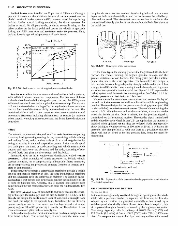
Physical effort applied to the brake pedal moves the valve operatingrod toward the master-cylinder section. Initial movement of this rodcloses the port between the poppet and the power piston. This closes thevacuum passage and brings the valve plunger into contact with theresilient reaction disk. Additional movement of the valve rod then sepa-rates the valve plunger from the poppet, thus opening the atmosphericport and admitting air to the control chamber. Air pressure in thischamber depends upon the amount of physical effort applied to the pedal.The pressure differences between the two sides of the power pistoncause it to move toward the master cylinder, closing the vacuum portand transferring its force through the reaction disk to the hydraulicpiston of the master cylinder. This force tends to extrude the reactiondisk against the valve plunger and react against the valve operating rod,thus reducing the pedal effort required. An inherent feature of thevacuum-suspended type of power brake is the existence of vacuum,without an additional reservoir, for at least one brake stop after theengine is stopped. Figure 11.1.36 shows the relationship between pedaleffort and hydraulic line pressure.
11-16 AUTOMOTIVE ENGINEERING
Antilock brakes were installed on 56 percent of 1994 cars. On eightpercent of these cars, the additional feature of traction control was in-cluded. Antilock brake systems (ABS) prevent wheel lockup duringbraking. Under normal braking conditions, the driver operates thebrakes as usual. On slippery roads, or during severe braking, as thedriver pushes on the brake pedal and causes the wheels to approachlockup, the ABS takes over and modulates brake line pressure. Thus,braking force is applied independently of pedal force.
the plies do not cross one another. Reinforcing belts of two or morelayers are laid circumferentially around the tire between the radial bodyplies and the tread. The bias-belted tire construction is similar to theconventional bias-ply tire, but it has circumferential belts like those inthe radial tire.
Copyright (C) 1999 by The McGraw-Hill Companies, Inc. All rights reserved. Use ofthis product is subject to the terms of its License Agreement. Click here to view.
Fig. 11.1.36 Performance chart of a typical power-assisted brake.
Traction control functions as an extension of antilock brake systems,with which it shares numerous components. Traction control helpsmaintain directional stability along with good traction. An ABS systemwith traction control uses brake applications to control slip. The amountof force transferred when starting off or during deceleration or accelera-tion is a function of the amount of slip between the tire and the road. Thecombined antilock and traction control systems make extensive use ofautomotive electronics including elements such as sensors (to measurewheel angular velocity), microprocessors, and brake force distributioncontrollers.
TIRES
The automotive pneumatic tire performs four main functions: supportinga moving load; generating steering forces; transmitting vehicle drivingand braking forces; and providing isolation from road irregularities byacting as a spring in the total suspension system. A tire is made up oftwo basic parts: the tread, or road-contacting part, which must providetraction and resist wear and abrasion; and the body, consisting of rub-berized fabric that gives the tire strength and flexibility.
Pneumatic tires are in an engineering classification called ‘‘tensilestructures.’’ Other examples of tensile structures are bicycle wheels(spokes in tension, rim in compression); sailboat sails (fabric in tension,air in compression); and prestressed concrete (tendons in tension, con-crete in compression).
Tensile structures contain a compression member to provide a tensilepreload in the tensile member. In tires, the cords are the tensile membersand the compressed air is the compression member. The common misun-derstanding is that the tire uses air pressure beneath the rigid wheel to liftit from the flattened tire. Actually, this is invalid; load support mustcome through the tire casing structure and enter the rim through the tirebead.
The three principal types of automobile and truck tires are the cross-ply or bias-ply, the radial-ply, and the bias-belted (Fig. 11.1.37). In thebias-ply tire design, the cords in each layer of fabric run at an angle fromone bead (rim edge) to the opposite bead. To balance the tire strengthsymmetrically across the tread center, another layer is added at an op-posing angle of 30 to 38°, producing a two-ply tire. The addition of twomore criss-crossed plies make a four-ply tire.
In the radial tire (used on most automobiles), cords run straight acrossfrom bead to bead. The second layer of cords runs the same way;
Fig. 11.1.37 Three types of tire construction.
Of the three types, the radial-ply offers the longest tread life, the besttraction, the coolest running, the highest gasoline mileage, and thegreatest resistance to road hazards. The bias-ply tire provides a softer,quieter ride and is the least expensive. The bias-belted tire design isintermediate between the good-quality bias-ply and the radial tire. It hasa longer tread life and is cooler running than the bias-ply, and it gives asmoother low-speed ride than the radial tire. Figure 11.1.38 explains thecoding system used for metric tire size designation. See Table 11.1.1 forinflation pressures and load limits for 13-in tires.
Various means for continuous measurement and remote display ofcar and truck tire pressures are well established in vehicle engineeringpractice. The new designs for tire pressure monitoring systems (on 1996model vehicles) use wheel-mounted sensors. The module containing thesensor, a 6-V lithium battery, and a radio transmitter, is mounted on thewheel rim inside the tire. Once a minute, the tire pressure signal istransmitted to a dash-mounted receiver. The encoded signal is translatedand displayed for each wheel. In one U.S. car application, the monitor isinstalled when optional run-flat tires are ordered. Such tires typicallyallow driving to continue for up to 200 miles at 55 mi/h with zero airpressure. The tires perform so well that there is a possibility that thedriver will not be aware of the tire pressure loss, hence the need formonitoring.
Fig. 11.1.38 Explanation of the international coding system for metric tire size(P series) designations.
AIR CONDITIONING AND HEATING(See also Sec. 12.4.)
Automobiles are generally ventilated through an opening near the wind-shield with a plenum chamber to separate rain from air. Airflow de-veloped by car motion is augmented, especially at low speed, by avariable-speed, electrically driven blower. When heat is required, thisair is passed through a finned core served by the engine-jacket water.Core design typically calls for delivery of 20,000 Btu/h (6 kW) and125 ft3/min (0.1 m3/s) airfow at 130°F (55°C) with 0°F (2 18°C) am-bient. Car temperature is controlled by (1) mixing ambient with heated

BODY STRUCTURE 11-17
air, (2) mixing heated with recirculated air, or (3) variation of blowerspeed. Provision is always made to direct heated air against the interiorof the windshield to prevent formation of ice or fog. Figure 11.1.39 illus-trates schematically a three-speed blower that drives fresh air through(1) a radiator core or (2) a bypass. The degree and direction of air heat-ing are further regulated by the doors.
Multiflow
Separate tanktype laminatedevaporator andexpansionvalve
Copyright (C) 1999 by The McGraw-Hill Companies, Inc. All rights reserved. Use ofthis product is subject to the terms of its License Agreement. Click here to view.
Fig. 11.1.39 Heater airflow diagram.
In 1994, approximately 94 percent of cars built in the United Stateswere equipped with air-conditioning systems. The refrigeration capacityof a typical system is 18,000 Btu/h, or 1.5 tons, at 25 mi/h. Coolingcapacity increases with car speed. In a ‘‘cool-down’’ test, beginning at atest point with 110°F ambient temperature and bright sunshine, the caris ‘‘soaked’’ until its interior temperature has leveled off (at about140°F). The car is then started and run at 25 mi/h, with interior cartemperature checked at up to 48 locations throughout the passengercompartment.
After 10 min of operation, the average car temperature has dropped tothe range of 80 to 90°F (27 to 32°C). However, in terms of passengercomfort, at 2 min after starting, the air discharged from the outlets is atabout 70°F—and, at 10 minutes, the discharge air is at 55°F. And, byadjusting the outlets, the cool air is directed onto the front seat occu-pants as desired.
Figure 11.1.40 shows schematically a combined air-heating and air-cooling system; various dampers control the proportions of fresh andrecirculated air to the heater or evaporator core; air temperature is con-trolled by a thermostat, which switches the compressor on and offthrough a magnetic clutch. Electronic control systems eliminate manualchangeover and thermostatically actuate the heating and cooling func-tions.
Fig. 11.1.40 Combined heater and air conditioner. (Chevrolet.)
General acceptance of ozone depletion attributable, in part, to chlori-nated refrigerants in vehicular air-conditioning systems, led to legisla-tion and regulations that brought about significant changes in air condi-tioning system design. These systems must be safe and environmentallyacceptable, while performing the full range of vehicle cooling and heat-ing requirements.
Regulations banning the use of chlorofluorocarbons (CFSs) havebeen adopted to protect the planet’s ozone layer from these chemicals.In the mid-1990s, automotive air conditioning systems commonly useHFC-134a refrigerant, which has thermodynamic properties similar tothe formerly used CFC-12. Extensive developmental activity and engi-neering performance testing shows that cooling capacity and compres-sor power consumption for the two refrigerants are closely comparable.Figure 11.1.41 presents a schematic drawing of a representative airconditioning system using HFC-134a refrigerant and a variable dis-placement compressor.
condenser Low-pressuretube and pipe
High-pressuretube and pipe
Variable displacementcompressor
Liquid tank
Motor fan
Fig. 11.1.41 Schematic of air conditioning system using HFC-134a refrigerant.(Reprinted with permission from SAE, SP-916, ©1992, Society of AutomotiveEngineers, Inc.)
BODY STRUCTURE
Vehicle design layout can be characterized generally as front-engine,rear-wheel drive (large cars); front-engine, front-wheel drive (small andmidsize cars); four-wheel drive (utility vehicles); and midengine, rear-wheel drive (sports cars). The two most commonly used basic bodyconstructions are the unit construction and the body-and-frame. As il-lustrated in Figs. 11.1.42 and 11.1.43, a car of the body-and-frame designhas a body that is bolted to a separate frame. Most of the suspension,
Fig. 11.1.42 Separate body and frame design.
Fig. 11.1.43 Unit construction design for automobiles.

11-18 AUTOMOTIVE ENGINEERING
Table 11.1.3 Pounds of Material in a Typical Family Vehicle, 1978–1995
1978 1985 1990 1995
Material lb % lb % lb % lb %
Regular steel, sheet, strip, bar, and rod 1,915.0 53.6 1,481.5 46.5 1,405.0 44.7 1,398.0 43.6High- and medium-strength steel 133.0 3.7 217.5 6.8 238.0 7.6 279.5 8.7Stainless steel 26.0 0.7 29.0 0.9 34.0 1.1 46.0 1.4Other steels 55.0 1.5 54.5 1.7 39.5 1.3 43.5 1.4Iron 512.0 14.3 468.0 14.7 454.0 14.5 398.5 12.4Plastics and plastic composites 180.0 5.0 211.5 6.6 229.0 7.3 246.5 7.7Aluminum 112.5 3.2 138.0 4.3 158.5 5.0 187.5 5.8Copper and brass 37.0 1.0 44.0 1.4 48.5 1.5 43.5 1.4Powder metal parts 15.5 0.4 19.0 0.6 24.0 0.8 28.0 0.9Zinc die castings 31.0 0.9 18.0 0.6 18.5 0.6 16.0 0.5Magnesium castings 1.0 0.0 2.5 0.0 3.0 0.0 5.0 0.2Fluids and lubricants 198.0 5.5 184.0 5.8 182.0 5.8 190.0 5.9Rubber 146.5 4.1 136.0 4.3 136.5 4.3 136.0 4.2Glass 86.5 2.4 85.0 2.7 86.5 2.8 91.5 2.9Other materials 120.5 3.4 99.0 3.1 83.5 2.7 98.5 3.1
Total 3,569.5 100.0 3,187.5 100.0 3,140.5 100.0 3,208.0 100.0
SOURCE: ‘‘American Metal Market,’’ copyright 1995 Capital Cities/ABC Inc. and ‘‘Motor Vehicle Facts & Figures,’’ AAMA.NOTE: 1 lb 5 0.45 kg.
bumper, and brake loads are transmitted to the car’s frame. A car of theunit construction or unitized design, commonly used for small and mid-size cars, utilizes the body structure to react to stresses and loads. Unitbodies are complex structures consisting of stamped sheet metal sec-tions that are welded together, forming a framework to which an outerskin is attached.
MATERIALS(See also Sec. 6.)
cles are processed for recycling. Approximately 75 percent of an auto-mobile’s material content is recycled. Figure 11.1.44 shows a generalbreakdown for materials disposition from recycled vehicles.
TRUCKS
Since the beginning of the motor vehicle industry at the turn of thecentury, trucks have been an important segment of the industry. Manyof the first motor vehicles were trucks, and closely paralleled automo-
Copyright (C) 1999 by The McGraw-Hill Companies, Inc. All rights reserved. Use ofthis product is subject to the terms of its License Agreement. Click here to view.
In the 1990s, the trend toward smaller, lighter, more fuel-efficient, morecorrosion-resistant cars has led to growth in the use of such materials ashigh-strength steel, galvanized steel, aluminum, and a variety of plasticsmaterials. Table 11.1.3 provides a breakdown of materials usage begin-ning with 1978 and including a 1995 projection. In this table, the‘‘other’’ material category includes sound deadeners and sealers, paintand corrosion-protective dip, ceramics, cotton, cardboard, and miscella-neous other materials.
Motor vehicle design and materials specification are greatly in-fluenced by life-cycle requirements that extend to recycling the materialfrom scrapped vehicles. In the mid 1990s, 94 percent of scrapped vehi-
ASR
Automotiveshredderresidue
• Plastic• Fluids• Rubber• Glass• Other
Nonferrousmetals
• Aluminum• Copper• Lead• Zinc
Ferrousmetals
• Steel• Iron
Batteries andfluids
• Engine oil• Coolant• Refrigerants
Recycled materials
Fig. 11.1.44 Materials disposition from recycled vehicles. (‘‘Motor VehicleFacts & Figures,’’ AAMA.)
bile design technology. In the United States, in 1992, a total of nearly 60million trucks were in use. More than 50 million (of the total) were lighttrucks weighing 6,000 lb or less; about 5 million were light trucksweighing between 6,000 and 10,000 lb; and 700,000 were light trucksbetween 10,000 and 14,000 lb. The remaining approximately 3.3 mil-lion ranged in medium and heavy sizes from 14,001 to 60,000 lb andlarger. In 1994 the average age of trucks in use was 8.4 years. About 29percent of U.S. intercity ton-miles of goods and freight are transportedby truck.
The breakdown of 6.4 million truck sales in 1994 was: 6.1 millionlight trucks, 167,000 medium-duty, and 186,000 heavy-duty. In 1994,light trucks were bought with the following percentages of optionalequipment: automatic transmission, 78; four-wheel antilock brakes, 32;rear antilock brakes, 54; power steering, 97; four-wheel drive, 34; dieselengine, 4; and air conditioning, 86.
Trucks, generally, are grouped by gross vehicle weight (GVW) ratinginto light-duty (0 to 14,000 lb), medium-duty (14,001, to 33,000 lb),and heavy-duty (over 33,000 lb) categories. To determine GVW classi-fication, truck capacities are further broken down into classes 1 to 8, aslisted in Table 11.1.4.
Table 11.1.4 Gross VehicleWeight Classification
Weight,GVW group Class kg (max)
6000 lb or less 1 27226001–10,000 lb 2 4536
10,001–14,000 lb 3 635014,001–16,000 lb 4 725816,001–19,500 lb 5 884519,501–26,000 lb 6 11,79426,001–33,000 lb 7 14,46933,001 lb and over 8 14,970

TRUCKS 11-19
Truck Service Operations
Truck usage, purpose, or ‘‘vocation’’ is categorizd by type of serviceoperation as follows:
Class A Service: operation of motor vehicles on smooth, hard-surfacedhighways in level country, where transmission gears are used only toaccelerate the vehicle and payload from rest. Fast axle gear ratios areused.
Class B Service: operation of motor vehicles on smooth, hard-surfacedhighways in hilly country where numerous grades are encountered. Re-
Past experienceTrade-in cycle
System characteristics that dictate design include:1. Basic vehicle performance: startability, gradeability, acceleration,
fuel economy, trip time2. Reliability and expected system life3. Noise emission—pass-by4. Ergonomics—controls, in-cab noise, vibration5. Dynamics—vibration related to noise, safety, or early component
failure
Copyright (C) 1999 by The McGraw-Hill Companies, Inc. All rights reserved. Use ofthis product is subject to the terms of its License Agreement. Click here to view.
quires intermittent use of transmission for short periods to surmountgrades. The intermediate range of axle gear ratios is used in this class ofservice.
Class C Service: operation of motor vehicles for dump truck service,where the vehicle operates on loose dirt, sand, or muddy roads that offerhigh rolling resistance. This class of service also covers operation underconditions where the transmission is used for long periods in overcom-ing bad road conditions on long mountain grades. Vehicle designfor this class of service usually calls for the slow range of axle gearratios.
Class D Service: operation of motor vehicles in connection with semi-trailers or trailers. This type of service is confined to smooth, hard-surfaced highways. In this service, the gross vehicle weight is the grosstrain weight, that is, the total weight of truck, trailer, and load.
Truck weight classifications are used to differentiate truck sizes. Tofully define the vehicle, engine type and truck mission or purpose needto be known. Figure 11.1.45 illustrates medium- and heavy-duty truckclassifications by gross weight and vocation. Figure 11.1.46 shows lifeexpectancy within the weight classes.
Class 8 (33,001 lb or over)
COEsleeper
Class 7 (26,001 to 33,000 lbs.)
Class 6 (19,500 to 26,000 lbs.)
CementExtra-heavy
tandem conventional
Single-axle van Stake COE van
High-profileCOE
TrashMedium
conventionalFuel
Fig. 11.1.45 Medium- and heavy-duty truck classification by gross weight andvehicle usage. (Reprinted with permission from SAE, SP-868, ©1991, Society ofAutomotive Engineers, Inc.)
Truck Engineering
A heavy-duty truck drivetrain is treated as an engineered, integral sys-tem that starts at the engine flywheel housing, transmission mountingsurface, and flywheel pilot bearing and ends at the rear axle suspensionmounting points. The most important information needed is the end-user description, including a customer/fleet profile. The following itemsprovide a framework for starting and focusing the truck engineeringprocess:
Current vehicle specificationsGross cargo weight and percent of time at gross cargo weightWhat is hauled, where it is hauledCompetition, including drivelineFuture trends and changes
6. Mechanical mounting and attachment of system components7. Maintenance and serviceabilityPerformance is a basic requirement in designing a truck or truck-
trailer. Broadly, performance relates to a truck’s ability to move a loadeconomically under varying conditions of operation. The ability of atruck to move a load depends on the engine, transmission, axle ratio,and tire matched to the expected gross weight, road conditions, and roadspeed. The engine must provide adequate power to maintain the desiredroad speed with the specified load; the transmission must embody arange of speed selection to permit the engine to operate in the optimumrange; axle ratio must be compatible with required road speed.
Class 5
Class 6
Trades/delivery
10 years
150,000miles
8 years
200,000miles
5 years
300,000miles
6 years
700,000miles
Class 7
Class 8
Heavy linehaul
Midrange
Baby 8
Fig. 11.1.46 Truck life expectancy in medium- and heavy-duty service. (Re-printed with permission from SAE, SP-868, ©1991, Society of Automotive Engi-neers, Inc.)
Power requirements for a given vehicle must be known before anengine and driveline can be selected. Power required is the sum of air,rolling, and grade resistances. Assuming the road surface remains con-stant, the grade resistance may be considered as increased rolling resis-tance. The total resistance and the power required can be determinedwhen the following factors are known:
Gross vehicle weightMaximum frontal cross-section areaDrag coefficientVehicle speedRoad surface and grade
Truck top speed is design-controlled using one or more of three ap-proaches:
1. Gear limited: the engine provides adequate reserve power to reachgoverned maximum rotational speed while driving the fully laden

11-20 RAILWAY ENGINEERING
vehicle over level ground. In this case, maximum truck speed is propor-tional to the maximum governed engine speed, cruise gear ratios, andtire rolling radius. Reserve power is provided to permit the truck tomaintain the desired geared speed when slight grades or head winds areencountered.
2. Road speed governed: applied and installed as a means to limitvehicle top speed, without sacrificing performance when the truck isoperating at speeds below maximum. Safety is a principal purpose of aroad speed governor. Governing also contributes to engine life and fueleconomy through reduced engine speed while cruising at the maximum
significant consideration in truck engineering and truck operations.For heavy-duty trucks, including truck-trailer combinations, frontal arearanges from 50 to 102 ft2 (4.6 to 9.5 m2). Drag coefficients range fromabout 0.6 to 1.0. The drag coefficient for a representative Class 8 truck-trailer is about 0.7.
Published data and testing indicate that fuel savings from aerodynamicimprovements are equivalent to fuel savings attained by chassis weightreduction and require fewer services to maintain. Approximately halfthe driving force reaching the powered wheels is needed to overcomeair resistance at cruising speed, as shown in Fig. 11.1.47. This is similar,
ay,
Trucks, October 1983. ‘‘Engineering and Design of Railway Brake Systems,’’
Copyright (C) 1999 by The McGraw-Hill Companies, Inc. All rights reserved. Use ofthis product is subject to the terms of its License Agreement. Click here to view.
governed truck speed. Electronic fuel systems provide increased engine-drivetrain-vehicle control.
3. Horsepower limited: the horsepower to propel the truck over levelground must overcome rolling resistance and air resistance. Rollingresistance increases linearly with vehicle speed. Air resistance increasesas the cube of vehicle speed.
Because the power required to overcome air resistance increasesas the cube of vehicle speed, aerodynamic drag or wind resistance is a
350
325
300
275
250
225
200
175
150
125
100
75
50
25
0
Hor
sepo
wer
req
uire
d
7060504030
Vehicle speed, mi/h
Gross enginehp required
Rollingresistance hp
2010
Air resistance hp
Fig. 11.1.47 Aerodynamic drag effect on truck power requirement to overcomeair resistance. (Reprinted with permission from SAE, ‘‘Motor Truck EngineeringHandbook,’’ ©1994, Society of Automotive Engineers, Inc.)
11.2 RAILWAYby V. Terrey Hawthorne
(in collaboration with David G. Blaine, E. Thomas Harle
REFERENCES: Proceedings, Association of American Railroads (AAR), Me-
chanical Division. Proceedings, American Railway Engineering Association(AREA). Proceedings, American Society of Mechanical Engineers (ASME).‘‘The Car and Locomotive Cyclopedia,’’ Simmons-Boardman. J. K. Tuthill,‘‘High Speed Freight Train Resistance,’’ University of Illinois Engr. Bull., 376,1948. A103, JulSimmondustry RAAR R—A Nein order of magnitude, to the aerodynamic effects discussed earlier forautomobiles. For trucks, a reduction of approximately 10 percent indrag results in a fuel savings of about 5 percent, or nearly 1000 gallonsper year.
Truck Noise Emissions
Commercial vehicle manufacturers are required to comply with a U.S.federal law restricting the pass-by noise emitted from a new productionvehicle. A maximum sound pressure level of 80 dBA is allowed whensubjecting a vehicle to the pass-by test described in SAE J366, ‘‘Exte-rior Sound Level for Heavy Trucks and Buses.’’ This procedure mea-sures the maximum exterior sound level the vehicle produces under aprescribed condition where the vehicle does not exceed 35 mi/h. Tirenoise becomes a significant factor at higher speeds, so the test is de-signed specifically to include all noise except tires. Another procedure,SAE J57, ‘‘Truck Noise Control,’’ is used to measure tire noise.
Truck Design Constraints and Prospects
Historically, commercial trucks replaced the horse and wagon. Dirt roadsevolved into a paved national highway system. Early truck develop-ments focused on increased load-carrying capacity, higher highwayspeeds, and improved component life. Currently, component life im-provements continue while loads are limited to conserve the highwaystructure. Truck speeds are limited to conserve fuel and improve safety.
Conservation of natural resources and the highway system are impor-tant considerations that will extend into the future. Concerns over the airwe breathe and vehicle traffic densities are important factors that signifi-cantly influence truck design engineering and operational performance.
It is expected that environmental, energy conservation, and public safetyconcerns will continue to influence and direct the focus of future drive-train and overall truck vehicle engineering.
MOTOR VEHICLE ENGINES
For details on engines, see Sec. 9. For antifreeze-protection data, seeSec. 6.
ENGINEERINGnd Keith L. HawthorneCharles M. Smith, John A. Elkins, and A. John Peters)
The Air Brake Association, Sept. 1975. Code of Federal Regulations, Title 40,Protection of Environment. Code of Federal Regulations, Title 49, Transportation.
ed byrivingaxles,
plus
. I. Totten, ‘‘Resistance of Light Weight Passenger Trains,’’ Railway Age,
. 17, 1937. J. H. Armstrong, ‘‘The Railroad—What It Is, What It Does,’’s-Boardman, 1978. Publications of the International Government-In-esearch Program on Track Train Dynamics, Chicago. Publications of
esearch and Test Department, Chicago. Max Ephraim, Jr., ‘‘The AEM-7w High Speed, Light Weight Electric Passenger Locomotive,’’ ASME RT
DIESEL-ELECTRIC LOCOMOTIVES
Diesel-electric locomotives and electric locomotives are classifiwheel arrangement; letters represent the number of adjacent daxles in a rigid truck (A for one axle, B for two axles, C for threeetc.). Idler axles between drivers are designated by numerals. A
Division, 82-RT-7, 1982. W. J. Davis, Jr., General Electric Review, October 1926.R. A. Allen, Conference on the Economics and Performance of Freight Car
sign indicates articulated trucks or motive power units. A minus signindicates separate swivel trucks not articulated. This nomenclature is

DIESEL-ELECTRIC LOCOMOTIVES 11-21
fully explained in Standard S-523 issued by the Association of Ameri-can Railroads (AAR). Virtually all modern locomotives are of eitherB-B or C-C configuration.
The high efficiency of the diesel engine is an important factor in itsselection as a prime mover for traction. This efficiency at full or partload makes it ideally suited to the variable service requirements foundin daily railroad operations. The diesel engine is a constant-torque ma-chine that cannot be started under load and hence requires a variablycoupled transmission arrangement. The electric transmission systemallows it to make use of its full rated power output at low track speeds
speeds the engines are aspirated by the intake stroke. Two-cycle enginesutilize a unit fuel injector which pumps, meters, and atomizes the fuel.The four-cycle engines use separate metering pumps and atomizinginjectors.
The engine control governor is an electrohydraulic device used toregulate the speed and horsepower output of the diesel engine. It is aself-contained unit mounted on the engine and driven from one of theengine camshafts. It is equipped with its own oil supply and pressurepump.
The governor contains four solenoids which are actuated individually
hal
2842
Copyright (C) 1999 by The McGraw-Hill Companies, Inc. All rights reserved. Use ofthis product is subject to the terms of its License Agreement. Click here to view.
for starting and efficient hauling of heavy trains. Examples of thevarious diesel-electric locomotive types in service are shown in Table11.2.1. A typical diesel-electric locomotive is shown in Fig. 11.2.1.
Most of the diesel-electric locomotives have a dc generator or recti-fied alternator coupled directly to the diesel engine crankshaft. Thegenerator/alternator is electrically connected to dc series traction motorshaving nose suspension mountings. Some recent locomotives utilizegate turn-off (GTO) inverters and ac traction motors to obtain the bene-fits of increased adhesion and increased horsepower per axle. The toothratio of the axle-mounted gears to the motor pinion gears which theyengage is determined by the speed range and is related to the type ofservice. A high ratio is used for freight where high tractive efforts andlow speeds are required, whereas high-speed passenger locomotiveshave a lower ratio.
Diesel Engines Most new diesel-electric locomotives are equippedwith either a V-type, two strokes per cycle, or V-type, four strokes percycle, engine. Engines range from 8 to 20 cylinders each. Output powerranges from 1,000 hp to over 4,400 hp for a single engine appli-cation.
Two-cycle engines are aspirated with either a gear-driven blower or aturbocharger. Because these engines lack an intake stroke for naturalaspiration, the turbocharger is gear driven at lower engine speeds. Athigher engine speeds, when the exhaust gases contain enough energy todrive the turbocharger, an overriding clutch disengages the gear train.Free-running turbochargers are used on four-cycle engines, as at lower
Table 11.2.1 Locomotives in Service in North America
Weigmin. /m
Locomotive*
Builder Model Service Arrangement (1,000
Bombardier HR-412 General purpose B-B 240/Bombardier HR-616 General purpose C-C 380/
Bombardier LRC Passenger B-B 252 nomEMD SW-1001 Switching B-B 230/24EMD MP15 Multipurpose B-B 248/27EMD GP40-2 General purpose B-B 256/27EMD SD40-2 General purpose C-C 368/42EMD GP50 General purpose B-B 260/27EMD SD50 General purpose C-C 368/42EMD F40PH-2 Passenger B-B 260 nomGE B18-7 General purpose B-B 231/26GE B30-7A General purpose B-B 253/28GE C30-7A General purpose C-C 359/42GE B36-7 General purpose B-B 260/28GE C36-7 General purpose C-C 367/42EMD AEM-7 Passenger B-B 201 nomEMD GM6C Freight C-C 365 nomEMD GM10B Freight B-B-B 390 nomGE E60C General purpose C-C 364 nomGE E60CP Passenger C-C 366 nomGE E25B Freight B-B 280 nom* Engines: Bombardier—model 251, 4-cycle, V-type, 9 3 101⁄2 in cylinders.EMD—model 645E, 2-cycle, V-type, 91⁄16 3 10 in cylinders.GE—model 7FDL, 4-cycle, V-type, 9 3 101⁄2 in cylinders.
† Starting tractive effort at 25% adhesion.‡ Continuous tractive effort for smallest pinion (maximum).§ Electric locomotive horsepower expressed as diesel-electric equivalent (input to generator).¶ Not applicable.
or in combination from the 74-V auxiliary generator/battery supply by aseries of switches actuated by the engineer’s throttle. There are eightpower positions of the throttle, each corresponding to a specific value ofengine rpm and horsepower. The governor maintains the predeterminedvalue of engine rpm through a mechanical linkage to the engine fuelracks which control the amount of fuel metered to the cylinders.
One or more centrifugal pumps, gear-driven from the engine crank-shaft, force water through passages in the cylinder heads and liners. Thewater temperature is automatically controlled by regulating shutter andfan operation, which in turn controls the passage of air through thecooling radiators, or by bypassing the water around the radiators. Thefans (one to four per engine) may be motor driven or mechanicallydriven by the engine crankshaft. If mechanical drive is used, currentpractice is to drive the fans through a clutch, since it is wasteful ofenergy to operate the fans when cooling is not required.
The lubricating oil system supplies clean oil at the proper temperatureand pressure to the various bearing surfaces of the engine, such ascrankshaft, camshaft, wrist pins, and cylinder walls, and supplies oil tothe heads of the pistons to remove excess heat. One or more gear-typepumps driven from the crankshaft are used to move the oil from thecrankcase through strainers to the bearings and to the piston coolingpassages, after which the oil runs by gravity to the crankcase. A heatexchanger is located in the system to permit all the oil to pass through itat some time during a complete cycle. The oil is cooled by passingengine cooling water through the other side of the exchanger. Paper
Tractive effort
Starting† fort min. /max.x. weight At continuous‡ Number of Horsepowerb) (1,000 lb) speed (mi/h) cylinders rating (r/min)
0 60/70 60,400 (10.5) 12 2,700 (1,050)0 95/105 90,600 (10.0) 16 3,450 (1,000)inal 63 19,200 (42.5) 16 3,725 (1,050)
0 58/60 41,700 (6.7) 8 1,000 (900)8 62/69 46,822 (9.3) 12 1,500 (900)8 64/69 54,700 (11.1) 16 3,000 (900)0 92/105 82,100 (11.0) 16 3,000 (900)8 65/69 64,200 (9.8) 16 3,500 (950)0 92/105 96,300 (9.8) 16 3,500 (950)inal 65 38,240 (16.1) 16 3,000 (900)8 58/67 61,000 (8.4) 8 1,800 (1,050)0 63/70 64,600 (12.0) 12 3,000 (1,050)0 90/105 96,900 (8.8) 12 3,000 (1,050)0 65/70 64,600 (12.0) 16 3,600 (1,050)0 92/105 96,900 (11.0) 16 3,600 (1,050)inal 50 33,500 (10.0) NA¶ 7,000 §inal 91 88,000 (11.0) NA 6,000 §inal 97 100,000 (5.0) NA 10,000 §inal 91 82,000 (22.0) NA 6,000 §inal 91 34,000 (55.0) NA 6,000 §inal 70 55,000 (15.0) NA 2,500 §
11-22 RAILWAY ENGINEERING
Fig. 11.2.1 Locomotive general arrangement. (Courtesy of M. Ephraim, ASME, Rail Transportation Division.)
element cartridge filters in series with the oil flow are used to removeany fine impurities in the oil before it enters the engine.
Electric Transmission Equipment A main generator or three-phaseac alternator is directly coupled to the diesel engine crankshaft. Alterna-tor output is rectified through a full-wave bridge to minimize ripple to alevel acceptable for operation of series field dc motors or for input to thesolid-state inverter system for ac motors.
Generator power output is controlled by (1) varying engine speedthrough movement of the engineer’s controller and (2) controlling theflow of current in its battery field or in the field of a separate exciter
of 74 V over the full range of engine speeds. Auxiliary alternators withfull-wave bridge rectifiers are also utilized for this application.
Traction motor blowers are mounted above the locomotive under-frame. Air from the centrifugal blower housings is carried through theunderframe and into the motor housings through flexible ducts. Otherdesigns are being developed to vary the air output with cooling require-ments to conserve parasitic energy demands.
Traction motors are nose-suspended from the truck frame and bear-ing-suspended from the axle (Fig. 11.2.2). The traction motors employ
Copyright (C) 1999 by The McGraw-Hill Companies, Inc. All rights reserved. Use ofthis product is subject to the terms of its License Agreement. Click here to view.
generator. The shunt and differential fields (if used) are designed tomaintain a constant generator power output for a given engine speed asthe propulsion system and voltage vary. They do not completely ac-complish this, thus the battery field or separately excited field must becontrolled by the load regulator to provide the final adjustment in exci-tation to load the engine properly. This field is also automatically deen-ergized to reduce or remove the load, when certain undesirable condi-tions occur, to prevent damage to the power plant or other tractionequipment.
The engine main generator or alternator power plant functions at anythrottle setting as a constant-horsepower source of energy. Therefore,the main generator voltage must be controlled to provide constantpower output for each specific throttle position under varying condi-tions of locomotive speed, train resistance, atmospheric pressure, andquality of fuel. The load regulator, which is an integral part of thegovernor, accomplishes this within the maximum safe values of main-generator voltage and current. For example, when the locomotive expe-riences an increase in track gradient with a consequent reduction inspeed, traction-motor counter-emf decreases, causing a change in trac-tion-motor and main-generator current. Because this alters the load de-mand on the engine, the speed of the engine tends to change to compen-sate. As the speed changes, the governor begins to reposition the fuelracks, but at the same time a pilot valve in the governor directs hydraulicpressure into a load regulator vane motor which changes the resistancevalue of the load regulator rheostat in series with the main-generatorexcitation circuit. This alters the main-generator excitation current andconsequently, main-generator voltage and returns the value of main-generator power output to normal. Engine fuel racks return to normal,consistent with constant values of engine speed.
The load regulator is effective within maximum and minimum limitvalues of the rheostat. Beyond these limits the power output of theengine is reduced. However, protective devices in the main generatorexcitation circuit limit the voltage output to ensure that values of currentand voltage in the traction motor circuits are within safe limits.
Auxiliary Generating Apparatus Dc power for battery charging,lighting, control, and cab heaters is furnished by a separate generator,geared to the main engine. Voltage output is regulated within 1 percent
Fig. 11.2.2 Axle-hung traction motor for diesel-electric and electric locomo-tives.
series-exciting (main) and commutating field poles. The current in theseries field is reversed to change locomotive direction and may be par-tially shunted through resistors to reduce counter-emf as locomotivespeed is increased. Newer locomotives dispense with field shunting toimprove commutation. Early locomotive designs also required motorconnection changes (series, series/parallel, parallel) referred to as tran-sition, to maintain motor current as speed increased.
AC traction motors employ a variable-frequency supply derived froma computer-controlled solid-state inverter system, fed from the rectifiedalternator output. Locomotive direction is controlled by reversing thesequence of the three-phase supply.
The development of the modern traction alternator with its high out-put current has resulted in a trend toward traction motors that are per-manently connected in parallel. DC motor armature shafts are equippedwith grease-lubricated roller bearings, while ac traction-motor shafts aresupplied with a grease-lubricated roller bearing at the free end and anoil-lubricated bearing at the pinion drive end. Traction-motor supportbearings are usually of the plain sleeve type with lubricant wells andspring-loaded felt wicks which maintain constant contact with the axlesurface.
Electrical Controls In the conventional dc propulsion system, elec-tropneumatic or electromagnetic contactors are used to make and breakthe circuits between traction motors and the main generator. They areequipped with interlocks for various control-circuit functions. Similarcontactors are used for other power and excitation circuits of lowerpower (amperage). An electropneumatic or electric-motor-operatedcam switch, consisting of a two-position drum with copper segments

DIESEL-ELECTRIC LOCOMOTIVES 11-23
moving between spring-loaded fingers, is generally used to reversetraction-motor field current (‘‘reverser’’) or to set up the circuits fordynamic braking. This switch is not designed to operate under load. Onsome dc locomotives these functions have been accomplished with asystem of contactors. In the ac propulsion systems, the power-controlcontactors are totally eliminated since their function is performed by thesolid-state switching devices in the inverters.
Cabs In order to promote uniformity and safety, the AAR has is-sued standards for many locomotive cab features, such as cab seats,water cooler and toilet installation, and flooring. Locomotive cab noise
charging an empty trainline with the locomotive at standstill (maximumcompressor demand), the engineer may increase engine (and compres-sor) speed without feeding power to the traction motors.
Dynamic Braking On most locomotives, dynamic brakes supple-ment the air brake system. The traction motors are used as generators toconvert the kinetic energy of the locomotive and train into electricalenergy, which is dissipated through resistance grids located near thelocomotive roof. Motor-driven blowers, designed to utilize some of thisbraking energy, force cooler outside air over the grids and out throughroof hatches. By directing a generous and evenly distributed airstream
Copyright (C) 1999 by The McGraw-Hill Companies, Inc. All rights reserved. Use ofthis product is subject to the terms of its License Agreement. Click here to view.
levels are prescribed by CFR 49§229.121.Propulsion control circuits transmit the engineer’s movements of the
throttle lever, reverse lever, and transition or dynamic-brake controllever in the controlling unit to the power-producing equipment of eachunit operating in multiple in the locomotive consist. Before power isapplied, all reversers must move to provide proper motor connectionsfor the directional movement desired, taking into account the directionin which each locomotive unit is headed. Power contactors complete thecircuits between generators and motors. For dc propulsion systems ex-citation circuits then function to provide the proper main-generator fieldcurrent while the engine speed increases to correspond to the engineer’sthrottle position. In ac propulsion systems, all power circuits are con-trolled by computerized switching of the inverter. To provide for multi-ple-unit operation, the control circuits are connected between locomo-tive units by jumper cables. The AAR has issued Standard S-512covering standard dimensions and contact identification for 27-pointcontrol jumpers used between diesel-electric locomotive units.
Wheel slip is detected by some form of sensing equipment connectedelectrically to the motor circuits or mechanically to the axles. Whenslipping occurs on some units, relays automatically reduce main gener-ator excitation until slipping ceases, whereupon power is graduallyreapplied. On newer units, an electronic system senses small changes inmotor current and reduces motor current before a slip occurs. An ad-vanced system recently introduced adjusts wheel creep to maximizewheel-to-rail adhesion. Wheel speed is compared to ground speed,which is accurately measured by radar. A warning light and/or buzzer inthe operating cab informs the engineer, who, if the slip condition per-sists, must then notch back on the throttle.
Batteries Lead-acid storage batteries of 280 or 420 A ?h capacityare usually used for starting the diesel engine. Thirty-two cells on eachlocomotive unit are used to provide 64 V to the system. (See also Sec.15.) The batteries are charged from the 74-V power supply.
Air Brake System The ‘‘independent’’ brake valve handle at theengineer’s position controls air pressure supplied from the locomotivereservoirs to the brake cylinders on the locomotive itself. The ‘‘auto-matic’’ brake valve handle (Fig. 11.2.3) controls the air pressure in the
Fig. 11.2.3 Automatic-brake valve-handle positions for 26-L brake equipment.
brake pipe to the train. The AAR has issued Standard S-529, ‘‘Specifi-cations for New Locomotive Standard Air Brake Equipment.’’
Compressed air for braking and for various pneumatic controls on thelocomotive is supplied by a two-stage three-cylinder compressor, usu-ally connected directly or through a clutch to the engine crankshaft. Anunloader or the clutch is activated to maintain a pressure of approxi-mately 130 to 140 lb/in2 (896 to 965 kPa) in the main reservoirs. When
over the grids, their physical size is reduced in keeping with the rela-tively small space available in the locomotive. On some locomotives,resistor-grid cooling is accomplished by an engine-driven radiator/braking fan, but energy conservation is causing this arrangement to bereplaced by motor-driven fans which can be powered in response toneed using the parasitic power generated by dynamic braking itself.
By means of a cam-switch reverser, the traction motors are connectedto the resistance grids; the motor fields are usually connected in seriesacross the main generator to supply the necessary high excitationcurrent. The magnitude of the braking force is set by controlling thetraction motor excitation and the resistance of the grids. Conventionaldynamic braking is not usually effective below 10 mi/h (16 km/h), but itis very useful at 20 to 30 mi/h (32 to 48 km/h). Some locomotives areequipped with ‘‘extended range’’ dynamic braking which enables dy-namic braking to be used at speeds as low as 3 mi/h (5 km/h) by shunt-ing out grid resistance (both conventional and extended range shown onFig. 11.2.4). Dynamic braking is now controlled according to the ‘‘ta-
Fig. 11.2.4 Dynamic-braking effort versus speed. (Electro-Motive Division,General Motors Corp.)
pered’’ system, although the ‘‘flat’’ system has been used in the past.Dynamic braking control requirements are specified by AAR StandardS-518. Dynamic braking is especially advantageous on long gradeswhere accelerated brake shoe wear and potential thermal damage towheels could otherwise be problems. Other advantages are relievingcrews from setting up air brake retainers on freight cars and smoothercontrol of train speed. Dynamic brake grids can also be used for aself-contained load-test feature which permits a standing locomotive tobe tested for power output. On locomotives equipped with ac tractionmotors a constant dynamic braking (flat-top) force can be achievedfrom the horsepower limit down to 2 mi/h (3 km/h).
Performance
Engine Indicated Horsepower The horsepower delivered at thediesel locomotive drawbar is the end result of a series of subtractionsfrom the original indicated horsepower of the engine, made to take intoaccount efficiency of transmission equipment and losses due to thepower requirements of various auxiliaries. The formula for the engine’sindicated horsepower is
ihp 5 PLAN/33,000 (11.2.1)
where P 5 mean effective pressure in the cylinder, lb/in2; L 5 length ofpiston stroke, ft; A 5 piston area, in2; and N 5 total number of cyclescompleted per min. Factor P is governed by the overall condition of the
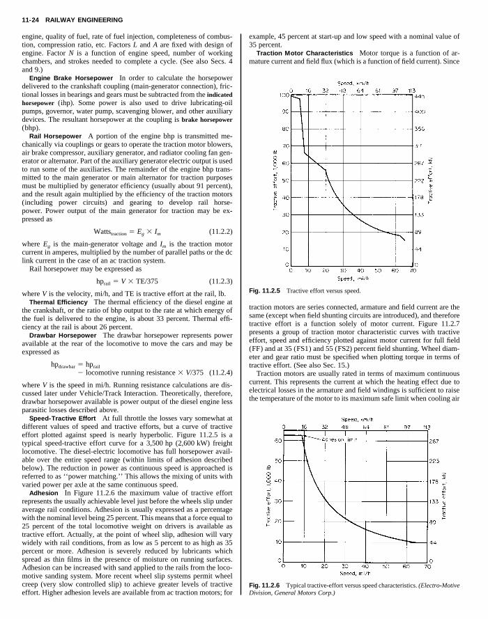
11-24 RAILWAY ENGINEERING
engine, quality of fuel, rate of fuel injection, completeness of combus-tion, compression ratio, etc. Factors L and A are fixed with design ofengine. Factor N is a function of engine speed, number of workingchambers, and strokes needed to complete a cycle. (See also Secs. 4and 9.)
Engine Brake Horsepower In order to calculate the horsepowerdelivered to the crankshaft coupling (main-generator connection), fric-tional losses in bearings and gears must be subtracted from the indicatedhorsepower (ihp). Some power is also used to drive lubricating-oilpumps, governor, water pump, scavenging blower, and other auxiliary
example, 45 percent at start-up and low speed with a nominal value of35 percent.
Traction Motor Characteristics Motor torque is a function of ar-mature current and field flux (which is a function of field current). Since
Copyright (C) 1999 by The McGraw-Hill Companies, Inc. All rights reserved. Use ofthis product is subject to the terms of its License Agreement. Click here to view.
devices. The resultant horsepower at the coupling is brake horsepower(bhp).
Rail Horsepower A portion of the engine bhp is transmitted me-chanically via couplings or gears to operate the traction motor blowers,air brake compressor, auxiliary generator, and radiator cooling fan gen-erator or alternator. Part of the auxiliary generator electric output is usedto run some of the auxiliaries. The remainder of the engine bhp trans-mitted to the main generator or main alternator for traction purposesmust be multiplied by generator efficiency (usually about 91 percent),and the result again multiplied by the efficiency of the traction motors(including power circuits) and gearing to develop rail horse-power. Power output of the main generator for traction may be ex-pressed as
Wattstraction 5 Eg 3 Im (11.2.2)
where Eg is the main-generator voltage and Im is the traction motorcurrent in amperes, multiplied by the number of parallel paths or the dclink current in the case of an ac traction system.
Rail horsepower may be expressed as
hprail 5 V 3 TE/375 (11.2.3)
where V is the velocity, mi/h, and TE is tractive effort at the rail, lb.Thermal Efficiency The thermal efficiency of the diesel engine at
the crankshaft, or the ratio of bhp output to the rate at which energy ofthe fuel is delivered to the engine, is about 33 percent. Thermal effi-ciency at the rail is about 26 percent.
Drawbar Horsepower The drawbar horsepower represents poweravailable at the rear of the locomotive to move the cars and may beexpressed as
hpdrawbar 5 hprail
2 locomotive running resistance 3 V/375 (11.2.4)
where V is the speed in mi/h. Running resistance calculations are dis-cussed later under Vehicle/Track Interaction. Theoretically, therefore,drawbar horsepower available is power output of the diesel engine lessparasitic losses described above.
Speed-Tractive Effort At full throttle the losses vary somewhat atdifferent values of speed and tractive efforts, but a curve of tractiveeffort plotted against speed is nearly hyperbolic. Figure 11.2.5 is atypical speed-tractive effort curve for a 3,500 hp (2,600 kW) freightlocomotive. The diesel-electric locomotive has full horsepower avail-able over the entire speed range (within limits of adhesion describedbelow). The reduction in power as continuous speed is approached isreferred to as ‘‘power matching.’’ This allows the mixing of units withvaried power per axle at the same continuous speed.
Adhesion In Figure 11.2.6 the maximum value of tractive effortrepresents the usually achievable level just before the wheels slip underaverage rail conditions. Adhesion is usually expressed as a percentagewith the nominal level being 25 percent. This means that a force equal to25 percent of the total locomotive weight on drivers is available astractive effort. Actually, at the point of wheel slip, adhesion will varywidely with rail conditions, from as low as 5 percent to as high as 35percent or more. Adhesion is severely reduced by lubricants whichspread as thin films in the presence of moisture on running surfaces.Adhesion can be increased with sand applied to the rails from the loco-motive sanding system. More recent wheel slip systems permit wheelcreep (very slow controlled slip) to achieve greater levels of tractiveeffort. Higher adhesion levels are available from ac traction motors; for
Fig. 11.2.5 Tractive effort versus speed.
traction motors are series connected, armature and field current are thesame (except when field shunting circuits are introduced), and thereforetractive effort is a function solely of motor current. Figure 11.2.7presents a group of traction motor characteristic curves with tractiveeffort, speed and efficiency plotted against motor current for full field(FF) and at 35 (FS1) and 55 (FS2) percent field shunting. Wheel diam-eter and gear ratio must be specified when plotting torque in terms oftractive effort. (See also Sec. 15.)
Traction motors are usually rated in terms of maximum continuouscurrent. This represents the current at which the heating effect due toelectrical losses in the armature and field windings is sufficient to raisethe temperature of the motor to its maximum safe limit when cooling air
Fig. 11.2.6 Typical tractive-effort versus speed characteristics. (Electro-MotiveDivision, General Motors Corp.)

ELECTRIC LOCOMOTIVES 11-25
Table 11.2.2 Standard Dimensions and ContactIdentification of 27-Point Control Plug and Receptaclefor Diesel-Electric Locomotives
Receptacle Wire size,point Function Code AWG
1 Power reduction setup,if used
(PRS) 14
2 Alarm signal SG 143 Engine speed DV 144* Negative N 14 or 10
Copyright (C) 1999 by The McGraw-Hill Companies, Inc. All rights reserved. Use ofthis product is subject to the terms of its License Agreement. Click here to view.
Fig. 11.2.7 Traction-motor characteristics. (Electro-Motive Division, GeneralMotors Corp.)
at maximum expected ambient temperature is forced through it at theprescribed rate by the blowers. Continuous operation at this currentlevel ideally allows the motor to operate at its maximum safe powerlevel, with waste heat generated equal to heat dissipated. The tractiveeffort corresponding to this current is usually somewhat lower than thatallowed by adhesion at very low speeds. Higher current values may bepermitted for short periods of time (as when starting). These ratings arespecified in time intervals and are posted on or near the load meter(ammeter) dial in the cab.
Maximum Speed Traction motors are also rated in terms of theirmaximum safe speed in r/min, which in turn limits locomotive speed.The gear ratio and wheel diameter are directly related to speed as well asthe maximum tractive effort and the minimum speed at which fullhorsepower can be developed at the continuous rating of the motors.Maximum locomotive speed may be expressed as follows:
(mi/h)max 5wheel diameter (in) 3 maximum motor r/min
gear ratio 3 336(11.2.5)
where the gear ratio is the number of teeth on the motor gear mountedon the axle divided by the number of teeth on the pinion mounted on thearmature shaft.
Locomotive Compatibility The AAR has developed two standardsin an effort to improve compatibility between locomotives of differentmodel, manufacture, and ownership: a standard 27-point control system(Standard S-512, Table 11.2.2) and a standard control stand (StandardS-523, Fig. 11.2.8). These features allow locomotives to be combined inmultiple-unit service on all railroads irrespective of model or manufac-turer.
Energy Conservation Efforts to improve efficiency and fuel econ-omy have resulted in major changes in the prime movers, includingmore efficient turbocharging, fuel injection, and combustion. The aux-iliary (parasitic) power demands have also been reduced with improve-ments which include fans and blowers which only move the air requiredby the immediate demand, air compressors that declutch when un-loaded, and a selective low-speed idle. Fuel-saver switches permitdropping trailing locomotive units off the line when less than maximumpower is required, and allow the remaining units to operate at maximumefficiency.
ELECTRIC LOCOMOTIVES
Electric locomotives are presently in limited use in North America.Freight locomotives are in dedicated service primarily for coal or min-
5 Emergency sanding ES 146 Generator field GF 127 Engine speed CV 148 Forward FO 129 Reverse RE 12
10 Wheel slip WS 1411 Spare 1412 Engine speed BV 1413 Positive control PC 1214 Spare 1415 Engine speed AV 1416 Engine run ER 1417 Dynamic brake B 1418 Unit selector circuit US 1219 2d negative, if used (NN) 1220 Brake warning light BW 1421 Dynamic brake BG 1422 Compressor CC 1423 Sanding SA 1424 Brake control /power
reduction controlBC/PRC 14
25 Headlight HL 1226 Separator blowdown/
remote resetSV/RR 14
27 Boiler shutdown BS 14
* Receptacle point 4—AWG wire size 12 is ‘‘standard’’ and AWG wire size 10 is‘‘Alternate standard’’ at customer’s request. A dab of white paint in the cover latch cavitymust be added for ready identification of a no. 10 wire present in a no. 4 cavity.
eral hauling. Electric passenger locomotives are used in high-densityservice in the northeastern United States and a combination electricpassenger and freight locomotive has been produced for use in Mexico.
Electric locomotives draw power from overhead catenary systems.While earlier systems used either direct current up to 3,000 V or single-phase alternating current at 11,000 V, 25 Hz, the newer systems use25,000 or 50,000 V at 60 Hz. The higher voltage levels can only be usedwhere clearances permit. Three-phase supply was tried briefly in thiscountry and overseas about 50 years ago, but was abandoned because ofthe complexity of the required double catenary.
While the older dc locomotives used resistance control, ac locomo-tives have used a variety of systems including Scott-connected trans-formers; series ac motors; motor generators and dc motors; ignitronsand dc motors; silicon thyristors and dc motors; and, more recently,chopper control in experimental locomotives. Examples of the variouselectric locomotives in service are shown in Table 11.2.1.
An electric locomotive used in high-speed passenger service is shownin Fig. 11.2.9. High short-time ratings (Figs. 11.2.10 and 11.2.11)render electric locomotives suitable for passenger service where highacceleration rates and high speeds are combined to meet demandingschedules.
The modern electric locomotive in Fig. 11.2.9 obtains power for themain circuit and motor control from the catenary through a pantograph.A motor-operated switch provides for the transformer change fromseries to parallel connection of the primary windings to give a constantsecondary voltage with either 25 kV or 12.5 kV primary supply. Theconverters for armature current consist of two asymmetric type bridgesfor each motor. The traction-motor fields are each separately fed from aone-way connected-field converter.
Identical control modules separate the control of motors on eachtruck. Motor sets are therefore connected to the same transformer wind-

11-26 RAILWAY ENGINEERING
Fig. 11.2.8 AAR standard control stand.
ing. Wheel slip correction is also modularized, utilizing one modulefor each two-motor truck set. This correction is made with a comple-mentary wheel-slip detection and correction system. A magneticpickup speed signal is used for the basic wheel slip. Correction is en-hanced by a magnetoelastic transducer used to measure force swings inthe traction-motor reaction rods. This system provides the final limitcorrection.
To optimize the utilization of available adhesion, the wheel-slip con-trol modules operate independently to allow the motor modules to re-ceive different current references depending on their respective adhe-
All auxiliary machines, air compressor, traction motor blower, cool-ing fans, etc., are driven by three-phase 400-V, 60-Hz induction motorspowered by a static inverter which has a rating of 175 kVA at a 0.8power factor. When cooling requirements are reduced, the control sys-tem automatically reduces the voltage and frequency supplied to theblower motors to the required level. As a backup, the system can bepowered by the static converter used for the head-end power require-ments of the passenger cars. This converter has a 500-kW, 480-V,three-phase, 60-Hz output capacity and has a built-in overload capacityof 10 percent for half of any 1-h period.
Copyright (C) 1999 by The McGraw-Hill Companies, Inc. All rights reserved. Use ofthis product is subject to the terms of its License Agreement. Click here to view.
sion conditions.
Fig. 11.2.9 Locomotive general arrangement. (Courtesy of M. Ephrai
Dynamic brake resistors are roof-mounted and are cooled by ambient
m, ASME, Rail Transportation Division.)

FREIGHT CARS 11-27
airflow induced by locomotive motion. The dynamic brake capacityrelative to train speed is shown in Fig. 11.2.12.
Many electric locomotives utilize traction motors identical to thoseused on diesel-electric locomotives. Some, however, use frame sus-
pended motors with quill-drive systems (Fig. 11.2.13). In these systems,torque is transmitted from the traction motor by a splined coupling to aquill shaft and rubber coupling to the gear unit. This transmission allowsfor greater relative movement between the traction motor (truck frame)and gear (wheel axle) and reduces unsprung weight.
Copyright (C) 1999 by The McGraw-Hill Companies, Inc. All rights reserved. Use ofthis product is subject to the terms of its License Agreement. Click here to view.
Fig. 11.2.10 Speed-horsepower characteristics (half-worn wheels). [Gearratio 5 85/36; wheel diameter 5 50 in (1,270 mm); ambient temperature 5 60°F(15.5°C).] (Courtesy of M. Ephraim, ASME, Rail Transportation Division.)
Fig. 11.2.11 Tractive effort versus speed (half-worn wheels). [Voltage 511.0 kV at 25 Hz; gear ratio 5 85/36; wheel diameter 5 50 in (1,270 mm).](Courtesy of M. Ephraim, ASME, Rail Transportation Division.)
Fig. 11.2.12 Dynamic-brake performance. (Courtesy of M. Ephraim, ASME,Rail Transportation Division.)
Fig. 11.2.13 Frame-suspended locomotive transmission. (Courtesy of M.Ephraim, ASME, Rail Transportation Division.)
FREIGHT CARS
Freight Car Types
Freight cars are designed and constructed for either general service orspecific ladings. The Association of American Railroads (AAR) hasestablished design and maintenance criteria to assure the interchange-ability of freight cars on all North American railroads. Freight carswhich do not conform to AAR standards have been placed in service byspecial agreement of the railroads over which the cars operate. TheAAR ‘‘Manual of Standards and Recommended Practices’’ specifiesdimensional limits, weights, and other design criteria for cars whichmay be freely interchanged between North American railroads. Thismanual is revised annually by the AAR. Many of the standards arereproduced in the ‘‘Car and Locomotive Cyclopedia,’’ which is revisedabout every 4 years. Safety appliances (such as end ladders, sill steps,and uncoupling levers), braking equipment, and certain car design fea-tures and maintenance practices must comply with the Safety Appli-ances Act, the Power Brake Law, and the Freight Car Safety Standardscovered by the Federal Railroad Administration’s (FRA) Code of Fed-eral Regulations (CFR Title 49). Maintenance practices are discussed inthe Field Manual of the AAR Interchange Rules and pricing informationis provided in the companion Office Manual.
The AAR identifies most cars by nominal capacity, type, and in somecases there are restrictions as to type of load (i.e., food, automobileparts, coil steel, etc.). Most modern cars have nominal capacities ofeither 70 or 100 tons.* A 100-ton car is limited to a maximum gross railload of 263,000 lb (119.3 t*) with 61⁄2 by 12 in (165 by 305 mm) axlejournals, four pairs of 36-in (915-mm) wheels and a 70-in (1,778 mm)rigid wheel base. Some 100-ton cars are rated at 286,000 lb and arehandled by individual railroads on specific routes or by mutual agree-ment between the handing railroads. A 70-ton car is limited to a maxi-mum gross rail load of 220,000 lb (99.8 t) with 6 by 11 in (152 by280 mm) axle journals, four pairs of 33-in (838-mm) wheels with truckshaving a 66-in (1,676-mm) rigid wheel base.
On some special cars where height limitations are critical, 28-in(711-mm) wheels are used with 70-ton axles and bearings. In thesecases wheel loads are restricted to 22,400 lb (10.2 t). Some special carsare equipped with 38-in (965-mm) wheels in four wheel trucks having 7by 14 in (178 by 356 mm) axle journals and 72-in (1,829-mm) wheelbase. This application is prevelant in articulated double-stack (two-high) container cars. Interchange of these very heavy cars is by mutualagreement between the operating railroads involved.
* 1 ton 5 1 short ton 5 2,000 lb; 1 t 5 1 metric ton 5 1,000 kg 5 2205 lb.

11-28 RAILWAY ENGINEERING
The following are the most common car types in service in NorthAmerica. Dimensions given are for typical cars; actual measurementsmay vary.
Box Cars (Fig. 11.2.14a) There are six popular box-car types.1. Unequipped box cars may have sliding doors or plug doors. Plug
doors provide a tight seal from weather and a smooth interior. Un-equipped box cars are usually of 70-ton capacity. These cars havetongue-and-groove or plywood lining on the interior sides and ends withnailable floors (either wood or steel with special grooves for lockingnails). The cars carry typical general merchandise lading: packaged,
High-side gondola cars (Fig. 11.2.14d) are open-top cars typically usedto haul coal or wood chips. These cars are similar to open-top hoppercars in volume but require a rotary coupler on one end for rotary dump-ing to discharge lading since they do not have bottom outlets. Rotary-dump coal gondolas are usually used in dedicated, unit-train servicebetween a coal mine and an electric power plant. The length overcoupler pulling faces is approximately 53 ft 1 in (16.2 m) to suit thestandard coal dumper. [100 ton: L 5 50 ft 51⁄2 in (15.4 m), H 5 11 ft9 in (3.6 m), W 5 10 ft 53⁄8 in (3.2 m), truck centers 5 50 ft 4 in(15.3 m).] Wood chip cars are used to haul chips from sawmills to paper
Copyright (C) 1999 by The McGraw-Hill Companies, Inc. All rights reserved. Use ofthis product is subject to the terms of its License Agreement. Click here to view.
canned, or bottled foodstuffs; finished lumber; bagged or boxed bulkcommodities; or, when equipped with temporary door fillers, bulk com-modities such as grain. [70 ton: L 5 50 ft 6 in (15.4 m), H 5 11 ft 0 in(3.4 m), W 5 9 ft 6 in (2.9 m), truck centers 5 40 ft 10 in (12.4 m).]
2. Specially equipped box cars usually have the same dimensions asunequipped cars but include special equipment to restrain lading fromimpacts and over-the-road vibrations. Equipped cars may have hydrau-lic-cushion units to dampen longitudinal shock at the couplers.
3. Insulated box cars have plug doors and special insulation. Thesecars carry foodstuffs such as unpasteurized beer, produce, and dairyproducts. These cars may be precooled by the shipper and maintain aheat loss rate equivalent to 1°F (0.55°C) per day.
4. Refrigerated box cars are used where transit times are longer.These cars are equipped with diesel-powered refrigeration units and areprimarily used to carry produce. These are often 100-ton cars [L 5 52 ft6 in (16.0 m), H 5 10 ft 6 in (3.2 m), truck centers 5 42 ft 11 in(13.1 m)].
5. ‘‘All door’’ box cars have doors which open the full length of thecar for loading package lumber products such as plywood and gypsumboard.
6. High-cubic-capacity box cars with an inside volume of 10,000 ft3
(283 m3) have been designed for light-density lading.Box-car door widths vary from 6 to 10 ft for single-door cars and 16
to 20 ft (4.9 to 6.1 m) for double-door cars. ‘‘All door’’ cars have cleardoorway openings in excess of 25 ft (7.6 m). The floor height above railfor an empty uninsulated box car is approximately 44 in (1,120 mm)and for an empty insulated box car approximately 48 in (1,220 mm).The floor height of a loaded car can be as much as 3 in (76 mm) lowerthan the empty car.
Covered hopper cars (Fig. 11.2.14b) are used to haul bulk commodi-ties which must be protected from the environment. Modern coveredhopper cars are typically 100-ton cars with roof hatches for loading andfrom two to six bottom outlets for discharge. Cars used for dense com-modities, such as fertilizer or cement, have two bottom outlets, roundroof hatches, and volumes of 3,000 to 4,000 ft3 (84.9 to 113.2 m3). [100ton: L 5 39 ft 3 in (12.0 m). H 5 14 ft 10 in (4.5 m), truck centers 526 ft 2 in (8.0 m).] Cars used for grain service (corn, wheat, rye, etc.)have three or four bottom outlets, longitudinal trough roof hatches, andvolumes of from 4,000 to 5,000 ft3 (113 to 142 m3). Cars used forhauling plastic pellets have four to six bottom outlets (for pneumaticunloading with a vacuum system), round roof hatches, and volumes offrom 5,000 to 6,000 ft3 (142 to 170 m3). [100 ton: L 5 65 ft 7 in(20.0 m), H 5 15 ft 5 in (4.7 m), truck centers 5 54 ft 0 in (16.5 m).]
Open-top hopper cars (Fig. 11.2.14c) are used for hauling bulk com-modities such as coal, ore, or wood chips. A typical 100-ton coal hoppercar will vary in volume depending on the light weight of the car anddensity of the coal to be hauled. Volumes range from 3,900 to 4,800 ft3
(110 to 136 m3). Cars may have three or four manually operated or 12 to16 automatically operated bottom hoppers. Some cars are equipped withrotating couplers on one end to allow rotary dumping without uncou-pling. [100 ton: L 5 53 ft 1⁄2 in (16.2 m), H 5 12 ft 81⁄2 in (3.9 m), truckcenters 5 40 ft 6 in (12.3 m).] Cars intended for aggregate or ore ser-vice have smaller volumes for the more dense commodity. These carstypically have two manual bottom outlets. [100 ton: L 5 40 ft 8 in(12.4 m), H 5 11 ft 107⁄8 in (3.6 m), truck centers 5 29 ft 9 in (9.1 m).]Hopper cars used for chip services are configured for low-density loads.Volumes range from 6,500 to 7,500 ft3 (184 to 212 m3).
mills or particle-board manufacturers. These high-volume cars are ei-ther rotary-dumped or, when equipped with end doors, end-dumped.[100 ton: L 5 62 ft 3 in (19.0 m), H 5 12 ft 7 in (3.8 m), W 5 10 ft53⁄8 in (3.2 m), truck centers 5 50 ft 4 in (15.3 m).] Rotary-dump ag-gregate or ore cars, called ‘‘ore jennies,’’ have smaller volumes for thehigh-density load.
Bulkhead flat cars (Fig. 11.2.14e) are used for hauling such commodi-ties as packaged finished lumber, pipe, or with special inward cantedfloors, pulpwood. Both 70- and 100-ton bulkhead flats are used. Typicaldeck heights are approximately 50 in (1,270 mm). [100 ton: L 5 61 ft3⁄4 in (18.6 m), W 5 10 ft 1 in (3.1 m), H 5 11 ft 0 in (3.4 m), truckcenters 5 55 ft 0 in (16.8 m).] A few special bulkhead flat cars de-signed for pulpwood and lumber service have a full-height, longitudinaldivider from bulkhead to bulkhead.
Tank cars (Fig 11.2.14f ) are used for liquids, compressed gases, andother ladings, such as sulfur, which can be loaded and unloaded in amolten state. Nonhazardous liquids such as corn syrup, crude oil, andmineral spring water are carried in nonpressure cars. Cars used to haulhazardous substances such as liquefied petroleum gas (LPG), vinylchloride, and anhydrous ammonia are regulated by the U.S. Departmentof Transportation. Newer and earlier-built retrofitted cars equipped forhazardous commodities have safety features including safety valves,specially designed top and bottom ‘‘shelf’’ couplers which increase theinterlocking effect between couplers and decrease the danger of disen-gagement due to derailment, head shields on the ends of the tank toprevent puncturing, bottom-outlet protection if bottom outlets are used,and thermal insulation to reduce the risk of rupturing in a fire. Thesefeatures resulted from industry-government studies in the RPI-AARTank Car Safety Research and Test Program.
Cars for sulfur and other viscous-liquid service have heating coils onthe shell so that steam may be used to liquefy the lading for discharge.[Pressure cars, 100 ton: volume 5 20,000 gal (75.7 m3), L 5 59 ft113⁄4 in (18.3 m), truck centers 5 49 ft 01⁄4 in (14.9 m).] [Nonpressure,100 ton, volume 5 21,000 gal (79.5 m3), L 5 51 ft 31⁄4 in (15.6 m),truck centers 5 38 ft 111⁄4 in (11.9 m).]
Intermodal Cars Conventional 89-ft (27.1-m) intermodal flat carsare equipped to haul one 45-ft (13.7 m) and one 40-ft (12.2 m) trailerwith or without nose-mounted refrigeration units, two 45-ft (13.7 m)trailers (dry vans), or combinations of containers from 20 to 40 ft (6.1 to12.2 m) in length. Hitches to support trailer fifth wheels may be fixedfor trailer-only cars or retractable for conversion to haul containers orfor driving trailers onto the cars where circus loading is required. Trailerhauling service (Fig. 11.2.14g) is called TOFC (trailer on flat car).Container service (Fig. 11.2.14h) is called COFC (container on flat car).[70 ton: L 5 89 ft 4 in (27.1 m), W 5 10 ft 3 in (3.1 m), truck centers 564 ft 0 in (19.5 m).]
Introduction of larger trailers in highway service has led to the devel-opment of alternative TOFC and COFC cars. One technique involvesarticulation of skeletonized or well-type units into multiunit cars forlift-on loading and lift-off unloading (stand-alone well car, Fig.11.2.14n and articulated well car, Fig. 11.2.14o). These cars are typi-cally composed of from three to ten units. Well cars consist of a centerwell for double-stacked containers. [10-unit, skeletonized car; L 5 46 ft63⁄8 in (14.2 m) per end unit, L 5 465 ft 31⁄2 in (141.8 m).]
Another approach to hauling larger trailers is the two-axle skeleton-ized car. These cars, used either singly or in multiple combinations, canhaul a single trailer from 40 to 48 ft long (12.2 to 14.6 m) with nose-

FREIGHT CARS 11-29
(a) Box car
(c) Open top hopper car
(e) Bulkhead flat car
(g) Trailers on flat car
(i) Multilevel auto rack car
(k) General-purpose flat car
(m) Schnabel car
(o) Articulated double-stack car
(b) Covered hopper car
(d) High side gondola car
(f) Tank car
(h) Containers on flat car
(j) Mill gondola car
(l) Depressed-center flat car
(n) Stand-alone well car
Fig. 11.2.14 Typical freight cars.
mounted refrigeration unit and 36- or 42-in (914- to 1070-mm) spacingbetween the kingpin and the front of the trailer.
Bilevel and trilevel auto rack cars (Fig. 11.2.14i) are used to haulfinished automobiles and other vehicles. Most recent designs of thesecars feature fully enclosed racks to provide security against theft andvandalism. [70 ton: L 5 89 ft 4 in (27.2 m), H 5 18 ft 11 in (5.8 m),W 5 10 ft 7 in (3.2 m), truck centers 5 64 ft 0 in (19.5 m).]
Mill gondolas (Fig. 11.2.14j) are 70-ton or 100-ton open-top cars prin-cipally used to haul pipe, structural steel, scrap metal, and when spe-cially equipped, coils of aluminum or tinplate and other steel materials.
restraint dunnage. Some heavy-duty six-axle cars are used for haulingoff-highway vehicles such as army tanks and mining machinery. [100ton, four axle: L 5 60 ft 0 in (18.3 m), H 5 3 ft 9 in (1.1 m), truckcenters 5 42 ft 6 in (13.0 m).] [200 ton, 8 axle: L 5 44 ft 4 in (13.5 m),H 5 4 ft 0 in (1.2 m), truck centers 5 33 ft 9 in (10.3 m).]
Depressed-center flat cars (Fig. 11.2.14l) are used for hauling trans-formers and other heavy, large materials which require special clear-ance considerations. Depressed-center flat cars may have four-, six-, ordual four-axle trucks with span bolsters, depending on weight require-ments.
Copyright (C) 1999 by The McGraw-Hill Companies, Inc. All rights reserved. Use ofthis product is subject to the terms of its License Agreement. Click here to view.
[100 ton: L 5 52 ft 6 in (16.0 m), W 5 9 ft 6 in (2.9 m), H 5 4 ft 6 in(1.4 m), truck centers 5 43 ft 6 in (13.3 m).]
General-purpose or machinery flat cars (Fig. 11.2.14k) are 70-ton or100-ton cars used to haul machinery such as farm equipment and high-way tractors. These cars usually have wood decks for nailing lading-
Schnabel cars (Fig. 11.2.14m) are special cars for transformers andnuclear components. With these cars the load itself provides the centersection of the car structure during shipment. Some Schnabel cars areequipped with hydraulic controls to lower the load for height restric-tions and shift the load laterally for wayside restrictions. [472 ton: L 5

11-30 RAILWAY ENGINEERING
22 ft 10 in to 37 ft 10 in (7.0 to 11.5 m), truck centers 5 55 ft 6 in to70 ft 6 in (16.9 to 21.5 m).] Schnabel cars must be operated in specialtrains.
Freight Car Design
The AAR provides specifications to cover minimum requirements fordesign and construction of new freight cars. Experience has demon-strated that the AAR Specifications alone do not ensure an adequate cardesign for all service conditions. The designer must be familiar with theintended service and increase the design criteria for the particular car
pact load is 600,000 lb (2.7 MN). In all cases, the structural connectionsto the car must be capable of withstanding a static compressive(squeeze) end load of 1,000,000 lb (4.44 MN) or a dynamic (impact)compressive load of 1,250,000 lb (5.56 MN).
The AAR has recently adopted requirements for unit trains of high-utilization cars to be designed for 3,000,000 mi (4.8 Gm) of servicebased upon fatigue life estimates. General-interchange cars which accu-mulate less mileage in their life should be designed for 1,000,000 mi(1.6 Gm) of service. Road environment spectra for various locationswithin the car are being developed for different car designs for use in
Copyright (C) 1999 by The McGraw-Hill Companies, Inc. All rights reserved. Use ofthis product is subject to the terms of its License Agreement. Click here to view.
above the minimum criteria provided by the AAR. The AAR require-ments include stress calculations for the load-carrying members of thecar and physical tests which may be required at the option of the AARcommittee approving the car design. In some cases, it is advisable tooperate an instrumented prototype car in service to detect problemswhich might result from unexpected track or train-handling inputforces. The car design must comply with width and height restrictionsshown in AAR clearance plates furnished in the specifications, Fig.11.2.15. In addition, there are limitations on the height of the center of
Fig. 11.2.15 AAR plate B equipment-clearance diagram.
gravity of the loaded car and on the vertical and horizontal curvingcapability allowed by the clearance provided at the coupler. The AARprovides a method of calculating the minimum radius curve which thecar design can negotiate when coupled to another car of the same type orto a standard AAR ‘‘base’’ car. In the case of horizontal curves, therequirements are based on the length over the pulling faces of the car.
In the application for approval of a new or untried type of car, the CarConstruction Committee of the AAR may require either additional cal-culations or tests to assess the design’s ability to meet the AAR mini-mum requirements. These tests might consist of a static compressiontest of 1,000,000 lb (4.4 MN), a static vertical test applied at thecoupler, and impact tests simulating yard impact conditions.
Freight cars are designed to withstand single-ended impact or cou-pling loads based upon the type of cushioning provided in the car de-sign. Conventional friction, elastomer, or combination draft gears orshort-travel hydraulic cushion units which provide less than 6 in(152 mm) of travel require a structure capable of withstanding a1,250,000-lb (5.56-MN) impact load. For cars with hydraulic units thatprovide greater than 14 in (356 mm) of travel, the required design im-
this analysis. The fatigue strengths of various welded connections areprovided in the AAR ‘‘Manual of Standards and Recommended Prac-tices,’’ Sec. C, Part II.
Many of the design equations and procedures are available from theAAR. Important information on car design and approval testing is con-tained in the AAR ‘‘Manual of Standards and Recommended Practice,’’Sec. C-II M-1001, Chap. XI.
Freight-Car Suspension
Most freight cars are equipped with standard three-piece trucks (Fig.11.2.16) consisting of two side-frame castings and one bolster casting.Side-frame and bolster designs are subjected to both static and fatiguetest requirements specified by the AAR. The bolster casting is equippedwith a female centerplate bowl upon which the car body rests and sidebearings located [generally 25 in (635 mm)] each side of the centerline.
Fig. 11.2.16 Unit-beam roller-bearing truck with inset showing plain-bearingjournal. (AAR Research and Test Department.)

FREIGHT CARS 11-31
In most cases, the side bearings have clearance to the car body and areequipped with either flat sliding plates or rollers. In some cases, con-stant-contact side bearings or centerplate extension pads provide a resil-ient material between the car body and the truck bolster.
The centerplate arrangement consists of various styles of wear platesor friction materials and a vertical loose or locked pin between the truckcenterplate and the car body.
Truck springs nested into the bottom of the side-frame opening sup-port the end of the truck bolster. Requirements for spring designs and
Table 11.2.3 Wheel and Journal Sizes of Eight-Wheel Cars
Nominal car Journal Wheelcapacity, Maximum gross (bearing) diameter,
ton weight, lb size, in in
50 177,000 51⁄2 3 10 33* 179,200 6 3 11 28
70 220,000 6 3 11 33100 263,000‡ 61⁄2 3 12 36125† 315,000 7 3 12 38
Copyright (C) 1999 by The McGraw-Hill Companies, Inc. All rights reserved. Use ofthis product is subject to the terms of its License Agreement. Click here to view.
the grouping of springs are generally specified by the AAR. Histori-cally, the damping provided within the spring group has utilized a com-bination of springs and friction wedges. In addition to friction wedges,in more recent years, some cars have been equipped with hydraulicdamping devices which parallel the spring group.
A few trucks with a ‘‘steering’’ feature which includes an intercon-nection between axles to increase the lateral interaxle stiffness and de-crease the interaxle yaw stiffness. Increased lateral stiffness improvesthe lateral stability and decreased yaw stiffness improves the curvingcharacteristics.
Freight-Car Wheel-Set Design
A freight-car wheel set consists of wheels, axle, and bearings. Cast- andwrought-steel wheels are used on freight cars in North America (AAR‘‘Manual of Standards and Recommended Practice,’’ Sec. G). Freight-car wheels are subjected to thermal loads from braking, as well asmechanical loads at the wheel-rail interface. Experience with thermaldamage to wheels has led to the introduction of ‘‘low stress’’ or curvedplate wheels (Fig. 11.2.17). These wheels are less susceptible to the
Fig. 11.2.17 Wheel-plate designs. (a) Flat plate; (b) parabolic plate; (c) S-curved plate.
development of circumferential tensile residual stresses which renderthe wheel vulnerable to sudden failure if a flange or rim crack occurs.New wheel designs introduced for interchange service must be evalu-ated using a finite-element technique employing both thermal and me-chanical loads (AAR S-660).
Freight-car wheels range in diameter from 28 to 38 in (711 to965 mm) depending on car weight, Table 11.2.3. The old AAR standardtread profile (Fig. 11.2.18a) has been replaced with the AAR-1B (Fig.11.2.18c) profile which represents a worn profile to minimize earlytread loss due to wear and provides a stable profile over the life of thetread. Several variant wheel tread profiles, including the AAR-1B, weredeveloped from the basic Heumann design, Fig. 11.2.18b. One of thesewas for application in Canada and provided increasing conicity into the
Fig. 11.2.18 Wheel-tread designs. (a) Obsolete st
* Limited by wheel rating.† Not approved for free interchange.‡ 286,000 in special cases.
throat of the flange, a design feature of the Heumann profile. Thisreduces curving resistance and increases wheel wear life.
Wheels are also specified by chemistry and heat treatment. Low-stress wheel designs of Classes B and C are required for freight cars.Class B wheels have a carbon content of 0.57 to 0.67 percent and arerim-quenched. Class C wheels have a carbon content of 0.67 to 0.77percent and are also rim-quenched. Rim quenching provides a hardenedrunning surface for a long wear life. Lower carbon levels than those inClass B may be used where thermal cracking is experienced but freight-car equipment generally does not require their use.
Axles used in interchange service are solid steel forgings with raisedwheel seats. Axles are specified by journal size for different car capaci-ties, Table 11.2.3.
Most freight car bearings are grease-lubricated, tapered-roller bear-ings (see Sec. 8). The latest bearing designs eliminate the need forperiodic field lubrication.
Wheels are mounted and secured on axles with an interference fit.Bearings are mounted with an interference fit and retained by an end capbolted to the end of the axle. Wheels and bearings for cars in inter-change service must be mounted by an AAR-inspected and -approvedfacility.
Special Features
Many components are available to enhance the usefulness of freightcars. In most cases, the design or performance of the component isspecified by the AAR.
Coupler Cushioning Switching of cars in a classification yard canresult in relatively high coupler forces at the time of the impact betweenthe moving and standing cars. Nominal coupling speeds of 4 mi/h (6.4km/h) or less are sometimes exceeded, with lading damage a possibleresult. Conventional cars are equipped with an AAR-approved draftgear, usually a friction-spring energy-absorbing device, mounted be-tween the coupler and the car body. The rated capacity of draft gearsranges between 20,000 ft ? lb (27.1 kJ) for earlier units to over 65,000ft ? lb (88.1 kJ) for later designs. Impact forces of 1,250,000 lb(5.56 MN) can be expected when a moving 100-ton car strikes a stringof standing cars at 8 to 10 mi/h (12.8 to 16 km/h). Hydraulic cushioningdevices are available which will reduce the impact force to 500,000 lb(2.22 MN) at impact speeds of 12 to 14 mi/h (19 to 22 km/h). These
andard AAR; (b) Heumann, (c) new AAR-1B.

11-32 RAILWAY ENGINEERING
devices may be either mounted at each end of the car (end-of-car de-vices) or mounted in a long beam which extends from coupler to coupler(sliding centersill devices).
Lading Restraint Many forms of lading restraint are available, fromtie-down chains for automobiles on rack cars to movable bulkheads forboxcars. Most load-restraining devices are specified by the AAR‘‘Manual of Standards and Recommended Practices’’ and approved carloading arrangements are specified in AAR ‘‘Loading Rules,’’ a multi-volume publication for enclosed, open-top, and TOFC and COFC cars.
Covered Hopper Car Discharge Gates The majority of covered
ke
same time connects the brake cylinders to exhaust. Brake pipe pressureis reduced when the engineer’s brake valve is placed in a service posi-tion, and the control valve cuts off the charging function and allows thereservoir air on each car to flow into the brake cylinder. This moves thepiston and, through a system of levers and rods, pushes the brake shoesagainst the wheel treads.
When the engineer’s automatic brake valve is placed in the emer-gency position the brake pipe pressure (BP) is reduced very rapidly. Thecontrol valves on each car move to the emergency-application positionand rapidly open a large vent valve, exhausting brake pipe pressure to
Copyright (C) 1999 by The McGraw-Hill Companies, Inc. All rights reserved. Use ofthis product is subject to the terms of its License Agreement. Click here to view.
hopper cars are equipped with rack-and-pinion slide gates which allowthe lading to discharge by gravity onto conveyor equipment locatedbetween the rails. These gates can be operated manually with a simplebar or a torque-multiplying wrench or mechanically with an impact orhydraulic wrench. Many special covered hopper cars are equipped withdischarge gates with nozzles and metering devices for vacuum or pneu-matic unloading.
Coupling Systems A majority of freight cars are connected withAAR standard couplers. A specification has been developed to permitthe use of alternative coupling systems such as articulated connectors,drawbars, and rotary-dump couplers.
Freight-Train Braking
The retarding forces acting on a railway train are rolling and mechanicalresistance, aerodynamic drag, curvature and grade, plus that force re-sulting from the friction of the brake shoes rubbing on the wheel treads.On locomotives so equipped, the dynamic or rheostatic brake using thetraction motors as generators can provide all or a portion of the retardingforce to control train speed on down grades and sometimes during retar-dation and service stops.
Quick-action automatic air brakes of the type specified by the AARare the common standard in North America. With the automatic airbrake, the brake pipe extends through every vehicle in the train, con-nected by hoses between each locomotive unit and car. The front andrear brake pipe angle cocks are closed.
Air pressure is provided by compressors on the locomotive units tothe main reservoirs, usually at 130 to 150 lb/in2 (900 to 965 kPa).(Pressure values are gage pressures.) The engineer’s automatic brakevalve in release position provides air to the brake pipe on freight trainsat reduced pressure, usually at 75, 80, 85, or 90 lb/in2 (520, 550, 585, or620 kPa) depending on the type of service, train weight, descendinggrades, and speeds that a train will operate. In passenger service, brakepipe pressure is usually 90 or 100 lb/in2 (620 or 760 kPa).
When brake pipe pressure is increased, the control valve allows thereservoir capacity on each car and locomotive to be charged and at the
Table 11.2.4 Braking Ratios, AAR Standard S-401
Type of brake rigging and shoes
Conventional body-mounted brake rigging or truck-mounted bra
rigging using levers to transmit brake cylinder force to thebrake shoesCars equipped with cast iron brake shoesCars equipped with high-friction composition brake shoes
Direct-acting brake cylinders not using levers to transmit brakecylinder force to the brake shoes
Cars equipped with cast iron brake shoesCars equipped with high-friction composition brake shoes
Cabooses†Cabooses equipped with cast iron brake shoesCabooses equipped with high-friction composition brake shoes
* Hand brake force applied at the horizontal hand brake chain with AAR ce† Effective for cabooses ordered new after July 1, 1982, hand brake ratios fNOTE: Above braking ratios also apply to cars equipped with empty and loa
With 50 lb/in2 brakecylinder pressure
Percent of grossrail load
Min. Max.
Maximumpercent of
light weight
Hand brake*
Minimumpercent ofgross rail
load
atmosphere. This will serially propagate the emergency applicationthrough the train at from 900 to 950 ft/s (280 to 290 m/s). With thecontrol valve in the emergency position both auxiliary- and emergency-reservoir volumes (pressures) equalize with the brake cylinder, andhigher brake cylinder pressure (BCP) results, building up at a faster ratethan in service applications.
The foregoing briefly describes the functions of the fundamental au-tomatic air brake based on the functions of the control valve. AAR-ap-proved brake equipment is required on all freight cars used in inter-change service. The functions of the control valve have been refined topermit the handling of longer trains by more uniform brake perfor-mance. Important improvements in this design have been (1) reductionof the time required to apply the brakes on the last car of a train, (2)more uniform and faster release of the brakes, and (3) availability ofemergency application with brake pipe pressure greater than 40 lb/in2
(275 kPa).The braking ratio of a car is defined as the ratio of brake shoe (nor-
mal) force to the car’s rated gross weight. Two types of brake shoes,high-friction composition and high-phosphorus cast iron, are in use ininterchange service. As these shoes have very different friction charac-teristics, different braking ratios are required to assure uniform trainbraking performance (Table 11.2.4). Actual or net shoe forces are mea-sured with calibrated devices. The calculated braking ratio R (nominal)is determined from the equation
R 5 PLANE 3 100/W (11.2.6)
where P 5 brake cylinder pressure, 50 lb/in2 gage; L 5 mechanical ratioof brake levers; A 5 brake cylinder area, in2; N 5 number of brakecylinders; E 5 brake rigging efficiency 5 Er 3 Eb 3 Ec ; and W 5 carweight (lb).
To estimate rigging efficiency consider each pinned joint and hori-zontal sliding joint as a 0.01 loss of efficiency; i.e., in a system with 20pinned and horizontal sliding joints, Er 5 0.80. For unit-type (hanger-less) brake beams Eb 5 0.90 and for the brake cylinder Ec 5 0.95,giving overall efficiency of 0.684 or 68.4 percent.
13 20 53 136.5 10 30 11
6.5 10 33 11
35–4518–23
rtified or AAR approved hand brake.or cabooses to the same as lightweight ratios for cabooses.d brake equipment.
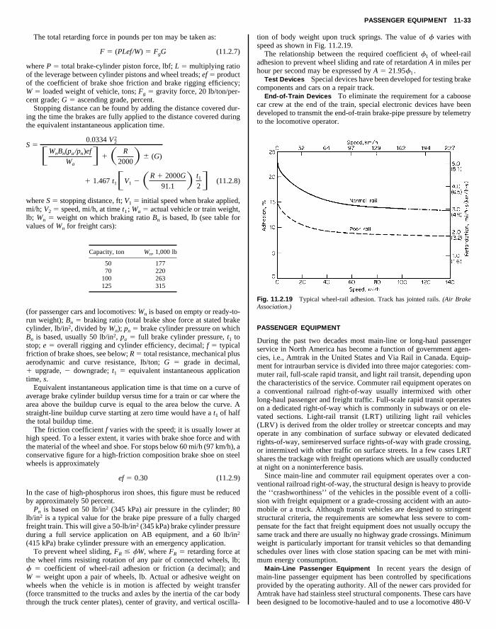
PASSENGER EQUIPMENT 11-33
The total retarding force in pounds per ton may be taken as:
F 5 (PLef/W) 5 FgG (11.2.7)
where P 5 total brake-cylinder piston force, lbf; L 5 multiplying ratioof the leverage between cylinder pistons and wheel treads; ef 5 productof the coefficient of brake shoe friction and brake rigging efficiency;W 5 loaded weight of vehicle, tons; Fg 5 gravity force, 20 lb/ton/per-cent grade; G 5 ascending grade, percent.
Stopping distance can be found by adding the distance covered dur-ing the time the brakes are fully applied to the distance covered during
tion of body weight upon truck springs. The value of f varies withspeed as shown in Fig. 11.2.19.
The relationship between the required coefficient f1 of wheel-railadhesion to prevent wheel sliding and rate of retardation A in miles perhour per second may be expressed by A 5 21.95f1 .
Test Devices Special devices have been developed for testing brakecomponents and cars on a repair track.
End-of-Train Devices To eliminate the requirement for a caboosecar crew at the end of the train, special electronic devices have beendeveloped to transmit the end-of-train brake-pipe pressure by telemetry
Copyright (C) 1999 by The McGraw-Hill Companies, Inc. All rights reserved. Use ofthis product is subject to the terms of its License Agreement. Click here to view.
the equivalent instantaneous application time.
S 50.0334 V2
2
FWnBn(pa/pn)ef
WaG 1S R
2000D 6 (G)
1 1.467 t1FV1 2SR 1 2000G
91.1 D t12G (11.2.8)
where S 5 stopping distance, ft; V1 5 initial speed when brake applied,mi/h; V2 5 speed, mi/h, at time t1 ; Wa 5 actual vehicle or train weight,lb; Wn 5 weight on which braking ratio Bn is based, lb (see table forvalues of Wn for freight cars):
Capacity, ton Wn, 1,000 lb
50 17770 220
100 263125 315
(for passenger cars and locomotives: Wn is based on empty or ready-to-run weight); Bn 5 braking ratio (total brake shoe force at stated brakecylinder, lb/in2, divided by Wn); pn 5 brake cylinder pressure on whichBn is based, usually 50 lb/in2, pa 5 full brake cylinder pressure, t1 tostop; e 5 overall rigging and cylinder efficiency, decimal; f 5 typicalfriction of brake shoes, see below; R 5 total resistance, mechanical plusaerodynamic and curve resistance, lb/ton; G 5 grade in decimal,1 upgrade, 2 downgrade; t1 5 equivalent instantaneous applicationtime, s.
Equivalent instantaneous application time is that time on a curve ofaverage brake cylinder buildup versus time for a train or car where thearea above the buildup curve is equal to the area below the curve. Astraight-line buildup curve starting at zero time would have a t1 of halfthe total buildup time.
The friction coefficient f varies with the speed; it is usually lower athigh speed. To a lesser extent, it varies with brake shoe force and withthe material of the wheel and shoe. For stops below 60 mi/h (97 km/h), aconservative figure for a high-friction composition brake shoe on steelwheels is approximately
ef 5 0.30 (11.2.9)
In the case of high-phosphorus iron shoes, this figure must be reducedby approximately 50 percent.
Pn is based on 50 lb/in2 (345 kPa) air pressure in the cylinder; 80lb/in2 is a typical value for the brake pipe pressure of a fully chargedfreight train. This will give a 50-lb/in2 (345 kPa) brake cylinder pressureduring a full service application on AB equipment, and a 60 lb/in2
(415 kPa) brake cylinder pressure with an emergency application.To prevent wheel sliding, FR # fW, where FR 5 retarding force at
the wheel rims resisting rotation of any pair of connected wheels, lb;f 5 coefficient of wheel-rail adhesion or friction (a decimal); andW 5 weight upon a pair of wheels, lb. Actual or adhesive weight onwheels when the vehicle is in motion is affected by weight transfer(force transmitted to the trucks and axles by the inertia of the car bodythrough the truck center plates), center of gravity, and vertical oscilla-
to the locomotive operator.
Fig. 11.2.19 Typical wheel-rail adhesion. Track has jointed rails. (Air BrakeAssociation.)
PASSENGER EQUIPMENT
During the past two decades most main-line or long-haul passengerservice in North America has become a function of government agen-cies, i.e., Amtrak in the United States and Via Rail in Canada. Equip-ment for intraurban service is divided into three major categories: com-muter rail, full-scale rapid transit, and light rail transit, depending uponthe characteristics of the service. Commuter rail equipment operates ona conventional railroad right-of-way usually intermixed with otherlong-haul passenger and freight traffic. Full-scale rapid transit operateson a dedicated right-of-way which is commonly in subways or on ele-vated sections. Light-rail transit (LRT) utilizing light rail vehicles(LRV) is derived from the older trolley or streetcar concepts and mayoperate in any combination of surface subway or elevated dedicatedrights-of-way, semireserved surface rights-of-way with grade crossing,or intermixed with other traffic on surface streets. In a few cases LRTshares the trackage with freight operations which are usually conductedat night on a noninterference basis.
Since main-line and commuter rail equipment operates over a con-ventional railroad right-of-way, the structural design is heavy to providethe ‘‘crashworthiness’’ of the vehicles in the possible event of a colli-sion with freight equipment or a grade-crossing accident with an auto-mobile or a truck. Although transit vehicles are designed to stringentstructural criteria, the requirements are somewhat less severe to com-pensate for the fact that freight equipment does not usually occupy thesame track and there are usually no highway grade crossings. Minimumweight is particularly important for transit vehicles so that demandingschedules over lines with close station spacing can be met with mini-mum energy consumption.
Main-Line Passenger Equipment In recent years the design ofmain-line passenger equipment has been controlled by specificationsprovided by the operating authority. All of the newer cars provided forAmtrak have had stainless steel structural components. These cars havebeen designed to be locomotive-hauled and to use a locomotive 480-V

11-34 RAILWAY ENGINEERING
Fig. 11.2.20 Main-line passenger car.
Fig. 11.2.21 Commuter rail car.
Copyright (C) 1999 by The McGraw-Hill Companies, Inc. All rights reserved. Use ofthis product is subject to the terms of its License Agreement. Click here to view.

PASSENGER EQUIPMENT 11-35
three-phase power supply for heating, ventilation, air conditioning, foodcar services, and other control and auxiliary power requirements. Figure11.2.20 shows an Amtrak coach car of the Superliner class.
A few earlier high-speed main-line passenger cars (Metroliners) areequipped with special ‘‘hook’’-type couplers which allow automaticconnection of the pneumatic system as the cars are mechanically cou-pled together. During the past 10 years all of the major new Amtrakequipment has been equipped with the H-type coupler, a passengerversion of the AAR standard coupler.
Trucks for passenger equipment are designed to provide a superior
usually from a dc third rail which makes contact with a shoe insulatedfrom and supported by the frame of the truck. Occasionally, roof-mounted pantographs are used. Voltages range from 600 to 1000 V dc.
The cars range from 48 to 75 ft (14.6 to 22.9 m) over the anti-climbers, the longer cars being used on the newer properties. Passengerseating varies from 40 to 80 seats per car depending upon length and thelocal policy (or preference) regarding seated to standee ratio. Olderproperties require negotiation of curves as sharp as 50 ft (15.2 m) mini-mum radius with speeds up to only 50 mi/h (80 km/h) on tangent track,while newer properties usually have no less than 125 ft (38.1 m) mini-
Copyright (C) 1999 by The McGraw-Hill Companies, Inc. All rights reserved. Use ofthis product is subject to the terms of its License Agreement. Click here to view.
ride as compared to freight-car trucks. As a result, passenger trucksinclude a form of ‘‘primary’’ suspension to isolate the wheel set fromthe frame of the truck. A softer ‘‘secondary’’ suspension is provided toisolate the truck from the car body. In most cases, the primary suspen-sion uses either coil springs, elliptical springs, or elastomeric compo-nents. The secondary suspension generally utilizes either large coilsprings or pneumatic springs with special leveling valves to control theheight of the car body. Hydraulic dampers are also applied to improvethe vertical and lateral ride quality.
Commuter Rail Passenger Equipment Commuter rail equipmentcan be either locomotive-hauled or self-propelled (Fig. 11.2.21). Somelocomotive-hauled equipment is arranged for ‘‘push-pull’’ service. Thisconfiguration permits the train to be operated with the locomotive eitherpushing or pulling the train. For push-pull service some of the passengercars must be equipped with cabs to allow the engineer to operate thetrain from the end opposite the locomotive during the push operation.All cars must have control trainlines to connect the lead (cab) car to thetrailing locomotive. Locomotive-hauled commuter rail cars use AAR-type H couplers. Self-propelled (single or multiple-unit) cars sometimesuse other coupler designs which can be coupled to an AAR coupler withan adaptor.
Full-Scale Rapid Transit Equipment The equipment is used on tra-ditional subway/elevated properties in such cities as Boston, New York,Philadelphia (Fig. 11.2.22), and Chicago in a semiautomatic mode ofoperation over dedicated rights-of-way which are constrained by limit-ing civil features. State-of-the-art subway-elevated properties includesuch cities as Washington, Atlanta, Miami, and San Francisco, wherethe equipment provides highly automated modes of operation on rights-of-way with generous civil alignments.
The cars can operate bidirectionally in multiple with as many as 12cars controlled from the leading cab. They are electrically propelled,
Fig. 11.2.22 Full-scale transit car.
mum radius curves with speeds up to 75 mi/h (120 km/h) on tangenttrack.
All properties operate on standard-gage track with the exception ofthe 5 ft 6 in (1.7 m) San Francisco Bay Area Rapid Transit (BART), the4 ft 107⁄8 in (1.5 m) Toronto Transit Subways, and the 5 ft 21⁄2 in(1.6 m) Philadelphia Southeastern Pennsylvania Transportation Au-thority (SEPTA) Market-Frankford line. Grades seldom exceed 3 per-cent, and 1.5 to 2.0 percent is the desired maximum.
Typically, newer properties require maximum acceleration rates ofbetween 2.5 and 3.0 mi/(h ?s) [4.0 to 4.8 km/(h ?s)] as nearly indepen-dent of passenger loads as possible from 0 to approximately 20 mi/h (32km/h). Depending upon the selection of motors and gearing, this ratefalls off as speed is increased, but rates can generally be controlled at avariety of levels between zero and maximum.
Deceleration is typically accomplished by a blended dynamic andelectropneumatic friction brake, although a few properties use an elec-trically controlled hydraulic friction brake. Either of these systems usu-ally provides a maximum braking rate of between 3.0 and 3.5 mi/(h ?s) [4.8 and 5.6 km/(h ?s)] and is made as independent of passengerloads as possible by a load-weighing system which adjusts brakingeffort to suit passenger loads.
Dynamic braking is now generally used as the primary stoppingmode and is effective from maximum speed down to 10 mi/h (16 km/h)with friction braking supplementation as the characteristic dynamicfade occurs. The friction brakes provide the final stopping forces.Emergency braking rates depend upon line constraints, car subsystems,and other factors, but generally rely on the maximum retardation forcethat can be provided by the dynamic and friction brakes within the limitsof available wheel-to-rail adhesion.
Acceleration and braking on modern properties are controlled by asingle master controller handle which has power positions in one direc-

11-36 RAILWAY ENGINEERING
tion and a coasting or neutral center position and braking positions inthe opposite direction. The number of positions depends upon the prop-erty policy or preference and the control subsystems on the car. Controlelements include motor-current sensors and some or all of the follow-ing: speed sensors, rate sensors, and load-weighing sensors. Signals areprocessed by an electronic control unit (ECU) which processes themand provides control functions to the propulsion and braking systems.The propulsion systems currently include pilot-motor-operated camswhich actuate switches to control resistance steps, or chopper systemswhich electronically provide the desired voltages and currents at the
to speed passenger flow. This adds to the civil construction costs, but isnecessary to achieve the required level of service.
Light Rail Transit Equipment This equipment differs only slightlyfrom full-scale rapid transit equipment since the term ‘‘light rail’’means only that more severe civil restraints are acceptable to achieveabout 80 percent of the capability at about 50 percent of the cost offull-scale rapid transit.
The cars are called light rail vehicles (Fig. 11.2.23 shows typicalLRVs) and are used on a few remaining streetcar systems such as thosein Boston, Philadelphia, and Toronto on city streets and on state-of-the-
Copyright (C) 1999 by The McGraw-Hill Companies, Inc. All rights reserved. Use ofthis product is subject to the terms of its License Agreement. Click here to view.
motors.Most modern cars are equipped with two trucks, each of which
carries two series-wound dc traction motors. A few use motors withseparately excited fields. Monomotor trucks are not used on full-scalerapid transit equipment. The motors are rated between 100 and 200 shafthp at between 300 and 750 V dc, depending upon line voltage, series orseries-parallel connections (electronic or electromechanical control),and performance level desired. The motors, gear units (right angle orparallel), and axles are joined variously through flexible couplings.Electronic-inverter control drives with ac motors have been employedin recent applications in Europe and North America.
In most applications, dynamic braking utilizes the traction motors asgenerators to dissipate energy through the on-board resistors also usedin acceleration. It is expected that regenerative braking will becomemore common since energy can be returned to the line for use by othercars. Theoretically, 35 to 50 percent of the energy can be returned, butthe present state-of-the-art is limited to a practical 20 percent on proper-ties with large numbers of cars on close headways.
Bodies are made of welded stainless steel or low-alloy high-tensile(LAHT) steel of a design which carries structural loads (load bearing).Earlier problems with aluminum, primarily electrolytic action amongdissimilar metals and welding techniques, have been resolved and alu-minum is used on a significant number of new cars.
Trucks may be cast or fabricated steel with the frames and journalbearings either inside or outside the wheels. Axles are carried in roller-bearing journals connected to the frames so as to be able to movevertically against a variety of types of primary spring restraint. Metalsprings or air bags are used as the secondary suspension between thetrucks and the car body. Most wheels are solid cast or wrought steel.Resilient wheels have been tested but are not in general service onfull-scale transit equipment.
All full-scale rapid transit systems use high-level loading platforms
Fig. 11.2.23 Light-rail vehicle (LRV). (a) Articulated; (b) nona
art subway, surface, and elevated systems such as those in Edmonton,Calgary, San Diego, and Portland (OR) in semiautomated modes overpartially or wholly reserved rights-of-way.
As a practical matter, the LRV’s track, signal systems, and powersystems utilize the same subsystems as full-scale rapid transit and arenot ‘‘lighter’’ in a physical sense.
The LRVs are designed to operate bidirectionally in multiple with upto four cars controlled from the leading cab. The LRV’s are electricallypropelled from an overhead contact wire often of catenary design whichmakes contact with a pantograph on the roof. For wayside safety rea-sons third-rail pickup is not used. Voltages range from 550 to 750 V dc.
The cars range from 60 to 65 ft (18.3 to 19.8 m) over the anticlimbersfor single cars and from 70 to 90 ft (21.3 to 27.4 m) for articulated cars.The choice is determined by passenger volumes and civil constraints.
Articulated cars have been used in railroad and transit applicationssince the 1920s, but have found favor in light rail applications becauseof their ability to increase passenger loads in a longer car which cannegotiate relatively tight-radius curves. These cars require the addi-tional mechanical complexity of the articulated or hinged center sectioncarried on a third truck which fits between two car-body sections.
Passenger seating varies from 50 to 80 seats per car depending uponlength, placement of seats in the articulation and the policy regardingseated/standee ratio. Older systems require negotiation of curves downto 30 ft (9.1 m) minimum radius with speeds up to only 40 mi/h (65km/h) on tangent track while newer systems usually have no less than75 ft (22.9 m) minimum radius curves with speeds up to 65 mi/h (104km/h) on tangent track.
The newer properties all use standard gage; however, existing oldersystems include 4 ft 107⁄8 in (1,495 mm) and 5 ft 21⁄2 in (1,587 mm)gages. Grades have reached 12 percent but 6 percent is now consideredthe maximum and 5 percent is preferred.
Typically, newer properties require maximum acceleration rates of
rticulated.

TRACK 11-37
between 3.0 to 3.5 mi/(h ?s) [4.8 to 5.6 km/(h ?s)] as nearly indepen-dent of passenger load as possible from 0 to approximately 20 mi/h(32 km/h). Depending upon the selection of motors and gearing, thisrate falls off as speed is increased, but the rates can generally be con-trolled at a variety of levels.
Unlike most full-scale rapid transit cars, LRVs incorporate threebraking modes: dynamic, friction, and track brake which typically pro-vide maximum service braking at between 3.0 and 3.5 mi/(h ?s) [4.8 to5.6 km/(h ?s)] and 6.0 mi/(h ?s) [9.6 km/(h ?s)] maximum emergencybraking rates. The dynamic and friction brakes are usually blended, but
Unlike full-scale rapid transit, LRV bodies are made only of weldedLAHT steel and are of a load-bearing design. Because of the semire-served right-of-way, the risk of collision damage with automotive vehi-cles is greater than with full-scale rapid transit and the LAHT steel hasbeen found to be easier to repair than stainless steel or aluminum. Al-though the LAHT steel requires painting, this can be an asset since thepainting can be done in a highly decorative manner pleasing to thepublic and appropriate to themes desired by the cities.
Trucks may be cast or fabricated steel with either inside or outsideframes. Axles are carried in roller-bearing journals which are usually
Copyright (C) 1999 by The McGraw-Hill Companies, Inc. All rights reserved. Use ofthis product is subject to the terms of its License Agreement. Click here to view.
a variety of techniques exist. The track brake is intended to be usedprimarily for emergency conditions and may or may not be controlledwith the other braking systems.
The friction brakes are almost exclusively disk brakes since LRVsuse resilient wheels which can be damaged by tread-brake heat buildup.No single consistent pattern exists for the actuation mechanism. All-electric, all-pneumatic, electropneumatic, electrohydraulic, and elec-tropneumatic over hydraulic are in common use.
Dynamic braking is generally used as the primary mode and is effec-tive from maximum speed down to about 5 mi/h (8 km/h) with frictionbraking supplementation as the characteristic dynamic fade occurs.
As with full-scale rapid transit, the emergency braking rates dependupon line constraints, car-control subsystems selected, and otherfactors, but the use of track brakes means that higher braking rates canbe achieved because the wheel-to-rail adhesion is not the limiting fac-tor.
Acceleration and braking on modern properties are usually controlledby a single master controller handle which has power positions in onedirection and a coasting or neutral center position and braking positionsin the opposite direction. A few properties use foot-pedal control with a‘‘deadman’’ pedal operated by the left foot, a brake pedal operated bythe right foot, and an accelerator (power) pedal also operated by theright foot. In either case, the number of positions depends upon propertypolicy and control subsystems on the car.
Control elements include motor-current sensors and some or all of thefollowing: speed sensors, rate sensors, and load-weighing sensors. Sig-nals from these sensors are processed by an electronic control unit(ECU) which provides control functions to the propulsion and brakingsystems.
The propulsion systems currently include pilot-motor-operated camswhich actuate switches or electronically controlled unit switches tocontrol resistance steps. Chopper systems which electronically providethe desired voltages and currents at the motors are also used.
Most modern LRVs are equipped with two powered trucks. In articu-lated designs (Fig. 11.2.23a), the third (center) truck is left unpoweredbut usually has friction and track brake capability. Some European de-signs use three powered trucks but the additional cost and complexityhave not been found necessary in North America.
Unlike full-scale rapid transit, there are three major dc-motor config-urations in use: the traditional series-wound motors used in bimotortrucks, the European-derived monomotor, and a hybrid monomotorwith a separately excited field—the latter in chopper-control versiononly.
The bimotor designs are rated between 100 and 125 shaft hp permotor at between 300 and 750 V dc, depending upon line voltage andseries or series-parallel control schemes (electronic or electromechani-cal control). The monomotor designs are rated between 225 and 250shaft hp per motor at between 300 and 750 V dc (electronic or electro-mechanical control).
The motors, gear units (right angle or parallel), and axles are joinedvariously through flexible couplings. In the case of the monomotor, it issupported in the center of the truck, and right-angle gearboxes aremounted on either end of the motor. Commonly, the axle goes throughthe gearbox and connection is made with a flexible coupling arrange-ment. Electronic inverter control drives with ac motors have been ap-plied in recent conversions and new equipment.
Dynamic braking is achieved in the same manner as full-scale rapidtransit.
resiliently coupled to the frames with elastomeric springs as a primarysuspension. Both vertical and a limited amount of horizontal movementoccur. Since tight curve radii are common, the frames are usually con-nected to concentric circular ball-bearing rings, which, in turn, are con-nected to the car body. Air bags, solid elastomeric springs, or metalsprings are used as a secondary suspension. Resilient wheels are used onvirtually all LRVs.
With a few exceptions, LRVs have low-level loading doors and stepswhich minimize station platform costs.
TRACK
Gage The gage of railway track is the distance between the innersides of the rail heads measured 5⁄8 in (15.9 mm) below the top of rail.North American railways are laid with a nominal gage of 4 ft 81⁄2 in(1,435 mm), which is known as standard gage. Rail wear causes anincrease in gage. On sharp curves [over 8°, see Eq. (11.2.10)], it hasbeen the practice to widen the gage to reduce rail wear.
Track Structure The basic track structure is composed of six majorelements: rail, tie plates, fasteners, cross ties, ballast, and subgrade (Fig.11.2.24).
Fig. 11.2.24 Track structure.
Rail The Association of American Railroads has defined standardsfor the cross section of rails of various weights per yard. The AREAstandards provide for rail weights varying from 90 to 140 lb/yd. A fewrailroads use special sections of their own design. The standard length inuse is 39 ft (11.9 m) although some mills are now rolling 78 ft (23.8 m)or longer lengths.
The prevailing weight of rails used in main-line track is 112 to 140lb/yd. Secondary and branch lines are generally laid with 75 to 100lb/yd rail which has been previously used and partly worn in main-lineservice. In the past, rails were connected using bolted joint bars. Currentpractice is the use of continuous welded rail (CWR). In general, rails arefirst welded into lengths up to 20 rails or more, then laid, and later fieldwelded to eliminate conventional joints between rail strings and othertrack appliances. Electric-flash, gas-fusion, and Thermit welding pro-cesses are used. CWR requires the use of more rail anchors than boltedrail to clamp the base of the rail and position it against the sides of crossties in order to prevent rail movement. This is necessary to restrainlongitudinal forces which result from thermal expansion and contrac-tion due to ambient temperature changes. Failure to adequately restrainthe rail can result in track buckling either longitudinally, laterally, orboth, in extremely hot weather or in rail ‘‘pull aparts’’ in extremely coldweather. Care must be exercised to install the rail at temperatures whichdo not approach high or low extremes.
A variety of heat-treating and alloying processes have been applied toproduce rail that is more resistant to wear and less susceptible to fatigue

11-38 RAILWAY ENGINEERING
damage. Comprehensive studies indicate that gage face lubrication candramatically reduce the wear rate of rail in curves (see publications ofAAR Research and Test Department). This results in rail fatigue be-coming the dominant cause for replacement at some longer life.
Tie Plates Rail is supported on tie plates which restrain the raillaterally, distribute the vehicle loads onto the cross tie, and position(cant) the rail for optimum vehicle performance. Tie plates cant the railtoward the gage side. Cants vary from 1 : 14 to 1 : 40, depending onservice conditions and operating speeds.
Fasteners Rail and tie plates are fixed to the cross ties by fasteners.
Clearances The AREA standard clearance diagrams provide for aclear height of 22 ft (6.7 m) above the tops of the rail heads and for awidth of 16 ft (4.9 m) on bridges and 15 ft (4.6 m) elsewhere. Whereconditions require the minimum clearance, as in tunnels, these dimen-sions are much reduced. For tracks entering buildings, an opening 12 ft(3.7 m) wide and 17 ft (5.2 m) high will ordinarily suffice to pass thelargest locomotives and cars. A standard clearance diagram for railwaybridges (Fig. 11.2.25) represents the AAR recommendation for newconstruction. Since some clearances are dictated by state authorities, forspecific clearance limitations on a particular railroad, refer to the offi-
Copyright (C) 1999 by The McGraw-Hill Companies, Inc. All rights reserved. Use ofthis product is subject to the terms of its License Agreement. Click here to view.
Conventional construction with wood cross ties utilizes steel spikesdriven into the tie through holes in the tie plate. In some cases, screw-type fasteners are used to provide more resistance to vertical forces.Elastic, clip-type fasteners are used on concrete and, at times, onwooden cross ties to provide a uniform, resilient attachment and longi-tudinal restraint in lieu of anchors.
Cross Ties To retain gage and provide a further distribution of ve-hicle loads to the ballast, lateral cross ties are used. The majority ofcross ties used in North America are wood. However, concrete cross tiesare being used more and more frequently in areas where track surfaceand lateral stability are difficult to maintain and in high-speed passengercorridors.
Ballast Ballast serves to further distribute vehicle loads to the sub-grade, restrain vertical and lateral displacement of the track structure,and provide for drainage. Typical main-line ballast materials are lime-stone, trap rock, granite, or slag. Lightly built secondary lines usegravel, cinders, or sand.
Subgrade The subgrade serves as the interface between the ballastand the native soil. Subgrade material is typically compacted or stabi-lized soil. Instability of the subgrade due to groundwater permeation is aconcern in some areas. In some difficult locations, a semipermeablegeotextile fabric is used to separate the ballast and subgrade and preventsubgrade material from fouling the ballast.
Track Geometry Railroad maintenance practices, state standards,AREA standards, and, more recently, FRA safety standards (CFR Title49) specify limitations on geometric deviations for track structure.Among the characteristics considered are:
GageAlignment (the lateral position of the rails)CurvatureEasement (the rate of change from tangent to curve)SuperelevationRunoff (the rate of change in superelevation)Cross level (the relative height of opposite rails)Twist (the change in relative position of the rails about a longitudinal
axis)
FRA standards specify maximum operating speeds by class of trackranging from Class I (poorest acceptable) to Class 6 (excellent). Trackgeometry is a significant consideration in vehicle suspension design.
Curvature The curvature of track is designated in terms of ‘‘degreesof curvature.’’ The degree of curve is the number of degrees of centralangle subtended by a chord of 100-ft length (measured on the trackcenterline). Equation (11.2.10) gives the approximate radius, R, in feetfor ordinary railway curves.
R 55730
degrees per 100-ft chord(11.2.10)
On important main lines where trains are operated at relatively highspeed, the curves are ordinarily not sharper than 6 or 8°. In mountainousterritory, in rare instances, main-line curves as sharp as 18° occur. Mostdiesel and electric locomotives are designed to traverse curves up to21°. Most uncoupled cars will pass considerably sharper curves, thelimiting factor in this case being the clearance of the truck componentsto car body structural members or equipment or the flexibility of thebrake connections to the trucks (AAR ‘‘Manual of Standards and Rec-ommended Practices,’’ Sec. C).
cial publication ‘‘Railway Line Clearances,’’ Railway Equipment andPublishing Co.
Fig. 11.2.25 Wayside clearance diagram. (AREA ‘‘Manual for RailwayEngineering—Fixed Properties.’’)
Track Spacing The distance between centers of main-line trackvaries between 12 and 14 ft (3.6 and 4.3 m). Twelve-foot spacing exists,however, only on old construction. The prevailing spacing, 14 ft 0 in(4.3 m), has the implied endorsement of the AREA and is required bysome states.
Turnouts Railway turnouts (switches) are described by frog num-ber. The frog number is the cotangent of the frog angle, which is theratio of the lateral displacement of the diverging track per unit of longi-tudinal distance along the nondiverging track. Typical turnouts in yardand industry trackage range from number 7 to number 10. For main-lineservice, typical turnouts range from number 10 to number 20. Gener-ally, the higher the turnout number, the higher the allowable speed for atrain traversing the diverging track. As a general rule, the allowablespeed (in mi/h) is twice the turnout number.
Noise Allowable noise levels from railroad operation are prescribedby CFR40 §201.
VEHICLE-TRACK INTERACTION
Train Resistance The resistance to a train in motion along the trackis of prime interest, as it is reflected directly in locomotive energy (fuel)requirements. This resistance is expressed in terms of ‘‘pounds per ton’’of train weight. Gross train resistance is that force which must be over-come by the locomotives at the driving-wheel-rail interface. Trailingtrain resistance must be overcome at the locomotive rear drawbar.
There are two classes of resistance which must be overcome: ‘‘inher-ent’’ and ‘‘incidental.’’ Inherent resistance includes the rolling resis-tance of bearings and wheels and aerodynamic resistance due to motionthrough still air. It may be considered equal to the force necessary to

VEHICLE-TRACK INTERACTION 11-39
maintain motion at constant speed on level tangent track in still air.Incidental resistance includes resistance due to grade, curvature, wind,and vehicle dynamics.
Inherent Resistance Of the elements of inherent resistance, at lowspeeds rolling resistance is dominant, but at high speeds aerodynamicresistance is the predominant factor. Attempts to differentiate and eval-uate the various elements through the speed range are a continuing partof industry research programs to reduce train resistance. At very highspeeds, the effect of air resistance can be approximately determined.This is an aid to studies in its reduction by means of cowling and fairing.
new frontal area to be considered in determining train resistance. Fron-tal or cornering ambient wind conditions can also have an adverse effecton train resistance which is increased with discontinuities along thelength of the train.
Curve Resistance Resistance due to track curvature varies withspeed and degree of curvature. The behavior of railroad equipment incurve negotiation is the subject of several ongoing AAR studies. Lubri-cation of the rail gage face or wheel flanges is common practice forreducing friction forces and the resulting wheel and rail wear. Recentstudies, in fact, indicate that flange and/or gage face lubrication can
Copyright (C) 1999 by The McGraw-Hill Companies, Inc. All rights reserved. Use ofthis product is subject to the terms of its License Agreement. Click here to view.
The resistance of a car moving in still air on straight, level track in-creases parabolically with speed. Because the aerodynamic resistance isindependent of car weight, the resistance in pounds per ton decreases asthe weight of the car increases. The total resistance in pounds per ton ofa 100-ton car is much less than twice as great as that of a 50-ton carunder similar conditions. WIth known conditions of speed and carweight, inherent resistance can be predicted with reasonable accuracy.Knowledge of track conditions will permit further refining of the esti-mate, but for very rough track or extremely cold ambient temperatures,generous allowances must be made. Under such conditions normal re-sistance may be doubled. A formula proposed by Davis (General Elec-tric Review, Oct. 1926) and revised by Tuthill ‘‘High Speed FreightTrain Resistance,’’ Univ. of Illinois Engr. Bull., 376, 1948) has beenused extensively for inherent freight-train resistances at speeds up to40 mi/h:
R 5 1.3W 1 29n 1 0.045WV 1 0.0005 AV 2 (11.2.11)
where R 5 train resistance, lb/car; W 5 weight per car, tons; V 5speed, mi/h; n 5 total number of axles; A 5 cross-sectional area, ft2.
With freight-train speeds of 50 to 70 mi/h (80 to 112 km/h), it hasbeen found that actual resistance values fall considerably below calcu-lations based on the above formula. Several modifications of the Davisequation have been developed for more specific applications. All ofthese equations apply to cars trailing locomotives.
1. Davis equation modified by J. K. Tuthill (University of IllinoisEngr. Bull., 376, 1948):
R 5 1.3W 1 29n 1 0.045WV 1 0.045V 2 (11.2.12)
Note: In the Tuthill modification, the equation is augmented by amatrix of coefficients when the velocity exceeds 40 mi/h.
2. Modified by Canadian National Railway:
R 5 0.6W 1 20n 1 0.01WV 1 0.07V 2 (11.2.13)
3. Modified by Canadian National Railway and Erie-LackawannaRailroad for trailers and containers on flat cars:
R 5 0.6W 1 20n 1 0.01WV 1 0.2V 2 (11.2.14)
Other modifications of the Davis equation have been developed forpassenger cars by Totten (‘‘Resistance of Light Weight PassengerTrains,’’ Railway Age, 103, Jul. 17, 1937). These formulas are for pas-senger cars pulled by a locomotive and do not include head-end airresistance.
1. Modified by Totten for streamlined passenger cars:
R 5 1.3W 1 29n 1 0.045WV1 [0.00005 1 0.060725 (L/100)0.88]V 2 (11.2.15)
2. Modified by Totten for nonstreamlined passengers cars
R 5 1.3W 1 29n 1 0.045WV1 [0.0005 1 0.1085 (L/100)0.7]V 2 (11.2.16)
where L 5 car length in feet.Aerodynamic and Wind Resistance Wind-tunnel testing has indi-
cated a significant effect on train resistance due to vehicle spacing, opentops of hopper and gondola cars, open boxcar doors, vertical side rein-forcements on railway cars and intermodal trailers, and protruding ap-purtenances on cars. These effects can cause significant increases intrain resistance at higher speeds. For example, spacing of intermodaltrailers or containers greater than approximately 6 ft apart can result in a
significantly reduce train resistance on tangent track as well (Allen,‘‘Conference on the Economics and Performance of Freight CarTrucks,’’ October 1983). In addition, a variety of special trucks (wheelassemblies) which reduce curve resistance by allowing axles to steertoward a radial position in curves have been developed. For generalestimates of car resistance and locomotive hauling capacity on dry (un-lubricated) rail with conventional trucks, speed and gage relief may beignored and a figure of 0.8 lb/ton per degree of curvature used.
Grade resistance depends only on the angle of ascent or descent andrelates only to the gravitational forces acting on the vehicle. It equates to20 lb/ton for each ‘‘percent of grade’’ or 0.379 lb/ton for each foot permile rise.
Acceleration Resistance The force (tractive effort) required to ac-celerate the train is the sum of the forces required for translation accel-eration and that required to produce rotational acceleration of thewheels about their axle centers. A translatory acceleration of 1 mi/h ?s(1.6 km/h ?s) is produced by a force of 91.1 lb/ton. The rotary accelera-tion requirement adds 6 to 12 percent, so that the total is nearly 100lb/ton (the figure commonly used) for each mile per hour per second. Ifgreater accuracy is required, the following expression is used:
Ra 5 A(91.05W 1 36.36n) (11.2.17)
where Ra 5 the total accelerating force, lb; A 5 acceleration, mi/h ?s;W 5 weight of train, tons; n 5 number of axles.
Acceleration and Distance If in a distance of S ft the speed of a caror train changes from V1 to V2 mi/h, the force required to produceacceleration (or deceleration if the speed is reduced) is
Ra 5 74(V22 2 V2
1)/S (11.2.18)
The coefficient 74 corresponds to the use of 100 lb/ton above. Thisformula is useful in the calculation of the energy required to climb agrade with the assistance of stored energy. In any train-resistance calcu-lation or analysis, assumptions with regard to acceleration will gener-ally submerge all other variables; e.g., an acceleration of 0.1 mi/h ?s(0.16 km/h ?s) requires more tractive force than that required to over-come inherent resistance for any car at moderate speeds.
Starting Resistance Most railway cars are equipped with rollerbearings with a starting force of 5 or 6 lb/ton.
Vehicle Suspension Design The primary consideration in the de-sign of the vehicle suspension system is to isolate track input from thevehicle car body and lading. In addition, there are a few specific areas ofinstability which railway suspension systems must address, see AAR‘‘Manual of Standards and Recommended Practice,’’ Sec. C-II-M-1001, Chap. XI.
Harmonic roll is the tendency of a freight car with a high center ofgravity to rotate about its longitudinal axis (parallel to the track). Thisinstability is excited by passing over staggered low rail joints at a speedwhich causes the frequency of the input for each joint to match thenatural roll frequency of the car. Unfortunately, in many car designs,this occurs for loaded cars at 12 to 18 mi/h (19.2 to 28.8 km/h), acommon speed for trains moving in yards or on branch lines wheretracks are not well maintained.
This adverse behavior is more noticeable in cars with truck centersapproximately the same as the rail length. The effect of harmonic rollcan be mitigated by improved track surface and by damping in the trucksuspension.
Pitch and bounce are the tendencies of the vehicle to either translatevertically up and down (bounce), or rotate (pitch) about a horizontal

11-40 MARINE ENGINEERING
axis perpendicular to the centerline of track. This response is alsoexcited by low track joints and can be relieved by increased truckdamping.
Yaw is the tendency of the freight car to rotate about its axis verticalto the centerline of track. Yaw responses are usually related to truckhunting.
Truck hunting is an instability inherent in the design of the truck anddependent upon the stiffness parameters of the truck and the wheelconicity (tread profile). The instability is observed as a ‘‘parallelogram-ming’’ of the truck components at a frequency of 2 to 3 Hz causing the
accelerate. Next the slack between the first and second car must betraversed before the second car beings to accelerate, and so on. Beforethe last car in a long train begins to move, the locomotive and themoving cars may be traveling at a rate of several miles per hour.This effect can result in coupler forces sufficient to cause the train tobreak in two.
el
Copyright (C) 1999 by The McGraw-Hill Companies, Inc. All rights reserved. Use ofthis product is subject to the terms of its License Agreement. Click here to view.
car body to yaw or translate laterally. This response is excited by theeffect of the natural frequency of the ‘‘gravitational stiffness’’ ofthe wheel set when the speed of the vehicle approaches the kinematicvelocity of the wheel set. This problem is discussed in analytic workavailable from the AAR Research and Test Department.
Superelevation As a train passes around a curve, there is a tendencyfor the cars to tip toward the outside of the curve due to the centrifugalforce acting on the center of gravity of the car body (Fig. 11.2.26a). Tocompensate for this effect, the outside rail is superelevated, or raised,relative to the inside rail (Fig. 11.2.26b). The amount of superelevationfor a particular curve is based upon the radius of the curve and theoperating speed of the train. The ‘‘balance’’ or equilibrium speed for agiven curve is that speed at which the centrifugal force on the carmatches the component of gravity force resulting from the supereleva-tion between the amount required for high-speed trains and the amountrequired for slower-operating trains. The FRA allows a railroad to oper-ate with 3 in of outward unbalance, or at the speed at which equilibriumwould exist if the superelevation were 3 in greater. The maximum su-perelevation is usually 6 in.
Longitudinal Train Action Longitudinal train (slack) action is a termassociated with the dynamic action between individual cars in a train.An example would be the effect of starting a long train in whichthe couplers between each car had been compressed (i.e., bunched up).As the locomotive begins to pull the train, the slack between the loco-motive and the first car must be traversed before the first car begins to
11.3 MARINEby Micha
REFERENCES: Harrington, ‘‘Marine Engineering,’’ SNAME, 1992. Lewis,
‘‘Principles of Naval Architecture,’’ SNAME, 1988/89. Myers, ‘‘Handbook ofOcean and Underwater Engineering,’’ McGraw-Hill, 1969. ‘‘Rules for Buildingand Classing Steel Vessels,’’ American Bureau of Shipping. Rawson and Tupper,‘‘Basic Ship Theory,’’ American Elsevier, 1968. Gillmer and Johnson, ‘‘Intro-duction to Naval Architecture,’’ Naval Institute, 1982. Barnaby, ‘‘Basic NavalArchitecture,’’ Hutchinson, London, 1967. Jour. Inst. Environ, Sci. Taggert,‘‘Ship Design and Construction,’’ SNAME, 1980. Traand Marine Engrs., SNAME. Naval Engrs. Jour., AASNE. Trans. Royal Inst. of Naval Architects, RINherein credited to SNAME have been included by perFig. 11.2.26 Effect of superelevation on center of gravity of car body.
Longitudinal train action is also induced by serial braking, undulatinggrades, or by braking on varying grades. The Track Train DynamicsProgram has published guidelines titled ‘‘Track Train Dynamics to Im-prove Freight Train Performance’’ which explain the causes of undesir-able train action and how to minimize the effects. Analysis of the forcesdeveloped by longitudinal train action requires the application of theDavis equation to represent the resistance of each vehicle based upon itsvelocity and location on a grade or curve. Also, the longitudinal stiff-ness of each car and the tractive effort of the locomotive must be con-sidered in equations which model the kinematic response of each vehi-cle in the train. Computer programs are available from the AAR to assistin the analysis of longitudinal train action.
ENGINEERINGC. Tracy
in general; cargo-handling pumping systems; and environmental
control and habitability. Marine engineering is a distinct multidis-cipline and characteristically a dynamic, continuously advancing tech-nology.THE MARINE ENVIRONMENT
e familiar with their environment so that theypower requirements, vibration effects, and
considerations. The outstanding characteristic
ns. Soc. Naval Architectsm. Soc. of Naval Engrs.,A. Figures and examplesmission of The Society of
Marine engineers must bmay understand fuel andpropulsion-plant strength
Naval Architects and Marine Engineers.
Marine engineering is an integration of many engineering disciplinesdirected to the development and design of systems of transport, warfare,exploration, and natural-resource retrieval which have one thing incommon: operation in or on a body of water. Marine engineers areresponsible for the engineering systems required to propel, work, orfight ships. They are responsible for the main propulsion plant; thepowering and mechanization aspects of ship functions such as steering,anchoring, cargo handling, heating, ventilation, air conditioning, etc.;and other related requirements. They usually have joint responsibilitywith naval architects in areas of propulsor design; hull vibrationexcited by the propeller or main propulsion plant; noise reduction andshock hardening, in fact, dynamic response of structures or machinery
of the open ocean is its irregularity in storm winds as well as underrelatively calm conditions. The irregular sea can be described by statisti-cal mathematics based on the superposition of a large number of regularwaves having different lengths, directions, and amplitudes. The charac-teristics of idealized regular waves are fundamental for the descriptionand understanding of realistic, irregular seas. Actual sea states consist ofa combination of many sizes of waves often running in different direc-tions, and sometimes momentarily superimposing into an exceptionallylarge wave.
The effects of the marine environment also vary with water depth. Asa ship passes from deep to shallow water, there is an appreciable changein the potential flow around the hull and a change in the wave patternproduced. Additionally, silt, sea life, and bottom growth may affectseawater systems or foul heat exchangers.

SEAWORTHINESS 11-41
MARINE VEHICLES
The platform is additionally a part of marine engineers’ environment.Ships are supported by a buoyant force equal to the weight of the vol-ume of water displaced. For surface ships, this weight is equal to thetotal weight of the structure, machinery, outfit, fuel, stores, crew, anduseful load. The principal sources of resistance to propulsion are skinfriction and the energy lost to surface waves generated by moving in theinterface between air and water. Minimization of one or both of thesesources of resistance has generally been a primary objective in the de-
hicle and the surface over which it hovers or moves. The most practicalvehicles employ a peripheral-jet principle, with flexible skirts for obsta-cle or wave clearance. A rigid sidewall craft, achieving some lift fromhydrodynamic effects, is more adaptable to marine construction tech-niques. The SWATH gains the advantages of the catamaran, twin dis-placement hulls, with the further advantage of minimized wave-makingresistance and wave-induced motions achieved by submarine-shapedhulls beneath the surface and the small water-plane area of the support-ing struts at the air-water interface.
Copyright (C) 1999 by The McGraw-Hill Companies, Inc. All rights reserved. Use ofthis product is subject to the terms of its License Agreement. Click here to view.
sign of marine vehicles.
Displacement Hull Forms
Displacement hull forms are the familiar monohull, the catamaran, andthe submarine. The moderate-to-full-displacement monohull form pro-vides the best possible combinations of high-payload-carrying ability,economical powering characteristics, and good seakeeping qualities. Amore slender hull form achieves a significant reduction in wave-makingresistance, hence increased speed; however, it is limited in its ability tocarry topside weight because of the low transverse stability of its narrowbeam. The catamaran provides a solution to the problem of low trans-verse stability. It is increasingly popular in sailing yachts and is underdevelopment for high-speed passenger ferries and research and smallsupport ships. Sailing catamarans, with their superior transverse stabil-ity permitting large sail-plane area, gain a speed advantage over mono-hull craft of comparable size. A powered catamaran has the advantageof increased deck space and relatively low roll angles over a monohullship. The submarine, operating at depths which preclude the formationof surface waves, experiences significant reductions in resistance com-pared to a well-designed surface ship of equal displacement.
Planing Hull Forms
The planing hull form, although most commonly used for yachts andracing craft, is used increasingly in small, fast commercial craft and incoastal patrol craft. The weight of the planing hull ship is partially borneby the dynamic lift of the water streaming against a relatively flat orV-shaped bottom. The effective displacement is hence reduced belowthat of a ship supported statically, with significant reduction in wave-making resistance at higher speeds.
High-Performance Ships
In a search for high performance and higher speeds in rougher seas,several advanced concepts to minimize wave-making resistance havebeen investigated. These concepts have been or are being developed inhydrofoil craft, surface-effect vehicles, and small water-plane-area twinhull (SWATH) forms (Fig. 11.3.1). The hydrofoil craft has a planinghull that is raised clear of the water through dynamic lift generated by anunderwater foil system. The surface-effect vehicles ride on a cushion ofcompressed air generated and maintained in the space between the ve-
Fig. 11.3.1 Family of high-performance ships.
SEAWORTHINESS
Seaworthiness is the quality of a marine vehicle being fit to accomplishits intended mission. In meeting their responsibilities to produce sea-worthy vehicles, marine engineers must have a basic understanding ofthe effects of the marine environment with regard to the vehicle’s (1)structure, (2) stability and motions, and (3) resistance and powering re-quirements.
Units and Definitions
The introduction of SI units to the marine engineering field presentssomewhat of a revolutionary change. Displacement, for instance, is aforce and therefore is expressed in newtons (N) or meganewtons (MN);what for many years has been known as a 10,000-ton ship thereforebecomes a 99.64-MN ship. To assist in the change, examples and datahave been included in both USCS and SI units.
The displacement D is the weight of the water displaced by the im-mersed part of the vehicle. It is equal (1) to the buoyant force exerted onthe vehicle and (2) to the weight of the vehicle (in equilibrium) andeverything on board. Displacement is expressed in long tons equal to1.01605 metric tons or 2,240 lb (1 lb 5 4.448 N). The specific weightof seawater averages about 64 lb/ft; hence, the displacement in seawateris measured by the displaced volume = divided by 35. In fresh water,divide by 35.9. (Specific weight of seawater 5 10,053 N/m3; 1 MN 599.47 m3; D 5 =/99.47 MN; in fresh water 1 MN 5 102 m3.)
Two measurements of a merchant ship’s earning capacity that are ofsignificant importance to its design and operation are deadweight andtonnage. The deadweight of a ship is the weight of cargo, stores, fuel,water, personnel, and effects that the ship can carry when loaded to aspecific load draft. Deadweight is the difference between the load dis-placement, at the minimum permitted freeboard, and the light displace-ment, which comprises hull weight and machinery. Deadweight is ex-pressed in long tons (2,240 lb each) or MN. The volume of a ship isexpressed in tons of 100 ft3 (2.83 m3) each and is referred to as itstonnage. Charges for berthing, docking, passage through canals andlocks, and for many other facilities are based on tonnage. Gross tonnageis based on cubic capacity below the tonnage deck, generally the upper-most complete deck, plus allowances for certain compartments above,

11-42 MARINE ENGINEERING
Table 11.3.1 Coefficients of Form
Type of vessel
v
√gL CB CM CP CWP
D
(L /100)3
Great Lakes ore ships 0.116–0.128 0.85–0.87 0.99–0.995 0.86–0.88 0.89–0.92 70–95Slow ocean freighters 0.134–0.149 0.77–0.82 0.99–0.995 0.78–0.83 0.85–0.88 180–200Moderate-speed freighters 0.164–0.223 0.67–0.76 0.98–0.99 0.68–0.78 0.78–0.84 165–195Fast passenger liners 0.208–0.313 0.56–0.65 0.94–0.985 0.59–0.67 0.71–0.76 75–105Battleships 0.173–0.380 0.59–0.62 0.99–0.996 0.60–0.62 0.69–0.71 86–144Destroyer, cruisers 0.536–0.744 0.44–0.53 0.72–0.83 0.62–0.71 0.67–0.73 40–65Tugs 0.268–0.357 0.45–0.53 0.71–0.83 0.61–0.66 0.71–0.77 200–420
which are used for cargo, passengers, crew, and navigating equipment.Deduction of spaces for propulsion machinery, crew quarters, and otherprescribed volumes from the gross tonnage leaves the net tonnage.
The dimensions of a ship may refer to the molded body (or formdefined by the outside of the frames), to general outside or overalldimensions, or to dimensions on which the determination of tonnage orof classification is based. There are thus (1) molded dimensions, (2)overall dimensions, (3) tonnage dimensions, and (4) classification di-mensions. The published rules and regulations of the classification soci-eties and the U.S. Coast Guard should be consulted for detailed infor-
A similar coefficient is the volumetric coefficient, CV 5 =/(L/10)3,which is commonly used as this measure.
Table 11.3.1 presents typical values of the coefficients with repre-sentative values for Froude number 5 v/√gL.
Structure
The structure of a ship is a complex assembly of small pieces of mate-rial. Common hull structural materials for small boats are wood, alumi-num, and fiberglass-reinforced plastic. Large ships are nearly always
Copyright (C) 1999 by The McGraw-Hill Companies, Inc. All rights reserved. Use ofthis product is subject to the terms of its License Agreement. Click here to view.
mation.The designed load waterline (DWL) is the waterline at which a ship
would float freely, at rest in still water, in its normally loaded or de-signed condition. The keel line of most ships is parallel to DWL. Somekeel lines are designed to slope downward toward the stern, termeddesigned drag.
A vertical line through the intersection of DWL and the foreside ofthe stem is called the forward perpendicular, FP. A vertical line throughthe intersection of DWL with the afterside of the straight portion of therudder post, with the afterside of the stern contour, or with the centerlineof the rudder stock (depending upon stern configuration), is called theafter perpendicular, AP.
The length on the designed load waterline, LWL , is the length mea-sured at the DWL, which, because of the stern configuration, may beequal to the length between perpendiculars, Lpp. The classification societylength is commonly noted as Lpp. The extreme length of the ship is thelength overall, LOA.
The molded beam B is the extreme breadth of the molded form. Theextreme or overall breadth is occasionally used, referring to the extremetransverse dimension taken to the outside of the plating.
The draft T (molded) is the distance from the top of the keel plate orbar keel to the load waterline. It may refer to draft amidships, forward,or aft.
Trim is the longitudinal inclination of the ship usually expressed asthe difference between the draft forward, TF , and the draft aft, TA .
Coefficients of Form Assume the following notation: L 5 length onwaterline; B 5 beam; T 5 draft; = 5 volume of displacement; AWP 5area of water plane; AM 5 area of midship section, up to draft T; v 5speed in ft/s (m/s); and V 5 speed in knots.
Block coefficient, CB 5 =/LBT, may vary from about 0.38, for high-powered yachts and destroyers, to greater than 0.90 for slow-speedseagoing cargo ships and is a measure of the fullness of the underwaterbody.
Midship section coefficient, CM 5 AM/BT, varies from about 0.75 fortugs or trawlers to about 0.99 for cargo ships and is a measure of thefullness of the maximum section.
Prismatic coefficient, CP 5 =/LAM 5 CB/CM , is a measure of thefullness of the ends of the hull, and is an important parameter in power-ing estimates.
Water-plane coefficient, CWP 5 AWP/LB, ranges from about 0.67 to0.95, is a measure of the fullness of the water plane, and may be esti-mated by CWP ' 2⁄3CB 1 1⁄3.
Displacement/length ratio, DL 5 D/(L /100)3, is a measure of the slen-derness of the hull, and is used in calculating the power of ships and inrecording the resistance data of models.
constructed of steel. Past practices of using aluminum in superstructuresare usually nowadays limited to KG-critical ship designs.
The analysis of a ship structure is accomplished through the followingsimplified steps: (1) Assume that the ship behaves like a box-shapedgirder supported on a simple wave system; (2) estimate the loads actingon the ship, using simplified assumptions regarding weight and buoy-ancy distribution; (3) calculate the static shear forces and bending mo-ments; (4) analyze the resulting stresses; and (5) iterate the design untilthe stresses are acceptable. The maximum longitudinal bending stresseswhich result from such simplified loading assumptions are used as anindicator of the maximum stress that will be developed, and an approxi-mate factor of safety is introduced to allow for stresses induced fromother types of external loading, from local loadings, from stress concen-tration, and from material fatigue over the life of the ship.
Weight, buoyancy, and load curves (Figs. 11.3.2 and 11.3.3) are de-veloped for the ship for the determination of shear force and bendingmoment. Several extreme conditions of loading may be analyzed. Theweight curves include the weights of the hull, superstructure, rudder,and castings, forgings, masts, booms, all machinery and accessories,solid ballast, anchors, chains, cargo, fuel, supplies, passengers, and bag-gage. Each individual weight is distributed over a length equal to thedistance between frames at the location of that particular weight.
Fig. 11.3.2 Representative buoyancy and weight curves for a ship in still water.
The traditional method of calculating the maximum design bendingmoment involved the determination of weight and buoyancy distribu-tions with the ship poised on a wave of trochoidal form whose length Lw
is equal to the length of the ship, Lpp , and whose height Hw 5 Lw /20. To
Fig. 11.3.3 Representative moment and net-load curves for a ship in still water.

SEAWORTHINESS 11-43
more accurately model waves whose lengths exceed 300 ft, Hw 5 1.1√Lis widely used (including standard use by the U.S. Navy), and othershave been suggested and applied. With the wave crest amidships, theship is in a hogging condition (Fig. 11.3.4a); the deck is in tension andthe bottom shell in compression. With the trough amidships, the ship is
The maximum bending stress at each section can be computed by theequation
s 5 M/Z
where s 5 maximum bending stress, lb/in2 (N/m2) or tons/in2 (MN/m2); M 5 maximum bending moment, ft ? lb (N ?m) or ft ? tons; Z 5section modulus, in2 ? ft (m3); Z 5 I/y, where I 5 minimum verticalmoment of inertia of section, in2 ? ft2 (m4), and y 5 maximum distancesfrom neutral axis to bottom and strength deck, ft (m).
The maximum shear stress can be computed by the equation
Copyright (C) 1999 by The McGraw-Hill Companies, Inc. All rights reserved. Use ofthis product is subject to the terms of its License Agreement. Click here to view.
Fig. 11.3.4 Hogging (a) and sagging (b) conditions of a vessel. (From ‘‘Princi-ples of Naval Architecture,’’ SNAME, 1967.)
in a sagging condition (Fig. 11.3.4b); the deck is in compression and thebottom in tension. For normal cargo ships with the machinery amid-ships, the hogging condition produces the highest bending moment,whereas for normal tankers and ore carriers with the machinery aft, thesagging condition gives the highest bending moment.
The artificiality of the above assumption should be apparent; never-theless, it has been an extremely useful one for many decades, and agreat deal of ship data have been accumulated upon which to baserefinements. Many advances have been made in the theoretical predic-tion of the actual loads a ship is likely to experience in a realistic,confused seaway over its life span. Today it is possible to predict reli-ably the bending moments and shear forces a ship will experience over ashort term in irregular seas. Long-term prediction techniques use aprobabilistic approach which associates load severity and expected pe-riodicity to establish the design load.
In determining the design section modulus Z which the continuouslongitudinal material in the midship section must meet, an allow-able bending stress sall must be introduced into the bending stressequation. Based on past experience, an appropriate choice of such anallowable stress is 1.19 L1/3 tons/in2 (27.31 L1/3 MN/m2) with L inft (m).
For ships under 200 ft (61 m) in length, strength requirements aredictated more on the basis of locally induced stresses than longitudinalbending stresses. This may be accounted for by reducing the allowablestress based on the above equation or by reducing the K values indi-cated by the trend in Table 11.3.2 for the calculation of the ship’sbending moment. For aluminum construction, Z must be twice thatobtained for steel construction. Minimum statutory values of sec-tion modulus are published by the U.S. Coast Guard in ‘‘Load LineRegulations.’’ Shipbuilding classification societies such as the Ameri-can Bureau of Shipping have section modulus standards somewhatgreater.
Table 11.3.2 Constants for Bending Moment Approximations
D LType tons (MN) ft (m) K*
Tankers 35,000–150,000(349–1495)
600–900(183–274)
35–41
High-speed cargo pas-senger
20,000–40,000(199–399)
500–700(152–213)
29–36
Great Lakes ore carrier 28,000–32,000(279–319)
500–600(152–183)
54–67
Destroyers 3,500–7,000(35–70)
400–500(122–152)
23–30
Destroyer escorts 1,600–4,000(16–40)
300–450(91–137)
22–26
Trawlers 180–1,600(1.79–16)
100–200(30–61)
12–18
Crew boats 65–275(0.65–2.74)
80–130(24–40)
10–16
* Based on allowable stress of sall. 5 1.193√L tons/in2 (27.31
3√L MN/m2) with L in ft (m).
t 5 Vac/It
where t 5 horizontal shear stress, lb/in2 (N/m2); V 5 shear force, lb(N); ac 5 moment of area above shear plane under consideration takenabout neutral axis, ft3 (m3); I 5 vertical moment of inertia of section,in2 ? ft2 (m4); t 5 thickness of material at shear plane, ft (m).
For an approximation, the bending moment of a ship may be computedby the equation
M 5 DL/K ft ? tons (MN ?m)
where D 5 displacement, tons (MN); L 5 length, ft (m); and K is aslisted in Table 11.3.2.
The above formulas have been successfully applied in the past as aconvenient tool for the initial assessment of strength requirements forvarious designs. At present, computer programs are routinely used inship structural design. Empirical formulas for the individual calculationof both still water and wave-induced bending moments have been de-rived by the classification societies. They are based on ship length,breadth, block coefficient, and effective wave height (for the wave-induced bending moment). Similarly, permissible bending stresses arecalculated from formulas as a function of ship length and its serviceenvironment. Finite element techniques in the form of commerciallyavailable computer software packages combined with statistical reli-ability methods are being applied with increasing frequency.
For ships, the maximum longitudinal bending stresses occur in thevicinity of the midship section at the deck edge and in the bottomplating. Maximum shear stresses occur in the shell plating in the vicinityof the quarter points at the neutral axis. For long, slender girders, such asships, the maximum shear stress is small compared with the maximumbending stress.
The structure of a ship consists of a grillage of stiffened platingsupported by longitudinals, longitudinal girders, transverse beams,transverse frames, and web frames. Since the primary stress system inthe hull arises from longitudinal bending, it follows that the longitudi-nally continuous structural elements are the most effective in carryingand distributing this stress system. The strength deck, particularly at theside, and the keel and turn of bilge are highly stressed regions. The shellplating, particularly deck and bottom plating, carry the major part of thestress. Other key longitudinal elements, as shown in Fig. 11.3.5, are lon-gitudinal deck girders, main deck stringer plate, gunwale angle, sheerstrake, bilge strake, inner bottom margin plate, garboard strake, flatplate keel, center vertical keel, and rider plate.
Transverse elements include deck beams and transverse frames andweb frames which serve to support and transmit vertical and transverseloads and resist hydrostatic pressure.
Good structural design minimizes the structural weight while provid-ing adequate strength, minimizes interference with ship function, pro-vides for effective continuity of the structure, facilitates stress flowaround deck openings and other stress obstacles, and avoids squarecorner discontinuities in the plating and other stress concentration ‘‘hotspots.’’
A longitudinally framed ship is one which has closely spaced longi-tudinal structural elements and widely spaced transverse elements. Atransversely framed ship has closely spaced transverse elements andwidely spaced longitudinal elements. Longitudinal framing systems aregenerally more efficient structurally, but because of the deep webframes supporting the longitudinals, it is less efficient in the use ofinternal space than the transverse framing system. Where interruptions

11-44 MARINE ENGINEERING
of open internal spaces are unimportant, as in tankers and bulk carriers,longitudinal framing is universally used. However, modern practicetends increasingly toward longitudinal framing in other types of shipsalso.
Copyright (C) 1999 by The McGraw-Hill Companies, Inc. All rights reserved. Use ofthis product is subject to the terms of its License Agreement. Click here to view.
Fig. 11.3.5 Key structural elements.
Stability
A ship afloat is in vertical equilibrium when the force of gravity, actingat the ship’s center of gravity G, is equal, opposite, and in the samevertical line as the force of buoyancy, acting upward at the center ofbuoyancy B. Figure 11.3.6 shows that an upsetting, transverse couple
Fig. 11.3.6 Ship stability.
acting on the ship causes it to rotate about a longitudinal axis, taking alist f. G does not change; however, B moves to B1, the centroid of thenew underwater volume. The resulting couple, created by the transverseseparation of the two forces (GZ), opposes the upsetting couple, therebyrighting the ship. A static stability curve (Fig. 11.3.7), consisting ofvalues for the righting arm GZ plotted against angles of inclination (f),gives a graphic representation of the static stability of the ship. Theprimary indicator for the safety of a ship is the maximum righting arm itdevelops and the angle heel at which this righting arm occurs.
For small angles of inclination (f , 10°), centers of buoyancy followa locus whose instantaneous center of curvature M is known as thetransverse metacenter. When M lies above G (GM . 0), the resultinggravity-buoyancy couple will right the ship; the ship has positive stabil-ity. When G and M are coincident, the ship has neutral stability. When G
Fig. 11.3.7 Static stability curve.
is above M (GM , 0), negative stability results. Hence GM, known asthe transverse metacentric height, is an indication of initial stability of aship.
The transverse metacentric radius BM and the vertical location of thecenter of buoyancy are determined by the design of the ship and can becalculated. Once the vertical location of the ship’s center of gravity isknown, then GM can be found. The vertical center of gravity of practi-cally all ships varies with the condition of loading and must be deter-mined either by a careful calculation or by an inclining experiment.
Minimum values of GM ranging from 1.5 to 3.5 ft (0.46 to 1.07 m),corresponding to small and large seagoing ships, respectively, havebeen accepted in the past. The GM of passenger ships should be under 6percent of the beam to ensure a reasonable (comfortable) rolling period.This relatively low value is offset by the generally large range of stabil-ity due to the high freeboard of passenger ships.
The question of longitudinal stability affects the trim of a ship. As inthe transverse case, a longitudinal metacenter exists, and a longitudinalmetacentric height GML can be determined. The moment to alter trim 1in, MT1, is computed by MT1 5 DGML /12L, ft ? tons/in and moment toalter trim 1 m is MT1 5 106 DGML/L, N ?m/m. Displacement D is intons and MN, respectively.
The location of a ship’s center of gravity changes as small weights areshifted within the system. The vertical, transverse, or longitudinal com-ponent of movement of the center of gravity is computed by GG1 5 w3 d/D, where w is the small weight, d is the distance the weight isshifted in a component direction, and D is the displacement of the ship,which includes w.
Vertical changes in the location of G caused by weight addition orremoval can be calculated by
KG1 5DKG 6 wKg
D1
where D1 5 D 6 w and Kg is the height of the center of gravity of wabove the keel.
The free surface of the liquid in fuel oil, lubricating oil, and waterstorage and service tanks is deleterious to ship stability. The weight shiftof the liquid as the ship heels can be represented as a virtual rise in G,hence a reduction in GM and the ship’s initial stability. This virtual rise,called the free surface effect, is calculated by the expression
GGv 5 gi i/gw=
where gi , gw 5 specific gravities of liquid in tank and sea, respectively;i 5 moment of inertia of free surface area about its longitudinal centroi-dal axis; and = 5 volume of displacement of ship. The ship designer canminimize this effect by designing long, narrow, deep tanks or by usingbaffles.
Seakeeping
The seakeeping qualities of a ship determine its ability to function nor-mally in a seaway and are based on its motions in waves. These motions

SEAWORTHINESS 11-45
Fig. 11.3.8 Conventional ship coordinate axes and ship motions.
in turn directly affect the practices of marine engineers. The motion of afloating object has six degrees of freedom. Figure 11.3.8 shows theconventional ship coordinate axes and ship motions. Oscillatory move-ment along the x axis is called surge; along the y axis, sway; and alongthe z axis, heave. Rotation about x is called roll; about y, pitch; and aboutz, yaw.
Rolling has a major effect on crew comfort and on the structural andbearing requirements for machinery and its foundations. The naturalperiod of roll of a ship is T 5 2pK/√gGM, where K is the radius ofgyration of virtual ship mass about a longitudinal axis through G. K
transfer function yields the ship response spectrum. The ship responsespectrum is an energy density spectrum from which the statistical char-acter of ship motions can be predicted. (See Edward V. Lewis, Motionsin Waves, ‘‘Principles of Naval Architecture,’’ SNAME, 1989.)
Resistance and Powering
Resistance to ship motion through the water is the aggregate of(1) wave-making, (2) frictional, (3) pressure or form, and (4) air resis-tances.
Wave-making resistance is primarily a function of Froude number,
Copyright (C) 1999 by The McGraw-Hill Companies, Inc. All rights reserved. Use ofthis product is subject to the terms of its License Agreement. Click here to view.
varies from 0.4 to 0.5 of the beam, depending on the ship depth andtransverse distribution of weights.
Angular acceleration of roll, if large, has a very distressing effect oncrew, passengers, machinery, and structure. This can be minimized byincreasing the period or by decreasing the roll amplitude. Maximumangular acceleration of roll is
d2f/dt2 5 2 4p2(fmax/T2)
where fmax is the maximum roll amplitude. The period of the roll can beincreased effectively by decreasing GM; hence the lowest value of GMcompatible with all stability criteria should be sought.
Pitching is in many respects analogous to rolling. The natural periodof pitching, bow up to bow down, can be found by using the sameexpression used for the rolling period, with the longitudinal radius ofgyration KL substituted for K. A good approximation is KL 5 L /4,where L is the length of the ship. The natural period of pitching isusually between one-third and one-half the natural period of roll. Aby-product of pitching is slamming, the reentry of bow sections into thesea with heavy force.
Heaving and yawing are the other two principal rigid-body motionscaused by the sea. The amplitude of heave associated with head seas,which generate pitching, may be as much as 15 ft (4.57 m); that arisingfrom beam seas, which induce rolling, can be even greater. Yawing isstarted by unequal forces acting on a ship as it quarters into a sea. Oncea ship begins to yaw, it behaves as it would at the start of a rudder-ac-tuated turn. As the ship travels in a direction oblique to its plane ofsymmetry, forces are generated which force it into heel angles indepen-dent of sea-induced rolling.
Analysis of ship movements in a seaway is performed by using probabi-listic and statistical techniques. The seaway is defined by a mathemati-cally modeled wave energy density spectrum based on data gathered byoceanographers. This wave spectrum is statistically calculated forvarious sea routes and weather conditions. A ship response amplitudeoperator or transfer function is determined by linearly superimposing aship’s responses to varying regular waves, both experimentally andtheoretically. The wave spectrum multiplied by the ship response
Fr 5 v/√gL, where v 5 ship speed, ft/s (m/s); g 5 acceleration ofgravity, ft/s2 (m/s2); and L 5 ship length, ft (m). In many instances, thedimensional speed-length ratio V/√L is used for convenience, where V isgiven in knots. A ship makes at least two distinct wave patterns, onefrom the bow and the other at the stern. There also may be other patternscaused by abrupt changes in section. These patterns combine to form thetotal wave system for the ship. At various speeds there is mutual cancel-lation and reinforcement of these patterns. Thus, a plot of total resis-tance of the ship versus Fr or V/√L is not smooth but shows humps andhollows corresponding to the wave cancellation or reinforcement. Nor-mal procedure is to design the operating speed of a ship to fall at one ofthe low points in the resistance curve.
Frictional resistance is a function of Reynolds number (see Sec. 3).Because of the size of a ship, the Reynolds number is large and the flowis always turbulent.
Pressure or form resistance is a viscosity effect but is different fromfrictional resistance. The principal observed effects are boundary-layerseparation and eddying near the stern.
It is usual practice to combine the wave-making and pressure resist-ances into one term, called the residuary resistance, assumed to be afunction of Froude number. The combination, although not strictly le-gitimate, is practical because the pressure resistance is usually only 2 to3 percent of the total resistance. The frictional resistance is then the onlyterm which is considered to be a function of Reynolds number and canbe calculated. Based on an analysis of the water resistance of flat,smooth planes, Schoenherr gives the formula
Rf 5 0.5rSv2Cf
where Rf 5 frictional resistance, lb (N); r 5 mass density, lb/s2 ? ft4
(kg/m3); S 5 wetted surface area, ft2 (m2); v 5 velocity, ft/s (m/s); andCf is the frictional coefficient computed from the ITTC formula
Cf 50.075
(log10 Re 2 2)2
and Re 5 Reynolds number 5 vL/n.

11-46 MARINE ENGINEERING
Through towing tests of ship models at a series of speeds for whichFroude numbers are equal between the model and the ship, total modelresistance (Rtm ) is determined. Residuary resistance (Rrm) for the modelis obtained by subtracting the frictional resistance (Rfm ). By Froude’slaw of comparison, the residuary resistance of the ship (Rrs ) is equal toRrm multiplied by the ratio of ship displacement to model displacement.Total ship resistance (Rts) then is equal to the sum of Rrs, the calculatedship frictional resistance (Rfs ), and a correlation allowance that allowsfor the roughness of ship’s hull opposed to the smooth hull of a model.
R 5 measured resistance
0.002B2V2R lb (0.36B2V2
R N), where B 5 ship’s beam, ft (m) and VR 5ship speed relative to the wind, in knots (m/s).
Powering of Small Craft The American Boat and Yacht Council,Inc. (ABYC) provides the following guide for determining the maxi-mum safe brake power for pleasure craft.
Compute a length-width factor by multiplying the overall boat lengthin feet by the overall stern width in feet (widest part of stern excludingfins and sheer). For SI units, use length and width in metres times 10.76.
Copyright (C) 1999 by The McGraw-Hill Companies, Inc. All rights reserved. Use ofthis product is subject to the terms of its License Agreement. Click here to view.
tm
Rrm 5 Rtm 2 Rfm
Rrs 5 Rrm (Ds/Dm)Rts 5 Rrs 1 Rfs 1 Ra
A nominal value of 0.0004 is generally used as the correlation allow-ance coefficient Ca . Ra 5 0.5rSv2Ca .
From Rts , the total effective power PE required to propel the ship can bedetermined:
PE 5Rtsv
550ehp SPE 5
Rtsv
1,000kWED
where Rts 5 total ship resistance, lb (N); v 5 velocity, ft/s (m/s); andPE 5 PS 3 P.C., where PS is the shaft power (see Propulsion Systems)and P.C. is the propulsive coefficient, a factor which takes into consid-eration mechanical losses, propeller efficiency, and the flow interactionwith the hull. P.C. 5 0.45 to 0.53 for high-speed craft; 0.50 to 0.60, fortugs and trawlers; 0.55 to 0.65, for destroyers; and 0.63 to 0.72, formerchant ships.
Figure 11.3.9 illustrates the specific effective power for various dis-placement hull forms and planing craft over their appropriate speedregimes. Figure 11.3.10 shows the general trend of specific resistanceversus Froude number and may be used for coarse powering estimates.
Fig. 11.3.9 Specific effective power for various speed-length regimes. (From‘‘Handbook of Ocean and Underwater Engineering,’’ McGraw-Hill, 1969.)
In early design stages, the hull form is not yet defined, and modeltesting is not feasible. Reasonably accurate power calculations are madeby using preplotted series model test data of similar hull form, such asfrom Taylor’s Standard Series and the Series 60. The Standard Seriesdata were originally compiled by Admiral David W. Taylor and werebased on model tests of a series of uniformly varied twin screw, cruiserhull forms of similar geometry. Revised Taylor’s Series data are avail-able in ‘‘A Reanalysis of the Original Test Data for the Taylor StandardSeries,’’ Taylor Model Basin, Rept. no. 806.
Air Resistance The air resistance of ships in a windless sea is only afew percent of the water resistance. However, the effect of wind canhave a significant impact on drag. The wind resistance parallel to theship’s axis is roughly 30 percent greater when the wind direction isabout 30° (p/6 rad) off the bow vice dead ahead, since the projectedabove-water area is greater. Wind resistance is approximated by RA5
Fig. 11.3.10 General trends of specific resistance versus Froude number.
Fig. 11.3.11 Boat brake power capacity for length-width factor under 52.(From ‘‘Safety Standards for Small Craft,’’ ABYC, 1974.)
Fig. 11.3.12 Boat brake power capacity for length-width factor over 52. (From‘‘Safety Standards for Small Craft,’’ ABYC, 1974.)

ENGINEERING CONSTRAINTS 11-47
Locate the factor in Fig. 11.3.11 or Fig. 11.3.12 and read the boat brakepower capacity.
For powering canoes, the maximum should be 3.0 bhp (2.2 kWB) forlengths under 15 ft (4.6 m); 5 bhp (3.7 kWB) for 15 to 18 ft (4.6 to5.5 m); and 7.5 bhp (5.6 kWB) for over 18 ft (5.5 m).
ENGINEERING CONSTRAINTS
The constraints affecting marine engineering design are too numerous,and some too obvious, to include in this section. Three significant cate-
three- or five-blade, or vice versa, may bring about a reduction in vibra-tion. Singing propellers are due to the vibration of the propeller bladeedge about the blade body, producing a disagreeable noise or hum.Chamfering the edge is sometimes helpful.
Vibration due to variations in engine torque reaction is hard to over-come. In ships with large diesel engines, the torque reaction tends toproduce an athwartship motion of the upper ends of the engines. Themotion is increased if the engine foundation strength is inadequate.
Foundations must be designed to take both the thrust and torque of theshaft and be sufficiently rigid to maintain alignment when the ship’s
Copyright (C) 1999 by The McGraw-Hill Companies, Inc. All rights reserved. Use ofthis product is subject to the terms of its License Agreement. Click here to view.
gories, however, are discussed. The geometry of the hull forms immedi-ately suggests physical constraints. The interaction of the vehicle withthe marine environment suggests dynamic constraints, particularly vibra-tion, noise, and shock. The broad topic of environmental protection is oneof the foremost engineering constraints of today, having a very pro-nounced effect on the operating systems of a marine vehicle.
Physical Constraints
Formerly, tonnage laws in effect made it economically desirable for thepropulsion machinery spaces of a merchant ship to exceed 13 percent ofthe gross tonnage of the ship so that 32 percent of the gross tonnagecould be deducted in computing net tonnage. In most design configura-tions, however, a great effort is made to minimize the space required forthe propulsion plant in order to maximize that available to the missionor the money-making aspects of the ship.
Specifically, space is of extreme importance as each component ofsupport equipment is selected. Each component must fit into the mastercompact arrangement scheme to provide the most efficient operationand maintenance by engineering personnel.
Weight constraints for a main propulsion plant vary with the applica-tion. In a tanker where cargo capacity is limited by draft restrictions, theweight of machinery represents lost cargo. Cargo ships, on the otherhand, rarely operate at full load draft. Additionally, the low weight ofpropulsion machinery somewhat improves inherent cargo ship stabilitydeficiencies. The weight of each component of equipment is con-strained by structural support and shock resistance considerations.Naval shipboard equipment, in general, is carefully analyzed to effectweight reduction.
Dynamic Constraints
Dynamic effects, principally mechanical vibration, noise, shock, andship motions, are considered in determining the dynamic characteristicsof a ship and the dynamic requirements for equipment.
Vibration (See Sec. 9.) Vibration analyses are especially impor-tant in the design of the propulsion shafting system and its relation to theexcitation forces resulting from the propeller. The main propulsionshafting can vibrate in longitudinal, torsional, and lateral modes. Modesof hull vibration may be vertical, horizontal, torsional, or longitudinal;may occur separately or coupled; may be excited by synchronizationwith periodic harmonics of the propeller forces acting either through theshafting, by the propeller force field interacting with the hull afterbody,or both; and may also be set up by unbalanced harmonic forces from themain machinery, or, in some cases, by impact excitation from slammingor periodic-wave encounter.
It is most important to reduce the excitation forces at the source. Veryobjectionable and serious vibrations may occur when the frequency ofthe exciting force coincides with one of the hull or shafting-systemnatural frequencies.
Vibratory forces generated by the propeller are (1) alternating pressureforces on the hull due to the alternating hydrodynamic pressure fields ofthe propeller blades; (2) alternating propeller-shaft bearing forces, pri-marily caused by wake irregularities; and (3) alternating forces trans-mitted throughout the shafting system, also primarily caused by wakeirregularities.
The most effective means to ensure a satisfactory level of vibration isto provide adequate clearance between the propeller and the hull surfaceand to select the propeller revolutions or number of blades to avoidsynchronism. Replacement of a four-blade propeller, for instance, by a
hull is working in heavy seas. Engines designed for foundations withthree or four points of support are relatively insensitive to minor work-ing of foundations. Considerations should be given to using flexiblecouplings in cases when alignment cannot be assured.
Torsional vibration frequency of the prime mover–shafting-propellersystem should be carefully computed, and necessary steps taken to en-sure that its natural frequency is clear of the frequency of the main-unitor propeller heavy-torque variations; serious failures have occurred.Problems due to resonance of engine torsional vibration (unbalancedforces) and foundations or hull structure are usually found after shiptrials, and correction consists of local stiffening of the hull structure. Ifpossible, engines should be located at the nodes of hull vibrations.
Although more rare, a longitudinal vibration of the propulsion shaftinghas occurred when the natural frequency of the shafting agreed with thatof a pulsating axial force, such as propeller thrust variation.
Other forces inducing vibrations may be vertical inertia forces due tothe acceleration of reciprocating parts of an unbalanced reciprocatingengine or pump; longitudinal inertia forces due to reciprocating parts oran unbalanced crankshaft creating unbalanced rocking moments; andhorizontal and vertical components of centrifugal forces developed byunbalanced rotating parts. Rotating parts can be balanced.
Noise The noise characteristics of shipboard systems are increas-ingly important, particularly in naval combatant submarines where re-maining undetected is essential, and also from a human-factors point ofview on all ships. Achieving significant reduction in machinery noiselevel can be costly. Therefore desired noise levels should be analyzed.Each operating system and each piece of rotating or reciprocating ma-chinery installed aboard a submarine are subjected to intensive airborne(noise) and structureborne (mechanical) vibration analyses and tests.Depending on the noise attenuation required, similar tests and analysesare also conducted for all surface ships, military and merchant.
Shock In naval combatant ships, shock loading due to noncontactunderwater explosions is a major design parameter. Methods of qualify-ing equipment as ‘‘shock-resistant’’ might include ‘‘static’’ shock anal-ysis, ‘‘dynamic’’ shock analysis, physical shock tests, or a combination.
Motions Marine lubricating systems are specifically distinguishedby the necessity of including list, trim, roll, and pitch as design criteria.The American Bureau of Shipping requires satisfactory functioning oflubricating systems when the vessel is permanently inclined to an angleof 15° (0.26 rad) athwartship and 5° (0.09 rad) fore and aft. In addition,electric-generator bearings must not spill oil under a momentary roll of221⁄2° (0.39 rad). Military specifications cite the same permanent trimand list as for surface ships but add 45° (0.79 rad) roll and 10° (0.17 rad)pitch requirements. For submarines, a requirement of 30° (0.52 rad)trim, 15° (0.26 rad) list, 60° (1.05 rad) roll, and 10° (0.17 rad) pitch isimposed.
Environmental Constraints
The Refuse Act of 1899 (33 U.S.C. 407) prohibits discharge of any refusematerial from marine vehicles into navigable waters of the United Statesor into their tributaries or onto their banks if the refuse is likely to washinto navigable waters. The term refuse includes nearly any substance,but the law contains provisions for sewage. The Environmental Protec-tion Agency (EPA) may grant permits for the discharge of refuse intonavigable waters.
The Oil Pollution Act of 1961 (33 U.S.C.1001-1015) prohibits the dis-charge of oil or oily mixtures (over 100 mg/L) from vehicles generallywithin 50 mi of land; some exclusions, however, are granted. (The Oil

11-48 MARINE ENGINEERING
Pollution Act of 1924 was repealed in 1970 because of supersession bysubsequent legislation.)
The Port and Waterways Safety Act of 1972 (PL92-340) grants the U.S.Coast Guard authority to establish and operate mandatory vehicle trafficcontrol systems. The control system must consist of a VHF radio forship-to-shore communications, as a minimum. The Act, in effect, alsoextends the provisions of the Tank Vessel Act, which protects againsthazards to life and property, to include protection of the marine environ-ment. Regulations stemming from this Act govern standards of tankerdesign, construction, alteration, repair, maintenance, and operation.
Steam turbine(s)
With reversing elementsMechanical
reduction gearDiesel engines
Medium speed or high speed(reversing)
Copyright (C) 1999 by The McGraw-Hill Companies, Inc. All rights reserved. Use ofthis product is subject to the terms of its License Agreement. Click here to view.
The most substantive marine environmental protection legislation isthe Federal Water Pollution Control Act (FWPCA), 1948, as amended (33U.S.C. 466 et seq.). The 1972 and 1978 Amendments contain provi-sions which greatly expand federal authority to deal with marine pollu-tion, providing authority for control of pollution by oil and hazardoussubstances other than oil, and for the assessment of penalties. Navigablewaters are now defined as ‘‘. . . the waters of the United States, in-cluding territorial seas.’’
‘‘Hazardous substances other than oil’’ and harmful quantities ofthese substances are defined by the EPA in regulations. The CoastGuard and EPA must ensure removal of such discharges, costs borne bythe responsible vehicle owner or operator if liable. Penalties now may beassessed by the Coast Guard for any discharge. The person in charge ofa vehicle is to notify the appropriate U.S. government agency of anydischarge upon knowledge of it.
The Coast Guard regulations establish removal procedures in coastalareas, contain regulations to prevent discharges from vehicles andtransfer facilities, and regulations governing the inspection of cargo ves-sels to prevent hazardous discharges. The EPA regulations govern in-land areas and non-transportation-related facilities.
Section 312 of the FWPCA as amended in 1972 deals directly withdischarge of sewage. The EPA must issue standards for marine sanitationdevices, and the Coast Guard must issue regulations for implementingthose standards. In June, 1972, EPA published standards that now pro-hibit discharge of any sewage from vessels, whether it is treated or not.Federal law now prohibits, on all inland waters, operation with marinesanitation devices which have not been securely sealed or otherwisemade visually inoperative so as to prevent overboard discharge.
The Marine Plastic Pollution Control Act of 1987 (PL100-220) prohibitsthe disposal of plastics at sea within U.S. waters.
The Oil Pollution Act of 1990 (PL101-380) provides extensive legisla-tion on liability and includes measures that impact the future use ofsingle-hull tankers.
PROPULSION SYSTEMS(See Sec. 9 for component details.)
The basic operating requirement for the main propulsion system is topropel the vehicle at the required sustained speed for the range or en-durance required and to provide suitable maneuvering capabilities. Inmeeting this basic requirement, the marine propulsion system integratesthe power generator/prime mover, the transmission system, the propul-sor, and other shipboard systems with the ship’s hull or vehicle plat-form. Figure 11.3.13 shows propulsion system alternatives with themost popular drives for fixed-pitch and controllable-pitch propellers.
Definitions for Propulsion Systems
Brake power PB , bhp (kWB), is the power delivered by the output cou-pling of a prime mover before passing through speed-reducing andtransmission devices and with all continuously operating engine-drivenauxiliaries in use.
Shaft power PS, shp (kWS), is the net power supplied to the propellershafting after passing through all reduction gears or other transmissiondevices and after power for all attached auxiliaries has been taken off.Shaft power is measured in the shafting within the ship by a torsion-meter as close to the propeller or stern tube as possible.
Delivered power PD, dhp (kWD), is the power actually delivered to thepropeller, somewhat less than PS because of the power losses in the
Combination dieselengine or gas turbine
Diesel, medium speed orhigh speed (reversing)
Gas turbine, heavy duty or highperformance (nonreversing)
Combination steamturbine and gas turbine
Single-casing steam turbine(reversing)
Gas turbine, industrial (heavyduty) or marine adapted air-craft type (high performance)
(nonreversing)
Gas turbine
Heavy duty or high performance(nonreversing)
Diesel engines
Medium speed or high speed(nonreversing)
Directshaft coupled
Diesel engine(s)
Large bore, low speed(reversing)
Mechanicalreduction gear
Controllablepitch propeller
Electric drive(reversing)
Electric drive(reversing)
Mechanicalreduction gear
Mechanicalreduction gear
(reversing)
Fixed-pitchpropeller
Fig. 11.3.13 Alternatives in the selection of a main propulsion plant. (From‘‘Marine Engineering,’’ SNAME, 1992.)
stern tube and other bearings between the point of measurement andthe propeller. Sometimes called propeller power, it is also equal to theeffective power PE, ehp (kWE), plus the power losses in the propellerand the losses in the interaction between the propeller and the ship.
Normal shaft power or normal power is the power at which a marinevehicle is designed to run most of its service life.
Maximum shaft power is the highest power for which propulsion ma-chinery is designed to operate continuously.
Service speed is the actual speed maintained by a vehicle at load drafton its normal route and under average weather and sea conditions typi-cal of that route and with average fouling of bottom.
Designed service speed is the speed expected on trials in fair weather atload draft, with clean bottom, when machinery is developing a specifiedfraction of maximum shaft power. This fraction may vary but is of orderof 0.8.
MAIN PROPULSION PLANTS
Steam Plants
The basic steam propulsion plant contains main boilers, steam turbines,a condensate system, a feedwater system, and numerous auxiliary com-ponents necessary for the plant to function. A heat balance calculation,the basic tool for determining the effect of various configurations on

MAIN PROPULSION PLANTS 11-49
plant thermal efficiency, is demonstrated for the basic steam cycle. Bothfossil-fuel and nuclear energy sources are successfully employed formarine applications.
Main Boilers (See Sec. 9.) The pressures and temperaturesachieved in steam-generating equipment have increased steadily overrecent years, permitting either a higher-power installation for a givenspace or a reduction in the size and weight of a given propulsion plant.
The trend in steam pressures and temperatures has been an increasefrom 600 psig (4.14 MN/m2) and 850°F (454°C) during World War II to1,200 psig (8.27 MN/m2) and 950°F (510°C) for naval combatants in
The reheat cycle is applied mostly in high-powered units above25,000 shp (18,642 kWS) and offers the maximum economical thermalefficiency that can be provided by a steam plant. Reheat cycles are notused in naval vessels because the improvement in efficiency does notwarrant the additional complexity; hence a trade-off is made.
Turbine foundations must have adequate rigidity to avoid vibrationconditions. This is particularly important with respect to periodic varia-tions in propeller thrust which may excite longitudinal vibrations in thepropulsion system.
Condensate System (See Sec. 9.) The condensate system pro-
Copyright (C) 1999 by The McGraw-Hill Companies, Inc. All rights reserved. Use ofthis product is subject to the terms of its License Agreement. Click here to view.
and since the postwar era. For merchant ships, the progression has beenfrom 400 psig (2.76 MN/m2) and 750°F (399°C) gradually up to 850psig (5.86 MN/m2) and 850°F (454°C) in the 1960s, with some boilersat 1,500 psig (10.34 MN/m2) and 1000°F (538°C) in the 1970s.
The quantity of steam produced by a marine boiler ranges from ap-proximately 1,500 lb/h (680 kg/h) in small auxiliary boilers to over400,000 lb/h (181,500 kg/h) in large main propulsion boilers. Outputsof 750,000 lb/h (340,200 kg/h) or more per boiler are practical forhigh-power installations.
Most marine boilers are oil-fired. Compared with other fuels, oil iseasily loaded aboard ship, stored, and introduced into the furnace, anddoes not require the ash-handling facilities required for coal firing.
Gas-fired boilers are used primarily on power or drill barges which arefixed in location and can be supplied from shore (normally classed inthe Ocean Engineering category). At sea, tankers designed to carryliquefied natural gas (LNG) may use the natural boil-off from theircargo gas tanks as a supplemental fuel (dual fuel system). The cargo gasboil-off is collected and pumped to the boilers where it is burned inconjunction with oil. The quantity of boil-off available is a function ofthe ambient sea and air temperatures, the ship’s motion, and the cargoloading; thus, it may vary from day to day.
For economy of space, weight, and cost and for ease of operation, thetrend in boiler installations is for fewer boilers of high capacity ratherthan a large number of boilers of lower capacity. The minimum installa-tion is usually two boilers, to ensure propulsion if one boiler is lost; oneboiler per shaft for twin-screw ships. Some large ocean-going shipsoperate on single boilers, requiring exceptional reliability in boiler de-sign and operation.
Combustion systems include forced-draft fans or blowers, the fuel oilservice system, burners, and combustion controls. Operation and main-tenance of the combustion system are extremely important to the effi-ciency and reliability of the plant. The best combustion with the leastpossible excess air should be attained.
Main Turbines (See Sec. 9.) Single-expansion (i.e., single casing)marine steam turbines are fairly common at lower powers, usually notexceeding 4,000 to 6,000 shp (2,983 to 4,474 kWS). Above that powerrange, the turbines are usually double-expansion (cross-compound)with high- and low-pressure turbines each driving the main reductiongear through its own pinion. The low-pressure turbine normally con-tains the reversing turbine in its exhaust end. The main condenser iseither underslung and supported from the turbine, or the condenser iscarried on the foundations, with the low-pressure turbine supported onthe condenser.
The inherent advantages of the steam turbine have favored its use overthe reciprocating steam engine for all large, modern marine steam pro-pulsion plants. Turbines are not size-limited, and their high tempera-tures and pressures are accommodated safely. Rotary motion is simplerthan reciprocating motion; hence unbalanced forces can be eliminatedin the turbine. The turbine can efficiently utilize a low exhaust pressure;it is lightweight and requires minimum space and low maintenance.
The reheat cycle is the best and most economical means available toimprove turbine efficiencies and fuel rates in marine steam propulsionplants. In the reheat cycle, steam is withdrawn from the turbine afterpartial expansion and is passed through a heat exchanger where itstemperature is raised; it is then readmitted to the turbine for expansionto condenser pressure. Marine reheat plants have more modest steamconditions than land-based applications because of lower power ratingsand a greater reliability requirement for ship safety.
vides the means by which feedwater for the boilers is recovered andreturned to the feedwater system. The major components of the conden-sate system of a marine propulsion plant are the main condenser, thecondensate pumps, and the deaerating feed tank or heater. Both single-pass and two-pass condenser designs are used; the single-pass design,however, allows somewhat simpler construction and lower water veloc-ities. The single-pass condenser is also adaptable to scoop circulation,as opposed to pump circulation, which is practical for higher-speedships. The deaerating feedwater heater is supplied from the condensatepumps, which take suction from the condenser hot well, together withcondensate drains from steam piping and various heaters.
The deaerating feed heater is normally maintained at about 35 psig(0.241 MN/m2) and 280°F (138°C) by auxiliary exhaust and turbineextraction steam. The condensate is sprayed into the steam atmosphereat the top of the heater, and the heated feedwater is pumped from thebottom by the feed booster or main feed pumps. In addition to removingoxygen or air, the heater also acts as a surge tank to meet varyingdemands during maneuvering conditions. Since the feed pumps takesuction where the water is almost saturated, the heater must be located30 to 50 ft (9.14 to 15.24 m) above the pumps in order to provideenough positive suction head to prevent flashing from pressure fluctua-tions during sudden plant load change.
Feedwater System The feedwater system comprises the pumps,piping, and controls necessary to transport feedwater to the boiler orsteam generator, to raise water pressure above boiler pressure, and tocontrol flow of feedwater to the boiler. Main feed pumps are so vital thatthey are usually installed in duplicate, providing a standby pump capa-ble of feeding the boilers at full load. Auxiliary steam-turbine-drivencentrifugal pumps are usually selected. A typical naval installation con-sists of three main feed booster pumps and three main feed pumps foreach propulsion plant. Two of the booster pumps are turbine-driven andone is electric. Additionally, an electric-motor-driven emergencybooster pump is usually provided. The total capacity of the main feedpumps must be 150 percent of the boiler requirement at full power plusthe required recirculation capacity. Reliable feedwater regulators areimportant.
Steam Plant—Nuclear (See Sec. 9.) The compact nature of theenergy source is the most significant characteristic of nuclear power formarine application. The fission of one gram of uranium per day pro-duces about one megawatt of power. (One pound produces 608,579horsepower.) In other terms, the fission of 1 lb of uranium is equivalentto the combustion of about 86 tons (87,380 kg) of 18,500 Btu/ lb (43.03MJ/kg) fuel oil. This characteristic permits utilization of large powerplants on board ship without the necessity for frequent refueling or largebunker storage. Economic studies, however, show that nuclear power,as presently developed, is best suited for military purposes, where theadvantages of high power and endurance override the pure economicconsiderations. As the physical size of nuclear propulsion plants is re-duced, their economic attractiveness for commercial marine applicationwill increase.
Major differences between the nuclear power and fossil-fuel plantsare: (1) The safety aspect of the nuclear reactor system—operating per-sonnel must be shielded from fission product radiation, hence the sizeand weight of the reactor are increased and maintenance and reliabilitybecome more complicated; (2) the steam produced by a pressurized-water reactor plant is saturated and, because of the high moisture contentin the turbine steam path, the turbine design requires more careful atten-tion; (3) the steam pressure provided by a pressurized-water reactor

11-50 MARINE ENGINEERING
plant varies with output, the maximum pressure occurring at no load anddecreasing approximately linearly with load to a minimum at fullpower; hence, blade stresses in a nuclear turbine increase more rapidlywith a decrease in power than in a conventional turbine. Special atten-tion must be given to the design of the control stage of a nuclear turbine.The N.S. Savannah was designed for 700 psig (4.83 MN/m2) at no loadand 400 psig (2.76 MN/m2) at full power.
Steam Plant—Heat Balance The heat-balance calculation is thebasic analysis tool for determining the effect of various steam cycles onthe thermal efficiency of the plant and for determining the quantities of
The feed pump puts an amount of heat into the feedwater equal to thetotal power of the pump, less any friction in the drive system. Thisfriction work can be neglected but the heat from the power input is asignificant quantity. The power input is the total pump head in feet offeedwater, times the quantity pumped in pounds per hour, divided bythe mechanical equivalent of heat and the efficiency. Thus,
Heat equivalent of feed pump work
5144DPvf Q
778 EBtu/h SDPvf Q
EJ/hD
Copyright (C) 1999 by The McGraw-Hill Companies, Inc. All rights reserved. Use ofthis product is subject to the terms of its License Agreement. Click here to view.
steam and feedwater flow.The thermal arrangement of a simple steam cycle, illustrated in Fig.
11.3.14, and the following simplified analysis are taken from ‘‘MarineEngineering,’’ SNAME, 1992:
Fig. 11.3.14 Simple steam cycle. (From ‘‘Marine Engineering,’’ SNAME,1992.)
The unit is assumed to develop 30,000 shp (22,371 kWS). The steamrate of the main propulsion turbines is 5.46 lb/(shp ?h) [3.32 kg/(kWS ?h)] with throttle conditions of 850 psig (5.86 MN/m2) and 950°F(510°C) and with the turbine exhausting to the condenser at 1.5 inHgabs (5,065 N/m2). To develop 30,000 shp (22,371 kWS), the throttleflow must be 163,800 lb/h (74,298 kg/h).
The generator load is estimated to be 1,200 kW, and the turbogenera-tor is thus rated at 1,500 kW with a steam flow of 10,920 lb/h (4,953kg/h) for steam conditions of 850 psig (5.86 MN/m2) and 950°F(510°C) and a 1.5 inHg abs (5,065 N/m2) back pressure. The total steamflow is therefore 174,720 lb/h (79,251 kg/h).
Tracing the steam and water flow through the cycle, the flow ex-hausting from the main turbine is 163,800 2 250 5 163,550 lb/h(74,298 2 113 5 74,185 kg/h), 250 lb/h (113 kg/h) to the gland con-denser, and from the auxiliary turbine is 10,870 lb/h (4,930 kg/h), 50lb/h (23 kg/h) to the gland condenser. The two gland leak-off flowsreturn from the gland leak-off condenser to the main condenser. Thecondensate flow leaving the main condenser totals 174,720 lb/h (79,251kg/h).
It is customary to allow a 1°F (0.556°C) hot-well depression in thecondensate temperature. Thus, at 1.5 inHg abs (5,065 N/m2) the con-denser saturation temperature is 91.7°F (33.2°C) and the condensate is90.7°F (32.6°C). Entering the gland condenser there is a total energyflow of 174,720 3 59.7 5 10,430,784 Btu/h (11,004,894,349 J/h). Thegland condenser receives gland steam at 1,282 Btu/ lb (2,979,561 J/kg)and drains at a 10°F (5.6°C) terminal difference or 101.7°F (38.6°C).This adds a total of 300 3 (1,281 2 69.7) or 363,390 Btu/h(383,390,985 J/h) to the condensate, making a total of 10,794,174 Btu/h (11,388,285,334 J/h) entering the surge tank. The feed leaves thesurge tank at the same enthalpy with which it enters.
where DP 5 pressure change, lb/in2 (N/m2); vf 5 specific volume offluid, ft3/ lb (m3/kg); Q 5 mass rate of flow, lb/h (kg/h); and E 5efficiency of pump.
Assuming the feed pump raises the pressure from 15 to 1,015 lb/in2
abs (103,421 to 6,998,178 N/m2), the specific volume of the water is0.0161 ft3/ lb (0.001005 m3/kg), and the pump efficiency is 50 percent,the heat equivalent of the feed pump work is 1,041,313 Btu/h(1,098,626,868 J/h). This addition of heat gives a total of 11,835,487Btu/h (12,486,912,202 J/h) entering the boiler. Assuming no leakage ofsteam, the steam leaves the boiler at 1,481.2 Btu/ lb (3,445,219 J/kg),with a total thermal energy flow of 1,481.2 3 174,720 5 258,795,264Btu/h (273,039,355,300 J/h). The difference between this total heatand that entering [258,795,264 2 11,835,487 5 246,959,777 Btu/h(260,552,443,098 J/h)] is the net heat added in the boiler by the fuel.With a boiler efficiency of 88 percent and a fuel having a higher heatingvalue of 18,500 Btu/ lb (43,030,353 J/kg), the quantity of fuel burned is
Fuel flow rate 5 246,959,777/(18,500)(0.88) 5 15,170 lb/hor 260,552,443,098/(43,030,353)(0.88) 5 6,881 kg/h
The specific fuel rate is the fuel flow rate divided by the net shaftpower [15,170/30,000 5 0.506 lb/(shp ?h) or 6881/22,371 5 0.308 kg/(kWS ?h)]. The heat rate is the quantity of heat expended to produce onehorsepower per hour (one kilowatt per hour) and is calculated by divid-ing the net heat added to the plant, per hour, by the power produced.
Heat rate5 (15,170 lb/h)(18,500 Btu/ lb)/30,000 shp 5 9,335 Btu/(shp ?h)
or 296,091,858,933/22,371 5 13,235,522 J/(kWS ?h)
This simple cycle omits many details that must necessarily be in-cluded in an actual steam plant. A continuation of the example, devel-oping the details of a complete analysis, is given in ‘‘Marine Engineer-ing,’’ SNAME, 1992. A heat balance is usually carried through severaliterations until the desired level of accuracy is achieved. The first heatbalance may be done from approximate data given in the SNAMETechnical and Research Publication No. 3-11, ‘‘Recommended Prac-tices for Preparing Marine Steam Power Plant Heat Balances,’’ and thenupdated as equipment data are known.
Diesel Engines(See Sec. 9.)
While steam plants are custom-designed, diesel engines and gas tur-bines are selected from commercial sources at discrete powers. Dieselengines are referred to as being high, medium, or low speed. Low-speeddiesels are generally categorized as those with engine speeds less thanabout 300 r/min, high-speed in excess of 1,200 r/min. Low-speed ma-rine diesel engines are directly coupled to the propeller shaft. Unlikesteam turbines and gas turbines, which require special reversing provi-sions, most direct-drive diesel engines are readily reversible.
Slow-speed diesel engines are well-suited to marine propulsion. Al-though larger, heavier, and initially more expensive than higher-speedengines, they generally have lower fuel, operating, and maintenancecosts. Slow-speed engine parts take longer to wear to the same percent-age of their original dimension than high-speed engine parts. Large-bore, low-speed diesel engines have inherently better combustion per-formance with lower-grade diesel fuels. However, a well-designedhigh-speed engine which is not overloaded can give equally good ser-vice as a slow-speed engine.

MAIN PROPULSION PLANTS 11-51
Medium- and High-Speed Diesels The number of medium- andhigh-speed diesel engines used in marine applications is relatively smallcompared to the total number of such engines produced. The medium-and high-speed marine engine of today is almost universally an adapta-tion of engines built in quantities for service in automotive and station-ary applications. The automotive field contributes high-speed engineapplications in the 400-hp (298-kW) range, with engine speeds com-monly varying from 1,800 to 3,000 r/min, depending on whether use iscontinuous or intermittent. Diesels in the 1,200- to 1,800-r/min rangeare typical of off-highway equipment engines at powers from 500 to
peller operation and the high rpm inherent with other types of primemovers.
A rigid hull foundation, with a high resistance to vertical, athwart-ship, and fore-and-aft deflections, is required for the low-speed diesel.The engine room must be designed with sufficient overhaul space andwith access for large and heavy replacement parts to be lifted by cranes.
Because of the low-frequency noise generated by low-speed engines,the operating platform often can be located at the engine itself. Specialcontrol rooms are often preferred as the noise level in the control roomcan be significantly less than that in the engine room.
Copyright (C) 1999 by The McGraw-Hill Companies, Inc. All rights reserved. Use ofthis product is subject to the terms of its License Agreement. Click here to view.
upward of 1,200 hp (373 to 895 kW). Medium-speed diesel engines inunits from 6 to 20 cylinders are available at ratings up to and exceeding8,000 hp (5,966 kW) from both locomotive and stationary engine man-ufacturers. These applications are not all-inclusive, but only examplesof the wide variety of diesel ratings commercially available today.
Some of the engines were designed with marine applications in mind,and others require some modification in external engine hardware. Thechanges are those needed to suit the engine to the marine environment,meaning salt-laden air, high humidity, use of corrosive seawater forcooling, and operating from a pitching and rolling platform. It alsomay mean an installation made in confined spaces. In order to adapt tothis environment, the prime requisite of the marine diesel engine is theability to resist corrosion. Because marine engines may be installed withtheir crankshafts at an angle to the horizontal and because they aresubjected to more motion than in many other applications, changesare also necessary in the lubricating oil system. The air intake to amarine engine may not be dust-free and dirt-free when operating inharbors, inland waters, or close offshore; therefore, it is as important toprovide a good air cleaner as in any automotive or stationary installa-tion.
Diesel engines are utilized in all types of marine vehicles, both in themerchant marine and in the navies of the world. The power range inwhich diesel engines have been used has increased directly with theavailability of higher-power engines. The line of demarcation in horse-power between what is normally assigned to diesel and to steam hascontinually moved upward, as has the power installed in ships in gen-eral.
Small high-speed engines are commonly used in pleasure boatswhere the owner is safety-conscious and wants to avoid the use ofgasoline. For the same reason, small boats in use in the Navy are usuallypowered by diesel engines, although the gas turbine is being used inspecial boats where high speed for short periods of time is the primerequirement. Going a little higher in power, diesels are used in manykinds of workboats such as fishing boats, tugs, ferries, dredges, rivertowboats and pushers, and smaller types of cargo ships and tankers.They are used in the naval counterparts of these ships and, in addition,for military craft such as minesweepers, landing ships, patrol and escortships, amphibious vehicles, tenders, submarines, and special ships suchas salvage and rescue ships and icebreakers. In the nuclear-poweredsubmarine, the diesel is relegated to emergency generator-set use; how-ever, it is still the best way to power a nonnuclear submarine when notoperating on the batteries.
Diesel engines are used either singly or in multiple to drive propellershafts. For all but high-speed boats, the rpm of the modern diesel is toofast to drive the propeller directly with efficiency, and some means ofspeed reduction, either mechanical or electrical, is necessary. If a singleengine of the power required for a given application is available, then adecision must be made whether it or several smaller engines should beused. The decision may be dictated by the available space. The dieselpower plant is flexible in adapting to specific space requirements. Whenmore than one engine is geared to the propeller shaft, the gear serves asboth a speed reducer and combining gear. The same series of enginescould be used in an electric-drive propulsion system, with even greaterflexibility. Each engine drives its own generator and may be locatedindependently of other engines and the propeller shaft.
Low-Speed, Direct-Coupled Disels Of the more usual prime moverselections, only low-speed diesel engines are directly coupled to thepropeller shaft. This is due to the low rpm required for efficient pro-
Electric power may be produced by a generator mounted directly onthe line shafting. Operation of the entire plant may be automatic andremotely controlled from the bridge. The engine room is often com-pletely unattended for 16 h a day.
Gas Turbines(See Sec. 9.)
The gas turbine has developed since World War II to join the steamturbine and the diesel engine as alternative prime movers for variousshipboard applications.
In gas turbines, the efficiency of the components is extremely impor-tant since the compressor power is very high compared with its counter-part in competitive thermodynamic cycles. For example, a typical ma-rine propulsion gas turbine rated at 20,000 bhp (14,914 kWB) mightrequire a 30,000 hp (22,371 kW) compressor and, therefore, 50,000 hp(37,285 kW) in turbine power to balance the cycle.
The basic advantages of the gas turbine for marine applications are itssimplicity and light weight. As an internal-combustion engine, it is aself-contained power plant in one package with a minimum number oflarge supporting auxiliaries. It has the ability to start and go on line veryquickly. Having no large masses that require slow heating, the timerequired for a gas turbine to reach full speed and accept the load islimited almost entirely by the rate at which energy can be supplied toaccelerate the rotating components to speed. A further feature of the gasturbine is its low personnel requirement and ready adaptability to auto-mation.
The relative simplicity of the gas turbine has enabled it to attainoutstanding records of reliability and maintainability when used foraircraft propulsion and in industrial service. The same level of reliabil-ity and maintainability is being achieved in marine service if the unit isproperly applied and installed.
Marine units derived from aircraft engines usually have the gas genera-tor section, comprising the compressor and its turbine, arranged to beremoved and replaced as a unit. Maintenance on the power turbine,which usually has the smallest part of the total maintenance require-ments, is performed aboard ship. Because of their light weight, smallgas turbines used for auxiliary power or the propulsion of small boats,can also be readily removed for maintenance.
Units designed specifically for marine use and those derived from indus-trial gas turbines are usually maintained and overhauled in place. Sincethey are somewhat larger and heavier than the aviation-type units, re-moval and replacement are not as readily accomplished. For this reason,they usually have split casings and other provisions for easy access andmaintenance. The work can be performed by the usual ship repairforces.
Both single-shaft and split-shaft gas turbines can be used in marineservice. Single-shaft units are most commonly used for generatordrives. When used for main propulsion, where the propeller must oper-ate over a very wide speed range, the single-shaft unit must have acontrollable-pitch propeller or some equivalent variable-speed trans-mission, such as an electric drive, because of its limited speed range andpoor acceleration characteristics. A multishaft unit is normally used formain propulsion, with the usual arrangement being a split-shaft unitwith an independent variable-speed power turbine; the power turbineand propeller can be stopped, if necessary, and the gas producer kept inoperation for rapid load pickup. The use of variable-area nozzles on thepower turbine increases flexibility by enabling the compressor to bemaintained at or near full speed and the airflow at low-power turbine

11-52 MARINE ENGINEERING
speeds. Nearly full power is available by adding fuel, without waitingfor the compressor to accelerate and increase the airflow. Where low-load economy is of importance, the controls can be arranged to reducethe compressor speed at low loads and maintain the maximum turbineinlet and/or exhaust temperature for best efficiency. Since a gas turbineinherently has a poor part-load fuel rate performance, this variable-areanozzle feature can be very advantageous.
The physical arrangement of the various components, i.e., compres-sors, combustion systems, and turbines, that make up the gas turbine isinfluenced by the thermodynamic factors (i.e., the turbine connected to
cipal advantage gained by the thermodynamic interconnection is thepotential for improved overall efficiency and resulting fuel savings. Inthis arrangement, the gas turbine discharges to a heat-recovery boilerwhere a large quantity of heat in the exhaust gases is used to generatesteam. The boiler supplies the steam turbine that is geared to the pro-peller. The steam turbine may be coupled to provide part of the powerfor the gas-turbine compressor. The gas-turbine may be used to provideadditional propulsion power, or its exhaust may be recovered to supplyheat for various ship’s services (Fig. 11.3.15).
Copyright (C) 1999 by The McGraw-Hill Companies, Inc. All rights reserved. Use ofthis product is subject to the terms of its License Agreement. Click here to view.
a compressor must develop enough power to drive it), by mechanicalconsiderations (i.e., shafts must have adequate bearings, seals, etc.), andalso by the necessity to conduct the very high air and gas flows to andfrom the various components with minimum pressure losses.
In marine applications, the gas turbines usually cannot be mountedrigidly to the ship’s structure. Normal movement and distortions of thehull when under way would cause distortions and misalignment in theturbine and cause internal rubs or bearing and/or structural failure. Theturbine components can be mounted on a subbase built up of structuralsections of sufficient rigidity to maintain the gas-turbine alignmentwhen properly supported by the ship’s hull.
Since the gas turbine is a high-speed machine with output shaftspeeds ranging from about 3,600 r/min for large machines up to100,000 r/min for very small machines (approximately 25,000 r/min isan upper limit for units suitable for the propulsion of small boats), areduction gear is necessary to reduce the speed to the range suitable for apropeller. Smaller units suitable for boats or driving auxiliary units,such as generators in larger vessels, frequently have a reduction gearintegral with the unit. Larger units normally require a separate reductiongear, usually of the double- or triple-reduction type.
A gas turbine, in common with all turbine machinery, is not inherentlyreversible and must be reversed by external means. Electric drives offerready reversing but are usually ruled out on the basis of weight, cost,and to some extent efficiency. From a practical standpoint there are twoalternatives, a reversing gear or a controllable pitch (CRP) propeller.Both have been used successfully in gas-turbine-driven ships, with theCRP favored.
Combined Propulsion Plants
In some shipboard applications, diesel engines, gas turbines, and steamturbines can be employed effectively in various combinations. Theprime movers may be combined either mechanically, thermodynami-cally, or both. The leveling out of specific fuel consumption over theoperating speed range is the goal of most combined systems.
The gas turbine is a very flexible power plant and consequently fig-ures in most possible combinations which include combined diesel andgas-turbine plants (CODAG); combined gas- and steam-turbine plants(COGAS); and combined gas-turbine and gas-turbine plants (COGAG).In these cycles, gas turbines and other engines or gas turbines of twodifferent sizes or types are combined in one plant to give optimumperformance over a very wide range of power and speed. In addition,combinations of diesel or gas-turbine plants (CODOG), or gas-turbine orgas-turbine plants (COGOG), where one plant is a diesel or small gasturbine for use at low or cruising powers and the other a large gasturbine which operates alone at high powers, are also possibilities. Eventhe combination of a small nuclear plant and a gas turbine plant(CONAG) has undergone feasibility studies.
COGAS Gas and steam turbines are connected to a common reduc-tion gear, but thermodynamically are either independent or combined.Both gas- and steam-turbine drives are required to develop full power.In a thermodynamically independent plant, the boost power is furnishedby a lightweight gas turbine. This combination produces a significantreduction in machinery weight.
In the thermodynamically combined cycle, commonly called STAG(steam and gas turbine) or RACER (Rankine cycle energy recovery),energy is recovered from the exhaust of the gas turbine and is used toaugment the main propulsion system through a steam turbine. The prin-
Fig. 11.3.15 COGAS system schematic.
Combined propulsion plants have been used in several applications inthe past. CODOG plants have serviced some Navy patrol gunboats andthe Coast Guard’s Hamilton class cutters. Both COGOG and COGASplants have been used in foreign navies, primarily for destroyer-typevessels.
PROPULSORS
The force to propel a marine vehicle arises from the rate of change ofmomentum induced in either the water or air. Since the force producedis directly proportional to the mass density of the fluid used, the reason-able choice is to induce the momentum change in water. If air wereused, either the cross-sectional area of the jet must be large or the
Fig. 11.3.16 Comparison of optimum efficiency values for different types ofpropulsors. (From ‘‘Marine Engineering,’’ SNAME, 1992.)
velocity must be high. A variety of propulsors are used to generate thisstream of water aft relative to the vehicle: screw propellers, controlla-ble-pitch propellers, water jets, vertical-axis propellers, and other thrustdevices. Figure 11.3.16 indicates the type of propulsor which providesthe best efficiency for a given vehicle type.

PROPULSORS 11-53
Screw Propellers
The screw propeller may be regarded as part of a helicoidal surfacewhich, as it rotates, appears to ‘‘screw’’ its way through the water,driving water aft and the vehicle forward. A propeller is termed ‘‘right-handed’’ if it turns clockwise (viewed from aft) when producing aheadthrust; if counterclockwise, ‘‘left-handed.’’ In a twin-screw installation,the starboard propeller is normally right-handed and the port propellerleft-handed. The surface of the propeller blade facing aft, which experi-ences the increase in pressure, producing thrust, is the face of the blade;the forward surface is the back. The face is commonly constructed as a
ship’s speed. Wake velocity 5 wV. The wake fraction w for a ship maybe obtained from Fig. 11.3.19. The velocity of the ship relative to theship’s wake at the stern is VA 5 (1 2 w)V.
The apparent slip ratio SA is given by
SA 5 (Pn 2 V )/Pn 5 1 2 V/Pn
Although real slip ratio, which requires knowledge of the wake frac-tion, is a real guide to ship performance, the apparent slip ratio requiresonly ship speed, revolutions, and pitch to calculate and is therefore oftenrecorded in ships’ logs.
Copyright (C) 1999 by The McGraw-Hill Companies, Inc. All rights reserved. Use ofthis product is subject to the terms of its License Agreement. Click here to view.
true helical surface of constant pitch; the back is not a helical surface. Atrue helical surface is generated by a line rotated about an axis normal toitself and advancing in the direction of this axis at constant speed. Thedistance the line advances in one revolution is the pitch. For simplepropellers, the pitch is constant on the face; but in practice, it is commonfor large propellers to have a reduced pitch toward the hub and lessusually toward the tip. The pitch at 0.7 times the maximum radius isusually a representative mean pitch; maximum lift is generated atthat approximate point. Pitch may be expressed as a dimensionlessratio, P/D.
The shapes of blade outlines and sections vary greatly according tothe type of ship for which the propeller is intended and to the designer’sideas. Figure 11.3.17 shows a typical design and defines many of theterms in common use. The projected area is the area of the projection ofthe propeller contour on a plane normal to the shaft, and the developedarea is the total face area of all the blades. If the variation of helical cordlength is known, then the true blade area, called expanded area, can beobtained graphically or analytically by integration.
Fig. 11.3.17 Typical propeller drawing. (From ‘‘Principles of Naval Architec-ture,’’ SNAME, 1988.)
Diameter 5 D Pitch ratio 5 P/D Pitch 5 PBlade thickness ratio 5 t/D No. of blades 5 4Pitch angle 5 fDisk area 5 area of tip circle 5 p D2/4 5 AO
Developed area of blades, outside hub 5 AD
Developed area ratio 5 DAR 5 AD/AO
Projected area of blades (on transverse plane) outside hub 5 AP
Projected area ratio 5 PAR 5 AP/AO
Blade width ratio 5 BWR 5 (max. blade width)/DMean width ratio 5 MWR 5 [AD/length of blades (outside hub)]/D
Consider a section of the propeller blade at a radius r with a pitchangle f and pitch P working in an unyielding medium; in one revolutionof the propeller it will advance a distance P. Turning n revolutions inunit time it will advance a distance P 3 n in that time. In a realfluid, there will be a certain amount of yielding when the propelleris developing thrust and the screw will not advance P 3 n, but somesmaller distance. The difference between P 3 n and that smallerdistance is called the slip velocity. Real slip ratio is defined in Fig.11.3.18.
A wake or a frictional belt of water accompanies every hull in mo-tion; its velocity varies as the ship’s speed, hull shape, the distance fromthe ship’s side and from the bow, and the condition of the hull surface.For ordinary propeller design the wake velocity is a fraction w of the
Fig. 11.3.18 Definition of slip. (From ‘‘Principles of Naval Architecture,’’SNAME, 1988.)
tan w 5 Pn/2pnr 5 P/2pr
Real slip ratio 5 SR 5 MS/ML 5 (Pn 2 VA)/Pn 5 1 2 VA/Pn
For P in ft (m), n in r/min, and V in knots, SA 5 (Pn 2 101.3V )/Pn;[SA 5 (Pn 2 30.9V )/Pn].
Propeller Design The design of a marine propeller is usually carriedout by one of two methods. In the first, the design is based upon chartsgiving the results of open-water tests on a series of model propellers.These cover variations in a number of the design parameters such aspitch ratio, blade area, number of blades, and section shapes. A pro-peller which conforms with the characteristics of any particularseries can be rapidly designed and drawn to suit the required ship condi-tions.
Fig. 11.3.19 Wake fractions for single- and twin-screw models. (From ‘‘Prin-ciples of Naval Architecture,’’ SNAME, 1988.)
The second method is used in cases where a propeller is heavilyloaded and liable to cavitation or has to work in a very uneven wakepattern; it is based on purely theoretical calculations. Basicallythis involves finding the chord width, section shape, pitch, and effi-ciency at a number of radii to suit the average circumferential wakevalues and give optimum efficiency and protection from cavitation. Byintegration of the resulting thrust and torque-loading curves over theblades, the thrust, torque, and efficiency for the whole propeller can befound.
Using the first method and Taylor’s propeller and advance coefficientsBp and d, a convenient practical design and an initial estimate of pro-

11-54 MARINE ENGINEERING
peller size can be obtained
Bp 5n(PD)0.5
(VA)2.5 F1.158n(PD)0.5
(VA)2.5 Gd 5
nD
VAS3.281nD
VAD
hO 5TVA
325.7PDhRS TVA
1,942.5PDhRD
where B 5 Taylor’s propeller coefficient; d 5 Taylor’s advance coef-
A four-blade propeller of 0.97 times the diameter of the three-blade,the same pitch ratio, and four-thirds the area will absorb the same powerat the same rpm as the three-blade propeller. Similarly, a two-bladepropeller of 5 percent greater diameter is approximately equivalent to athree-blade unit. Figure 11.3.20 shows that propeller efficiency in-creases with decrease in value of the propeller coefficient Bp . A lowvalue of Bp in a slow-speed ship calls for a large-diameter (optimum)propeller. It is frequently necessary to limit the diameter of the propellerand accept the accompanying loss in efficiency.
The number of propeller blades is usually three or four. Four blades
Copyright (C) 1999 by The McGraw-Hill Companies, Inc. All rights reserved. Use ofthis product is subject to the terms of its License Agreement. Click here to view.
p
ficient; n 5 r/min; PD 5 delivered power, dhp (kWD); VA 5 speed ofadvance, knots; D 5 propeller diameter, ft (m); T 5 thrust, lb (N); hO 5open-water propeller efficiency; hR 5 relative rotative efficiency(0.95 , hR , 1.0, twin-screw; 1.0 , hR , 1.05, single-screw), a factorwhich corrects hO to the efficiency in the actual flow conditions behindthe ship.
Assume a reasonable value for n and, using known values for PD andVA (for a useful approximation, PD 5 0.98PS), calculate Bp . Then enterFig. 11.3.20, or an appropriate series of Taylor or Troost propellercharts, to determine d, hO , and P/D for optimum efficiency. The chartsand parameters should be varied, and the results plotted to recognize themost suitable propeller.
Fig. 11.3.20 Typical Taylor propeller characteristic curves. (From ‘‘Handbookof Ocean and Underwater Engineering,’’ McGraw-Hill, 1969.)
Propeller cavitation, when severe, may result in marked increase inrpm, slip, and shaft power with little increase in ship speed or effectivepower. As cavitation develops, noise, vibration, and erosion of the pro-peller blades, struts, and rudders are experienced. It may occur either onthe face or on the back of the propeller. Although cavitation of the facehas little effect on thrust and torque, extensive cavitation of the back canmaterially affect thrust and, in general, requires either an increase inblade area or a decrease in propeller rpm to avoid. The erosion of thebacks is caused by the collapse of cavitation bubbles as they move intohigher pressure regions toward the trailing edge.
Avoidance of cavitation is an important requirement in propeller de-sign and selection. The Netherlands Ship Model Basin suggests thefollowing criterion for the minimum blade area required to avoid cavita-tion:
A2p 5
T 2
1,360( p0 2 pv)1.5VA
or F T 2
5.44( p0 2 pv)1.5VAG
where Ap 5 projected area of blades, ft2 (m2); T 5 thrust, lb (N); p0 5pressure at screw centerline, due to water head plus atmosphere, lb/in2
(N/m2); pv 5 water-vapor pressure, lb/in2 (N/m2); and VA 5 speed ofadvance, knots (1 knot 5 0.515 m/s); and
p0 2 pv 5 14.45 1 0.45h lb/in2
or ( p0 2 pv 5 99,629 1 10,179h N/m2)
where h 5 head of water at screw centerline, ft (m).
are commonly used with single-screw merchant ships. Recently five,and even six, blades have been used to reduce vibration. Alternatively,highly skewed blades reduce vibration by creating a smoother interac-tion between the propeller and the ship’s wake. Highly loaded pro-pellers of fast ships and naval vessels call for large blade area, prefera-bly three to five blades, to reduce blade interference and vibration.
Propeller fore-and-aft clearance from the stern frame of large single-screw ships at 70 percent of propeller radius should be greater than18 in. The stern frame should be streamlined. The clearance from thepropeller tips to the shell plating of twin-screw vessels ranges fromabout 20 in for low-powered ships to 4 or 5 ft for high-powered ships.U.S. Navy practice generally calls for a propeller tip clearance of 0.25D.Many high-speed motorboats have a tip clearance of only severalinches. The immersion of the propeller tips should be sufficient to pre-vent the drawing in of air.
EXAMPLE. Consider a three-blade propeller for a single-screw installationwith Ps 5 2,950 shp (2,200 kWS), V 5 17 knots, and CB 5 0.52. Find the pro-peller diameter D and efficiency hO for n 5 160 r/min.
From Fig. 11.3.19, the wake fraction w 5 0.165. VA 5 V(1 2 0.165) 5 14.19knots. PD 5 0.98Ps 5 2,891 dhp (2,156 kWD). At 160 r/min, BP 5 160(2,891)0.5/(14.19)2.5 5 11.34. [1.158 3 160(2,156)0.5/(14.19)2.5 5 11.34.] From Fig. 11.3.20,the following is obtained or calculated:
r/min Bp P/d hO d D, ft (m) P, ft (m)
160 11.34 0.95 0.69 139 12.33 (3.76) 11.71 (3.57)
For a screw centerline submergence of 9 ft (2.74 m) and a selected projectedarea ratio PAR 5 0.3, investigate the cavitation criterion. Assume hR 5 1.0.
Minimum projected area:
T 5 325.7 hOhR PD/VA 5 325.7 3 0.69 3 1.0 3 2,891/14.195 45,786 lb
(T 5 1942.5 3 0.69 3 2,156/14.19 5 203,646 N)p0 2 pv 5 14.45 1 0.45 (9) 5 18.5 lb/in2
( p0 2 pv 5 99,629 1 10,179 (2.74) 5 127,519 N/m2)A2
p 5 (45,786)2/1,360 (18.5)1.5(14.19) 5 1,365, Ap
5 36.95 ft2 minimumA2
p 5 (203,646)2/5.44 (127,519)1.5(14.19) 5 11.79, Ap
5 3.43 m2 minimum
Actual projected area: PAR 5 Ap /A0 5 0.3, Ap 5 0.3A0 5 0.3p (12.33)2/4 535.82 ft2 (3.33 m2).
Since the selected PAR does not meet the minimum cavitation criterion, eitherthe blade width can be increased or a four-blade propeller can be adopted. Toabsorb the same power at the same rpm, a four-blade propeller of about 0.97(12.33) 5 11.96 ft (3.65 m) diameter with the same blade shape would have anAp 5 35.82 3 4⁄3 3 (11.96/12.33)2 5 44.94 ft2 (4.17 m2), or about 25 percentincrease. The pitch 5 0.95 (11.96) 5 11.36 ft (3.46 m). The real and apparent slipratios for the four-blade propeller are:
SR 5 1 2 (101.3)(14.19)/(11.36)(160) 5 0.209SA 5 1 2 (30.9)(17.0)/(3.46)(160) 5 0.051
that is, 20.9 and 5.1 percent (SA calculated using SI values).Since the projected area in the three-blade propeller of this example is only
slightly under the minimum, a three-blade propeller with increased blade widthwould be the more appropriate choice.
Controllable-Pitch Propellers
Controllable-pitch propellers are screw propellers in which the bladesare separately mounted on the hub, each on an axis, and in which thepitch of the blades can be changed, and even reversed, while the pro-

PROPULSION TRANSMISSION 11-55
peller is turning. The pitch is changed by means of an internal mecha-nism consisting essentially of hydraulic pistons in the hub acting oncrossheads. Controllable-pitch propellers are most suitable for vehicleswhich must meet different operating conditions, such as tugs, trawlers,ferries, minesweepers, and landing craft. As the propeller pitch ischanged, the engine can still run at its most efficient speed. Maneuver-ing is more rapid since the pitch can be changed more rapidly than couldthe shaft revolutions. By use of controllable-pitch propellers, neitherreversing mechanisms are necessary in reciprocating engines, nor asternturbines in turbine-powered vehicles, especially important in gas-tur-
contrarotating. In tandem, the rotational energy in the race from theforward propeller is augmented by the after one. Contrarotating pro-pellers work on coaxial, contrary-turning shafts so that the after pro-peller may regain the rotational energy from the forward one. The afterpropeller is of smaller diameter to fit the contracting race and has a pitchdesigned for proper power absorption. Such propellers have been usedfor years on torpedoes to prevent the torpedo body from rotating. Hy-drodynamically, the advantages of contrarotating propellers are in-creased propulsive efficiency, improved vibration characteristics, andhigher blade frequency. Disadvantages are the complicated gearing,
Copyright (C) 1999 by The McGraw-Hill Companies, Inc. All rights reserved. Use ofthis product is subject to the terms of its License Agreement. Click here to view.
bine installations. Except for the larger hub needed to house the pitch-changing mechanism, the controllable-pitch propeller can be made al-most as efficient as the solid, fixed-blade propeller. The newestapplication is in the U.S. Navy’s DDG 51 class destroyer, developingapproximately 50,000 shp (24,785 kWS) per shaft.
Water Jet
This method usually consists of an impeller or pump inside the hull,which draws water from outside, accelerates it, and discharges it asternas a jet at a higher velocity. It is a reaction device like the propeller butin which the moving parts are contained inside the hull, desirable forshallow-water operating conditions and maneuverability. The overallefficiency is lower than that of the screw propeller of diameter equal tothe jet orifice diameter, principally because of inlet and ducting losses.Other disadvantages include the loss of volume to the ducting and im-peller and the danger of fouling of the impeller. Water jets have beenused in several of the U.S. Navy’s hydrofoil and surface-effect vehicles.
Vertical-Axis Propellers
There are two types of vertical-axis propulsor systems consisting of oneor two vertical-axis rotors located underwater at the stern. Rotor disksare flush with the shell plating and have five to eight streamline, spade-like, vertical impeller blades fitted near the periphery of the disks. Theblades feather during rotation of the disk to produce a maximum thrusteffect in any direction desired. In the Kirsten-Boeing system the bladesare interlocked by gears so that each blade makes a half revolution aboutits axis for each revolution of the disk. The blades of the Voith-Schneidersystem make a complete revolution about their own axis for each revo-lution of the disk. A bevel gear must be used to transmit power from theconventional horizontal drive shaft to the horizontal disk; therefore,limitations exist on the maximum power that can be transmitted. Al-though the propulsor is 30 to 40 percent less efficient than the screwpropeller, it has obvious maneuverability advantages. Propulsors of thistype have also been used at the bow to assist in maneuvering.
Other Thrust Devices
Pump Jet In a pump-jet arrangement, the rotating impeller is exter-nal to the hull with fixed guide vanes either ahead and/or astern of it; thewhole unit is enclosed in a duct or long shroud ring. The duct diameterincreases from the entrance to the impeller so that the velocity falls andthe pressure increases. Thus the impeller diameter is larger, thrust load-ing less, and the efficiency higher; the incidence of cavitation and noiseis delayed. A penalty is paid, however, for the resistance of the duct.
Kort Nozzles In the Kort nozzle system, the screw propeller oper-ates in a ring or nozzle attached to the hull at the top. The longitudinalsections are of airfoil shape, and the length of the nozzle is generallyabout one-half its diameter. Unlike the pump-jet shroud ring, the Kortnozzle entrance is much bigger than the propeller, drawing in morewater than the open propeller and achieving greater thrust. Because ofthe acceleration of the water into the nozzle, the pressure inside is less;hence a forward thrust is exerted on the nozzle and the hull. The greatestadvantage is in a tug, pulling at rest. The free-running speed is usuallyless with the nozzle than without. In some tugs and rivercraft, the wholenozzle is pivoted and becomes a very efficient steering mechanism.
Tandem and Contrarotating Propellers Two or more propellersarranged on the same shaft are used to divide the increased loadingfactor when the diameter of a propeller is restricted. Propellers turningin the same direction are termed tandem, and in opposite directions,
coaxial shafting, and sealing problems.Supercavitating Propellers When cavitation covers the entire back
of a propeller blade, an increase of rpm cannot further reduce the pres-sure at the back but the pressure on the face continues to increase asdoes the total thrust, though at a slower rate than before cavitationbegan. Advantages of such fully cavitating propellers are an absence ofback erosion and less vibration. Although the characteristics of suchpropellers were determined by trial and error, they have long been usedon high-speed racing motor boats. The blade section design must ensureclean separation of flow at the leading and trailing edges and providegood lift-drag ratios for high efficiency. Introducing air to the back ofthe blades (ventilated propeller) will ensure full cavitation and also en-ables use at lower speeds.
Partially Submerged Propellers The appendage drag presented bya propeller supported below high-speed craft, such as planing boats,hydrofoil craft, and surface-effect ships, led to the development of par-tially submerged propellers. Although vibration and strength problems,arising from the cyclic loading and unloading of the blades as they enterand emerge from the air-water interface, remain to be solved, it has beendemonstrated that efficiencies in partially submerged operation, compa-rable to fully submerged noncavitating operation, can be achieved. Theperformance of these propellers must be considered over a wide rangeof submergences.
Outboard Gasoline Engine Outboard gasoline engines of 1 to300 bhp (0.75 to 225 kWB), combining steering and propulsion, arepopular for small pleasure craft. Maximum speeds of 3,000 to 6,000r/min are typical, as driven by the propeller horsepower characteristics(see Sec. 9).
PROPULSION TRANSMISSION
In modern ships, only large-bore, slow-speed diesel engines are directlyconnected to the propeller shaft. Transmission devices such as mechan-ical speed-reducing gears or electric drives (generator/motor transmis-sions) are required to convert the relatively high rpm of a compact,economical prime mover to the relatively low propeller rpm necessaryfor a high propulsive efficiency. In the case of steam turbines, medium-and high-speed diesel engines, and gas turbines, speed reduction gearsare used. Gear ratios vary from relatively low values for medium-speeddiesels up to approximately 50 : 1 for a compact turbine design. Wherethe prime mover is unidirectional, the drive mechanism must also in-clude a reversing mechanism.
Reduction Gears
Speed reduction is usually obtained with reduction gears. The simplestarrangement of a marine reduction gear is the single-reduction, single-in-put type, i.e., one pinion meshing with a gear (Fig. 11.3.21). This ar-
Fig. 11.3.21 Single-reduction, single-input gear. (From ‘‘Marine Engineer-ing,’’ SNAME, 1992.)

11-56 MARINE ENGINEERING
rangement is used for connecting a propeller to a diesel engine or to anelectric motor but is not used for propelling equipment with a turbinedrive.
The usual arrangement for turbine-driven ships is the double-reduc-tion, double-input, articulated type of reduction gear (Fig. 11.3.22). Thetwo input pinions are driven by the two elements of a cross-compoundturbine. The term articulated applies because a flexible coupling isgenerally provided between the first reduction or primary gear wheeland the second reduction or secondary pinion.
The locked-train type of double-reduction gear has become standard
have shown that size and weight reductions by factors of 5 or more arepossible. With successful development of superconductive electricalmachinery and resolution of associated engineering problems, mono-hulled craft, such as destroyers, can benefit greatly from the locationflexibility and maneuverability capabilities of superconductive electricpropulsion, but the advantages of such a system will be realized to thegreatest extent in the new high-performance ships where mechanical-drive arrangement is extremely complex.
In general, electric propulsion drives are employed in marine vehiclesrequiring a high degree of maneuverability such as ferries, icebreakers,
Copyright (C) 1999 by The McGraw-Hill Companies, Inc. All rights reserved. Use ofthis product is subject to the terms of its License Agreement. Click here to view.
for high-powered naval ships and, because it minimizes the total weightand size of the assembly, is gaining increased popularity for higher-powered merchant ships (Fig. 11.3.23).
Fig.11.3.22 Double-reduction,double-input, articulated gear.(From ‘‘Marine Engineering,’’SNAME, 1992.)
Fig.11.3.23 Double-reduction,double-input, locked-train gear.(From ‘‘Marine Engineering,’’SNAME, 1992.)
Electric Drive
Electric propulsion drive is the principal alternative to direct- or geared-drive systems. The prime mover drives a generator or alternatorwhich in turn drives a propulsion motor which is either coupled directlyto the propeller or drives the propeller through a low-ratio reductiongear.
Among its advantages are the ease and convenience by which pro-peller speed and direction are controllable; the freedom of installationarrangement offered by the electrical connection between the generatorand the propulsion motor; the flexibility of power use when not used forpropulsion; the convenience of coupling several prime movers to thepropeller without mechanical clutches or couplings; the relative sim-plicity of controls required to provide reverse propeller rotationwhen the prime mover is unidirectional; and the speed reduction thatcan be provided between the generator and the motor, hence betweenthe prime mover and the propeller, without mechanical speed-reducingmeans.
The disadvantages are the inherently higher first cost, increasedweight and space, and the higher transmission losses of the system. Theadvent of superconductive electrical machinery suitable for ship propul-sion, however, has indicated order-of-magnitude savings in weight,greatly reduced volume, and the distinct possibility of lower costs. Su-perconductivity, a phenomenon occurring in some materials at tempera-tures near absolute zero, is characterized by the almost complete disap-pearance of electrical resistance. Research and development studies
Fig. 11.3.24 Shafting arrangement with strut bearings. (From ‘‘Ma
and tugs; in those requiring large amounts of special-purpose powersuch as self-unloaders, fireboats, and large tankers; in those utilizingnonreversing, high-speed, and multiple prime movers; and in deep-sub-mergence vehicles. Diesel-electric drive is ideally adapted to bridgecontrol.
Reversing
Reversing may be accomplished by stopping and reversing a reversibleengine, as in the case of many reciprocating engines, or by addingreversing elements in the prime mover, as in the case of steam turbines.It is impracticable to provide reversing elements in gas turbines; hence areversing capability must be provided in the transmission system or inthe propulsor itself. Reversing reduction gears for such transmissionsare available up to quite substantial powers, and CRP propellers are alsoused with diesel or gas-turbine drives. Electrical drives provide revers-ing by dynamic braking and energizing the electric motor in the reversedirection.
Marine Shafting
A main propulsion shafting system consists of the equipment necessaryto transmit the rotative power from the main propulsion engines to thepropulsor; support the propulsor; transmit the thrust developed by thepropulsor to the ship’s hull; safely withstand transient operating loads(e.g., high-speed maneuvers, quick reversals); be free of deleteriousmodes of vibration; and provide reliable operation.
Figure 11.3.24 is a shafting arrangement typical of multishaft shipsand single-shaft ships with transom sterns. The shafting must extendoutboard a sufficient distance for adequate clearance between the pro-peller and the hull. Figure 11.3.25 is typical of single-screw merchantships.
The shafting located inside the ship is line shafting. The outboardsection to which the propeller is secured is the propeller shaft or tail shaft.The section passing through the stern tube is the stern tube shaft unlessthe propeller is supported by it. If there is a section of shafting betweenthe propeller and stern tube shafts, it is an intermediate shaft.
The principal dimensions, kind of material, and material tests arespecified by the classification societies for marine propulsion shafting.The American Bureau of Shipping Rules for Steel Vessels specifies theminimum diameter of propulsion shafting, tail shaft bearing lengths,bearing liner and flange coupling thicknesses, and minimum fitted boltdiameters.
Tail or propeller shafts are of larger diameter than the line or tunnelshafting because of the propeller-weight-induced bending moment;
rine Engineering,’’ SNAME, 1992.)
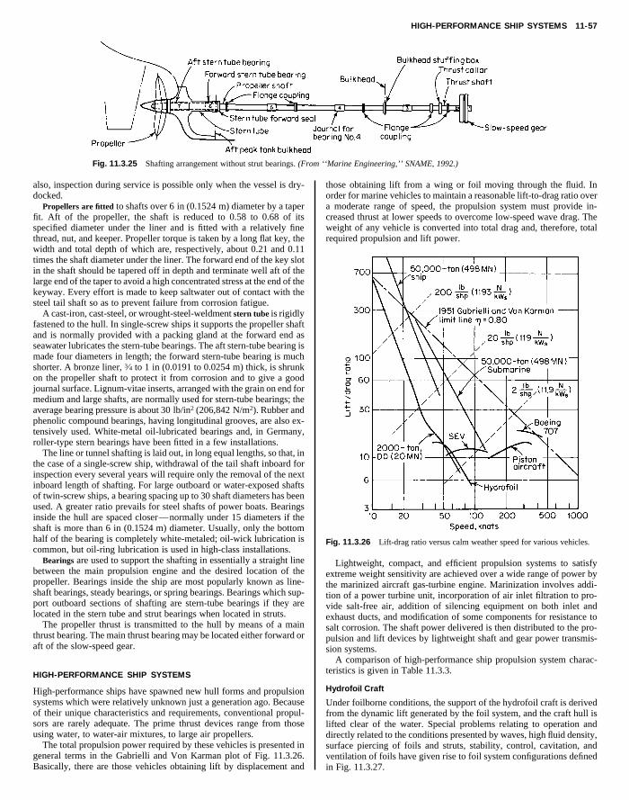
HIGH-PERFORMANCE SHIP SYSTEMS 11-57
Fig. 11.3.25 Shafting arrangement without strut bearings. (From ‘‘Marine Engineering,’’ SNAME, 1992.)
also, inspection during service is possible only when the vessel is dry-docked.
Propellers are fitted to shafts over 6 in (0.1524 m) diameter by a taperfit. Aft of the propeller, the shaft is reduced to 0.58 to 0.68 of itsspecified diameter under the liner and is fitted with a relatively finethread, nut, and keeper. Propeller torque is taken by a long flat key, thewidth and total depth of which are, respectively, about 0.21 and 0.11times the shaft diameter under the liner. The forward end of the key slotin the shaft should be tapered off in depth and terminate well aft of thelarge end of the taper to avoid a high concentrated stress at the end of the
those obtaining lift from a wing or foil moving through the fluid. Inorder for marine vehicles to maintain a reasonable lift-to-drag ratio overa moderate range of speed, the propulsion system must provide in-creased thrust at lower speeds to overcome low-speed wave drag. Theweight of any vehicle is converted into total drag and, therefore, totalrequired propulsion and lift power.
Copyright (C) 1999 by The McGraw-Hill Companies, Inc. All rights reserved. Use ofthis product is subject to the terms of its License Agreement. Click here to view.
keyway. Every effort is made to keep saltwater out of contact with thesteel tail shaft so as to prevent failure from corrosion fatigue.
A cast-iron, cast-steel, or wrought-steel-weldment stern tube is rigidlyfastened to the hull. In single-screw ships it supports the propeller shaftand is normally provided with a packing gland at the forward end asseawater lubricates the stern-tube bearings. The aft stern-tube bearing ismade four diameters in length; the forward stern-tube bearing is muchshorter. A bronze liner, 3⁄4 to 1 in (0.0191 to 0.0254 m) thick, is shrunkon the propeller shaft to protect it from corrosion and to give a goodjournal surface. Lignum-vitae inserts, arranged with the grain on end formedium and large shafts, are normally used for stern-tube bearings; theaverage bearing pressure is about 30 lb/in2 (206,842 N/m2). Rubber andphenolic compound bearings, having longitudinal grooves, are also ex-tensively used. White-metal oil-lubricated bearings and, in Germany,roller-type stern bearings have been fitted in a few installations.
The line or tunnel shafting is laid out, in long equal lengths, so that, inthe case of a single-screw ship, withdrawal of the tail shaft inboard forinspection every several years will require only the removal of the nextinboard length of shafting. For large outboard or water-exposed shaftsof twin-screw ships, a bearing spacing up to 30 shaft diameters has beenused. A greater ratio prevails for steel shafts of power boats. Bearingsinside the hull are spaced closer—normally under 15 diameters if theshaft is more than 6 in (0.1524 m) diameter. Usually, only the bottomhalf of the bearing is completely white-metaled; oil-wick lubrication iscommon, but oil-ring lubrication is used in high-class installations.
Bearings are used to support the shafting in essentially a straight linebetween the main propulsion engine and the desired location of thepropeller. Bearings inside the ship are most popularly known as line-shaft bearings, steady bearings, or spring bearings. Bearings which sup-port outboard sections of shafting are stern-tube bearings if they arelocated in the stern tube and strut bearings when located in struts.
The propeller thrust is transmitted to the hull by means of a mainthrust bearing. The main thrust bearing may be located either forward oraft of the slow-speed gear.
HIGH-PERFORMANCE SHIP SYSTEMS
High-performance ships have spawned new hull forms and propulsionsystems which were relatively unknown just a generation ago. Becauseof their unique characteristics and requirements, conventional propul-sors are rarely adequate. The prime thrust devices range from thoseusing water, to water-air mixtures, to large air propellers.
The total propulsion power required by these vehicles is presented ingeneral terms in the Gabrielli and Von Karman plot of Fig. 11.3.26.Basically, there are those vehicles obtaining lift by displacement and
Fig. 11.3.26 Lift-drag ratio versus calm weather speed for various vehicles.
Lightweight, compact, and efficient propulsion systems to satisfyextreme weight sensitivity are achieved over a wide range of power bythe marinized aircraft gas-turbine engine. Marinization involves addi-tion of a power turbine unit, incorporation of air inlet filtration to pro-vide salt-free air, addition of silencing equipment on both inlet andexhaust ducts, and modification of some components for resistance tosalt corrosion. The shaft power delivered is then distributed to the pro-pulsion and lift devices by lightweight shaft and gear power transmis-sion systems.
A comparison of high-performance ship propulsion system charac-teristics is given in Table 11.3.3.
Hydrofoil Craft
Under foilborne conditions, the support of the hydrofoil craft is derivedfrom the dynamic lift generated by the foil system, and the craft hull islifted clear of the water. Special problems relating to operation anddirectly related to the conditions presented by waves, high fluid density,surface piercing of foils and struts, stability, control, cavitation, andventilation of foils have given rise to foil system configurations definedin Fig. 11.3.27.

11-58 MARINE ENGINEERING
Table 11.3.3 U.S. Navy High-Performance Ship Propulsion System Characteristics
Ship Engine Propulsor /lift
Hydrofoil, PHM, 215 tons (2.1 MN), 50 knots Foilborne: one LM-2500 GT, 22,000 bhp (15,405kWB), 3,600 r/min
Foilborne: one 2-stage axial-flow waterjet, twin aftstrut inlets
Surface-effect ship, SES-200, 195 tons (1.94 MN),30 1 knots
Propulsion: two 16V-149TI diesel, 1,600 bhp (1,193kWB)
Lift: two 8V-92TI diesel, 800 bhp (597 kWB)
Two waterjet units
Two double-inlet centrifugal lift fans
Air-cushion vehicle, LCAC, 150 tons (1.49 MN),50 knots
Propulsion and lift: four TF-40B GT, 3,350 bhp(2,498 kWB), 15,400 r/min
Two ducted-air propellers, 12 ft (3.66 m) dia., 1,250r/min; four double-entry centrifugal lift fans, 1,900r/min
SWATH, SSP, 190 tons (1.89 MN), 25 knots Propulsion: two T-64 GT, 3,200 bhp (2,386 kWB),1,000 r/min at output of attached gearbox
Two subcavitating controllable-pitch propellers, 450r/min
The hydrofoil craft has three modes of operation: hullborne, takeoff,and foilborne. The thrust and drag forces involved in hydrofoil operationare shown in Fig. 11.3.28. Design must be a compromise between thevaried requirements of these operating conditions. This may be difficult,
need for supercavitating propellers at operating speeds over 50 knots.Two sets of propellers may be needed in such a case, one for hullborneoperation and the other for foilborne operation. The selection of a sur-face-piercing or a fully submerged foil design is determined from speci-fied operating conditions and the permissible degree of complexity. Asurface-piercing system is inherently stable, as a deviation from the equi-librium position of the craft results in corrective lift forces. Fully sub-merged foil designs, on the other hand, provide the best lift-drag ratio butare not stable by themselves and require a depth-control system forsatisfactory operation. Such a control system, however, permits opera-
Copyright (C) 1999 by The McGraw-Hill Companies, Inc. All rights reserved. Use ofthis product is subject to the terms of its License Agreement. Click here to view.
Fig. 11.3.27 Some foil arrangements and sections.
as with propeller design, where maximum thrust is often required attakeoff speed (normally about one-half the operating speed). A pro-peller designed for maximum efficiency at takeoff will have a smallerefficiency at design speeds, and vice versa. This is complicated by the
Fig. 11.3.28 Thrust and drag forces for a typical hydrofoil.
tion of the submerged-foil design in higher waves.
Flexible SkirtSkegs or side walls
Fig. 11.3.29 Two configurations of the surface-effect principle.
Surface-Effect Vehicles (SEV)
The air-cushion-supported surface-effect ship (SES) and air-cushion vehi-cle (ACV) show great potential for high-speed and amphibious opera-tion. Basically, the SEV rides on a cushion of air generated and main-tained in the space between the vehicle and the surface over which itmoves or hovers. In the SES, the cushion is captured by rigid sidewalls
Fig. 11.3.30 Comparison of power requirements: SES versus ACV.

UPPER ATMOSPHERE 11-59
and flexible skirts fore and aft. The ACV has a flexible seal or skirt allaround. Figure 11.3.29 illustrates two configurations of the surface-effect principle.
Since the ACV must rise above either land or water, the propul-sors use only air for thrust, requiring a greater portion of the totalpower allocated to lift than in the SES design as shown in Fig.11.3.30.
While SES technology has greatly improved the capability of am-phibious landing vehicles, it is rapidly being developed for high-speedlarge cargo vessels.
CARGO SHIPS
The development of containerization in the 1950s sparked a growth inship size. More efficient cargo-handling methods and the desire to re-duce transit time led to the emergence of the high-speed containervessel.
The Container Vessel
Because of low fuel costs in the 1950s and 1960s, early container vesseldesign focused on higher speed and container capacity. Rising fuel costs
O. M
Copyright (C) 1999 by The McGraw-Hill Companies, Inc. All rights reserved. Use ofthis product is subject to the terms of its License Agreement. Click here to view.
Small Water-Plane Area Twin Hull
The SWATH, configured to be relatively insensitive to seaway motions,gains its buoyant lift from two parallel submerged, submarinelike hullswhich support the main hull platform through relatively small verticalstruts. In this configuration, a propulsion arrangement choice must bewith regard to the location of the main engines: lower hull with thepropulsor or upper hull with a suitable transmission system. In the U.S.Navy’s semisubmerged platform (SSP), power from two independentlyoperated gas turbines is transmitted down each aft strut by a group ofthree wide-belt chain drives with speed reduction to deliver 450 r/min tothe propellers. By contrast, the 3,400-ton (33.87-MN), 11-knotT-AGOS 19 series SWATH vessels employ diesel-electric drive, withboth motors and propulsors in the lower hull.
11.4 AERby M. W
REFERENCES: National Advisory Committee for Aeronautics, Technical Reports(designated NACA-TR with number), Technical Notes (NACA-TN with number),
and Technical Memoranda (NACA-TM with number). British Aeronautical Re-search Committee Reports and Memoranda (designated Br. ARC-R & M withnumber). Ergebnisse der Aerodynamischen Versuchsanstalt zu Gottingen. Diehl,‘‘Engineering Aerodynamics,’’ Ronald. Reid, ‘‘Applied Wing Theory,’’McGraw-Hill. Durand, ‘‘Aerodynamic Theory,’’ Springer. Prandtl-Tietjens,‘‘Fundamentals of Hydro- and Aeromechanics,’’ and ‘‘Appliemechanics,’’ McGraw-Hill. Goldstein, ‘‘Modern Developmnamics,’’ Oxford. Millikan, ‘‘Aerodynamics of the Airplane,’’‘‘Theory of Flight,’’ McGraw-Hill. Hoerner, ‘‘Aerodynamishifted emphasis toward ship characteristics which enhanced reducedoperating costs, particularly as affected by fuel usage and trade routecapacity. By the early 1980s, ships were generally sized for TEU(twenty-foot-equivalent-unit) capacity less than 2,500 and speeds ofabout 20 knots, lower if fuel was significant in the overall operatingcosts. Largely a function of the scale of trade route capacity, theweighted average full containership size is on the order of 1,000 TEU.The larger the trade capacity, the larger the containerships operating theroute. However, many trade route scales do not support even moder-ately sized containership service.
The on deck and under deck container capacity varies with the type ofvessel, whether a lift on/lift off vessel, a bulk carrier equipped for con-tainers, or a roll on/roll off vessel. Extensive studies have been conductedto optimize the hull form and improve the operating efficiency for themodern containership.
NAUTICS. Jenkins
sound in the fluid. The velocity range below the local speed of sound iscalled the subsonic regime. Where the velocity is above the local speed
of sound, the flow is said to be supersonic. The term transonic refers toflows in which both subsonic and supersonic regions are present. Thehypersonic regime is that speed range usually in excess of five times thespeed of sound.OSPHERE
osphere of Table 11.4.1 is a revised U.S. Standard
d Hydro- and Aero-ents in Fluid Dy-Wiley. Von Mises,
c Drag,’’ Hoerner.
STANDARD ATM
The standard atm
Glauert, ‘‘The Elements of Airfoil and Airscrew Theory,’’ Cambridge. Milne-Thompson, ‘‘Theoretical Hydrodynamics,’’ Macmillan. Munk, ‘‘Fluid Dynamicsfor Aircraft Designers,’’ and ‘‘Principles of Aerodynamics,’’ Ronald. Abraham,‘‘Structural Design of Missiles and Spacecraft,’’ McGraw-Hill. ‘‘U.S. StandardAtmosphere, 1962,’’ U.S. Government Printing Office.DEFINITIONS
Aeronautics is the science and art of flight and includes the operation ofheavier-than-air aircraft. An aircraft is any weight-carrying device de-signed to be supported by the air, either by buoyancy or by dynamicaction. An airplane is a mechanically driven fixed-wing aircraft, heavierthan air, which is supported by the dynamic reaction of the air against itswings. A helicopter is a kind of aircraft lifted and moved by a largepropeller mounted horizontally above the fuselage. It differs from theautogiro in that this propeller is turned by motor power and there is noauxiliary propeller for forward motion. A ground-effect machine (GEM)is a heavier-than-air surface vehicle which operates in close proximityto the earth’s surface (over land or water), never touching except at rest,being separated from the surface by a cushion or film of air, howeverthin, and depending entirely upon aerodynamic forces for propulsionand control.
Aerodynamics is the branch of aeronautics that treats of the motion ofair and other gaseous fluids and of the forces acting on solids in motionrelative to such fluids. Aerodynamics falls into velocity ranges, depend-ing upon whether the velocity is below or above the local speed of
Atmosphere, adapted by the United States Committee on Extension tothe Standard Atmosphere (COESA) in 1962.
The values given up to about 65,000 ft are designated as standard.The region from 65,000 to 105,000 ft is designated proposed standard.U.S. Standard Atmosphere, 1962, gives data out to 2,320,000 ft; how-ever, the region from 105,000 to 295,000 ft is designated tentative, andthat portion of the atmosphere above 295,000 ft is termed speculative.
The assumed sea-level conditions are: pressure, p0 5 29.91 in(760 mm Hg) 5 2,116.22 lb/ft2; mass density, r0 5 0.002378 slugs/ft3
(0.001225 g/cm3); T0 5 59°F (15°C).
UPPER ATMOSPHERE
High-altitude atmospheric data have been obtained directly from bal-loons, sounding rockets, and satellites and indirectly from observationsof meteors, aurora, radio waves, light absorption, and sound effects. Atrelatively low altitudes, the earth’s atmosphere is, for aerodynamic pur-poses, a uniform gas. Above 250,000 ft, day and night standards differbecause of dissociation of oxygen by solar radiation. This difference indensity is as high as 35 percent, but it is usually aerodynamically negli-gible above 250,000 ft since forces here will become less than 0.05percent of their sea-level value for the same velocity.
Temperature profile of the COESA atmosphere is given in Fig. 11.4.1.From these data, other properties of the atmosphere can be calcu-lated.

11-60 AERONAUTICS
Table 11.4.1 U.S. Standard Atmosphere, 1962
Pressure Speed ofAltitude Temp ratio, Density ratio, sound Vs,
h, ft* T, °F† p /p0 r /r0 (r0 /r)0.5 ft /s‡
0 59.00 1.0000 1.0000 1.000 1,1165,000 41.17 0.8320 0.8617 1.077 1,097
10,000 23.34 0.6877 0.7385 1.164 1,07715,000 5.51 0.5643 0.6292 1.261 1,05720,000 2 12.62 0.4595 0.5328 1.370 1,03625,000 2 30.15 0.3711 0.4481 1.494 1,015
Speed in aeronautics may be given in knots (now standard for USAF,USN, and FAA), miles per hour, feet per second, or metres per second.The international nautical mile 5 6,076.1155 ft (1,852 m). The basicrelations are: 1 knot 5 0.5144 m/s 5 1.6877 ft/s 5 1.1508 mi/h. Foradditional conversion factors see Sec. 1. Higher speeds are often givenas Mach number, or the ratio of the particular speed to the speed of soundin the surrounding air. For additional data see ‘‘Supersonic and Hyper-sonic Aerodynamics’’ below.
Axes The forces and moments acting on an airplane (and the resul-tant velocity components) are referred to a set of three mutually perpen-
Copyright (C) 1999 by The McGraw-Hill Companies, Inc. All rights reserved. Use ofthis product is subject to the terms of its License Agreement. Click here to view.
30,000 2 47.99 0.2970 0.3741 1.635 99535,000 2 65.82 0.2353 0.3099 1.796 97336,089 2 69.70 0.2234 0.2971 1.835 96840,000 2 69.70 0.1851 0.2462 2.016 96845,000 2 69.70 0.1455 0.1936 2.273 96850,000 2 69.70 0.1145 0.1522 2.563 96855,000 2 69.70 0.09001 0.1197 2.890 96860,000 2 69.70 0.07078 0.09414 3.259 96865,000 2 69.70 0.05566 0.07403 3.675 96865,800 2 69.70 0.05356 0.07123 3.747 96870,000 2 67.30 0.04380 0.05789 4.156 97175,000 2 64.55 0.03452 0.04532 4.697 97480,000 2 61.81 0.02725 0.03553 5.305 97785,000 2 59.07 0.02155 0.02790 5.986 98190,000 2 56.32 0.01707 0.02195 6.970 98495,000 2 53.58 0.01354 0.01730 7.600 988
100,000 2 50.84 0.01076 0.01365 8.559 991
* 3 0.3048 5 metres.† 3 (°F 2 32)/1.8 5 °C.‡ 3 0.3048 5 m/s.
Pressure and Density For all practical purposes, both decrease ex-ponentially with altitude. The variations in T (Fig. 11.4.1) are accompa-nied by slight inflections in the curves of p and r, but the deviationsfrom a mean curve are far less than the scatter in test data from varioussources. For altitudes above 100,000 ft, pressure and density may beapproximated by
log p0 /p 5 0.00001910h 1 0.0140log r0 /r 5 0.00001890h 2 0.1000
where h is in ft. At h 5 320,000 ft, or about 60 mi (96 km), p and r areabout one-millionth of the sea-level values.
Fig. 11.4.1 Temperature as a function of altitude. (COESA.)
dicular axes having the origin at the airplane center of gravity (cg) andmoving with the airplane. Three sets of axes are in use. The basicdifference in these is in the direction taken for the longitudinal, or x,axis, as follows:
Wind axes: The x axis lies in the direction of the relative wind. This isthe system most commonly used, and the one used in this section. It isshown on Fig. 11.4.2.
Body axes: The x axis is fixed in the body, usually parallel to thethrust line.
Stability axes: The x axis points in the initial direction of flight. Thisresults in a simplification of the equations of motion.
Absolute Coefficients Aerodynamic force and moment data areusually presented in the form of absolute coefficients. Examples offorce coefficients are: lift CL 5 L/qS; drag CD 5 D/qS; side force CY 5Y/qS; where q is the dynamic pressure 1⁄2rV 2, r 5 air mass-density, andV 5 air speed. Examples of moment coefficients are Cm 5 M/qSc; rollCl 5 L/qSb; and yaw Cn 5 N/qSb; where c 5 mean wing chord and b 5wing span.
Section Coefficients NACA basic test data on wing sections areusually given in the form of section lift coefficient Cl and section dragcoefficient Cd . These apply directly to an infinite aspect ratio or totwo-dimensional flow, but aspect-ratio and lift-distribution correctionsare necessary in applying to a finite wing. For a wing having an ellipti-cal lift distribution, CL 5 (p/4)Cl , where Cl is the centerline value of thelocal lift coefficient.
Fig. 11.4.2 Wind axes.
SUBSONIC AERODYNAMIC FORCES
When an airfoil is moved through the air, the motion produces a pres-sure at every point of the airfoil which acts normal to the surface. Inaddition, a frictional force tangential to the surface opposes the motion.The sum of these pressure and frictional forces gives the resultant forceR acting on the body. The point at which the resultant force acts isdefined as the center of pressure, c.p. The resultant force R will, in gen-eral, be inclined to the airfoil and the relative wind velocity V. It isresolved (Fig. 11.4.3) either along wind axes into
L 5 lift 5 component normal to VD 5 drag or resistance 5 component along V, or along
body axes into

AIRFOILS 11-61
N 5 normal force 5 component perpendicular to airfoil chordT 5 tangential force 5 component along airfoil chord
Instead of specifying the center of pressure, it is convenient to specifythe moment of the air forces about the so-called aerodynamic center,a.c. This point lies at a distance a (about a quarter-chord length) back ofthe leading edge of the airfoil and is defined as the point about which themoment of the air forces remains constant when the angle of attack a ischanged. Such a point exists for every airfoil. The force R acting at thec.p. is equivalent to the same force acting at the a.c. plus a moment equal
AIRFOILS
Applying Bernoulli’s equation to the flow around a body, if p representsthe static pressure, i.e., the atmospheric pressure in the undisturbed air,and if V is superposed as in Fig. 11.4.4 and if p1 , V1 represent thepressure and velocity at any point 1 at the surface of the body,
p 1 1⁄2rV 2 5 p1 1 1⁄2rV 21
The maximum pressure occurs at a point s on the body at which thevelocity is zero. Such a point is defined as the stagnation point. The
Copyright (C) 1999 by The McGraw-Hill Companies, Inc. All rights reserved. Use ofthis product is subject to the terms of its License Agreement. Click here to view.
to that force times the distance between the c.p. and the a.c. (see Fig.11.4.3). The location of the aerodynamic center, in terms of the chord cand the section thickness t, is given for NACA 4- and 5-digit seriesairfoils approximately by
a/c 5 0.25 2 0.40(t/c)2
The distance x c.p. from the leading edge to the center of pressureexpressed as a fraction of the chord is, in terms of the moment Mc/4
about the quarter-chord point,
Mc/4 5 (1⁄4 2 xc.p.) ? cN
xc.p. 51
42
Mc/4
cN
From dimensional analysis it can be seen that the air force on a body oflength dimension l moving with velocity V through air of density r canbe expressed as
F 5 w ? rV 2l2
where w is a coefficient that depends upon all the dimensionless factorsof the problem. In the case of a wing these are:
1. Angle of attack a, the inclination between the chord line and thevelocity V
2. Aspect ratio A 5 b/c, where b is the span and c the mean chord ofthe wing
3. Reynolds number Re 5 rVl/m, where m is the coefficient of dy-namic viscosity of air
4. Mach number V/Vs , where Vs is the velocity of sound5. Relative surface roughness6. Relative turbulence
The dependence of the force coefficient w upon a and A can be theoreti-cally determined; the variation of w with the other parameters must beestablished experimentally, i.e., by model tests.
Fig. 11.4.3 Forces acting on an airfoil. (a) Actual forces; (b) equivalent forcesthrough the aerodynamic center plus a moment.
maximum pressure increase occurs at this point and is
ps 2 p 5 1⁄2rV 2
This is called the stagnation pressure, or dynamic pressure, and is de-noted by q. It is customary to express all aerodynamic forces in terms of1⁄2rV 2, hence
F 5 1⁄2wrV 2l2 5 qwl2
For the case of a wing, the forces and moments are expressed as
Lift 5 L 5 CL1⁄2rV 2S 5 CLqS
Drag 5 D 5 CD1⁄2rV 2S 5 CDqS
Moment 5 M 5 CM1⁄2rV 2Sc 5 CMqSc
where S 5 wing area and c 5 wing chord.
V
V1, p1
P
S
Fig. 11.4.4 Fluid flow around an airfoil.
The lift produced can be determined from the intensity of the circula-tory flow or circulation G by the relation L9 5 rV G, where L9 is the liftper unit width of wing. In a wing of infinite aspect ratio, the flow istwo-dimensional and the lift reaction is at right angles to the line ofrelative motion. The lift coefficient is a function of the angle of attack a,and by mathematical analysis CL 5 2p sin a, which for small anglesbecomes CL 5 2pa. Experiments show that CL 5 2ph(a 2 a0), wherea0 is the angle of attack corresponding to zero lift. h ' 1 2 0.64(t/c),where t is airfoil thickness.
In a wing of finite aspect ratio, the circulation flow around the wingcreates a strong vortex trailing downstream from each wing tip (Fig.
V
wi
Fig. 11.4.5 Vortex formation at wing tips.
11.4.5). The effect of this is that the direction of the resultant velocity atthe wing is tilted downward by an induced angle of attack ai 5 wi /V (Fig.11.4.6). If friction is neglected, the resultant force R is now tilted to therear by this same angle ai . The lift force L is approximately the same asR. In addition, there is also a drag component Di , called the induceddrag, given by
Di 5 L tan ai 5 Lwi /V

11-62 AERONAUTICS
For a given geometrical angle of attack a the effective angle of attack hasbeen reduced by ai , and thus
CL 5 2ph(a 2 a0 2 ai)
an airfoil is a small value of the minimum profile-drag coefficient and alarge value of CL /CD .
The moment characteristics of a wing are obtainable from the curveof the center of pressure as a function of a or by the moment coefficienttaken about the aerodynamic center CMa.c. as a function of CL . A forwardmotion of the c.p. as a is increased corresponds to an unstable wingsection. This instability is undesirable because it requires a large down-load on the tail to counteract it.
Copyright (C) 1999 by The McGraw-Hill Companies, Inc. All rights reserved. Use ofthis product is subject to the terms of its License Agreement. Click here to view.
wi
Fig. 11.4.6 Induced angle of attack.
According to the Lanchester-Prandtl theory, for wings having an ellipticallift distribution
ai 5 wi /V 5 CL /pA radDi 5 L2/pb2q and CDi 5 Di /qS 5 C 2
L /pA
where b 5 span of wing and A 5 b2/S 5 aspect ratio of wing. Theseresults also apply fairly well to wings not differing much from theelliptical shape. For square tips, correction factors are required:
ai 5CL
pA(1 1 t) where t 5 0.05 1 0.02A
for A , 12CDi 5
C 2L
pA(1 1 s) where s 5 0.01A 2 0.01
These formulas are the basis for transforming the characteristics ofrectangular wings from an aspect ratio A1 to an aspect ratio A2:
a2 5 a1 157.3CL
pS1 1 t2
A2
21 1 t1
A1D deg
CD2 5 CD1 1C 2
L
pS1 1 s2
A2
21 1 s1
A1D
For elliptical wings the values of t and s are zero. Most wing-sectiondata are given in terms of aspect ratios 6 and `. For other values, thepreceding formulas must be used.
Characteristics of Airfoils Airfoil characteristics are expressed interms of the dimensionless coefficients CL , CD , and CM and the angle ofattack a. The NACA presents the results for wings of aspect ratio 6 andalso corrected to aspect ratio ` (see Fig. 11.4.10).
The lift coefficient CL is a linear function of the angle of attack up to acritical angle called the stalling angle (Fig. 11.4.7). The maximum liftcoefficient CLmax which can be reached is one of the important character-istics of a wing because it determines the landing speed of theairplane.
The drag of a wing is made up of two components: the profile drag D0
and the induced drag Di . The profile drag is due principally to surfacefriction. At aspect ratio ` or at zero lift the induced drag is zero, andthus the entire drag is profile drag. In Fig. 11.4.8 the coefficient ofinduced drag CDi 5 C 2
L /pA is also plotted. The difference CD 2 CDi 5CD0 , the profile-drag coefficient. Among the desirable characteristics of
Fig. 11.4.7 Stalling angle of an airfoil.
Fig. 11.4.8 Polar-diagram plot of airfoil data.
The characteristics of a wing section (Fig. 11.4.9) are determinedprincipally by its mean camber line, i.e., the curvature of the median lineof the profile, and secondly by the thickness distribution along thechord. In the NACA system of designation, when a four-digit number isused such as 2412, the significance is always first digit 5 maximumcamber in percent of chord, second digit 5 location of position ofmaximum camber in tenths of chord measured from the leading edge(that is, 4 stands for 40 percent), and the last two figures indicate themaximum thickness in percent of chord. The NACA five-digit system isexplained in NACA-TR 610.
Fig. 11.4.9 Characteristics of a wing section.
Selection of Wing Section
In selecting a wing section for a particular airplane the following factorsare generally considered:
1. Maximum lift coefficient CLmax
2. Minimum drag coefficient CDmin
3. Moment coefficient at zero lift Cm0
4. Maximum value of the ratio CL /CD
For certain special cases it is necessary to consider one or morefactors from the following group:
5. Value of CL for maximum CL /CD
6. Value of CL for minimum profile drag

AIRFOILS 11-63
Fig. 11.4.10 Properties of an airfoil section.
7. Maximum value of C L3/2/CD
8. Maximum value of C L1/2/CD
9. Type of lift curve peak (stall characteristics)10. Drag divergence Mach number MDD
Characteristics of airfoil sections are given in NACA-TR 586, 647,669, 708, and 824. Figure 11.4.10 gives data on two typical sections:0006 is often used for tail surfaces, and 4415 is especially suitable forthe wings of subsonic airplanes. For Mach numbers greater than 0.6 thinwings must be used.
The dimensionless coefficients C and C are functions of the Rey-
20,00.5
variation of the drag coefficient for a smooth flat plate for laminar andturbulent flow, respectively, and also for the transition region.
which the distribution of thickness along the chord is so selected as to
Copyright (C) 1999 by The McGraw-Hill Companies, Inc. All rights reserved. Use ofthis product is subject to the terms of its License Agreement. Click here to view.
L D
nolds number Re 5 rVl/m. For wings, the characteristic length l is takento be the chord. In standard air at sea level
Re 5 6,378Vft/s ? lft 5 9,354Vmi/h ? lft
For other heights, multiply by the coefficient K 5 (r/m)/(r0 /m0). Valuesof K are as follows:
Altitude, ft* 0 5,000 10,000 15,000K 1.000 0.884 0.779 0.683
* 3 0.305 5 m.
The variation of CL and CD with the Reynolds number is known asscale effect. These are shown in Figs. 11.4.11 and 11.4.12 for sometypical airfoils. Figure 11.4.12 shows in dashed lines also the theoretical
00 25,000 30,000 40,000 50,000 60,00095 0.515 0.443 0.300 0.186 0.116
Fig. 11.4.12 Scale effect on minimum profile-drag coefficient.
In addition to the Reynolds number, airfoil characteristics also de-pend upon the Mach number (see ‘‘Supersonic and Hypersonic Aerody-namics’’ below).
Laminar-flow Wings NACA developed a series of low-drag wings in
maintain laminar flow over as much of the wing surface as possible.The low-drag wing under controlled conditions of surface smooth-
ness may have drag coefficients about 30 percent lower than thoseobtained on normal conventional wings. Low-drag airfoils are so sensi-tive to roughness in any form that the full advantage of laminar flow is
Fig. 11.4.11 Scale effect on section maximum lift coefficient.
unobtainable.Transonic Airfoils At airplane Mach numbers of about M 5 0.75,
normal airfoil sections begin to show a greater drag, which increasessharply as the speed of sound is approached. Airfoil sections known astransonic airfoils have been developed which significantly delay thisdrag rise to Mach numbers of 0.9 or greater (Fig. 11.4.13). Advantage

11-64 AERONAUTICS
may also be taken of these airfoil sections by increasing the thickness ofthe airfoil at a given Mach number without suffering an increase in drag.
Wing sweepback (Fig. 11.4.14) or sweepforward also delays the onsetof the drag rise to higher Mach numbers. The flow component normal tothe wing leading edge, M cos G, determines the effective Mach numberfelt by the wing. The parallel component, M sin G, does not significantlyinfluence the drag rise. Therefore for a flight Mach number M, the wingsenses it is operating at a lower Mach number given by M cos G.
Subsonic
moment (2 Cm) which must be trimmed out by a download on the tail,and this download reduces CLmax . The correction is DCLmax (trim) 5DCmo(l/c), where l/c is the tail length in mean chords.
Boundary-Layer Control (BLC) This includes numerous schemesfor (1) maintaining laminar flow in the boundary layer in the flow over a
Copyright (C) 1999 by The McGraw-Hill Companies, Inc. All rights reserved. Use ofthis product is subject to the terms of its License Agreement. Click here to view.
CD
0 M 1.0
Drag riseMach number
airfoil
Transonicairfoil
Fig. 11.4.13 Drag rise delay due to transonic section.
CD
No sweep
M
Wing
M sin GM cos G
G
With sweep
0 Mach number
Drag rise Mach number
1.0
Fig. 11.4.14 Influence of wing sweepback on drag rise Mach number.
Flaps and Slots
The maximum lift of a wing can be increased by the use of slots on theleading edge or flaps on the trailing edge. Fixed slots are formed byrigidly attaching a curved sheet of metal or a small auxiliary airfoil tothe leading edge of the wing. The trailing-edge flap is used to giveincreased lift at moderate angles of attack and to increase CLmax . Theo-retical analyses of the effects are given in NACA-TR 938 and Br. ARC-R&M 1095. Flight experience indicates that the four types shown in Fig.11.4.15 have special advantages over other known types. Values ofCLmax for these types are shown in Table 11.4.2. All flaps cause a diving
Table 11.4.2 Flaps*
Section Finite wingCLmax CLmax
Type of flap (approx) (approx) Remarks
Plain 2.4 1.9 Cf /c 5 0.20. Sensitiveto leakage betweenflap and wing.
Split 2.6 2.0 Cf /c 5 0.20. Simplesttype of flap.
Single slotted 2.83.0
2.22.4
Cf /c 5 0.25. Shape ofslot and location ofdeflected flap are crit-ical.
Double slotted 3.03.4
2.42.7
Cf /c 5 0.25. Shape ofslot and location ofdeflected flap are crit-ical.
* The data is for wing thickness t /c 5 0.12 or 0.15. Lift increment is dependent on theleading-edge radius of the wing.
Fig. 11.4.15 Trailing-edge flaps: (1) plain flap; (2) split flap; (3) single-slottedflap; (4) double-slotted flap (retracted); (5) double-slotted flap (extended).
wing or (2) preventing flow separation. Schemes in the first category tryto obtain the lower frictional drag of laminar flow either by providingfavorable pressure gradients, as in the NACA ‘‘low-drag’’ wings, or byremoving part of the boundary layer. The boundary-layer thickness canbe partially controlled by the use of suction applied either to spanwiseslots or to porous areas. The flow so obtained approximates the laminarskin-friction drag coefficients (see Fig. 11.4.12). Schemes in the secondcategory try to delay or improve the stall. Examples are the leading-edge slot, slotted flaps, and various forms of suction or blowing appliedthrough transverse slots. The slotted flap is a highly effective form ofboundary-layer control that delays flow separation on the flap.
CL
Angle of attack a
Nozzle
Withblowing
No blowing
o
Fig. 11.4.16 Influence of spanwise blowing.
Spanwise Blowing Another technique for increasing the lift froman aerodynamic surface is spanwise blowing. A high-velocity jet of airis blown out along the wing. The location of the jet may be parallel toand near the leading edge of the wing to prevent or delay leading-edgeflow separation, or it may be slightly behind the juncture of the trailing-edge flap to increase the lift of the flap. Power for spanwise blowing issensitive to vehicle configuration and works most efficiently on sweptwings. Other applications of this technique may include local blowingon ailerons or empennage surfaces (Fig. 11.4.16).
The pressure distributions on a typical airfoil are shown in Fig.11.4.17. In this figure the ratio p/q is given as a function of distancealong the chord. In Fig. 11.4.18 the effect of addition of an externalairfoil flap is shown.

AIRFOILS 11-65
Upper Surface
altitude (Fig. 11.4.19). If PTa . PTr , the excess horsepower can be usedeither for horizontal acceleration to a higher speed or for climbing. Themaximum speed Vmax occurs when PTa 5 PTr . The rate of climb isdetermined by the equation dh/dt 5 550(PTa 2 PTr)/W. To calculate the
Copyright (C) 1999 by The McGraw-Hill Companies, Inc. All rights reserved. Use ofthis product is subject to the terms of its License Agreement. Click here to view.
Lower Surface
Fig. 11.4.17 Pressure distribution over a typical airfoil.
Upper
Lower
Fig. 11.4.18 Pressure distribution on an airfoil-flap combination.
Airplane Performance
In horizontal flight the lift of the wings must be equal to the weight of theairplane, or L 5 W, where W is the gross weight, lb (kg). This equationdetermines the minimum horizontal speed of an airplane since
W 5 CLmax1⁄2rV 2
minS or Vmin 5 √2W/CLmaxrS
This corresponds to the landing speed without power, or the stallingspeed.
In uniform horizontal flight the propeller thrust T must be exactlyequal to the drag of the airplane, or T 5 D. Then TV 5 power availablefrom the propeller and DV 5 power required for overcoming the drag ofthe airplane; for horizontal flight TV 5 DV. If the airplane climbs at arate dh /dt, where h 5 height, then an additional power 5 W (dh/dt) isrequired to increase the potential energy of the airplane. The equilib-rium condition becomes
TV 5 DV 1 W(dh/dt)
If the thrust power available PTa is measured in hp, D and W in lb, andV and dh/dt in ft/s,
PTa 51
550DV 1
1
550W(dh/dt) (11.4.1)
The thrust horsepower available PTa 5 hPa , where Pa 5 available enginehorsepower and h is the propeller efficiency. PTa is determined as afunction of V from the engine and propeller characteristics. The thrusthorsepower required to overcome the drag D is PTr 5 DV/550. The dragis the sum of the wing-profile drag D0 , the wing induced drag Di , andthe parasite drag of the other airplane parts Dp . D0 can be obtained fromwing-profile tests corrected to full-scale Reynolds number, Di from theinduced drag formula Di 5 L2/pqb2, and Dp by summation of the para-site drag components due to fuselage, tail surfaces, landing gear, etc.
From Eq. (11.4.1) the performance of an airplane can be obtainedeither graphically or analytically. In the graphical determination thecurves of power available and power required are plotted for a fixed
Fig. 11.4.19 Construction for determining airplane performance.
maximum velocity and rate of climb for another altitude, another set ofcurves of PTa and PTr versus V is constructed. At any altitude at whichthe air density is r and for a given angle of attack (corresponding to anunchanged lift /drag ratio), L/D 5 L0 /D0 . As the lift is equal to theweight, L 5 L0 5 W, therefore D 5 D0 and
PTr /PTr0 5 VD/V0D0 5 V/V0
But CL 5 CL0 and CL ? 1⁄2rV 2S 5 CL01⁄2r0V 0
2S. Therefore V/V0 5√r0 /r. From this relation, new curves of PTr versus V may be con-structed for various altitudes by multiplying both the ordinates and ab-scissas of the original curve by √r0 /r.
Figure 11.4.19 shows a performance chart for a 2,100-lb airplane.The maximum velocity at 10,000 ft altitude is 168.5 ft/s. At sea level(PTa 2 PTr)max 5 71 and the rate of climb is 71 3 33,000/2,100 51,120 ft/min. At 10,000 ft altitude the rate is 30 3 33,000/2,100 5470 ft/min.
When the curves of power required and power available becometangent to each other, there is only one speed at which the airplane canfly level and the rate of climb is zero. The corresponding altitude is theabsolute ceiling H. It can be determined from the curve of maximum rateof climb as a function of altitude when this is approximated by a straight
Fig. 11.4.20 Characteristic rate-of-climb curves.

11-66 AERONAUTICS
line (Fig. 11.4.20). The service ceiling hs is defined as the altitude atwhich the rate of climb is 100 ft/min. For a linear decrease of rate ofclimb the following approximations hold:
Absolute ceiling: H 5 r0h/(r0 2 r)
where r0 is the rate of climb at sea level and r is the rate of climb ataltitude h.
Service ceiling: hs 5 H(r0 2 100)/r0
Altitude climbed in t min,
0.50.60.8
where Ct is fuel consumption in lb/(lb thrust) ?hour, S is wing area in ft2,and r is the air density in slugs/ft3.
Parasite Drag
The drag of the nonlifting parts of an airplane is called the parasite drag.It consists of two components: the frictional and the eddy-makingdrag.
Frictional drag, or skin friction, is due to the viscosity of the fluid. It isthe force produced by the viscous shear in the layers of fluid immedi-ately adjacent to the body. It is always proportional to the wetted area,
Copyright (C) 1999 by The McGraw-Hill Companies, Inc. All rights reserved. Use ofthis product is subject to the terms of its License Agreement. Click here to view.
h 5 H(1 2 ek)
where k 5 2 r0t/H.Time to climb to altitude h,
t 5 2.303H
r0
logH
H 2 h
The maximum distance that an airplane can fly is called its range, andthe length of time that it can remain flying, its endurance. If W0 is theweight in pounds fully loaded and W1 the weight after having consumedits fuel at the rate of C lb/(bhp ? h), then for propeller-driven aircraft,
Range 5 863.5h
C?
L
D? log
W0
W1
mi
Endurance 5 750√W
Vc
?h
C?
L
DS 1
√W1
21
√W0
D hours
where h is the average propulsive efficiency and L/D 5 CL/CD is theratio of lift to drag. Vc is the cruising speed, mi/h, at any gross weightW, lb. See Table 11.4.3 for dimensions and performance of selectedairplanes.
Power Available The maximum efficiency hm and the diameter of apropeller to absorb a given power at a given speed and rpm are foundfrom a propeller-performance curve. The thrust horsepower at maxi-mum speed PTm is found from PTm 5 hm Pm . The thrust horsepower atany speed can be approximately determined from the ratios given in thefollowing table:
V/Vmax 0.20 0.30 0.40
PT/PTmHFixed-pitch propeller 0.29 0.44 0.57constant-rpm propeller 0.47 0.62 0.74
The brake horsepower of an engine decreases with increase of altitude.The variation of PT with altitude depends on engine and propeller char-acteristics with average values as follows:
h, ft 0 5,000 10,000 15,000 20,000 25,000
PT/PT0 (fixed pitch) 1.00 0.82 0.66 0.52 0.41 0.30PT/PT0 (controllablepitch) 1.00 0.85 0.71 0.59 0.48 0.38
Performance with Jet Thrust In all cases where jet thrust consti-
0 0.60 0.70 0.80 0.90 1.00 1.108 0.77 0.84 0.90 0.96 1.00 1.032 0.88 0.93 0.97 0.99 1.00 1.00
i.e., the total surface exposed to the air.Eddy-making drag, sometimes called form drag, is due to the distur-
bance or wake created by the body. It is a function of the shape of thebody.
The total drag of a body may be composed of the two components inany proportion, varying from almost pure skin friction for a plate edge-wise or a good streamline form to 100 percent form drag for a flat platenormal to the wind. A steamline form is a shape having very lowform drag. Such a form creates little disturbance in moving through afluid.
When air flows past a surface, the layer immediately adjacent to thesurface adheres to it, or the tangential velocity at the surface is zero. Inthe transition region near the surface, which is called the boundary layer,the velocity increases from zero to the velocity of the stream. When theflow in the boundary layer proceeds as if it were made up of laminaesliding smoothly over each other, it is called a laminar boundary layer. Ifthere are also irregular motions in the layers normal to the surface, it is aturbulent boundary layer. Under normal conditions the flow is laminar atlow Reynolds numbers and turbulent at high Re with a transition rangeof values of Re extending between 5 3 105 and 5 3 107. The profile-drag coefficients corresponding to these conditions are shown in Fig.11.4.12.
For laminar flow the friction-drag coefficient is practically indepen-dent of surface roughness and for a flat plate is given by the Blasiusequation,
CDF 5 2.656/√Re
The turbulent boundary layer is thicker and produces a greater fric-tional drag. For a smooth flat plate with a turbulent boundary layer
CDF 5 0.91/ log Re2.58
For rough surfaces the drag coefficients are increased (see von Karman,
Jour. Aeronaut. Sci., 1, no. 1, 1934). The drag coefficients as givenabove are based on projected area of a double-surfaced plane. If wettedarea is used, the coefficients must be divided by 2. The frictional drag isDF 5 CDF qS, where S is the projected area, or DF 5 1⁄2CDF qA, whereA is the wetted area.tutes either a part or all of the power source, it is necessary to usegraphical methods, plotting thrust and drag as functions of speed at eachaltitude to be investigated. The major thrust corrections are those due tolosses in (1) the air intake, (2) the ducting system, and (3) the tailpipe.(See Jet Propulsion and Aircraft Propellers.)
An excess thrust T, lb, at a speed V, mi/h, is equivalent to a thrusthorsepower PT 5 TV/375. The corresponding rate of climb is dh/dt 533,000PT/W 5 88TV/W.
For jet-driven aircraft, range and endurance can be determined from
Range 5 1.9285S 1
√rSD ?
1
Ct
?CL
1/2
CD
? (W01/2 2 W1
1/2) mi
and
Endurance 51
Ct
?CL
CD
? logSW0
W1D hours
Values of CDF for double-surfaced planes may be estimated from thefollowing tabulation:
Laminar flow (Blasius equation):
Re 10 102 103 104 105 106
CDF 0.838 0.265 0.0838 0.0265 0.0084 0.0265
Turbulent flow:
Re 105 106 107 108 109 1010
CDF 0.0148 0.0089 0.0060 0.0043 0.00315 0.0024
These are double-surface values which facilitate direct comparisonwith wing-drag coefficients based on projected area. For calculationsinvolving wetted area, use one-half of double-surface coefficients. In-

AIRFOILS 11-67
Table 11.4.3 Principal Dimensions and Performance of Typical Airplanes*
Aero McDonnellCommander BAC Beech Bell Boeing Boeing Lockheed Douglas Douglas Piper Sikorsky
Designationmodelno.
680 F-P One-Eleven BonanzaS35
Ranger47J2-A
747-200B
727 1011-1 DC-8Series5D
DC-10-10 Super CubPa18-150
S-58
Type Executivetransport
Jettransport
Businessplane
Executivehelicopter
Passenger Jettransport
Passenger Jettransport
Passenger Utilityplane
Helicopter
No.passengers
5–7 63 4–6 4 374–500 70–114 256–400 116–176 255–380 2 12–18
Cargocapacity,lb
2,815 N.A. 270 1,120 8,550 20,850 50
Span, ft 49.5 83.5 33.4 37.0† 195.6 108.6 155.3 142.3 155.3 35.3 56.0†Overalllength, ft
35.1 92.1 26.4 43.3 231.3 134.3 178.6 150.5 181.4 22.5 65.8
Overallheight, ft
14.5 23.8 6.5 9.3 63.4 34.0 55.3 42.3 58 6.7 14.3
Wing area,ft2
255 980 181 Rotor 5,500 1,650 3,456 2,868 3,861 178.5 Rotor
Weightempty, lb‡
5,185 58,000 1,885 1,730 361,216 86,000 234,275 124,529 231,779 930 7,900
Weightgross, lb
8,000 73,800 3,300 2,850 775,000 142,000 430,000 310,000 430,000 1,750 13,000
Power plant (2) LycIGSO-540B1A
(2) RRSpey 2
Con IO-520-B
LycVO540
JT9D-3,-7
(3) PWJT8D-1
RB-211-22B
(4) PWJT3D-3
CF6-6D Lyc O-320
WR R1820
High speed,knots
252 469 184 91 528 539 530 521 530 113 106
Cruisespeed,knots
220 441 178 81 478 513 473 472 473 100 84
Landingspeed,knots
91 N.A. 54 0 140 121 125 133 138 37 0
Range,nauticalmiles
1,310 1,700 1,145 260 5,748 2,320 2,500 8,600 2,110 460 247
* ft 3 0.305 5 m; ft2 3 0.0929 5 m2; lb m 3 0.454 5 kg.† Rotor diameter.‡ Operating weight empty (includes trapped oil).N.A. Not available.
terpolations in the foregoing tables must allow for the logarithmic func-tions; i.e., the variation in CDF is not linear with Re.
Drag Coefficients of Various Bodies
For bodies with sharp edges the drag coefficients are almost independentof the Reynolds number, for most of the resistance is due to the differ-ence in pressure on the front and rear surfaces. Table 11.4.4 gives CD 5D/qS, where S is the maximum cross section perpendicular to thewind.
For rounded bodies such as spheres, cylinders, and ellipsoids the drag
Copyright (C) 1999 by The McGraw-Hill Companies, Inc. All rights reserved. Use ofthis product is subject to the terms of its License Agreement. Click here to view.
coefficient depends markedly upon the Reynolds number, the surfaceroughness, and the degree of turbulence in the airstream. A sphere and acylinder, for instance, experience a sudden reduction in CD as the Rey-nolds number exceeds a certain critical value. The reason is that at lowspeeds (small Re) the flow in the boundary layer adjacent to the body islaminar and the flow separates at about 83° from the front (Fig.11.4.21). A wide wake thus gives a large drag. At higher speeds (largeRe) the boundary layer becomes turbulent, gets additional energy fromthe outside flow, and does not separate on the front side of the sphere.The drag coefficient is reduced from about 0.47 to about 0.08 at acritical Reynolds number of about 400,000 in free air. Turbulence in theairstream reduces the value of the critical Reynolds number (Fig.11.4.22). The Reynolds number at which the sphere drag CD 5 0.3 is
Fig. 11.4.21 Boundary layer of a sphere.
Fig. 11.4.22 Drag coefficients of a sphere as a function of Reynolds numberand of turbulence.
taken as a criterion of the amount of turbulence in the airstream of windtunnels.
Cylinders The drag coefficient of a cylinder with its axis normal tothe wind is given as a function of Reynolds number in Fig. 11.4.23.Cylinder drag is sensitive to both Reynolds and Mach number. Figure11.4.23 gives the Reynolds number effect for M 5 0.35. The increase inCD because of Mach number is approximately:
M 0.35 0.4 0.6 0.8 1.0CD increase, percent 0 2 20 50 70
(See NACA-TN 2960.)
Streamline Forms The drag of a streamline body of revolution de-pends to a very marked extent on the Reynolds number. The differencebetween extreme types at a given Reynolds number is of the same

11-68 AERONAUTICS
Table 11.4.4 Drag Coefficients
Object Proportions Attitude CD
1 1.164 1.17
Rectangular plate,sides a and b
8a
b5 12.5
2550`
1.231.341.571.762.00
Two disks, spaced adistance l apart
11.5l
d5 2
3
0.930.781.041.52
Cylinder
12l
d5 4
7
0.910.850.870.99
Circular disk 1.11
Hemispherical cup,open back
0.41
Hemispherical cup,open front,parachute
1.35
Cone, closed base a 5 60°, 0.51a 5 30°, 0.34
basis of contained volume is obtained with a fineness ratio of the orderof 4 to 6 (see NACA-TR 291).
The following table gives the ordinates for good streamline shapes:the Navy strut, a two-dimensional shape; and the Class C airships, athree-dimensional shape. Streamline shapes for high Mach numbershave a high fineness ratio.
Percent length 1.25 2.50 4.00 7.50 10.0 12.50Percent Navy strut 26 37.1 52.50 63.00 72.0 78.50
Copyright (C) 1999 by The McGraw-Hill Companies, Inc. All rights reserved. Use ofthis product is subject to the terms of its License Agreement. Click here to view.
Fig. 11.4.23 Drag coefficients of cylinders and spheres.
order as the change in CD for a given form for values of Re from 106 to107.
Tests reported in NACA-TN 614 indicate that the shape for minimumdrag should have a fairly sharp nose and tail. At Re 5 6.6 3 106 the bestforms for a fineness ratio (ratio of length to diameter) 5 have a drag
D 5 0.040qA 5 0.0175qV 2/3
where A 5 max cross-sectional area and V 5 volume. This value isequivalent to about 1.0 lb/ft2 at 100 mi/h. For Re . 5 3 106, the dragcoefficients vary approximately as Re0.15.
Minimum drag on the basis of cross-sectional or frontal area is ob-tained with a fineness ratio of the order of 2 to 3. Minimum drag on the
of max H Class Cordinate airship 20 33.5 52.60 65.80 75.8 83.50
Percent length 20 40 60 80 90Percent Navy strut 91.1 99.5 86.1 56.2 33.8
of max H Class Cordinate airship 94.7 99.0 88.5 60.5 49.3
Test data on the RM-10 shape are given in NACA-TR 1160. This shape isa parabolic-arc type for which the coordinates are given by the equationrx 5 X/7.5(1.0 2 X/L).
Struts Drag coefficients for streamline struts are given in the form
CD 5 D/qSf 5 D/qdl
where Sf is the projected frontal area; d is the thickness, ft; and l is thelength, ft. The variation of CD with Re for a Navy No. 1 strut of finenessratio 3 is as follows:

AIRFOILS 11-69
Re 3 1025 0.75 1.0 1.25 1.5 2.0 3.0 4.0CD 0.114 0.102 0.093 0.088 0.085 0.077 0.073
Wing-Profile Drag For accurate basic values of profile drag it isnecessary to refer to test data on the wing section employed. In theabsence of test data, the following approximate values may be used:
Average t /c 0.10 0.12 0.14 0.16
57
r u
in pounds at 100 mi/h for a fixed-slot NACA-type cowl is asfollows:
Engine diam, in 40 44 48 52 56Drag, lb at 100 mi/h 28 34 40 47 54
If adjustable cowl flaps or controlled airflow is used, the engine dragneed not vary as the square of the speed; it may remain substantiallyconstant. Theoretically, it is possible to cool an engine by forced cool-ing at an expenditure of about 2 percent of the engine power.
Copyright (C) 1999 by The McGraw-Hill Companies, Inc. All rights reserved. Use ofthis product is subject to the terms of its License Agreement. Click here to view.
BasicH CD0 0.0058 0.0060 0.0063 0.0067D0 /S 0.148 0.154 0.161 0.171
Best wingH CD0 0.0078 0.0080 0.0083 0.0087D0 /S 0.20 0.205 0.212 0.223
Average roughnessH CD0 0.0098 0.0100 0.0103 0.0107D0 /S 0.25 0.256 0.264 0.274
The ‘‘basic’’ values are for a perfectly smooth wing of infinite aspectratio, ‘‘best wing’’ values are for smooth full flush-riveted construc-tion, and ‘‘average-roughness’’ values are for flush-riveted leading-edge with brazier head rivets back of the 20 percent chord point.CD0 is the profile-drag coefficient (D0 5 CD0qS ). The values of D0 /S aredrags in lb/ft2 of projected wing area at 100 mi/h in standard air (q0
525.58 lb/ft2). t /c is the maximum wing thickness as a fraction of thechord.
Faired values of NACA data on symmetrical sections at Re 5 8 3 106
give the variation of minimum CD0 and CDA with thickness asfollows:
NACA section 0006 0009 0012 001Min CD0 0.0051 0.0056 0.0061 0.006CDA (see below) 0.085 0.062 0.050 0.045
NOTE: CDA is the drag coefficient based on the frontal area. The 00 section is also suitable fo
Drag of Tail Surfaces Owing to joints, control balances, and inter-ference effects, the drag of a control surface is much higher than that ofthe basic section. The average value is about 0.40 lb/ft2 at 100 mi/h in
standard density.Streamline Wire The drag coefficient of a standard streamline wireof lenticular or elliptical cross section is given as a function of Reynoldsnumber in Fig. 11.4.24.
The drag coefficients of wires and cables are also shown in Fig.11.4.24.
Elliptic Cylinders
0018 0021 0025 0030 00350.0073 0.0080 0.0089 0.0103 0.01200.041 0.038 0.036 0.034 0.034
se in struts or fairings. (See NACA-TR 628, 647, 669, 708.)
Fig. 11.4.24 Drag coefficients of wires.
The average drag coefficient of a nacelle is CD 5 0.20, based onfrontal area. This is equivalent to about 5.0 lb/ft2 at 100 mi/h. A veryclean form may be as low as 3 lb/ft2 at 100 mi/h. The drag of a purestreamline form would be of the order of 1 lb/ft2 at 100 mi/h (see
NACA-TR 313, 314, and 415).Fuselage Drag Owing to various projections and irregularities inthe surface, the drag of an average airplane fuselage is considerablygreater than the drag of a pure streamline form. Since the increase is duein effect to a substantially constant drag increment, the drag per unit ofcross-sectional area tends to decrease with increase in the size of the
Finenessratio CD when Re is
3 3 104 6 3 104 1 3 105 2 3 105
1 : 1 1.20 1.22 1.22 1.232 : 1 0.62 0.57 0.46 0.354 : 1 0.32 0.32 0.30 0.248 : 1 0.27 0.23 0.22 0.21
The above data are for M , 0.4. For additional data see NACA-TR 619.
CL and CD for inclined wires are as follows:
Angle of attack, deg 0 15 30 45 60 75 90CL 0 0.09 0.25 0.39 0.42 0.27 0CD 0.01 0.05 0.17 0.46 0.77 1.01 1.12
CL and CD are based on the area S 5 LD, where L is the length and D the diam, ft.
(Additional data on prismatic cylinders are given in NACA-TR 619 andNACA-TN 3038.)
Engine Drag, Nacelle Drag The drag of an uncowled air-cooledengine is approximately D 5 0.050d2(V/100)2, where d is the overalldiameter of the engine, in, and V is the speed, mi/h. The average drag
fuselage. At 100 mi/h the drag in lb/ft2 will be approximately as fol-lows:
A, ft2 10 15 20 40 60D/A, average 5.5 4.5 4.0 3.3 3.0D/A, lower limit 4.0 3.3 3.0 2.4 2.3
Cockpit enclosures if properly designed and blended into fuselage lines,do not appreciably increase the fuselage drag coefficient. Sharp junc-tures must be avoided. The best fairing radius is approximately 25 per-cent of the enclosure height. Length of tail fairing should be 4 3 height(see NACA-TR 730).
Seaplane Floats, Flying-Boat Hulls The drag of a seaplane float isbetween 3 and 6 lb/ft2 at 100 mi/h, depending on the lines. The stepaccounts for 5 to 10 percent of the drag.
The drag of a flying-boat hull is comparable to, but slightly higherthan, the drag of a fuselage of the same cross-sectional area. Averagevalues at 100 mi/h are as follows:
A, ft2 40 60 80 100D/A, lb/ft2 4.5 4.3 4.1 4.0

11-70 AERONAUTICS
Wire Mesh Measurements on square pieces of exposed wire meshhave given the following results:
Percent area blocked 100 80 60 50 40 30 20Percent flat plate, CD 100 92 77 60 43 26 10
The pressure drop through a screen in a tube is given by
Dp 5 CDq 5 1⁄2CDrV 2
dynamically stable if the oscillations produced by the static stability arerapidly damped out. If it is statically unstable, any departure tends toincrease, there being an upsetting moment instead of a restoring mo-ment. If it is dynamically unstable, the oscillations due to static stabilitytend to increase in amplitude with time. Static stability or a condition ofstable equilibrium is necessary to obtain dynamic stability, but staticstability does not ensure dynamic stability. Too much static stabilitymay cause dynamic instability if damping is inadequate.
The common method of getting static longitudinal stability is by meansof a tail surface. A wing alone has a lift force L acting at the a.c. and a
Copyright (C) 1999 by The McGraw-Hill Companies, Inc. All rights reserved. Use ofthis product is subject to the terms of its License Agreement. Click here to view.
where CD is a function of the percent area blocked as follows:
Percent area blocked 20 30 40 50 60 70CD 0.20 0.45 0.90 1.60 3.40 7.20
(See Br. ARC-R&M 1469.)
Interference Drag The total drag of two objects in close proximityis generally greater than the sum of the individual free-flow drags. Theincrease (or decrease) is known as interference drag. It is especiallyimportant where the wing is one component and the fuselage or a na-celle the other component. In this case it may be reduced to a minimumby an appropriate fairing or ‘‘fillet’’ in the path of the expanding flow(see NACA-TN 460).
The interference drag of two parallel streamline struts is as follows:
Spacing/thickness 5 4 3 2 1.5 1.25D/D0 1.00 1.06 1.12 1.25 2.25 2.87
The interference drag of a strut intersection with a flat surface is afunction of the intersection angle u. The drag increase, expressed as anequivalent length increase DL in diameters, is as follows:
u, deg 90 70 60 50 40 30 20DL 0 1.5 2.5 4.0 6.0 9.5 14.0
Nonintrusive flow field measurements about airfoils can be made bylaser Doppler velocimeter (LDV) techniques. A typical LDV measure-ment system setup is shown in Fig. 11.4.25. A seeded airflow generatesthe necessary reflective particles to permit two-dimensional flow direc-tions and velocities to be accurately recorded.
Beamsplitter
Laser
Airflow
Receivinglens
PhotomultiplierLaser beam
Lens
Fig. 11.4.25 Typical laser doppler velocimeter measurement system.
STABILITY AND CONTROL
Control An airplane is controlled in flight by imposing yawing,pitching, and rolling moments by use of rudders, elevators, and ailerons.This is known as the three-control system and is in almost universal use,although it is possible to dispense with either the ailerons or the ruddersand so obtain a two-control system.
Controllability is separate and distinct from stability in physical sig-nificance, but not necessarily so in flight. An airplane may be madeautomatically stable by gyroscopic or other devices that actuate thecontrols mechanically; it is inherently stable if, on disturbance from anycause, the aerodynamic forces and moments induced always tend toreturn the airplane to its original attitude.
Stability may be either static or dynamic. An airplane is staticallystable if the moments tend to return it to the original attitude. It is
moment M0 about the a.c. (Fig. 11.4.26). The moment is measured
L
LW Lt
l t
W
W
Wing alone
M0
M0
Wing with tail
Fig. 11.4.26 Longitudinal stability of an airplane.
positively as airplane nose-up. Most wings alone are ‘‘unstable’’ (posi-tive lift-curve slope), though possessing a small negative moment (div-ing moment). If there were no other air forces acting, this could bebalanced by putting the center of gravity of the airplane behind the a.c. adistance d such that Wd 5 M0 . This arrangement would be in equilib-rium but would be unstable. Upon a small increase in the angle of attacksuch as by a gust, the lift force will be increased. This gives a momenttending to increase further the angle of attack. The curve of the momentof the air forces on a wing about the center of gravity thus starts from thevalue M0 and becomes positive for larger angles of attack. The curve isshown in Fig. 11.4.27. The positive slope of M versus a thus corre-sponds to an unstable moment. When a horizontal tail surface is added,a lift force also acts upon the tail. This gives a diving moment
Fig. 11.4.27 Longitudinal stability. Wing and foil moments.

HELICOPTERS 11-71
Mt 5 2 Lt ? lt . Upon an increase in the angle of attack a, the diving tailmoment is increased more rapidly than the stalling moment of the wing.Thus, the combination is stable. The resultant curve of pitching momentagainst angle of attack has a small negative slope. Too steep a slopewould indicate longitudinal stiffness and difficulty in control.
Rolling (or banking) does not produce any lateral shift in the center ofthe lift, so that there is no restoring moment as in pitch. However, whenbanked, the airplane sideslips toward the low wing. A fin placed abovethe center of gravity gives a lateral restoring moment that can correct theroll and stop the slip. The same effect can be obtained by dihedral, i.e.,
Hovering The hovering flight condition may be calculated frombasic rotor data given in Fig. 11.4.28. These data are taken from full-scale rotor tests. Surface-contour accuracy can reduce the total torquecoefficient 6 to 7 percent. The power required for hovering flight isgreatly reduced near the ground. Observed flight-test data from varioussources are plotted in Fig. 11.4.29. The ordinates are heights above theground measured in rotor diameters.
Copyright (C) 1999 by The McGraw-Hill Companies, Inc. All rights reserved. Use ofthis product is subject to the terms of its License Agreement. Click here to view.
by raising the wing tips to give a transverse V. An effective dihedral of 1to 3° on each side is generally required to obtain stability in roll. Inlow-wing monoplanes, 2° effective dihedral may require 8° or more ofgeometrical dihedral owing to interference between the wing and fuse-lage.
In a yaw or slip the line of action of the lateral force depends on thesize of the effective vertical fin area. Insufficient fin surface aft willallow the skid or slip to increase. Too much fin surface aft will swingthe nose of the plane around into a tight spiral. Sound design demandssufficient vertical tail surface for adequate directional control and thenenough dihedral to provide lateral stability.
When moderate positive effective dihedral is present, the airplanewill possess static lateral stability, and a low wing will come up automat-ically with very little yaw. If the dihedral is too great, the airplane mayroll considerably in gusts, but there is little danger of the amplitude everbecoming excessive. Dynamic lateral stability is not assured by staticstability in roll and yaw but requires that these be properly proportionedto the damping in roll and yaw.
Spiral instability is the result of too much fin surface and insufficientdihedral.
HELICOPTERS
REFERENCES: Br. ARC-R & M 1111, 1127, 1132, 1157, 1730, and 1859. NACA-TM 827, 836, 858. NACA-TN 626, 835, 1192, 3323, 3236. NACA-TR 434, 515,905, 1078. NACA Wartime Reports L-97, L-101, L-110. NACA, ‘‘Conference onHelicopters,’’ May, 1954. Gessow and Myers, ‘‘Aerodynamics of the Helicop-ter,’’ Macmillan.
Helicopters derive lift, propulsion force, and control effect from adjust-ments in the blade angles of the rotor system. At least two rotors arerequired, and these may be arranged in any form that permits controlover the reaction torque. The common arrangements are main lift rotor;auxiliary torque-control or tail rotor at 90°; two main rotors side by side;two main rotors fore and aft; and two main rotors, coaxial and oppo-sitely rotating.
Fig. 11.4.28 Static thrust performance of NACA 8-H-12 blades.
The helicopter rotor is an actuator disk or momentum device thatfollows the same general laws as a propeller. In calculating the rotorperformance, the major variables concerned are diameter D, ft (radiusR); tip speed, Vt 5 VR, ft /s; angular velocity of rotor V 5 2pn, rad/s;and rotor solidity q (5 ratio of blade area /disk area). The rotor perfor-mance is usually stated in terms of coefficients similar to propellercoefficients. The rotor coefficients are:
Thrust coefficient CT 5 T/r(VR)2pR2
Torque coefficient CQ 5 Q/r(VR)2pR3
Torque Q 5 5,250 bhp/rpm
Fig. 11.4.29 Observed ground effect on Sikorsky-type helicopters.
Effect of Gross Weight on Rate of Climb Figure 11.4.30 from Tal-kin (NACA-TN 1192) shows the rate of climb that can be obtained byreducing the load on a helicopter that will just hover. Conversely, giventhe rate of climb with a given load, the curves determine the increase inload that will reduce the rate of climb to zero; i.e., they determine themaximum load for which hovering is possible.
Fig. 11.4.30 Effect of gross weight on the rate of climb of a helicopter.
Performance with Forward Speed The performance of a typicalsingle-main-rotor-type helicopter may be shown by a curve of CTR /CQR
plotted against m 5 v/pnD, where v is the speed of the helicopter, as inFig. 11.4.31. This curve includes the parasite-drag effects which are
Fig. 11.4.31 Performance curve for a single-main-rotor-type helicopter.

11-72 AERONAUTICS
appreciable at the higher values of m. It is only a rough approximation tothe experimentally determined values. CTR may be calculated to deter-mine CQR , from which Q is obtained.
The performance of rotors at forward speeds involves a number ofvariables. For more complete treatment, see NACA-TN 1192 and NACAWartime Report L-110.
GROUND-EFFECT MACHINES (GEM)
For data on air-cushion vehicles and hydrofoil craft, see Sec. 11.3 ‘‘Ma-
For subsonic regions flow behaves similarly to the familiar hydraulicsor incompressible aerodynamics: In particular, an increase of velocity isassociated with a decrease of stream-tube area, and friction causes apressure drop in a tube. There are no regions where the local flowvelocity exceeds sonic speed. For supersonic regions, an increase of ve-locity is associated with an increase of stream-tube area, and frictioncauses a pressure rise in a tube. M 5 1 is the dividing line between thesetwo regions. For transonic flows, there are regions where the local flowexceeds sonic velocity, and this mixed-flow region requires specialanalysis. For supersonic flows, the entire flow field, with the exception of
Copyright (C) 1999 by The McGraw-Hill Companies, Inc. All rights reserved. Use ofthis product is subject to the terms of its License Agreement. Click here to view.
rine Engineering.’’
SUPERSONIC AND HYPERSONICAERODYNAMICS
REFERENCES: Liepmann and Roshko, ‘‘Elements of Gas Dynamics,’’ Wiley.‘‘High Speed Aerodynamics and Jet Propulsion’’ 12 vols., Princeton. Shapiro,‘‘The Dynamics and Thermodynamics of Compressible Fluid Flow,’’ Vols. I, II,Ronald. Howarth (ed.), ‘‘Modern Developments in Fluid Mechanics—HighSpeed Flow,’’ Vols. I, II, Oxford. Kuethe and Schetzer, ‘‘Foundations of Aerody-namics,’’ Wiley. Ferri, ‘‘Elements of Aerodynamics of Supersonic Flows,’’ Mac-millan. Bonney, ‘‘Engineering Supersonic Aerodynamics,’’ McGraw-Hill.
The effect of the compressibility of a fluid upon its motion is deter-mined primarily by the Mach number M.
M 5 V/Vs (11.4.2)
where V 5 speed of the fluid and Vs 5 speed of sound in the fluid whichfor air is 49.1 √T, where T is in °R and Vs in ft/s. The Mach numbervaries with position in the fluid, and the compressibility effect likewisevaries from point to point.
If a body moves through the atmosphere, the overall compressibilityeffects are a function of the Mach number M of the body, defined as
M 5 velocity of body/speed of sound in the atmosphere
Table 11.4.5 lists the useful gas dynamics relations between velocity,Mach number, and various fluid properties for isentropic flow. (See alsoSec. 4, ‘‘Heat.’’)
V 2 5 2(h0 2 h) 5 2Cp(T0 2 T )
V 2
V 2s0
5M2
1 1g 2 1
2M2
S p
p0D(g21)/g
5T
T0
5S r
r0Dg21
5S Vs
Vs0D2
51
1 1g 2 1
2M2
1⁄2rV 2
p0
5(g/2)M2
S1 1g 2 1
2M2Dg/(g21)
(11.4.3)
S A
A*D2
51
M2 F 2
g 1 1 S1 1g 2 1
2M2DG(g11)/(g21)
where h 5 enthalpy of the fluid, A 5 stream-tube cross section normalto the velocity, and the subscript 0 denotes the isentropic stagnationcondition reached by the stream when stopped frictionlessly and adia-batically (hence isentropically). Vs0 denotes the speed of sound in thatmedium.
The superscript * denotes the conditions occurring when the speed ofthe fluid equals the speed of sound in the fluid. For M 5 1, Eqs. (11.4.2)become
T *
T0
5SV *sVs0D2
52
g 1 1
p*
p0
5S 2
g 1 1Dg/(g21)
(11.4.4)
r*
r0
5S 2
g 1 1D1/(g21)
For air p* 5 0.52828p0; r* 5 0.63394r0; T * 5 0.83333T0 .
the regime near stagnation areas, has a velocity higher than the speed ofsound.
The hypersonic regime is that range of very high supersonic speeds(usually taken as M . 5) where even a very streamlined body causesdisturbance velocities comparable to the speed of sound, and stagnationtemperatures can become so high that the gas molecules dissociate andbecome ionized.
Shock waves may occur at locally supersonic speeds. At low velocitiesthe fluctuations that occur in the motion of a body (at the start of themotion or during flight) propagate away from the body at essentially thespeed of sound. At higher subsonic speeds, fluctuations still propagateat the speed of sound in the fluid away from the body in all directions,but now the waves cannot get so far ahead; therefore, the force coeffi-cients increase with an increase in the Mach number. When the Machnumber of a body exceeds unity, the fluctuations instead of travelingaway from the body in all directions are actually left behind by the body.These cases are illustrated in Fig. 11.4.32. As the supersonic speed isincreased, the fluctuations are left farther behind and the force coeffi-cients again decrease.
Where, for any reason, waves form an envelope, as at M . 1 in Fig.11.4.32, a wave of finite pressure jump may result.
The speed of sound is higher in a higher-temperature region. For acompression wave, disturbances in the compressed (hence high-temperature) fluid will propagate faster than and overtake distur-bances in the lower-temperature region. In this way shock waves areformed.
For a stationary normal shock wave, the fluid velocities V1 before andV2 after the shock are related by
V1V2 5 (V *s )2 (11.4.5)
Other properties are given by
p2 2 p1 5 r1V1(V1 2 V2) (11.4.6)
T2
T1
5SVs2
Vs1D2
5S 2
g 1 1D2 1
M21S1 1
g 2 1
2M2
1D (gM21 2
g 2 1
2 D (11.4.7)
M22 5S1 1
g 2 1
2M2
1DSgM21 2
g 2 1
2 D2 1
(11.4.8)
p20
p1
5Sg 1 1
2 D(g11)/(g21)
M2Sg 2g 2 1
2M21D2 1/(g21)
(11.4.9a)
p20
p10
5Sg 1 1
2 D(g11)/(g21)
M2
3S1 1g 2 1
2M2D2 g/(g21)Sg 2
g 2 1
2M2 D2 1/(g21)
(11.4.9b)
The subscript 20 refers to the stagnation condition after the shock,and the subscript 10 refers to the stagnation condition ahead of theshock.
In a normal shock M, V, and p0 decrease; p, r, T, and s increase,whereas T0 remains unchanged. These relations are given numericallyin Table 11.4.6.
If the shock is moving, these same relations apply relative to theshock. In particular, if the shock advances into stationary fluid, it doesso at the speed V1 which is always greater than the speed of sound in thestationary fluid by an amount dependent upon the shock strength.

SUPERSONIC AND HYPERSONIC AERODYNAMICS 11-73
Table 11.4.5 Isentropic Gas Dynamics Relations
M
p
p0
V
Vs0
A
A*
1⁄2rV2
p0
rV
r0Vs0
r
r0
T
T0
Vs
Vs0
0.00 1.000 0.000 ` 0.000 0.000 1.000 1.000 1.0000.05 0.998 0.050 11.59 0.002 0.050 0.999 0.999 1.0000.10 0.993 0.100 5.82 0.007 0.099 0.995 0.998 0.9990.15 0.984 0.150 3.91 0.016 0.148 0.989 0.996 0.9980.20 0.972 0.199 2.964 0.027 0.195 0.980 0.992 0.996
0.25 0.957 0.248 2.403 0.042 0.241 0.969 0.988 0.9940.30 0.939 0.297 2.035 0.059 0.284 0.956 0.982 0.9910.35 0.919 0.346 1.778 0.079 0.325 0.941 0.976 0.9880.40 0.896 0.394 1.590 0.100 0.364 0.924 0.969 0.9840.45 0.870 0.441 1.449 0.123 0.399 0.906 0.961 0.980
0.50 0.843 0.488 1.340 0.148 0.432 0.885 0.952 0.9760.55 0.814 0.534 1.255 0.172 0.461 0.863 0.943 0.9710.60 0.784 0.580 1.188 0.198 0.487 0.840 0.933 0.9660.65 0.753 0.624 1.136 0.223 0.510 0.816 0.922 0.9600.70 0.721 0.668 1.094 0.247 0.529 0.792 0.911 0.954
0.75 0.689 0.711 1.062 0.271 0.545 0.766 0.899 0.9480.80 0.656 0.753 1.038 0.294 0.557 0.740 0.887 0.9420.85 0.624 0.795 1.021 0.315 0.567 0.714 0.874 0.9350.90 0.591 0.835 1.009 0.335 0.574 0.687 0.861 0.9280.95 0.559 0.874 1.002 0.353 0.577 0.660 0.847 0.920
1.00 0.528 0.913 1.000 0.370 0.579 0.634 0.833 0.9131.05 0.498 0.950 1.002 0.384 0.578 0.608 0.819 0.9051.10 0.468 0.987 1.008 0.397 0.574 0.582 0.805 0.8971.15 0.440 1.023 1.018 0.407 0.569 0.556 0.791 0.8891.20 0.412 1.057 1.030 0.416 0.562 0.531 0.776 0.881
1.25 0.386 1.091 1.047 0.422 0.553 0.507 0.762 0.8731.30 0.361 1.124 1.066 0.427 0.543 0.483 0.747 0.8651.35 0.337 1.156 1.089 0.430 0.531 0.460 0.733 0.8561.40 0.314 1.187 1.115 0.431 0.519 0.437 0.718 0.8481.45 0.293 1.217 1.144 0.431 0.506 0.416 0.704 0.839
1.50 0.272 1.246 1.176 0.429 0.492 0.395 0.690 0.8301.55 0.253 1.274 1.212 0.426 0.478 0.375 0.675 0.8221.60 0.235 1.301 1.250 0.422 0.463 0.356 0.661 0.8131.65 0.218 1.328 1.292 0.416 0.443 0.337 0.647 0.8051.70 0.203 1.353 1.338 0.410 0.433 0.320 0.634 0.796
1.75 0.188 1.378 1.387 0.403 0.417 0.303 0.620 0.7881.80 0.174 1.402 1.439 0.395 0.402 0.287 0.607 0.7791.85 1.161 1.425 1.495 0.386 0.387 0.272 0.594 0.7701.90 0.149 1.448 1.555 0.377 0.372 0.257 0.581 0.7621.95 0.138 1.470 1.619 0.368 0.357 0.243 0.568 0.754
2.00 0.128 1.491 1.688 0.358 0.343 0.230 0.556 0.7452.50 0.059 1.667 2.637 0.256 0.219 0.132 0.444 0.6673.00 0.027 1.793 4.235 0.172 0.137 0.076 0.357 0.5983.50 0.013 1.884 6.790 0.112 0.085 0.045 0.290 0.5384.00 0.007 1.952 10.72 0.074 0.054 0.028 0.238 0.488
4.50 0.003 2.003 16.56 0.049 0.035 0.017 0.198 0.4455.00 0.002 2.041 25.00 0.033 0.023 0.011 0.167 0.408
10.00 0.00002 2.182 536.00 0.002 0.001 0.005 0.048 0.218
SOURCE: Emmons, ‘‘Gas Dynamics Tables for Air,’’ Dover Publications, Inc., 1947.
Fig. 11.4.32 Propagation of sound waves in moving streams.
Copyright (C) 1999 by The McGraw-Hill Companies, Inc. All rights reserved. Use ofthis product is subject to the terms of its License Agreement. Click here to view.

11-74 AERONAUTICS
Table 11.4.6 Normal Shock Relations
M p2 /p1 p20 /p1 p20 /p10 M2 Vs2 /Vs1 V2 /V1 T2 /T1 r2 /r1
1.00 1.000 1.893 1.000 1.000 1.000 1.000 1.000 1.0001.05 1.120 2.008 1.000 0.953 1.016 0.923 1.033 1.0841.10 1.245 2.133 0.999 0.912 1.032 0.855 1.065 1.1691.15 1.376 2.266 0.997 0.875 1.047 0.797 1.097 1.2551.20 1.513 2.408 0.993 0.842 1.062 0.745 1.128 1.342
1.25 1.656 2.557 0.987 0.813 1.077 0.700 1.159 1.4291.30 1.805 2.714 0.979 0.786 1.091 0.660 1.191 1.5161.35 1.960 2.878 0.970 0.762 1.106 0.624 1.223 1.6031.40 2.120 3.049 0.958 0.740 1.120 0.592 1.255 1.6901.45 2.286 3.228 0.945 0.720 1.135 0.563 1.287 1.776
1.50 2.458 3.413 0.930 0.701 1.149 0.537 1.320 1.8621.55 2.636 3.607 0.913 0.684 1.164 0.514 1.354 1.9471.60 2.820 3.805 0.895 0.668 1.178 0.492 1.388 2.0321.65 3.010 4.011 0.876 0.654 1.193 0.473 1.423 2.1151.70 3.205 4.224 0.856 0.641 1.208 0.455 1.458 2.198
1.75 3.406 4.443 0.835 0.628 1.223 0.439 1.495 2.2791.80 3.613 4.670 0.813 0.617 1.238 0.424 1.532 2.3591.85 3.826 4.902 0.790 0.606 1.253 0.410 1.573 2.4381.90 4.045 5.142 0.767 0.596 1.268 0.398 1.608 2.5161.95 4.270 5.389 0.744 0.586 1.284 0.386 1.647 2.592
2.00 4.500 5.640 0.721 0.577 1.299 0.375 1.688 2.6672.50 7.125 8.526 0.499 0.513 1.462 0.300 2.138 3.3333.00 10.333 12.061 0.328 0.475 1.637 0.259 2.679 3.8573.50 14.125 16.242 0.213 0.451 1.821 0.235 3.315 4.2614.00 18.500 21.068 0.139 0.435 2.012 0.219 4.047 4.571
4.50 23.458 26.539 0.092 0.424 2.208 0.208 4.875 4.8125.00 29.000 32.653 0.062 0.415 2.408 0.200 5.800 5.000
10.00 116.500 129.220 0.003 0.388 4.515 0.175 20.388 5.714
SOURCE: Emmons, ‘‘Gas Dynamics Tables for Air,’’ Dover Publications, Inc., 1947.
A shock wave may be oblique to a supersonic stream (see Fig. 11.4.33).If so, it behaves exactly like a normal shock to the normal component ofthe stream. The tangential component is left unchanged. Thus the re-sultant velocity not only drops abruptly in magnitude but also changesdiscontinuously in direction. Figure 11.4.34 gives the relations betweenM1, M2, uw , and d.
Exact solutions also exist for supersonic flow past a cone. Above acertain supersonic Mach number, a conical shock wave is attached tothe apex of the cone. Figures 11.4.35 and 11.4.36 show these exactrelations; they are so accurate that they are often used to determine theMach number of a stream by measuring the shock-wave angle on a coneof known angle. For small cone angles the shock differs only slightlyfrom the Mach cone, i.e., a cone whose semiapex angle is the Machangle; the pressure on the cone is then given approximately by
p 2 p1 5 gp1M21d2(ln 2/d √M2
1 2 1) (11.4.11)
Copyright (C) 1999 by The McGraw-Hill Companies, Inc. All rights reserved. Use ofthis product is subject to the terms of its License Agreement. Click here to view.
Fig. 11.4.33 Shock polar.
If, for a given supersonic stream, the velocities following all possibleoblique shocks are plotted, a shock polar is obtained, as in Fig. 11.4.33.For any given stream deflection there are two possible shock angles.The supersonic flow past a wedge can, in principle, occur with either thestrong shock B or the weak shock A attached to the leading edge; inpractice only the weak shock occurs. The exact flow about the wedgemay be computed by Eqs. (11.4.5) to (11.4.9) or more easily with thehelp of Fig. 11.4.34. For small wedge angles, the shock angle differsonly slightly from sin2 1(1/M), the Mach angle, and the velocity compo-nent normal to this Mach wave is the speed of sound; the pressure jumpis small and is given approximately by
p 2 p1 5 (gp1M21/√M2
1 2 1)d (11.4.10)
where d is the wedge semiangle.
where d is the cone semiangle.A nozzle consisting of a single contraction will produce at its exit a jet
of any velocity from M 5 0 to M 5 1 by a proper adjustment of thepressure ratio. For use as a subsonic wind-tunnel nozzle where a uni-form parallel gas stream is desired, it is only necessary to connect thesupply section to the parallel-walled or open-jet test section by a smoothgently curving wall. If the radius of curvature of the wall is nowhere lessthan the largest test-section cross-sectional dimension, no flow separa-tion will occur and a good test gas stream will result.
Fig. 11.4.34 Oblique shock wave relations.

SUPERSONIC AND HYPERSONIC AERODYNAMICS 11-75
in Table 11.4.7. These nozzles would perform as designed if it were notfor the growth of the boundary layer. Experience indicates that thesenozzles give a good first approximation to a uniform parallel supersonicstream but at a somewhat lower Mach number.
Copyright (C) 1999 by The McGraw-Hill Companies, Inc. All rights reserved. Use ofthis product is subject to the terms of its License Agreement. Click here to view.
Fig. 11.4.35 Wave angles for supersonic flow around cones.
When a converging nozzle connects two chambers with the pressuredrop beyond the critical [( p/p0) , ( p*/p0)], the Mach number at the exitof the nozzle will be 1; the pressure ratio from the supply section to thenozzle exit will be critical; and all additional expansion will take placeoutside the nozzle.
A nozzle designed to supply a supersonic jet at its exit must convergeto a minimum section and diverge again. The area ratio from the mini-mum section to the exit is given in the column headed A/A* in Table11.4.5. A converging-diverging nozzle with a pressure ratio p/p0 5 (gaspressure)/(stagnation pressure), Table 11.4.5, gradually falling fromunity to zero will produce shock-free flow for all exit Mach numbersfrom zero to the subsonic Mach number corresponding to its area ratio.From this Mach number to the supersonic Mach number correspondingto the given area ratio, there will be shock waves in the nozzle. For allsmaller pressure ratios, the Mach number at the nozzle exit will notchange, but additional expansion to higher velocities will occur outsideof the nozzle.
To obtain a uniform parallel shock-free supersonic stream, the con-verging section of the nozzle can be designed as for a simple convergingnozzle. The diverging or supersonic portion must be designed to pro-duce and then cancel the expansion waves. A series of designs are given
Table 11.4.7 Typical Nozzle Ordinates
M 1.99 2.42 2.82
u0 7° 9° 12°
x y x y x y
0 7.50 0 7.50 0 7.504.38 7.42 4.52 7.42 5.62 7.408.36 7.28 8.69 7.28 9.70 7.26
11.97 7.09 12.47 7.08 13.38 7.0715.19 6.88 15.91 6.84 16.64 6.8418.06 6.62 19.04 6.56 19.67 6.5720.65 6.35 21.80 6.27 22.35 6.2921.84 6.20 24.34 5.96 24.80 5.99
26.57 5.65 26.95 5.69xt 4.48 27.48 5.49 28.90 5.37
30.70 5.07xt 3.06 32.20 4.77
32.90 4.62
xt 2.10
SOURCE: Puckett, Supersonic Nozzle Design, Jour. Applied Mechanics, 13, no. 4, 1948.
3.24 3.62 4.04
Fig. 11.4.36 Pressure calculations for supersonic flow around cones.
For rocket nozzles and other thrust devices the gain in thrust obtainedby making the jet uniform and parallel at complete expansion must bebalanced against the loss of thrust caused by the friction on the wall ofthe greater length of nozzle required. A simple conical diverging sec-
13° 14° 15°
x y x y x y
0 7.50 0 7.50 0 7.504.94 7.41 5.52 7.40 5.94 7.409.43 7.26 10.39 7.23 11.20 7.21
13.47 7.05 14.89 7.00 16.10 6.9617.15 6.79 18.75 6.73 20.22 6.6720.41 6.50 22.24 6.42 23.94 6.3423.41 6.19 25.39 6.09 27.17 6.0026.03 5.87 28.08 5.76 30.11 5.6428.42 5.53 30.56 5.41 32.69 5.2830.46 5.21 32.73 5.07 34.95 4.9232.35 4.87 34.66 4.73 36.96 4.5733.99 4.56 36.35 4.40 38.69 4.2335.44 4.25 37.87 4.08 40.26 3.9036.13 4.09 39.20 3.77 41.62 3.58
39.80 3.62 42.79 3.29xt 1.41 43.32 3.15
xt 0.988xt 0.673
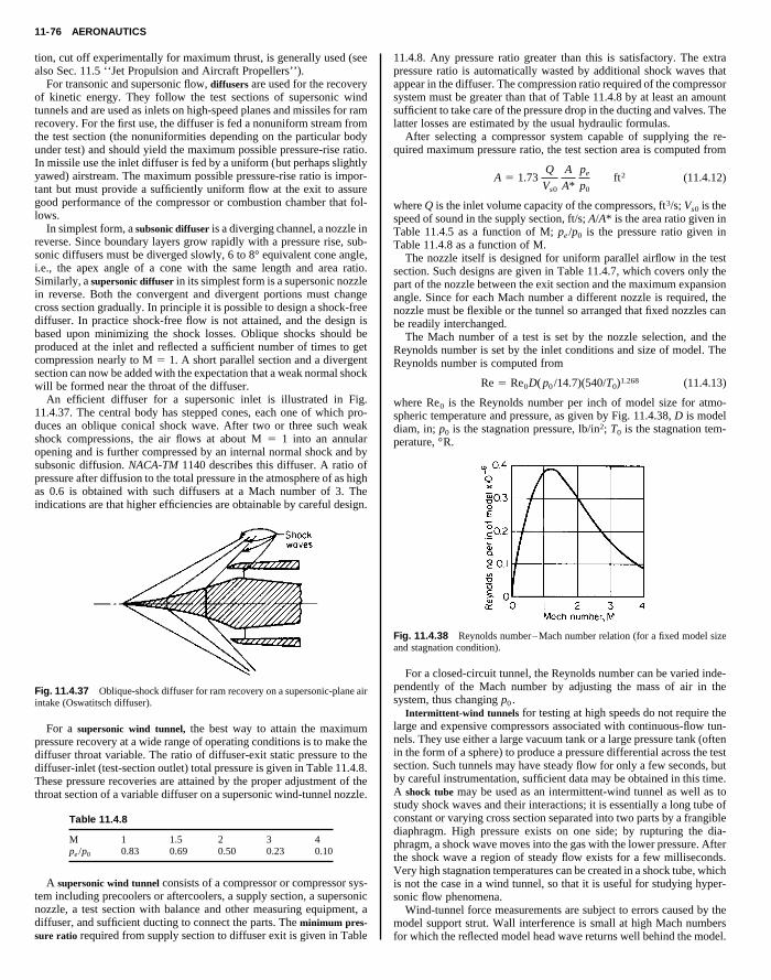
11-76 AERONAUTICS
tion, cut off experimentally for maximum thrust, is generally used (seealso Sec. 11.5 ‘‘Jet Propulsion and Aircraft Propellers’’).
For transonic and supersonic flow, diffusers are used for the recoveryof kinetic energy. They follow the test sections of supersonic windtunnels and are used as inlets on high-speed planes and missiles for ramrecovery. For the first use, the diffuser is fed a nonuniform stream fromthe test section (the nonuniformities depending on the particular bodyunder test) and should yield the maximum possible pressure-rise ratio.In missile use the inlet diffuser is fed by a uniform (but perhaps slightlyyawed) airstream. The maximum possible pressure-rise ratio is impor-
11.4.8. Any pressure ratio greater than this is satisfactory. The extrapressure ratio is automatically wasted by additional shock waves thatappear in the diffuser. The compression ratio required of the compressorsystem must be greater than that of Table 11.4.8 by at least an amountsufficient to take care of the pressure drop in the ducting and valves. Thelatter losses are estimated by the usual hydraulic formulas.
After selecting a compressor system capable of supplying the re-quired maximum pressure ratio, the test section area is computed from
A 5 1.73Q A pe ft2 (11.4.12)
Copyright (C) 1999 by The McGraw-Hill Companies, Inc. All rights reserved. Use ofthis product is subject to the terms of its License Agreement. Click here to view.
tant but must provide a sufficiently uniform flow at the exit to assuregood performance of the compressor or combustion chamber that fol-lows.
In simplest form, a subsonic diffuser is a diverging channel, a nozzle inreverse. Since boundary layers grow rapidly with a pressure rise, sub-sonic diffusers must be diverged slowly, 6 to 8° equivalent cone angle,i.e., the apex angle of a cone with the same length and area ratio.Similarly, a supersonic diffuser in its simplest form is a supersonic nozzlein reverse. Both the convergent and divergent portions must changecross section gradually. In principle it is possible to design a shock-freediffuser. In practice shock-free flow is not attained, and the design isbased upon minimizing the shock losses. Oblique shocks should beproduced at the inlet and reflected a sufficient number of times to getcompression nearly to M 5 1. A short parallel section and a divergentsection can now be added with the expectation that a weak normal shockwill be formed near the throat of the diffuser.
An efficient diffuser for a supersonic inlet is illustrated in Fig.11.4.37. The central body has stepped cones, each one of which pro-duces an oblique conical shock wave. After two or three such weakshock compressions, the air flows at about M 5 1 into an annularopening and is further compressed by an internal normal shock and bysubsonic diffusion. NACA-TM 1140 describes this diffuser. A ratio ofpressure after diffusion to the total pressure in the atmosphere of as highas 0.6 is obtained with such diffusers at a Mach number of 3. Theindications are that higher efficiencies are obtainable by careful design.
Fig. 11.4.37 Oblique-shock diffuser for ram recovery on a supersonic-plane airintake (Oswatitsch diffuser).
For a supersonic wind tunnel, the best way to attain the maximumpressure recovery at a wide range of operating conditions is to make thediffuser throat variable. The ratio of diffuser-exit static pressure to thediffuser-inlet (test-section outlet) total pressure is given in Table 11.4.8.These pressure recoveries are attained by the proper adjustment of thethroat section of a variable diffuser on a supersonic wind-tunnel nozzle.
Table 11.4.8
M 1 1.5 2 3 4pe /p0 0.83 0.69 0.50 0.23 0.10
A supersonic wind tunnel consists of a compressor or compressor sys-tem including precoolers or aftercoolers, a supply section, a supersonicnozzle, a test section with balance and other measuring equipment, adiffuser, and sufficient ducting to connect the parts. The minimum pres-sure ratio required from supply section to diffuser exit is given in Table
Vs0 A* p0
where Q is the inlet volume capacity of the compressors, ft3/s; Vs0 is thespeed of sound in the supply section, ft/s; A/A* is the area ratio given inTable 11.4.5 as a function of M; pe /p0 is the pressure ratio given inTable 11.4.8 as a function of M.
The nozzle itself is designed for uniform parallel airflow in the testsection. Such designs are given in Table 11.4.7, which covers only thepart of the nozzle between the exit section and the maximum expansionangle. Since for each Mach number a different nozzle is required, thenozzle must be flexible or the tunnel so arranged that fixed nozzles canbe readily interchanged.
The Mach number of a test is set by the nozzle selection, and theReynolds number is set by the inlet conditions and size of model. TheReynolds number is computed from
Re 5 Re0D( p0 /14.7)(540/T0)1.268 (11.4.13)
where Re0 is the Reynolds number per inch of model size for atmo-spheric temperature and pressure, as given by Fig. 11.4.38, D is modeldiam, in; p0 is the stagnation pressure, lb/in2; T0 is the stagnation tem-perature, °R.
Fig. 11.4.38 Reynolds number–Mach number relation (for a fixed model sizeand stagnation condition).
For a closed-circuit tunnel, the Reynolds number can be varied inde-pendently of the Mach number by adjusting the mass of air in thesystem, thus changing p0 .
Intermittent-wind tunnels for testing at high speeds do not require thelarge and expensive compressors associated with continuous-flow tun-nels. They use either a large vacuum tank or a large pressure tank (oftenin the form of a sphere) to produce a pressure differential across the testsection. Such tunnels may have steady flow for only a few seconds, butby careful instrumentation, sufficient data may be obtained in this time.A shock tube may be used as an intermittent-wind tunnel as well as tostudy shock waves and their interactions; it is essentially a long tube ofconstant or varying cross section separated into two parts by a frangiblediaphragm. High pressure exists on one side; by rupturing the dia-phragm, a shock wave moves into the gas with the lower pressure. Afterthe shock wave a region of steady flow exists for a few milliseconds.Very high stagnation temperatures can be created in a shock tube, whichis not the case in a wind tunnel, so that it is useful for studying hyper-sonic flow phenomena.
Wind-tunnel force measurements are subject to errors caused by themodel support strut. Wall interference is small at high Mach numbersfor which the reflected model head wave returns well behind the model.

LINEARIZED SMALL-DISTURBANCE THEORY 11-77
Near M 5 1, the wall interference becomes very large. In fact, thetunnel chokes at Mach numbers given in Table 11.4.5, at
A
A*5
1
1 2area of model projected on test-section cross section
area of test-section cross sectionarea of test-section cross section(11.4.14)
There are two choking points: one subsonic and one supersonic. Be-tween these two Mach numbers, it is impossible to test in the tunnel. Asthese Mach numbers are approached, the tunnel wall interference be-
ciated increase of drag and, often, flow separation at the base of theshock.
The redistribution of pressures and the motion of shock waves overthe wing surfaces through the transonic regime demands special consid-eration in the design of control surfaces so that they do not becomeineffective by separation or inoperative by excessive loading.
If a body is slender (i.e., planes tangent to its surface at any pointmake small angles with the flight direction), the disturbance velocitiescaused by this body will be small compared with the flight speed and,excluding the hypersonic regime, small compared with the speed of
Copyright (C) 1999 by The McGraw-Hill Companies, Inc. All rights reserved. Use ofthis product is subject to the terms of its License Agreement. Click here to view.
comes very large.For tests in this range of Mach number, specially constructed tran-
sonic wind tunnels with perforated or slotted walls have been built. Theobject here is to produce a mean flow velocity through the walls thatcomes close to that which would have existed there had the body beenmoving at that speed in the open. Often auxiliary blowers are needed toproduce the necessary suction on the walls and to reinject this air intothe tunnel circuit in or after the diffuser section.
Drag is difficult to predict precisely from wind-tunnel measurements,especially in the transonic regime. Flight tests of rocket-boosted modelswhich coast through the range of Mach numbers of interest are used toobtain better drag estimates; from telemetered data and radar or opticalsighting the deceleration can be determined, which in turn yields thedrag.
LINEARIZED SMALL-DISTURBANCE THEORY
As the speed of a body is increased from a low subsonic value (Fig.11.4.39a), the local Mach number becomes unity somewhere in thefluid along the surface of the body, i.e., the lower critical Mach numberis reached. Above this there is a small range of transonic speed in whicha supersonic region exists (Fig. 11.4.39b). Shock waves appear in thisregion attached to the sides of the body (Fig. 11.4.39c) and grow withincreasing speed. At still higher transonic speeds a detached shock waveappears ahead of the body, and the earlier side shocks either disappearor move to the rear (Fig. 11.4.39d). Finally, for a sharp-nosed body, thehead wave moves back and becomes attached (Fig. 11.4.39e). The flowis now generally supersonic everywhere, and the transonic regime isreplaced by the supersonic regime. With the appearance of shock wavesthere occurs a considerable alteration of the pressure distribution, andthe center of pressure on airfoil sections moves from the one-fourthchord point back toward the one-half chord point. There is an asso-
Fig. 11.4.39 Regions of flow about an airfoil (Mach numbers are approximate).
sound. This permits the use of linearized small-disturbance theory topredict the approximate flow past the body. This theory relates thesteady flow past the body at subsonic speeds to the incompressible flowpast a distorted version of this body (the ‘‘generalized Prandtl-Glauertrule’’). To find the velocity components in the subsonic flow about anyslender body, first determine the velocity components, u, v, w (in the x,y, z directions, respectively), in the incompressible flow, at the samestream speed, about a stretched shape whose streamwise (x-axis direc-tion) dimensions are 1/b times as great (b 5 √1 2 M2). The desiredvelocity components are then b2 2u, b2 1v, b2 1w at correspondingpoints of the stretched and unstretched bodies. For thin airfoil sectionsthis theory predicts
CL 5 2pa/ √1 2 M2 a in radians (11.4.15)
where L 5 CLqS and q 5 (g/2)p0M2. For finite-span wings and forbodies, no such simple relations exist. However, an approximation tothe overall lift coefficient for thin flat wings of rectangular platform is(see Fig. 11.4.41):
CL 5 2pAa/[2 1 √4 1 (bA)2] (11.4.16)
and the drag is made up of the induced drag due to lift and the skin-fric-tion drag (see above, ‘‘Airfoils’’).
CD 5 (CL /pA)(1 1 0.01bA) 1 CDF (11.4.17)
At supersonic speeds, the Prandtl-Glauert rule is also applicable if wereplace b by l 5 √M2 2 1 and relate flow to flow past a stretched (orcompressed) body at M 5 √2, where l 5 1. For thin airflow sections (seeFig. 11.4.40) this theory predicts
CL 5 4a/ √M2 2 1 a in radians (11.4.18)
CD 52
lE1
0FSdyu
dxD2
1Sdyl
dxD2G dSx
cD 14a2
l1 CDF
(11.4.19)
where dyu /dx and dyl /dx are the slopes of the upper and lower surfacesof the airfoil, respectively, and CDF is again the skin-friction drag coef-ficient. Note that there is a drag due to thickness and a drag due to lift atsupersonic speeds for an airfoil section where there is none at subsonicspeeds. For symmetric double-wedge airfoil sections, the thickness dragcoefficient becomes (4/l)(t/c)2, and for symmetric biconvex airfoil sec-tions it is (16/3l)(t/c)2, where t is the maximum thickness.
y
ay,(x)
yu(x)
V1
c
x
t
Fig. 11.4.40 Supersonic airfoil section.
Within the acoustic approximation, a disturbance at a point in super-sonic flow can affect only the points in the downstream Mach cone, i.e., aconical region with apex at the point, axis parallel to the stream direc-tion, and semicone angle equal to the Mach angle (see Fig. 11.4.32).Thus a rectangular wing with constant airfoil section has two-dimen-sional flow on all parts of the wing except the points within the tip Mach

11-78 AERONAUTICS
Fig. 11.4.41 Lift-coefficient curve slope for rectangular and delta wings (according to linearized theory).
Fig. 11.4.42 Drag due to lift for rectangular and delta wings (according to linearized theory).
cones. At Mach numbers near unity these tip Mach cones cover nearlythe entire wing, whereas at high Mach numbers they cover only a smallpart. Figure 11.4.41 shows the lift-curve coefficient slope for flatrectangular and delta plan-form wings at subsonic and supersonic speeds;these predictions of acoustic theory are inaccurate for high-aspect-ratiowings in the transonic regime, but elsewhere compare favorably withexperiment. Figure 11.4.42 shows the drag due to lift for the samewings. The reduction in drag due to lift of the delta wing relative to therectangular wing at moderate supersonic speeds, predicted by acoustictheory and shown in Fig. 11.4.42, is due to the fact that the delta-wing
Copyright (C) 1999 by The McGraw-Hill Companies, Inc. All rights reserved. Use ofthis product is subject to the terms of its License Agreement. Click here to view.
leading edge is swept back, and the component of velocity normal to theleading edge is subsonic. This creates a leading-edge suction whichreduces the drag. This drag reduction is only partially realized in prac-tice; a wing with a rounded leading edge realizes more of this reductionthan a wing with a sharp leading edge. Figure 11.4.43 shows the thick-ness drag of the rectangular and delta wings, which occurs only atsupersonic speeds. Note again that the leading-edge sweepback of thedelta wing helps to reduce this drag at moderate supersonic speeds.
The lift of a slender axially symmetric body at small angle of attack isnearly independent of Mach number and is given approximately by
CL 5 2a (11.4.20)
where the lift coefficient is based on the cross-sectional area of the base.The drag for a 5 0 at subsonic speeds is made up of skin friction and
Fig. 11.4.43 Supersonic thickness drag coefficient for rectangular and deltawings with a symmetrical double-wedge airfoil section (according to linearizedtheory).

LINEARIZED SMALL-DISTURBANCE THEORY 11-79
base drag; a dead-air region exists just behind the blunt base, and thepressure here is below ambient, causing a rearward suction which is thebase drag. At supersonic speeds a wave drag is added, which representsthe energy dissipated in shock waves from the nose. Figure 11.4.44shows a typical drag-coefficient curve for a body of revolution wherethe fineness ratio (ratio of length to diameter) is 12.2. The skin-frictiondrag coefficient based on wetted area is the same as that of a flat plate,within experimental error.
Cf
Copyright (C) 1999 by The McGraw-Hill Companies, Inc. All rights reserved. Use ofthis product is subject to the terms of its License Agreement. Click here to view.
Fig. 11.4.44 Drag coefficients for parabolic-arc (NACA-RM 10) body (calcula-tions from experimental data for a 30,000-ft altitude, D 5 12 in, from NACR-TR1160 and 1161, 1954).
At transonic and moderate supersonic speeds, the wave drag of a wingbody combination can be effectively reduced by making the cross-sec-tional area distribution (including wings) a smooth curve when plottedversus fuselage station. This is the area rule; its application results in adecided indentation in the fuselage contour at the wing juncture. Liftinterference effects also occur, especially when the body diameter is notsmall compared with the wing span. If the wing is attached to a cylin-drical body, and if the wing-alone lift coefficient would have been CL ,then the lift carried on the body is KBCL , and the lift carried on the wingis KWCL . Figure 11.4.45 shows the variation of KB and KW with bodydiameter to wing-span ratio.
Fig. 11.4.45 Wing-body lift-interface factors.
The effect of compressibility on skin-friction drag is slight at subsonicspeeds, but at supersonic speeds, a significant reduction in skin-frictioncoefficient occurs. Figure 11.4.46 shows the turbulent-boundary-layermean skin-friction coefficient for a cone as a function of wall tempera-ture and Mach number. An important effect at high speed is aerodynamicheating.
Figure 11.4.47 illustrates the velocity profile behind the shock waveof a body traveling at hypersonic speed. The shock-wave front repre-
Fig. 11.4.46 Laminar skin-friction coefficient for a cone.
sents an area of high-temperature gas which radiates energy to the body,but boundary-layer convective heating is usually the major contributor.Behind this front is shown the velocity gradient in the boundary layer.The decrease in velocity in the boundary layer is brought about by theforces of interaction between fluid particles and the body (viscosity).This change in velocity is accompanied by a change in temperature andis dependent on the characteristics of the boundary layer. For example,heat transfer from a turbulent boundary layer may be of an order ofmagnitude greater than for laminar flow.
Fig. 11.4.47 Velocity profile behind a shock wave.
If the gas is brought to rest instantaneously, the total energy in theflow is converted to heat and the temperature of the air will rise. Theresulting temperature is known as the stagnation temperature (see stag-nation point, Fig. 11.4.47).
TS 5 T` S1 1g 2 1
2M2D (11.4.21)
T` is the ambient temperature of the gas at infinity, and g is thespecific-heat ratio of the gas. For undissociated air, g 5 1.4.
In general, this simple, one-dimensional relationship between veloc-ity and temperature does not hold for temperature in the boundary layer.The laminae of the boundary layer are not insulated from each other,and there is cross conduction. This is associated with the Prandtl numberPr, which is defined as
Pr 5 Cp m/kr (11.4.22)
where kr 5 thermal conductivity of fluid, Cp 5 specific heat of fluid atconstant pressure, and m 5 absolute viscosity of fluid.
Defining the recovery factor r as the ratio of the rise in the idealisticwall and stagnation temperature over the free-stream temperature,
r 5 (Taw 2 T`)/(Ts 2 T`) 5 (Pr)n (11.4.23)

11-80 AERONAUTICS
For laminar flow, r 5 (Pr)1/2; and for turbulent flow, r 5 (Pr)1/3.Prandtl number Pr greatly complicates the thermal computations, but
since it varies only over a small range of values, a recovery factor of0.85 is generally used for laminar flow and 0.90 for turbulent flow.
where Cp 5 specific heat of air; Cf 5 local skin-friction coefficient;r0 5 density outside of boundary layer; V 5 velocity outside of bound-ary layer; g 5 acceleration of gravity.
For a cone, kr 5 1,800 (laminar Re , 2 3 106) and kr 5 1,800r4/3
(turbulent).For a flat-plate transition, Reynolds number is 1 3 106.Figure 11.4.46 gives laminar-skin-friction coefficient for a cone. For
a flat plate, multiply Cf by √3/2. For turbulent skin-friction coefficientfor a cone,
0.242
Copyright (C) 1999 by The McGraw-Hill Companies, Inc. All rights reserved. Use ofthis product is subject to the terms of its License Agreement. Click here to view.
Fig. 11.4.48 Variation of stagnation and adiabatic wall temperature with Machnumber.
For a thermally thin wall, the rate of change of the surface tempera-ture is a function of the rate of total heat input and the surface’s ability toabsorb the heat.
dTw /dt 5 qT /wcb (11.4.24)
where t 5 time, qT 5 forced convective heating 1 radiation heating 2heat radiation from the skin, w 5 density of skin material, c 5 specificheat of skin material, b 5 skin thickness, and Tw 5 skin temperature.
The heat balance may then be written
wcb SdTw
dt D 5 kcFT0S1 1 rgB 2 1
2M2
0D 2 TwG1 aGsAp 2 esT 4
w (11.4.25)
where Ap 5 correction factor to account for area normal to radiationsource, gB 5 specific heat ratio of boundary layer, e 5 radiativeemissivity of surface, s 5 Stefan-Boltzmann constant [17.3 3 10210
Btu/(h ? ft2 ?°R4), a 5 surface absorptivity, Gs 5 solar irradiation Btu/(h ? ft2).
For small time increments D t,
dTw
dt5
Tw2 2 Tw1
Dt
Then
Tw2 5 Tw1 1Dt
wcb HhcFT0S1 1gB 2 1
2M2
0D 2 TwG1 aGsAp 2 T 4
wJ (11.4.26)
The local heat-transfer coefficient hc is defined as
hc 5kr
r4/3CpCfr0Vg (11.4.27)
Fig. 11.4.49 Stagnation-temperature probe (recovery factor 5 0.98).
√A2CfTw /T0
(sin21 c 1 sin21 u)
5 0.41 logRe
2Cf 2 1.26 log
Tw
T0
(11.4.28)
where
c 52A2 2 B
√B2 1 4A2A2 5
(g0 2 1⁄2)M20
Tw /T0
u 5B
√B2 1 4A2B 5
1 1 (g0 2 1⁄2)M20
Tw /T0
2 1
For a flat plate, use Re instead of Re/2 in Eq. (11.4.28).Figure 11.4.48 shows data on stagnation and adiabatic wall tempera-
tures.The primary measurements in aerodynamics are pressure measure-
ments. A well-aligned pitot tube with an impact-pressure hole at its noseand static-pressure holes 10 diameters or more back from the nose willaccurately measure the impact pressure and the static pressure of a uni-form gas stream. Up to sonic speed the impact pressure is identical withstagnation pressure, but at supersonic speeds, a detached shock waveforms ahead of the probe, through which there is drop in stagnationpressure; the portion of the shock wave just ahead of the probe is nor-mal, so that the equation for water flow in layer form over horizontaltubes (see ‘‘Transmission of Heat by Conduction and Convection’’ inSec. 4) gives the relation of the measured impact pressure to the isen-tropic stagnation pressure.
Force measurements of total lift, drag, side force, pitching moment,yawing moment, and rolling moment on models are made on wind-
Condensing lens
Mirror
Mirror MirrorKnife edgecutoff
Photo plate
Camera
Camera
Wind tunnel
Optical flat
Arc light sourceCondensing lens
Source knife edgeWind tunnel
Wind tunnel
Light source
(a)
(b)
(c)
Light source
Optical flat
Splitter plateSplitterplate
Monochromatic filter
Mirror
Fig. 11.4.50 Optical systems for observing high-speed flow phenomena.(a) Interferometer; (b) Schlieren (two-mirror) system; (c) shadowgraph.

JET PROPULSION AND AIRCRAFT PROPELLERS 11-81
tunnel balances just as at low speed. Small internal-strain-gage balancesare often used to minimize strut interference.
An open thermocouple is unreliable for determining stagnation tem-perature if it is in a stream of high velocity. Figure 11.4.49 shows asimple temperature probe in which the fluid is decelerated adiabaticallybefore its temperature is measured. The recovery factor used in equa-tions, for this probe, accurately aligned to the stream, is 0.98.
Optical measurements in high-speed flow depend on the variation ofindex of refraction with gas density. This variation is given by
where k 5 0.116 ft3/slug for air. A Mach-Zehnder interferometer (Fig.11.4.50a), is capable of giving accurate density information for two-dimensional and axially symmetric flows. The Schlieren optical system(Fig. 11.4.50b) is sensitive to density gradients and is the most com-monly used system to determine location of shock waves and regions ofcompression or expansion. The shadowgraph optical system is the sim-plest system (Fig. 11.4.50c) and is sensitive to the second space deriva-tive of the density.
Drd
equivalent to an actuator disk, which imparts only an axial accelerationto the air flowing through it. The rotation of the actuator disk produces a
Copyright (C) 1999 by The McGraw-Hill Companies, Inc. All rights reserved. Use ofthis product is subject to the terms of its License Agreement. Click here to view.
n 5 1 1 kr (11.4.29)
11.5 JET PROPULSION ANby Sanfo
REFERENCES: Zucrow, ‘‘Aircraft and Missile Propulsion,’’ Vol. 2, Wiley. Hilland Peterson, ‘‘Mechanics and Thermodynamics of Propulsion,’’ Addison-Wes-
ley. Sutton, ‘‘Rocket Propulsion Elements,’’ Wiley. Shorr and Zaehringer, ‘‘SolidPropellant Technology,’’ Wiley. Forestor and Kuskevics, ‘‘Ion Propulsion,’’AIAA Selected Reprints. Theodorsen, ‘‘Theory of Propellers,’’ McGraw-Hill.Smith, ‘‘Propellers for High Speed Flight,’’ Princeton. Zucrow, ‘‘Principles of JetPropulsion,’’ Wiley. ‘‘Aircraft Propeller Handbook,’’ Depts. of the Air Force,Navy, and Commerce, U.S.‘‘Aircraft Engines and Gas Tudynamics of Aircraft Gas Tu‘‘Aeroelasticity for TurbomacAIRCRAFT PROPELLERSFleeter
slipstream composed of the entire mass of air flowing in the axial direc-tion through the area of the actuator disk, i.e., the circle swept by thepropeller. Atmospheric air enters the slipstream with the flight speed V0
and mass flow rate ma. It leaves the slipstream with the wake velocity w.n systems utilizing pro-
or detailed discussions offt Propellers.’’)
Government Printing Office, 1956. Kerrebrock,rbines,’’ MIT Press. Oates, ed., ‘‘The Aerothermo-rbine Engines,’’ AFAPL-TR-78-52, 1978. Fleeter,hine Applications,’’ AIAA J. of Aircraft, 16, no. 5,
The thrust is given in Eq. (11.5.5). Propulsiopellers will be termed propeller propulsion. (Fthe airplane propeller, see the section ‘‘Aircra
1979. Bathie, ‘‘Fundamentals of Gas Turbines,’’ Wiley. Hagar and Vrabel, ‘‘Ad-vanced Turboprop Project,’’ NASA SP 495, 1988. ‘‘Aeronautical Technologies forthe Twenty-First Century,’’ National Academy Press. Mattingly, Heiser, andDaley, ‘‘Aircraft Engine Design,’’ AIAA.
Newton’s reaction principle, based on the second and third laws ofmotion, is the theoretical basis for all methods of propelling a bodyeither in (or on) a fluid medium or in space. Thus, the aircraft propeller,the ships screw, and the jet propulsion of aircraft, missiles, and boats areall examples of the application of the reaction principle to the propul-sion of vehicles. Furthermore, all jet engines belong to that class ofpower plants known as reaction engines.
Newton’s second law states that a change in motion is proportional tothe force applied; i.e. a force proportional to the rate of change of thevelocity results whenever a mass is accelerated: F 5 ma. This can beexpressed in a more convenient form as F 5 d(mv)/dt, which makes itclear that the application of the reaction principle involves the time rateof increase of the momentum (mv) of the body. It should be noted thatthe same force results from either providing a small acceleration to alarge mass or a large acceleration to a small mass.
Newton’s third law defines the fundamental principle underlying allmeans of propulsion. It states that for every force acting on a body thereis an equal and opposite reaction force.
The application of this reaction principle for propulsion involves theindirect effect of increasing the momentum of a mass of fluid in onedirection and then utilizing the reaction force for propulsion of thevehicle in the opposite direction. Thus, the reaction to the time rate ofincrease of the momentum of that fluid, called the propulsive fluid,creates a force, termed the thrust, which acts in the direction of motiondesired for the propelled vehicle. The known devices for achieving thepropulsion of bodies differ only in the methods and mechanisms forachieving the time rate of increase in the momentum of the propulsivefluid or matter.
The function of a propeller is to convert the power output of anengine into useful thrust. To do this it accelerates a mass of air in thedirection opposite to the direction of flight, generating thrust via New-ton’s reaction principle. Figure 11.5.1 illustrates schematically, in therelative coordinate system for steady flow, the operating principle of theideal aircraft propeller. Power is supplied to the propeller, assumed to be
Fig. 11.5.1 Ideal propeller in the relative coordinate system.
Jet propulsion differs from propeller propulsion in that the propulsivefluid (or matter), instead of being caused to flow around the propelledbody, is ejected from within the propelled body in the form of one ormore high-speed jets of fluid or particles. In fact, the jet propulsionengine is basically designed to accelerate a large stream of fluid (ormatter) and to expel it at a high velocity. There are a number of ways ofaccomplishing this, but in all instances the resultant reaction or thrustexerted on the engine is proportional to the time rate of increase of themomentum of the fluid. Thus, jet engines produce thrust in an analo-gous manner to the propeller and engine combination. While the pro-peller gives a small acceleration to a large mass of air, the jet enginegives a larger acceleration to a smaller mass of air.
Theoretically, there are no restrictions on either the type of matter,called the propellant, for forming a high-velocity jet or the means forproducing the propulsive jet. The selection of the most suitable propel-lant and the most appropriate jet propulsion engine is dictated by thespecific mission for the propelled vehicle. For example, in the case ofthe jet propulsion of a boat, termed hydraulic jet propulsion, the propul-sive jet is formed from the water on which the boat moves. For thepractical propulsion of bodies through either the atmosphere or in space,however, only two types of propulsive jets are suitable:
1. For propulsion within the atmosphere, there is the jet formed byexpanding a highly heated, compressed gas containing atmospheric airas either a major or a sole constituent. Such an engine is called either an

11-82 JET PROPULSION AND AIRCRAFT PROPELLERS
airbreathing or a thermal-jet engine. If the heating is accomplished byburning a fuel in the air, the engine is a chemical thermal-jet engine. If theair is heated by direct or indirect heat exchange with a nuclear-energysource, the engine is termed a nuclear thermal-jet engine.
2. For propulsion both within and beyond the atmosphere of earth,there is the exhaust jet containing no atmospheric air. Such an exhaustjet is termed a rocket jet, and any matter used for creating the jet is calleda propellant. A rocket may consist of a stream of gases, solids, liquids,ions, electrons, or a plasma. The assembly of all the equipment requiredfor producing the rocket jet constitutes a rocket engine.
diffuser the air is further diffused so that it arrives at the entrance to thecombustion chamber with the required low Mach number. If P0 is thetotal pressure of the free-stream air having the Mach number M0 and P2
that for the air entering the combustion system with the Mach numberM2 , then it is desirable that P2 /P0 be a maximum.
In the combustion chamber a fuel is burned in the air, thereby raisingthe total temperature of the gases entering the exhaust nozzle (see Sec.7) to approximately T7 5 4260°R (2366 K). Most generally a liquidhydrocarbon fuel is used, but experiments have been conducted withsolid fuels, liquid hydrogen, liquid methane, and ‘‘slurries’’ of metallic
Copyright (C) 1999 by The McGraw-Hill Companies, Inc. All rights reserved. Use ofthis product is subject to the terms of its License Agreement. Click here to view.
Modern airbreathing engines may be segregated into two principaltypes: (1) ramjet engines, and (2) turbojet engines. The turbojet enginesare of two types: (1) the simple turbojet engine, and (2) the turbofan, orbypass, engine.
Rocket engines can be classified by the form of energy used forachieving the desired jet velocity. The three principal types of rocketengines are (1) chemical rocket engines, (2) nuclear heat-transfer rocketengines, and (3) electric rocket engines.
The propulsive element of a jet-propulsion engine, irrespective oftype, is the exhaust nozzle or orifice. If the exhaust jet is gaseous, theassembly comprising all the other components of the jet-propulsionengine constitutes a gas generator for supplying highly heated, high-pressure gases to the exhaust nozzle.
These classifications of jet-propulsion engines apply to the basictypes of engines. It is possible to have combinations of the differenttypes of thermal-jet engines and also combinations of thermal-jet en-gines with rocket engines; only the principal types are discussed here.
ESSENTIAL FEATURES OF AIRBREATHING ORTHERMAL-JET ENGINES
In the subsequent discussions a relative coordinate system is employedwherein the atmospheric air flows toward the propulsion system withthe flight speed V0, and the gases leave the propulsion system with thevelocity w, relative to the walls of the propulsion system. Furthermore,steady-state operating conditions are assumed.
Ramjet Engine Figure 11.5.2 illustrates schematically the essentialfeatures of the simple ramjet engine. It comprises three major compo-nents: a diffusion or inlet system, (0–2); a combustion chamber (2–7);and an exhaust nozzle (7–9). In this simple ramjet engine, apart fromthe necessary control devices, there are no moving parts. However, foraccelerating the vehicle or for operating at different Mach numbers, avariable geometry diffuser and exhaust may be required.
Fig. 11.5.2 Ramjet engine.
The operating principle of the ramjet engine is as follows. The free-stream air flowing toward the engine with a velocity V0 and Machnumber M0 is decelerated by the inlet diffuser system so that it arrives atthe entrance to the combustion chamber with a low Mach number, onthe order of M2 5 0.2. When the inlet-flow Mach number is supersonic,this diffuser system consists of a supersonic diffuser followed by asubsonic diffuser. The supersonic diffuser decelerates the inlet flow toapproximately unity Mach numbers at the entrance to the subsonic dif-fuser; this deceleration is accompanied by the formation of shock wavesand by an increase in the pressure of the air (diffusion). In the subsonic
fuels in a liquid fuel. The combustion process is not quite isobaricbecause of the pressure drops in the combustion chamber, because ofthe increase in the momentum of the working fluid due to heat addition,and because of friction. The hot gases are discharged to the atmo-sphere, after expanding in the exhaust nozzle, with the relative velocityw 5 V9 .
Since the ramjet engine can function only if there is a ram pressurerise at the entrance to the combustion chamber, it is not self-operating atzero flight speed. It must, therefore, be accelerated to a flight speedwhich permits the engine to develop sufficient thrust for acceleratingthe vehicle it propels to the design flight Mach number. Consequently, aramjet-propelled missile, for example, must either be launched by drop-ping it from an airplane or be boosted to the required flight speed bymeans of launching, or bootster, rockets. It appears that the most appro-priate flight regime for the ramjet is at low to moderate supersonic Machnumbers, between approximately M0 5 2 and 5. The lower limit isassociated with the necessary ram pressure rise while the upper limit isset by the problem of either cooling or protecting the outer skin of theengine body.
Scramjet Low-cost access to space is one of the major reasons forthe interest in hypersonic propulsion (speeds above Mach 5). A vehicle toprovide access to space must be capable of reaching very high Machnumbers, since orbital velocity (17,000 mi/h) is about Mach 24. Theramjet engine, which must slow the entering air to a low subsonic ve-locity, cannot be used much above Mach 5 or 6. The solution is todecelerate the flow in the engine to a supersonic Mach number lowerthan the flight Mach number but greater than the local speed of sound.This propulsion device is the supersonic combustion ramjet, or scramjet,which is capable, in principle, of operation to Mach 24. As shownschematically in Fig. 11.5.3, in contrast to the ramjet, the scramjet en-
Fig. 11.5.3 Ramjet and scramjet flow configurations.

ESSENTIAL FEATURES OF AIRBREATHING OR THERMAL-JET ENGINES 11-83
gine requires that fuel be added to the air, mixed, and burned, all atsupersonic velocities, which is a significant technical challenge.
The advantage derived from supersonic combustion of the liquid fuel(usually liquid hydrogen) is that the diffuser of the scramjet engine isrequired to decelerate the air entering the engine from M0 to only ap-proximately M2 5 0.35 M0 instead of the M2 5 0.2, which is essentialwith subsonic combustion. This elimination of the subsonic diffusionincreases the diffuser efficiency, reduces the static pressure in the com-bustor (and, therefore, the engine weight and heat transfer rate), andincreases the velocity in the combustor (thereby decreasing engine
The thrust of the simple turbojet engine increases rapidly with T4 ,because increasing T4 increases the jet velocity Vj . Actually, Vj in-creases faster than the corresponding increase in T4 . It is also an inher-ent characteristic of the gas-turbine engine which produces shaft power,called a turboshaft engine, that its useful power increases proportionallyfaster than a corresponding increase in its turbine inlet temperature T4 .Because of the decrease in strength of turbine materials with increase intemperature, the turbine blades, stators, and disks require cooling atT4 . 2160°R (1200 K) approximately. T4 values are currently in the2860 to 3260°R (1589 to 1811 K) range, and are being pushed toward
Copyright (C) 1999 by The McGraw-Hill Companies, Inc. All rights reserved. Use ofthis product is subject to the terms of its License Agreement. Click here to view.
frontal area). It is the combination of the above effects that makesramjet propulsion at high flight Mach numbers (. 7) feasible.
Pulsejets may be started and operated at considerably lower speedsthan ramjets. A pulsejet is a ramjet with an air inlet which is providedwith a set of shutters loaded to remain in the closed position. After thepulsejet engine is launched, ram air pressure forces the shutters to open,fuel is injected into the combustion chamber, and is burned. As soon asthe pressure in the combustion chamber equals the ram air pressure, theshutters close. The gases produced by combustion are forced out the jetnozzle by the pressure that has built up within the chamber. When thepressure in the combustion chamber falls off, the shutters open again,admitting more air, and the cycle repeats at a high rate.
Simple Turbojet Engine Figure 11.5.4 illustrates schematically theprincipal features of a simple turbojet engine, which is basically a gas-turbine engine equipped with a propulsive nozzle and diffuser. Atmo-spheric air enters the engine and is partially compressed in the diffusionsystem, and further compressed to a much higher pressure by the aircompressor, which may be of either the axial-flow or centrifugal type.The highly compressed air then flows to a combustion chamber whereinsufficient fuel is burned to raise the total temperature of the gases enter-ing the turbine to approximately T4 5 2160°R (1200 K) for an uncooledturbine. The maximum allowable value for T4 is limited by metallur-gical and stress considerations; it is desirable, however, that T4 be ashigh as possible. The combustion process is approximately isobaric.The highly heated air, containing approximately 25 percent of combus-tion products, expands in the turbine, which is directly connected to theair compressor, and in so doing furnishes the power for driving the aircompressor. From the turbine the gases pass through a tailpipe whichmay be equipped with an afterburner. The gases are expanded in asuitably shaped exhaust nozzle and ejected to the atmosphere in theform of a high-speed jet.
Fig. 11.5.4 Simple turbojet engine.
Like the ramjet engine, the turbojet engine is a continuous-flow en-gine. It has an advantage over the ramjet engine in that its functioningdoes not depend upon the ram pressure of the entering air, although theamount of ram pressure recovered does affect its overall economy andperformance. The turbojet is the only airbreathing jet engine that hasbeen utilized as the sole propulsion means for piloted aircraft. It appearsto be eminently suited for propelling aircraft at speeds above 500 mi/h(805 km/h). As the design flight speed is increased, the ram pressureincreases rapidly, and the characteristics of the turbojet engine tend tochange over to those of the ramjet engine. Consequently, its top speedappears to be limited to that flight speed where it becomes more advan-tageous to employ the ramjet engine. It appears that for speeds aboveapproximately 2,000 mi/h (3,219 km/h) it is advantageous to use someform of a ramjet engine.
the 4,600°R (2556 K) stoichiometric limit of JP4 fuel. The cooling air isbled from the compressor at the appropriate stage (or stages) and used tocool the stator blades or rotor blades by convective, film, or transpira-tion heat transfer. Up to 10 percent of the compressor air may be bledfor turbine cooling, and this air is ‘‘lost’’ for turbine work for that bladerow where it is used for cooling. Consequently ‘‘trade’’ studies must bemade to ‘‘weigh’’ the increased complexity of the engine and the tur-bine work loss due to air bleed against the increased engine perfor-mance associated with increased T4 .
As in the case of any gas-turbine power plant, the efficiencies of thecomponents of the turbojet engine have an influence on its performancecharacteristics, but its performance is not nearly as sensitive to changesin the efficiency of its component machines as is a gas turbine whichdelivers shaft power. (See Sec. 9.)
As noted previously, two types of compressors are currently em-ployed, the axial-flow compressor and the centrifugal compressor. Irre-spective of the type, the objectives are similar. The compressor must bereliable, compact, easy to manufacture, and have a small frontal area.Because of the limited air induction capacity of the centrifugal com-pressor, also called the radial compressor, engines for developingthrusts above 7,000 lb (31 kN) at static sea level employ axial-flowcompressors (see Sec. 14).
The turbojet engine exhibits a rather flat thrust-versus-speed curve.Because the ratio of the takeoff thrust to thrust in flight is small, certainoperational problems exist at takeoff. Since the exhaust gases from theturbine contain considerable excess air, the jet velocity, and conse-quently the thrust, can be increased by burning additional fuel in thetailpipe upstream from the exhaust nozzle. By employing ‘‘tailpipeburning,’’ or ‘‘afterburning,’’ as it is called, the thrust can be increasedby 35 percent and at 500 mi/h, in a tactical emergency, by approxi-mately 60 percent. With afterburning, the temperature of the gases en-tering the nozzle T7 , is of the order of 3800°R (2110 K).
Turbofan, or Bypass, Engine For a fixed turbine inlet temperature,the jet velocity from a simple turbojet engine propelling an airplane atsubsonic speed is relatively constant. The propulsive efficiency dependson the ratio of the flight speed to the jet velocity and increases as theratio increases. On the other hand, the thrust depends on the differencebetween the jet velocity and the flight speed; the larger the difference,the larger the thrust per unit mass of air induced into the engine. Byreducing the jet velocity and simultaneously increasing the mass rate ofairflow through the engine, the propulsive efficiency can be increasedwithout decreasing the thrust. To accomplish this, a turbofan or bypassengine is required.
Figure 11.5.5 illustrates schematically the components of a turbofanengine. There are two turbines, a low-pressure turbine (LPT) and ahigh-pressure turbine (HPT); one drives the air compressor of the hot-gas generator and the other drives the fan. Air enters the fan at the rate of~maF and is ejected through the nozzle of area A7F with the jet velocity
VjF , Vj , where Vj is the jet velocity attained by the air flowing throughthe hot-gas generator with the mass flow rate ~ma1 ; the hot-gas generatoris basically a turbojet engine.
A key parameter is the bypass ratio, defined as the ratio of the air massflow rate through the fan bypass duct to that through the hot-gas genera-tor ( ~maF / ~ma1). Bypass ratios of about 5 to 10 are in use, with values ofabout 5 utilized in modern large commercial transport engines, for ex-ample, the Pratt & Whitney 4000 and the General Electric CF-6. Thehot-gas generator is basically a turbojet engine. The fuel is added to ~ma1
at the rate ~mf . The hot-gas stream ( ~ma1 1 ~mf ) is discharged to the

11-84 JET PROPULSION AND AIRCRAFT PROPELLERS
atmosphere through A7 with the velocity Vj . Both types of turbofanengine produce an ‘‘overall’’ jet velocity VjTF which is smaller than thatfor a turbojet engine operating with the same P3 /P2 and T4 . The ar-rangements shown in Fig. 11.5.5 are for subsonic propulsion. Fuel can,of course, be burned in the fan air maF for increasing the thrusts of the
The next generation of large transport engines will be conventionalhigh-bypass engines, but will have a larger thrust capability and willoffer further improvements in specific fuel consumption, achieved byusing even higher overall pressure ratios (over 40 : 1) and turbine inlettemperature (over 1850 K or 2870°F) combined with even more effi-cient components (Fig. 11.5.6). Beyond these conventional high-bypassengines, will be the ultrahigh-bypass-ratio engine in either a ducted oropen rotor form (Fig. 11.5.7). The ducted ultrahigh-bypass-ratio enginefeatures a counterrotating, reversible-pitch fan powered by a gearedcore engine with an overall 80 : 1 cycle pressure ratio. It is likely to be
Copyright (C) 1999 by The McGraw-Hill Companies, Inc. All rights reserved. Use ofthis product is subject to the terms of its License Agreement. Click here to view.
Fig. 11.5.5 Two different schematic arrangements of components of turbofanengines (subsonic flight). (a) Aft-fan turbofan engine; (b) ducted-fan turbofanengine.
engines. Practically all the newer commercial passenger aircraft arepropelled by turbofan engines, and most of the older jet aircraft havebeen refurbished with new turbofan engines. The advantage of thelower effective jet velocity VjTF is twofold: (1) It increases the propul-sive efficiency hp by reducing v 5 VjTF /V0 and, consequently, raises thevalue of h0 . (2) The reduced jet velocity reduces the jet noise; the latterincreases with approximately the eighth power of the jet speed.
Fig. 11.5.6 Efficiency trends.
used on the larger aircraft, since it does not restrain the aircraft configu-ration or flight speed and will provide a 35 percent improvement in fuelburned over the most advanced current subsonic high-bypass engines.
Fig. 11.5.7 Ultrahigh-bypass-ratio engine configurations.
A highly loaded, multiblade swept variable-pitch propeller, the prop-fan or advanced turboprop, could be combined with the latest turbineengine technology. The resulting advanced turboprop would offer apotential fuel saving of 50 percent over an equivalent-technology turbo-fan engine operating at competitive speeds and altitudes because of theturboprop’s much higher installed efficiency. To eliminate the gearboxdevelopment for a 20,000 shaft horsepower engine, the propfans of theunducted fan (UDF) engine were directly driven with counterrotatingturbine stages, a unique concept (Fig. 11.5.8). The projected specific
Fig. 11.5.8 UDF counterrotating turbine configuration.
fuel consumption at cruise for the resulting gearless, counterrotatingUDF engine was 30 percent lower than that of the most modern turbofanengines, and about 50 percent lower than that of engines presently in useon 150-passenger airplanes. The tremendous fuel-saving potential of theturboprop has already been demonstrated. If economic conditionschange, this concept could replace conventional high-bypass-ratio tur-bofans on small aircraft and military transports.

ESSENTIAL FEATURES OF ROCKET ENGINES 11-85
ESSENTIAL FEATURES OF ROCKET ENGINES
Figure 11.5.9 is a block-type diagram illustrating the essential featuresof a rocket engine, which comprises three main components: (A) asupply of propellant material contained in the rocket-propelled vehicle,(B) a propellant feed and metering system, and (C) a thrust chamber,also called a rocket motor, thrustor, or accelerator. In any rocket engine,energy must be added to the propellant as it flows through the thrustor.
Except in those cases where the operating duration of the rocketmotor is very short or where the combustion temperature is low, meansmust be provided for protecting the interior walls of the motor. The twomost common methods are ablative cooling and regenerative cooling. Inablative cooling the inner surfaces of the thrust chamber are covered withan ablative material which vaporizes, thereby providing some cooling.Ordinarily, the material leaves a ‘‘char’’ which acts as a high-tempera-ture insulating material. For high-performance engines which are tooperate for relatively long periods, regenerative cooling is employed. Inregenerative cooling, one of the propellants is circulated around the walls
Copyright (C) 1999 by The McGraw-Hill Companies, Inc. All rights reserved. Use ofthis product is subject to the terms of its License Agreement. Click here to view.
Fig. 11.5.9 Essential features of a rocket engine.
In Figure 11.5.9 propellant material from the supply is metered and fedto the thrust chamber, where energy is added to it. As a consequence ofthe energy addition, the propellant is discharged from the thrustor withthe jet velocity Vj . The thrustor F acts in the direction opposite to thatfor the jet velocity Vj .
Chemical Rocket Engines
All chemical rocket engines have two common characteristics: (1) Theyutilize chemical reactions in a thrust chamber to produce a high-pres-sure, high-temperature gas at the entrance to a converging-divergingexhaust nozzle; (2) the hot propellant gas expands in flowing throughthe exhaust nozzle, and the expansion process converts a portion of thethermal energy, released by the chemical reaction, into the kinetic en-ergy associated with a high-velocity gaseous-exhaust jet. Chemicalrocket engines may be grouped into (1) liquid-bipropellant rocket en-gines, (2) liquid-monopropellant rocket engines, and (3) solid-propel-lant rocket engines.
Liquid-Bipropellant Rocket Engine Figure 11.5.10 illustrates theessential features of a liquid-bipropellant rocket engine employing tur-bopumps for feeding two propellants, an oxidizer and a fuel, to a rocketmotor. The motor comprises (1) an injector, (2) a combustion chamber,and (3) a converging-diverging exhaust nozzle. The liquid propellantsare fed under pressure, through the injector, into the combustionchamber, where they react chemically to produce large volumes of
Fig. 11.5.10 Essential features of a liquid-bipropellant rocket engine.
high-temperature, high-pressure gases. For a given propellant combina-tion, the combustion temperature Tc depends primarily on the oxidizer-fuel ratio (by weight), termed the mixture ratio, and to a lesser extentupon the combustion static pressure pc . When the mass rate of flow ofthe liquid propellants equals that of the exhaust gases, the combustionpressure remains constant—the mode of operation that is usually de-sired.
If the bipropellants react chemically when their liquid streams comein contact with each other, they are said to be hypergolic. Propellantswhich are not hypergolic are said to be diergolic, and some form ofignition system is required to initiate combustion.
before injection into the motor. In some engines the regenerative cool-ing is combined with local liquid film cooling at critical areas of thethrust chamber. See Table 11.5.1 for bipropellant combinations.
Refer to Figure 11.5.10. By removing the oxidizer tank, the oxidizerpump, and the plumbing associated with the liquid oxidizer, one obtainsthe essential elements of a liquid-monopropellant rocket engine. Suchan engine does not require a liquid oxidizer to cause the monopropellantto decompose and release its thermochemical energy.
There are basically three groups of monopropellants: (1) liquidswhich contain the fuel and oxidizer in the same molecule, e.g., hydro-gen peroxide (H2O2) or nitromethane (CH3NO2); (2) liquids whichcontain either the oxidizer or the fuel constituent in an unstable molecu-lar arrangement, e.g., hydrazine (N2H4); and (3) synthetic mixtures ofliquid fuels and oxidizers. The most important liquid monopropellantsare hydrazine and hydrogen peroxide (up to 98% H2O2). Hydrazine canbe decomposed by a suitable metal catalyst, which is ordinarily packedin a portion of the thrust chamber at the injector end. The decompositionof hydrazine yields gases at a temperature of 2260°R (1265 K); thegases are a mixture of hydrogen and ammonia. Hydrogen peroxide canbe readily decomposed either thermally, chemically, or catalytically.The most favored method is catalytically; a series of silver screenscoated with samarium oxide is tightly packed in a decompositionchamber located at the injector end of the thrust chamber. At Pc 5 300psia, the decomposition of hydrogen peroxide (98%) yields gases hav-ing a temperature of 2260°R (1256 K).
The specific impulse obtainable for a liquid monopropellant is con-siderably smaller than that obtainable from liquid-bipropellant systems.Consequently, monopropellants are used for such auxiliary purposes asthrust vernier control, attitude reaction controls for space vehicles andmissiles, and for gas generation.
Solid-propellant Rocket Engine Figure 11.5.11 illustrates sche-matically a solid-propellant rocket engine employing an internal-burn-ing case-bonded grain; the latter burns radially outward at a substantially
Fig. 11.5.11 Essential features of an internal-burning case-bonded solid-propellant rocket engine.
constant rate. A solid propellant contains both its fuel and the requisiteoxidizer. If the fuel and oxidizer are contained in the molecules formingthe solid propellant, the propellant is termed a double-base propellant.Those solid propellants wherein a solid fuel and a solid oxidizer form anintimate mechanical mixture are termed either composite or heteroge-neous solid propellants. The chemical reaction of a solid propellant is

11-86 JET PROPULSION AND AIRCRAFT PROPELLERS
Table 11.5.1 Calculated Values of Specific Impulse for Liquid Bipropellent Systemsa
[Pc 5 1,000 lbf/in2 (6,896 3 103 N/m2) to Pe 5 1 atm]Shifting equilibrium; isentropic expansion; adiabatic combustion; one-dimensional flow
Temperature Tc
Oxidizer Fuel ~mo / ~mf r °R K c* I (s)
Chlorine trifluoride (CTF) Hydrazine 2.80 1.50 6553 3640 5961 293.1(ClF3) MMHb 2.70 1.41 5858 3254 5670 286.0
Pentaborane (B5H9) 7.05 1.47 7466 4148 5724 289.0
Fluorine (F2) Ammonia 3.30 1.12 7797 4332 7183 359.5Hydrazine 2.30 1.31 8004 4447 7257 364.0Hydrogen 7.70 0.45 6902 3834 8380 411.1Methane 4.32 1.02 7000 3889 6652 343.8RP-1 2.62 1.21 6839 3799 6153 318.0
Hydrogen peroxide Hydrazine 2.00 1.26 4814 2674 5765 287.4(100% H2O2) MMH 3.44 1.26 4928 2738 5665 284.8
IRFNAc Hydined 3.17 1.26 5198 2888 5367 270.3MMH 2.57 1.24 5192 2885 5749 275.5
Nitrogen tetroxide Hydrazine 1.30 1.22 5406 3002 5871 292.2(N2O4) Aerozine-50e 2.00 1.21 5610 3117 5740 289.2
MMH 2.15 1.20 5653 3141 5730 288.7
Oxygen (LOX) (O2) Hydrazine 0.91 1.07 5667 3148 6208 312.8Hydrogen 4.00 0.28 4910 2728 7892 291.2Methane 3.35 0.82 6002 3333 6080 310.8Pentaborane 2.21 0.91 7136 3964 6194 318.1RP-1 2.60 1.02 6164 3424 5895 300.0
a Based on ‘‘Theoretical Performance of Rocket Propellant Combinations,’’ Rocketdyne Corporation, Canoga Park, CA.b MMH: Monomethyl hydrazine (N2H3CH3).c IRFNA: Inhibited red fuming nitric acid; 84.4% (HNO3), 14% (N2O4), 1% (H2O), 0.6% (HF).d Hydine: 60% UDMH f, 40% Deta g.e Aerozine-50: 50% UDMH f, 50% hydrazine (N2H4).f UDMII: Unsymmetrical dimethylhydrazine (CH3)2N2H4.g DETA: Diethylenetriamine (C2H13N3).
initiated by an igniter. In general, the configuration of a propellant graincan be designed so that the area of the burning surface of the propellantvaries to give a prescribed thrust-versus-time curve.
Nuclear Heat-transfer Rocket Engine
Figure 11.5.12 illustrates schematically a nuclear heat-transfer rocketengine employing a solid-core reactor. The heat generated by the fissionsof the uranium nucleus is utilized for heating a gaseous propellant, suchas hydrogen, to a high temperature of 4000°R (2200 K) approx at theentrance section of the exhaust nozzle. The hot gas is ejected to the
The propellant in a nuclear heat-transfer rocket engine functions ba-sically as a fluid for cooling the solid-core nuclear reactor. Its reaction isnot based on energy considerations alone, but on such properties asspecific heat, latent heat, molecular weight, and liquid density and oncertain practical considerations.
Electric Rocket Engines
Several different types of electric rocket engines have been conceived;the principal types are described below. All of them require some formof power plant for generating electricity. Thus the power plant may be
Copyright (C) 1999 by The McGraw-Hill Companies, Inc. All rights reserved. Use ofthis product is subject to the terms of its License Agreement. Click here to view.
surroundings after expansion in a converging-diverging exhaust nozzle.The basic difference between the operating principles of a nuclear heat-transfer and a chemical rocket engine is the substitution of nuclearfission for chemical reaction as the source of heat for the propellant gas.Since the exhaust nozzle is the propulsive element, the remaining com-ponents of the nuclear heat-transfer rocket engine constitute the hot-gasgenerator.
Fig. 11.5.12 Schematic arrangement of a nuclear heat-transfer rocket engine.
nuclear, solar-cell batteries, thermoelectric, or other. The choice of thetype of power plant depends upon the characteristics of both the electricrocket engine and the space-flight mission. Figure 11.5.13 illustratesdiagrammatically an electric rocket engine, comprising (1) a nuclearpower source, (2) an energy-conversion unit for obtaining the desiredform of electric energy, (3) a propellant feed and metering system,(4) an electrically operated thrustor, and (5) the requisite control de-vices. Electric rocket engines may be classified as (1) electrothermal,(2) electromagnetic, and (3) electrostatic.
Fig. 11.5.13 Essential features of an electric rocket engine.

ESSENTIAL FEATURES OF ROCKET ENGINES 11-87
Electrothermal Rocket Engine Figure 11.5.14a illustrates the typeof engine which uses electric power for heating gaseous propellant to ahigh temperature before ejecting it through a converging-diverging ex-haust nozzle. If an electric arc is employed for heating the propellant,the engine is called a thermal arc-jet rocket engine.
Electromagnetic Rocket Engine Figure 11.5.14b illustrates anelectromagnetic, or plasma, rocket engine. There is a wide variety ofsuch engines, but all of them utilize the same operating principle. Aplasma (a neutral ionized conducting gas) is accelerated by means of itsinteraction with either a stationary or a varying magnetic field. Basi-
electric rocket engine is placed in an earth orbit, the low-thrust electricrocket engine, under the conditions in space, will accelerate it to a largevehicle velocity if the operating time for the engine is sufficiently long.
In a chemical rocket engine, the energy for propulsion, as well as themass ejected through the exhaust nozzle, is provided by the propellants,but the energy which can be added to a unit mass of the propellant gas isa fixed quantity, limited by the nature of the chemical bonds of thereacting materials. For that reason, chemical rocket engines are said tobe energy-limited rocket engines. Although a nuclear heat-transfer rocketengine is also energy-limited, the limitation is imposed by the amount of
Copyright (C) 1999 by The McGraw-Hill Companies, Inc. All rights reserved. Use ofthis product is subject to the terms of its License Agreement. Click here to view.
cally, a plasma engine differs from a conventional electric motor by thesubstitution of a conducting plasma for a moving armature.
Electrostatic Rocket Engine Figure 11.5.14c illustrates schemati-cally the electrostatic, or ion, rocket engine, comprising (1) an electricpower plant; (2) a propellant supply; (3) ionization apparatus; (4) an ionaccelerator; and (5) an electron emitter for neutralizing the ion beamejected from the accelerator. Its operating principle is based on utilizingelectrostatic fields for accelerating and ejecting electrically chargedparticles with extremely large velocities. The overall objective is totransform thermal energy into the kinetic energy associated with anextremely high-velocity stream of electrically neutral particles ejectedfrom one or more thrustors. Mercury ion engines are currently beingtested. The engine provides thrust by a rapid, controlled discharge ofions created by the ionization of atoms of the mercury fuel supply. Solarcells convert sunlight into electricity, which is then used to bombard themercury with free electrons. This causes one electron to be strippedfrom each mercury atom, resulting in ionized mercury atoms. The ionsmix with other electrons to form a plasma. A magnetic field set upbetween two metal screens at the aft end of the engine draws the posi-tively charged ions from the plasma and accelerates them at very highexit speeds out the back of the engine. This creates a high-velocity exitbeam producing low-level but extremely long-term thrust.
Fig. 11.5.14 Electric rocket engine. (a) Electrothermal rocket engine. (b) elec-tromagnetic rocket engine. (c) electrostatic (ion) engine.
All electric rocket engines are low-thrust devices. The interest in suchengines stems from the fact that chemical-rocket technology, for exam-ple, the space shuttle, is now so advanced that it has become feasible toplace heavy payloads, such as a satellite equipped with an electricrocket engine, into an earth orbit. An electric rocket engine which isvirtually inoperable terrestrially can be positioned in space and can thenoperate effectively because of the absence of aerodynamic drag andstrong gravitational fields. Consequently, if a vehicle equipped with an
energy that can be added per unit mass of propellant without exceedingthe maximum allowable temperature for the materials employed for thesolid-core reactor.
In an electric rocket engine, on the other hand, the energy added tothe propellant is furnished by an electric power plant. The power avail-able for heating the propellant is limited by the maximum power outputof the electric power plant, accordingly, electric rocket engines arepower-limited.
Notation
a 5 acoustic speeda0 5 acoustic speed in free-stream aira2 5 burning rate constant for solid propellantAe 5 cross-sectional area of exit section of exhaust nozzleAp 5 area of burning surface for solid propellantAt 5 cross-sectional area of throat of exhaust nozzlecp 5 specific heat at constant pressurecv 5 specific heat at constant volumec* 5 PcAt / ~m 5 characteristic velocity for rocket motorCd 5 discharge coefficient for exhaust nozzleCF 5 thrust coefficient
CFg 5 gross-thrust coefficient for ramjet engineCFn 5 net thrust coefficient
D or $ 5 dragDi 5 ~maV0 5 ram drag for airbreathing or thermal-jet engined 5 diameter
dp 5 diameter of propellerEin 5 rate at which energy is supplied to propulsion systemEf 5 calorific value of fuelEp 5 calorific value of rocket propellants
f 5 ~mf / ~ma 5 fuel-air ratiof 9 5 f /hB 5 fuel-air ratio for ideal combustion chamberF 5 force or thrustFi 5 mew 2 miV0 1 ( pe 2 p0)Ae 5 thrust due to internal flowFj 5 meVj 5 jet thrustFp 5 ( pe 2 p0)Ae 5 pressure thrustFg 5 Fi 5 gross thrust for ramjet engine
FgSFC 5 gross-thrust specific-fuel consumption for ramjet enginegc 5 correction factor defined by Newton’s second law of
motionh 5 static specific enthalpy
Dhn 5 enthalpy change for exhaust nozzleH 5 total (stagnation) specific enthalpy
DHc 5 lower heating value of fuelI 5 specific impulse
Ia 5 F/gma 5 air specific impulseJ 5 mechanical equivalent of heat; advance ratio, propellerk 5 cp /cv 5 specific heat ratio
L or + 5 liftM 5 massm 5 mass rate of flow~ma 5 mass rate of air consumption for thermal-jet engine~me 5 mass rate of flow of gas leaving propulsion system~mf 5 mass rate of fuel consumption~mi 5 mass rate of flow of gas into propulsion system~mo 5 mass rate of oxidizer consumption for rocket engine~mp 5 ~mo 1 ~mf 5 mass rate of propellant consumption for rocket
engine

11-88 JET PROPULSION AND AIRCRAFT PROPELLERS
m 5 molecular weightMe 5 momentum of gases leaving propulsion system in unit timeMi 5 momentum of gases entering propulsion system in unit
timeM0 5 V0 /a0 5 Mach number of free-stream air (flight speed)
n 5 revolutions per unit timep 5 absolute static pressure; pitch of propeller blade
pc 5 absolute static pressure of gases in combustion chamberpe 5 absolute static pressure in exit section of exhaust nozzlep0 5 absolute static pressure of free-stream ambient air
hp 5 3T /(3T 1 3L ) 5 ideal propulsive efficiencyht 5 (T4 2 T5)/(T4 2 T95) 5 isentropic efficiency of turbine
h th 5 3/Ein 5 thermal efficiency of propulsion engine
l 5 gIa / √2gJcpt0 5 thrust parameter for turbojet engine; 1⁄2 1 1⁄2cos f 5 divergence coefficient for exhaust nozzle for rocketengines
n 5 V0 /w 5 speed ratior 5 densityr 5 mean density
2 (k 2 1)/(2k 2 1)
Copyright (C) 1999 by The McGraw-Hill Companies, Inc. All rights reserved. Use ofthis product is subject to the terms of its License Agreement. Click here to view.
P 5 absolute total (stagnation) pressurePc 5 absolute total pressure at entrance to exhaust nozzle
P0 5 p0S1 1k 2 1
2M2
0Dk/(k21)
5 absolute total pressure of
free-stream air3 5 propulsion power
3L 5 leaving loss3T 5 thrust power
q 5 rV 2/2 5 dynamic pressureq0 5 r0V 2
0 /2 5 k0 p0M20/2 5 dynamic pressure of free-stream air
Q 5 torqueQi 5 heat supplied to actual combustorQ9i 5 heat supplied to ideal combustor (no losses)r0 5 linear burning rate for solid propellantR 5 Ru /m 5 gas constant
Ru 5 universal gas constant 5 mRt 5 absolute static temperature
tp 5 temperature of solid propellant prior to ignitionT 5 absolute total (stagnation) temperature
Tc 5 absolute total temperature of gas entering exhaust nozzle ofrocket motor
T2 5 absolute total temperature at entrance to air compressor (seeFig. 11.5.4)
T3 5 absolute total temperature at exit section of air compressor(see Fig. 11.5.4)
T 93 5 absolute total temperature at exit section of ideal compressor(see Fig. 11.5.4) operating between same pressure limits asactual compressor
T4 5 absolute total temperature at entrance to turbine (see Fig.11.5.4)
T5 5 absolute total temperature at exit from turbine (see Fig.11.5.4)
T 95 5 absolute total temperature at exit from ideal turbineu 5 pndp 5 propeller tip speedV 5 velocity
VF 5 forward speed of propellerVj 5 effective jet velocityV0 5 velocity of free-stream air (flight speed)w 5 velocity of exit gases relative to walls of exhaust nozzle or
velocity of air in ultimate wake of propeller~W 5 weight rate of flow
~Wo 5 weight rate of flow of oxidizer~Wp 5 weight rate of flow of propellants
Greek
a 5 T4 /t0 5 ada1 5 cycle temperature ratio; angle of attackad 5 T2 /t0 5 diffusion temperature ratioa1 5 T4 /T2
b 5 bypass ratio for turbofans; helix angle for propeller bladed 5 P/Pstd corrected pressureh 5 efficiency
hB 5 f 9/f 5 efficiency of combustion for thermal-jet enginehc 5 (T93 2 T2)/(T3 2 T2) 5 isentropic efficiency of compressorhd 5 isentropic efficiency of diffuserhn 5 w2 5 isentropic efficiency of exhaust nozzleho 5 3T /Ein 5 overall efficiency of propulsion system
V 5 √kSk 1 1
Dv 5 angular velocity of propeller shaft
v9 5 rate of rotation of slipstream at propellerv99 5 rate of rotation of slipstream in ultimate slipstream
F 5 fan velocity coefficient 5 VF /uf 5 semiangle of exhaust-nozzle divergence; effective helix
angle
w 5 √hn 5 velocity coefficient for exhaust nozzler 5 densitys 5 solidity of propellerU 5 (P3 /p0)(k 2 1)/k 5 UdUc 5 cycle pressure ratio parameter
Uc 5 (P3 /P2)(k 2 1)/k 5 compressor pressure-ratio parameterUd 5 (P2 /p0)(k 2 1)/k 5 diffuser pressure-ratio parameterUn 5 (P7 /p0)(k 2 1)/k 5 (P7 /p9)(k 2 1)/k 5 nozzle pressure-ratio pa-
rameterUt 5 (P4 /P5)(k 2 1)/k 5 turbine pressure-ratio parameteru 5 T/Tstd 5 corrected temperature
Subscripts
(a) numbered0 5 free stream1 5 entrance to subsonic diffuser2 5 exit from subsonic diffuser3 5 entrance to combustion chamber4 5 entrance to turbine of turbojet engine5 5 exit from turbine of turbojet engine6 5 tail-pipe entrance7 5 entrance to exhaust nozzle8 5 throat section of exhaust nozzle9 5 exit section of exhaust nozzle
(b) lettereda 5 airB 5 burner or combustion chamberb 5 bladec 5 compressord 5 diffusere 5 exit section; effectiveF 5 fanf 5 fuelh 5 hydraulicn 5 nozzleo 5 overall or oxidizerp 5 propellantP 5 propulsive
std 5 standardt 5 turbine or throat, as specified in text
Statement on Units The dynamic equation employed in the fol-lowing sections are written for consistent sets of units, i.e., for sets inwhich 1 unit of force 5 1 unit of mass 3 1 unit of acceleration. Conse-quently, the gravitational correction factor gc in Newton’s equationF 5 (1/gc )ma (see notation) has the numerical value unity and is omit-ted from the dynamic equations. When the equations are used for calcu-lation purposes, gc should be included and its appropriate value em-ployed.

POWER AND EFFICIENCY RELATIONSHIPS 11-89
THRUST EQUATIONS FORJET-PROPULSION ENGINES
Refer to Fig. 11.5.15, which illustrates schematically a rotationallysymmetrical arbitrary propulsion engine immersed in a uniform flowfield. Because of the reactions between the fluid flowing through theengine, called the internal flow, and the interior surfaces wetted by theinternal flow a resultant axial force is produced, that is, a force collinearwith the longitudinal axis of the engine. If an axial force acts in theforward direction, employing a relative coordinate system, it is called athrust; if it acts in the backward direction it is called a drag. Similarly, the
where n 5 V0 /Vj .In the case of rocket engines, since they do not consume atmospheric
air, ~ma 5 0, and the flow of gas out of the rocket motor, under steady-state conditions, is equal to ~mp 2 ~mo 1 ~mf (see notation).
The effective jet velocity Vj is larger than Ve 5 exit velocity if pe . p0 ;that is, if the gases are underexpanded. The effective jet velocity is auseful criterion because it can be determined accurately from the mea-sured values of Fi and ~mp obtained from a static firing test of the rocketmotor.
The ratio Fi / ~mp is denoted by I and called either the specific thrust or
Copyright (C) 1999 by The McGraw-Hill Companies, Inc. All rights reserved. Use ofthis product is subject to the terms of its License Agreement. Click here to view.
resultant axial force due to the external flow, the flow passing over theexternal surfaces of the propulsion system, is a thrust or drag dependingupon whether it acts in the forward direction or the backward direction.
Fig. 11.5.15 Generalized jet-propulsion system.
Application of the momentum equation of fluid mechanics to thegeneralized propulsion system illustrated in Fig. 11.5.15 gives the fol-lowing equation for the thrust Fi due to the internal flow. Thus, if it isassumed that the external flow is frictionless, there is no change in therate of momentum for the external flow between Si and Se . Hence, thethrust F 5 Fi is due entirely to the internal flow, and
F 5 Fi 5 mew 2 ~miV0 1 ( pe 2 p0)Ae (11.5.1)
In Eq. (11.5.1), ~mew 5 Fj 5 jet thrust, ~miV0 5 Di 5 ram drag, and( pe 2 p0)Ae 5 Fp 5 pressure thrust. Hence,
Fi 5 Fj 2 Di 1 Fp (11.5.2)
It is convenient to introduce a fictitious effective jet velocity Vj , which isdefined by
F 5 ~meVj 2 ~miV0 5 ~mew 2 ~miV0 1 ( pe 2 p0)Ae (11.5.3)
If the gases are expanded completely, in the exhaust nozzle, then w 5 Vj
and Fp 5 0. No appreciable error is introduced, in general, if it isassumed that Fp 5 0. For thermal jet engines, ~mi 5 ~ma (see notation), and~me 5 ~ma 1 ~mf . Let f 5 ~mf / ~ma , v 5 V0 /Vj ; then
Fi 5S1 1 f
n2 1D ~maV0 1 ( pe 2 p0)Ae (11.5.4)
In the case of uncooled turbojet engines, ~mf is not significantly differ-ent from the fraction of ~ma utilized for cooling the bearings and turbinedisk. Consequently, no significant error is introduced by assuming that~me 5 ~ma 1 ~mf ' ~ma 5 ~m. Hence, for a simple turbojet engine, one may
write
Fe 5 ~ma(Vj 2 V0) 5 ~mV0(1/n 2 1) (11.5.5)
Equation (11.5.5) is also the thrust equation for an ideal propeller; inthat case Vj is the wake velocity for the air leaving its slipstream. Thetrust equation for a hydraulic jet propulsion system has the same form asEq. (11.5.5). Let V0 denote the speed of a boat, and ~mw the mass rate offlow of the water entering the hydraulic pump and discharged by theexit nozzle with the velocity w 5 Vj relative to the boat. Hence, forhydraulic jet propulsion
F 5 ~ms(Vj 2 V0) 5 ~mwV0(1/n 2 1) (11.5.6)
the specific impulse. Hence
I 5 F/ ~mp 5 Vj /gc (11.5.7)
Although the dimensions of specific impulse are force/(mass)(s), it isconventional to state its units as seconds.
Equation (11.5.5) for the thrust of a turbojet engine, when expressed interms of the effective jet velocity Vj , becomes
F 5 ~ma(Vj 2 V0) (11.5.8)
POWER AND EFFICIENCY RELATIONSHIPS
In a jet-propulsion engine the propulsion element is the exhaust nozzle,and the rate at which energy is supplied to it is called the propulsionpower, denoted by 3. The rate at which the propulsion system doesuseful work is termed the thrust power 3T and is given by
3T 5 FV0 (11.5.9)
Assume that pe 5 p0 , and that the only energy loss in a propulsionsystem is the leaving loss 3L 5 ~m(Vj 2 V0)2/2, that is, the kinetic energyassociated with the jet gases discharged from the system; then the pro-pulsive power is given by
3 5 3L 1 3T (11.5.10)
The ideal propulsive efficiency is defined, in general, by
hP 5 3T /(3T 1 3L ) 5 thrust power/propulsion power (11.5.11)
For a turbojet engine and hydraulic jet propulsion,
hP 5 2n/(1 1 n) (11.5.12)
For a chemical rocket engine,
hP 5 2n/(2 1 n2) (11.5.13)
The propulsive efficiency hP is of more or less academic interest. Ofmore importance is the overall efficiency ho , which for airbreathing androcket engines is defined by
ho 5 hthhP (11.5.14)
where
hth 5 3/Ein 5 thermal efficiency of system (11.5.15)
and Ein is the rate at which energy is supplied to the propulsion system.The overall efficiency of a hydraulic jet-propulsion system is given
by
ho 5 hthhhhp 5 hhhth [2n/(1 1 n)] (11.5.16)
where hth is the thermal efficiency of the power plant which drives thewater pump, and hh is the hydraulic efficiency of the water pump. Toachieve a reasonable fuel consumption rate, hh must have a larger value.
For an airbreathing jet engine, Ein 5 ~mf (Ef 1 V 20 /2), and
ho 52n
1 1 n
3
~mf (Ef 1 V 20 /2)
(11.5.17)
The ratio ~mf /F is called the thrust specific-fuel consumption (TSFC)and is measured in mass of fuel per hour per unit of thrust. Hence,
TSFC 5 ~mf /F 5 f ~ma /F (11.5.18)

11-90 JET PROPULSION AND AIRCRAFT PROPELLERS
For a rocket engine, Ein 5 ~mp(Ep 1 V 20 /2), so that
ho 52n
1 1 n2
3
~mp(Ep 1 V20 /2)
(11.5.19)
PERFORMANCE CHARACTERISTICS OFAIRBREATHING JET ENGINES
The Ramjet Engine In ramjet technology the thrust due to the inter-nal flow Fi is called the gross thrust and denoted by Fg . Refer to Fig.
Total pressurePart of engine ratio
Supersonic diffuser (0–1) P1 /P0 5 0.92Subsonic diffuser (1–2) P2 /P1 5 0.90Flameholders (2–7) P7 /P2 5 0.97Combustion chamber (2–7) P7 /P2 5 0.92Exhaust nozzle (7–9) P9 /P7 5 0.97
The Simple Turbojet Engine A good insight into the design per-
Copyright (C) 1999 by The McGraw-Hill Companies, Inc. All rights reserved. Use ofthis product is subject to the terms of its License Agreement. Click here to view.
11.5.2 and assume ~m0 ' ~m9 5 ~ma . Then
Fg 5 Fi ' ~ma(Vj 2 V0) (11.5.20)
In level unaccelerated flight Fg is equal to the external drag of thepropelled vehicle and the ramjet body.
It is customary to express the thrust capabilities of the engine in termsof the gross-thrust coefficient CFg. If Am is the maximum cross-sectionalarea of the ramjet engine, q0 5 r0V 2
0 /2 5 k0 p0M20/2 5 the dynamic
pressure of the free-stream air, then
CFg 5Fg
q0Am
52Fg
Amk0 p0M20
(11.5.21)
In terms of the Mach numbers M0 and M9,
CFg 52A9 /Am
k0M20SP9
p0
1 1 k9M29
P9 /p9
2 1D 2 2A0
Am
(11.5.22)
In a fixed-geometry engine, M9 depends upon the total temperatureT7 , the total pressure P7 , the fuel-air ratio f, the nozzle area ratio Ae /At ,and the efficiency of the nozzle hn . For estimating purposes, k0 5 1.4and k9 5 1.28, when the engine burns a liquid-hydrocarbon fuel. Themanner in which CFg varies with altitude M0 and fuel-air ratio f is shownschematically in Fig. 11.5.16.
Fig. 11.5.16 Effect of altitude and fuel-air ratio on the gross-thrust coefficientof a fixed-geometry ramjet engine. (a) Effect of altitude; (b) effect of fuel-air ratio.
If a 5 T7/t0 5 cycle temperature ratio, and kB is the mean value ofk for the combustion gases, the rate at which heat is supplied to the en-gine is
Qi 5 Q9i /hB 5 ~macpBt0(a 2 T2)/hB (11.5.23)
It is readily shown that
Qi 5A0 p0V0
hBJ
kB
kB 2 1 Fa 2S1 1k0 2 1
2M2
0DG (11.5.24)
The gross-thrust specific-fuel consumption (FgSFC) is, by definition,
FgSFC 5 ~mf /Fg (11.5.25)
The principal sources of loss are aerothermodynamic in nature andcause a decrease in total pressure between stations 0 and 7. For estimat-ing purposes, assuming M0 5 2.0 and T6 5 3800°R (2111 K ), the totalpressures across different sections of the engine may be assumed to beapproximately those tabulated below.
formance characteristics of the turbojet engine is obtained convenientlyby making the following assumptions: (1) The mass rate of flow ofworking fluid is identical at all stations in the engine; (2) the thermody-namic properties of the working fluid are those for air; (3) the air is aperfect gas and its specific heats are constants; (4) there are no pressurelosses due to friction or heat addition; (5) the exhaust nozzle expandsthe working fluid completely so that p9 5 p0 ; and (6) the auxiliarypower requirements can be neglected. Refer to Fig. 11.5.4 and let
U 5SP3
p0D(k 2 1)/k
Ud 5SP2
p0D(k 2 1)/k
Uc 5SP3
P2D(k 2 1)/k
Ut 5SP4
P5D(k 2 1)/k
Un 5SP7
p0D(k 2 1)/k
5SP7
p9D(k 2 1)/k
a 5 T4 /t0 ad 5 T2 /t0 a1 5 T4 /T2
In view of the assumptions,
U 5 UdUc 5 UtUn (11.5.26)
and
a 5 aaa1 (11.5.27)
The diffuser pressure-ratio parameter Ud is given by
Ud 5 1 1 hd [(k 2 1)/2]M20 (11.5.28)
where hd 5 isentropic efficiency of diffuser (0.75 to 0.90 for well-designed systems).
The turbine pressure-ratio parameter Ut is given by
1/Ut 5 1 2 [(Uc 2 1)/a1hcht ] (11.5.29)
where ht 5 the isentropic efficiency of the turbine (0.90 to 0.95).Heat supplied, per unit mass of air, is
Q1 5 (cp /hB )(T4 2 T3)
or
Qi 5cpt0
hBhc
adS a
ad
hc 2 hc 2 Uc 1 1D (11.5.30)
where hc is the isentropic efficiency of the air compressor (0.85 to 0.90),and hB is the efficiency of the burner (0.95 to 0.99).
The enthalpy change for the exhaust nozzle Dhn is given by
Dhn
cpt0
5hn
hc
[ahc 2 ad (Uc 2 1)]
3H1 2a1hcht
Uc[1 1 hd(ad 2 1)][a1hcht 2 (Uc 2 1)]J (11.5.31)
The specific thrust, also called the air specific impulse, is
Ia 5 Fi / ~mag 5 (√2Dhn 2 V0)/ ~ma (11.5.32)
The overall efficiency ho is given by
ho 5 hthhp 5IaV0
JQi
5 2hBhc
lM0 Sk 2 1
2 D1/2
ahc 2S1 1k 2 1
2M2
0D(hc 1 Uc 2 1)
(11.5.33)

PERFORMANCE CHARACTERISTICS OF AIRBREATHING JET ENGINES 11-91
where hB ranges from 0.95 to 0.99 and l is the dimensionless turbojetspecific thrust parameter.
The TSFC for a turbojet engine is given by
TSFC 5~mf
F(11.5.34)
It can be shown by dimensional analysis, if the effects of Reynoldsnumbers are neglected, that the variables entering into the performanceof a given turbojet engine may be grouped as indicated in Table 11.5.2.
approximately equal to 19. Curve B applies to the design point of en-gines having a fixed compressor pressure ratio of 10 : 1 but havingdifferent values of a, that is, turbine inlet temperature. It shows thatincreasing a much above a 5 5 reduces the overall efficiency andconsequently TSFC. Curve C presents the design-point characteristicsfor engines operating with a 5 5 but having different compressor pres-sure ratios. The maximum value of l is obtained at a relatively lowpressure ratio: approximately P3 /P2 5 5. Curve D presents the design-point characteristics of engines having a fixed compressor pressure ratioof 10 : 1 but different cycle temperature ratios. Increasing a gives sig-
Copyright (C) 1999 by The McGraw-Hill Companies, Inc. All rights reserved. Use ofthis product is subject to the terms of its License Agreement. Click here to view.
Table 11.5.2
Nondimensional group Uncorrected form Corrected form
Flight speed V0 /√t0 V0 /√u
Rotational speed N /√T N /√u
Air flow rate ~Wa√T /D2P ~Wa√u/d
Thrust F /D2P F /d
Fuel flow rate ~Wf JDHc /D2P√T ~Wf /d√u
u 5 T /Tstd 5 T /519 (T /288) 5 corrected temperature (exact value for Tstd is 518.699°R).d 5 P /pstd 5 P /14.7 (P /1.013 3 105) 5 corrected pressure.
Figure 11.5.17 is a design-point chart presenting l and ho as func-tions of a, P3/P2 , and Uc for the subsonic performance of simple turbo-jet engines. The curves apply to propulsion at 30,000 ft. (9.14 km)altitude for engines having characteristic data indicated in the figure.Curve A illustrates the effect of pressure ratio P3/P2 or Uc for enginesoperating with a 5 5.0. It is seen that increasing the compressor pres-sure ratio increases ho but it approaches a maximum value at P3 /P2
Fig. 11.5.17 Dimensionless thrust parameter l and overall efficiency h0 asfunctions of the compressor pressure ratio (simple turbojet engine).
nificant increases in l. Hence, large values of turbine inlet temperatureT4 offer the potential for large thrusts per unit of frontal area for suchturbojet engines.
Figure 11.5.18 presents the design-point characteristics for engineshaving hc 5 0.85, ht 5 0.90, hr 5 0.93, and hB 5 0.99. Different valuesof diffuser efficiency are presented for flight Mach numbers M0 5 0.8(hd 5 0.91), M0 5 1.60 (hd 5 0.90) and M0 5 2.4 (hd 5 0.88). Twodifferent classes of engines are considered, those with P3 /P2 5 4.0 andthose with P3 /P2 5 12.0. The dimensionless thrust l is plotted as afunction of a with M0 as a parameter. It is evident that increasing l, thatis, the turbine inlet temperature T4 , offers the advantage of a largeincrease in thrust per unit area of the engine under all the conditionsconsidered in Fig. 11.5.18.
Figure 11.5.19 presents the effect of flight speed on the design-pointperformance, at 30,000 ft (9.14 km) altitude, for engines having hc 50.85, ht 5 0.90, hB 5 0.95, T4 5 2000°R (1111 K) and burning a fuelhaving a heating value DHc 5 18,700 Btu/ lbm (10,380 kcal /kgm). Themagnitude of the compressor pressure ratio P3 /P2 approaches unitywhen V0 is approximately 1,500 mi/h, indicating that at higher speedsthe compressor and turbine are superfluous; i.e., the propulsion require-ments would be met more adequately by a ramjet engine. Raising T4
tends to delay the aforementioned condition to a high value of V0 .
Fig. 11.5.18 Dimensionless thrust parameter l for a simple turbojet engine andits overall efficiency ho as functions of the cycle temperature ratio a, with theflight Mach number as a parameter.

11-92 JET PROPULSION AND AIRCRAFT PROPELLERS
It is a characteristic of turbojet engines, since ho 5 hthhp , that for agiven M0 increasing hth causes Dhn to increase, and hence the jet veloc-ity Vj . As a consequence, hp is decreased. It is this characteristic whichcauses ho 5 f (a), curve B of Fig. 11.5.17, to be rather flat for a widerange of values of a 5 T4 /t0 .
The curves of Figs. 11.5.17 to 11.5.19 are design-point performancecurves; each point on a curve is the design point for a different turbojetengine. The performance curves for a specific engine are either com-puted from experimental data pertaining to its components operatingover a wide range of conditions or obtained from testing the complete
Mechanical Design
Blades New technologies being developed to achieve higher thrust-to-weight ratios in advanced gas turbine engines also cause higher vi-bratory blade row responses and stresses that delay engine developmentand may adversely affect engine reliability. In particular, the designtrend toward higher stage loadings and higher specific flow are beingattained through increased tip speeds, lower radius ratios, lower aspectratios, and fewer stages. The resultant axial-flow compressor blade de-signs utilize thin, low-aspect-ratio blading with corresponding highsteady-state stresses. Also, the mechanical damping is considerably re-
Copyright (C) 1999 by The McGraw-Hill Companies, Inc. All rights reserved. Use ofthis product is subject to the terms of its License Agreement. Click here to view.
turbojet engine. It is customary to present the data in standardized form.
Fig. 11.5.19 TSFC and specific thrust Ia functions of the compressor pressureratio, with flight speed as a parameter (simple turbojet engine).
The Turbofan or the Ducted-Fan Engine Refer to Fig. 11.5.5b. As-sume that the hot-gas flow ( ~ma1 1 ~mf ) is ejected through the convergingnozzle, area At , with the effective jet velocity Vj , and that the airflow~maF is ejected through the converging annular nozzle, area A7F , with the
jet velocity VjF . Let b 5 ~maF / ~ma1 denote the bypass ratio, approxi-mately 5 for modern transport engines.
The thrust equation for the turbofan engine is
F 5 ~ma1(1 1 f )Vj 1 b ~ma1VjF 2 ~ma1(1 1 b)V0 (11.5.35)
where VjF , Vj . The thrust per unit mass of airflow, or air specificimpulse, is
Ia 5 F/ ~ma1(1 1 b) (11.5.36)
The TSFC is given by
TSFC 5 ~mf /F (11.5.37)
One of the most important applications of turbofans is for high-sub-sonic transport aircraft where the fuel consumption in cruise is a majorconsideration. In general, as the bypass ratio increases, the TSFC de-creases but the engine weight and external drag increase. The optimumbypass ratio for any particular application is determined by a trade-offbetween fuel weight, which is reduced by increasing the bypass ratio,and engine weight and external drag, which increase with bypass ratiofor a given thrust. In general, the optimum value of b is that whichmakes the difference (F 2 De ) a maximum, where De is the externaldrag of the engine. Up to a certain point, the more sophisticated andefficient the engine, the larger the bypass ratio.
To achieve the maximum potential for the turbofan engine, highvalues of turbine inlet temperature T4 are essential; i.e., cooled turbinestator and rotor blades must be developed. There is an upper limit to T4 ;above it the TSFC begins to increase. As T4 is increased, however, theoptimum value of b must also be increased to avoid excessive leavinglosses in the propulsive jet.
duced in newer rotor designs, particularly those with integral blade-diskconfigurations (blisks) and in those without shrouds. These are similartrends in turbine blading, but they are further complicated by increasedinlet and cooling temperatures that have resulted in thin-walled, com-plex cooling passage designs. As a result, advanced axial-flow bladedesigns, both compressors and turbines, feature low-aspect-ratio blad-ing which affect the structural integrity of the blading. These problemscan be classified into two general cateories: (1) flutter and (2) forcedresponse. A fundamental parameter common to both categories is thereduced frequency, k 5 vb/V, where b is the blade semichord, v thefrequency of vibration, and V the relative free-stream velocity. For en-gine applications, the frequency corresponds generally to one of thelower-blade or coupled-blade disk natural frequencies.
Under certain conditions, a blade row operating in a completely uni-form flow can enter into a self-excited vibrational instability termedflutter. The vibration is sustained by the extraction of energy from theuniform flow during each vibratory cycle. The outstanding feature offlutter is that high stresses exist in the blading, leading to short-term,high-cycle, fatigue failures. Its importance is evidenced by the fact that ifa portion of a single blade fails due to flutter, the result may be instanta-neous and total loss of engine power.
Figure 11.5.20 is a typical compressor map showing schematicallythe more common types of flutter. At subsonic Mach numbers, up to 0.8to 0.9, either positive or negative stall flutter in the bending or torsionmode may occur. It is caused by operating beyond some critical airfoilangle of attack. A critical reduced frequency value of 0.8 has been citedfor stall flutter; i.e., if k , 0.8 stall flutter is possible. Choking flutterusually occurs at negative incidence angles at a part-speed condition
Fig. 11.5.20 Common types of compressor flutter.
with the blade operating either subsonically or transonically. The physi-cal mechanism of choke flutter is not fully understood; both high nega-tive incidence angles and choked flow are viable candidates. Supersonicunstalled flutter is largely associated with thin fan blades operating atsupersonic relative flow velocities at the tip section. It is caused by alagging of the unsteady aerodynamic forces relative to the blade motionand imposes a limit on the high-speed operation of the engine. The stressencountered during this type of flutter can be catastrophically large,decreasing rapidly as a constant speed line is traversed toward higherpressure ratios. High-speed operation near the surge line can lead to

CRITERIA OF ROCKET-MOTOR PERFORMANCE 11-93
supersonic stall flutter. Because this flutter is associated with high pres-sure ratios, there can be strong shocks present within the blade passages,and in some circumstances, ahead of the blade row.
Destructive aerodynamic forced responses have been noted in all en-gine blading. These failure-level vibratory responses occur when a peri-odic forcing functions, with frequency equal to a natural blade resonantfrequency, acts on a blade row. Responses of sufficient magnitude to failblades have been generated by a variety of sources including upstreamand downstream blade rows, flow distortion, bleeds, and mechanicalsources.
ever, because a low jet velocity gives good cruise propulsive efficiency,the jet noise can be reduced. Thus, for the subsonic high-bypass turbo-fan, fan noise is the most critical problem, both on approach and takeoff.For the supersonic turbojet engine, approach noise is not a major prob-lem because it has a long inlet that can be choked on approach to sup-press fan noise. The jet velocity at takeoff is high if the engine is opti-mized for cruise performance. However, one environmental barrierissue for the second-generation supersonic transport, the high-speed civiltransport (HSCT), is airport noise during the takeoff and landing. Theprime contributor to an HSCT noise signature is the jet exhaust, and thus
Copyright (C) 1999 by The McGraw-Hill Companies, Inc. All rights reserved. Use ofthis product is subject to the terms of its License Agreement. Click here to view.
The importance of forced response lies in the multiple sources of exci-tation for any rotating system. The rotor speeds at which forced re-sponses occur are predicted with ‘‘Campbell’’ or speed-frequency dia-grams. These display the natural frequency of each blade mode versusrotor speed and, at the same time, the forcing function frequency (orengine order E lines) versus rotor speed, as indicated schematically inFig. 11.5.21. These E lines represent the loci of available excitationenergy at any rotational speed for 1, 2, 3, etc. excitations per revolution.Wherever these curves intersect, a potential source of destructive forcedresponse exists. Not all intersections can be avoided. Design practice is
Fig. 11.5.21 Schematic speed-frequency diagram.
to eliminate the lower-order excitations from the operating range when-ever possible. This is because the sources of most forced response en-ergy usually result from these lower-order resonances, particularly the2E line.
Environmental Issues
The increasing worldwide concern for the environment has led to twotechnical issues becoming significant: (1) airport noise and (2) theEarth’s ozone layer.
Airport noise is now a major design criterion for commercial aircraftbecause of Federal Aviation Rule, Part 36 (FAR-36), which sets maximumtakeoff, landing, and sideline noise levels for certification of new turbo-fan-powered aircraft. Three measuring stations are referred to in FAR-36: (1) under the approach path 1 mi before touchdown, (2) under thetakeoff path 3.5 mi from the start of the take-off roll, and (3) along thesides of the runway at a distance of 0.35 mi for four-engined aircraft.Since the power settings and aircraft height are variables, the noise atthe approach and takeoff stations are dependent on the engines, theaircraft performance, and operational procedures. The sideline station ismore representative of the intrinsic takeoff noise characteristics of theengine, since the engine is at full throttle and the station is at a fixeddistance from the aircraft.
The subsonic turbofan radiates noise both forward and backward andalso produces jet noise from both the fan-jet and the primary jet. How-
an approach to quieting the jet exhaust without seriously impactingnozzle aerodynamic performance, size, or weight must be developed.
With regard to aircraft propulsion, depletion of the Earth’s ozone layeris attributed to the engine exhaust products, specifically the nitric oxide(NOx ) levels. Thus, combustor designs must evolve so as to produceultralow levels of NOx while at the same time not compromising com-bustion efficiency and operability.
CRITERIA OF ROCKET-MOTOR PERFORMANCE
In most applications of rocket motors the objective is to produce a largethrust for a limited period. The criteria of rocket-motor performance are,therefore, related to thrust-producing capabilities and operating dura-tion. If ~Wp denotes the rate at which the rocket motor consumes propel-lants, Pc the total pressure at the entrance to the exhaust nozzle, and Cw
the weight flow coefficient, then
~Wp 5 CwPcAt (11.5.38)
Ordinarily, the values of Cw as a function of Pc and mixture ratio~Wo / ~Wf are determined experimentally. If no experimental data are
available, the values of Cw can be calculated with good accuracy fromthe calculated thermodynamic properties of the combustion gases. If Tc
is the total temperature, and Pc the total pressure of the combustiongases at the entrance section of the nozzle, then, for steady operatingconditions, ~Wp 5 ~Wg ,
~Wg 5 CdAtPcV √ g
RTc
(11.5.39)
where
V 5S 2
k 1 1D(k 2 1)/[2(k 2 1)]
√k (11.5.40)
An equation similar to Eq. (11.5.38) can be written for the thrustdeveloped by the rocket motor. Thus
F 5 CFPcAt (11.5.41)
The values of the thrust coefficient CF for specific propellant combi-nations are determined experimentally as functions of Pc and the ratio~Wo / ~Wf . When no experimental values are available, CF can be calcu-
lated from the following equation. Therefore
CF 5 CdlfV √ 2k
k 2 1Zt 1Spe
Pc
2p0
PcD Ae
At
(11.5.42)
where
Zt 5 1 2Spe
PcD(k 2 1)/k
Equation (11.5.42) shows that CF is independent of the combustiontemperature Tc and the molecular weight of the combustion gases. Thenozzle area ratio Ae /At is given by the formula
Ae
At
5(Pc /pe )1/k
Sk 1 1
2 D1/(k 2 1)
√[(k 1 1)/(k 2 1)]Zt
(11.5.43)
Figure 11.5.22 presents CF calculated by means of the precedingequations, as a function of the area ratio Ae /At , with Pc /p0 as a parame-

11-94 JET PROPULSION AND AIRCRAFT PROPELLERS
ter, for gases having k 5 1.28; the calculations assumed l 5 0.983 andCd 5 w 5 1.0. The curves do not take into account the separationphenomena which occur when Ae /At is larger than that required to ex-pand the gases to p0 .
readiness for use; (4) they have very good storage properties; (5) theyhave a larger average density rP than most liquid-propellant combina-tions; (6) they have considerably fewer parts; and (7) their reliability inpractice has been very good. Furthermore, once the performance char-acteristics and physical properties of a solid propellant have been estab-lished, it is a relatively straightforward engineering problem to designand develop solid-propellant rocket motors of widely different thrustlevels and burning times tR .
Rocket motors which burn double-base propellants find the greatestuse in weaponry, e.g., artillery rockets, antitank weapons, etc.
Copyright (C) 1999 by The McGraw-Hill Companies, Inc. All rights reserved. Use ofthis product is subject to the terms of its License Agreement. Click here to view.
Fig. 11.5.22 Calculated thrust coefficient versus expansion ratio for differentpressure ratios (based on k 5 1.28, l 5 0.9830, Cd 5 w 5 1.0).
The specific impulse I is defined by Eq. (11.5.8) and can be shown tobe given by
I 5 F/ ~mp 5 CF /Cw 5 Vj /gc (11.5.44)
A criterion which is employed for stating the performance of rocketmotor is the characteristic velocity c*. By definition
c* 5 Vj /CF 5 PcAt / ~m 5 I/CF (11.5.45)
The values of c* for a given propellant combination are determinedexperimentally. It should be noted that the value of c* is independent ofthe thrust. Basically, c* measures the effectiveness with which the ther-mochemical energy of the propellants is converted into effective jetkinetic energy. When no experimental data are available the value of c*can be estimated quite closely from
c* 5 √RTc /V (11.5.46)
Table 11.5.1 presents values of specific impulse for some possiblerocket-propellant combinations.
Solid-propellant rocket motors may be segregated into (1) double-basepowders and (2) composite, or heterogeneous, propellants. Double-basepowders are gelatinized colloidal mixtures of nitroglycerin and cellu-lose to which certain stabilizers have been added. Heterogeneous, orcomposite, propellants are physical mixtures of a solid oxidizer inpowder form and some form of solid fuel, such as a plastic or rubberlikematerial.
Solid-propellant rocket motor technology has made tremendousstrides. It is possible to produce solid propellants with a wide range oflinear burning rates and with good physical properties. It has been dem-onstrated experimentally that large thrust rocket motors with chamberdiameters of approximately 22 ft (6.7 m) are feasible. As a result, thesolid-propellant rocket motor has displaced the liquid rocket enginefrom a large number of applications, which heretofore were consideredthe province of the liquid rocket engine. In military applications, there isa strong tendency to supplant liquid rocket engines with solid rocketengines. Only in such areas as the large thrust launching rockets forboosting manned vehicles into space have the liquid rocket enginesreigned supreme; the space shuttle is equipped with liquid-bipropellantrocket engines, but it is boosted with auxiliary solid-propellant rocketmotors.
The following considerations are what make solid-propellant rocketmotors attractive: (1) They are simpler in construction than liquid rocketengines; (2) they are easier to handle in the field; (3) they have instant
Rocket motors burning heterogeneous, also called composite, solidpropellants are used for propelling all kinds of military missiles and forsounding rockets. Modern composite propellants have three basic typesof ingredients: (1) a fuel which is an organic polymer, called the binder;(2) a finely powdered oxidizer, ordinarily ammonium perchlorate(NH4NO3); and (3) various additives, for catalyzing the combustionprocess, for increasing the propellant density, for increasing the specificimpulse (e.g., powdered aluminum), for improving the physical proper-ties of the propellant, and the like. After the ingredients have beenthoroughly mixed, the resulting viscous fluid is poured, usually undervacuum to prevent the formation of voids, directly into the chamber ofthe rocket motor which contains a suitable mandril for producing thedesired configuration for the propellant grain. The propellant is curedby polymerization to form an elastomeric material. Some of the morecommon binders are butadiene copolymers and polyurethane.
Modern composite solid propellants have densities ranging from 1.60to 1.70, depending upon the formulation, and specific impulse values ofapproximately 245 s, based on a combustion pressure of 1000 psia andexpansion to 14.7 psia.
In the case of solid-propellant rockets the rate of propellant con-sumption ~mp is related to the linear burning rate for the propellant r0 , thatis, the rate at which the burning surface of the propellant recedes normal
Fig. 11.5.23 (a) Linear burning rate as a function of combustion pressure fordouble-base propellants; (b) burning-rate characteristics of several heterogeneouspropellants at 60°F (15.5°C). (Aerojet-General Corp.)

AIRCRAFT PROPELLERS 11-95
to itself as it burns. For practical purposes it can be assumed that thelinear burning rate r0 is given by
r0 5 a2 pnc (11.5.47)
where a2 and n are constants which are determined by experiment.If rp denotes the density of the solid propellant and Ap the area of the
burning surface, then the propellant consumption rate ~mp is given by
~mp 5 Ap rpr0 5 a2Ap rp pnc (11.5.48)
Figure 11.5.23 presents the linear burning rate as a function of the
of the cross-sectional area of the slipstream at any station to that of theactuator disk is termed the slipstream contraction.
The thrust produced by the propeller follows the relationships devel-oped from the momentum theorem of fluid mechanics for jet engines aspresented in Fig. 11.5.15 and Eq. (11.5.5). The thrust equation for theairbreathing engine (simplified) and the propeller is
F 5 ~m(w 2 V0) 5 rAV0(w 2 V0) (11.5.49)
In the case of a propeller the mass flow m is large and the velocity riseacross the propeller is small, as compared with a jet engine of the same
Copyright (C) 1999 by The McGraw-Hill Companies, Inc. All rights reserved. Use ofthis product is subject to the terms of its License Agreement. Click here to view.
combustion pressure for several propellants.The linear burning rate r0 is influenced by the temperature of the solid
propellant tp prior to its ignition. Low values of tp reduce the burningrate, and vice versa. Consequently, the temperature of the propellantmust be given in presenting data on linear burning rates. Figure 11.5.24presents r0 as a function of pc for tp 5 2 40, 60, and 140°F for acomposite propellant manufactured by the Aerojet-General Corp.,Azusa, Calif.
Fig. 11.5.24 Effect of propellant temperature on the linear burning rate of aheterogeneous propellant. (Aerojet-General Corp.)
AIRCRAFT PROPELLERS
The function of the aircraft propeller (or airscrew) is to convert thetorque delivered to it by an engine into the thrust for propelling anairplane. If the airplane is in steady, level flight, the propeller thrust andthe airplane drag equal each other. If the airplane is climbing, the thrustmust overcome the drag plus the weight component of the airplane.
The propeller may be the sole thrust-producing element, but it canalso be employed in conjunction with another thrust-producing device,such as the exhaust jet of a turboprop or gas-turbine engine. It may alsobe employed as a windmilling device for producing power.
The conventional propeller consists of two or more equally spacedradial blades, which are rotated at a substantially uniform angular ve-locity. At any arbitrary radius, the section of a blade has the shape of anairfoil, but as the hub is approached, the sections become more nearlycircular because of considerations of strength rather than aerodynamicperformance. The portions of the blades in the vicinity of the hub con-tribute, at best, only a small portion of the thrust developed by thepropeller blades.
Each section of the propeller blade experiences the aerodynamic re-actions of an airfoil of like shape moving through the air in a similarmanner. Furthermore, at each radius, the section of one blade formswith the corresponding sections on the other blades a series of similarairfoils, which follow one another as the propeller rotates.
The torque of the rotating propeller imparts a rotational motion to theair flowing through it and, furthermore, causes the pressure immediatelybehind the propeller to increase while that in front of it is reduced; i.e.,the air is sucked toward the front of the propeller and pushed awaybehind it. A slipstream is created as illustrated in Fig. 11.5.1. The ratio
thrust. However, the thrust of propellers falls off rapidly as air com-pressibility effects on the propeller become large (flight speeds of 300to 500 mi/h).
Propeller efficiency is defined as the useful work divided by theenergy supplied to the propeller:
hp 5PT
P5
FV0
P5
m(v 2 V0)V0
m/2(w2 2 V 20)
52v
1 1 v(11.5.50)
where v 5 V0 /w.Since w is only slightly larger than V0 , the ideal efficiency is of the
order of 0.95, and actual efficiencies are in the range of 0.5 to 0.9.
Propeller Theory
Axial-Momentum Theory The axial-momentum theory of the pro-peller is basically a special case of the generalized jet-propulsion systempresented in Fig. 11.5.15. It is only a first approximation of the action ofthe propeller and cannot be employed for design purposes. It neglectssuch factors as the drag of the blades, energy losses due to slipstreamrotation, blade interference, and air compressibility effects. Because ofthose losses, an actual propeller requires power to rotate at zero thrust,and at zero thrust its propulsive efficiency is, of course, zero.
Blade-Element Theory This theory, called strip theory, takes intoaccount the profile losses of the blade sections. It is the theory mostcommonly employed in designing a propeller blade and for assessingthe off-design performance characteristics of the propeller.
Each section of the propeller is considered to be a rotating airfoil. It isassumed that the radial flow of air may be neglected, so that the flowover a blade section is two-dimensional. Figure 11.5.25 illustrates dia-grammatically the velocity vectors pertinent to a blade section of lengthdr, located at an arbitrary radius r. The projection of the axis of rotationis OO9, the plane of rotation is OC, the blade angle is b, the angle ofattack for the air flowing toward the blade (in the relative coordinatesystem) with the velocity V0 is a, the tangential velocity of the bladeelement is u 5 2pnr, and the pitch or advance angle is f. FromFig. 11.5.25.
a 5 b 2 f (11.5.51)
and
f 5 tan21(V0 /pnd ) (11.5.52)
Figure 11.5.26 illustrates the forces acting on the blade element. If bdenotes the width of the blade under consideration and CL and CD are
Fig. 11.5.25 Vector diagram for a blade element of a propeller.
the lift and drag coefficients of the blade (airfoil) section, then the thrustforce dF acting on the blade element is given by
dF 5 1⁄2rV 20b drCL
cos(f 1 g)
cos g sin2 f(11.5.53)

11-96 JET PROPULSION AND AIRCRAFT PROPELLERS
The corresponding torque force dQ is given by
dQ 5 1⁄2rV 20b drCL
sin(f 1 g)
cos g sin2 f(11.5.54)
where
tan g 5 d$/d+ 5 CD /CL 5 $/+ (11.5.55)
where $ and + denote drag and lift, respectively.The propulsion efficiency of the blade element, termed the blading
the plane of the propeller. Hence, the angle of attack a for a rotorelement is given by
a 5 b 2 tan21[VF/r(v 2 0.5v9)] (11.5.60)
where VF is the induced axial velocity in the plane of the propeller.The addition of the vortex effects improves the representation of the
propeller by the blade sections. There are, however, three-dimensionalflow effects which are not included, and the following coefficients havebeen suggested to include this effect (which reduces the lift coefficient).
Copyright (C) 1999 by The McGraw-Hill Companies, Inc. All rights reserved. Use ofthis product is subject to the terms of its License Agreement. Click here to view.
efficiency, is defined by
hb 5V0 dF
u dQ5
tan f
tan(f 1 g)5
+/$ 2 tan f
+/$ 1 cot f(11.5.56)
The value of f which makes hb a maximum is termed the optimumadvance angle fopt . Thus
fopt 5p
42
g
25 45° 2
57.3
2(+/$)(11.5.57)
The maximum blade efficiency is accordingly
(hb)max 52g 2 1
2g 1 15
2(+/$) 2 1
2(+/$) 1 1(11.5.58)
A force diagram similar to Fig. 11.5.26 can be constructed for eachelement of the propeller blade, taking into account the variation in fwith the radius. The resultant forces acting on the propeller are obtainedby summing (integrating) those forces acting on each blade element.
The integrated lift coefficient is
CLi 5 Er/R51.0
rL /R
CLrS r
RD3
dS r
RD (11.5.59)
where CLr 5 propeller-blade-section lift coefficient and r/R 5 fractionof propeller-tip radius.
Fig. 11.5.26 Aerodynamic forces acting on a blade element.
The integrated lift coefficient is in the range 0.15 to 0.70. There is adilemma in the design and selection of blade sections since high staticthrust requires high CLi which gives relatively low hp at cruise. Cruiseconditions require low CLi for good hp . Variable camber propellerspermit optimization of CLi , but at the expense of weight and complexity.
Vortex Theory The simple two-dimensional blade-element theorycan be further improved by taking account of the actual velocity distri-bution in the slipstream and thus determining the actual loading on theblading by the so-called vortex theory. The blades are represented bybound vortex filaments sweeping out vortex sheets to infinity. The vor-tex sheets are distorted both by the slipstream contraction and by theprofile drag of the blades. If such distortions are neglected, the inducedvelocity in the wake can be calculated by assuming the vortex sheets tobe tubular. Thus, in Fig. 11.5.25, the induced axial velocity becomes thearithmetic mean of the axial velocities at far distances upstream anddownstream of the rotor disk; and the induced rotational velocity at thedisk becomes v 2 0.5v9, where v9 is the rotation of the slipstream in
Lift Curve Slope Correction Factorsfor Three-Dimensional Airfoils
Radial station (ratio r/R) Correction factor
(0.2)(0.3)(0.45)(0.6)(0.7) 0.850.8 0.800.9 0.700.95 0.65
SOURCE: Departments of the Air Force, Navy, andCommerce, ‘‘Propeller Handbook.’’
Performance Characteristics
The pitch and the angle f (Fig. 11.5.25) have different values at differ-ent radii along a propeller blade. It is customary, therefore, to refer to allparameters determining the overall characteristics of a propeller to theirvalues at either 0.7r or 0.75r.
For a given blade angle b, the angle of attack a at any blade section isa function of the velocity coefficient V0 /u, where u 5 pndp; it is custom-ary, however, to replace V0 /u by its equivalent, the advance ratio J 5V0 /ndp .
For given values of b and n, the angle of attack a attains its maximumvalue when V0 5 0, with f 5 0. In other words, the propeller thrust Fis maximum at takeoff. As V0 increases, a decreases and so does thethrust. Finally, a forward speed is reached for which the thrust iszero.
Increasing J 5 V0 /ndp , for a constant blade angle, causes the pro-peller to operate successively as a fan, propeller, brake, and windmill.Most of the operation, however, is conducted in the propeller state. Attakeoff, the propeller is in the fan state. Windmilling must be avoidedbecause it may overspeed the engine and damage it.
The lift coefficient CL is a linear function of a up to the stalling angle,and CD is a quadratic function of a. Furthermore, the lift + is zero at anegative value for a. Figure 11.5.27 presents the +/$ ratios of typicalpropeller sections. Figure 11.5.28 presents the blade (section) efficiencyas a function of the pitch angle f for different values of +/$. Propellersnormally operate at +/$ ratios of 20 or more. Supersonic propellersoperate with +/$ ratios of approximately 10, and from Fig. 11.5.27 it isapparent that they must operate close to the optimum pitch angle f toobtain usable blade efficiencies.
Fig. 11.5.27 Maximum lift-drag ratios for representative sections.

AIRCRAFT PROPELLERS 11-97
together with data computed for a specific propeller, as illustrated inFig. 11.5.29. The static thrust for a given power input increases with thediameter and the number of blades. Controllable pitch propellersselected for good overall performance will develop 3 to 4 lb of thrustper shp.
Copyright (C) 1999 by The McGraw-Hill Companies, Inc. All rights reserved. Use ofthis product is subject to the terms of its License Agreement. Click here to view.
Fig. 11.5.28 Blade-element efficiency versus pitch angle.
Propeller Coefficients It can be shown, neglecting the compress-ibility of the air, that
f(V0 ,n,dp ,r,F) 5 0 (11.5.61)
By dimensional analysis, the following coefficients are obtained forexpressing the performances of propellers having the same geometry:
F 5 rn2d4pCF Q 5 rn2d5
pCQ 3 5 rn3d5pCp (11.5.62)
CF , CQ , and CP are termed the thrust, torque, and power coefficients,respectively. They are independent of the size of the propeller. Conse-quently, tests of small-scale models can be employed for obtaining thevalues of F, Q, and 3 for geometrically similar full-scale propellers.Hence, the ideal propulsive efficiency of a propeller is given by
hp 5FV0
35
CF
Cp
V0
dpn5 J
CF
CP
(11.5.63)
Other useful coefficients are the speed-power coefficient CS and thetorque-speed coefficient CQS . Thus,
CS 5 V05 √r/3n2 CQS 5 V0 √rd3p /Q (11.5.64)
A commonly employed factor related to the geometry of a propeller isthe solidity s. By definition,
s 5 c/p (11.5.65)
The solidity varies from radius to radius; at a given radius, s is propor-tional to the power-absorption capacity of the annulus of blade ele-ments.
The activity factor of a blade AF is an arbitrary measure of the bladesolidity and hence of its ability to absorb power. It takes the form
AF 5100,000
16 Er/R51.0
rh /R
c
dpS r
RD3
dS r
RD (11.5.66)
where R 5 dp /2, r 5 radius at any section, and rh 5 spinner radius.
Performance
Static Thrust From the simple axial-momentum theory, the staticthrust F0 of an actuator disk of diameter dp is given by
F0 5 (pr/2)1/3(3dp)2/3 5 10.4bhp 3 dp2/3 (at sea level) (11.5.67)
The thrust horsepower (thp) is accordingly
thp 5F0
bhp5 (38,400/Ndp)(1/C p
1/3 ) (11.5.68)
Equations (11.5.67) and (11.5.68) assume uniform axial velocity, norotation of the air, and no profile losses. Consequently, they may be inerror by as much as 50 percent. Hesse suggests the use of the equations
hp static 5 √ 2
p
C F3/2
CP
5 0.798C F
3/2
Cp
(11.5.69)
and
F 5 10.42[dp (hp static) shp]2/3 (r/r0)1/3 (11.5.70)
Fig. 11.5.29 Static-thrust performance of a propeller; four-bladed, 100 activitypropellers of various integrated design CL’s. (From Hamilton Standard Division,United Aircraft Corporation.)
At flight conditions the performance may be obtained from general-ized charts presenting CP as a function of the advance ratio J, with thepropeller efficiency and blade pitch angle at 75 percent radius, u3/4 , asparameters. Figure 11.5.30 is such a chart.
Fig. 11.5.30 Propeller performance—efficiency in forward flight; four-bladed,100 activity factor, 0.500 integrated design CL propeller. (From Hamilton Stan-dard Division, United Aircraft Corporation.)
Reverse Thrust By operating the propeller blades at large negativeangles of attack, reversed thrust can be developed. In that condition, theblades are stalled, and as in the case of static thrust, the forces acting onthe blades cannot be calculated. In practice, the reverse-pitch stop is setby trial and error so that the propeller can absorb the rated power at zerospeed, i.e., at V0 5 0. With fixed-pitch reversing, the power absorbedwhen there is forward speed will be smaller than the rated value, but thereversed thrust is usually substantially larger than the static forwardthrust corresponding to the rated power. The landing roll of an aircraftwith reversed thrust plus brakes is approximately 45 percent of that withbrakes alone.
Compressibility Effects As the relative velocity between an airfoiland the free-stream air approaches the sonic speed, the lift coefficient
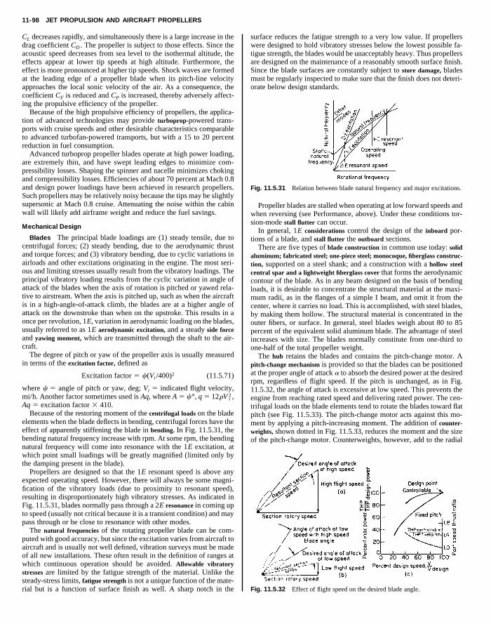
11-98 JET PROPULSION AND AIRCRAFT PROPELLERS
CL decreases rapidly, and simultaneously there is a large increase in thedrag coefficient CD . The propeller is subject to those effects. Since theacoustic speed decreases from sea level to the isothermal altitude, theeffects appear at lower tip speeds at high altitude. Furthermore, theeffect is more pronounced at higher tip speeds. Shock waves are formedat the leading edge of a propeller blade when its pitch-line velocityapproaches the local sonic velocity of the air. As a consequence, thecoefficient CF is reduced and CP is increased, thereby adversely affect-ing the propulsive efficiency of the propeller.
Because of the high propulsive efficiency of propellers, the applica-
surface reduces the fatigue strength to a very low value. If propellerswere designed to hold vibratory stresses below the lowest possible fa-tigue strength, the blades would be unacceptably heavy. Thus propellersare designed on the maintenance of a reasonably smooth surface finish.Since the blade surfaces are constantly subject to store damage, bladesmust be regularly inspected to make sure that the finish does not deteri-orate below design standards.
Copyright (C) 1999 by The McGraw-Hill Companies, Inc. All rights reserved. Use ofthis product is subject to the terms of its License Agreement. Click here to view.
tion of advanced technologies may provide turboprop-powered trans-ports with cruise speeds and other desirable characteristics comparableto advanced turbofan-powered transports, but with a 15 to 20 percentreduction in fuel consumption.
Advanced turboprop propeller blades operate at high power loading,are extremely thin, and have swept leading edges to minimize com-pressibility losses. Shaping the spinner and nacelle minimizes chokingand compressibility losses. Efficiencies of about 70 percent at Mach 0.8and design power loadings have been achieved in research propellers.Such propellers may be relatively noisy because the tips may be slightlysupersonic at Mach 0.8 cruise. Attenuating the noise within the cabinwall will likely add airframe weight and reduce the fuel savings.
Mechanical Design
Blades The principal blade loadings are (1) steady tensile, due tocentrifugal forces; (2) steady bending, due to the aerodynamic thrustand torque forces; and (3) vibratory bending, due to cyclic variations inairloads and other excitations originating in the engine. The most seri-ous and limiting stresses usually result from the vibratory loadings. Theprincipal vibratory loading results from the cyclic variation in angle ofattack of the blades when the axis of rotation is pitched or yawed rela-tive to airstream. When the axis is pitched up, such as when the aircraftis in a high-angle-of-attack climb, the blades are at a higher angle ofattack on the downstroke than when on the upstroke. This results in aonce per revolution, 1E, variation in aerodynamic loading on the blades,usually referred to as 1E aerodynamic excitation, and a steady side forceand yawing moment, which are transmitted through the shaft to the air-craft.
The degree of pitch or yaw of the propeller axis is usually measuredin terms of the excitation factor, defined as
Excitation factor 5 c(Vi /400)2 (11.5.71)
where c 5 angle of pitch or yaw, deg; Vi 5 indicated flight velocity,mi/h. Another factor sometimes used is Aq, where A 5 c°, q 5 12rV i
2 ,Aq 5 excitation factor 3 410.
Because of the restoring moment of the centrifugal loads on the bladeelements when the blade deflects in bending, centrifugal forces have theeffect of apparently stiffening the blade in bending. In Fig. 11.5.31, thebending natural frequency increase with rpm. At some rpm, the bendingnatural frequency will come into resonance with the 1E excitation, atwhich point small loadings will be greatly magnified (limited only bythe damping present in the blade).
Propellers are designed so that the 1E resonant speed is above anyexpected operating speed. However, there will always be some magni-fication of the vibratory loads (due to proximity to resonant speed),resulting in disproportionately high vibratory stresses. As indicated inFig. 11.5.31, blades normally pass through a 2E resonance in coming upto speed (usually not critical because it is a transient condition) and maypass through or be close to resonance with other modes.
The natural frequencies of the rotating propeller blade can be com-puted with good accuracy, but since the excitation varies from aircraft toaircraft and is usually not well defined, vibration surveys must be madeof all new installations. These often result in the definition of ranges atwhich continuous operation should be avoided. Allowable vibratorystresses are limited by the fatigue strength of the material. Unlike thesteady-stress limits, fatigue strength is not a unique function of the mate-rial but is a function of surface finish as well. A sharp notch in the
Fig. 11.5.31 Relation between blade natural frequency and major excitations.
Propeller blades are stalled when operating at low forward speeds andwhen reversing (see Performance, above). Under these conditions tor-sion-mode stall flutter can occur.
In general, 1E considerations control the design of the inboard por-tions of a blade, and stall flutter the outboard sections.
There are five types of blade construction in common use today: solidaluminum; fabricated steel; one-piece steel; monocoque, fiberglass construc-tion, supported on a steel shank; and a construction with a hollow steelcentral spar and a lightweight fiberglass cover that forms the aerodynamiccontour of the blade. As in any beam designed on the basis of bendingloads, it is desirable to concentrate the structural material at the maxi-mum radii, as in the flanges of a simple I beam, and omit it from thecenter, where it carries no load. This is accomplished, with steel blades,by making them hollow. The structural material is concentrated in theouter fibers, or surface. In general, steel blades weigh about 80 to 85percent of the equivalent solid aluminum blade. The advantage of steelincreases with size. The blades normally constitute from one-third toone-half of the total propeller weight.
The hub retains the blades and contains the pitch-change motor. Apitch-change mechanism is provided so that the blades can be positionedat the proper angle of attack a to absorb the desired power at the desiredrpm, regardless of flight speed. If the pitch is unchanged, as in Fig.11.5.32, the angle of attack is excessive at low speed. This prevents theengine from reaching rated speed and delivering rated power. The cen-trifugal loads on the blade elements tend to rotate the blades toward flatpitch (see Fig. 11.5.33). The pitch-change motor acts against this mo-ment by applying a pitch-increasing moment. The addition of counter-weights, shown dotted in Fig. 11.5.33, reduces the moment and the sizeof the pitch-change motor. Counterweights, however, add to the radial
Fig. 11.5.32 Effect of flight speed on the desired blade angle.

AIRCRAFT PROPELLERS 11-99
centrifugal load of the blades, necessitating a heavier retention, andconsequently do not necessarily reduce the net weight of the propeller.
Most pitch-change mechanisms employ a hydraulic piston, mountedon the hub, with feed through the propeller shaft and with rotation of theblades by means of gears or links. Electric motors and direct mechanicaldrives have been used successfully. In the past, the weight of all sys-tems, when fully developed, has turned out to be about the same.
Action of the pitch-change motor is limited by low- and high-pitchstops. These prevent the blades from assuming negative angles withreverse thrust. On reciprocating engines, the low-pitch stop is set to
maintain speed in rapid throttle movements, synchronizing to coordi-nate two or more engines, and with overriding features to activate thereversing and feathering sequences. (See also Sec. 16.)
Propeller controls are fundamentally the same, with several addedsecondary features. First, because the engine is capable of a very rapidincrease or decrease in torque and because of the high gear ratio be-tween the propeller and engine shaft, anticipating features are necessaryto prevent overspeeds in the propeller from producing large overspeedsand possible failure in the turbine. Second, because of the high idle rpmneeded to maintain the pressure ratio in the compressor, the low-pitch
Copyright (C) 1999 by The McGraw-Hill Companies, Inc. All rights reserved. Use ofthis product is subject to the terms of its License Agreement. Click here to view.
allow the propeller to absorb approximately rated power at zero forwardspeed. A lower setting results in higher windmilling drags in glidingflight, which could be dangerous if carried too far. In reversing pro-pellers the low-pitch stop is automatically removed when the controlsare set for reverse pitch. The high-pitch stop prevents the propeller fromreversing through the positive range. In feathering propellers it is set atthe angle which gives zero aerodynamic moment about the shaft.
Propeller feathering is provided in order to reduce the drag of a deadengine. To accomplish it, the blade-angle range is extended to 90°,approximately. Auxiliary pitch-change power is provided to completethe feathering as the engine slows down and to unfeather when theengine is stationary.
Fig. 11.5.33 Twisting effect of centrifugal loads on blades.
Reversing is provided in order to give propeller braking on the landingroll. It is accomplished by removing the flight low-pitch stop and driv-ing the blades to a high negative reverse-pitch angle. The principal me-chanical problem is to provide a mechanism which has the least possiblechance of going into reverse inadvertently.
The propeller control is that portion of the system which regulates theblade angle. In light aircraft, this may consist merely of a mechanismwhich sets a given blade angle corresponding to a given position of thecockpit control. In such cases the propeller acts as a fixed-pitch pro-peller except when activated by the pilot. In most cases, the propellercontrol regulates blade angle so as to maintain a preset rotary rpm,irrespective of flight speed or shaft power. The basic elements of thissystem normally consist of a spring-balanced, engine-drive flyweightdelivering an error signal which directs the servo, or pitch-changemotor, to increase or decrease blade angle (Fig. 11.5.34). The controlloop is closed by rpm feedback through the main engine. This basicsystem may be embellished with anticipating and delay devices to
stop of the turboprop engine propeller must be set substantially lowerthan for a piston engine. This is not true of a free-turbine drive and isonly partially true of a split-compressor engine. In the event of an enginefailure, the propeller, sensing the loss in rpm, will govern down to thelow-pitch stop. This may lead to large, often uncontrollable, negativethrust. To avoid this possibility, an engine-shaft torque signal is put intothe control, a negative torque automatically activating the featheringsystem. This portion of the system is known as the ENT (emergencynegative-thrust) system. Third, because of the high idle rpm characteris-tic of the turboprop engine, and the resulting low blade angles at lowpower in the ground-taxi regime, provision must be made to cut out thegoverning system and substitute direct blade-angle regulation (knownas beta control). This is required because the propeller will not governunder these conditions as the torque-to-blade-angle relationship goes tozero. The propeller control of a turboprop engine is normally mechani-cally coordinated directly to the engine throttle, leaving only a singlecontrol, with so-called power lever, in the aircraft.
Fig. 11.5.34 Propeller-speed governor.
The shaft on which the propeller is mounted is subjected to thesteady-thrust load, vibratory loads due to the propeller side, and gyro-scopic forces (the 1E moment, acting on the blades, is reactionless inpropellers with three or more blades). In large aircraft, the shaft size isusually determined by the propeller side force. In aircraft used for aero-batics, gyroscopic loads may become limiting. The gyroscopic momenton the propeller shaft is given by 2v1 ? v2(I1 2 I2), where v1 5 angularvelocity of maneuver, v2 5 angular velocity of shaft, I1 5 polar mo-ment of inertia of propeller about shaft, I2 5 moment of inertia ofpropeller about diameter in plane of rotation. (See also Sec. 3.)

11.6 ASTRONAUTICSby Aaron Cohen
REFERENCES: ‘‘Progress in Astronautics and Aeronautics,’’ AIAA series, Aca-demic Press. ‘‘Advances in Astronautical Sciences,’’ American Astronautical So-ciety series. ‘‘Handbook of the British Astronautical Association.’’ Koelle,‘‘Handbook of Astronautical Engineering,’’ McGraw-Hill. Purser, Faget, andSmith, ‘‘Manned Spacecraft: Engineering Design and Operation,’’ Fairchild Pub-lications. Herrick, ‘‘Astrodynamics,’’ Vol. 1, Van Nostrand Reinhold. Cohen,‘‘Space Shuttle,’’ Yearbook of Science and Technology, 1979, McGraw-Hill.
SPACE FLIGHTby Aaron Cohen
carrying of instruments for the measurement of the characteristics of(1) the environment through which the craft flies, (2) the surface ofthe celestial body over which the craft flies, or (3) astronomical objectsor phenomena. The commercial applications of space are now beingrealized. Many communication, weather, and earth-sensing satelliteshave been deployed. The space shuttle which provides a method to go
h orbits offers an expanded use of space.erials in a microgravity environment is proving to
icrogravity the effects of thermal convection and
External tank
Solid rocket booster (SRB)
Separation motors (each SRB), four a
Orbiter
Payload bay
Main engine (three)
Orbital maneuvering system engines
Reaction control system engines38 engines6 vernier rockets
* Includes spray-on foam insulation.
11-100
Copyright (C) 1999 by The McGraw-Hill Companies, Inc. All rights reserved. Use ofthis product is subject to the terms of its License Agreement. Click here to view.
to and from low eartProcessing of mat
be very reliable. In m
gravity are eliminated, hence purer materials can be manufactured.S
The science of astronautics deals with the design, construction, andoperation of craft capable of flight through interplanetary or interstellarspace. In addition to orbits around, and trajectories between, suchbodies as stars, planets, and planetoids, the ascents from and descents tothe surface of such bodies are considered to be part of the field.
The purposes of such craft are numerous and include the transporta-tion of people and cargo, the transmission or relaying of signals, and the
Table 11.6.1 Specifications of the Space Shuttle
Component
Overall system
ft, four forward
(two)
Containerless processing can also be accomplished which will lead toadditional applications in microgravity materials technology. The spaceshuttle allows payloads up to 32,000 lb to be placed in earth orbit ataltitudes of 150 to 200 nautical miles (nmi) and inclinations of 28.5° to90°. A description of the space shuttle is contained in Table 11.6.1.Using expendable launch vehicles or the space shuttle and propulsion-assistance modules, satellites can be placed in various orbits. A polarorbit is one whose orbital plane includes the earth’s axis and permits
ystem and Its Components
Characteristic Specifications
Length 184.2 ft (56.1 m)Height 76.6 ft (23.3 m)System weightDue-east launch 4,490,800 lbm (2037.0 Mg)104° launch azimuth 4,449,000 lbm (2018.0 Mg)
Payload weightDue-east launch 65,000 lbm (29.5 Mg)
104° launch azimuth 32,000 lbm (14.5 Mg)Diameter 27.8 ft (8.5 m)*Length 154.4 ft (47.1 m)WeightLaunch 1,648,000 lbm (747.6 Mg)Inert 70,990 lbm (32.2 Mg)
Diameter 12.2 ft (3.7 m)Length 149.1 ft (45.4 m)Weight (each)Launch 1,285,100 lbm (582.9 Mg)Inert 176,300 lbm (80.0 Mg)
Launch thrust (each) 2,700,000 lbf (12.0 MN)
Thrust (each) 22,000 lbf (97.9 kN)
Length 121.5 ft (37.0 m)Wingspan 78.1 ft (23.8 m)Taxi height 57 ft (17.4 m)WeightInert 161,300 lbm (73.2 Mg)LandingWith payload 203,000 lbm (92.1 Mg)Without payload 173,000 lbm (78.5 Mg)
Cross range 1,100 nmi (2037.2 km)
Length 60 ft (18.3 m)Diameter 15 ft (4.6 m)
Vacuum thrust (each) 470,000 lbf (2090.7 kN)
Vacuum thrust (each) 6,000 lbf (26.7 kN)
Vacuum thrust (each) 870 lbf (3870 N)Vacuum thrust (each) 24 lbf (111.2 N)

ASTRONOMICAL CONSTANTS OF THE SOLAR SYSTEM 11-101
line-of-sight contact between the spacecraft and every point on earth ona periodic basis. Synchronous orbits have angular rates equal to therotational rate of the earth about its axis, providing a spacecraft locus ofpositions at nearly constant longitude. Orbital-parameter variation pro-vides a wide variety of other orbits, permitting the selection of charac-teristics most suitable for the specific flight objective, such as commu-nication relays, meteorological observations, earth surface monitoring,or interplanetary trajectories.
Rep. 32-604, Jet Propulsion Lab., Pasadena. Francis, Constants for an Earth-Moon Transit, Lockheed Rep. LAC/421571. Krause, On a Consistent System ofAstrodynamic Constants, NASA-TN D-1642. Makemson, Baker, and Westrom,Analysis and Standardization of Astrodynamic Constants, Jour. Astro. Sci.,Spring 1961. Townsend, ‘‘Orbital Flight Handbook,’’ Martin Co. Space and Plan-etary Environment Criteria Guidelines for Use in Space Vehicle Develop-ment, 1982 Revision (Vols. I and II), NASA Technical Memoranda 82478 and82501.
A greater number of astronomical constants is used in astrodynamicsand astronautics than in classic astronomy because astronautics is a kind
55
qui
50T
Copyright (C) 1999 by The McGraw-Hill Companies, Inc. All rights reserved. Use ofthis product is subject to the terms of its License Agreement. Click here to view.
ASTRONOMICAL CONSTANTSOF THE SOLAR SYSTEMby Michael B. DukeNASA
REFERENCES: ‘‘Handbook of the British Astronautical Association.’’ Blancoand McCuskey, ‘‘Basic Physics of the Solar System,’’ Addison-Wesley.Clarke, Constants and Related Data for Use in Trajectory Calculations, Tech
Table 11.6.2 General, Terrestrial, and Lunar Constants
1. Ephemeris second: 1 secE 5 1/31,556,925.9747 of tropical year at 1900.0.2. Mean solar day (culmination period of the mean sun):
1d 5 1d*(.002 737 909 265 1 0d*.589 3 10210T5 1rot.002 737 811 891 2 0rot.001 4 3 10210T
3. Mean sidereal day or mean equinoctial day (culmination period of the vernal e
1d* 5 0d.997 269 566 414 2 0d.587 3 10210T5 0rot.999 999 902 892 2 0rot.589 3 1021
4. Mean stellar day or mean period of the earth’s rotation (culmination period of an
1dst 5 1rot 5 1d*.000 000 097 108 1 0d*.589 3 10
5 24h*00m*.008 390 13 1 0 s*.050 89 35 0d.997 269 663 257 1 0d.001 4 3 102
5. Tropical year (equinox to equinox):
Ptrop 5 (365.242 198 78 2 0.000 006
6. Sidereal year (fixed star to fixed star):
Psid 5 (365.256 360 42 1 0.000 000 11
7. Synodic month (new moon to new moon):
Psyn 5 (29.530 588 2 2 0.000 000 2 T
8. Tropical month (equinox to equinox):
Ptrop 5 (27.321 581 7 2 0.000 000 2
9. Sidereal month (fixed star to fixed star):
Psid 5 (27.321 661 0 2 0.000 000 2 T
10. Astronomical unit (mean earth-sun distance): au 5 149,598,700 6 400 km.11. Light year: ly 5 (9.460 530 6 0.000 003) 3 1012 km 5 63,239.39 6 0.15 au.12. Parsec: pc 5 206,264.806 247 au 5 (3.085 695 6 0.000 008) 3 1013 km.13. Semimajor axis of the earth’s orbit: a! 5 1.000 000 236 au 5 149,598,700 6 414. Mean orbital speed: v! 5 29,784.90 6 0.08 m/sec.15. Mass of the earth: M! 5 (5.9761 6 0.004 3) 3 1024 kg.16. Equatorial radius of the earth: Re! 5 6,378 170 6 20 m.17. Flattening (oblateness, ellipticity): f! 5 (Re 2 Rp)/Re 5 0.003 352 55 5 1:(29818. Acceleration of gravity at the earth’s surface:
g 5 ge(1 1 b sin2 f 1 g sin2 2f) 5 9.780 315(1 1
19. Moments of inertia of the earth:
A 5 (0.329 6814 6 0.000 11) M ! Re2
C 5 (0.330 7639 6 0.000 11) M ! Re2
20. Circular and escape velocities from the earth’s surface at the equator.
vcir 5 7,905.39 6 0.06 m/sec vesc
21. Mean observed distance of the perturbed moon from the earth:
r 5 384,401.0 6 1.0 km 5 (60.268 23 6 0.00
22. Semimajor axis of the moon’s orbit: a 5 1.000 907 681r 5 384 749.9 6 1.023. Mean orbital velocity: v 5 1,024.089 6 0.003 m/sec.24. Mass of the moon: M 5 (7.353 4 6 0.007 5) 3 1022 kg 5 M !: (81.270 6 0.25. Semiaxes of the moon ellipsoid: a 5 1,738,780 6 186 m; b 5 1,738,452 6 209 m
The time T is in Julian centuries of 36,525 days from 1900 Jan. 0.5 U.T. (univers
of experimental astronomy and its missions vary so greatly. A higheraccuracy is also necessary because the astrodynamic missions includedeparture, landing, and flyby maneuvers. Some of the constants, givenin relative and astronomical units in celestial mechanics, must be knownin absolute units for astrodynamic purposes. Tables 11.6.2 to 11.6.4provide the latest observed data for standardization of astrodynamiccomputations. See references for additional constants.
24h*03m*56 s*.555 360 50 1 0 s*.050 89 3 1024T(1 6 1028)d
E
nox):
23h56m04 s.090 538 17 2 0 s.050 716 8 3 1024T
equatorial star without proper motion):
210T1024T
10T 5 23h56m04 s.098 905 40 1 0 s.001 21 3 1025T
138 T )dE 5 365d
E 05hE 48E
m45 sE .530 T
T )dE 5 365d
E 06hE 09E
m09 sE .54 1 0 s
E .010 T
)d 5 29d 12h 44m02 s .78 2 0 s.017 T
T )d 2 27d 07h 43m04 s .7 2 0 s.017 T
)d 5 27d 07h 43m11 s .47 2 0 s.017 T
00 km.
.28 6 0.05).
0.005 302 74 sin2 f 2 0.000 005 9 sin2 2f) m/sec2
5 (0.801 50 6 0.000 85) 3 1038 kg-m2
5 (0.804 13 6 0.000 85) 3 1038 kg-m2
5 vcir21/2 5 11,179.91 6 0.08 m/sec
0 35) Re! 5 0.002 569 548 6 0.000 000 014 au
km.
024).; c 5 1,737,688 6 188 m.
al time). The constants are given with probable errors (pe).

11-102A
ST
RO
NA
UT
ICS
Table 11.6.3 Planetary Orbit Data
Mean PlanetaryNumber Semimajor Sidereal Synodic Mean daily Inclination ascending Longitude Orbital escape Gravity at
of axis, period, period, motion, Eccentricity, to ecliptic, node V, perihelion, speed, speed, surface,Planet satellites au year days s/day e i, deg deg v, deg km/s km/s cm/s2
0.387 0.2411 115.88 14,732.42 0.206 7.004 47.857 76.833 47.8 4.3 3700.723 0.6152 583.92 5767.2 0.007 3.394 76.320 131.008 35.0 10.3 887
1 1.0000 1.0000 3548.19 0.017 102.253 29.8 11.2 9822 1.524 1.8822 779.94 1886.52 0.093 1.850 49.250 335.322 24.2 5.0 372
16 5.203 11.86 398.88 299.13 0.048 1.305 99.44 12.72 13.1 61 259915 9.54 29.46 378.09 120.46 0.056 2.490 113.307 92.264 9.7 39.4 12905 19.2 84.0 369.66 42.23 0.50 0.773 73.796 170.011 6.8 21.2 8302 30.1 164.8 367.49 21.53 0.009 1.774 131.340 44.274 5.4 23.8 13801 39.7 247.7 366.74 14.29 0.249 17.170 109.886 112.986 4.7 ; 1.3
MercuryVenusEarthMarsJupiterSaturnUranusNeptunePluto
Copyright (C
) 1999 by The M
cGraw
-Hill C
ompanies, Inc. A
ll rights reserved. Use of
this product is subject to the terms of its L
icense Agreem
ent. Click here to view
.

DYNAMIC ENVIRONMENTS 11-103
Table 11.6.4 Physical Data of Sun, Moon, and Planets
Polar Mean InclinationEquatorial radius, density, Visual Rotational of equator
Name radius, km km Mass, kg g/cm3 albedo period to orbit, deg
Sun 696,000 1.99 3 1030 1.42 ; 27 days 7.25Moon 1,738 7.35 3 1022 3.34 0.067 27.322 days 6.65Mercury 2,439 3.30 3 1023 5.44 0.235 58.646 days , 1Venus 6,051 4.87 3 1024 5.24 0.80 243.0 days 2.2Earth 6,378 6,356 5.98 3 1024 5.52 0.39 23.93 h 23.45Mars 3,397 3,375 6.42 3 1023 3.93 0.1–0.4 24.62 h 25Jupiter 71,398 66,793 1.89 3 1027 1.32 0.51 9.92 h 3.1Saturn 60,330 55,020 5.68 3 1026 0.71 0.45 10.66 h 26.7Uranus 26,145 25,518 8.73 3 1025 1.2 0.56 11–24 h 97.9Neptune 24,700 24,060 1.03 3 1026 1.67 0.57 ; 18 h 28.8Pluto 1,600 1.4–2 3 1022 0.55–1.75 0.25–0.5 ? ?
DYNAMIC ENVIRONMENTSby Michael B. DukeNASA
REFERENCES: Harris and Crede, ‘‘Shock and Vibration Handbook,’’ McGraw-Hill. Beranek, ‘‘Noise Reduction,’’ McGraw-Hill. Crandall, ‘‘Random Vibra-tion,’’ Technology Press, MIT. Neugebauer, The Space Environment, Tech. Rep.34-229, Jet Propulsion Lab., Pasadena, 1960. Hart, Effects of Outer Space Envi-ronment Important to Simulation of Space Vehicles, AST Tech Rep. 61-201. Cor-nell Aeronautical Lab. Barret, Techniques for Predicting Localized Vibratory En-
The sound-generation mechanism is presented in empirical and ana-lytical form, utilizing measured sound pressures and the known engineoperational parameters. This combination of empirical terms and ana-lytical reasoning provides a generalized relationship to predict sound-pressure levels for the vehicle structure and also for far-field areas. Ithas been shown by Lighthill (Proc. Royal Soc., 1961) that acoustic-power generation of a subsonic jet is proportional to rV 8D2/a3
0 , where ris the density of the ambient medium, a0 is the speed of sound in theambient medium, V is the jet or rocket exit exhaust velocity, and D is acharacteristic dimension of the engine. Attempts have been made to
Copyright (C) 1999 by The McGraw-Hill Companies, Inc. All rights reserved. Use ofthis product is subject to the terms of its License Agreement. Click here to view.
vironments of Rocket Vehicles, NASA TN D-1836. Wilhold, Guest, and Jones, ATechnique for Predicting Far Field Acoustic Environments Due to a MovingRocket Sound Source, NASA TN D-1832. Eldred, Roberts, and White, StructuralVibration in Space Vehicles, WADD Tech. Rep. 61–62. Bolt, Beranek, and New-man, Exterior Sound and Vibration Fields of a Saturn Vehicle during Static Firingand during Launching, U.S.A. Ord. Rep. 764.
The forces required to propel a space vehicle from the launch pad aretremendous. The dynamic pressures generated in the atmosphere bylarge rocket engines are exceeded only by nuclear blasts. Slow initialascent from the launch pad is followed by rapid acceleration and high gloading, and acoustic and aerodynamic forces drive every point of thevehicle surface. The space-vehicle velocity quickly becomes supersonicand continues to hypersonic velocities. Gradually, as the space vehicleleaves the atmosphere, the aerodynamic forces recede. Then suddenlythe rocket thrust decays and is followed by the ignition of anotherrocket, which quickly develops thrust and continues to accelerate thespace vehicle. Finally, the space vehicle becomes weightless. In com-pleting a mission, a space vehicle is subjected to the additional environ-mental extremes of planetary landings, escape, and earth reentry.
These environments represent basic criteria for space-vehicle design.For operational reliability, the most important are the shock, vibration,and acoustic environments which are present to varying magnitudes inall operational phases and which constitute major engineering prob-lems.
It is not possible to have original environmental data prior to fabrica-tion and testing of a particular structure. Vibration, shock, and acousticnoise adversely affect structural integrity and vehicle reliability. Theseenvironments must be considered prior to design and fabrication andthen again for design verification through ground testing. Precise vibra-tion and acoustic environmental predictions are complicated because ofstructural nonlinearities, random forcing functions, and multiple-degree-of-freedom systems. Current environmental-prediction tech-niques consist mainly of extrapolating measured data obtained fromexisting vehicles. Acoustic environments produced during ground testare important factors in evaluating ground-facility locations and de-sign, personnel safety, and public relations.
A source of sound common to all jet and rocket-engine propulsionsystems is the turbulent exhaust flow. This high-velocity flow producespressure fluctuations, referred to as noise, and has adverse effects on thevehicle and its operations. Also, far-field uncontrolled areas may besubjected to intense acoustic-sound-pressure levels which may requirepersonnel protection or sound-suppression devices. (See also Sec. 12.)
extend this relationship to allow supersonic-jet acoustic-power predic-tions to be made, but no one scheme is accepted for broad use.
From acoustic-data-gathering programs utilizing rocket engines,various trends have been noted which facilitate acoustic predictions. Forrocket engines of up to 5 3 109 W mechanical power, the acousticefficiency shows a nonlinear rate of increase. For greater mechanicalpower, the acoustic efficiency approaches a value slightly higher than0.5 percent (Fig. 11.6.1).
Fig. 11.6.1 Acoustic-efficiency trends.
Turbulent-exhaust-flow sound-source mechanisms also exhibit di-rectional characteristics. Figure 11.6.2 shows data from a Saturn rocketvehicle launch with the microphone flush-mounted on the vehicle skinat approximately 100 ft above the nozzle plane.
During the period between on-pad firing and post-lifting-off or main-stage flight, the exhaust-flow direction changes. The directivity has alsoshifted 90° to retain its inherent relationship to the exhaust stream. Thesound-pressure-level variation during a small time interval—between
Fig. 11.6.2 Vehicle acoustic environment.

11-104 ASTRONAUTICS
The sources of vibration excitation are (1) acoustic pressures gener-ated by rocket-engine operation; (2) aerodynamic pressures created byboundary-layer fluctuations; (3) mechanically induced vibration fromrocket-engine pulsation, which is transmitted throughout the vehiclestructure; (4) vibration transmitted from adjacent structure; and (5) lo-calized machinery. Since the mean square acceleration is proportionalto power, the total vibrational power at any point on the vehicle may beexpressed as
Pv 5 Pv(1) 1 Pv(2) 1 Pv(3) 1 Pv(4) 1 Pv(5)
Copyright (C) 1999 by The McGraw-Hill Companies, Inc. All rights reserved. Use ofthis product is subject to the terms of its License Agreement. Click here to view.
Fig. 11.6.3 Random-vibration spectrum of a space-vehicle structure.
on-pad condition and shortly after liftoff—depends on the changeswhich have occurred in the directivity and the jet-exhaust-velocity vec-tor (Fig. 11.6.2). The change in sound-pressure level is 20 dB approxi-mately in this case and is indicative of the significance of a soundsource’s directional properties, which depend on velocity and temper-ature of the jet.
The acoustic environments produced by a given conventional enginecan be empirically described by that engine’s flow parameters and ge-ometry. It is difficult to predict the acoustic environments for noncon-ventional engines such as the plug-nozzle and expansion-deflection en-gines.
The turbulent-boundary-layer problem of high-velocity vehicleflights is difficult to evaluate in all but the simplest cases. Only forattached, homogeneous, subsonic flows can the boundary-layer noise beestimated with confidence.
The vibratory environment on rocket vehicles consists of total-vehicle bending vibrations, in which the vehicle is considered a non-uniform beam, with low-frequency responses (0 to 20 Hz) and localizedvibrations with frequencies up to thousands of hertz. (See alsoSec. 5.)
The response of a simple structure to a dynamic forcing function maybe described by the universal equation of motion given as ~M ~x 1 c ~x 1Kx 5 F(t) or F(t)x(t) 5 (M 2 Kv2) 2 j(c/v) and is a complex functioncontaining real and imaginary quantities. In the case of rocket-vehiclevibrations, F(t) is a random forcing phenomenon. Thus, the motionresponses must also be random. Random vibration may be described asvibration whose instantaneous magnitudes can be specified only byprobability-distribution functions giving the probable fraction of thetotal time that the magnitude, or some sequence of magnitudes, lieswithin a specified range. In this type of vibration, many frequencies arepresent simultaneously in the waveform (Fig. 11.6.3). Power spectraldensity (PSD; in units of g2/Hz) is defined as the limiting mean-squarevalue of a random variable, in this case acceleration per unit bandwidth;i.e.,
PSD 5 limDf:0
g 2/Df 5 dg 2/df
Fig. 11.6.4 Sources of vibration excitement.
This is illustrated in Fig. 11.6.4 for an arbitrary vehicle. In manyinstances, the structure is principally excited by only one of thesesources and the remaining can be considered negligible (Fig. 11.6.5).The vibration characteristics of structure B, taken from a skin panel,closely correspond to the trends of the acoustic pressures during flight.However, structure A, taken from a rocket-engine component, exhibitsstationary trends, indicating no susceptibility to the impinging acousticfield. Thus, for this structure, it can be assumed that only Pv(3) issignificant, whereas for structure B, only Pv(1) is the principal excitingsource during the on-pad phase and only Pv(2) is significant during themaximum dynamic-pressure phase. This also holds true for captive fir-ings of the vehicle, in which only Pv(1) is significant for structure B andPv(3) for structure A.
Fig. 11.6.5 Typical structural responses to a random-vibration environment.
SPACE-VEHICLE TRAJECTORIES, FLIGHTMECHANICS, AND PERFORMANCEby O. Elnan, W. R. Perry, J. W. Russell,A. G. Kromis, and D. W. FellenzUniversity of Cincinnati
REFERENCES: Russell, Dugan, and Stewart, ‘‘Astronomy,’’ Ginn. Sutton,‘‘Rocket Propulsion Elements,’’ Wiley. White, ‘‘Flight Performance Handbookfor Powered Flight Operations,’’ Wiley. ‘‘U.S. Standard Atmosphere, 1962,’’NASA, USAF, U.S. Weather Bureau. Space Flight Handbooks, NASA SP-33,SP-34, and SP-35. Gazley, Deceleration and Heating of a Body Entering a Plane-tary Atmosphere from Space, ‘‘Visits in Astronautics,’’ Vol. I, Pergamon. Chap-man, An Approximate Analytical Method for Studying Entry into Planetary At-mospheres, NACA-TN 4276, May 1958. Chapman, An Analysis of the Corridorand Guidance Requirements for Super-circular Entry into Planetary Atmospheres,NASA-TN D-136, Sept 1959. Loh, ‘‘Dynamics and Thermodynamics of PlanetaryEntry,’’ Prentice-Hall. Grant, Importance of the Variation of Drag with Lift inMinimization of Satellite Entry Acceleration, NASA-TN D-120, Oct. 1959. Lees,Hartwig, and Cohen, Use of Aerodynamic Lift during Entry into the Earth’s At-mosphere, Jour. ARS, 29, Sept 1959. Gervais and Johnson, Abort during MannedAscent into Space, AAS, Jan. 1962.
Notation
A 5 reference areaAz 5 launch azimuthB 5 ballistic coefficient
CL 5 lift coefficient

ORBITAL MECHANICS 11-105
e 5 eccentricityf 5 stage-mass fraction (WP/WA)
H 5 total energyH` 5 hyperbolic excess energy
I 5 specific impulseDi 5 plane-change angleL 5 lift forcem 5 massn 5 mean motion (2p/psid)p 5 ambient atmospheric pressure
o 5 sea level conditions at 45° latitudes 5 space fixed
vac 5 vacuumcirc 5 circular orbital conditionesc 5 escape
i 5 initialp 5 perigee
M 5 meanSL 5 sea levelsid 5 sidereal
Copyright (C) 1999 by The McGraw-Hill Companies, Inc. All rights reserved. Use ofthis product is subject to the terms of its License Agreement. Click here to view.
q 5 dynamic pressureR 5 earth’s equatorial radiusS 5 wing areaT 5 transfer time, time, absolute temperature
tpp 5 time after perigee passageVc 5 injection velocityV 5 velocity
Vg 5 velocity loss to gravityW 5 weight
WL 5 payload weightWP 5 propellant weight
Y 5 distanceaV 5 right ascension of the ascending node
g 5 u 2 90° 5 flight-path angle used in reentry analysisv 5 true anomalyv 5 earth’s rotational velocityc 5 central angle
s 5 r/r0 5 relative atmospheric densityY 5 vernal equinoxAe 5 nozzle exit areaa 5 semimajor axis
CD 5 drag coefficientD 5 drag forceE 5 eccentric anomalyF 5 thrustg 5 acceleration due to gravity
Hesc 5 escape energyh 5 altitudei 5 inclination
J2 5 oblateness coefficient of the earth’s potential(second-zonal harmonic)
M 5 molecular weight, mean anomalynm 5 nautical miles
P 5 period of revolutionPe 5 nozzle exit pressureqs 5 stagnation-point heat-transfer rater 5 radiuss 5 ranget 5 time
V` 5 hyperbolic excess velocityVid 5 ideal velocityDV 5 impulsive velocityWA 5 stage weight (WO 2 WL)WO 5 gross weight
X 5 distancea 5 angle of attack, right ascensionb 5 exponent of density-altitude functionl 5 longitudet 5 hour anglev 5 argument of perigee
f9 5 latituder 5 atmospheric densityu 5 flight-path angle
Subscripts
a 5 apogeee 5 entryf 5 final
ORBITAL MECHANICSby O. Elnan and W. R. PerryUniversity of Cincinnati
The motion of the planets about the sun, as well as that of a satellite inits orbit about a planet, is governed by the inverse-square force law forattracting bodies. In those cases where the mass of the orbiting body issmall relative to the central attracting body, it can be neglected. Thissimplifies the analysis of the orbital motion. The shape of the orbit isalways a conic section, i.e., ellipse, parabola, or hyperbola, with thecentral attracting body at one of the foci. Parabolic and hyperbolic orbitsare open, terminate at infinity, and represent cases where the orbitingbody escapes the central force field of the attracting body.
The laws of Kepler for satellite orbits are (1) the radius vector to thesatellite from the central body sweeps over equal areas in equal times;(2) the orbit is an ellipse, with the central attracting body at one of itsfoci; and (3) the square of the period of the satellite is proportional to thecube of the semimajor axis of the orbit.
Six orbital elements are required to describe the orbit in the orbit planeand the orientation of the plane in inertial space. The three elements thatdefine the orbit are the semimajor axis a, eccentricity e, and period ofrevolution P. The orientation of the orbit (Fig. 11.6.6) is defined by the
Fig. 11.6.6 Elements of satellite orbit around a planet.
right ascension of the ascending node aV , inclination of the orbit planeto the earth’s equatorial plane i, and the argument of perigee v, which isthe central angle measured in the orbit plane from ascending node toperigee. The following equations compute these orbital elements andother orbital parameters.
a 5 (ra 1 rp)/2 5 m /VaVp 5 ra/(1 1 e) 5 rp /(1 2 e)e 5 (ra /a) 2 1 5 (Vp 2 Va)/(Vp 1 Va) 5 (rpV 2
p /m) 2 1r 5 a(1 2 e2)/(1 1 e cos n)
ra 5 a(1 1 e) 5 rp(1 1 e)/(1 2 e)rp 5 a(1 2 e) 5 ra(1 2 e)/(1 1 e)V 5 [m(2/r 2 1/a)]0.5
P 5 2p(a3m)0.5 (for circular orbits, r 5 a)Va 5 Vp(1 2 e)/(1 1 e) 5 [m(1 2 e)/a(1 1 e)]0.5
Vp 5 Va(1 1 e)/(1 2 e) 5 [m(1 1 e)/a(1 2 e)]0.5
n 5 cos2 1{[2rarp 2 r(ra 1 rp)]/r(ra 2 rp)}tpp 5 (a3/m)0.5{cos2 1[(a 2 r)/ae]
2 e[1 2 (a 2 r)2/(ae)2]0.5}M 5 ntpp 5 E 2 e sin Er 5 a(1 2 e cos E)
Vesc 5 (2m/r)0.5

11-106 ASTRONAUTICS
The elements may be determined from known injection conditions.For example,
1/a 5 V 2im 2 2/ri
e2 5 cos2 Vi(riV 2i /m 2 1)2 1 sin2 Vi
General precession in longitude of vernal equinox:
x 5 5099.2575 1 099.0222T
where T is in Julian centuries of 36,525 mean solar days reckoned from
2/(ri 1 rf )]}0.5 2 (m/ri)0.5 and DVf 5 (m/rf )0.5 2 {m[2/rf 2 2/(ri 1rf )]}0.5, where Vi is the orbiting velocity in low orbit and Vf is theorbiting velocity in the high orbit.
Orbital Lifetime The satellite orbit will gradually decay to loweraltitudes because of the drag effects of the atmosphere. This drag forcehas the form D 5 1⁄2CDArV 2, where values of the drag coefficient CD
may range from 2.0 to 2.5. The atmospheric density, as a function ofaltitude, can be used for computing an estimated orbital lifetime of asatellite (Fig. 11.6.8). (See NASA, ‘‘U.S. Standard Atmosphere’’ and‘‘Space Flight Handbooks.’’)
Copyright (C) 1999 by The McGraw-Hill Companies, Inc. All rights reserved. Use ofthis product is subject to the terms of its License Agreement. Click here to view.
1900 Jan. 0.5 UT.
Measurement of Time
The concept of time is based on the position of celestial bodies withrespect to the observer’s meridian as measured along the geocentriccelestial equator. The mean sun and the vernal equinox (Y) are used todefine mean solar time and sidereal time. The mean sun, rather than theapparent (true) sun, is used since the latter’s irregular motion frommonth to month gives a variation in the length of a day. The mean sunmoves with uniform speed along the equator at a rate equal to theaverage of the true sun’s angular motion during the year.
One sidereal day is the interval between two successive transits of thevernal equinox across the observer’s meridian. A mean solar day is theinterval between two successive transits of the mean sun. Local civiltime (LCT) is defined to be the hour angle of the mean sun plus 12 h.Local sidereal time is the hour angle of the vernal equinox plus 12 h.For an observer at the Greenwich meridian, the local civil time isGreenwich mean time (GMT) or universal time (UT). The earth isdivided into 24 time zones, each 15° of longitude wide. Each zone keepsthe time of the standard meridian in the middle of the zone. (See Fig.11.6.7.)
Time T 5 t 1 12 hLocal sidereal time LST 5 tY 1 12 hGreenwich sidereal time GST 5 LST 1 l(w)Local civil time LCT 5 tM 1 12 h 5 mean solar timeEquation of time ET 5 t 2 tM 5 aM 2 aGreenwich mean time GMT 5 UT 5 tM(Greenwich) 1 12 h 5
universal time
LCT 5 UT 2 l(w)GMT 5 ZT 6 l°/15
The ‘‘American Ephemeris and Nautical Almanac’’ gives the equa-tion of time for every day of the year and conversions of mean solar timeto and from sidereal time.
Hohmann Transfer This is a maneuver between two coplanar orbitswhere the elliptical transfer orbit is tangent at its perigee to the lowerorbit and tangent at its apogee to the higher orbit. To transfer from a lowcircular orbit to a higher one, the impulsive velocity required is thedifference between the velocities in the circular orbits and the velocitiesin the corresponding points on the transfer orbit. Using the generalvelocity equation above, the transfer velocities are DVi 5 {m[2/ri 2
Fig. 11.6.7 Time-zone geometry.
Fig. 11.6.8 Satellite lifetimes in elliptic orbits. r 5 ARDC, 1959; B 5CDA/2m 5 1.0 ft2/slug; e 5 initial eccentricity; --- 5 decay histories.
Perturbations of Satellite Orbits There are many secular and peri-odic perturbations of satellite orbits due to the effects of the sun, themoon, and some planets. The most significant perturbation on close-earth satellite orbits is caused by the oblateness of the earth. Its great-est effects are the precession of the orbit along the equator (nodal re-gression) and the rotation of the orbit in the orbit plane (advanceof perigee). The nodal-regression rate is given to first-order approxima-tion by
~aV 5 2 3⁄2(m/a3)0.5J2[R/a(1 2 e2)]2 cos i
The mean motion of the perigee is
~v 5 J2n(2 2 (5⁄2) sin2i)/a2(1 2 e2)2
LUNAR- AND INTERPLANETARY-FLIGHTMECHANICSby J. W. RussellUniversity of Cincinnati
The extension of flight mechanics to the areas of lunar and interplane-tary flight must include the effects of the sun, moon, and planets on thetransfer trajectories. For most preliminary performance calculations, the‘‘sphere-of-influence,’’ or ‘‘patched-conic,’’ method—whereby the multi-body force field is treated as a series of central force fields—providessufficient accuracy. By this method, the trajectories in the central forcefield are calculated to the ‘‘sphere of influence’’ of each body as stan-dard Keplerian mechanics, and the velocity and position of the extre-mals are then matched to give a continuous trajectory. After the mis-sions have been finalized, the precision trajectories are obtained bynumerically integrating the equations of motion which include all theperturbative elements. It is necessary to know the exact positions of thesun, moon, and planets in their respective orbits.

ATMOSPHERIC ENTRY 11-107
Lunar-Flight Mechanics The moon moves about the earth in anorbit having an eccentricity of 0.055 and an inclination to the ecliptic ofabout 5.145°. The sun causes a precession of the lunar orbit about theecliptic, making the inclination of the lunar plane to the earth’s equato-rial plane oscillate between 18.5 and 28.5° over a period of 18.5 yearsapprox. To compute precision earth-moon trajectories, it is necessary toknow the precise launch time to be able to include the perturbativeeffects of the sun, moon, and planets. The data presented are based onthe moon being at its mean distance from earth and neglect the pertur-bation of the sun and planets; they are therefore only to be considered as
2
2
1
about the sun so as to arrive at the target planet at the desired positionand time. The energy required to escape the gravitational attraction of aplanet can be determined by Keplerian mechanics to be Hesc 5 m/r,where m is the gaussian gravitational constant and r is the distance fromthe center of the planet. After escaping the departure planet, the velocitymust be altered in both magnitude and direction—in order to arrive atthe target planet at the chosen time—by supplying additional energy,H` 5 1⁄2V 2
` .For determination of vehicle size necessary to inject the spacecraft
into the interplanetary trajectory, it is convenient to express the total
Copyright (C) 1999 by The McGraw-Hill Companies, Inc. All rights reserved. Use ofthis product is subject to the terms of its License Agreement. Click here to view.
representative data. The injection velocity (see Gazley) at 100 nmi forearth-moon trajectories and the impulsive velocity for braking into a100-nmi orbit about the moon are shown in Fig. 11.6.9 as a function oftransfer time. Additional energy is required to offset losses due to grav-ity and aerodynamic drag as well as to provide plane-change andlaunch-window capabilities.
Fig. 11.6.9 Lunar-mission velocity requirements.
Interplanetary-Flight Mechanics The fact that planetary orbitsabout the sun are not coplanar greatly restricts the number of feasibleinterplanetary trajectories. The plane of the interplanetary trajectorymust include the position of the departure planet at departure, the sun,and the position of the target planet at arrival. The necessary planechange can be prohibitive even though the relative inclinations of theplanetary orbits are small. The impulsive velocity required to effect aplane change for a spacecraft departing earth can be approximated byDV 5 195,350 sin (Di /2), where Di is the amount of plane changerequired and DV is in ft /s.
For interplanetary flight, the ‘‘ideal’’ total energy that must be im-parted to the spacecraft is the energy required to escape the gravitationalfield of the departure planet plus the energy required to change path
Table 11.6.5 Hyperbolic-Excess-Velocity Requirements(ft/s) for Typical Mars Missions
Opposition yearTrip time,
days 1982 1984 1986 1988 1990
100 27,241 23,012 18,070 15,569 19,955150 15,940 13,088 11,437 10,520 13,792200 12,268 10,021 11,486 9,308 12,463250 10,510 12,688 13,410 10,480 15,784
SOURCE: Gammal, ‘‘Space Flight Handbooks.’’
Table 11.6.6 Planetary Atmospheres
Vesc , M,Planet ft /s Gases gmol21
Venus 34,300 2% N2 4098% CO2
Earth 36,800 78% N2 2921% O2
Mars 16,900 95% N2 283% CO
2Jupiter 195,000 89% H2 2.2 111% He
rSL ,T, K b21, ft bt lb/ft3
50–350 2 3 104 1,006 1.0
40 2.35 3 104 880 0.0765
30–300 6 3 104 132 0.0062
energy H 5 Hesc 1 H` in terms of the required injection velocity
Vc 5 √2(Hesc 1 H`) or Vc √(2m/r) 1 V 2`
Hyperbolic excess velocities V` for earth-to-Mars missions are shownin Table 11.6.5 as a function of date. These velocities are near optimumfor the trip time and year given but do not represent absolute-optimumtrajectories. Mars has a cyclic period with respect to earth of 17 yearsapprox; hence the energy requirements for Mars missions from earthalso follow approximate 17-year cycles.
Figure 11.6.10 shows how the hyperbolic excess velocities of Table11.6.5 can be converted to stage characteristic velocities for a vehicleleaving a 100-nmi earth parking orbit. These are simple cases. In manyrecent planetary missions, use has been made of planetary flybys to gainvelocity and aim the space probe. These ‘‘gravity assists’’ significantlyincrease the capability of interplanetary flight.
Fig. 11.6.10 Stage-velocity for earth departure from a 100-nmi parking orbit(specific impulse 5 450 s).
ATMOSPHERIC ENTRYby D. W. FellenzUniversity of Cincinnati
A vehicle approaching a planet possesses a considerable amount ofenergy. The entry vehicle must be designed to dissipate this energywithout exceeding its limits with respect to maximum decelerations orheating.
The trajectory parameters of an entering vehicle are determinedlargely by its initial trajectory conditions (suborbital, orbital, superorbi-tal), by the ratio of gas-dynamic forces acting upon it, and by its mass(ballistic factor, lift-drag ratio) and the type of atmosphere it is entering.
Planetary atmospheres (Table 11.6.6) can be assumed, as a first ap-
00–200 6 3 104 3,600

11-108 ASTRONAUTICS
proximation, to have exponential density-altitude distributions: s 5r/rSL 5 e2bh, where
b 5 2 (1/r)(dr/dh) 5 Mg/RT
For more exacting analyses, empirical atmospheric characteristics(e.g., U.S. Standard Atmosphere) have to be used.
tems favor low heating rates over long time periods. Ablative systemsfavor short heat pulses. In fact, longer soaking periods may melt theablation coating without getting the benefit of heat absorption throughmultiple-phase changes. A more uniform dissipation of energy can beachieved by modulation of vehicle parameters.
Determination of an entry-vehicle configuration is a process of itera-tion. The entry-flight profile and the entry and recovery procedures aremainly determined by whether experiments or passengers are carried.The external shape is determined by requirements for hypersonic glidecapability and subsonic handling and landing characteristics and also by
Copyright (C) 1999 by The McGraw-Hill Companies, Inc. All rights reserved. Use ofthis product is subject to the terms of its License Agreement. Click here to view.
Fig. 11.6.11 Energy conversion during reentry. (After Gazley in Knoelle,‘‘Handbook of Astronautical Engineering.’’)
The trajectory of the vehicle in flight-path fixed notation with theassumption of a nonrating atmosphere is described as dV/dt 5 g sin g 2(CDA/m)(r/2)V 2 and (V/cos g)(dg/dt) 5 g 2 (V 2/r) 2 (CLA/m)(r/2)(V 2/cos g). Solutions exist for direct (g . 5°) ballistic entry and forequilibrium glide-lifting entry for L/D . 1. General solutions of theequations of motion have been obtained for shallow entry of both bal-listic and lifting bodies. For a survey of analytical methods available,see Chapman, Loh, Grant, Lees, and Gervais.
The energy of an earth satellite at 200 mi altitude is about 13,000 Btu/lb, and a vehicle entering at escape velocity possesses twice this energy.This energy is transformed, through the mechanism of gas-dynamicdrag, into thermal energy in the air around the vehicle, of which only afraction enters the vehicle surface as heat. This fraction depends on thecharacteristics of the boundary-layer flow, which is determined byshape, surface condition, and Reynolds number. Figure 11.6.11 illus-trates the energy conversion where it is necessary to manage a givenamount of energy in a way that minimizes structural and heat-protectionweights, operational restraints, and cost. It would be most desirable ifthis energy could be dissipated at a constant rate, but with constantvehicle parameters, decelerations vary proportionally to rV 2 and heat-ing rates proportionally to rV 3. The selection of a heat-protection sys-tem depends on the type of entry flown. Lifting entry from orbit resultsin relatively long flight times (in the order of 1⁄2 h) as compared with10 min in the case of a steep ballistic entry. Radiative-heat-transfer sys-
Fig. 11.6.12 Suborbital entry of a lifting vehicle. W/CDA 5 28 lb/ft; L/D 5 0.7.
the relations between aerodynamic shape, heat input, and structural-materials characteristics. Intermediate results are fed back into theevaluation of performance and operational effectiveness of the totaltransportation system.
Fig. 11.6.13 Peak decelerations for entry at constant L/D.
If reentry capability from any point of the ascent trajectory is desiredfor a manned vehicle, vehicle constraints and trajectory requirementsmust be compatible. Performance-optimized trajectories encompass com-binations of relatively small velocities and large flight-path angles,which would result in considerable decelerations. In such cases, eitherreshaping the ascent trajectory or adding velocity at the time of abort,resulting in lower entry-flight-path angles, is effective (see Fig.11.6.12). Lower flight-path angles during ascent depress the trajectoryand increase drag losses. Atmospheric entry is initiated by changing thevehicle-velocity vector so that the virtual perigee of the descent ellipsecomes to lie inside the atmosphere. The retrovelocity requirement forentry from low orbit is between 250 and 500 ft/s, depending on therange desired from deorbit to landing. For nonlifting entry, maximumdeceleration and heat input into the vehicle are largely a functionof entry angle, with the ballistic factor W/CDA determining the alti-
Fig. 11.6.14 Glide reentry, dynamic pressure. W/CDA 5 1 lb/ft2; g 5 2°;1⁄2r` V 5 (W/CDA)(1⁄2r` V 2); h 5 h1 2 23,500 ln (W/CDA); V 5 V1 .

ATTITUDE DYNAMICS, STABILIZATION, AND CONTROL OF SPACECRAFT 11-109
Table 11.6.7
L/D Lateral, nmi Longitudinal, nmi
0.5 ' 200 ' 2,0001 ' 600 ' 4,0001.5 ' 1,200 ' 6,0002 ' 2,000 ' 9,000
* Assumptions: ge 5 1°; be 5 400,000 ft; Ve 5 26,000 ft/s.
tude at which the maximum decelerations and heating rates occur. De-
For entry at parabolic or hyperbolic speeds, it is necessary to dissipatesufficient energy so that the planet can capture the vehicle. Vehiclemass and aerodynamic characteristics determine the minimum allow-able entry angle, the skip limit. The vehicle must be steered between theskip limit and the angle for maximum tolerable deceleration and heat-ing. (See Figs. 11.6.16 and 11.6.17.)
Copyright (C) 1999 by The McGraw-Hill Companies, Inc. All rights reserved. Use ofthis product is subject to the terms of its License Agreement. Click here to view.
celeration can be readily determined through the approximate relation2 (1/g)(dv/dt) ' q/(W/CDA). Decelerations and temperatures aredrastically reduced with increasing lift-drag ratio (Fig. 11.6.13) anddecreasing W/CDA (Figs. 11.6.14 and 11.6.15). This effect is particu-larly beneficial at steeper entry angles. The combination of longer flighttimes with lower heating rates, however, may actually result in a largertotal heat input into the vehicle.
Fig. 11.6.15 Glide reentry, stagnation-heating rate. W/CDA 5 1 lb/ft2; g 5 2°;qs 5 qs1W/CDA; h 5 h1 2 23,500 ln (W/CDA); V 5 V1 .
The influence of lift on the reduction of decelerations is greatest for thestep up to L/D ' 1. The influence of W/CDA on decelerations disap-pears beyond L/D ' 0.6. Higher, hypersonic L/D ratios serve to im-prove maneuverability. For entry from low orbit, the landing area selec-tion (footprint) can be increased (see Table 11.6.7).
Fig. 11.6.16 Comparison of decelerations and duration for entry into variousatmospheres from decaying orbits. (After Chapman.)
Fig. 11.6.17 Maximum surface temperature for entry into various planets fromdecaying orbits. (After Chapman.)
ATTITUDE DYNAMICS, STABILIZATION, ANDCONTROL OF SPACECRAFTby M. R. M. Crespo da SilvaUniversity of Cincinnati
REFERENCES: Crespo da Silva, Attitude Stability of a Gravity-stabilized GyrostatSatellite, Celestial Mech., 2, 1970; Non-linear Resonant Attitude Motions inGravity-stabilized Gyrostat Satellites, Int. Jour. Non-linear Mech., 7, 1972; Onthe Equivalence Between Two Types of Vehicles with Rotos, Jour. Brit. Int. Soc.,25, 1972. Thomson, Attitude Dynamics of Satellites, in Huang and Johnson (eds.),‘‘Developments in Mechanics,’’ Vol. 3, 1965. Kane, Attitude Stability of EarthPointing Satellites, AIAA Jour., 3, 1965. Kane and Mingori, Effect of a Rotor onthe Attitude Stability of a Satellite in a Circular Orbit, AIAA Jour., 3, 1965. Lange,The Drag-free Satellite, AIAA Jour., 2, 1964. Fleming and DeBra, Stability ofGravity-stabilized Drag-free Satellites, AIAA Jour., 9, 1971. Kendrick (ed.), TWRSpace Book, 3d ed., 1967. Greensite, ‘‘Analysis and Design of Space VehicleFlight Control Systems,’’ Spartan Books, 1970.
A spacecraft is required to maintain a certain angular orientation, orattitude, in space in order to perform its mission adequately. For exam-ple, within a certain tolerance, it may be required to point a face towardthe earth for communications and observation purposes, as well as asolar panel toward the sun for power generation. A vehicle in space issubject to several external forces which produce a moment about itscenter of mass tending to change its attitude. The environmental mo-ments that can act on a spacecraft can be due to solar radiation pressure,aerodynamic forces, magnetic forces, and the gravity-gradient effect.The relative importance of each of the above moments depends on thespacecraft design and on how close it is to a central attracting body.Most often, the effect on the vehicle’s attitude of the first three momentsmentioned above is undesirable, although they have been used occa-sionally for attitude control (e.g., Mariner IV, Tiros, OAO). Microme-teorite impacts can also produce a deleterious effect on the vehicle’sattitude.

11-110 ASTRONAUTICS
The most common ways to stabilize a vehicle’s attitude in space arethe gravity-gradient and the spin-stabilization methods. When a space-craft is subject to the gravitational force of a central attracting body E,its mass element near the center of the gravity field will be subject to agreater force than that acting on the mass elements farther from E. Thiscreates a moment about the center of mass, C, of the spacecraft, whichdepends on the inertia properties of the vehicle and also on the distancer from E to C. This gravity-gradient moment is given by
M 5 (3GMe /r3)r 3 (I ? r)
to make its inertia ellipsoid thinly shaped. It is interesting to note thattheoretically stable motions can also be obtained when the axis of mini-mum moment of inertia is normal to the orbital plane. However, thisorientation is unstable if damping is present, and this is what occurs inpractice since all actual vehicles have parts that can move relative toeach other, such as an antenna.
It is seen from the equations above that for infinitesimal oscillationsthe pitch motion of the satellite is uncoupled from its coupled roll-yawmotions. The natural frequency vp of the infinitesimal pitch oscillationsis given by
Copyright (C) 1999 by The McGraw-Hill Companies, Inc. All rights reserved. Use ofthis product is subject to the terms of its License Agreement. Click here to view.
where I is the inertia dyadic of the spacecraft, referred to its mass center,and r is the unit vector in the direction from E to C. As a specificexample, consider the elongated orbiting spacecraft shown in Fig.11.6.18. The body-fixed x axis (yaw) departs an angle u3 from the localvertical, and the body-fixed z axis (pitch) remains normal to the orbitalplane. The gravitational moment about C is readily found to be as givenin the equation below (it is assumed that the maximum dimension of thevehicle is much smaller than the distance r).
M 5 (3GMe /2r3)(Ix 2 Iy)(sin 2u3)z
(Ix and Iy are the spacecraft’s moments of inertia about the x and y axes,respectively.) It is seen that unless the spacecraft’s x axis is vertical orhorizontal, this moment is nonzero, and for Ix , Iy it tends to force the xaxis of the vehicle to oscillate about the local vertical. Thus, the gravity-gradient moment provides a passive, and therefore very reliable, meansfor stabilizing the vehicle’s attitude.
The orientation of a rigid body with respect to a reference frame isdescribed by a set of three Euler angles. Figures 11.6.19 and 11.6.20show a rigid body in orbit around a central attracting point E and thecoordinate systems used to describe its attitude. The unit vectors a1 , a2 ,and a3 , with origin at the spacecraft’s center of mass, define the orbitalreference frame. The vector a1 points in the direction of the vector fromE to C; a3 in the direction of the orbital angular velocity (whose magni-tude is denoted by n); and a2 is such that a2 5 a3 3 a1 . The unit vectorsx, y, and z in Figs. 11.6.19 and 11.6.20 are directed along the threeprincipal axes of inertia of the spacecraft. The attitude of the vehiclewith respect to the orbiting frame is defined by the three successiverotations u1 (yaw), u2 (roll), and u3 (pitch) as shown in Fig. 11.6.20.
Using the above Euler angles, the gravity-gradient moment (about C)acting on the vehicle is given as
M 5 3⁄2n2[x(Iy 2 Iz) sin 2u2 sin u3
1 y(Ix 2 Iz) sin 2u2 cos u3 1 z(Ix 2 Iy) cos2 u2 sin 2u3]
If the spacecraft is subject to an external (other than the gravitationalattraction of E) torque T 5 Tx x 1 Ty y 1 Tzz about its center of mass C,and if its attitude deviations u1 , u2 , and u3 remain small, its linearizedequations of motion are obtained as given in the following equations.
Ix u1 1 n ~u2(Iz 2 Iy 2 Ix) 1 n2u1(Iz 2 Iy) 5 Tx
Iyu2 1 n ~u1(Ix 2 Iz 1 Iy) 2 4n2u2(Ix 2 Iz) 5 Ty
Izu3 1 3n2(Iy 2 Ix)u3 5 Tz
Care must be taken in the design of a gravity-gradient stabilized satellitein order to guarantee that Ix /Iz , Iy /Iz , 1 for the attitude motions to bestable in the presence of the least amount of damping. For augmentingthe gravity-gradient moments, booms are added to the satellite in order
Fig. 11.6.18 Dumbell satellite. Fig. 11.6.19 Orbiting satell
vp 5 n √3(Iy 2 Ix)/Iz
and those of the coupled roll-yaw oscillations are given by the roots ofthe polynomial v4 2 a2n2v2 2 a0n4 5 0, where
a2 5 1 2 [3 1 (Iz 2 Iy)/Ix](Ix 2 Iz)/Iy
a0 5 4(Iz 2 Iy)(Ix 2 Iz)/(IxIy)
For noninfinitesimal oscillations the pitch motion is coupled to theroll-yaw motion through nonlinear terms in the equations of motion.This coupling may give rise to an internal undesirable energy inter-change between the modes of the oscillation, causing the roll-yaw mo-tion, if uncontrolled, to oscillate slowly between two bounds. The upperbound of this nonlinear resonant roll-yaw motion may be much greaterthan (and independent of ) the roll-yaw initial condition. For givenvalues of Ix , Iy , and Iz , it can be decreased only by reducing the initialconditions of the pitch motion. This phenomenon can be excited if vp '2v1 or vp ' 2v2 , where v1 and v2 are the two natural frequencies of theroll-yaw oscillations. The same phenomenon can also be excited if vp 'v1 (or vp ' v2). However, the observation of this latter resonancerequires a much finer ‘‘tuning’’ between the modes of oscillation, andtherefore it is of lesser importance.
As the altitude of the orbit increases, the gravity-gradient momentdecreases rapidly. For precise pointing systems, spin stabilization isused. Historically, spin stabilization was the first method used in spaceand is still the most commonly employed today. Simplicity and reliabil-ity are the advantages of this method when only two-axis stabilization isneeded. By increasing the spin rate, the vehicle can be made very stiff inresisting disturbance moments.
A rigid body spins in a stable manner about either its axis of maxi-mum or of minimum moment of inertia. However, in the presence ofenergy dissipation, even if it is infinitesimal, a spin about the axis ofminimum moment of inertia leads to an unstable roll-yaw motion. Spin-ning satellites are built in such a way as to achieve symmetry about thespin axis which, in practice, is the axis of maximum moment of inertia.A spin of a rigid body about its intermediate axis of inertia leads to anunstable roll-yaw motion. Since damping can destroy roll-yaw stability,an individual analysis of the equations of motion must be performed toguarantee the stability of the motions when the spacecraft houses aspecific damper.
For planet-orbiting spinning satellites (for which the gravitationalmoment can now be viewed as a disturbance) the stability of the roll-yaw motion depends not only on the magnitude of the spin rate but alsoon the direction of its angular velocity (relative to the orbital referenceframe) due to spin. Denoting the satellite’s angular velocity due to spinby s 5 s z, the following inequalities must be satisfied for the roll-yaw
ite. Fig. 11.6.20 Coordinate frames andEuler angles.

METALLIC MATERIALS FOR AEROSPACE APPLICATIONS 11-111
motions of a spinning symmetric (Ix 5 Iy) satellite in a circular orbit tobe stable in the presence of an infinitesimal amount of damping:
(1 1 s/n)Iz
Ix
2 1 . 0
(4 1 s/n)Iz
Ix
2 4 . 0
Very often, a spinning pitch wheel is added to a satellite to provideadditional stiffness for resisting motions out of the orbital plane. Also,
of a satellite that follows a purely gravitational orbit, a translationalcontrol system is incorporated into the vehicle. Typical applicationsinclude satellite geodesy and navigation where accurate ephemeris pre-diction is needed. A drag-free satellite consists of a vehicle that containsa spherical cavity which houses an unsupported spherical proof mass.Sensors in the satellite detect the relative position of the proof massinside the cavity and activate a set of thrustors placed in the vehicle,forcing it to follow the proof mass without touching it. Since the proofmass is shielded by the satellite from nongravitational forces, it followsa purely gravitational orbit.
Copyright (C) 1999 by The McGraw-Hill Companies, Inc. All rights reserved. Use ofthis product is subject to the terms of its License Agreement. Click here to view.
the inclusion of such a wheel provides more freedom to the spacecraftdesigner when specifying the range of the inertia ratios to guarantee thatthe attitude motions of the vehicle are stable.
Let us assume that a pitch wheel with axial moment of inertia Iw isconnected to the spacecraft shown in Fig. 11.6.19. It is assumed that thewheel is driven by a motor at a constant angular velocity s 5 sz relativeto the main body of the spacecraft. If the attitude deviations of themain body with respect to the orbiting reference frame remain small,the linearized equations for the attitude motion of the vehicle are nowgiven as
Ixu1 1 nu2(Iz 2 Iy 2 Ix 1 bIz) 1 n2u1(Iz 2 Iy 1 bIz) 5 Tx
Iyu2 1 n ~u1(Ix 2 Iz 1 Iy 2 bIz) 2 n2u2[4(Ix 2 Iz) 2 bIz] 5 Ty
Izu3 1 3n2(Iy 2 Ix)u3 5 Tz
In these equations, the parameter b is defined as b 5 Iws/Izn, and Ix , Iy ,Iz refer to the principal moments of inertia of the entire vehicle (rotorincluded).
Figure 11.6.21 shows a ‘‘stability chart’’ for this spacecraft whenits center of mass, C, is describing a circular orbit around the centralattracting point E. In this figure, a cut along the plane b 5 0 producesthe stability conditions for a gravity-gradient satellite, whereas a cutalong the plane K1 1 K2 5 0 (that is, Ix 5 Iy) gives rise to the inequali-ties for a spin-stabilized vehicle. Note that a rotor’s spin rate withopposite sign to the orbital angular speed (s , 0) may destabilize theroll-yaw motions. Nonlinear resonances, as previously discussed,can also be excited in this vehicle. However, since the natural frequen-cies of the roll-yaw motions now also depend on the magnitudeand sign of the internal angular momentum due to the rotor, the reso-nance lines are displaced in the region shown in Fig. 11.6.21 when thespin rate s of the rotor is changed to a different constant. Therefore, thisphenomenon, when excited, can be avoided simply by changing theparameter b.
For a spacecraft to perform its mission adequately during a longperiod of time, an attitude control system to maintain the vehicle’sattitude within specified limits is necessary. Typically, this is done bymeans of a set of mass expulsion jets mounted on the vehicle, which areactuated by the output of a controller that receives information from theattitude sensors.
Drag-Free Satellites For scientific applications that require the use
Fig. 11.6.21 Stable region of the vehicle parameter space.
METALLIC MATERIALS FOR AEROSPACEAPPLICATIONSby Stephen D. AntolovichRevised by Robert L. JohnstonNASA
REFERENCES: MIL-HDBK-5C, ‘‘Metallic Materials and Elements for AerospaceVehicle Structures,’’ Sept. 1976. Wolf and Brown (eds.), ‘‘Aerospace StructuralMetals Handbook,’’ 1978, Mechanical Properties Data Center, Traverse City,Michigan. (This handbook gives information on mechanical, physical, and chemi-cal properties; fabrication; availability; etc. in five published volumes encompass-ing ferrous, nonferrous, light metal alloys, and nonferrous heat-resistant alloys.)‘‘Damage Tolerant Design Handbook,’’ MCIC-HB-01, Metals and Ceramics In-formation Center, Battelle Columbus Laboratories, 1975, parts 1 and 2. (Thesetwo documents provide the most up-to-date and complete compilation of fracture-mechanics data for alloy steels, stainless steels, aluminum, and titanium alloys.)‘‘Metals Handbook,’’ 8th ed., 11 vols., American Society for Metals: Vol. I,Properties and Selection of Metals, 1961; Vol. II, Heat Treating, Cleaning andFinishing, 1964; Vol. III, Machinery, 1967; Vol. IV, Forming, 1969; Vol. V,Forging and Casting, 1970; Vol. VI, Welding and Brazing, 1971; Vol. VII, Atlasof Microstructures, 1972, Vol. VIII, Metallography, Structure and Phase Dia-grams, 1973; Vol. IX, Fractography and Atlas of Fractographs, 1974; Vol. X,Failure Analysis and Prevention, 1975; Vol. XI, Nondestructive Testing andQuality Control, 1976. ‘‘Metals Handbook,’’ 9th ed., 5 vols., American Societyfor Metals: Vol. I, Properties and Selection: Nonferrous Alloys and Pure Metals,1979; Vol. III, Properties and Selection: Stainless Steels, Tool Materials and Spe-cial Purpose Metals, 1980; Vol. IV, Heat Treating; Vol. V, Surface Cleaning,Finishing and Coating. ‘‘Structural Alloys Handbook,’’ Mechanical PropertiesData Center, Belfour Stulen, Inc., Traverse City, Michigan, 1978. ‘‘TitaniumAlloys Handbook,’’ MCIC-HB-05, Metals and Ceramics Information Center,Battelle Columbus Laboratories, 1972.
A wide variety of materials are utilized in aerospace applications whereperformance requirements place extreme demands on the materials.Some of the more important engineering properties to be considered inthe selection of materials are (1) strength-to-weight ratio, (2) density,(3) modulus of elasticity, (4) strength and toughness at operating tem-perature, (5) resistance to fatigue damage, and (6) environmental effectson strength, toughness, and fatigue properties. Factors such as weldabil-ity, formability, castability, quality control, and cost must be consid-ered.
Although it is desirable to maximize the strength-to-weight ratio toachieve design goals, materials with high strength-to-weight ratios gen-erally are sensitive to the presence of small cracks and may exhibitcatastrophic brittle failure at stresses below the nominal design stress.The problem of premature brittle fracture is accentuated as the tempera-ture decreases and the yield and ultimate strength increase. For thesereasons it is imperative that the tendency toward brittle failure be givenmajor consideration for low-temperature applications. For example, liq-uid oxygen, a common oxidizer, boils at 2 297°F (2 183°C) whereasliquid hydrogen, an important fuel, boils at 2 423°F (2 253°C), and theproblem of brittle failure is predominant. The fracture-mechanics ap-proach has gained wide acceptance, and nondestructive inspection(NDI) characterization of flaws allows safe operating stresses to becalculated. A considerable amount of fracture-mechanics data has beencollected and evaluated (‘‘Damage Tolerant Design Handbook’’).Stress corrosion cracking and corrosion fatigue become important forrepetitive-use components such as aircraft airframes, landing gear, fanshafts, fan and compressor blades, and disks, in addition to brittle frac-ture problems such as fatigue crack formation and propagation.

11-112 ASTRONAUTICS
Table 11.6.8 Effective Fiber Properties as Measured in Composites
Tensile TensileModulus, strength, failure strain, Specific Density,
Fiber 106 lb/in2 ksi in/ in gravity lb/ in3
Boron (4 mil) 60 460 0.8 2.60 0.094Graphite
(Thornel 300) 34 470 1.1 1.74 0.063Graphite pitch 120 350 0.4 2.18 0.079Kevlar 49 19 400 1.8 1.45 0.052Kevlar 29 12 400 3.8 1.45 0.052E glass 10.5 250–300 2.4 2.54 0.092S glass 12.5 450 3.6 2.48 0.090
The presence of flaws must be assumed (they may occur either duringprocessing or fabrication) and design must be based on fatigue crackpropagation (FCP) properties (Sec. 5). FCP of many materials followsan equation of the form
da/dN 5 R(DK )n (11.6.1)
where a refers to crack length, N is the number of cycles, K is thefluctuation in the stress-intensity parameter, and R and n are materialconstants. Equation (11.6.1) can be integrated to determine the cycliclife of a component provided that the stress-intensity parameter is
Table 11.6.9 MatrixTemperature Limits
Maximum useMaterial temperature, °F
Polyester 250Polysulfone 250Epoxy 350Polyarylsulfone 400Phenolic 450Silicone 450
Copyright (C) 1999 by The McGraw-Hill Companies, Inc. All rights reserved. Use ofthis product is subject to the terms of its License Agreement. Click here to view.
known (Sec. 5). Although fatigue-crack initiation is generally retardedby having smooth surfaces, shot-peening, and other surface treatments,FCP of commercial aerospace alloys is relatively insensitive to metal-lurgical treatment and, to a reasonable approximation, whole classes ofmaterials (i.e., aluminum alloys, high-strength steels, etc.) can be repre-sented within the same scatter band.
It should be noted that increases in the plane-strain fracture toughnessKIC result in increased stress, through its linear relationship to thestress-intensity parameter, which in turn causes an exponential increasein the FCP rate and may introduce a fatigue problem where previouslythere was none.
The effect of environment on materials used for aerospace problemsis usually to aggravate the FCP rate. It should be emphasized that fa-tigue loads have a synergistic effect on the environmental component ofcracking and that the crack growth rate during corrosion fatigue is rarelythe sum of the FCP and stress-corrosion cracking rates. In weldments ofcastings or wrought material, tests are needed to simulate anticipateduse conditions and to prove weld soundness.
Materials in the turbine section of jet engines are subjected to delete-rious gases such as O2 and SO2, high temperatures and stresses, andcyclic loads. Consequently the most significant metallurgical factors toconsider are microstructural stability, resistance to oxidation and sulfi-dization, creep resistance, and resistance to low cycle fatigue. Nickel-base superalloys are generally used in the turbine section of the enginefor both disks and blades. (See ‘‘Aerospace Structural Metals Hand-book,’’ Vols. II and IIA, for specific properties.) Although the Ni-basesuperalloys generally exhibit excellent strength and oxidation resistanceat temperatures up to 1800°F (982.22°C), the interactive effects of sus-tained and cyclic loads are difficult to handle because, at high tempera-ture, plastic deformation of these materials is time-dependent. An ap-proach based on strain range partitioning is described in ASTM STP520, 1973, pp. 744–782. The utility of this approach is that frequencyand temperature dependence are incorporated into the analysis by theway in which the strain is partitioned and reasonable envelopes of theexpected life can be calculated.
STRUCTURAL COMPOSITESby Ivan K. SpikerNASA
REFERENCES: MIL-HDBK-17, ‘‘Plastics for Aerospace Vehicles,’’ Sept. 1973.Advanced Composites Design Guide, Vols. I–V, 3d ed., Sept. 1976.
Polyimide 650Aluminum 700Magnesium 700Glass 2500Carbon* (W/C) 3200
* With oxidation-resistance.
Composite materials are fibrous materials embedded in a matrix to pro-vide stiffnesses and strengths that neither of the components alone ex-hibits. There are three general classes of composites: fibers in organicmatrices, fibers in metal matrices, and fibers in ceramic matrices.
The selection of a fiber is dictated by the specific strength and/ormodulus of the fiber. Table 11.6.8 lists typical properties of the com-monly used fibers for structural composites.
The parameter used for selecting the matrix material is normally themaximum use temperature; however, other environmental conditionssuch as chemical compatibility may dictate the selection of the matrixmaterial. Table 11.6.9 lists matrix materials with their recommendedtemperature limits.
Fig. 11.6.22 Comparison of nonmetallic reinforcement materials with mostmetals. (Hercules Aerospace Co.)

MATERIALS FOR USE IN HIGH-PRESSURE OXYGEN SYSTEMS 11-113
A highly useful feature of composites is the ability to mold parts withcomplex shapes and multiple contours. A unique feature of designingwith graphic composites is the ability to tailor the unidirectional coeffi-cient of thermal expansion from 2 0.2 3 1026 in/in ? °F to values com-parable to those of metals.
Fig. 11.6.22 compares composites with homogeneous organics andmetals based on their specific strengths and moduli. A comparison ofthe fatigue properties of unidirectional composites to an aluminum alloyis depicted in Fig. 11.6.23.
operations with forming, forging, extrusion, welding, rolling, and as-sembly fit-up stress as frequent offenders.
Cracking occurs most rapidly for stresses in the material’s short-transverse grain direction. Fracture can occur at stresses as low as8,000 lb/in2 for some aluminum alloys exposed to a moist air environ-ment.
Conditions leading to stress corrosion include the exposure of copperto ammonia in condensers and heat exchangers and of stainless steelsexposed to chloride-containing solutions. Table 11.6.10 lists some ma-terials which are known to be susceptible. Table 11.6.11 includes mate-
Copyright (C) 1999 by The McGraw-Hill Companies, Inc. All rights reserved. Use ofthis product is subject to the terms of its License Agreement. Click here to view.
Fig. 11.6.23 Fatigue behavior of unidirectional composites and aluminum.(Hercules Aerospace Co.)
STRESS CORROSION CRACKINGby Samuel V. GloriosoNASA
Stress corrosion cracking is caused by the interaction of sustained ten-sile or shear stresses and an aggressive environment which results indelayed cracking at stresses well below the yield strength of the mate-rial. The occurrence of cracking is dependent upon the duration andmagnitude of the applied stress as well as the aggressiveness of theenvironment.
Sustained stresses can result from residual stresses, applied loads, orboth. Residual stresses occur as a result of manufacturing and assembly
Table 11.6.10 Alloys with Low Resistance toStress Corrosion Cracking
Alloy Condition
Carbon steel (1000 series) Above 200 ksi UTSLow-alloy steel (4130, 4340, D6AC, etc.) Above 200 ksi UTSH-11 steel Above 200 ksi UTS400C stainless steel AllAM 350 stainless steel Below SCT 1000AM 355 stainless steel Below SCT 1000Custom 455 stainless steel Below H1000PH 15-7 Mo stainless steel All except CH90017-7 PH stainless steel All except CH9002011 aluminum T3, T42014 aluminum All2024 aluminum T3, T47075 aluminum T67175 aluminum T6Cartridge brass, 70% copper, 30% zinc 50% cold-rolled
rials which are considered to be resistant to stress corrosion cracking in
Table 11.6.11 Alloys with High Resistanceto Stress Corrosion Cracking
Alloy Condition
Carbon steel (1000 series) Below 180 ksi UTSLow-alloy steel (4130, 4340, etc.) Below 180 ksi UTS300-series stainless steel AllA286 stainless steel All15-5 PA stainless steel H1000 and aboveBerylliumHastelloy X AllIncoloy 901 AllInconel 600 AnnealedInconel 718 AllInconel x750 AllMonel K-500 All1000 series aluminum All2024 bar, rod aluminum T83000 series aluminum All5000 series aluminum All6000 series aluminum All7075 T7399.9% copperBrass, 85% copper, 15% zinc
moist salt air. Both tables were condensed from more extensive tables inNASA Specification MSFC-SPEC-522A entitled ‘‘Design Criteria forControlling Stress Corrosion Cracking,’’ which also contains a discus-sion of material selection and additional conditions under which stresscorrosion can occur.
MATERIALS FOR USE IN HIGH-PRESSUREOXYGEN SYSTEMSby Robert L. JohnstonNASA
Oxygen is relatively reactive at ambient conditions and extremely reac-tive at high pressures. The design of high-pressure oxygen systemsrequires special consideration of materials and designs. The types ofpotential ignition sources that could be present in even a simple compo-nent are quite varied. Sources of ignition include electrical failures,particle impact in high-flow regions, pneumatic shock, adiabatic com-pression, fretting or galling, and Helmholtz resonance in blind passages.Other sources of ignition energy are also possible. A comprehensivereview of potential design problems is available in NASA ReferencePublication 1113, A.C. Bond et al., ‘‘Design Guide for High PressureOxygen Systems.’’
Materials currently used in high-pressure oxygen systems range fromignition-resistant materials like Monel 400 to materials of widely vary-

11-114 ASTRONAUTICS
ing ignitability like butyl rubber and the silicones. The range of ignit-ability of various materials is shown in Figs. 11.6.24 and 11.6.25.
While material selection alone cannot preclude ignition, properchoices can markedly reduce the probability of ignition and limit propa-
Alumina
0
Teflon-TFE
1 2 3 4
Pressure, 1,000lb/ in2Material
5 6 7 8
ica
GoldSilverNickelMonelInconelHP-35NBeryllium copperAluminum/phosphor bronzeCopper
0 1 2 3 4
Pressure, 1,000lb/ in2Material
5 6 7 8
Copyright (C) 1999 by The McGraw-Hill Companies, Inc. All rights reserved. Use ofthis product is subject to the terms of its License Agreement. Click here to view.
Teflon, glass filledAsbestosTechfluorfill-BViton rubber-1502Viton rubber-747Kel-F
Teflon-FEPSilicone-1235Vespel-SP21Nylon
Vespel-SP211Vespel-SP1Silastic-675
TY-PLY-3 adhesiveNeoprene rubberChloroprene-C557
Locktite-222EPR-rubberButyl rubberEpoxy glass laminateEccobond-104M-bond-610Noryl plastic
Not ignitableIgnition varies with lotAlways ignites
Fig. 11.6.24 Ignition variability of current oxygen-system nonmetallic mate-rials.
gation. Selecting materials with small exothermic heats of combustionwill reduce the possibility of propagation. Materials with high heats ofcombustion (stainless steels) or very high heats of combustion (alumi-num) should be avoided. A summary of heats of combustion, as well asother design properties of a few currently used materials, is shown inTable 11.6.12.
The materials listed in Table 11.6.13 have superior resistance to igni-tion and fire propagation in high-pressure oxygen systems. Monelalloys are available in the necessary range of hardnesses. Springs can bemade of Elgiloy. Sapphire poppet balls should replace tungsten carbideor steel balls because sapphire has a lower level of reactivity (and there-fore is less combustible) than either tungsten carbide or steel and ismore resistant than tungsten carbide to breakup under mechanical im-pact in an oxygen environment.
Titanium and its alloys, normally attractive as materials for pressurevessels, cannot be used for oxygen vessels because they are impact-sensitive in oxygen. Inconel is a good choice for vessels for high-pressure oxygen.
In no case should an alloy be used at an oxygen pressure above whichit can be ignited by particle impact. This criterion would limit theuse of aluminum alloys and stainless steels to pressures below800 lb/in2 to allow some margin for error in test results and impact pre-dictions.
Table 11.6.12 Physical Properties of TypMetallic Materials
AluminumProperty alloys
Density, lb/in3 0.10Tensile, ultimate, lb/in2 40,000Maximum use temperature, °F 350Heat of combustion, Btu/lb 130,000
2
Maximum use pressure, lb/in 1,250l Oxygen System
Stainless Inconel Monelsteel 718 400
0.28 0.30 0.31140,000 180,000 145,000
950 1,200 1,00033,500 15,100 14,2001,250 8,000 8,000
ElgiloyHastelloyNi span
Stainless steelsA-286PH stainless steels
Braze alloysAluminum alloys
Stellite/stoody-2Tungsten carbide/10%COMolybdenum/rheniumPermedur-2VSamarian cobaltMagnesiumSolderCarbon steelK-G alloy
Not ignitableIgnition variesAlways ignites
Fig. 11.6.25 Ignition variability of current oxygen-system metallic materials.
SPACE ENVIRONMENTby L. J. Leger and Michael B. DukeNASA
Materials in the space environment are exposed to vacuum, to tempera-ture extremes, to radiation from the sun, and to the rarified earth atmo-sphere. Except for thermovacuum conditions, the most damagingaspects of the environment are solar-generated radiation at geo-synchronous altitudes and bombardment of surfaces by atomic oxygen(the major constituent of the low-altitude earth atmosphere) in low earthorbit. For long-lived spacecraft impact on surfaces by meteoroids andspace debris must be considered.
The vacuum of space may cause the evaporation of a material, or avolatile component of the material, and of the absorbed gases on sur-faces. The evaporation rate of a pure material can be calculated by
G 5 √M
T
P
17.14
where G 5 evaporation rate, g/(cm2 ? s); M 5 molecular weight; T 5absolute temperature, K; and P 5 vapor pressure, mmHg at temperatureT. (See Dushman, ‘‘Scientific Foundations of Vacuum Technique,’’Wiley.) This simple formula is not applicable to heterogeneous materi-als or even to a pure substance, such as a plasticizer in an elastomer,which is removed from a matrix of another substance. In this case, otherfactors, such as migration rate, influence the rate of loss. Although theevaporation of a component of a material may not reduce the effective-ness of the material, e.g., the plasticizer in the insulation of an electrical

SPACE ENVIRONMENT 11-115
Table 11.6.13 Recommended Materials
Application Material
Component bodies MonelInconel 718
Tubing and fittings MonelInconel 718
Internal parts MonelInconel 718Beryllium copper
Springs Beryllium copper
n
Te°
low temperature applications, another component sometimes encoun-tered in the space environment. Geosynchronous radiation may changethermal expansion characteristics of organic composite materials andthis effect must, therefore, be considered for large space structures.
The better known organic liquid lubricants are subject to evaporationin space because of relatively high vapor pressures. A limited number ofliquid film lubricants with sufficiently low vapor pressures are avail-able; however, dry film lubricants are preferred. The most widely useddry film utilizes MoS2 as the lubricating agent in either silicate or or-ganic binders.
Copyright (C) 1999 by The McGraw-Hill Companies, Inc. All rights reserved. Use ofthis product is subject to the terms of its License Agreement. Click here to view.
ElgiloyValve seats Gold or silver over Monel or Inconel 718Valve balls SapphireLubricants Batch- or lot-tested Braycote
3L-38RPBatch- or lot-tested Everlube 812
O-seals and backup rings Batch- or lot-tested VitonBatch- or lot-tested Teflon
Pressure vessels Inconel
conductor, the deposition of the vapor on a colder surface may be intol-erable. Metals do not usually evaporate in space at modest temperatures,but organic materials, including elastomers, plastics, coatings, adhe-sives, and lubricants, must be of very high molecular weight to avoidevaporation. A standard screening test (ASTM E595) has been devel-oped to determine the acceptability of materials from an outgassingstandpoint. This screening test addresses only contamination and, there-fore, functional characteristic changes must be evaluated separately.
Spacecraft are exposed to electromagnetic radiation and particulatecontamination in both low and geosynchronous altitudes; however, thelarge doses (5 3 1011 ergs/g per 30 years) of high-energy electrons andprotons are experienced only at the higher altitudes. Metals and ioniccompounds are relatively resistant to space-indigenous radiation. How-ever, semiconductors are sensitive to permanent radiation damage, andother electrical materials are subject to permanent or transient damage.Organic materials are also susceptible to degradation by both electro-magnetic and particle radiation, especially in vacuum. Organic poly-mers of high molecular weight may have such low vapor pressure thattheir evaporation in vacuum at reasonable temperatures is not signifi-cant. However, radiation, which may produce chain scission, yieldsfragments of reduced molecular weight and increased vapor pressure,which will result in the loss of the mass at the same temperature whichdid not affect the nonirradiated material (Table 11.6.14). Note the al-most complete degradation of the tensile strength of neoprene and BunaN as a result of irradiation in vacuum. On the other hand, Viton Aappears to be satisfactory for this environment on the basis of increasedtensile strength; however, the decreased elongation would be an impor-tant consideration in the application of this material as a seal, particu-larly as a dynamic seal. Furthermore, Viton A is not suitable for very
Table 11.6.14 Effects of Vacuum and Radiatio
Pressure,Material Test mmHg
Neoprene Air 760Vacuum 1 3 1025
Air and radiation 760Vac and radiation 5 3 1026
Buna N Air 760Vacuum 1 3 1025
Air and radiation 760Vac and radiation 5 3 1026
Viton A Air 760Vacuum 1 3 1025
Air and radiation 760Vac and radiation 5 3 1027 1
on Elastomers
Radiation Tensilemp, ergs, strength, Elongation,F g21/°C lb/in2 percent
80 0 3,135 42680 0 3,350 40580 1.9 3 109 2,769 26580 1.9 3 109 191 218
Moving electrical-contact surfaces such as brushes, slip rings, andmake-break switches require either reliable isolation from the vacuumenvironment or special selection of materials, especially where long-time operation is involved. Composites of heavy-metal sulfides withsilver or copper are promising possibilities for this application.
Spacecraft surfaces exposed in the low earth orbital environmentexperience 1014 to 1015 atomic oxygen impacts /(cm2 ? s) when facinginto the velocity vector. For even relatively short missions (7 days) totalfluence can be as much as 3 3 1020 atoms/(cm2). This exposure leads tooxidation of the surface of some metals, the most active of which issilver, and to removal of a significant amount of organic material (ap-prox 10 mm), also by oxidation. The extent of reaction is dependentupon many parameters, including atmospheric density, vehicle velocity,attitude, and total exposure time. In turn, atmospheric density is depen-dent upon altitude and solar activity. Fully fluorinated polymers such asTeflon and silicone-based compounds appear to be more stable thanother organic films by a factor of 10. This effect must be taken intoaccount for long-duration flights at altitudes up to 600 km and forshort-term low-altitude flights.
Meteoroids derived from comets, asteroids, and possibly larger satel-lites and planets are present in significant numbers in the inner solarsystem. These particles range in size from less than 10212 g (cosmicdust) to asteroidal dimensions. In the vicinity of the earth, these parti-cles travel with velocities on the order of 10 to 30 km/s, which makeseven millimeter-sized particles potentially damaging to space struc-tures. The current flux of meteoroids in the 1-mm size range is about0.02/(m2 ? yr); at 1 cm, the flux is about 3 orders of magnitude lower.Some regions of space, for example, the asteroid belt or the vicinity ofSaturn’s rings, contain significantly higher numbers of solid particles.
The spectral energy distribution for the sun resembles a Planck curvewith an effective temperature of 5,800 K, with most of the solar energylying between 150 nm and 10 nm with a maximum near 450 nmr. Theradiant energy of the sun at 1 au is 1.37 3 103 W/m2. The sun’s electro-magnetic radiation at wavelengths shorter than visible includes signifi-cant fluxes of hard x-rays and gamma rays. The emission of the harderradiation varies with the solar cycle.
The sun also emits charged particles with velocities in the range of500 to 700 km/s (solar wind) with fluxes on the order of 4 3 103
protons/(cm2 ? s). During solar flares, much higher energy particles are
80 0 2,630 68580 0 2,640 70080 1.9 3 109 2,175 39080 1.7 3 109 203 450
80 0 1,343 17280 0 1,168 23880 2 3 1010 2,629 3609 1.6 3 1010 1,830 31

11-116 ASTRONAUTICS
emitted, ranging from 100 keV to 100 MeV energies, with typical pro-ton fluxes at 1 au of 10 to 100 cm22 ? ster21 ? s21 at 10 MeV to lessthan 10 cm22 ? ster21 ? s21 at 30 MeV and higher. Total protons in aflare event are on the order of 107 to 1010/cm2. Atomic nuclei rangingfrom protons to uranium nuclei are emitted in solar flares. Galacticcosmic rays, from outside the solar system, with 100-MeV to BeVenergies are also observed.
In the vicinity of the earth, interactions between solar radiation andthe earth’s magnetic field lead to the phenomenon known as the VanAllen radiation belts, in which intense concentrations of radiation are
hybrid, but the Apollo lunar module, which primarily functioned out-side the earth’s atmosphere, was a space vehicle.
The design procedure for any vehicle structure is basically the same:1. Establish the design requirements and criteria2. Define the loads and environments3. Perform the design and analysis4. Iterate the previous two steps (as required) because of the interre-
lation between configuration and loads5. Verify the design
There are conditions and requirements which are unique for hybrid and
Copyright (C) 1999 by The McGraw-Hill Companies, Inc. All rights reserved. Use ofthis product is subject to the terms of its License Agreement. Click here to view.
observed in the form principally of protons and electrons, with energieson the order of a few electron volts. These lead to charging problems forspacecraft and structures embedded in the plasma. Beyond the earth’smagnetic field, charging can occur, but is not a significant problem. Inthe vicinity of the earth, variations of charged-particle concentrationsoccur diurnally and with geographical variation of the magneticfield.
The vacuum of space in the inner solar system is limited by thepresence of the solar wind, with the interplanetary pressure being about10213 mbar. Interaction of solar radiation with the gases at low earthorbital altitudes has been observed to produce ionized oxygen. Thisspecies and other ionized molecules may exist which can interact withspacecraft surfaces. In the local vicinity of spacecraft hardware, out-gassing characteristics are generally the major determinant of the localpressure and the molecular composition.
Since the beginning of the space age, numerous artificial objects havebeen placed into earth orbit. Many of these remain in orbit, as doesdebris from the explosion or disaggregation of various spacecraft. Thisdebris at about 1,000 km (the most intensely contaminated region) nowapproaches the natural meteoroid flux in the millimeter size range, andis predicted to grow in the future as additional space vehicles arelaunched into earth orbit. In the micrometer size range, numerous alu-minum oxide particles resulting from the firing of upper-stage solidrocket motors are present and may be significantly more abundant thannatural meteoroids. Thus, artificial debris from space flights is rapidlyaccumulating to levels which also present significant impact probabili-ties. There is widespread acceptance of the dual-wall technique of pro-tecting a craft against particle impact damage. The outer wall, called thebumper, is detached from the load-carrying structural wall. The bumperdissipates some of the kinetic energy of the particle, but primarily itserves to fragment the particle into a fine spray so that the impact energyis spread over a larger area of the structural wall.
SPACE-VEHICLE STRUCTURESby Thomas L. Moser and Orvis E. PiggNASA
REFERENCES: MIL-HDBK-5D, ‘‘Metallic Materials and Elements for AerospaceVehicle Structures.’’ Advanced Composites Design Guide, Sept. 1976, LibraryAccession no. AD916679 through AD916683. Ashton, Halpin, Pertit, ‘‘Primer onComposite Materials Analysis,’’ Technomic Pur. Co. Aeronautical StructuresManual (Vols. I– III), NASA TMX-73305. Bruhn, ‘‘Analysis and Design ofFlight Vehicle Structures,’’ Tri-State Offset Co., Cincinnati. Barton, ‘‘Fundamen-tals of Aircraft Structures,’’ Prentice-Hall, 1948. Roark, ‘‘Formulas for Stress andStrain,’’ McGraw-Hill. ‘‘Nastran Theoretical Manual,’’ Computer Software Man-agement and Information Control (COSMIC), University of Georgia. Perry,‘‘Aircraft Structures,’’ McGraw-Hill. Gathwood, ‘‘Thermal Stress,’’ McGraw-Hill. Zienkiewicz, ‘‘The Finite Filement,’’ McGraw-Hill. MIL-STD-810D, ‘‘En-vironmental Test Methods and Engineering Guidelines.’’ Chapman, ‘‘HeatTransfer,’’ Macmillan.
Space vehicles include a large variety of vehicle types, like their prede-cessors, earth vehicles. Airplanes were the first generation of spacevehicles, and our definition of space vehicle has changed as the airplaneapproached the limits of the earth’s atmosphere. Space, in this discus-sion, is the region beyond the earth’s atmosphere.
Many space vehicles are hybrids since they are required to operate inthe earth’s atmosphere and beyond. The space shuttle orbiter is such ahybrid space vehicle. The Apollo command and service module is also a
space-vehicle structures.Minimum weight and high reliability are significant but opposing
requirements for space-vehicle structures which must be balanced toachieve an efficient, reliable structure design. Depending on the missionof the particular space vehicle, the ratio between the weight of the earthlaunch vehicle and the payload (e.g., interplanetary probe) can be ashigh as 400 to 1. The large weight leverages require that the design be asefficient as possible. Structural materials, therefore, must be stressed (orworked) as close to the capabilities as possible. Like aircraft structures,space-vehicle structures should be designed for a zero margin of safety(MS):
MS 5(material ultimate allowable)
FS (limit stress)2 1
1. Material ultimate allowable. The stress at which the materialwill fail.
2. FS ( factor of safety). This factor usually ranges between 1.25and 1.50, for space structures, depending on the maturity of the design,the behavior of the material, the confidence in the loads, etc.
3. Limit stress. The maximum (reasonable) stress that the struc-tural component would be expected to encounter.Failure can be based on rupture, collapse, or yield as dictated by thefunctional requirements of the component. High reliability is necessaryfor most space vehicle structures since a failure is usually catastrophicor nonrepairable. Total structural reliability is composed of many of thedesign elements—loads, materials, allowables, load paths, factor ofsafety, analysis techniques, etc. If the reliability is specified and thestatistical parameters are known for each design element, then the pro-cess is straightforward. A total structural reliability is seldom specifiedand good engineering practice is used for the solution of the reliabilityof each design element. Commonly used to assure structural reliabilityare (1) material allowables equivalent to A values from MIL-Hand-book-5A for safe-life structure and B values for fail-safe structures;(2) limit loads which correspond to events and conditions which wouldnot be exceeded more often than 3 times in 1,000 occurrences; (3) factorof safety equal to 1.4 for crew-carrying space vehicles and 1.25 forthose without crews; and (4) verification of the structural design by testdemonstration. A good structural design is one which has the correctbalance between minimum weight and high reliability.
Space vehicles are usually manufactured and assembled on earth andtransported to space. The launch environments of acceleration, vibra-tion, aerodynamic pressure, rapid pressure change, and aerodynamicheating coupled with the space environments of extremely low pressure,wide ranges in temperature, meteroids, and radiation dictate that thedesign engineers accurately define the magnitudes of these environ-ments and the correct time-compatible combinations of these environ-ments if realistic loads are to be determined. Many natural environ-ments have been defined and are documented in the references. Theinduced environments, which are a function of the system and/or struc-tural characteristics (e.g., dynamic pressure, vibration, etc.), must bedetermined by analysis, test, or extrapolation from similar space vehi-cles. Quantifying the induced loads for the structural designers is one ofthe major consumers of time and money in any aerospace program andone of the most important. Load determination can be a very complextask. For further guidance the reader is directed to the references.
For a space vehicle which is not exposed to the launch loads, the loaddetermination is greatly simplified. In the absence of an appreciableatmosphere and gravitational accelerations the predominant external
VIBRATION OF STRUCTURES 11-117
force on a space-vehicle structure is that of the propulsion and attitudecontrol systems and the resulting vibration loads. Even though not in-duced by an external force, thermal stresses and/or deflections can be amajor design driver. Space vehicles commonly experience larger ther-mal gradients because of the time- or attitude-related exposure to solarradiation.
The thermal effects of stress and deflections of the structure requirethat temperature distributions be defined consistent with the strengthand deflection requirements. From a strength integrity standpoint, tem-perature distribution on a space vehicle can be as important as the
As a result of the vast improvements in large-scale, high-speed digitalcomputers, numerical methods are being used at an exponentially in-creasing rate to analyze complex structural vibration problems. Thenumerical methods most widely used in structural mechanics are thefinite element method and the finite difference method. In the finiteelement method, the actual structure is represented by a finite collec-tion, or assemblage, of structural components whereas, in the finitedifference method, spatial derivatives in the differential equations gov-erning the motion of the structure are approximated by finite differencequotients. With either method, the continuous structure with an infinite
Copyright (C) 1999 by The McGraw-Hill Companies, Inc. All rights reserved. Use ofthis product is subject to the terms of its License Agreement. Click here to view.
pressure distribution on an aircraft. The significance and sensitivity ofthermal effects are greatly reduced by the use of composite materials forthe structure. The materials can be layered to achieve, within limits, thedesired thermal coefficient of expansion and thereby reduce the thermaleffects.
Space vehicles which return to the earth must withstand the ex-tremely high temperatures of atmospheric reentry. This produces dy-namic temperature distributions which must be combined with the aero-dynamic pressures and vehicle dynamic loads.
Innovative, clever, and efficient structural designs minimize the ef-fects of loads associated with launch for a vehicle which is to remain inspace. This is accomplished by attaching the space vehicle to thebooster rocket to minimize scar weight and to reduce the aerodynamicloads by the use of shrouds, fairings, or controlling the attitude duringatmospheric flight.
Efficiencies of weight-critical structures have been greatly improvedby more accurately quantifying the loads and stress distributions incomplex structural configurations. Finite element methods (FEM) ofanalysis and large capacity, high-speed digital computers have enabledthe increased fidelity of analyses. In this process, the structure is modi-fied with finite elements (beams, bars, plates, or solids) by breaking thestructure into a group of nodal points and connecting the nodal pointswith the finite elements which best represent the actual structure. Loadsare applied at the nodal points or on the elements which then distributethe loads to the nodal points. Constraints are also applied to the nodalpoints to support or fix the structure being analyzed. The finite-elementprogram then assembles all the data into a number of linear simulta-neous equations and solves for the unknown displacements and then forinternal loads and stresses, as required. Many finite-element programshave been developed to perform a variety of structural analyses includ-ing static, buckling, vibration, and response.
The loads in a structure depend on the characteristics of the structureand the characteristics of the structure are largely dictated by the loads.This functional dependency between loads and structures requires aniterative design process.
Classically, when structures are worked to stresses near the capabilityof the materials, e.g., airplane structures, the design is verified by testdemonstration. This method of verification was common before high-fidelity structural mathematical models were employed and is still usedwhen practical to apply the design loads and environments to a dedi-cated test article to verify the design. Design deficiencies are thencorrected depending on the importance and the manufacturing schedule.
Space-vehicle structures often do not lend themselves to the classicaltest approach because of the multitude of loads and environments whichmust be applied, because testing in earth’s gravity precludes realisticloadings, and because of the size and configuration. Verification byanalyses with complementary component tests and tests of selected loadconditions are common.
VIBRATION OF STRUCTURESby Lawrence H. SobelUniversity of Cincinnati
REFERENCES: Crandall and McCalley, Numerical Methods of Analysis, chap.28, in Harris and Crede (eds.), ‘‘Shock and Vibration Handbook,’’ Vol. 2,McGraw-Hill. Hurty and Rubinstein, ‘‘Dynamics of Structures,’’ Prentice-Hall.Meirovitch, ‘‘Analytical Methods in Vibrations,’’ Macmillan. Przemieniecki,‘‘Theory of Matrix Structural Analysis,’’ McGraw-Hill. Wilkinson, ‘‘The Alge-braic Eigenvalue Problem,’’ Oxford.
number of degrees of freedom is, in effect, approximated by a discretesystem with a finite number of degrees of freedom (unknowns). Thelinear, undamped free and forced vibration analysis of such a discretesystem is discussed herein. The analysis is most conveniently carriedout with the aid of matrix algebra, which is well suited for theoreticaland computational purposes. The following discussion will be brief, andthe reader is referred to the cited references for more comprehensivetreatments and examples.
Equation of Motion
Consider a conservative discrete system undergoing small motion abouta state of equilibrium (neutral or stable). Let q1(t), . . . , qn(t), where tis time, be the minimum number of independent coordinates (linear orrotational) that completely define the general dynamical configurationof the system and that are compatible with any geometrical constraintsimposed on the system. Then the n coordinates q1 , . . . , qn are calledgeneralized coordinates, and the system is said to have n degrees offreedom. Let {Q(t)} be the vector of generalized forces, and let {q(t)}be the vector of generalized displacements, {q(t)} 5 {q1(t), . . . ,qn(t)}. Corresponding elements of the generalized force and displace-ment vectors are to be conjugate in the energy sense, which simplymeans that if one of the elements of {q} is a rotation (for instance), thenthe corresponding element of {Q} must be a moment, so that theirproduct represents work or energy. Methods of computing {Q} arediscussed in the references (e.g., Meirovitch). The matrix equation gov-erning the small undamped motion of the system is given by
[M ]{q} 1 [K ]{q} 5 {Q} (11.6.2)
In this equation a dot denotes single differentiation in time, and [M ] and[K ] are the mass and stiffness matrices, respectively. [M ] and [K ] arereal and constant matrices, which are assumed to be symmetric. Suchsymmetry will arise whenever an energy approach (e.g., Lagrange’sequations) is employed to derive the equation of motion. The massmatrix is assumed always to be positive definite (and hence nonsingu-lar, or can be made to be positive definite; see Przemieniecki).
Free-Vibration Analysis
The following equation governing the free vibration motion of theconservative system is obtained from Eq. (11.6.2) with {Q} 5{0} : [M ]{q} 1 [K ]{q} 5 {0}. To obtain a solution of this equation,we note that, for a conservative system, periodic motion may be possi-ble. In particular, let us assume a harmonic solution for {q} in the form{q} 5 {A} cos (vt 2 a). That is, we inquire whether it is possible forall coordinates to vibrate harmonically with the same angular frequencyv and the same phase angle a. This means that all points of the systemwill reach their extreme positions at precisely the same instant of timeand pass through the equilibrium position at the same time. Substitutionof this trial solution into the free vibration equation yields the eigen-vector equation [K ]{A} 5 v2[M ]{A}. In this equation {A} is calledthe eigenvector and v2 is the eigenvalue (the square of a natural fre-quency). This homogeneous equation always admits the trivial solution{A} 5 {0}.
Nontrivial solutions are possible provided that v2 takes on certaindiscrete values, which are obtained from the requirement that the deter-minant of the coefficient matrix of {A} vanishes. This yields the eigen-equation (frequency equation) D (v2) 5 | [K ] 2 v2[M ] | 5 0. It is annth-degree polynomial in v2, and its n roots are denoted by v2
r , r 51, . . . , n. The eigenvector {A}r , r 5 1, . . . , n, corresponding to

11-118 ASTRONAUTICS
each eigenvalue is determined from [K ]{A}r 5 v2r [M ]{A}r . However,
the homogeneous nature of this equation precludes the possibility ofobtaining the explicit values of all the elements of {A}r . It is possible todetermine only their relative values or ratios in terms of one of thecomponents. Thus, we see that for each eigenvalue v2
r there is a corre-sponding eigenvector {A}r , which has a unique shape (based on therelative values of its components) but which is determined only towithin a scalar multiplicative factor that may be regarded as being theamplitude of the shape. This unique shape is called the mode shape, andit can be thought of as being the position of the system when it is in its
2
{
t 1
From this equation, it is seen that the displacement response is ex-pressed directly in terms of the arbitrary excitations and the free-vibra-tion frequencies and eigenvectors. The eigenvectors have been sepa-rated into two types denoted by {A}ro and {A}re . The ‘‘rigid-body’’eigenvectors {A}ro correspond to the m rigid-body modes (if there areany) for which vr 5 0, r 5 1, . . . , m. The ‘‘elastic’’ eigenvectors{A}re correspond to the remaining n 2 m eigenvectors, for which vr Þ0, r 5 m 1 1, . . . , n. The general solution given by Eq. (11.6.3) isvery useful provided that the second integral (Duhamel’s integral) canbe evaluated. (The first integral is easier to evaluate.) Closed-form so-
Copyright (C) 1999 by The McGraw-Hill Companies, Inc. All rights reserved. Use ofthis product is subject to the terms of its License Agreement. Click here to view.
extreme position, and hence momentarily stationary, as in a static prob-lem. Each frequency along with its corresponding mode shape is said todefine a so-called natural mode of vibration. Methods of determiningthese natural modes are presented in the references (e.g., Wilkinson). Ifthe initial conditions are prescribed in just the right way, it is possible toexcite just one of the natural modes. However, for arbitrary initial con-ditions all modes of vibration are excited. Thus, the general solution ofthe free-vibration problem is given by a linear combination of the natu-ral modes, i.e.,
{q} 5 Onr51
Cr{A}r cos (vrt 2 ar )
The 2n arbitrary constants Cr and ar are determined through specifica-tion of the 2n initial conditions {q(0)}, and { ~q(0)}. An explicit repre-sentation for {q} in terms of {q(0)} and { ~q(0)} is given later.
Some of the properties of the natural modes of vibration will now belisted. Unless stated otherwise, the following properties are all conse-quences of the assumptions that [M ] and [K ] are real and symmetricand that [M ] is positive definite: (1) the n eigenvalues and eigenvectorsare real. (2) If [K ] is positive definite (corresponding to vibration abouta stable state of equilibrium), all eigenvalues are positive. (3) If [K ] ispositive semidefinite (corresponding to vibration about a neutral state ofequilibrium), there is at least one zero eigenvalue. All zero eigenvaluescorrespond to rigid-body modes. (4) Eigenvectors {A}r , {A}s corre-sponding to different eigenvalues v2
r , v2s (v2
r Þ v2s ; r Þ s; r, s 5
1, . . . , n) are orthogonal by pairs with respect to the mass and stiff-ness matrices (weighting matrices), that is, {A} r
T[M ]{A}s 5 0 and{A} r
T[K ]{A}s 5 0 for r Þ s; r, s 5 1, . . . , n. Since the eigenvectorsare orthogonal, and hence independent, they form a basis of then-dimensional vector space. Thus, any vector in the space, such asthe solution vector {q}, can be represented as a linear combin-ation of the eigenvectors (base vectors). This theorem (expansiontheorem) is of vital importance for the response problem to be consid-ered next.
Response Analysis
The response of the system due to arbitrary deterministic excitations inthe form of initial displacements{q(0)}, initial velocities (impulses){ ~q(0)}, or forcing functions {Q(t)} may be obtained by means ofthe above expansion theorem. That is, the displacement solution of theresponse problem is expanded with respect to the eigenvectors of thecorresponding free-vibration problem. The time-dependent coefficientsin this expansion are the so-called normal coordinates of the system.The equations of motion when expressed in terms of the n normalcoordinates are uncoupled, and each one of the equations is mathemati-cally identical in form to the equation governing the motion of a simpleone-degree-of-freedom spring-mass system. Hence solutions of theseequations are readily obtained for the normal coordinates. The normalcoordinates are then inserted into the eigenvector expansion to obtainthe following explicit solution for displacement response {q(t)}(Przemieniecki) for undamped constrained or unconstrained (free)structures:
{q(t)} 5 Omr51
{A}ro{A}Tro
{A}Tro[M]{A}ro
S[M]({q(0)} 1 t{q(0)}) 1 Et25 t
t250Et15t
t150
1 Onr5m11
{A}re{A}Tre
{A}Tre[M]{A}re
S[M]S{q(0)} cos vr
Q(t1)} dt1 dt2D1
vr
{ ~q(0)} sin vr tD 11
vrEt5 t
t50
{Q(t)} sin vr (t 2 t) dtD (11.6.3)
lutions of this integral for some of the simpler types of elements of{Q(t)}, such as step functions, ramps, etc., are available (see Przemien-iecki). Solutions of Duhamel’s integral for more complicated forcingfunctions can be obtained through superposition of solutions for thesimpler cases or, of course, from direct numerical integration.
The displacement response obtained from Eq. (11.6.3) may be em-ployed to obtain other response variables of interest, such as velocities,accelerations, stresses, strains, etc. Velocities and accelerations are ob-tained from successive time differentiations of Eq. (11.6.3). The methodused to evaluate the stresses depends on the type of spatial discretizationemployed to approximate the structural continuum. For example, dif-ference quotients are used in the finite difference approach. Note thatthe rigid-body components do not contribute to the stress or strain re-sponse and hence the first summation in Eq. (11.6.3) can be omitted forcomputation of these responses.
SPACE PROPULSIONby Henry O. PohlNASA
The propulsion system provides the maneuverability, speed, and rangeof a space vehicle. Modern propulsion systems have diverse forms,however, they all convert an energy source into a controlled high veloc-ity stream of particles to produce force. Among the many possible en-ergy sources, five are considered useful for space-vehicle propulsion:
1. Chemical reaction2. Solar energy3. Nuclear energy4. Electrical energy5. Stored energy (cold gas)
Accordingly, the various propulsion devices are categorized into chem-ical energy propulsion, nuclear energy propulsion, stored energy pro-pulsion, solar energy propulsion and electrical energy propulsion.
Chemical propulsion can be further categorized into liquid propul-sion or solid propulsion systems. Many combinations of fuels and oxi-dizers are available. Likewise, electrical energy propulsion can be sub-divided into systems using resistive heating, arc heating, plasma, or ionpropulsion. Nuclear energy and solar energy are external energy sourcesused to heat a gas (usually hydrogen).
All space propulsion systems, with the exception of ion propulsion,use nozzle expansion and acceleration of a heated gas as the mechanismfor imparting momentum to a vehicle. The fundamental relationships ofspace propulsion systems are commonly expressed by a number of pa-rameters as follows: The basic performance equation can be derivedfrom the classical newtonian equation F 5 MA. It is defined as
F 5S ~W
gD Ve 1 Ae(Pe 2 Pa)
where F 5 thrust, lbf; ~W 5 propellant weight flow rate; g 5 gravita-tional acceleration; Ve 5 exhaust velocity; Ae 5 nozzle exit area; Pe 5pressure at nozzle exit; and Pa 5 ambient external pressure.

SPACE PROPULSION 11-119
Table 11.6.15 Specific Impulse for Representative SpacePropulsion Systems
SpecificEngine type Working fluid impulse
Chemical (liquid)Monopropellant Hydrogen peroxide- 110–140
hydrazine 220–245Bipropellant O2-H2 440–480
O2-hydrocarbon 340–380N2O4-Monomethyl 300–340
highest specific impulse of any in-service chemical rocket (440 to460 s). These systems also have good mass fractions (0.82 to 0.85).Oxygen and hydrogen, as stored in the rocket propellant tanks, arecryogenic, with boiling points of 2 296.7°F and 2 442°F respectively.Storing these propellants for long periods of time requires thermally
Copyright (C) 1999 by The McGraw-Hill Companies, Inc. All rights reserved. Use ofthis product is subject to the terms of its License Agreement. Click here to view.
hydrazineChemical (solid) Fuel and oxidizer 260–300Nuclear H2 600–1000Solar heating H2 400–800Arc jet H2 400–2000Cold gas N2 50–60Ion Cesium 5000–25,000
The specific impulse is one of the more important parameters used inrocket design. It is defined as Is 5 F/ ~W, where Is 5 specific impulse inseconds, F 5 thrust, and ~W 5 propellant weight flow rate per second ofoperation. Is increases in engines using gas expansion in a nozzle as thepressure and temperature increase and/or the molecular weight of thegas decreases. The specific impulse values for representative space pro-pulsion systems are shown in Table 11.6.15.
The total impulse It 5 e F(t) dt is useful to determine candidaterocket firing duration and thrust combinations required to satisfy agiven change in momentum, where F 5 thrust and t 5 time.
Mass fraction is the ratio of propellant to total weight of the vehicleand is defined as g 5 (Wi 2 Wf )/Wi , where g 5 mass fraction; Wi 5total weight of the vehicle including the propellant, structure, engine,etc., at the start of operation; and Wf 5 total weight of the vehicle lessthe weight of propellant consumed.
In the simplified case of a vehicle operating free of atmospheric dragand gravitational attractions, the velocity increment obtained from apropulsion system is defined as DV 5 Isg ln (Wi /Wf ), where DV 5velocity increment obtained; Wi 5 total weight of vehicle includingpropellant, structure, engine, etc., at start of operation; and Wf 5 totalweight of vehicle less weight of propellant consumed during operations.This equation brings together the mission parameters, vehicle parame-ters and rocket-engine parameters.
Figure 11.6.26 graphically shows the effect specific impulse andmass fraction have on the ability of a propulsion system to change thevelocity of a payload in space.
Chemical Propulsion Only chemical energy has found wide ac-ceptance for use in space propulsion systems. Modern materials andcurrent technologies have made it possible to operate rockets at rela-tively high pressures. When these rockets are fitted with very largeexpansion-ratio nozzles (nozzle exits 40 to 200 times the area of thethroat) the force produced per unit of propellant consumed is greatlyincreased when operating in the vacuum of space.
Solid-propellant rocket motors are used for moderate total impulse re-quirements, in spite of their low specific impulse, provided that the totalimpulse requirements can be precisely set before the rocket is built.The low specific impulse for these applications is largely offsetby the high mass fraction (ratio of propellant weight to total propulsionsystem weight including propellant weight). They are simple to start,have good storage characteristics and multiple velocity requirementscan be accommodated by staging, i.e., using a separate motor for eachburn.
Liquid-propellant systems are generally used for moderate to high totalimpulse requirements, multiple burns, velocity-controlled thrust termi-nations, variable thrust requirements or for applications where the totalimpulse requirement is likely to change after the rocket is built orlaunched.
Bipropellant systems are the most commonly desired systems to satisfymoderate to high total impulse requirements. A fuel and oxidizer areinjected into a combustion chamber where they burn, producing largevolumes of high-temperature gases. Oxygen and hydrogen produce the
Fig. 11.6.26 Performance curves for a range of specific impulse and massfractions.
insulated propellant containers and specially designed thermodynamicvents or refrigeration systems to control boil-off losses. The low densityof hydrogen (4.4 lb/ft3 ) requires the use of bulky containers. Because ofthese characteristics, oxygen/hydrogen rocket systems can best satisfymoderate to high total-impulse requirements. Where designs are con-strained by volume, very long durations of time between firings, manyshort burns, or precise impulse requirements, nitrogen tetroxide andmonomethylhydrazine are often preferred, if the total impulse require-ments are moderate.
Monopropellant systems generally use a single propellant that decom-poses in the presence of a catalyst. These are usually low total-impulsesystems used to provide attitude control of a spacecraft or vernier veloc-ity corrections. For attitude control, small thrustors are arranged in clus-ters around the perimeter of the vehicle. These small thrustors may, inthe course of a single mission, produce over 1,000,000 impulses, tokeep the vehicle oriented or pointed in the desired direction.
Solar-heating propulsion would use a solar collector to heat the work-ing fluid which is exhausted through a conventional nozzle. The con-centrated solar energy heats the rocket propellant directly through theheat exchanger. The heated propellant is then exhausted through thenozzle to produce thrust. Many design problems make the practicaldevelopment of the solar-heating rocket quite difficult. For example, thesolar collector must be pointed toward the sun at all times and theavailable solar energy varies inversely with the square of the distancefrom the sun. Using hydrogen as a working fluid, this type systemwould have a specific impulse of 400 to 800 s and could satisfy veryhigh total impulse requirements at low thrust levels.
Nuclear propulsion is similar to solar-heating propulsion except thatthe energy source is replaced by a nuclear reactor. A propellant is in-jected into the reactor heat exchanger, where the propellant is heatedunder pressure and expanded through the nozzle. Liquid hydrogen is thebest choice for the nuclear rocket’s working fluid because its low mo-lecular weight produces the highest exhaust velocity for a given nozzle-inlet temperature. For example, for a given entrance nozzle pressure of
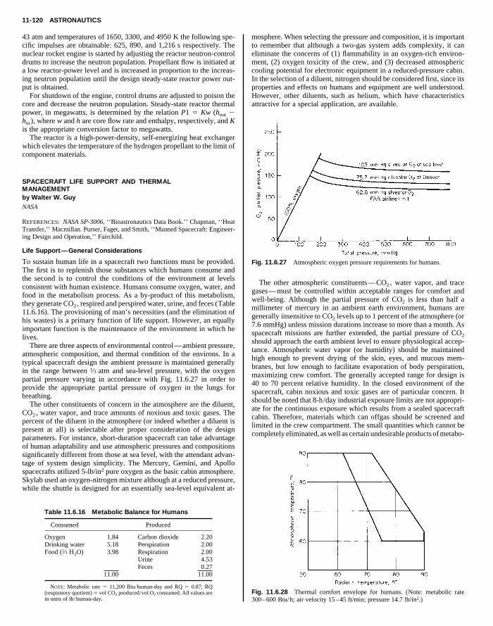
11-120 ASTRONAUTICS
43 atm and temperatures of 1650, 3300, and 4950 K the following spe-cific impulses are obtainable: 625, 890, and 1,216 s respectively. Thenuclear rocket engine is started by adjusting the reactor neutron-controldrums to increase the neutron population. Propellant flow is initiated ata low reactor-power level and is increased in proportion to the increas-ing neutron population until the design steady-state reactor power out-put is obtained.
For shutdown of the engine, control drums are adjusted to poison thecore and decrease the neutron population. Steady-state reactor thermalpower, in megawatts, is determined by the relation P1 5 Kw (hout 2
mosphere. When selecting the pressure and composition, it is importantto remember that although a two-gas system adds complexity, it caneliminate the concerns of (1) flammability in an oxygen-rich environ-ment, (2) oxygen toxicity of the crew, and (3) decreased atmosphericcooling potential for electronic equipment in a reduced-pressure cabin.In the selection of a diluent, nitrogen should be considered first, since itsproperties and effects on humans and equipment are well understood.However, other diluents, such as helium, which have characteristicsattractive for a special application, are available.
Copyright (C) 1999 by The McGraw-Hill Companies, Inc. All rights reserved. Use ofthis product is subject to the terms of its License Agreement. Click here to view.
hin ), where w and h are core flow rate and enthalpy, respectively, and Kis the appropriate conversion factor to megawatts.
The reactor is a high-power-density, self-energizing heat exchangerwhich elevates the temperature of the hydrogen propellant to the limit ofcomponent materials.
SPACECRAFT LIFE SUPPORT AND THERMALMANAGEMENTby Walter W. GuyNASA
REFERENCES: NASA SP-3006, ‘‘Bioastronautics Data Book.’’ Chapman, ‘‘HeatTransfer,’’ Macmillan. Purser, Faget, and Smith, ‘‘Manned Spacecraft: Engineer-ing Design and Operation,’’ Fairchild.
Life Support—General Considerations
To sustain human life in a spacecraft two functions must be provided.The first is to replenish those substances which humans consume andthe second is to control the conditions of the environment at levelsconsistent with human existence. Humans consume oxygen, water, andfood in the metabolism process. As a by-product of this metabolism,they generate CO2, respired and perspired water, urine, and feces (Table11.6.16). The provisioning of man’s necessities (and the elimination ofhis wastes) is a primary function of life support. However, an equallyimportant function is the maintenance of the environment in which helives.
There are three aspects of environmental control—ambient pressure,atmospheric composition, and thermal condition of the environs. In atypical spacecraft design the ambient pressure is maintained generallyin the range between 1⁄3 atm and sea-level pressure, with the oxygenpartial pressure varying in accordance with Fig. 11.6.27 in order toprovide the appropriate partial pressure of oxygen in the lungs forbreathing.
The other constituents of concern in the atmosphere are the diluent,CO2, water vapor, and trace amounts of noxious and toxic gases. Thepercent of the diluent in the atmosphere (or indeed whether a diluent ispresent at all) is selectable after proper consideration of the designparameters. For instance, short-duration spacecraft can take advantageof human adaptability and use atmospheric pressures and compositionssignificantly different from those at sea level, with the attendant advan-tage of system design simplicity. The Mercury, Gemini, and Apollospacecrafts utilized 5-lb/in2 pure oxygen as the basic cabin atmosphere.Skylab used an oxygen-nitrogen mixture although at a reduced pressure,while the shuttle is designed for an essentially sea-level equivalent at-
Table 11.6.16 Metabolic Balance for Humans
Consumed Produced
Oxygen 1.84 Carbon dioxide 2.20Drinking water 5.18 Perspiration 2.00Food (2⁄3 H2O) 3.98 Respiration 2.00
Urine 4.53Feces 0.27
11.00 11.00
NOTE: Metabolic rate 5 11,200 Btu/human-day and RQ 5 0.87; RQ(respiratory quotient) 5 vol CO2 produced/vol O2 consumed. All values arein units of lb/human-day.
Fig. 11.6.27 Atmospheric oxygen pressure requirements for humans.
The other atmospheric constituents—CO2, water vapor, and tracegases—must be controlled within acceptable ranges for comfort andwell-being. Although the partial pressure of CO2 is less than half amillimeter of mercury in an ambient earth environment, humans aregenerally insensitive to CO2 levels up to 1 percent of the atmosphere (or7.6 mmHg) unless mission durations increase to more than a month. Asspacecraft missions are further extended, the partial pressure of CO2
should approach the earth ambient level to ensure physiological accep-tance. Atmospheric water vapor (or humidity) should be maintainedhigh enough to prevent drying of the skin, eyes, and mucous mem-branes, but low enough to facilitate evaporation of body perspiration,maximizing crew comfort. The generally accepted range for design is40 to 70 percent relative humidity. In the closed environment of thespacecraft, cabin noxious and toxic gases are of particular concern. Itshould be noted that 8-h/day industrial exposure limits are not appropri-ate for the continuous exposure which results from a sealed spacecraftcabin. Therefore, materials which can offgas should be screened andlimited in the crew compartment. The small quantities which cannot becompletely eliminated, as well as certain undesirable products of metabo-
Fig. 11.6.28 Thermal comfort envelope for humans. (Note: metabolic rate300–600 Btu/h; air velocity 15–45 ft/min; pressure 14.7 lb/in2.)

SPACECRAFT LIFE SUPPORT AND THERMAL MANAGEMENT 11-121
lism, must be actively removed by the life-support system to maintainan acceptable atmosphere for the crew.
The third of the environmental control aspects—atmospheric ther-mal condition—is subject to several design variables, all of which mustbe taken into account. Thermal comfort is a function of the temperatureand relative humidity of the surrounding atmosphere, the velocity ofany ventilation present, and the temperature and radiant properties ofthe cabin walls and equipment. The interrelationship of these parame-ters is shown in Fig. 11.6.28 for a reasonable range of flight clothingensembles. Because of the effective insulations available to the vehicle
electrochemical means. This process is mechanically simple (as com-pared to the adsorption-desorption system) but does require more elec-trical power. However, it has an integration advantage in that it providesthe CO2 collected from the atmosphere mixed with hydrogen, whichmakes its effluent a natural feedstock for either one of several CO2
reduction subsystems (which will be required for oxygen recovery on aspace station). Although Figure 11.6.29 identifies the various life-sup-port subsystem choices for candidate spacecraft designs of differentmission durations, this information should be used only as a guide. Thecrew size as well as other design parameters can skew the range of
Copyright (C) 1999 by The McGraw-Hill Companies, Inc. All rights reserved. Use ofthis product is subject to the terms of its License Agreement. Click here to view.
designers, the problem of thermal control in the spacecraft cabin isgenerally one of heat removal. Utilizing increased ventilation rates toenhance local film coefficients is one means of improving thermal com-fort within the cabin. However, the higher power penalties associatedwith gas circulation blowers, as compared to liquid pumps, should sug-gest using the spacecraft thermal control liquid circuit in reducing thetemperature of the radiant environment as potentially a lower-poweralternative. However, if the walls or equipment are chilled below thedew point, condensation will occur.
As an additional benefit, maintaining an acceptable thermal environ-ment through radiative means reduces the psychological annoyance of adrafty, noisy environment. Ventilation rates between 15 and 45 ft /minare generally considered comfortable, and exceeding this range shouldbe avoided.
Life Support—Subsystems Selection
In designing the life-support system for a spacecraft, subsystems con-cepts must be selected to accomplish each of the required functions.This process of selection involves many design criteria. Size, weight,power consumption, reliability of operation, process efficiency, serviceand maintenance requirements, logistics dependency, and environmen-tal sensitivity may each be very important or inconsequential dependingon the spacecraft application. In general, for life support subsystems,the dominant selection criterion is mission duration. Various subsystemchoices for accomplishing the life support functions are shown in Fig.11.6.29.
To illustrate the relationship between mission duration and subsys-tem selection, the various concepts for removal of CO2 from the atmo-sphere shown in Fig. 11.6.29b will be discussed. The simplest methodof controlling the level of CO2 in the spacecraft cabin is merely to purgea small amount of the cabin atmosphere overboard. This concept issimple and reliable and requires almost no subsystem hardware, al-though it does incur a fairly significant penalty for atmospheric makeup.For missions such as Alan Sheppard’s first Mercury flight, this conceptis probably optimum. However, even a minor increase in mission dura-tion will result in a sizable weight penalty to the spacecraft. By adding asimple chemical absorption bed to the spacecraft ventilation loop (witha chemical such as lithium hydroxide as the absorbent), the expendablepenalty for CO2 removal can be reduced to the weight of the chemicalcanisters consumed in the absorption process. This concept was used onthe Apollo spacecraft. The penalty for this type of concept also becomesprohibitive if mission durations are further extended. For missions suchas Skylab, the expendable chemical absorbent can be replaced by aregenerable adsorbent. This change eliminates the lithium hydroxideweight penalty but incurs a small atmospheric ullage loss during thevacuum regeneration of the adsorbent. In addition, the regenerable sys-tem is more complex, requiring redundant beds (one for adsorptionwhile the alternate bed desorbs), and mechanical-timing circuits andswitching valves. This result is typical in that reducing expendable re-quirements is generally at the expense of system complexity.
The three CO2 removal concepts discussed above all prevent thesubsequent use of the collected CO2 after removal from the atmosphere.Should the CO2 be required for reclaiming the metabolic oxygen (suchas will be the case for a space station design), the regenerable conceptscan be adapted to accommodate retrieval of the CO2 during desorption.However, this enhancement further complicates the subsystem design.There is an alternative CO2 removal concept available which utilizes afuel-cell-type reaction to concentrate the CO2 in the atmosphere through
applicability for each subsystem (e.g., a large crew can render expend-able dependent subsystems inappropriate even for relatively short mis-sions).
Fig. 11.6.29 Concepts to accomplish the life-support function. (a) Water re-covery; (b) atmospheric revitalization.
There is another major aspect of life support system design for space-craft (in addition to subsystem selection) and that is process integrationand mass balance. For example, a space-station-class life-support sys-tem design must accommodate wastewater with a wide range of con-tamination levels—from humidity condensate which includes onlyminor airborne contamination to various wash and rinse waters (includ-ing personal hygiene, shower, clothes washing, and dish washing) andurine. The degree of contamination generally influences the reclamationprocess selection; therefore, multiple contaminated sources tend to re-sult in multiple subsystem processes. For example, highly contaminatedwater, such as urine, is most reliably reclaimed through a distillationprocess since evaporation and condensation can be more effectivelyutilized to separate dissolved and particulate material from the water,while less contaminated wash waters can be effectively reclaimedthrough osmotic and mechanical filtration techniques at significantlyless power penalties in watts / lb H2O recovered. Regardless of the tech-

11-122 ASTRONAUTICS
Fig. 11.6.30 Life-support systems mass balance. (All values are in pounds per day for an eight-person crew.)
niques selected, water must be made available for drinking, food prepa-ration, and cleaning the crew and the equipment they use, as well as forgenerating the oxygen they breathe. In fact, the space station life-sup-port design process can be looked upon, in one respect, as a multifacetedwater balance since the dissociation of CO2 and generation of O2 bothinvolve water in the respective processes. Figure 11.6.30 is a typicalspace station schematic depicting the interrelationship of the subsys-tems and the resulting mass balance.
Thermal Management—General
transport efficiency and low-temperature characteristics. The thermaltransport efficiency is important since the size, weight, and power re-quirements of the pumping and distribution system depend on this pa-rameter. However, in the environs of deep space the potential exists forvery low temperatures. Therefore, for maximum system operating flex-ibility, the characteristics of the thermal transport fluid must be suchthat operation of the system can continue even in a cold environment;thus, low-temperature properties become a fluid selection constraint.Although the range of acceptable fluids is broader here, several fluids inthe Freon family meet these requirements. For single-phase, pumped-
Copyright (C) 1999 by The McGraw-Hill Companies, Inc. All rights reserved. Use ofthis product is subject to the terms of its License Agreement. Click here to view.
Considerations
Although there is an aspect of life support associated with thermal com-fort, the area of spacecraft thermal management encompasses a muchbroader scope. In the context of this section, thermal management in-cludes the acquisition and transport of waste heat from the varioussources on the spacecraft, and the disbursing of this thermal energy atvehicle locations requiring it, as well as the final rejection of the netwaste heat to space. Although there are thermal implications to thedesign of most spacecraft hardware, the Life Support and ThermalManagement section only deals with the integration of the residual ther-mal requirements of the various vehicle subsystems to provide anenergy-efficient spacecraft design (i.e., one which utilizes wasteheat to the maximum and therefore minimizes requirements for thevehicle heat rejection system).
Thermal management systems are typically divided into two parts.The first, associated with the spacecraft cabin, has design requirementsassociated with maintaining the crew environment and equipment lo-cated in the cabin at acceptable temperatures, and in addition has specialrequirements imposed on its design because of the location of the sys-tem in the pressurized compartment and its proximity to humans. Theseadditional requirements are usually dominant. Any cooling mediumwhich is used in the crew compartment must have acceptable toxicolog-ical and flammability characteristics in order to not impose a hazard tothe crew in the event of malfunction or leakage. Although there arethermal control fluids which have low toxicity potential, reasonableflammability characteristics and adequate thermal transport properties,none are better than water.
The second aspect of the thermal management system involves thosespacecraft systems located outside the cabin. The dominant design cri-teria in thermal control fluid selection for these systems are thermal
fluid systems, the temperature levels of the heat sources are important indetermining the optimum sequence for locating equipment in the ther-mal circuit. The equipment with the lowest-temperature heat sink re-quirements are accommodated by placing them immediately after theheat rejection devices, while equipment which can accept a higher-temperature heat sink are located downstream. Also, those subsystemswhich require heating must be located at a point in the circuit which canprovide the thermal energy at the required temperature level.
Typically spacecraft heat sources include cabin-atmosphere heat ex-changers, the avionics system as well as other electronic black boxes,power generation and storage equipment, etc., while heat sinks includepropulsion system components, various mechanical equipment requir-ing intermittent operation, dormant fluid systems which have freezingpotential, etc. The ultimate elimination of the net thermal energy (i.e.,sources minus sinks) is by rejection to space. This is accomplishedthrough expendables or radiation.
Recent developments in thermal management technology have re-sulted in the consideration of a two-phase acquisition, transport, andrejection system. This concept uses the heat of evaporation and conden-sation of the transport fluid to acquire and reject thermal energy, reduc-ing by several orders of magnitude the amount of fluid required to bepumped to the various heat sources and sinks within the spacecraft. Thisconcept has the added advantage of operating nearly isothermally, per-mitting the idea of a thermal ‘‘bus’’ to be included in future spacecraftdesign, with indiscriminate sequencing of the heat sources and sinkswithin the vehicle.
Thermal Management Subsystem Selection
The subsystem selection process associated with the thermal manage-ment area depends largely on the magnitude of thermal energy being

SPACECRAFT LIFE SUPPORT AND THERMAL MANAGEMENT 11-123
Fig. 11.6.31 Range of application of various heat-rejection methods.
managed and the duration of the mission. Figure 11.6.31 graphicallydepicts the areas of applicability for various types of heat-rejectiondevices as a function of these parameters.
Small heat-rejection requirements can sometimes be met by directheat sinking to the structure (or a fluid reservoir). Often, passive heatsinks need to be supplemented with fusible heat sinks (to take advantageof the latent heat of fusion) or evaporative heat sinks (to take advantageof the latent heat of evaporation). Of the three types of heat sinks, theevaporative heat sink is the only one which has been used as the primaryvehicle heat-rejection device in the manned spaceflight program to date.
fully used integral skin radiators, the unique characteristics of the outersurface of the orbiter required a different technique be adopted for itsradiator design. Accordingly, the radiators were designed to be de-ployed from inside of the payload bay doors. This not only providesgood exposure to space, but also, in the case of the forward panels,allows two-sided exposure of the panels, thereby doubling the activeradiating area.
Heat rejected Qrej, according to the Stefan-Boltzmann law, is givenby the following equation:
Copyright (C) 1999 by The McGraw-Hill Companies, Inc. All rights reserved. Use ofthis product is subject to the terms of its License Agreement. Click here to view.
Both the Mercury spacecraft and the lunar module utilized a waterevaporative heat sink in this manner. However, the Apollo spacecraftand the shuttle have also used evaporative heat sinks and Skylab used afusible heat sink as supplemental heat rejection devices.
Since space is the ultimate heat sink for any nonexpendable heatrejection, devices which allow the thermal energy which has been col-lected in spacecraft coolant circuits to be radiated to space become themainstay of the thermal management system. These ‘‘radiators’’ takemany forms. The simplest design involves routing the cooling circuitsto the external skin of the spacecraft so that the thermal energy can beradiated to deep space. Because of spacecraft configuration restrictions,only partial use can be made of the external skin of the spacecraft, andthe amount of thermal energy which can be rejected by this technique isthereby limited. Although the Gemini and Apollo spacecraft success-
Fig. 11.6.32 Space radiator energy balance.
Qrej 5 «gAT4
where g 5 constant, 0.174 3 1028 Btu/(h ? ft2 ? *R4); « 5 emittanceproperty of surface (termed emissivity), A 5 area available for radia-tion; and T 5 radiating temperature. From this equation it is obviousthat a radiator with both sides exposed will reject twice as much heat tospace as one of the same dimensions which is integral with the skin ofthe vehicle. A space radiator can absorb as well as reject thermal energy.The net heat rejected Qnet from a radiator is given by the followingequation:
Qnet 5 Qrej 2 OA51
N
Qabs
The energy absorbed by the radiator, Qabs , can come from varioussources (see Fig. 11.6.32).

11-124 ASTRONAUTICS
The most common heat sources for an earth-orbiting spacecraft aredirect solar impingement, reflected solar energy from the earth (i.e.,albedo), direct radiation from the earth, radiation from other parts of thespacecraft, and radiation from other spacecraft in the immediate vicin-ity. These energy sources are absorbed on the radiator surface in directproportion to the absorptance characteristic of the surface, termed ab-sorptivity. Emissivity and absorptivity are unique to each surface mate-rial but are variables directly linked to the temperature of the source ofthe radiation (i.e., wavelength of the radiation). Therefore, since ab-sorptivity and emissivity are characteristics of the surface, the careful
tors which have been used on spacecraft to date. Because of this advan-tage, future missions which require either of the three types of radiators(i.e., integral skin, deployable, or space constructible) will utilize theheat pipe concept to transport the thermal energy to the exposed radiat-ing surface.
The design of space radiators can take many forms, but the basicconcept is an exposed surface made of a conducting material with regu-larly spaced fluid tubes to distribute the heat over the surface (see Fig.11.6.34).
Copyright (C) 1999 by The McGraw-Hill Companies, Inc. All rights reserved. Use ofthis product is subject to the terms of its License Agreement. Click here to view.
selection of a surface coating can significantly enhance the effective-ness of the radiator. The coating should have a high emissivity in thewavelength of the rejected energy from the radiator (for good radiationefficiency) and a low absorptivity in the wavelength of the impingingradiation (for minimal absorbed energy). Since generally the earth andthe surrounding spacecraft are producing thermal energy of essentiallythe same wavelength as the radiator, it is necessary to restrict the viewof the radiating surface to these objects since absorptivity and emissiv-ity of a surface are equal for the same wavelength energy. Thus, radia-tors which can be located so that they are not obstructed from viewingdeep space by elements of the spacecraft or other spacecraft in thevicinity will be much more effective in rejecting waste heat. The sun,however, emits thermal energy of a dramatically different wavelengthand, therefore, coatings can be selected which absorb less than 10 per-cent of the solar energy while radiating nearly 90 percent of the energyat the emitting temperature of the radiator.
For applications which require large radiating surface areas as com-pared to the vehicle’s size, integral skin radiators offer insufficient areaand thus space radiators which use deployment schemes must be con-sidered. However, as radiators become larger the mechanisms becomevery complicated. To circumvent the mechanical problems of deploy-ment, a new radiator concept has been developed which allows in-orbitconstruction. This concept utilizes a single-tube heat pipe as the primaryelement (see Fig. 11.6.33).
Fig. 11.6.33 Basic heat-pipe operation.
There are two distinct advantages of heat pipe radiators. The first isthat assembly of large surface areas in-orbit can be effected withoutbreaking into the thermal control circuit. This is practical since the heatpipe radiator element is completely self-contained. The second advan-tage is that in-orbit damage from accidental collision or meteoroidpuncture affects only that portion of the radiator actually damaged anddoes not drain the entire radiating surface of fluid as it would the radia-
Fig. 11.6.34 Typical radiator tube/fin configurations.
The selection of the material and configuration of the radiating sur-face (i.e., honeycomb, box structure, thin sheet, etc.) determine its ther-mal conductance. This conductance, when coupled with tube spacingand the internal heat transfer characteristics within the tube and fluidsystem, determines the temperature gradient on the radiating surface
Tube diameter
Radiator
Total weight
Rad
iato
r w
eigh
t
Optimum
Tube weight
Tube spacing (constant flow)Fin thickness (constant area)
Fin weight
Largetubes
Smalltubes
Tube spacing
Fin thickness
Fig. 11.6.35 Radiator configuration optimization.

DOCKING OF TWO FREE-FLYING SPACECRAFT 11-125
between adjacent tubes. This so-called ‘‘fin effectiveness’’ represents aloss in radiating potential for any particular radiator design; therefore,these parameters should be selected carefully to optimize the radiatordesign within the constraints of each application. Figure 11.6.35 dem-onstrates the effect of the configuration parameters of the radiator onpanel weight.
DOCKING OF TWO FREE-FLYING SPACECRAFT
increases. As the vehicles interact the mechanism interfaces are indexedinto alignment as the system responds to the impact loads. The compli-ance of the system occurs in two forms: mechanism movement and rigidbody vehicle motion.
When the docking interfaces interact, the system responds in sixdegrees of freedom and the docking system is stroked as the mechanismabsorbs the relative misalignments. Once the interfaces are fullyaligned, capture latches lock the opposing interfaces together, and thevehicles are ‘‘soft-docked.’’ After capture, residual energy in the sys-tem allows relative motion between the structures to continue. Depend-
Copyright (C) 1999 by The McGraw-Hill Companies, Inc. All rights reserved. Use ofthis product is subject to the terms of its License Agreement. Click here to view.
by Siamak Ghofranian and Matthew S. SchmidtRockwell Aerospace
REFERENCES: Ghofranian, Schmidt, Briscoe, and Shliesing, ‘‘Space ShuttleDocking to MIR, Mission-1’’; Ghofranian, Schmidt, Briscoe, and Shliesing,‘‘Simulation of Shuttle /MIR Docking’’; Ghofranian, Schmidt, Lin, Khalessi, andRazi, ‘‘Probabilistic Analysis of Docking Mechanism Induced Loads for MIR/Shuttle Mission’’; 35th Structures, Structural Dynamics, and Materials Conf.AIAA/ASME/ASCE/AHS/ASC. Haug, ‘‘Computer Aided Kinematics and Dy-namics of Mechanical Systems,’’ vol 1: ‘‘Basic Methods,’’ Allyn and Bacon.Greenwood, ‘‘Principles of Dynamics,’’ Prentice-Hall.
The information in this section covers the mechanics of docking twofree-flying unconstrained vehicles in space. Different methods of mat-ing are addressed with the emphasis applied to docking. The contentdoes not encompass all facets of the procedure, but it does bring forththe physics of the operation which make the process an engineeringchallenge.
Types of Mating
The understanding of mating is a precursor to preliminary design. Dif-ferent techniques of mating free-flying bodies are often discussed whenplanning the rendezvous of two vehicles in space. The mating of twostructures can be performed in three ways: docking, berthing or a com-bination of both. Docking relies on the transfer of vehicle momentum toprovide the means to force the docking ports into alignment. If a signifi-cant amount of momentum is required for capture, jet firings can beused to introduce the impulse into the system as needed. Berthing relieson a secondary system, such as a robotic arm to enforce the dockingports into alignment. The active vehicle grapples the other with a robotmanipulator and guides the structural interfaces together. If manipulatorusage is attempted, specific design factors need to be considered: armconfiguration, gearbox stiffness, linkage flexibility, and controllability.
Mating of two structures in space is by every means considered amultibody dynamic event. Docking involves a significant level of mo-mentum transfer, while berthing involves relatively little. The dynamicsresult from the deliberate impact of the two vehicles. As docking occursthe system responds with rigid-body motion and mechanical motion ofthe docking device. Depending on the relative states between the vehi-cles and the mode in which the maneuver is attempted, the response ofthe system and the physics vary considerably.
For discussion purposes the two docking vehicles can be consideredas a target vehicle (passive) and a docking vehicle (active). The passivevehicle maintains attitude control as the active vehicle is navigatedalong an approach corridor. The active vehicle holds an attitude controlmode with translational control authority. As the corridor narrows,sighting aids, range, and range-rate feedback on both vehicles are usedto guide the docking ports into contact.
As the vehicles approach, a closing velocity exists. From a designstandpoint the operation of a docking system involves various mecha-nism operational phases: mechanism deployment, interface contact andcapture, attenuation of relative motion, mechanism retraction, andstructural lockup. The deployment phase is where the mechanism isdriven from its stowed position to its ready-to-dock position. Vehicleinterface contact and capture are initiated when the docking ports ofeach vehicle are maneuvered into contact. Ideally, a positive closingvelocity should be maintained from initial contact through capture.Once an opening velocity develops, the probability of a failed capture
ing on the location of the docking system relative to the vehicle centerof masses, the motion may dissipate due to the inherent hysteresis in thedocking system; otherwise, separate energy-dissipation devices may benecessary. After attenuation the vehicles are likely to be misaligned dueto the new relative equilibrium position of the spacecraft. Separate pro-cedures or devices can be used to bring the structural interfaces intoalignment.
The retraction process is where the active mechanism is driven backto its stowed position. Once they are fully retracted, the structural inter-faces are latched at hard interfaces, and the vehicles are ‘‘hard-docked.’’
The mass of each vehicle is an essential part of the docking systemdesign. The momentum of the docking vehicle is the medium whichprovides the force required by the docking mechanism to comply withthe relative misalignments between the vehicles at the docking inter-face. The operation can be complicated if a vehicle center of mass isoffset from the longitudinal axis of the docking system. As a result, thevehicle effective mass at the docking interface is reduced. Furthermore,the center of mass offset induces relative rotation after contact whichcomplicates the capture and attenuation process. Ideally two vehiclesshould dock such that the velocity vector and longitudinal axis of thedocking system have minimum offset from the center of mass. Therelative rotation of the vehicles after contact is known as jackknifing.
The docking mechanism center-of-mass offset and the vehicle sizesignificantly influence the design of the docking interfaces, attenuationcomponents, docking aids, piloting procedures, and capture-assistmethods. The relative vehicle misalignments and rates at the momentthe docking interfaces first come into contact (initial conditions) shouldbe known in order to size the mechanism attenuation components, toestablish piloting procedures and training criteria, and to study the me-chanics of the system before, during, and after docking.
The initial conditions result from vehicle as-built tolerances, thermaland dynamic distortions, variation in piloting performance, and controlsystem tolerances. The misalignments are composed of lateral mis-alignments in the plane of the docking interface and angular misalign-ments about thee axes. The rates are composed of translational veloci-ties along three axes and angular velocities about three axes.
The mass and motion of the system are the basic ingredients forproviding the energy necessary to join the interfaces. Ideally theinterfaces should capture before an opening velocity develops betweenthe docking interfaces. Adequate momentum at the docking port is re-quired to actuate the mechanism. The impulse introduced to the systemduring the impact must be less than that required to reduce the relativeinterface velocity to zero. If the relative interface velocity goes to zerobefore capture, the vehicles will separate. For low closing velocities, asmall axial impulse due to initial contact can reduce the relative inter-face velocity to zero and cause a ‘‘no capture’’ condition.
A drive system along the longitudinal axis of the docking mechanismor reaction control jets increases the probability of capture. It extendsthe docking system toward the target vehicle once initial contact ismade and thus improves capture performance for a docking vehicle witha low closing velocity. However, a drawback of a drive system is thatthe reaction has the tendency to push the vehicles apart. The action of jetthrusting has the opposite effect; it tends to push the vehicles together. Ifthe momentum required to provide a low possibility of no capture be-comes operationally prohibitive, thrusting can be used as a substituteand applied as necessary.

11-126 PIPELINE TRANSMISSION
As energy introduced into the system increases, whether in the formof vehicle momentum or jets pulsing, a tradeoff exists between accept-able internal vehicle loads, allowable component stroke limits, vehiclejackknifing, and piloting capability.
Vehicle Mass and Inertia Effects
Concentrated spherical masses colliding in two dimensions can be usedto describe the dynamic effects of an impact. The same class of exam-ples are consistently used in beginning physics textbooks to describe themacroscopic concepts of impulse, momentum, and energy. The same
unknown parameter becomes the work required to bring the system torest.
Design Parameters
The energy loss during docking is equal to the work done, F 3 d, by themechanism-attenuation components. If a hysteresis brake is used tobring the system to rest, then a trade can be performed on the force-distance relationship by using
1⁄2Meffy2 5 Fd
vid
Copyright (C) 1999 by The McGraw-Hill Companies, Inc. All rights reserved. Use ofthis product is subject to the terms of its License Agreement. Click here to view.
theory should be applied to understand the requirements of mating twovehicles and perform conceptual and preliminary design studies.A single-degree-of-freedom mechanical equivalent exhibiting sim-ple harmonic motion is a useful example for understanding the me-chanics.
Consider two spacecraft in a two-dimensional plane on a plannedcourse of docking without any misalignments and with some closingvelocity. If only the docking-axis degree of freedom is considered, theeffective mass of each body, M1 and M2 , can be computed from
M1 (or M2) 5 M 2 (ML)2/(I 1 ML2)
where M is the vehicle mass, I is the vehicle mass moment of inertiaabout the center of mass, and L is the mass center offset from thedocking axis. In this case the process of capture and attenuation can bethought of as a perfectly plastic impact of two bodies. The masses dockand stick together. After impact the two bodies continue their trajectorywith some final velocity. The combined effective mass of the twobodies represented as a single degree of freedom can be computed fromMeff 5 M1M2 /(M1 1 M2). Since momentum is conserved during a per-fectly plastic impact, kinetic energy loss during docking can be com-puted from 1⁄2Meffy2, where y is the capture velocity. Since at capturewe know the effective mass of the system and the capture velocity, the
11.7 PIPELINEby G. Da
REFERENCES: AGA publication ‘‘Gas Facts.’’ Huntington, ‘‘Natural Gas andGasoline,’’ McGraw-Hill. Leeston, Crichton, Jacobs, ‘‘The Dynamic Natural Gas
Industry,’’ University of Oklahoma Press. Lester, Hydraulics for Pipeliners, Oil-dom. Bell, ‘‘Petroleum Transportation Handbook,’’ McGraw-Hill. Bureau ofMines, ‘‘Mineral Yearbook,’’ Vol. II, Fuels. ‘‘The Transportation of Solids inSteel Pipelines,’’ Colorado School of Mines Research Foundation, Inc. Echter-hoff, ‘‘Pipeline Economics Revisited,’’ PCGA, 1981. Petroleum Supply Monthly,Department of Energy, Energy Information AdmFebruary 1994. ‘‘US Interstate Pipelines Begin 1993Journal, Nov. 22, 1993.where F represents the force necessary to bring the system to rest overdistance d. Using the hysteresis brake as a starting point provides theaverage about which other devices would oscillate. For an underdampedspring/damper attenuation system, the relative motion and maximumforce can be computed from
x 5 y /vd 3 e2zv sin vd t and F 5 Kx 1 C dx /dt
respectively. In this representation,
vd 5 v(1 2 z2)1/2 and v2 5 K/Meff
where z represents the damping factor and K and C represent the attenu-ation component characteristics. As can be seen, minimal knowledge ofthe basic system characteristics can be used to design the type andarrangement of the attenuation components. During the design of theattenuation components the following components may prove useful:preloaded centering springs, staged springs, ON/OFF dampers, andvariable-level hysteresis brakes. The material in this section is only afirst look at understanding the design of a docking system. As moredetail is developed, the effects of relative vehicle motion, interface con-tact dynamics, mechanism performance, and vehicle flexibility need tobe simulated, which goes beyond the scope of this section. For a com-prehensive background, the reader should refer to the cited references.
TRANSMISSIONBounds
are now restricted from including costs for these activities with the costsof buying, transporting, and selling gas, due to the mandate that gather-
ing be provided as a separate service. The swing in market demand hasmagnified the need for storage facilities in both gathering and marketareas to provide the flexibility required to operate efficiently in anopen-access market. Open-access marketing has replaced bundled salestaneous needs of buyers at competitive prices.ing was first tried in the early 1980s, compet-curtailment of gas flow to approximately
through a national pipeline grid that had
inistration, March 1993–on Upbeat,’’ Oil and Gas
services to meet the instanWhen open-access marketitive bidding resulted in18 trillion ft3 per year
NATURAL GAS
General According to AGA Estimates for 1991, approximately 65percent of the U.S. natural-gas reserves occur in seven states (Texas,New Mexico, Oklahoma, Louisiana, Wyoming, Alaska, and Kansas)and only about 40 percent of the total natural gas produced there isconsumed within those states. Within these seven states alone, esti-mated production in 1991 exceeded 16.6 trillion ft3 (472.6 billion m3).Total exports, interstate and international, from these states in 1991were estimated at approximately 13.1 trillion ft3 (371.8 billion m3),while imports were approximately 4.5 trillion ft3 (127.4 billion m3).Offshore production is becoming increasingly significant. In 1991, ap-proximately 18 percent of the total proven U.S. natural-gas reserveswere located offshore.
Implementation of FERC Order 636 has had a significant impact onnatural-gas transmission pipelines. Pipeline companies which built andoperated gathering systems as needed to support contractual obligations
moved 24 trillion ft3 per year in the 1970s. Hubs are now being estab-lished to provide access to natural gas capacity release so that pipelinecapacity may be more effectively utilized than ever before. Electronicbulletin boards (EBBs) are being refined to operate on an ever-expand-ing information superhighway to provide open access to gas suppliesand markets.
The need to transport natural gas from the producing regions to con-suming areas throughout the country has generated a burgeoning net-work of transmission pipelines. In 1950, there were 314,000 mi(505,000 km) of gas pipelines in this country. By 1991, with natural gassupplying 24 percent of the nation’s energy requirements, this mileagehad increased to 1,225,000 mi (1,972,000 km), an increase of 390 per-cent in 40 years. Between the years of 1984 and 1986, the total length ofgas transmission pipeline in the United States declined by 2,500 mi(4,000 km). The significant drop in demand for pipeline steel pushedmany domestic pipe mills into insolvency. Other pipe mills specializedin production of a single type of longitudinal seam, such as seamless

NATURAL GAS 11-127
(SMLS), double-submerged arc weld (DSAW), or electric resistanceweld (ERW) pipe. Domestic pipeline installation rebounded in 1987,with the installation of approximately 2,800 mi (4,500 km) of large-dia-meter steel pipeline.
Modern gas pipelines consist of all diameters from 2 in to 42 in in allgrades of specified minimum yield strengths (SMYS) from 35,000 to70,000 lb/in2. The type of longitudinal seams available are SMLS insizes ranging from 2 in to 20 in, ERW in sizes ranging from 2 in to 24 in,and DSAW in sizes ranging from 16 in to 42 in. Higher yield strengthsare usually more cost-effective in sizes larger than 10 in.
valves, gas measurement, by either AGA dimensioned orifice(s) or byturbine meters, and flow control valves. Overpressure protection mayalso be required. If a large temperature drop is anticipated across any ofthe pressure-reducing valves, then a radiant heater or indirect-firedheater may be required. A rough estimate of temperature drop is 7°F per100 lb/in2 of pressure drop. Electronic flow measurement has becomecommonplace, meeting the requirements of current regulations. Micro-processors calculate, remotely monitor, and control flow in real timeusing the latest calculation methods of the AGA and American Petro-leum Institute (API) reports. The quality of the gas is also measured by
Copyright (C) 1999 by The McGraw-Hill Companies, Inc. All rights reserved. Use ofthis product is subject to the terms of its License Agreement. Click here to view.
Although the trend has been toward the use of larger pipe diametersand pipe steel of greater tensile strength, the economics of pipe produc-tion and coating and the ease of handling, including transportation aswell as installation, has led to greater utilization of 36-in-diameter(0.91-m) pipe with a specified minimum yield strength of 65,000 lb/in2
(4,570 kg/cm2). In 1992, 36-in-diameter pipe accounted for approxi-mately 36 percent of the total steel used in construction of large trans-mission pipelines. Although significant mileage of 42-in-diameter(1.07-m) pipeline has been placed in gas service, no new 42-in-diameterpipeline construction was recorded by the American Gas Association(AGA) in 1992.
Main line valves are usually ball or gate and are of the full-openingvariety to allow for the passage of cleaning pigs and inspection tools.Ball, gate, and plug valves are installed on piping other than main linepiping.
Pipe bends are usually made on site by a contractor; however, onshort-distance pipelines, or in cases where a large degree of bend isrequired, shop-fabricated bends are produced by induction heating.
Repairs to a pipeline segment according to current regulations of theDepartment of Transportation (DOT) are to either replace the segment,or use welded steel sleeves. A new method currently being tested byboth the DOT and industry is a polymer composite reinforcement wrap(Clock Spring) which is wrapped around the repair area. For this type ofrepair, welding is not required.
The rapidly growing network of large diameter pipelines, along withincreasing pressure capabilities, has brought forth a considerable rise inprime mover and compressor requirements. Natural-gas pipelines in theUnited States have experienced an increase from about 6 million in-stalled hp (4.5 million kW) in 1960 to 14 million hp (10.6 million kW)by the end of 1991, an increase of 233 percent in 30 years. Natural-gasengines, natural-gas turbines, and electric motors are most generallyemployed as prime movers on gas pipelines. The gas engines generallydrive reciprocating compressors; gas turbines and electric-motor driversare usually connected to centrifugal compressors. The industry trend istoward the use of larger, centrifugal compressor units because of theinherent economic advantages. Prime movers in general use have in-creased in size from the early 1950s to the early 1990s as follows: gasengines from 2,500 to 13,500 hp (1,865 to 10,070 kW), gas turbinesfrom 1,000 to 50,000 hp (745 to 37,310 kW), and electric-motor driversfrom 2,500 to 20,000 hp (1,865 to 14,920 kW). Modified aircraft-typejet engines are also employed as prime movers driving centrifugal com-pressors and range from 800 to 50,000 hp (600 to 37,310 kW).
Much progress has been made in automated operations of all types ofpipelines. Valves, measuring and regulating stations, and other facilitiesare operated remotely or automatically. Factory-packaged compressor-station assemblies, most of which are highly automated, are now com-monplace. Whole compressor stations with thousands of horsepowerare operated unattended by the use of coded dispatching systems han-dled by high-speed communications.
Automatic supervision and operation of pipeline systems are becom-ing almost commonplace in today’s climate of microprocessor-basedremote terminal units (RTUs). These ultra-high-speed data-gatheringsystems can be used to gather operational data, do calculations, provideproportional integral derivative (PID) process control, and undertakeother auxiliary functions. Data may be communicated to a central dis-patch office for real-time control. A system of several hundred locationsmay be scanned and reported out in a few seconds.
Natural gas measurement stations usually consist of pressure control
one of several means. For small-volume stations a continuous gassampler accumulates a small volume for laboratory testing. Mediumvolume stations will use a sampler and/or a gravitometer, while large-volume stations will use a gas chromatograph.
Flow From the thermodynamic energy balance equations for theflow of compressible fluids (Sec. 4), the general flow formula is derivedand expressed in BuMines Monograph 6 (1935) as
Q 5 KT0
P0F(P2
1 2 P22)d5
GTf LfG1/2
(11.7.1)
where Q is the rate of flow, ft3/day; T0 is the temperature base, °R; P0 isthe pressure base, psia; P1 is the initial gas pressure, psia; P2 is the finalgas pressure, psia; d is the internal pipe diameter, in; G is the specificgravity of the gas, which is dimensionless (for air, G 5 1.0); Tf is the gasflowing temperature, °R; and Lf is the length of the pipeline, mi. Thegeneral flow equation for constant-volume (steady-state), isothermal,horizontal flow of natural gas is given by U.S. BuMines Monograph 9(1956) as
Q 5 38.7744Tb
PbF(P2
1 2 P22)D5
f ZGTLG0.5
(11.7.2)
where Q 5 rate of flow, ft3/day; Tb 5 temperature base, °R; Pb 5pressure base, psia; P1 5 inlet pressure, psia; P2 5 outlet pressure, psia;D 5 internal pipe diameter, in; f 5 friction factor, dimensionless; Z 5average gas compressibility, dimensionless; G 5 gas gravity (for air,G 5 1.00); T 5 average flowing temperature, °R; L 5 length of pipe,mi. Monograph 9 also gives a good discussion of friction factors and ele-vation corrections.
Other flow equations may be derived from the general equation bysubstitution of the proper expression for the friction factor. This appliesto the Panhandle A equation which has the form
Q 5 435.87STb
PbD1.0788S P2
1 2 P22
G0.8539TLD0.5394
D2.6182E (11.7.3)
where E 5 pipeline flow efficiency, a dimensionless decimal fraction(design values of 0.88 to 0.96 are common). In the Panhandle A equa-tion, the compressibility is included in the pipeline efficiency, and theother symbols are as previously defined. This formula may be solvedgraphically as described by C. W. Marvin, Oil and Gas Journal, Sept.20, 1954.
An AGA paper, Steady Flow in Gas Pipelines (1965), gives a goodgeneral review of constant-volume gas flow equations, both with andwithout elevation corrections. Equations and test data are included forboth the partially turbulent (Reynolds number dependent) flow regimeand the fully turbulent flow regime using effective internal pipe rough-ness. In this reference the drag factor is introduced to account for pres-sure losses for fittings such as bends and valves and is applied in thepartially turbulent flow regime.
When the volume of gas flowing varies with time and position (tran-sient or unsteady-state flow), the simultaneous momentum and massbalance equations are usually solved by use of numerical methods andwith the aid of computers. An AGA computer program, Pipetran, isavailable for this purpose, as are several related texts on transient flow.A paper entitled Gas Transportation System Modeling appears in the1972 AGA Operating Proceedings. Gas flowing in a pipeline undergoesa number of transient, or unsteady-state, flow conditions caused by suchthings as prime movers starting and stopping, valves opening and clos-

11-128 PIPELINE TRANSMISSION
ing, and flows either into or out of the pipeline. DOS-based computerprograms, such as TransFlow (Gregg Engineering) and GASUS(Stoner & Associates) and others, allow the engineer to model simple aswell as complex pipeline situations. These programs can be used to testproposed system expansions such as loops or additional compressorstations, to perform capacity studies, and to evaluate the effects of thetransients mentioned above.
Compression The theoretical horsepower requirements for a sta-tion compressing natural gas may be calculated by polytropic compres-sion formulas (see Sec. 4). The change of state that takes place in almost
ment Committee Report 3 of the AGA provide supplemental designguidelines. The equation for pipeline design pressure, as dictated by theDOT in Part 192 of Title 49, Code of Federal Regulations, is
P 52St
DFET (11.7.6)
where P 5 design pressure, psig; S 5 specified minimum yieldstrength, lb/in2, t 5 nominal wall thickness, in; D 5 nominal outside
Copyright (C) 1999 by The McGraw-Hill Companies, Inc. All rights reserved. Use ofthis product is subject to the terms of its License Agreement. Click here to view.
all reciprocating compressors is close to polytropic. Heat of compres-sion is taken away by the jacket cooling and by radiation, and a smallamount of heat is added by piston-ring friction. Compression by centrif-ugal compressors in even closer to polytropic (see Sec. 14).
For general design, the horsepower requirements for a station com-pressing natural gas with reciprocating compressors can be calculated asfollows:
Reciprocating station horsepower 5 hpZs
Ts
520(11.7.4)
The value for hp can be taken from Fig. 11.7.1, typical manufac-turer’s curve; Ts is suction temperature, °R; and Zs can be taken fromFig. 11.7.2.
Fig. 11.7.1 Reciprocating-compressor horsepower (MW) graph. Rc 5P2 /P1 5 discharge pressure, lb/in2 abs 4 suction pressure, lb/in2 abs.
Similarly, the horsepower requirements for a station compress-ing natural gas with centrifugal compressors can be calculated asfollows:
Centrifugal station horsepower 5hpZs
Ec
Ts
520(11.7.5)
The value for hp can be taken from Fig. 11.7.3, typical centrifugalhorsepower curve; Ec is the centrifugal-compressor shaft efficiency.(Design shaft efficiencies of 80 to 85 percent are common.)
Compression ratios across a single machine normally do not exceed3.0 because of outlet temperature limitations. For greater ratios, com-pressors can be arranged in series operation with an interstage gascooler placed between the individual units. Multiple units can also beplaced in parallel operation in order to increase flexibility and providefor routine maintenance.
Design The pipe and fittings for gas transmission lines are manu-factured in accordance with the specifications of the API, ANSI,ASTM, and MSS (see also Sec. 8). Interstate pipelines are installed andoperated in conformance with regulations of the U.S. Department ofTransportation (DOT). The ANSI B31.8 Code and the Gas Measure-
Fig. 11.7.2 Supercompressibility factor Z for natural gas. (Natural gas, 1 per-cent N2.)
diameter, in; F 5 design factor based on population density in the areathrough which the line passes, dimensionless; E 5 longitudinal jointfactor, dimensionless; and T 5 temperature derating factor (appliesabove 250°F only), dimensionless. For offshore lines and cross-countrypipelines in areas where the population density is very low, the factor Fis 0.72. For seamless, double-submerged arc weld or electric resistanceweld pipe with an E value of 1.00 and an operating temperature below250°F in these low-population density areas, the equation can be written
P 5 1.44St/D (11.7.7)
The selection of the diameter, steel strength, and wall thickness of aline and the determination of the optimum station spacing and sizing are
Fig. 11.7.3 Centrifugal-compressor horsepower (MW) graph. Rc 5P2 /P1 5 discharge pressure, lb/in2 abs 4 suction pressure, lb/in2 abs.

CRUDE OIL AND OIL PRODUCTS 11-129
Fig. 11.7.4 Schematic relationship of cost of transportation versus design capacity for a given length of line withvarious pipeline diameters at equal design pressures.
based on transportation economics. Figures 11.7.4 through 11.7.6 showschematically methods of analysis commonly used to relate design fac-tors to the cost of transportation. A perspective of various elements ofthe cost of transportation for a long-distance, large-diameter, fully de-veloped pipeline system is presented in Fig. 11.7.7.
The cost of installed pipelines varies greatly with the location, thetype of terrain, the design pressure, the total length to be constructed,and many other factors. In general, figures from $23,000 to $38,000 perinch (per 2.54 cm) of OD represent the range of approximate costs permile (per 1.61 km) of installed pipeline. Offshore pipeline installed
CRUDE OIL AND OIL PRODUCTS
General Approximately 91 percent of the U.S. proven liquid hydro-carbon reserves are situated in the seven states of Alaska, California,Louisiana, New Mexico, Oklahoma, Texas, and Wyoming or in themarine areas off their coasts. Offshore production is becoming increas-ingly significant. The refinement of multiphase pumping systems hasenhanced crude oil recovery from formerly marginal offshore fields. In1991, approximately 11 percent of the total proven crude oil reserveswere located in federal waters offshore of California, Louisiana, and
Copyright (C) 1999 by The McGraw-Hill Companies, Inc. All rights reserved. Use ofthis product is subject to the terms of its License Agreement. Click here to view.
costs vary with such items as length, water depth, bottom conditions,pipeline crossings, depth of bury, and many other factors. These costsrange from $38,000 to $54,000 per inch (per 2.54 cm) of OD per mile(per 1.61 km) for a typical offshore pipeline. Compressor-station in-stalled costs vary widely with the amount and type of horsepower to beinstalled and with the location, the type of construction, and weatherconditions. The installed costs of gas-turbine stations range from $900to $1,600 per installed hp ($1,206 to $2,145 per kW); gas-engine sta-tions, from $1,000 to $1,800 per hp ($1,340 to $2,413 per kW); andelectric-motor stations, from $600 to $1,500 per hp ($800 to $2,000per kW).
After a pipeline system is constructed and fully utilized, expansion ofdelivery capacity can be accomplished by adding pipeline loops (con-necting segments of line parallel to the original line), by adding addi-tional horsepower at compressor stations, or by a combination of thesetwo methods.
Texas. The major markets in which petroleum products are consumedare remote from the proven reserves. About one-half of all petroleumconsumed in the United States is imported and must be moved fromports to the centers of consumption. Eighty-nine percent of all move-ments of petroleum and petroleum products is made by pipelines. Theinterstate pipelines alone transport over 11.4 billion bbl (1.82 billionm3) of petroleum a year. There are about 163,000 mi (262,300 km) ofoperating interstate liquid-petroleum trunk lines in the United States.
Centrifugal pumps have been used extensively. Generally, these unitsare multistaged, installed in series or parallel, depending on the applica-tion. Many operators install smaller multiple units instead of largersingle units to improve operating efficiency and flexibility.
Reciprocating pumps are installed in parallel; i.e., a common suctionand a common discharge header are utilized by all pumps. There areinstances where rotary, gear, and vane-type pumps have been employedto fulfill specific requirements.

Fig. 11.7.5 Schematic relationship of cost of transportation versus pipeline steel strength and wall thickness.A 5 30 in 3 0.312 in, WT 3 52,000 lb/in2 min. yield (779-lb/in2 operating pressure).B 5 30 in 3 0.344 in, WT 3 56,000 lb/in2 min. yield (923-lb/in2 operating pressure).C 5 30 in 3 0.350 in, WT 3 60,000 lb/in2 min. yield (1,008-lb/in2 operating pressure).D 5 30 in 3 0.385 in, WT 3 65,000 lb/in2 min. yield (1,200-lb/in2 operating pressure).
Fig. 11.7.6 Schematic relationship of cost of transportation versus design capacity for a given pipeline diameter andlength, with various spacings of compressor stations.
11-130
Copyright (C) 1999 by The McGraw-Hill Companies, Inc. All rights reserved. Use ofthis product is subject to the terms of its License Agreement. Click here to view.

SOLIDS 11-131
Table 11.7.1
Pump-station Cost per installed hpinstalled hp, total (1hp 5 0.746 kW)
250–500 $760–800500–750 $560–600750–1,000 $440–480
1,000–2,000 $310–350Above 2,000 $275
Copyright (C) 1999 by The McGraw-Hill Companies, Inc. All rights reserved. Use ofthis product is subject to the terms of its License Agreement. Click here to view.
Fig. 11.7.7 Analysis of (a) investment and (b) cost of transportation.
Electrically driven centrifugal pumps are now widely employed forthe liquid pipeline industry because they are environmentally friendlyand because of their compactness, low initial costs, and ease of control.Centrifugal pumps driven by gas-turbine engines have also come intoroutine use.
Positive-displacement and turbine meters are in general use on prod-ucts systems (see Sec. 16). Totalizers for multimeter installations andremote transmission of readings are an industry standard. Greater appli-cation of meters with crude-oil gathering facilities is being made asautomatic-custody units are installed.
Flow The Darcy formula,
hf 5 f LV 2/D2g (11.7.8)
where hf 5 friction loss, ft; f 5 friction factor (empirical values), di-mensionless; L 5 length of pipe, ft; D 5 ID, ft; V 5 velocity flow, ft/s;and g 5 32.2 ft /s2, is in general use by engineers making crude-oilpipeline calculations. The Darcy formula, when stated in a form utiliz-ing conventional pipeline units, is
P 5 34.87f B2S/d5 (11.7.9)
where P 5 friction press drop, lb/(in2 ? mi); f 5 friction factor (empiri-cal values), dimensionless; B 5 flow rate, bbl /h (42 gal /bbl); S 5specific gravity of the oil, dimensionless; d 5 ID, in.
The Williams and Hazen formula, which has wide acceptance for prod-uct pipeline calculations, can be stated in a form employing conven-tional pipeline terms as follows:
P 52340B1.852S
C 1.852d4.870(11.7.10)
where P 5 friction press drop, lb/in2 per 1,000 ft of pipe length; B 5flow rate, bbl /h; S 5 specific gravity of the oil product; C 5 frictionfactor, dimensionless; and d 5 ID, in. The friction factor C includes theeffect of viscosity and differs with each product (C for gasoline is 150;for no. 2 furnace oil, 130; for kerosene, 134).
The brake horsepower for pumping oil is RSh/3960E or BP/2450E,where R 5 flow rate, gal/min; S 5 specific gravity of the oil; h 5 pumphead, ft; E 5 pump efficiency, decimal fraction; B 5 flow rate, bbl /h;and P 5 pump differential pressure, lb/in2.
Design The pipe and fittings for oil transmission lines are manufac-tured in accordance with specifications of the API and are fabricated,installed, and operated in the United States in conformance with FederalRegulations, DOT, Part 195 (see also Sec. 8). Many factors influencethe working pressure of an oil line, and the ANSI B31.4 code for pres-sure piping is used as a guide in these matters. A study of the hydraulicgradient, land profile, and static-head conditions is made in conjunctionwith the selection of the main-line pipe (Sec. 3).
Determining the pipe size and station spacing to transport a given oilor oil product at a specified rate of flow and to provide the lowest cost oftransportation is a complex matter. Usually the basic approach is toprepare (1) a series of pipeline cost estimates covering a range of pipediameters and wall thicknesses and (2) a series of station cost estimatesfor evaluation of the effect of station spacing. By applying capitalcharges to the system cost estimates and estimating the system operat-ing costs, a series of transportation-cost curves similar to those in Fig.11.7.8 can be drawn.
Estimates of $20,000 to $40,000 per in (per 2.54 cm) of OD representthe cost per mile (1.61 km) of installed trunk pipeline. The tabulation ofpump-station investment costs for automated electric-motor, centrifu-gal-type installations presented in Table 11.7.1 can be used for prelimi-nary evaluations.
Careful design and good operating practice must be followed to mini-mize contamination due to interface mixing in oil-product pipelines.When the throughput capacity of an oil line becomes fully utilized, addi-tional capacity can be obtained by installing a parallel pipeline or a par-tial-loop line. A partial loop is a parallel line which runs for only part ofthe distance between stations. In the case of product lines, care-ful attention must be paid to the design of the facilities where the loop lineis tied into the original pipeline to prevent commingling of products.
SOLIDS
General Solids may be transported by pipeline by a number of dif-ferent methods. In capsule pipelining, dry solids are placed in a circularcapsule which is then pumped down the pipeline. This method can haveeconomic and other advantages in many cases, especially where wateris scarce, because the water is never contaminated and can be returnedeasily in a closed loop.
Another method being developed for the transport of coal is by coallogs. Pulverized coal is mixed with a binder (usually petroleum-based)to form a solid log, designed to resist water absorption, that can betransported down the pipeline intact. No dewatering is required withthis method of coal transportation and because the binder is combustibleit enhances burning.
The most prevalent method of transporting solids by pipeline is byslurry. A slurry is formed by mixing the solid in pulverized form with atrue liquid, usually water, to a consistency which can be pumped downthe pipeline as a liquid. Nonvolatile gases, such as carbon dioxide, may
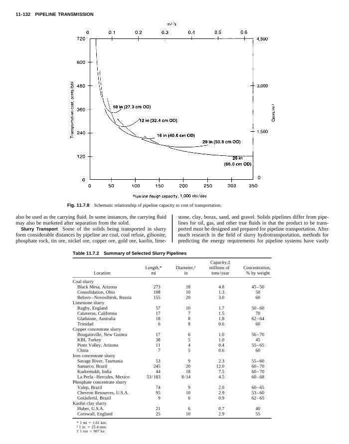
11-132 PIPELINE TRANSMISSION
Fig. 11.7.8 Schematic relationship of pipeline capacity to cost of transportation.
also be used as the carrying fluid. In some instances, the carrying fluidmay also be marketed after separation from the solid.
Slurry Transport Some of the solids being transported in slurryform considerable distances by pipeline are coal, coal refuse, gilsonite,phosphate rock, tin ore, nickel ore, copper ore, gold ore, kaolin, lime-
stone, clay, borax, sand, and gravel. Solids pipelines differ from pipe-lines for oil, gas, and other true fluids in that the product to be trans-ported must be designed and prepared for pipeline transportation. Aftermuch research in the field of slurry hydrotransportation, methods forpredicting the energy requirements for pipeline systems have vastly
Table 11.7.2 Summary of Selected Slurry Pipelines
Capacity,‡Length,* Diameter,† millions of Concentration,
Location mi in tons/year % by weight
Copyright (C) 1999 by The McGraw-Hill Companies, Inc. All rights reserved. Use ofthis product is subject to the terms of its License Agreement. Click here to view.
Coal slurryBlack Mesa, Arizona 273Consolidation, Ohio 108Belovo–Novosibirsk, Russia 155
Limestone slurry
Rugby, England 57Calaveras, California 17Gladstone, Australia 18Trinidad 6Copper concentrate slurryBougainville, New Guinea 17KBI, Turkey 38Pinto Valley, Arizona 11China 7
Iron concentrate slurrySavage River, Tasmania 53Samarco, Brazil 245Kudremukh, India 44La Perla–Hercules, Mexico 53/183
Phosphate concentrate slurryValep, Brazil 74Chevron Resources, U.S.A. 95Goiasfertil, Brazil 9
Kaolin clay slurryHuber, U.S.A. 21Cornwall, England 25
* 1 mi 5 1.61 km.† 1 in 5 25.4 mm.‡ 1 ton 5 907 kg.
18 4.8 45–5010 1.3 5020 3.0 60
10 1.7 50–607 1.5 708 1.8 62–648 0.6 60
6 1.0 56–705 1.0 454 0.4 55–655 0.6 60
9 2.3 55–6020 12.0 60–7018 7.5 60–70
8/14 4.5 60–68
9 2.0 60–6510 2.9 53–606 0.9 62–65
6 0.7 4010 2.9 55

SOLIDS 11-133
Fig. 11.7.9 System relative transportation cost for various main-line pipe sizes.
improved and slurries are transported today at much higher concentra-tions than 10 years ago. In the early 1980s, slurry designs ranging from45 to 58 percent concentration, by weight, were common. Today, ultra-fine coal-water mixtures with concentrations, by weight, ranging up to75 percent, or more, are used. Dispersants and chemical additives, suchas Carbogel and Densecoal are used to reduce drag and facilitatepumping. These additives significantly reduce the operating costs ofslurry pipelines. Additional savings are realized by direct burning ofthese high-concentration coal-water mixtures through a nozzle, sincedewatering is not required.
for other forms of transportation since drying can be eliminated after thecleaning operation.
Coal-slurry preparation normally consists of a wet grinding processfor reducing clean coal to the proper particle size and size-range distri-bution. The final slurry-water concentration can be adjusted before itenters the pipeline with quality control of the slurry holding tanks. Thecost of slurry preparation is only slightly affected by changes in concen-tration or size consist. The normal slurry-preparation-plant practice is tohold the concentration within 1 percent of design to provide a slurrywith a uniform pressure drop. Continued research has made it possible
Copyright (C) 1999 by The McGraw-Hill Companies, Inc. All rights reserved. Use ofthis product is subject to the terms of its License Agreement. Click here to view.
Current trends in the construction of solids pipelines and those pro-posed for construction indicate that future transportation of mineralsand other commodities will bear more consideration. Some of the com-mercially successful slurry pipelines throughout the world are listed inTable 11.7.2.
Advances in slurry rheology studies and technology related to homo-geneous and heterogeneous slurry transport have made the potential ofslurry pipelining unlimited. Immediate advantages for slurry pipelinesexist where the solids to be transported are remotely located; however,each potential slurry transport project possesses some other advantages.Materials must satisfy the following conditions to be transported bylong-distance pipelines: (1) the largest particle size must be limited tothat which can readily pass through commercially available pumps,pipes, and other equipment; (2) solids must mix and separate easilyfrom the carrying fluids or be consumable in the slurry state; (3) mate-rial degradation must be negligible or beneficial to pipelining and utili-zation; (4) material must not react with the carrying fluid or becomecontaminated in the pipeline; (5) the solids-liquid mixture must not beexcessively corrosive to pipe, pumps, and equipment; (6) solidsmust not be so abrasive as to cause excessive wear at carrying veloci-ties.
Coal Slurry Uncleaned coal can be transported by pipeline, but amore stable and economic long-distance pipeline operation can beachieved with clean coal. The use of clean coal allows a variety ofsupply sources; produces a slurry with a lower, more uniform friction-head loss; reduces the pipe-wall wear; and increases the system capac-ity. Cleaning pipeline coal costs considerably less than cleaning coals
to predict accurately the anticipated pressure drop in a pipeline by usinga laboratory and computer correlation.
Optimum characteristics for a slurry are (1) maximum concentration,(2) low rate of settling, and (3) minimum friction-head loss. Variableswhich can be manipulated to control and optimize slurry design areparticle shape, size distribution, concentration, and ash content. Estab-lished computer techniques are used to evaluate these variables.
Design Because of the many slurry variations, there is no singleformula available by which the friction-head loss can be readily deter-mined for all slurry applications. A general approach is described byWasp, Thompson, and Snoek (The Era of Slurry Pipelines, Chemtech.,Sept. 1971, pp. 552-562), and by Wasp, Kenny, and Gandhi in theirbook, ‘‘Solid-Liquid Flow Slurry Pipeline Transportation,’’ giving cal-culation methods which have been developed for predicting slurry pres-sure drops. The described methods are quite accurate and can be usedfor preliminary design. Additional calculation procedures and methodsfor specifying slurry size consist (solid size-range distribution) and ve-locity have been developed by continuing research and may be found inthe following books: Shook and Roco, ‘‘Slurry Flow Principles andPractice,’’ Butterworth Heinemann, 1991, and Wilson, Addie, and Clift,‘‘Slurry Transport Using Centrifugal Pumps,’’ Elsevier, 1992. Slurryhydraulics should be verified with bench-scale tests and compared withcommercial operating data reference points or pilot-plant operationsbefore constructing a full-scale long-distance pipeline.
Slurry velocities are generally limited to a minimum critical velocityto prevent solids from settling to the bottom of the pipe and a maximumvelocity to prevent excessive friction-head loss and pipe-wall wear.

11-134 CONTAINERIZATION
These velocity limitations and the throughput volume determine thediameter of the mainline pipe. The relationship of volume and velocityto the pipe diameter is expressed as ID 5 0.6392 √(gal /min)/V, wherethe ID is in inches, gal /min is the volume rate of slurry flow (gallons perminute), and V is flow velocity, ft /s.
Pipe-wall thickness in inches is computed by the modified Barlowformula as [(PD/2SF) 1 tc ]/tm , where P 5 maximum pressure, lb/in2;D 5 pipe OD, in; S 5 minimum yield strength of the pipe, lb/in2; F 5safety factor; tm 5 pipe mill tolerance, usually 0.875; and tc 5 internalerosion/corrosion allowances, in, for the life of the system. The internal
Q 5 maximum flow rate through the station in gallons per min-ute, and 1,716 is a constant, gal /(ft ? in2). Stations usually employpositive-displacement reciprocating pumps of the type used for oil-fieldmud pumps, as they attain high pressures with low slurry velocities.This allows fewer stations and lower overall costs than with centrif-ugal pumps. Stations are located where the friction-head loss andthe effects of terrain have reduced the pressure head to 100 ft(30.48 m). Centrifugal pump usage is advantageous in low-pressure,high-velocity applications such as coarse coal transportation for shortdistances.
INnt
Copyright (C) 1999 by The McGraw-Hill Companies, Inc. All rights reserved. Use ofthis product is subject to the terms of its License Agreement. Click here to view.
metal loss results from the erosion of corrosion products from the pipewall and thus can be limited with chemical inhibitors and velocity con-trol. This metal loss occurs in all pipeline steels and according toCowper, Thompson, et al., Processing Steps: Keys to SuccessfulSlurry-Pipeline Systems, Chem. Eng., Feb. 7, 1972, pp. 58–67, must beevaluated on a case-by-case basis. A minimum pipe wall of 0.250 in(0.635 cm) is often used to provide mechanical strength for large lineseven where pressures and wear permit the use of a thinner wall. Coalpipelines employ a graduated wall thickness to meet the demands of thehydraulic gradient, which saves pipe costs.
Pump-station hydraulic horsepower is calculated as (Pd 2 Ps )(Q)/1,716 where (Pd 2 Ps ) 5 pressure rise across the station lb/in2,
11.8 CONTA(Staff Co
REFERENCE: Muller, ‘‘Intermodal Freight Transportation,’’ 2d ed., Eno Founda-
tion for Transportation.Shipping of freight has always suffered from pilferage and other lossesassociated with the handling of cargo and its repeated exposure toweather conditions and to human access. In addition, the extremelylabor-intensive loading and unloading practices of the past becamemore and more expensive. In the late 1920s and erunners of present-day container service were offercontainers on trucks to services in which railroad c
The annual tonnage throughput for any diameter line can be variedwithin the velocity limits or by intermittent operation near the low ve-locity limit. The optimum main-line size for high-load-factor systems isfound by comparing the relative cost of transportation for a series ofpipe sizes, as in Fig. 11.7.9.
When a main-line size is selected, the cost of transportation for thatline size at various rates of throughput is weighed against the projectedsystem growth and compared with other line sizes to determine the sizewhich gives the best overall system economics. Coal pipelines cannotbe expanded by line looping because of the velocity limitations. Someexpansion can be attained by oversizing the line and operating it inter-mittently near the minimum velocity in the earlier years of life.
ERIZATIONribution)
be stacked up to six units high. Since containers are designed with
oceangoing shipment in mind where the container, and those stacked ontop of it, will be rising and falling with the movement of the ship, theadditional acceleration forces have to be taken into account. This isusually done by rating the maximum stacking load using a g forceof 1.8.typical 20-ft container. At each of the eightfittings which facilitate the lifting, stacking,
g down of units. These fittings have specially
arly 1930s the fore-ed. They varied fromars were loaded onto
Figure 11.8.1 shows acorners there are specialinterconnecting, and tyin
shaped slots and holes which enable standard crane and sling hooks andrubber-tired trailers and delivered to the customer’s door with no inter-mediate handling of the cargo. Starting in 1956, containerization as weknow it today came into being.
The immense savings in shipping costs resulted in the rapid growth ofcontainerization throughout the world in the 1960s and 1970s and ininternational standardization. The time savings obtainable through theuse of containers is particularly noticeable in maritime service. It isestimated that a container-handling ship can achieve a 4 : 1 sea-to-porttime ratio compared to 1 : 1 for a conventional break-bulk ship.
CONTAINER SPECIFICATIONS
There are many standards which apply to containers, among which areISO, ANSI, the International Container Bureau (BIC), and the Ameri-can Bureau of Shipping (ABS).
Types Ninety percent of containers are dry, nonrefrigerated unitswith double doors on one end. Other types include refrigerated and/orinsulated units, ventilated units, tank containers, and frames with fold-ing ends or corner posts for carrying large items such as automobiles.
Condensation can be a problem inside a closed container. While agood unit can protect against outside elements, it cannot protect againstcondensation inside the container unless special steps are taken. Con-densation typically arises from the moisture in the product beingshipped; temperature changes during the trip; or moisture from dun-nage, packing, or the container itself.
Construction materials usually consist of a steel, aluminum, or fiber-glass outer cover on an internal steel frame. Containers are designed to
clevises to be used as well as special hooks and twist-locks.Sizes The most widely used containers are 20 ft (6.1 m) or 40 ft
(12.2 m) long by 8 ft (2.5 m) wide by 8 ft (2.5 m) high. The usualheight of 102 in (2.6 m) includes an 8-in-deep (200-mm) underframe.This frame often has two, or sometimes four, transverse slots for forkliftforks. Standard lengths are: 20, 35, 40, 45, and 48 ft (6.1, 10.7, 12.2,13.7, and 14.6 m).
Typical specifications for a 20-ft (6.1-m) container are: maximumgross weight of 52,910 lb (24,000 kg), tare of 5,070 lb (2,300 kg), pay-load of 47,840 lb (21,700 kg), cubic capacity of 1,171 ft3 (33.2 m3), andallowable stacked weight for a g force of 1.8 of 423,280 lb(192,000 kg).
Typical specifications for a 40-ft (12.2-m) container are: maximumgross weight of 67,200 lb (30,480 kg), tare of 8,223 lb (3,730 kg), pay-load of 58,977 lb (26,750 kg), allowable stacked weight for a g force of1.8 of 304,170 lb (182,880 kg), cubic capacity of 2,300 ft3 (65 m3).Thus a 40-ft (12.2-m) container has roughly the same volume as a 40-ft(12.2-m) highway semitrailer. A typical 40-ft (12.2-m) dry-cargocontainer with an aluminum outer skin weighs about 6,000 lb(2,720 kg).
Specifications for a typical 40-ft (12.2-m) refrigerated container are:maximum gross weight of 67,200 lb (30,480 kg), tare of 8,770 lb(3,980 kg), payload of 58,430 lb (26,500 kg), allowable stacked weightfor a g force of 1.8 of 423,307 lb (192,000 kg), cubic capacity of2,076 ft3 (58.8 m3). The refrigeration system specifications are: mini-mum inside temperature of 0°F (2 18°C), maximum outside tempera-ture of 100°F (38°C). The refrigeration system is powered through
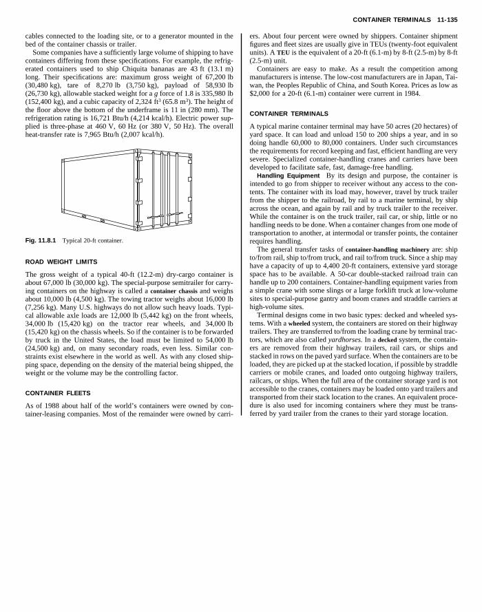
CONTAINER TERMINALS 11-135
cables connected to the loading site, or to a generator mounted in thebed of the container chassis or trailer.
Some companies have a sufficiently large volume of shipping to havecontainers differing from these specifications. For example, the refrig-erated containers used to ship Chiquita bananas are 43 ft (13.1 m)long. Their specifications are: maximum gross weight of 67,200 lb(30,480 kg), tare of 8,270 lb (3,750 kg), payload of 58,930 lb(26,730 kg), allowable stacked weight for a g force of 1.8 is 335,980 lb(152,400 kg), and a cubic capacity of 2,324 ft3 (65.8 m3). The height ofthe floor above the bottom of the underframe is 11 in (280 mm). The
ers. About four percent were owned by shippers. Container shipmentfigures and fleet sizes are usually give in TEUs (twenty-foot equivalentunits). A TEU is the equivalent of a 20-ft (6.1-m) by 8-ft (2.5-m) by 8-ft(2.5-m) unit.
Containers are easy to make. As a result the competition amongmanufacturers is intense. The low-cost manufacturers are in Japan, Tai-wan, the Peoples Republic of China, and South Korea. Prices as low as$2,000 for a 20-ft (6.1-m) container were current in 1984.
Copyright (C) 1999 by The McGraw-Hill Companies, Inc. All rights reserved. Use ofthis product is subject to the terms of its License Agreement. Click here to view.
refrigeration rating is 16,721 Btu/h (4,214 kcal/h). Electric power sup-plied is three-phase at 460 V, 60 Hz (or 380 V, 50 Hz). The overallheat-transfer rate is 7,965 Btu/h (2,007 kcal/h).
Fig. 11.8.1 Typical 20-ft container.
ROAD WEIGHT LIMITS
The gross weight of a typical 40-ft (12.2-m) dry-cargo container isabout 67,000 lb (30,000 kg). The special-purpose semitrailer for carry-ing containers on the highway is called a container chassis and weighsabout 10,000 lb (4,500 kg). The towing tractor weighs about 16,000 lb(7,256 kg). Many U.S. highways do not allow such heavy loads. Typi-cal allowable axle loads are 12,000 lb (5,442 kg) on the front wheels,34,000 lb (15,420 kg) on the tractor rear wheels, and 34,000 lb(15,420 kg) on the chassis wheels. So if the container is to be forwardedby truck in the United States, the load must be limited to 54,000 lb(24,500 kg) and, on many secondary roads, even less. Similar con-straints exist elsewhere in the world as well. As with any closed ship-ping space, depending on the density of the material being shipped, theweight or the volume may be the controlling factor.
CONTAINER FLEETS
As of 1988 about half of the world’s containers were owned by con-tainer-leasing companies. Most of the remainder were owned by carri-
CONTAINER TERMINALS
A typical marine container terminal may have 50 acres (20 hectares) ofyard space. It can load and unload 150 to 200 ships a year, and in sodoing handle 60,000 to 80,000 containers. Under such circumstancesthe requirements for record keeping and fast, efficient handling are verysevere. Specialized container-handling cranes and carriers have beendeveloped to facilitate safe, fast, damage-free handling.
Handling Equipment By its design and purpose, the container isintended to go from shipper to receiver without any access to the con-tents. The container with its load may, however, travel by truck trailerfrom the shipper to the railroad, by rail to a marine terminal, by shipacross the ocean, and again by rail and by truck trailer to the receiver.While the container is on the truck trailer, rail car, or ship, little or nohandling needs to be done. When a container changes from one mode oftransportation to another, at intermodal or transfer points, the containerrequires handling.
The general transfer tasks of container-handling machinery are: shipto/from rail, ship to/from truck, and rail to/from truck. Since a ship mayhave a capacity of up to 4,400 20-ft containers, extensive yard storagespace has to be available. A 50-car double-stacked railroad train canhandle up to 200 containers. Container-handling equipment varies froma simple crane with some slings or a large forklift truck at low-volumesites to special-purpose gantry and boom cranes and straddle carriers athigh-volume sites.
Terminal designs come in two basic types: decked and wheeled sys-tems. With a wheeled system, the containers are stored on their highwaytrailers. They are transferred to/from the loading crane by terminal trac-tors, which are also called yardhorses. In a decked system, the contain-ers are removed from their highway trailers, rail cars, or ships andstacked in rows on the paved yard surface. When the containers are to beloaded, they are picked up at the stacked location, if possible by straddlecarriers or mobile cranes, and loaded onto outgoing highway trailers,railcars, or ships. When the full area of the container storage yard is notaccessible to the cranes, containers may be loaded onto yard trailers andtransported from their stack location to the cranes. An equivalent proce-dure is also used for incoming containers where they must be trans-ferred by yard trailer from the cranes to their yard storage location.