TraPHic: Trajectory Prediction in Dense and Heterogeneous Traffic Using

Weighted Interactions

Rohan Chandra

University of Maryland

College Park

Uttaran Bhattacharya

University of Maryland

College Park

Aniket Bera

University of North Carolina

Chapel Hill

Dinesh Manocha

University of Maryland

College Park

https://go.umd.edu/TraPHic

Abstract

We present a new algorithm for predicting the near-term

trajectories of road agents in dense traffic videos. Our ap-

proach is designed for heterogeneous traffic, where the road

agents may correspond to buses, cars, scooters, bi-cycles,

or pedestrians. We model the interactions between different

road agents using a novel LSTM-CNN hybrid network for

trajectory prediction. In particular, we take into account

heterogeneous interactions that implicitly account for the

varying shapes, dynamics, and behaviors of different road

agents. In addition, we model horizon-based interactions

which are used to implicitly model the driving behavior of

each road agent. We evaluate the performance of our pre-

diction algorithm, TraPHic, on the standard datasets and

also introduce a new dense, heterogeneous traffic dataset

corresponding to urban Asian videos and agent trajecto-

ries. We outperform state-of-the-art methods on dense traf-

fic datasets by 30%.

1. Introduction

The increasing availability of cameras and computer vi-

sion techniques has made it possible to track traffic road

agents in realtime. These road agents may correspond to

vehicles such as cars, buses, or scooters as well as pedes-

trians, bicycles, or animals. The trajectories of road agents

extracted from a video can be used to model traffic patterns,

driver behaviors, that are useful for autonomous driving. In

addition to tracking, it is also important to predict the fu-

ture trajectory of each road agent in realtime. The predicted

trajectories are useful for performing safe autonomous nav-

igation, traffic forecasting, vehicle routing, and congestion

management [32, 11].

In this paper, we deal with dense traffic composed of het-

Figure 1. Trajectory Prediction: in dense heterogeneous traf-

fic conditions. The scene consists of cars, scooters, motorcycles,

three-wheelers, and bicycles in close proximity. Our algorithm

(TraPHic) can predict the trajectory (red) of each road-agent close

to the ground truth (green) and is better than other prior algorithms

(shown in other colors).

erogeneous road agents. The heterogeneity corresponds to

the interactions between different types of road agents such

as cars, buses, pedestrians, two-wheelers (scooters and mo-

torcycles), three-wheelers (rickshaws), animals, etc. These

agents have different shapes, dynamic constraints, and be-

haviors. The traffic density corresponds to the number of

distinct road agents captured in a single frame of the video

or the number of agents per unit length (e.g., a kilometer)

of the roadway. High density traffic is described as traffic

with more than 100 road agents per Km. Finally, an interac-

tion corresponds to how two road agents in close proximity

affect each other’s movement or avoid collisions.

There is considerable work on trajectory prediction for

moving agents [2, 18, 36, 12, 26, 30, 12, 26]. Most of

these algorithms have been developed for scenarios with

single type of agents (a.k.a. homogeneous agents), which

may correspond to human pedestrians in a crowd or cars

18483

driving on a highway. Furthermore, many prior methods

have been evaluated on traffic videos corresponding to rel-

atively sparse scenarios with only a few heterogeneous in-

teractions, such as the NGSIM [1] and KITTI [15] datasets.

In these cases, the interaction between agents can be mod-

eled using well-known models based on social forces [19],

velocity obstacles [35], or LTA [31].

Prior prediction algorithms do not work well on dense,

heterogeneous traffic scenarios because they do not model

the interactions accurately. For example, the dynamics

of a bus-pedestrian interaction differs significantly from a

pedestrian-pedestrian or a car-pedestrian interaction due to

the differences in shape, size, maneuverability, and veloci-

ties. The differences in the dynamic characteristics of road

agents affect their trajectories and how they navigate around

each other in dense traffic situations [29]. Moreover, prior

learning-based prediction algorithms typically model the in-

teractions uniformly for all other road agents in its neigh-

borhood and the resulting model assigns equal weight to

each interaction. This method works well for homogeneous

traffic. However, i does not work well for dense hetero-

geneous traffic, and we need methods to assign different

weights to different pairwise interactions.

Main Contributions: We present a novel traffic pre-

diction algorithm, TraPHic, for predicting the trajectories

of road agents in realtime. The input to our algorithm is

the trajectory history of each road agent as observed over

a short time-span (2-4 seconds), and the output is the pre-

dicted trajectory over a short span (3-5 seconds). In order

to develop a general approach to handle dense traffic sce-

narios, our approach models two kinds of weighted interac-

tions, horizon-based and heterogeneous-based.

1. Heterogeneous-Based: We implicitly take into account

varying sizes, aspect ratios, driver behaviors, and dy-

namics of road agents. Our formulation accounts for

several dynamic constraints such as average velocity,

turning radius, spatial distance from neighbors, and lo-

cal density. We embed these functions into our state-

space formulation and use them as inputs to our net-

work to perform learning.

2. Horizon-Based: We use a semi-elliptical region (hori-

zon) based on a pre-defined radius in front of each road

agent. We prioritize the interactions in which the road

agents are within the horizon using a Horizon Map.

Our approach learns a weighting mechanism using a

non-linear formulation, and uses that to assign weights

to each road agent in the horizon automatically.

We formulate these interactions within an LSTM-CNN

hybrid network that learns locally useful relationships be-

tween the heterogeneous road agents. Our approach is end-

to-end and does not require explicit knowledge of an agent’s

behavior. Furthermore, we present a new traffic dataset

(TRAF) comprising of dense and heterogeneous traffic. The

dataset consists of the following road agents: cars, buses,

trucks, rickshaws, pedestrians, scooters, motorcycles, carts,

and animals and is collected in dense Asian cities. We also

compare our approach with prior methods and highlight the

accuracy benefits. Overall, TraPHiC offers the following

benefits as a realtime prediction algorithm:

1. TraPHIC outperforms prior methods on dense traffic

datasets with 10-30 road agents by 0.78 meters on the

root mean square error (RMSE) metric, which is a 30%improvement over prior methods.

2. Our algorithm offers accuracy similar to prior methods

on sparse or homogeneous datasets such as the NGSIM

dataset [1].

The rest of the paper is organized as follows. We give a brief

overview of prior work in Section 2. Section 3 presents an

overview of the weighted interactions. We present the over-

all learning algorithm in Section 4 and evaluate its perfor-

mance on different datasets in Section 5.

2. Related Work

In this section, we give a brief overview of some impor-

tant classical prediction algorithms and recent techniques

based on deep neural networks.

2.1. Prediction Algorithms and Interactions

Trajectory prediction has been researched extensively.

Approaches include the Bayesian formulation [27], the

Monte Carlo simulation [10], Hidden Markov Models

(HMMs) [14], and Kalman Filters [23].

Methods that do not model road-agent interactions are

regarded as sub-optimal or as less accurate than meth-

ods that model the interactions between road agents in the

scene [34]. Examples of methods that explicitly model

road-agent interaction include techniques based on social

forces [19, 37], velocity obstacles [35], LTA [31], etc. Many

of these models were designed to account for interactions

between pedestrians in a crowd (i.e. homogeneous interac-

tions) and improve the prediction accuracy [3]. Techniques

based on velocity obstacles have been extended using kine-

matic constraints to model the interactions between hetero-

geneous road agents [29]. Our learning approach does not

use any explicit pairwise motion model. Rather, we model

the heterogeneous interactions between road agents implic-

itly.

2.2. Deep­Learning Based Methods

Approaches based on deep neural networks use variants

of Recurrent Neural Networks (RNNs) for sequence model-

ing. These have been extended to hybrid networks by com-

bining RNNs with other deep learning architectures for mo-

tion prediction.

RNN-Based Methods RNNs are natural generalizations of

feedforward neural networks to sequence [33]. The bene-

8484

fits of RNNs for sequence modeling makes them a reason-

able choice for traffic prediction. Since RNNs are incapable

of modeling long-term sequences, many traffic trajectory

prediction methods use long short-term memory networks

(LSTMs) to model road-agent interactions. These include

algorithms to predict trajectories in traffic scenarios with

few heterogeneous interactions [12, 30]. These techniques

have also been used for trajectory prediction for pedestrians

in a crowd [2, 36].

Hybrid Methods Deep-learning-based hybrid methods

consist of networks that integrate two or more deep learn-

ing architectures. Some examples of deep learning archi-

tectures include CNNs, GANs, VAEs, and LSTMs. Each

architecture has its own advantages and, for many tasks,

the advantages of individual architectures can be combined.

There is considerable work on the development of hybrid

networks. Generative models have been successfully used

for tasks such as super resolution [25], image-to-image

translation [22], and image synthesis [17]. However, their

application in trajectory prediction has been limited because

back-propagation during training is non-trivial. In spite of

this, generative models such as VAEs and GANs have been

used for trajectory prediction of pedestrians in a crowd [18]

and in sparse traffic [26]. Alternatively, Convolutional Neu-

ral Networks (CNNs or ConvNets) have also been success-

fully used in many computer vision applications like object

recognition [38]. Recently, they have also been used for

traffic trajectory prediction [8, 13]. In this paper, we present

a new hybrid network that combines LSTMs with CNNs for

traffic prediction.

2.3. Traffic Datasets

There are several datasets corresponding to traffic sce-

narios. ApolloScape [20] is a large-scale dataset of street

views that contain scenes with higher complexities, 2D/3D

annotations and pose information, lane markings and video

frames. However, this dataset does not provide trajectory

information. The NGSIM simulation dataset [1] consists

of trajectory data for road agents corresponding to cars and

trucks, but the traffic scenes are limited to highways with

fixed-lane traffic. KITTI [15] dataset has been used in dif-

ferent computer vision applications such as stereo, optical

flow, 2D/3D object detection, and tracking. There are some

pedestrian trajectory datasets like ETH [31] and UCY [28],

but they are limited to pedestrians in a crowd. Our new

dataset, TRAF, corresponds to dense and heterogeneous

traffic captured from Asian cities and includes 2D/3D tra-

jectory information.

3. TraPHic: Trajectory Prediction in Hetero-

geneous Traffic

In this section, we give an overview of our prediction al-

gorithm that uses weighted interactions. Our approach is

Figure 2. Horizon and Heterogeneous Interactions: We high-

light various interactions for the red car. Horizon-based weighted

interactions are in the blue region, containing a car and a rickshaw

(both blue). The red car prioritizes the interaction with the blue

car and the rickshaw (i.e. avoids a collision) over interactions with

other road-agents. Heterogeneous-Based weighted interactions are

in the green region, containing pedestrians and motorcycles (all in

green). We model these interactions as well to improve the predic-

tion accuracy.

designed for dense and heterogeneous traffic scenarios and

is based on two observations. The first observation is based

on the idea that road agents in such dense traffic do not react

to every road agent around them; rather, they selectively fo-

cus attention on key interactions in a semi-elliptical region

in the field of view, which we call the “horizon”. For exam-

ple, consider a motorcyclist who suddenly moves in front of

a car and the neighborhood of the car consists of other road

agents such as three-wheelers and pedestrians (Figure 2).

The car must prioritize the motorcyclist interaction over the

other interactions to avoid a collision.

The second observation stems from the heterogeneity of

different road agents such as cars, buses, rickshaws, pedes-

trians, bicycles, animals, etc. in the neighborhood of an

road agent (Figure 2). For instance, the dynamic constraints

of a bus-pedestrian interaction differs significantly from a

pedestrian-pedestrian or even a car-pedestrian interaction

due to the differences in road agent shapes, sizes, and ma-

neuverability. To capture these heterogeneous road agent

dynamics, we embed these properties into the state-space

representation of the road agents and feed them into our hy-

brid network. We also implicitly model the behaviors of

the road agents. Behavior in our case the different driv-

ing and walking styles of different drivers and pedestrians.

Some are more aggressive while others more conservative.

We model these behaviors as they directly influence the out-

come of various interactions [7], thereby affecting the road

agents’ navigation.

8485

3.1. Problem Setup and Notation

Given a set of N road agents A = aii=1...N , tra-

jectory history of each road agent ai over t frames, de-

noted Ψi,t := [(xi,1, yi,1), . . . , (xi,t, yi,t)]⊤, and the road

agent’s size li, we predict the spatial coordinates of that

road agent for the next τ frames. In addition, we intro-

duce a feature called traffic concentration c, motivated by

traffic flow theory [21]. Traffic concentration, c(x, y), at

the location (x, y) is defined as the number of road agents

between (x, y) and (x, y) + (δx, δy) for some predefined

(δx, δy) > 0. This metric is similar to traffic density, but

the key difference is that traffic density is a macroscopic

property of a traffic video, whereas traffic concentration is

a mesoscopic property and is locally defined at a particular

location. So we achieve a representation of traffic on several

scales.

Finally, we define the state space of each road agent aias

Ωi :=[

Ψi,t ∆Ψi,t ci li]⊤

(1)

where ∆ is a derivative operator that is used to com-

pute the velocity of the road agent, and ci :=[c(xi,1, yi,1), . . . , c(xi,t, yi,t)]

⊤.

2D Image Space to 3D World Coordinate Space: We

compute camera parameters from given videos using stan-

dard techniques [4, 5], and use the parameters to estimate

the camera homography matrices. The homography matri-

ces are subsequently used to convert the location of road

agents in 2D pixels to 3D world coordinates w.r.t. a pre-

determined frame of reference, similar to approaches in

[18, 2]. All state-space representations are subsequently

converted to the 3D world space.

Horizon and Neighborhood Agents: Prior trajectory pre-

diction methods have collected neighborhood information

using lanes and rectangular grids [12]. Our approach is

more generalized in that we pre-process the trajectory data

by assuming a lack of lane information. This assumption is

especially true in practice in dense and heterogeneous traffic

conditions. We formulate a road agent ai’s neighborhood,

Ni, using an elliptical region and selecting a fixed num-

ber of closest road agents using the nearest-neighbor search

algorithm in that region. Similarly, we define the horizon

of that agent, Hi, by selecting a smaller threshold in the

nearest-neighbor search algorithm, and in a semi-elliptical

region in front of ai.

4. Hybrid Architecture for Traffic Prediction

In this section, we present our novel network architec-

ture for performing trajectory prediction in dense and het-

erogeneous environments. In the context of heterogeneous

traffic, the goal is to predict trajectories, i.e. temporal se-

quences of spatial coordinates of a road agent. Temporal

sequence prediction requires models that can capture tem-

poral dependencies in data, such as LSTMs [16]. However,

LSTMs cannot learn dependencies or relationships of var-

ious heterogeneous road agents because the parameters of

each individual LSTM are independent of one another. In

this regard, ConvNets have been used in computer vision

applications with greater success because they can learn lo-

cally dependent features from images. Thus, in order to

leverage the benefits of both, we combine ConvNets with

LSTMs to learn locally useful relationships, both in space

and in time, between the heterogeneous road agents. We

now describe our model to predict the trajectory for each

road agent ai. A visualization of the model is shown in Fig-

ure 3.

We start by computing Hi and Ni for the agent ai. Next,

we identify all road agents aj ∈ Ni ∪ Hi. Each aj has an

input state-space Ωj that is used to create the embeddings

ej , using

ej = φ(WlΩi + bl) (2)

where Wl and bl are conventional symbols denoting the

weight matrix and bias vector respectively, of the layer l

in the network, and φ is the non-linear activation on each

node.

Our network consists of three layers. The horizon

layer (top cyan layer in Figure 3) takes in the embedding of

each road agent in Hi, and the neighbor layer (middle green

layer in Figure 3) takes in the embedding of each road agent

in Ni. The input embeddings in both these layers are passed

through fully connected layers with ELU non-linearities [9],

and then fed into single-layered LSTMs (yellow blocks in

Figure 3). The outputs of the LSTMs in the two layers are

hidden state vectors, hj(t), that are computed using

hj(t) = LSTM(ej ,Wl, bl, ht−1

j ) (3)

where ht−1

j refers to the corresponding road agent’s hidden

state vector from the previous time-step t − 1. The hidden

state vector of a road agent is a latent representation that

contains temporally useful information. In the remainder of

the text, we drop the parameter t for the sake of simplicity,

i.e., hj is understood to mean hj(t) for any j.

The hidden vectors in the horizon layer are passed

through an additional fully connected layer with ELU non-

linearities [9]. We denote the output of the fully connected

layer as hjw. All the hjw’s in the horizon layer are then

pooled together in a “horizon map”. The hidden vectors in

the neighbor layer are directly pooled together in a “neigh-

bor map”. These maps are further elaborated in Section 4.1.

Both these maps are then passed through separate ConvNets

in the two layers. The ConvNets in both the layers are com-

prised of two convolution operations followed by a max-

pool operation. We denote the output feature vector from

the ConvNet in the horizon layer as fhz, and that from the

ConvNet in the neighbor layer as fnb.

8486

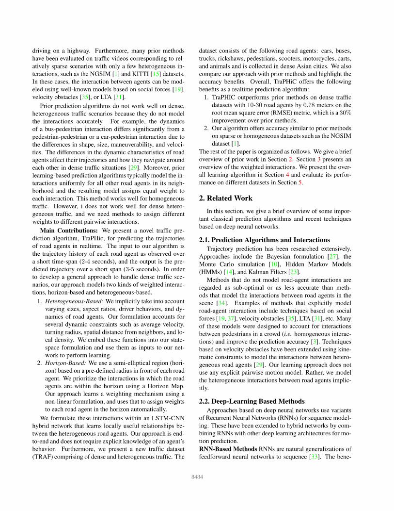
Figure 3. TraPHic Network Architecture: The ego agent is marked by the red dot. The green elliptical region around it is its neighborhood

and the cyan semi-elliptical region in front of it is its horizon. We generate input embeddings for all agents based on trajectory information

and heterogeneous dynamic constraints such as agent shape, velocity, and traffic concentration at the agent’s spatial coordinates, and other

parameters. These embeddings are passed through LSTMs and eventually used to construct the horizon map, the neighbor map and the ego

agent’s own tensor map. The horizon and neighbor maps are passed through separate ConvNets and then concatenated together with the

ego agent tensor to produce latent representations. Finally, these latent representations are passed through an LSTM to generate a trajectory

prediction for the ego agent.

Finally, the bottom-most layer corresponds to the ego

agent ai. Its input embedding, ei, passes sequentially

through a fully connected with ELU non-linearities [9], and

a single-layered LSTM to compute its hidden vector, hi.

The feature vectors from the horizon and neighbor layers,

fhz and fnb, are concatenated with hi to generate a final vec-

tor encoding

z := concat(hi, fhz, fnb) (4)

Finally, the concatenated encoding z passes through an

LSTM to compute the prediction for the next τ seconds.

4.1. Weighted Interactions

Our model is trained to learn weighted interactions in

both the horizon and neighborhood layers. Specifically, it

learns to assign appropriate weights to various pairwise in-

teractions based on the shape, dynamic constraints and be-

haviors of the involved agents. The horizon-based weighted

interactions takes into account the agents in the horizon of

the ego agent, and learns the “horizon map” Hi, given as

Hi = hjw|aj ∈ Hi (5)

Similarly, the neighbor or heterogeneous-based weighted

interactions accounts for all the agents in the neighborhood

of the ego agent, and learns the “neighbor map” Ni, given

as

Ni = hj |aj ∈ Ni (6)

During training, back-propagation optimizes the weights

corresponding to these maps by minimizing the loss be-

tween predicted output and ground truth labels. Our formu-

lation results in higher weights for prioritized interactions

(larger tensors in Horizon Map or blue vehicles in Figure 2)

and lower weights for less relevant interactions (smaller ten-

sors in Neighbor Map or green vehicles in Figure 2).

4.2. Implicit Constraints

Turning Radius: In addition to constraints such as posi-

tion, velocity and shape, constraints such as the turning ra-

dius of a road agent also affects its maneuverability, espe-

cially as it interacts with other road agents within some dis-

tance. For example, a car (a non-holonomic agent) cannot

alter its orientation in a short time frame to avoid collisions,

whereas a bicycle or a pedestrian can.

However, the turning radius of a road agent can be deter-

mined by the dimensions of the road agent, i.e., its length

and width. Since we include these parameters into our state-

space representation, we implicitly take into consideration

each agent’s turning radius constraints as well.

Driver Behavior: As stated in [7], velocity and acceler-

ation (both relative and average ) are clear indicators of

driver aggressiveness. For instance, a road agent with a

relative velocity (and/or acceleration) much higher than the

average velocity (and/or acceleration) of all road agents in

a given traffic scenario would be deemed as aggressive.

Moreover, given the traffic concentrations at two consecu-

tive spatial coordinates, c(x, y) and c(x+δx, y+δy), where

c(x, y) >> c(x + δx, y + δy), aggressive drivers move in

a “greedy” fashion in an attempt to occupy the empty spots

in the subsequent spatial locations. For each road agent, we

compute its concentration with respect to its neighborhood

and add this value to its input state-space.

Finally, the relative distance of a road agent from its

neighbors is another factor pertaining to how conservative

or aggressive a driver is. More conservative drivers tend to

8487

Dataset Method

RNN-ED S-LSTM S-GAN CS-LSTM TraPHic

NGSIM 6.86/10.02 5.73/9.58 5.16/9.42 7.25/10.05 5.63/9.91

Beijing 2.24/8.25 6.70/8.08 4.02/7.30 2.44/8.63 2.16/6.99

Table 1. Evaluation on sparse or homogeneous traffic datasets:

The first number is the average RMSE error (ADE) and the second

number is final RMSE error (FDE) after 5 seconds (in meters).

NGSIM is a standard sparse traffic dataset with few heterogeneous

interactions. The Beijing dataset is dense but with relatively low

heterogeneity. Lower value is better and bold value represents the

most accurate result.

maintain a healthy distance while aggressive drivers tend to

tail-gate. Hence, we compute the spatial distance of each

road agent in the neighborhood and encode this in its state-

space representation.

4.3. Overall Trajectory Prediction

Our algorithm follows a well-known scheme for predic-

tion [2]. We assume that the position of the road agent in the

next frame follows a bi-variate Gaussian distribution with

parameters µti, σ

ti = [(µx, µy)

ti, ((σx, σy)

ti)], and correla-

tion coefficient ρti. The spatial coordinates (xti, y

ti) are thus

drawn from N (µti, σ

ti , ρ

ti). We train the model by minimiz-

ing the negative log-likelihood loss function for the ith road

agent trajectory,

Li = −Στt+1 log(P((xt

i, yti)|(µ

ti, σ

ti , ρ

ti))). (7)

We jointly back-propagate through all three layers of our

network, optimizing the weights for the linear blocks, Con-

vNets, LSTMs, and Horizon and Neighbor Maps. The op-

timized parameters learned for the Linear-ELU block in the

horizon layer indicates the priority for the interaction in the

horizon of an road agent ai.

5. Experimental Evaluation

We describe our new dataset in Section 5.1. In Sec-

tion 5.2, we list all implementation details used in our train-

ing process. Next, we list the evaluation metrics and meth-

ods that we compare with, in Section 5.3. Finally, we

present the evaluation results in Section 5.4.

5.1. TRAF Dataset: Dense & Heterogeneous UrbanTraffic

We present a new dataset, currently comprising of 50videos of dense and heterogeneous traffic. The dataset

consists of the following road agent categories: car, bus,

truck, rickshaw, pedestrian, scooter, motorcycle, and other

road agents such as carts and animals. Overall, the dataset

contains approximately 13 motorized vehicles, 5 pedes-

trians and 2 bicycles per frame. Annotations were per-

formed following a strict protocol and each annotated

video file consists of spatial coordinates, an agent ID, and

an agent type. The dataset is categorized according to

camera viewpoint (front-facing/top-view), motion (mov-

ing/static), time of day (day/evening/night), and difficulty

level (sparse/moderate/heavy/challenge). All the videos

have a resolution of 1280 × 720. We present a compar-

ison of our dataset with standard traffic datasets in Table

3. The dataset is available at https://go.umd.edu/

TRAF-Dataset.

5.2. Implementation Details

We use single-layer LSTMs as our encoders and de-

coders with hidden state dimensions of 64 and 128, respec-

tively. Each ConvNet is implemented using two convolu-

tional operations each followed by an ELU non-linearity [9]

and then max-pooling. We train the network for 16 epochs

using the Adam optimizer [24] with a batch size of 128 and

learning rate of 0.001. We use a radius of 2 meters to define

the neighborhood and a minor axis length of 1.5 meters to

define the horizon, respectively. Our approach uses 3 sec-

onds of history and predicts spatial coordinates of the road

agent for up to 5 seconds (4 seconds for KITTI dataset). We

do not down-sample on the NGSIM dataset due to its spar-

sity. However, we use a down-sampling factor of 2 on the

Beijing and TRAF datasets due to their high density. Our

network is implemented in Pytorch using a single TiTan Xp

GPU. Our network does not use batch norm or dropout as

they can decrease accuracy. We include the experimental

details involving batch norm and dropout in the appendix

due to space limitations.

5.3. Evaluation Metrics and Comparison Methods

We use the following commonly used metrics [2, 18, 12]

to measure the performances of the algorithms used for pre-

dicting the trajectories of the road agents.

1. Average displacement error (ADE): The root mean

square error (RMSE) of all the predicted positions and

real positions during the prediction time.

2. Final displacement error (FDE): The RMSE distance

between the final predicted positions at the end of the

predicted trajectory and the corresponding true loca-

tion.

We compare our approach with the following methods.

• RNN-ED (Seq2Seq): An RNN encoder-decoder

model, which is widely used in motion and trajectory

prediction for vehicles [6].

• Social-LSTM (S-LSTM): An LSTM-based network

with social pooling of hidden states to predict pedes-

trian trajectories in crowds [2].

• Social-GAN (S-GAN): An LSTM-GAN hybrid

network to predict trajectories for large human

crowds [18].

• Convolutional-Social-LSTM (CS-LSTM): A variant

of S-LSTM adding convolutions to the network in [2]

in order to predict trajectories in sparse highway traf-

8488

Methods Evaluated on TRAF

RNN-ED S-LSTM S-GAN CS-LSTM TraPHic

Original Learned Original Learned Original Learned B He Ho Combined

3.24/5.16 6.43/6.84 3.01/4.89 2.89/4.56 2.76/4.79 2.34/8.01 1.15/3.35 2.73/7.21 2.33/5.75 1.22/3.01 0.78/2.44

Table 2. Evaluation on our new, highly dense and heterogeneous TRAF dataset. The first number is the average RMSE error (ADE) and

the second number is final RMSE error (FDE) after 5 seconds (in meters). The original setting for a method indicates that it was tested with

default settings. The learned setting indicates that it was trained on our dataset for fair comparison. We present variations of our approach

with each weighted interaction and demonstrate the contribution of the method. Lower is better and bold is best result.

Dataset# Frames Agents Visibility Density #Diff

(×103) Ped Bicycle Car Bike Scooter Bus Truck Rick Total (Km) (×103) Agents

NGSIM 10.2 0 0 981.4 3.9 0 0 28.2 0 1013.5 0.548 1.85 3

Beijing 93 1.6 1.9 12.9 16.4 0.005 3.28 3

TRAF 12.4 4.9 1.5 3.6 1.43 5 0.15 0.2 3.1 19.88 0.005 3.97 8

Table 3. Comparison of our new TRAF dataset with various traffic datasets in terms of heterogeneity and density of traffic agents.

Heterogeneity is described in terms of the number of different agents that appear in the overall dataset. Density is the total number of

traffic agents per Km in the dataset. The value for each agent type under “Agents” corresponds to the average number of instances of that

agent per frame of the dataset. It is computed by taking all the instances of that agent and dividing by the total number of frames. Visibility

is a ballpark estimate of the length of road in meters that is visible from the camera. NGSIM data were collected using tower-mounted

cameras (bird’s eye view), whereas both Beijing and TRAF data presented here were collected with car-mounted cameras (frontal view).

fic [12].

We also perform ablation studies with the following four

versions of our approach.

• TraPHic-B: A base version of our approach without

using any weighted interactions.

• TraPHic-Ho: A version of our approach without using

Heterogeneous-Based Weighted interactions, i.e., we

do not take into account driver behavior and informa-

tion such as shape, relative velocity, and concentration.

• TraPHic-He: A version of our approach without using

Horizon-Based Weighted interactions. In this case, we

do not explicitly model the horizon, but account for

heterogeneous interactions.

• TraPHic: Our main algorithm using both

Heterogeneous-Based and Horizon-Based Weighted

interactions. We explicitly model the horizon and

implicitly account for dynamic constraints and driver

behavior.

5.4. Results on Traffic Datasets

In order to provide a comprehensive evaluation, we com-

pare our method with state-of-the-art methods on several

datasets. Table 1 shows the results on the standard NGSIM

dataset and an additional dataset containing heterogeneous

traffic of moderate density. We present results on our new

TRAF dataset in Table 2.

TraPHic outperforms all prior methods we compared

with on our TRAF dataset. For a fairer comparison, we

trained these methods on our dataset before testing them

on the dataset. However, the prior methods did not gener-

alize well to dense and heterogeneous traffic videos. One

possible explanation for this is that S-LSTM and S-GAN

were designed to predict trajectories of humans in top-

down crowd videos whereas the TRAF dataset consists

of front-view heterogeneous traffic videos with high den-

sity. CS-LSTM uses lane information in its model and

weight all agent interactions equally. Since the traffic in

our dataset does not include the concept of lane-driving, we

used the version of CS-LSTM that does not include lane

information for a fairer comparison. However, it still led

to a poor performance since CS-LSTM does not account

for heterogeneous-based interactions. On the other hand,

TraPHic considers both heterogeneous-based and horizon-

based interactions, and thus produces superior performance

on our dense and heterogeneous dataset.

We visualize the performance of the various trajectory

prediction methods on our TRAF dataset Figure 5. Com-

pared to the prior methods, TraPHic produces the least de-

Figure 4. RMSE Curve Plot: We compare the accuracy of four

variants of our algorithm with CS-LSTM and each other based

on RMSE values on the TRAF dataset. On the average, using

TraPHic-He reduces RMSE by 15% relative to TraPHic-B, and

using TraPHic-Ho reduces RMSE by 55% relative to TraPHic-

B. TraPHic, the combination of TraPhic-He and TraPhic-Ho, re-

duces RMSE by 36% relative to TraPHic-Ho, 66% relative to

TraPHic-He, and 71% relative to TraPHic-B. Relative to CS-

LSTM, TraPHic reduces RMSE by 30%.

8489

Figure 5. Trajectory Prediction Results: We highlight the performance of various trajectory prediction methods on our TRAF dataset

with different types of road-agents. We showcase six scenarios with different density, heterogeneity, camera position (fixed or moving),

time of the day, and weather conditions. We highlight the predicted trajectories (over 5 seconds) of some of the road-agents in each scenario

to avoid clutter. The ground truth (GT) trajectory is drawn as a solid green line, and our (TraPHic) prediction results are shown using a

solid red line. The prediction results of other methods (RNN-ED, S-LSTM, S-GAN, CS-LSTM) are drawn with different dashed lines.

TraPHic predictions are closest to GT in all the scenarios. We observe up to 30% improvement in accuracy over prior methods over this

dense, heterogeneous traffic.

viation from the ground truth trajectory in all the scenarios.

Due to the significantly high density and heterogeneity in

these videos, coupled with the unpredictable nature of the

involved agents, all the predictions deviate from the ground

truth in the long term (after 5 seconds).

We demonstrate that our approach is comparable to prior

methods on sparse datasets such as the NGSIM dataset.

We do not outperform the current sate-of-the-art in such

datasets, since our algorithm tries to account for heteroge-

neous agents and weighted interactions even when interac-

tions are sparse and mostly homogeneous. Nevertheless, we

are at par with the state-of-the-art performance. Lastly, we

note that our RMSE value on the NGSIM dataset is quite

high, which we attribute to the fact that we used a much

higher (2X) sampling rate for averaging than prior methods.

Finally, we perform an ablation study to highlight the

contribution of our weighted interaction formulation. We

compare the four versions of TraPHic as stated in Sec-

tion 5.3. We find that the Horizon-based formulation con-

tributes more significantly to higher accuracy. TraPHic-He

reduces ADE by 15% and FDE by 20% over TraPHic-B,

whereas TraPHic-Ho reduces ADE by 55% and FDE by

58% over TraPHic-B. Incorporating both formulations re-

sults in the highest accuracy, reducing the ADE by 71% and

the FDE by 66% over TraPHic-B.

6. Conclusion, Limitations, and Future Work

We presented a novel algorithm for predicting the trajec-

tories of road agents in dense and heterogeneous traffic. Our

approach is end-to-end, dealing with traffic videos without

assuming lane-based driving. Furthermore, we are able to

model the interactions between heterogeneous road agents

corresponding to cars, buses, pedestrians, two-wheelers,

three-wheelers, and animals. We use an LSTM-CNN hy-

brid network to model two kinds of weighted interactions

between road agents: horizon-based and heterogeneous-

based. We demonstrate the benefits of our model over

state-of-the-art trajectory prediction methods on standard

datasets and on a novel dense traffic dataset. We observe

up to 30% improvement in prediction accuracy.

Our work has some limitations. Our model design is

motivated by some of the characteristics observed in dense

heterogeneous traffic. As a result, we do not outperform

prior methods on sparse or homogeneous traffic videos, al-

though our prediction results are comparable to prior meth-

ods. In addition, modeling heterogeneous constraints re-

quires the knowledge of the shapes and sizes of different

road agents. This information could be tedious to collect.

In the future, we plan to design a system that eliminates the

need for ground truth trajectory data and can directly pre-

dict the trajectories from an input video. We also intend to

use TraPHic for autonomous navigation in dense traffic.

7. Acknowledgments

This research is supported in part by ARO grant

W911NF19-1- 0069, Alibaba Innovative Research (AIR)

program, and Intel.

8490

References

[1] U.S. Federal Highway Administration. U.s. highway 101 and

i-80 dataset. 2005. 2, 3

[2] Alexandre Alahi, Kratarth Goel, Vignesh Ramanathan,

Alexandre Robicquet, Li Fei-Fei, and Silvio Savarese. So-

cial lstm: Human trajectory prediction in crowded spaces.

In Proceedings of the IEEE Conference on Computer Vision

and Pattern Recognition, pages 961–971, 2016. 1, 3, 4, 6

[3] Aniket Bera, Sujeong Kim, Tanmay Randhavane, Srihari

Pratapa, and Dinesh Manocha. Glmp-realtime pedestrian

path prediction using global and local movement patterns. In

Robotics and Automation (ICRA), 2016 IEEE International

Conference on, pages 5528–5535. IEEE, 2016. 2

[4] Jean-Yves Bouguet. Complete camera calibration toolbox

for matlab. 4

[5] Gary Bradski and Adrian Kaehler. Learning OpenCV: Com-

puter vision with the OpenCV library. ” O’Reilly Media,

Inc.”, 2008. 4

[6] D. Britz, A. Goldie, T. Luong, and Q. Le. Massive Explo-

ration of Neural Machine Translation Architectures. ArXiv

e-prints, Mar. 2017. 6

[7] Ernest Cheung, Aniket Bera, Emily Kubin, Kurt Gray,

and Dinesh Manocha. Identifying driver behaviors using

trajectory features for vehicle navigation. arXiv preprint

arXiv:1803.00881, 2018. 3, 5

[8] Fang-Chieh Chou, Tsung-Han Lin, Henggang Cui, Vladan

Radosavljevic, Thi Nguyen, Tzu-Kuo Huang, Matthew

Niedoba, Jeff Schneider, and Nemanja Djuric. Predicting

motion of vulnerable road users using high-definition maps

and efficient convnets. 2018. 3

[9] Djork-Arne Clevert, Thomas Unterthiner, and Sepp Hochre-

iter. Fast and accurate deep network learning by exponential

linear units (elus). arXiv preprint arXiv:1511.07289, 2015.

4, 5, 6

[10] Simon Danielsson, Lars Petersson, and Andreas Eidehall.

Monte carlo based threat assessment: Analysis and improve-

ments. In Intelligent Vehicles Symposium, 2007 IEEE, pages

233–238. IEEE, 2007. 2

[11] Nachiket Deo, Akshay Rangesh, and Mohan M. Trivedi.

How would surround vehicles move? A unified framework

for maneuver classification and motion prediction. CoRR,

abs/1801.06523, 2018. 1

[12] Nachiket Deo and Mohan M Trivedi. Convolutional so-

cial pooling for vehicle trajectory prediction. arXiv preprint

arXiv:1805.06771, 2018. 1, 3, 4, 6, 7

[13] N. Djuric, V. Radosavljevic, H. Cui, T. Nguyen, F.-C. Chou,

T.-H. Lin, and J. Schneider. Short-term Motion Prediction of

Traffic Actors for Autonomous Driving using Deep Convo-

lutional Networks. ArXiv e-prints, Aug. 2018. 3

[14] Jonas Firl, Hagen Stubing, Sorin A Huss, and Christoph

Stiller. Predictive maneuver evaluation for enhancement of

car-to-x mobility data. In Intelligent Vehicles Symposium

(IV), 2012 IEEE, pages 558–564. IEEE, 2012. 2

[15] Andreas Geiger, Philip Lenz, Christoph Stiller, and Raquel

Urtasun. Vision meets robotics: The kitti dataset. Interna-

tional Journal of Robotics Research (IJRR), 2013. 2, 3

[16] Alex Graves. Generating sequences with recurrent neural

networks. arXiv preprint arXiv:1308.0850, 2013. 4

[17] Karol Gregor, Ivo Danihelka, Alex Graves, Danilo Jimenez

Rezende, and Daan Wierstra. Draw: A recurrent

neural network for image generation. arXiv preprint

arXiv:1502.04623, 2015. 3

[18] A. Gupta, J. Johnson, L. Fei-Fei, S. Savarese, and A. Alahi.

Social GAN: Socially Acceptable Trajectories with Genera-

tive Adversarial Networks. ArXiv e-prints, Mar. 2018. 1, 3,

4, 6

[19] Dirk Helbing and Peter Molnar. Social force model for

pedestrian dynamics. Physical review E, 51(5):4282, 1995.

2

[20] Xinyu Huang, Xinjing Cheng, Qichuan Geng, Binbin Cao,

Dingfu Zhou, Peng Wang, Yuanqing Lin, and Ruigang Yang.

The apolloscape dataset for autonomous driving. 3

[21] MLL Iannini and Ronald Dickman. Kinetic theory of ve-

hicular traffic. American Journal of Physics, 84(2):135–145,

2016. 4

[22] Phillip Isola, Jun-Yan Zhu, Tinghui Zhou, and Alexei A

Efros. Image-to-image translation with conditional adver-

sarial networks. 3

[23] Rudolph Emil Kalman. A new approach to linear filtering

and prediction problems. Transactions of the ASME–Journal

of Basic Engineering, 82(Series D):35–45, 1960. 2

[24] Diederik P Kingma and Jimmy Ba. Adam: A method for

stochastic optimization. arXiv preprint arXiv:1412.6980,

2014. 6

[25] Christian Ledig, Lucas Theis, Ferenc Huszar, Jose Caballero,

Andrew Cunningham, Alejandro Acosta, Andrew P Aitken,

Alykhan Tejani, Johannes Totz, Zehan Wang, et al. Photo-

realistic single image super-resolution using a generative ad-

versarial network. 3

[26] Namhoon Lee, Wongun Choi, Paul Vernaza, Christopher B

Choy, Philip HS Torr, and Manmohan Chandraker. Desire:

Distant future prediction in dynamic scenes with interacting

agents. In Proceedings of the IEEE Conference on Computer

Vision and Pattern Recognition, 2017. 1, 3

[27] Stephanie Lefevre, Christian Laugier, and Javier Ibanez-

Guzman. Exploiting map information for driver intention

estimation at road intersections. In Intelligent Vehicles Sym-

posium (IV), 2011 IEEE, pages 583–588. IEEE, 2011. 2

[28] Alon Lerner, Yiorgos Chrysanthou, and Dani Lischinski.

Crowds by example. In Computer Graphics Forum, vol-

ume 26, pages 655–664. Wiley Online Library, 2007. 3

[29] Y. Ma, D. Manocha, and W. Wang. AutoRVO: Local Nav-

igation with Dynamic Constraints in Dense Heterogeneous

Traffic. In Computer Science in Cars Symposium (CSCS).

ACM, 2018. 2

[30] Y. Ma, X. Zhu, S. Zhang, R. Yang, W. Wang, and D.

Manocha. TrafficPredict: Trajectory Prediction for Hetero-

geneous Traffic-Agents. ArXiv e-prints, Nov. 2018. 1, 3

[31] Stefano Pellegrini, Andreas Ess, Konrad Schindler, and Luc

Van Gool. You’ll never walk alone: Modeling social behav-

ior for multi-target tracking. In Computer Vision, 2009 IEEE

12th International Conference on, pages 261–268. IEEE,

2009. 2, 3

8491

[32] Matthias Schreier, Volker Willert, and Jurgen Adamy.

Bayesian, maneuver-based, long-term trajectory prediction

and criticality assessment for driver assistance systems. In

Intelligent Transportation Systems (ITSC), 2014 IEEE 17th

International Conference on, pages 334–341. IEEE, 2014. 1

[33] Ilya Sutskever, Oriol Vinyals, and Quoc V Le. Sequence to

sequence learning with neural networks. In Advances in neu-

ral information processing systems, pages 3104–3112, 2014.

2

[34] Peter Trautman and Andreas Krause. Unfreezing the robot:

Navigation in dense, interacting crowds. In Intelligent

Robots and Systems (IROS), 2010 IEEE/RSJ International

Conference on, pages 797–803. IEEE, 2010. 2

[35] Jur Van Den Berg, Stephen J Guy, Ming Lin, and Di-

nesh Manocha. Reciprocal n-body collision avoidance. In

Robotics research, pages 3–19. Springer, 2011. 2

[36] Anirudh Vemula, Katharina Muelling, and Jean Oh. Social

attention: Modeling attention in human crowds. In 2018

IEEE International Conference on Robotics and Automation

(ICRA), pages 1–7. IEEE, 2018. 1, 3

[37] Kota Yamaguchi, Alexander C Berg, Luis E Ortiz, and

Tamara L Berg. Who are you with and where are you go-

ing? In Computer Vision and Pattern Recognition (CVPR),

2011 IEEE Conference on, pages 1345–1352. IEEE, 2011. 2

[38] Zhong-Qiu Zhao, Peng Zheng, Shou-tao Xu, and Xindong

Wu. Object Detection with Deep Learning: A Review. arXiv

e-prints, page arXiv:1807.05511, Jul 2018. 3

8492