Travel Time Estimation in the Age of Big Data

Dimitris Bertsimas, Arthur Delarue, Patrick Jaillet, Sebastien MartinOperations Research Center, Massachusetts Institute of Technology

May 2018∗

Abstract

Twenty-first century urban planners have identified the under-standing of complex city traffic patterns as a major priority, leadingto a sharp increase in the amount and the diversity of traffic databeing collected. For instance, taxi companies in an increasing numberof major cities have started recording metadata for every individualcar ride, such as its origin, destination and travel time. In this pa-per, we show that we can leverage network optimization insights toextract accurate travel time estimations from such origin-destinationdata, using information from a large number of taxi trips to recon-struct the traffic patterns in an entire city. We develop a methodthat tractably exploits origin-destination data, which, because of itsoptimization framework, could also take advantage of other sourcesof traffic information. Using synthetic data, we establish the robust-ness of our algorithm to high variance data, and the interpretabilityof its results. We then use hundreds of thousands of taxi travel timesobservations in Manhattan to show that our algorithm can provideinsights about urban traffic patterns on different scales and accuratetravel time estimations throughout the network.

1 Introduction

In today’s increasingly dense urban landscapes, traffic congestion is an evermore prevalent issue. As flows of goods and people increase, billions of dollarsin potential savings are at stake, making the understanding of traffic patternsa major urban planning priority.

∗Accepted for publication in Operations Research

1

A main goal of traffic studies is travel time estimation, which in the broad-est sense consists of evaluating the time necessary to travel from any originO to any destination D. This goal is difficult to achieve because travel timesdepend on a range of effects at different timescales, from the structure of thenetwork (number of lanes on each road, speed limit, etc.) over the long term,to the state of congestion of the network over the medium term, to a host ofsmall random events (missed lights, etc.) over the very short term. Becauseof the sheer number and diversity of these sources of uncertainty, most gen-eral approaches to travel time estimation consist of finding parameters thatdescribe a distribution or set of distributions from which the travel time fromO to D is sampled.

Travel time estimation is often combined with the related goal of routing,especially in the short to medium-term planning case. In this case, the goalis to evaluate the time necessary to travel from O to D and find at least onepath that drivers could use to achieve this estimate, relating the travel timeestimate to interpretable network properties. In this paper, we present anovel method to estimate typical travel times for each road in a city networkusing taxi data, thus providing reasonable paths and total trip time estimatesfor any origin and destination in the network.

1.1 The Need for a Generalized Approach to TravelTime Estimation

The problem of inferring traffic patterns from diverse measurements is afundamental step behind the resolution of many complex questions in trans-portation and logistics. A simple cost function on the individual arcs of thenetwork can often form a building block of a more complex network study,such as recent work by Pioro et al. (2016) presenting a novel understand-ing of resilient networks. Furthermore, many network problems specificallyrequire a travel time estimate for each arc: for instance, Nikolova and Stier-Moses (2014), who develop a new model for traffic assignment that takesinto account network uncertainty, present an approach starting from a priorestimate of the expected travel times of individual arcs in the network. Evenin examples such as the aforementioned work or that of Jaillet et al. (2016),both of which generally consider travel time to be a stochastic quantity, agood estimate for the network travel times is a valuable asset in order todefine a prior or an uncertainty set for this uncertain quantity, laying thegroundwork to answer more complex questions about the network.

In a real-world setting, there are different ways to obtain traffic data ina network, each leading to different travel time estimation methods. A pop-

2

ular approach uses fixed detectors that provide information about traffic atparticular points in the network, most commonly loop sensors as in Coifman(2002), or more advanced methods as in Li and Rose (2011) that exploitcommunication between sensors to identify the same vehicle at different lo-cations. Another popular approach, as in Jenelius and Koutsopoulos (2013),uses so-called “floating-car” data, where GPS-equipped vehicles record theirlocation and speed at fixed time intervals, which can range from a few sec-onds to a few minutes. The path followed by the vehicle between “pings”of the GPS device can be inferred in a variety of ways, from probabilisticmodels in Hofleitner et al. (2012) to tensor decomposition in Wang et al.(2014).

A third area of study involves easily gatherable “origin-destination” (OD)data, that only records the time and location at the beginning and at theend of a trip, as, for example, collected by taxis or cellphone towers. Log-ging this data instead of high-density floating-car data increases the privacyof the taxi driver and passenger because the details of the followed routeare not recorded. It also treats the network as a black box, only makingmeasurements when the user enters and exits. OD data can be gatheredfor different purposes, and the methods we develop here in the context ofvehicle traffic can be extended to other types of networks, including rail-ways, subways, and bicycle and pedestrian networks (see recent studies suchas Hanseler et al. (2017)), or combinations of such networks. Nevertheless,this generality makes the travel time estimation harder: the problem of si-multaneously determining paths and travel times based on origin-destinationdata only is close to the Inverse Shortest Path Length Problem (ISPL), anNP-hard problem which has also received some attention by Hung (2003).

In recent years, the New York City Taxi and Limousine Commission(NYCTLC (2016)) has maintained a complete public record of yellow cabrides within the city. The database contains relevant metadata such as theorigin, destination, fare, distance and time traveled for over 170 million ridesper year, and has been exploited for a variety of purposes, as shown in Yang(2015). Despite the data’s size and availability, however, it has not beenused very much for travel time estimation. Wang et al. (2015) develop amachine learning method based on k-nearest neighbors matching, while Santiet al. (2014) describe a very simple smoothing heuristic. Meanwhile, Zhanet al. (2013)’s more model-oriented approach develops a full probabilisticpath selection scheme.

3

1.2 Our Contributions

The main contribution of this paper is a tractable methodology to solve thetravel time estimation and routing problem in a real-world setting on a largenetwork, which has a number of desirable properties.

First, we use very few assumptions about the data: to provide travel timeestimates, we only ask for a set of trips within a known network for whichan origin, a destination and a travel time are recorded. In particular, wedo not require information about the demand structure in the network. Wedesign a simple static model of traffic based on shortest path theory. Thissimplicity allows us to develop a multipurpose network optimization methodthat can leverage large amounts of high-variance origin-destination data tobuild an estimate of city travel times that is accurate both in and out ofsample. Moreover, this method is general enough to be able to handle othersources of data, including floating cars and loop sensors.

Furthermore, the method also recovers interpretable city traffic and rout-ing information from this potentially noisy and incomplete data. We estimatea single parameter for each edge, which enhances the interpretability of theresults (see Figure 1 for an example). In order to avoid overfitting, partic-ularly in regions of the city where little data is available, we add a simpleregularization term to the model. The method provides insight on trafficpatterns at the scale of a few city blocks, as well as at the scale of the entirenetwork, and also allows us to quickly find viable paths associated with ourtravel time estimates.

Solving this estimation problem to optimality at an impactful scale isgenerally intractable. For this reason, we develop a novel iterative algorithmthat provides good solutions, by solving a sequence of large second-ordercone problems (SOCPs), which modern solvers can tractably handle. Weverify the accuracy of this algorithm in a variety of settings and show thatit provides high-quality solutions. The method is tractable, determining thetypical paths and travel times in the 4300-node Manhattan network over athree-hour time window in under 20 minutes.

In Section 2, we formulate an optimization problem that gives both ac-curate origin-destination travel time estimates and interpretable link traveltimes and routing paths. In Section 3, we introduce an iterative algorithmthat can compute solutions to this optimization in large scale settings. InSection 4, using synthetic data we show that the solutions of this algorithmare near-optimal and that the simplifications we made for tractability didnot impact accuracy and interpretability. In Section 5, we show that thisalso extends to real-world situations and we present results on Manhattantaxi data.

4

Figure 1: Close-up of Manhattan with the arc travel times estimated byour method between 9 and 11 AM. The color of each arc represents thespeed along that arc as a percentage of the reference velocity v0 = 13.85kph (average velocity in Manhattan on weekdays). We can identify trafficeffects at the scale of the city (Midtown congestion) and at the scale of asingle street (the ramp onto the highway on the eastern shore of Manhattanis congested).

2 Methodology

In this section, we define the probabilistic setting of travel time estimation,and introduce a simple traffic model that leverages the knowledge of therouting network to represent travel time estimates in the lower dimensionalspace of network arc travel times. This allows us to create an optimizationformulation that uses origin-destination data to build an interpretable imageof the network travel times, and at the same time provide accurate traveltime estimates.

2.1 Problem Statement: Estimating Travel Times FromData

Data. We consider a road network, represented as a directed graph G =(V,E). On this graph, we are given a data set of origin-destination traveltime values in the network, of the form (o, d, T ) with (o, d) ∈ V × V theorigin and destination nodes and T ∈ R+ the corresponding observed traveltime. Data corresponding to this general description can be obtained inmany different ways. For example, the set of observed travel times for taxi

5

trips that started between 12pm and 1pm on 2016 Wednesdays in Manhattanwould be a valid example of such a data set, as would the set of stop-to-stoptravel times for Boston school buses in the academic year 2016-17.

Some origin-destination pairs have several travel time observations in thedata set, while others have none. We can therefore define W ⊂ V ×V as thesubset of origin-destination pairs for which we have data: for each (o, d) ∈ Wwe are given travel times {T i

od}nodi=1, realized on nod distinct trips from o to d.

Probabilistic Setting. We would like to estimate the times of trips thatare “similar” to the trips that are given in the data set, but may not havebeen observed in the data. In other words, given any origin-destination pair(o, d) ∈ V 2, we would like to provide a point estimate Tod of the time it takesto go from o to d. To properly define these estimates for all origin-destinationpairs, we describe a simple probabilistic setting.

Each observation of the data-set is assumed to be independently sam-pled from the same probability distribution. This sampling process goes asfollows: the origin and destination nodes (o, d) are sampled from a discretedistribution D in V 2. Then, conditioned on having an origin o and a des-tination d, the observed travel times {T i

od}nodi=1 are assumed to be sampled

independently from the distribution Dod. Note that Dod can be different foreach (o, d). We assume that our data set was built by following this samplingprocess, but that we do not know the distributions D or Dod. We will holdthese probabilistic assumptions to be true throughout this paper, includingour experiments on synthetic data in Section 4. In Section 5, we will showthat our results extend to real-world data that does not necessarily verifyour probabilistic assumptions.

We want to obtain a point estimate Tod of the distribution Dod for everypair (o, d) ∈ V×V . Specifically, we would like to estimate the geometric meanof the distribution Dod : exp(ETod∼Dod

[log(Tod)]). We choose the geometricmean instead of the standard mean because we think that the quality of traveltime estimations is perceived on a multiplicative rather than an additive scale,as we discuss in the next paragraph.

To understand the choice of estimating the geometric mean, note thatthe geometric means of all the distributions Dod are estimates that minimize

6

the overall mean squared log error (MSLE) :

MSLE((Tod)(o,d)∈V 2) = E(o,d)∼D,Tod∼Dod

[(log(Tod)− log(Tod)

)2](1)

= E(o,d)∼D,Tod∼Dod

[(log(Tod)− ETod∼Dod

[log(Tod)])2]

(2)

+ E(o,d)∼D

[(log(Tod)− ETod∼Dod

[log(Tod)])2]

. (3)

Note that the expectations are taken with respect to the distributionsD and Dod. The MSLE decomposes into the mean log variance of the data(2) which is independent of our estimates, and the mean squared log bias(MSLB) (3) which is a measure of the distance of each estimate Tod fromthe geometric mean of Dod. Using the MSLE implies that an estimate thatis twice an observed value is equally bad as an estimate that is half of it.Additionally, a 30-second estimation error is a lot worse for a trip that last2 minutes than for a trip that lasts 15 minutes. This is what we want andwhy we chose the log scale and geometric mean estimates.

Model. In practice, we do not observe all the possible (o, d) pairs, whichmakes it hard to estimate the geometric mean of Dod using only the data thathas origin o and destination d. Nonetheless, the estimates of the distributionsDod are typically related: for example, a trip from o to d and a trip from o′ to dwhere o and o′ are geographically close will have similar travel time estimates.Therefore, we leverage the network structure by introducing parameters tijthat represent the typical travel time along any arc (i, j) ∈ E, and use themto compute our estimates Tod.

We define a path Pod from o to d as a series of consecutive arcs (withoutcycles), starting at o and ending at d, and Pod to be the finite set of allpossible paths from o to d. For each possible path Pod ∈ Pod, we modelthe point estimate of the total travel time along this path to be TPod

=∑(i,j)∈Pod

tij. Because our data set provides no information as to which pathwas followed to realize a given travel time, we assume that drivers use thefastest paths available. We thus select Pod = argminPod∈Pod

∑(i,j)∈Pod

tij, and

define our point estimate to be Tod = TPod=∑

(i,j)∈Podtij. As a consequence,

given the parameters tij, our model chooses the point estimates Tod(t) =minPod∈Pod

∑(i,j)∈Pod

tij, where t is simply shorthand for the vector (tij)(i,j)∈E(following standard boldfaced vector notation).

To use this model, we must only provide |E| parameters, which is gen-erally much less than the |V |2 estimates we want to obtain. The model is

7

also interpretable, as we expect the values tij to be representative of thetypical travel-times along arc (i, j) ∈ E. We acknowledge that the shortest-path assumption itself can be questioned. From a behavioral standpoint,taxi drivers may have other objectives in mind, such as maximizing revenueor minimizing fuel consumption; in addition, Dial (1971) showed that short-est paths can be sensitive to changes in travel time. However, we find thatdespite this modeling assumption, our results on real data are interpretableand reasonably accurate.

Parameter Estimation. We want to use the observed travel times T iod to

estimate the model parameters tij. Following our goal to have estimates asclose as possible to the geometric mean ofDod, we want to find the values of tijthat minimize the MSLE of the estimates Tod. Because the distributions Dod

and D are unknown, we approximate them with the empirical distributionof our observations and we obtain the following minimization problem:

mint

∑(o,d)∈W

nod∑i=1

(log Tod(t)− log T iod)

2, (4)

which is equivalent to

mint

∑(o,d)∈W

nod(log Tod(t)− log Tod)2, (5)

where Tod = (∏nod

i=1 Tiod)

1/nod , the geometric mean of all the observed traveltimes from o to d.

Regularization. In order to generalize well out of sample, we need to adda regularization term to the empirical MSLE. This is important because wemay not have sampled enough data from D and Dod, and the empirical MSLE(4) may not be a good approximation of the MSLE (1). Leveraging ourknowledge of the city network, we hypothesize that two similar intersectingor consecutive roads should have similar traffic speeds by default. Two arcs(i, j) and (k, l) are called neighboring when they represent consecutive orintersecting roads with the same “type”. These types are defined through ourknowledge of the routing network, and differentiate highways, major arteriesand smaller roads. The neighboring relationship is written as (i, j)↔ (k, l).This regularization is somewhat unusual in traffic studies, but it is effective inpractice and will only influence our estimation when we do not have enoughdata. Adding the regularization term to our objective yields:∑

(o,d)∈W

nod

(log Tod − log Tod

)2+ λ

∑(i,j)↔(k,l)

∣∣∣∣ tijdij − tkldkl

∣∣∣∣ 2

dij + dkl, (6)

8

where dij corresponds to the length in meters of the arc (i, j) in the routingnetwork,

∑(i,j)↔(k,l) represent the sum over all pairs of neighboring arcs (i, j)

and (k, l) and the parameter λ represents the strength of the regularization.In other words, we minimize the difference in speed of neighboring roads, withthe weighting factor 2/(dij+dkl) ensuring that continuity is more important inshorter neighboring roads (where constant velocity is a better approximation)than in longer ones.

2.2 MIO Formulation

We can now estimate the parameters tij from the data by solving the followingmixed-integer formulation with linear constraints and a non-linear objective:

minT, t,z

∑(o,d)∈W

nod

(log Tod − log Tod

)2+ λ

∑(i,j)↔(k,l)

∣∣∣∣ tijdij − tkldkl

∣∣∣∣ 2

dij + dkl

(7a)

s.t. Tod ≤∑

(i,j)∈P `od

tij ∀(o, d) ∈ W, P `od ∈ Kod (7b)

Tod ≥∑

(i,j)∈P `od

tij −M(1− z`od) ∀(o, d) ∈ W, P `od ∈ Kod (7c)

∑`

z`od = 1 ∀(o, d) ∈ W (7d)

z`od ∈ {0, 1} ∀(o, d) ∈ W, ` ∈ {1, . . . , |Kod|}(7e)

tij ≥ aij ∀(i, j) ∈ E. (7f)

The objective (7a) is the parameter estimation cost introduced in (6). Foreach (o, d) ∈ W , the constraints enforce that Tod = minPod∈Kod

∑(i,j)∈Pod

tij,

i.e. Tod is the time of the shortest path from o to d out of all the paths in Kod.This non-linear shortest path constraint is enforced using the binary variableszlod that represent which path P `

od ∈ Kod is the shortest path, together withthe constraints (7b), (7d) and the big-M constraints (7c). Typically, Kod =Pod is the set of all paths from o to d, but the formulation generalizes to anyother subset Kod ⊂ Pod. Finally, the constraints (7f) introduce the boundsaij to enforce a speed limit on the arc travel times tij.

9

2.3 Iterative Path Generation

For each (o, d) ∈ W , formulation (7) requires one binary variable for eachpath going from o to d. The number of paths is typically exponential in thesize of the graph, so we need to reduce the number of paths to consider if wewant to be able to solve (7). It turns out the formulation is naturally suitedfor an iterative approach. Assume we start with a small set of paths P0

od forevery origin-destination pair in the dataset. We can solve the problem in (7)by considering the set of paths Kod = P0

od instead of the much larger Kod =Pod. This yields values of tij, for which we can recompute new shortest pathsin the network using any shortest-path algorithm. If for a given (o, d), the newshortest path has length less than Tod, then we know that the minimum pathlength computed over P0

od is not equal to the minimum path length over Pod.In this case, we add the new shortest path P 1

od to our set of paths, obtainingthe set P1

od = P0od∪{P 1

od}. We can then re-solve (7) using P1od instead of P0

od,and iterate this process. If instead the new shortest path for each (o, d) haslength equal to Tod, then we know we have already found reasonable paths,reaching a stopping point for the algorithm. The algorithm thus generatesan increasing list of path candidates Pk

od for each iteration k and (o, d) ∈ W ,so that the shortest paths P k

od are added to the path candidates of the nextiteration, e.g. Pk+1

od = Pkod ∪ {P k

od}.This iterative approach is inspired by cutting plane algorithms in linear

optimization. In practice, most paths between o and d are not remotely closeto being the shortest and would never even be considered by drivers lookingto travel from o to d. Although this iterative method does not necessarily con-verge to the global optimum of (7) with Kod = Pod, we will show empiricallythat it yields good results for large problems, does not exhibit pathologicallocal optima when used with appropriate regularization and typically con-verges in a few steps. Additionally the algorithm is always interpretable: thesolution at any iteration k corresponds to the optimal solution of the problemif the drivers only consider the paths in Pk

od.

3 Solving Large-Scale Problems

Even with the iterative path generation presented in 2.3, the optimizationproblem (7) cannot be tractably solved for most problems of interest. Themain reasons are that the objective is non-convex, and that there are atleast O(|W |) binary variables, which makes it impossible for state-of-the-artsolvers to give interesting solutions in a reasonable time for problems withmore than 1000 data-points and routing networks that represent real cities.

10

Actually, solving this problem to optimality relates to the problem of pathreconstruction in a graph (sometimes called the Inverse Shortest Path Lengthproblem), an NP-hard problem, as discussed in Hung (2003). We presenta tractable approach that produces good solutions, allowing us to handlehundreds of thousands of data points in networks with tens of thousands ofarcs.

3.1 Adapting the shortest path constraint

In order to handle a large number of data points, we need to discard thebinary variables z`od introduced in (7e). One way to do this is to modifythe constraint Tod = minPod∈Kod

∑(i,j)∈Pod

tij. An interesting solution can bebuilt by fixing the values of the binary variable, i.e., choosing which pathshould be the shortest for each (o, d) ∈ W . Indeed, if the shortest path inKod is chosen to be P ∗od, then the shortest path constraints (7b)-(7e) triviallybecome:

Tod =∑

(i,j)∈P ∗od

tij ∀(o, d) ∈ W, (8a)

Tod ≥∑

(i,j)∈Pod

tij ∀(o, d) ∈ W, Pod ∈ Kod. (8b)

For this formulation to become useful, we need a clever way to choose P ∗odfor each (o, d) ∈ W . Our iterative path generation algorithm introducedin Section 2.3 provides a good candidate. At iteration k, the algorithmcomputes the shortest path P k

od for each (o, d) ∈ W . This path can beviewed as our “best estimate” of the true path at iteration k, and is one ofthe paths we consider at iteration k + 1. For this reason, we choose to usethis path as the chosen shortest path for the next iteration k + 1, settingP ∗od = P k

od.In the end, the results on synthetic data in Section 4 and on real data

in Section 5 show that this method, appropriately regularized, yields inter-pretable high-quality solutions and empirically converges. Our intuition isthe following: this path estimation may not seem perfect, but the tractabil-ity gains allow us to use orders of magnitude more data, which will improvethe accuracy of the tij parameters and the Tod estimates, thus allowing us tocompute better paths at each iteration.

3.2 Towards a Convex Objective

The left term in the minimization objective (7a) is nonconvex and not easilyoptimized by traditional optimization solvers. We want to find a surrogate

11

that is convex, tractable, and a good approximation of the original squaredlog cost. More specifically, we want to find a convex loss function ` such that`(Tod, Tod) = (log(Tod)− log(Tod))

2 + o((Tod − Tod)2), and such that ` is alsounbiased in the multiplicative space, i.e. `(aTod, Tod) = `(Tod

a, Tod) for any

scalar a > 0.

A good candidate is the maximum ratio loss: `(Tod, Tod) =(

max(

Tod

Tod, Tod

Tod

)− 1)2

.

It is a convex function of the variable Tod that has all the desired properties.Our objective thus becomes:

∑(o,d)∈W

nod

(max

(Tod

Tod,TodTod

)− 1

)2

+ λ∑

(i,j)↔(k,l)

∣∣∣∣ tijdij − tkldkl

∣∣∣∣ 2

dij + dkl(9)

We want to be able to solve the corresponding optimization with hundredsof thousands of data-points. To the best of our knowledge, only state-of-the-art LP and SOCP solvers are able to handle formulations with hundreds ofthousands of variables and constraints. As a consequence, we would like toslightly modify our formulation to be able to formulate it as an SOCP. Allwe need to do is replace the squared losses by absolute values, yielding themodified objective:

∑(o,d)∈W

nod max

(Tod

Tod,TodTod

)+ λ

∑(i,j)↔(k,l)

∣∣∣∣ tijdij − tkldkl

∣∣∣∣ 2

dij + dkl(10)

This new objective allows us to reformulate each iteration as an SOCP:

minT, t,x

∑(o,d)∈W

nodxod + λ∑

(i,j)↔(k,l)

∣∣∣∣ tijdij − tkldkl

∣∣∣∣ 2

dij + dkl(11a)

s.t. Tod =∑

(i,j)∈P ∗od

tij ∀(o, d) ∈ W, (11b)

Tod ≥∑

(i,j)∈Pod

tij ∀(o, d) ∈ W, Pod ∈ Kod,

(11c)

xod ≥TodTod

∀(o, d) ∈ W, (11d)

xod ≥Tod

Tod∀(o, d) ∈ W, (11e)

tij ≥ aij ∀(i, j) ∈ E. (11f)

12

where xod = max(

Tod

Tod, Tod

Tod

). The objective can be formulated as linear, and

all the constraints are linear except (11e), which can be reformulated as thefollowing second-order cone constraint:(

xod + Tod

)≥∥∥∥∥(Tod − xod2

√Tod

)∥∥∥∥ . (12)

Replacing the squared losses by absolute values makes our new formulationmore robust to outliers and more tractable, but weakens the case for replacingthe observations T i

od that share the same (o, d) with their geometric mean Tod.Once more, we trade some modeling rigor for the ability to use more data,and we will show that this choice is empirically justified.

3.3 A Tractable Algorithm

We now summarize our tractable algorithm for large-scale static travel timeestimation.

1. Choose a regularization parameter λ and an initial set of arc travel-times: (t0ij)(i,j)∈E. We will show in the next sections that our resultsare not sensitive to these choices. For each (o, d) ∈ K, start with anempty set of paths Pod = ∅. Then start Step 2 with iteration k = 1.

2. For each iteration k, do the following:

3. Use an efficient, parallelized shortest-path algorithm to compute all theshortest paths (P k

od)(o,d)∈W , using the arc travel-times (tk−1ij )(i,j)∈E. Add

these paths to the previous set of paths Pkod = Pk−1

od ∪{P kod}. If there is a

limit Π on the number of paths we can store (for memory or tractabilityreasons), remove the path of Pk

od with the longest travel-time to makesure that |Pk

od| ≤ Π.

4. Solve the optimization problem (11), using the newly computed short-est paths P ∗od = P k

od, to obtain the new arc travel-times (tkij)(i,j)∈E.

5. If a convergence criterion is met, stop the algorithm and return thetimes (tkij)(i,j)∈E. Else, start iteration k + 1 and go to Step 2.

In the end, our algorithm returns a set of arc travel-times, that can be usedto compute shortest paths and travel time estimations Tod for any origin-destination pair in the network. We propose a convergence criterion basedon path differences.

13

Definition 1 (Path difference). Given a node pair (o, d) and two paths PAod

and PBod, the path difference d(PA

od, PBod) is defined as the average of the number

of arcs in PAod that are not in PB

od and the number of arcs in PBod that are not

in PAod.

At each iteration k, we can compute the path difference between the newpath P k

od and the path of the previous iteration P k−1od for each (o, d) ∈ W .

We stop our algorithm when the mean path difference across all (o, d) ∈ Wis less than a threshold δ, i.e. 1

|W |∑

(o,d)∈W d(P kod, P

k−1od ) < δ. In this paper,

we fix δ to a small value: δ = 0.5. We chose this value because we noticedthat our estimates Tod were not improving in subsequent iterations, for thespecific applications of this paper. In this situation, the algorithm tends toconverge in less than 10 iterations.

3.4 A General Model

The ability to solve the travel time estimation and routing problem usingonly origin-destination data is useful because it makes minimal assumptionson the format of the data. However, in some cases more data is available, forinstance from loop sensors or floating car probes (see Section 1.1). Due toits optimization-based framework, our method is flexible enough to handlemany additional forms of data.

The method presented in the previous section is designed under the as-sumption that for every (o, d) in the set of input node pairs W ⊂ V × V ,we are only given a finite number of sample travel times, from which wecompute a geometric mean Tod, with no information about the path takenby the drivers. Constraint (11b) reflects the algorithm’s attempt to guessthe correct path, assuming that the drivers are trying to minimize drivingtimes. If we assume now that for some (o, d) ∈ W , we are given not only atravel time T obs

od , but also the used path P obsod , then we can add a term in the

objective penalizing the distance between the observation T obsod and the sum∑

(i,j)∈P obsodtij of link travel times along the path P obs

od .

Another form of traffic data that is commonly available comes from loopsensors/traffic cameras, which can sometimes measure traffic velocity on agiven set of arcs L ⊆ E. For example, Wang and Nihan (2000) shows thata single loop detector on a highway is enough to provide accurate speedestimates. A velocity measurement on arc (i, j) is easily integrated into ourmodel, by adding a term in the objective that penalizes the distance of tijfrom its measurement.

Thus, though our method is designed with minimal data in mind, it caneasily incorporate additional information about the network. In a world

14

where more and more data is available, but formats may differ greatly fromsource to source, an optimization-based approach allows for the easy integra-tion of complementary information, yielding a multipurpose method to solvethe problem of travel time estimation and routing.

4 Performance on Synthetic Data

When developing a tractable algorithm in Section 2 and 3, we made sev-eral simplifying assumptions about driver behavior and network properties,and the complexity of our optimization formulation led to several heuris-tic simplifications. It is hard to verify if the tractable iterative algorithmpresented in Section 3 provides good solutions to our original problem pre-sented in Section 2.2 using real-world travel time data. Indeed, real datadoes not always follow our model’s assumptions. This is why we first usesynthetic data verifying our model’s assumptions to study the convergenceof our tractable algorithm as an approximation of the original formulationpresented in Section 2, and then show in Section 5 that our model generalizeswell to real-world data in terms of interpretability and accuracy.

Therefore, the goal of this section is twofold: first, we show that despite itsheuristic steps, our approach to solving the optimization problem in Section 3converges to a good estimate Tod of Dod in the log space, while recoveringinterpretable parameters tij that represent the local congestion states in thecity. Second, we show that even with high variance travel time distributionsDod and very incomplete observations (|W | << |V |2), we are still able togeneralize well and recover good estimates Tod for all (o, d) ∈ V 2, when thesynthetic data is generated following our modeling assumptions.

4.1 Synthetic Networks and Virtual Data

In order to test our method on synthetic data, we create simple model net-works in which we attempt to reconstruct traffic patterns. One model repro-duces some features of a city, with a central “downtown” area (8× 8 squaregrid), surrounded by suburbs (4 × 4 square grids) and circled by highways(with higher speed limits) that connect each suburb to the central area andto the two closest neighboring suburbs. This network is shown in Figure 2b.For more advanced testing, we use a larger 20 × 20 square grid, with whichwe investigate a range of traffic patterns.

Once we have constructed the routing graphs, we create the synthetictravel time distributions D and Dod. Each observation (o, d, T ) is generatedas follows: first, the distribution D is chosen to be uniform over all origin-

15

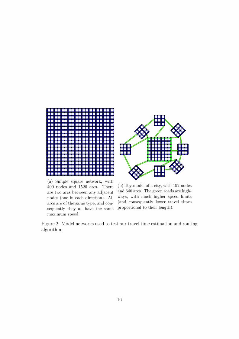
(a) Simple square network, with400 nodes and 1520 arcs. Thereare two arcs between any adjacentnodes (one in each direction). Allarcs are of the same type, and con-sequently they all have the samemaximum speed.

(b) Toy model of a city, with 192 nodesand 640 arcs. The green roads are high-ways, with much higher speed limits(and consequently lower travel timesproportional to their length).

Figure 2: Model networks used to test our travel time estimation and routingalgorithm.

16

destination pairs in V 2. In practice, taxi trips are not uniformly distributedover the city network; however, we will see in the Section 5 that our modelperforms well with real-world observations that are far from being uniformlydistributed. Then, Dod is chosen to be lognormal with log-mean parameterµ = log(T real

od ) and a second parameter σ that controls the randomness oftravel times from o to d. For context, Dod has geometric mean T real

od , anda value of σ = log 2 ≈ 0.7 means that a sampled time T i

od is within onegeometric standard deviation of the T real

od if it is between 0.5T realod and 2T real

od .The values T real

od are chosen to follow our shortest-path model. Therefore,we set a deterministic value of the parameter trealij for each arc (i, j), anddefine T real

od = minPod∈Pod

∑(i,j)∈Pod

trealij . As a consequence, T realod are the best

estimates of the distributions Dod given our shortest path model and theestimation loss introduced in Section 2.1.

We then use this process to sample N observations of origin-destinationtravel-times. For each (o, d) independently, we would need several samplesto be able to estimate T real

od (because of the randomness σ), but the routingnetwork model of our algorithm allows us to be able to use much less samplesto provide accurate point estimates for Dod (i.e. close to T real

od ), even when(o, d) 6∈ W .

4.2 Results

We evaluate the quality of our estimation using the Root Mean SquaredLog Error (RMSLE) of our estimates Tod, defined as the square root of theMSLE (1). Interestingly, the formulation simplifies when using the lognormaldistributions:

RMSLE(Tod) =

√σ2 + E(o,d)∼D

[(log(Tod)− log(T real

od ))2]

. (13)

To make it easier to compare our estimations across different values of σ, wefocus on the square root of the MSLB (RMSLB), removing the contributionof the log variance σ2 of the data ( see (3)).

RMSLB(Tod) =

√ ∑(o,d)∈V 2

(log(Tod)− log(T real

od ))2, (14)

where we used that D is uniform over V 2. Note that RMSLB = 0 meansthat we recover the geometric expectation of the travel times exactly.

We present the effects of our method when run on the city models de-scribed in the previous section, with a few different travel time functions and

17

Available amount of dataN = 100 N = 500 N = 1, 000 N = 10, 000

Randomness of input data RMSLB of estimation

σ = 0.0 0.08 0.03 0.01 0.01σ = 0.1 0.09 0.06 0.03 0.02σ = 0.5 0.23 0.12 0.15 0.05σ = 1.0 0.48 0.22 0.20 0.07σ = 2.0 0.62 0.43 0.30 0.15

Table 1: RMSLB (Root Mean Squared Log Bias) of estimation for a varyingamount of data and randomness σ. RMSLB of estimation for a varyingamount of data N and a varying amount of travel time randomness on the toycity model (see Fig. 2b). The toy city used has just under 37,000 node pairs(192 nodes), but notice that we need very little data to create an estimatewith small bias.

data generated as described above. We begin by studying the toy model ofa city introduced in Figure 2b. The values trealij are chosen by road type,with one speed for regular streets and another for the highways. We sampleN travel time observations as described in Section 4.1, and we start withrandom arc travel times to define the initial path P 0

od for each (o, d) in W .In Table 1 we present results of our method for different values of N and σ.

For all values of σ, when setting δ = 0.5 we find that the method tendsto converge in under 10 iterations. Each iteration on this small network (192nodes, 640 arcs) takes less than 10 seconds for a total run-time of less thantwo minutes. We noticed that the regularization term in the objective greatlyspeeds up convergence by reducing the relevance of tiny path differences.In addition, Table 1 confirms the rather obvious fact that results are moreaccurate with more data and less randomness in the data (top left corner).However, it also reveals that when the input has a high log variance σ2 it ispossible to obtain an estimate with comparatively small bias with very littledata. For example, when σ = 2, it is possible to obtain an estimation biasthat is smaller by more than a factor of two with only 100 observations, i.e.,less than 2% of the total origin-destination pairs.

The results in Table 1 should be taken with a grain of salt, however, asthe toy model in Fig. 2b is intentionally suited to the assumptions with whichwe developed our model (especially the velocity continuity assumption of ourregularization). The goal of this experiment is simply to confirm that themethod converges as intended and produces sensible results. The next step

18

(a) True congestion. (b) Reconstruction.

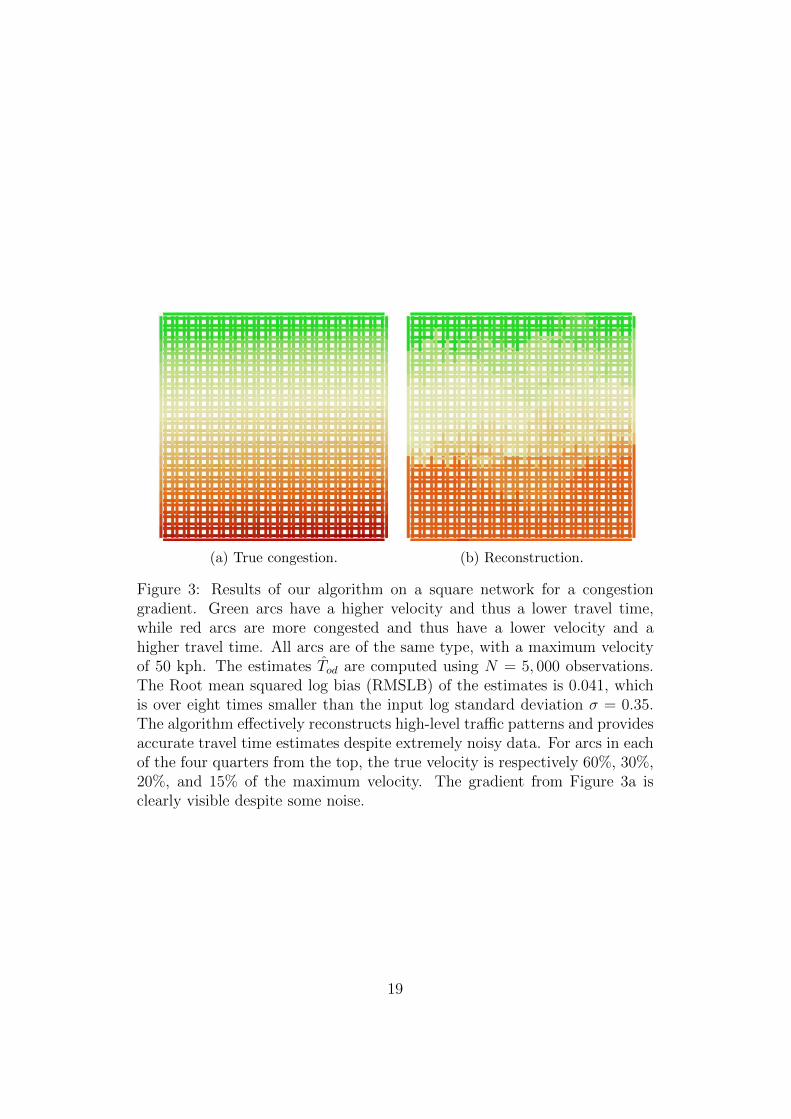
Figure 3: Results of our algorithm on a square network for a congestiongradient. Green arcs have a higher velocity and thus a lower travel time,while red arcs are more congested and thus have a lower velocity and ahigher travel time. All arcs are of the same type, with a maximum velocityof 50 kph. The estimates Tod are computed using N = 5, 000 observations.The Root mean squared log bias (RMSLB) of the estimates is 0.041, whichis over eight times smaller than the input log standard deviation σ = 0.35.The algorithm effectively reconstructs high-level traffic patterns and providesaccurate travel time estimates despite extremely noisy data. For arcs in eachof the four quarters from the top, the true velocity is respectively 60%, 30%,20%, and 15% of the maximum velocity. The gradient from Figure 3a isclearly visible despite some noise.

19

(a) True congestions (b) Reconstruction

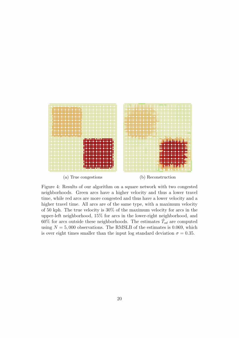
Figure 4: Results of our algorithm on a square network with two congestedneighborhoods. Green arcs have a higher velocity and thus a lower traveltime, while red arcs are more congested and thus have a lower velocity and ahigher travel time. All arcs are of the same type, with a maximum velocityof 50 kph. The true velocity is 30% of the maximum velocity for arcs in theupper-left neighborhood, 15% for arcs in the lower-right neighborhood, and60% for arcs outside these neighborhoods. The estimates Tod are computedusing N = 5, 000 observations. The RMSLB of the estimates is 0.069, whichis over eight times smaller than the input log standard deviation σ = 0.35.

20

is to consider a model that does not follow our traffic assumptions as closely.We therefore focus on the square network (400 nodes), which we associatewith two traffic configurations, presented in Figures 3 and 4, corresponding tosemi-realistic scenarios, including a gradual north-to-south increase in traveltime (Fig. 3a), and two congested neighborhoods where arc travel times aredoubled and quadrupled (Fig. 4a) as compared to the rest of the city. Readerswill note that these scenarios break our road velocity continuity assumptionin different ways: the first because the velocities of neighboring vertical arcsare never equal, and the second because the borders between congested anduncongested areas are strongly discontinuous in terms of velocity.

For each of the two scenarios thus described, we sample N = 5, 000observations as described in Section 4.1, for σ = 0.35 (we choose this valuebecause it is approximately our estimate of the log standard deviation ofManhattan taxi travel time data).

The arc travel times found by our algorithm are shown in Figures 3b and4b. The algorithm does a remarkable job reconstructing the travel times inthe network given limited data. As noted above, the data provided was noisy(σ = 0.35), yet the RMSLB for the estimated travel times Tod over all (o, d)in W is 0.07 in one case and 0.04 in the other. Therefore, the algorithm notonly produces accurate travel times estimates for the origin-destination pairsfor which no data was available, it does so with minimal bias when comparedto the high randomness and sparsity of the travel time data. Notice that theregularization term in the objective, though based on a questionable trafficassumption, does not preclude us from reconstructing the arc travel timesas desired in both cases, though it does make it difficult to find the exactborder of the congested neighborhoods in one case, and the precise velocitygradient in the other.

All in all, the method developed in this paper is able to extract usefulinformation from high-variance inputs, and produces a network cost function,in the form of arc travel times, that is interpretable and can in turn be used forother applications in the network. In the following section, we show that allthe algorithm properties displayed in this section, namely low estimation biasdespite inputs with high randomness, and the production of an interpretablefinal solution, also hold in a real-world setting at much larger scales.

5 Performance on Real-World Data

So far, we have described, implemented and tested a methodology to solve thetravel time estimation and routing problem. We use a network formulationbecause we assume the only allowed origins and destinations are nodes in the

21

graph. However, real origin-destination data records vehicles’ starting andending points using GPS coordinates, which are continuous variables.

In this section, we first provide a bridge between the continuous anddiscrete problems in order to apply our method to real-world OD data, andpresent the results on data from New York City taxis. We then display theresults of our method for varying amounts of available data, showing thatour method provides both accurate travel time estimations throughout thenetwork and sensible routing information, for an interpretable understandingof traffic in the city.

5.1 A Large-Scale Data Framework

A major contribution of this paper is the ability to exploit a large datasetto solve the travel time estimation and routing problem for the real-worldnetwork of a large city. Providing a tractable method at this scale requires theconstruction of a substantial framework to handle large amounts of networkinformation and origin-destination data, allowing us to leverage big datainsights in solving a complex problem.

In order to solve the travel time estimation and routing problem in areal-world setting, it is necessary to overcome two major challenges. The firstdifficulty is to extract a network structure from a complex urban landscape,and specifically to identify a graph that is elaborate enough to capture most ofthe details of the city under study, but simple enough to tractably supportour network optimization methods. For this purpose, we use open-sourcegeographical data from the OpenStreetMap project. Its database providesa highly-detailed map of New York City, which we simplify by excludingwalkways and service roads, and removing nodes that do not represent theintersection of two or more roads. For the island of Manhattan, to whichwe restrict our problem, we obtain a strongly connected graph with 4324nodes and 9518 arcs. This network is quite large, and the tractability of ourmethod on a map of this size is itself a significant contribution of this paper:readers will realize that an algorithm seeking to estimate travel times in thisnetwork must consider over 18 million origin-destination pairs of nodes andat least that many shortest paths.

The second challenge is obtaining and cleaning real OD data. Data fromthe New York City Taxi and Limousine Commission for the years 2009-2016is freely available from NYCTLC (2016). A month’s worth of data (ap-proximately 2GB) contains information for over 12 million taxi trips (over400,000 a day). We perform all computations, network and data handlingusing the Julia programming language. Our method’s tractability is en-hanced by the use of the cutting-edge Julia for Mathematical Programming

22

(JuMP) interface by Lubin and Dunning (2015), which enables us to takeadvantage of top-of-the-line linear and second-order programming methods,as implemented by the commercial solvers Gurobi and Mosek. Therefore, ourframework can handle problem instances considering hundreds of thousandsof data points in the entirety of Manhattan.

The results presented in Sections 5.3 and 5.4 use taxi data from weekdaysin May 2016, in the time windows 9-11AM (morning), 6-8PM (evening), and3-6AM (night). We restrict the data to a single month to reduce the taxitrip variance. Smaller time windows also guarantee less noisy data, but atthe cost of fewer data points, and so we opt for a medium-sized window of afew hours. Our method therefore seeks to capture network patterns that areaveraged over the considered time window.

In order to eliminate extreme outliers, we ignore trips shorter than 30sand longer than 3 hours, trips connecting points that are less than 250mor more than 200km away, and trips which would require an average speedgreater than 110 kph or less than 2 kph to make sense. The existence of suchunrealistic trips is a consequence of the imperfection of the GPS sensors insidethe taxi meters. After this filtering step, we split the data into a training setcontaining about 415,000 trips and a testing set containing about 275,000trips. In the next section, we explain how we adapt this taxi data to ourdiscrete network-based framework.

5.2 Applying a Discrete Model to Real-World Data

The model described in Section 2 is discrete in space and static in time:it considers fixed traffic patterns during a given time window in a networkwhere the only possible start and end locations are intersections. In contrast,real-world data is continuous in time and space: a given taxi trip is associatedwith a start time and an end time recorded by a clock within the taxi meter,and with start and end locations that are recorded using often noisy GPSsensors. We therefore need to process the data a bit further for it to workwith our model.

In the database, each taxi trip is represented as a 6-tuple (xO, yO, xD, yD, tstart, ttOD),where xO and yO are the GPS coordinates of the origin, xD and yD are theGPS coordinates of the destination, tstart is the date and time of the begin-ning of the ride, and ttOD is the travel time of the taxi from its origin toits destination. We use tstart to assign taxi trips to time intervals of lengthτ , and consider only this time window, discarding all taxi trips that do notstart inside this interval. For taxi trips that do start within the interval, wedo not differentiate between different tstart values, so each trip is reduced tothe 5-tuple (xO, yO, xD, yD, ttOD).

23

The length τ of the time interval should be chosen based on the scope ofthe application. If the goal is static planning, we can select a large value ofτ (from a few hours to a few months), which will allow us to consider a largeamount of data, and estimate fixed travel time parameters over the intervalas accurately as possible. If the goal is short-term dynamic planning, we canpick a small value of τ , say 5 minutes, and use the small amount of data inthis interval to quickly estimate the travel time parameters, which we willonly assume to be valid for the next time interval.

In the discrete formulation presented in the previous sections, the inputof the method is a set of node pairs W , with a known (but possibly noisy)travel time Tod for each (o, d) in the set W . In the continuous problem, theinputs are position vectors (xO, yO, xD, yD) and associated travel times ttOD.We therefore need to project the continuous origin (xO, yO) and destination(xD, yD) onto the network to be able to use our discrete methods in thisreal-world setting.

There exist many methods of projecting continuous data onto a discretenetwork model (see recent work by Quddus and Washington (2015), Chenet al. (2014)); all our results were obtained by projecting each continuousorigin-destination pair (xO, yO, xD, yD) to the nearest node pair (o, d) usingthe Euclidean metric in R4. We can now apply our algorithm to real taxidata in Manhattan.

5.3 Evaluating Results at the Scale of the City

Accuracy. We have explained in this paper that real-world OD data hassignificant variance, originating from several main sources: the imprecisionof the data-gathering protocol, including potent “urban canyoning” effects inGPS data, as well as the inherent variance of traffic patterns (see Section 2.1).The latter source is especially important when the time window is long, as aconsequence of our static traffic modeling assumption.

As seen in Section 2, the mean squared log error (MSLE) decomposes intothe sum of the mean log variance of the data and the mean squared log biasof our estimate. On empirical data, we can only evaluate the MSLE using(4). In order to be able to evaluate the performance of our estimation, weneed to estimate the log variance of the travel time observations (2). Indeed,it is a lower bound on the MSLE of our estimate, and a low-bias estimatemust have an MSLE as close as possible to this lower bound.

For this purpose, we simply compare each taxi trip in the data to theaverage of the k trips closest to it, and compute the empirical log variancebetween the two values. This gives us an upper bound on the log varianceterm of the MSLE of our estimate. Because the dataset is quite large, this

24

bound is indicative, especially when we choose the value of k that minimizesit. For instance, this approach yields an input log variance of 0.312 = 0.10for the time window 9-11 AM. To understand the magnitude of this variance,consider a mean time of 20 minutes. A trip within one standard deviationof the mean could last any amount of time between 20e−0.31 = 14.7 minutesand 20e0.31 = 27.3 minutes.

We will measure the accuracy of our method by how close the MSLEof our estimate is to the log variance (2) of the data. This is a proxy forminimizing the mean squared log bias (3), which is what we did in Section 4when we new the distributions Dod. If the difference between the MSLE ofour estimations and the input log variance of the data is small, it means thatour estimations are very close to the geometric mean of the network traveltimes, and most of our error comes from the inherent variability of the taxitrips.

For tractability reasons, we restrict the size of the input node pairs setW to 100,000 (o, d) pairs. With |W | = 100, 000, the total computation atthe scale of Manhattan takes less than 2 hours. We choose the regularizationparameter λ = 1000, which is the value that minimized the MSLE in cross-validation. We note that the algorithm converges in 10 iterations withoutshowing noticeable cycling (the out-of-sample improves at each iteration).

It turns out that between 9 and 11 AM, the out-of-sample RMSLE ofour estimations is just over 0.36. This result means that our travel timeestimation error is barely worse than the inherent noise in the data, andour estimated travel times must therefore be very close to the geometricexpectation of the travel times throughout the network.

Interpretability. In addition to its accuracy, we argue that our methodprovides global insights about traffic patterns in New York. To show this, wecompare our results in Manhattan in the morning (9-11AM), in the evening(6-8PM) and at night (3-6AM). We show the edge travel times for these timewindows in Figures 5 and 6. The overall traffic patterns are easily identifiablein Figure 5, in particular the effect of the morning (and to a lesser extent,evening) commute in Midtown, as well as the congestion in the northern partof the island near the bridges connecting it to the mainland.

The results of our algorithm provide insights at a variety of scales: inaddition to displaying citywide effects such as the daily commute, they alsoreveal more subtle realities about traffic in New York: For example, whenlooking at Figures 6a and 6b, it is clear that crosstown (east-west) travelersare much more exposed to congestion than uptown-downtown (north-south)travelers, and that the highways on Manhattan’s eastern and western shores

25

(a) Morning (9-11AM)

(b) Evening (6-8PM) (c) Night (3-6AM)

Figure 5: Edge travel times in Manhattan estimated by our algorithm onweekdays in May 2016 in the morning, evening and at night. The color ofeach edge represents the speed along that edge as a percentage of the referencevelocity v0 = 13.85 kph (average velocity in Manhattan on weekdays). At thescale of the city, the algorithm clearly identifies morning commute congestionin Midtown and the Financial District, while at the scale of individual cityblocks, it confirms the empirically known fact that crosstown (east-west)traffic in Manhattan is much more congested than uptown-downtown (north-south) traffic.

26

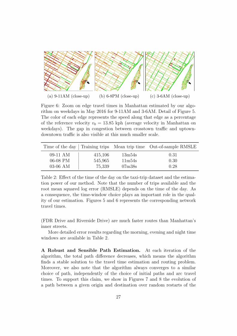
(a) 9-11AM (close-up) (b) 6-8PM (close-up) (c) 3-6AM (close-up)

Figure 6: Zoom on edge travel times in Manhattan estimated by our algo-rithm on weekdays in May 2016 for 9-11AM and 3-6AM. Detail of Figure 5.The color of each edge represents the speed along that edge as a percentageof the reference velocity v0 = 13.85 kph (average velocity in Manhattan onweekdays). The gap in congestion between crosstown traffic and uptown-downtown traffic is also visible at this much smaller scale.

Time of the day Training trips Mean trip time Out-of-sample RMSLE

09-11 AM 415,106 13m54s 0.3106-08 PM 545,965 11m54s 0.3003-06 AM 75,339 07m38s 0.28

Table 2: Effect of the time of the day on the taxi-trip dataset and the estima-tion power of our method. Note that the number of trips available and theroot mean squared log error (RMSLE) depends on the time of the day. Asa consequence, the time-window choice plays an important role in the qual-ity of our estimation. Figures 5 and 6 represents the corresponding networktravel times.

(FDR Drive and Riverside Drive) are much faster routes than Manhattan’sinner streets.

More detailed error results regarding the morning, evening and night timewindows are available in Table 2.

A Robust and Sensible Path Estimation. At each iteration of thealgorithm, the total path difference decreases, which means the algorithmfinds a stable solution to the travel time estimation and routing problem.Moreover, we also note that the algorithm always converges to a similarchoice of path, independently of the choice of initial paths and arc traveltimes. To support this claim, we show in Figures 7 and 8 the evolution ofa path between a given origin and destination over random restarts of the

27

algorithm. Specifically, we initiate the algorithm with random times: eachedge has a velocity drawn randomly between 1 and 130 kph. This results inthe random initial paths shown in panes 7a, 7b, and 7c. After 5 iterations,we consider the paths obtained by our method, in panes 8a, 8b, and 8c.

We see that in all three cases, the algorithm made the justifiable decisionof using the freeway on the western edge of Manhattan. In addition, despitestark differences in the starting point, the final paths found by the methodare eerily similar. One can quibble about the exact level of similarity betweenthese final paths, but it is wise to remember that our method does not seekto obtain the “optimal” path between an origin o and a destination d (andindeed Dial (1971) questions the existence of such an optimal path in anoisy environment), but simply a reasonable path that achieves the estimatedtravel time. Figure 8 is an example of our method accomplishing this statedpurpose.

To provide intuition for why our routes seem sensible, note that we haveempirically established that the travel time estimation accuracy in Manhat-tan has low bias, as we showed that the MSLE was close to our estimate ofthe mean log variance of the data. Additionally, the regularization allowsus to generalize well to parts of the city with few observations. Further-more, the obtained arc travel time parameters tij are good estimations onsynthetic data and seem reasonable in NYC. All these observations lead usto hypothesize that the obtained paths are sensible.

This result means that in a network with almost ten thousand nodes,with only a few OD pairs relative to the possible 18 million pairs, usinghigh variance data, we are able to reconstruct the all-pairs shortest pathsthat minimize the error between the shortest path lengths and the inputdata. Our optimization-based algorithm thus exhibits a certain number ofimportant properties: it is tractable at the scale of a large and complex city,produces accurate travel time estimations and sensible routing informationdespite high variance data, and produces an overall traffic map of the citythat can be used for numerous other applications. These results are obtainedwith a large number of data points, and in fact we operate at the limit ofwhat our solvers can handle. In the following section, we explore the effectof reducing available data on our method’s accuracy.

5.4 Impact of Data Density and Comparison with Data-Driven Methods

The results presented in Section 5.3 show that, when run with a large numberof data points, our method tractably estimates travel times in Manhattan.

28

(a) Random initial path1.

(b) Random initial path2.

(c) Random initial path3.

Figure 7: Evolution of paths studied by our algorithm : original paths. Threerandom starting point paths are presented. See Figure 8 for the results ofthe algorithm.

Given this performance with a wealth of data, it is natural to wonder howour algorithm fares when the data is much more sparse. Good performancein data-poor environments is important for two reasons: first, few cities haveas much demand for taxis as New York, so extending the method to othernetworks would necessitate good behavior with only minimal amounts ofdata. Second, taxis do not necessarily explore networks in a uniform manner:even in cities such as New York where they represent a significant fraction oftraffic, taxis only seldom visit certain neighborhoods, creating data-rich anddata-poor settings within a single network.

Nearest Neighbor Travel Time Estimation. In this section, we chooseto compare the performance of our method to simple purely data-drivenschemes, which are expected to work very well in a data-rich setting andcomparatively less well in a data-poor setting. Indeed, the formulation ofthe real-world travel time estimation problem as the estimation of ttOD asa function of the four variables xO, yO, xD, and yD suggests simple solutionapproaches based solely on the data. With no knowledge of the network orthe underlying behavior of taxi drivers, it is possible to use machine learningto infer travel times.

For instance, a simple k-nearest neighbors scheme would match an input

29

(a) Path 1 after 5 itera-tions.

(b) Path 2 after 5 itera-tions.

(c) Path 3 after 5 itera-tions.

Figure 8: Evolution of paths studied by our algorithm : path convergence.Shows the resulting path to which the algorithm converges after 5 iterations,starting from the initial paths and times presented in Figure 7. The readerwill notice that despite strong differences in the starting paths, the algorithmeventually converges to a very reasonable solution, a path that makes use ofthe freeway on the western shore of Manhattan.

30

origin and destination (xO, yO, xD, yD) ∈ R4 to the k taxi trips in the databaseclosest to it (for some choice of metric) and compute the geometric averageof their travel times to produce an estimate for the travel time between theprovided origin and destination.

This scheme has the advantage of being extremely simple and allowingfor quick travel time estimations. In addition, it is easy to see that the bias ofthis travel time estimate would converge to zero as the number of observationincrease (if k is scaled appropriately). Indeed, this approach is not limitedby the low-dimensional model assumption of our algorithm. However, inpractice it has several drawbacks: first, it is not particularly well suited totravel time estimation for origins and destinations for which little data isavailable. This is a particularly damaging flaw because, as stated before,origin-destination data is not very complete and is concentrated in regionswith more taxi traffic.

Second, this pure data-driven approach does not address the routing as-pect of the problem: with no knowledge of the network it cannot possiblyprovide information as to which path should be used. These two drawbacksjustify the use of our more complicated network optimization approach, butthe k-nearest neighbors scheme remains a useful benchmark of our perfor-mance. Of course, we do not expect to produce more accurate estimatesthan a k-nearest neighbors scheme when a wealth of taxi trips is available.With a good method, however, we should be able to obtain more accuratetravel times than k-nearest neighbors in zones without much data, and onlyslightly less accurate in zones where data is plentiful.

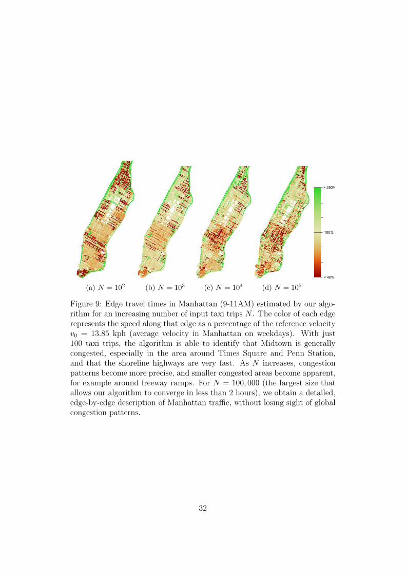
High Accuracy in Data-Poor Environments. To evaluate the impactof the dataset size on our method, we compute travel times and paths forvarying amounts of training data and compare the obtained RMSLE valueson the testing set with those produced by the k-nearest neighbors approach.We also compare our results to those produced by the travel time estima-tion method in Zhan et al. (2013) (for the small amounts of data where itis tractable). The results are presented in Table 3: though, as expected,the k-nearest neighbors scheme outperforms the optimization method forhigh amounts of data, it is significantly less accurate in a data-poor setting.Meanwhile, Zhan et al. (2013)’s method is less accurate and also untractablefor more than a small number of trips, as the runtime was 10-20 times longerthan ours (due to the much larger size of the network as compared to the oneused by the authors). Looking at the results, it seems that with our method,simply recording the origin, destination and travel time of 100 taxi trips isenough to accurately estimate the traffic patterns in an entire city.

31

(a) N = 102 (b) N = 103 (c) N = 104 (d) N = 105

100%

> 250%

< 40%

Figure 9: Edge travel times in Manhattan (9-11AM) estimated by our algo-rithm for an increasing number of input taxi trips N . The color of each edgerepresents the speed along that edge as a percentage of the reference velocityv0 = 13.85 kph (average velocity in Manhattan on weekdays). With just100 taxi trips, the algorithm is able to identify that Midtown is generallycongested, especially in the area around Times Square and Penn Station,and that the shoreline highways are very fast. As N increases, congestionpatterns become more precise, and smaller congested areas become apparent,for example around freeway ramps. For N = 100, 000 (the largest size thatallows our algorithm to converge in less than 2 hours), we obtain a detailed,edge-by-edge description of Manhattan traffic, without losing sight of globalcongestion patterns.

32

k-NN Optimization Zhan et al. (2013)Training trips Best k RMSLE Best λ RMSLE RMSLE

100,000 16 0.3243 1e3 0.3595 -10,000 11 0.3636 1e3 0.3775 -1,000 7 0.4296 1e3 0.4019 0.8228

100 6 0.5556 1e3 0.4495 0.8822

Table 3: Effect of data density on k-nearest neighbors (k-NN), our optimiza-tion method, and Zhan et al. (2013)’s method on the out-of-sample RMSLE.The best values of k and the continuity parameter λ are chosen. As be-fore, the convergence threshold δ is set to 0.5. For large amounts of data,k-nearest neighbors is unsurprisingly more accurate than our optimization-based method (although not by much), but it performs much worse in alow-data environment. Zhan et al. (2013)’s method is 10-20 times slowerthan ours (untractable for 10,000 trips or more), and is less accurate.

The accuracy gap between our method and k-nearest neighbors is notice-able, especially when you consider that our method also provides a path forany (o, d) pair in the network, which a simple k-nearest neighbors schemecan never provide since it has no knowledge of the network. Therefore, in adata-poor environment, our scheme is superior to a purely data-driven one interms of accuracy and routing, and both methods have a running time thatis appropriate for the application (a few seconds for k-nearest neighbors, afew minutes for our method). In a higher-data environment we pay for theadded routing information with a decrease in accuracy of just fractions of aminute and an increase in computational time.

6 Conclusions

The method proposed in this paper leverages a simple approach to tractablyyield accurate solutions to the travel time estimation and routing problem ina real-world setting. Given trip times for any number of origin-destinationpairs, from a few hundred to a few hundred thousand, we can estimate thetravel time from any origin to any destination, as well as provide a sensiblepath associated with this travel time. Furthermore, our algorithm is robustto a high degree of input uncertainty, successfully exploiting very noisy datato provide results characterized by their accuracy.

Providing travel times for each arc in the city effectively augments thenetwork with a cost function based on real traffic information, which can be

33

of use both for city planners and for further network-based research. Usingour optimization-based framework, we can estimate traffic patterns in a real-world network, providing insight at every scale, from a few blocks to theentire city, and extracting global meaning from the observed data.

Acknowledgement

We would like to thank the area editor Prof. Anton Kleywegt, the associateeditor and three reviewers for many careful and insightful comments thatimproved the paper significantly. Research funded in part by ONR grantsN00014-12-1-0999 and N00014-16-1-2786. Geographical data for New YorkCity is copyrighted to OpenStreetMap contributors and available from OSM(2015).

References

Chen BY, Yuan H, Li Q, Lam WHK, Shaw SL, Yan K (2014) Map-matchingalgorithm for large-scale low-frequency floating car data. Int. J. Geogr. Inf.Sci. 28(1):22–38.

Coifman B (2002) Estimating travel times and vehicle trajectories on freeways us-ing dual loop detectors. Transportation Research Part A: Policy and Practice36(4):351 – 364.

Dial RB (1971) A probabilistic multipath traffic assignment model which obviatespath enumeration. Transportation Research 5(2):83–111.

Hanseler F, Molyneaux N, Bierlaire M (2017) Estimation of pedestrian origin-destination demand in train stations. Transportation Science 51(3):981–997.

Hofleitner A, Herring R, Abbeel P, Bayen A (2012) Learning the dynamics ofarterial traffic from probe data using a dynamic bayesian network. IEEETransactions on Intelligent Transportation Systems 13(4):1679–1693.

Hung CH (2003) On the Inverse Shortest Path Length Problem. Ph.D. thesis, Geor-gia Tech ISyE.

Jaillet P, Qi J, Sim M (2016) Routing optimization under uncertainty. OperationsResearch 64(1):186–200.

Jenelius E, Koutsopoulos HN (2013) Travel time estimation for urban road net-works using low frequency probe vehicle data. Transportation Research PartB: Methodological 53:64 – 81.

Li R, Rose G (2011) Incorporating uncertainty into short-term travel time predic-tions. Transportation Research Part C: Emerging Technologies 19(6):1006 –1018.

34

Lubin M, Dunning I (2015) Computing in operations research using julia. IN-FORMS Journal on Computing 27(2):238–248.

Nikolova E, Stier-Moses NE (2014) A mean-risk model for the traffic assignmentproblem with stochastic travel times. Operations Research 62(2):366–382.

NYCTLC (2016) Trip record data. http://www.nyc.gov/html/tlc/html/about/trip_record_data.shtml.

OSM (2015) OpenStreetMap Project Database. http://planet.openstreetmap.org.

Pioro M, Fouquet Y, Nace D, Poss M (2016) Optimizing flow thinning protectionin multicommodity networks with variable link capacity. Operations Research64(2):273–289.

Quddus M, Washington S (2015) Shortest path and vehicle trajectory aided map-matching for low frequency GPS data. Transportation Research Part C:Emerging Technologies 55:328 – 339.

Santi P, Resta G, Szell M, Sobolevsky S, Strogatz S, Ratti C (2014) Quantifyingthe benefits of vehicle pooling with shareability networks. Proceedings of theNational Academy of Sciences 111(37):13290–13294.

Wang H, Li Z, Kuo Y, Kifer D (2015) A simple baseline for travel time estimationusing large-scale trip data. CoRR abs/1512.08580.

Wang Y, Nihan NL (2000) Freeway Traffic Speed Estimation Using Single LoopOutputs. Transportation Research Record: Journal of the Transportation Re-search Board 1727(1):9.

Wang Y, Zheng Y, Xue Y (2014) Travel time estimation of a path using sparsetrajectories. Proceedings of the 20th ACM SIGKDD International Conferenceon Knowledge Discovery and Data Mining, 25–34 (KDD 2014).

Yang C (2015) Data-driven modeling of taxi trip demand and supply in New YorkCity. Ph.D. thesis, Rutgers University.

Zhan X, Hasan S, Ukkusuri SV, Kamga C (2013) Urban link travel time estimationusing large-scale taxi data with partial information. Transportation ResearchPart C: Emerging Technologies 33:37 – 49.

35