tree automata - carnegie mellon school of computer scienceneelk/tree-automata.pdf · why tree...

Tree Automata

Neel Krishnaswami

Department of Computer ScienceCarnegie Mellon University

Why Tree Automata?

• Type declarations with refinement types declare a latticeof subtypes of an ML datatype.

• The ∨ and ∧ operators in the type algebra create newentries in the lattice.

• Once we get such a type, we need to get the least upperbound of the type in the declared subtype lattice to figureout which refinement it is.

• Tree Automata and regular tree grammars describe setsof trees, and have well known (if exponential worst-case)algorithms for testing inclusion.

15-819: Type Refinements for Programming Languages

1

What Will Be Discussed

• Tree automata

• Tree grammars

• Implementation


2

Preliminaries: Ranked Alphabets

A ranked alphabet F consists of an alphabet∑

and a function

a :∑→ N. Examples are x, y, nil, sin/1, cons/2.

Arity-0 terms are written without the explicit arity marker.

Fi refers to {x ∈ F|a(x) = i}.


3

Preliminaries: Trees

Assume the existence of a set of constants X such that Fand X are disjoint. Then define the set of trees T(F ,X ) as

the least set defined by:

• F0 ⊆ T(F ,X )

• X ⊆ T(F ,X )

• f(t1, · · · , tn) ∈ T(F ,X ) if n ≥ 1, t1 · · · tn ∈ T(F ,X ), and f ∈Fn


4

Preliminaries: Ground Terms and Substitutions

• A term t is ground if no x ∈ X appear in it, and the setof all ground terms T(F , ∅) is written T(F).

• A term with variables is called linear if each variable ap-pears at most once.

• A substitution is a mapping σ : X → T(F), with a finitedomain.

• Let Xn be a set of n variables. A context is a linear termC ∈ T(F ,Xn). We write C[t1, · · · ,1n] to mean σ(C), whereσ = {t1 ← x1, · · · , tn ← xn}, and C(F) for all contexts overF.


5

Bottom-up Tree Automata, Defined

A tree automaton is a tuple A = (Q,F , Qf ,∆), where Q is

a set of states, the final states Qf ⊆ Q, and ∆ is a relation

whose elements are written like this: f(q1, · · · , qn) → q, with

n = a(f).


6

The Transition Relation

The transition relation t→A t′ is defined by:

t→A t′ ⇔

∃C ∈ C(F ∪Q),∃f(q1, · · · , qn)→ q ∈∆,t = C[f(q1, · · · , qn)],t′ = C[q]


7

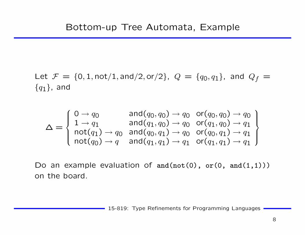
Bottom-up Tree Automata, Example

Let F = {0,1,not/1, and/2,or/2}, Q = {q0, q1}, and Qf =

{q1}, and

∆ =

0→ q0 and(q0, q0)→ q0 or(q0, q0)→ q01→ q1 and(q1, q0)→ q0 or(q1, q0)→ q1not(q1)→ q0 and(q0, q1)→ q0 or(q0, q1)→ q1not(q0)→ q and(q1, q1)→ q1 or(q1, q1)→ q1

Do an example evaluation of and(not(0), or(0, and(1,1)))

on the board.


8

Various Properties

Many properties of bottom-up regular tree automata have

analogues with string automata:

• Nondeterministic automata can be made deterministic

with a subset construction, just like string automata.

• There’s a pumping lemma, only it works on the height of

trees, rather than the length of the string.

• Deterministic automata can be minimized, using a version

of the Myhill-Nerode theorem generalized to trees.


9

Top-down Tree Automata

Nodeterministic top down tree automata are just like bottom-

up tree automata, except that the final set Qf gets replaced

with an initial set Qi, and the transitions change to the form:

q(f(x1, . . . , xn))→ f(q1(x1), . . . , qn(xn))


10

Deterministic Top Down Automata Are Weaker

However, deterministic top-down automata recognize a smaller

set of languages. For example, consider L = {f(a, b), f(a′, b′)}.If you try to construct a top-down deterministic automaton,

you run into the problem that the rule for the function sym-

bol f is of the form q(f(x1, x2)) → f(q1(x1), q2(x2)). So the

state q1 must recognize both a and a′, and likewise for q2. So

the smallest language L′ a top-down deterministic automaton

containing L must be {f(a, b), f(a′, b), f(a, b′), f(a′, b′)}.

This is what leads to the tuple distributivity restriction in the

Yardeni and Shapiro paper.


11

Closure properties

Recognizable tree languages are closed under complementa-

tion, union, and intersection. I won’t offer the proofs, but

will describe the constructions used.

To get the complement language, start with a deterministic

automaton for it, and then swap the final and non-final states.

This is possibly exponential if you start with an NFTA, as

usual.

Union and intersection can be found using product automata


12

Product Automata for Union and Intersection

Suppose you have two automata A1 = (Q1,F , Qf1,∆1) and

A2 = (Q2,F , Qf2,∆2), which recognize languages L(A1) and

L(A2). To construct a product automaton, let:

Q′ = Q1 ×Q2

∆′ =

{f((q11, q21), . . . , (q

1n, q2n))→ (q1, q2)|

f(q11, · · · , q1n)→ q1 ∈∆1,

f(q21, · · · , q2n)→ q2 ∈∆2

}

For union, let Q′f = (Q1f × Q2) ∪ (Q1 × Q2f), and for inter-

section let Q′f = Q1f ×Q2f .


13

Complexity of Decision Problems

• Testing membership is linear in the size of the term t.

• Testing the emptiness of the language an automaton A

recognizes takes time proportional to |A|. (The trick is

to compute the set of reachable states and then to see

if any of them are in the final set.)


14

Complexity of Decision Problems

• The finiteness of the accepted language can be checked

in time proportional to |A|, by checking for loops in the

transition rules.

• An inclusion algorithm is easy to get since we have clo-

sure under intersection, union and complement, and an

emptiness test. Unfortunately, this is potentially expo-

nential time for NFTAs.


15

Regular Tree Grammars

A regular tree grammar G = (S, N,F , R) is given by an axiom

S, a set of non-terminals N (with S ∈ N), and a set of

production rules A→ α, where A ∈ N and α ∈ T(F ∪N).

Example:

List → nilList → cons(Nat, List)Nat → 0Nat → succ(Nat)


16

Normalized Tree Grammars

A normalized regular tree grammar is a tree grammar in which

all of the production rules are of the form A→ f(A1, . . . , An)

or A → a, where the Ai are nonterminals and the f, a are

elements of F. Every regular tree grammar can be con-

verted into a normalized tree grammar, by first discarding

all the non-productive and non-reachable nonterminals, and

then introducing new nonterminals for nested productions.


17

Equivalence of Automata and Tree Grammars

Given a normalized grammar G = (S, N,F , R), we can con-

struct a tree automaton to recognize it as follows:

Q = {QA|A ∈ N}Qf = QSf(qA1

, . . . , qAn)→ qA ∈∆ if and only if A→ f(A1, . . . , An) ∈ R

Likewise for the other direction.


18

Algorithms for Fast Automata Operations

The main tricks that Aiken and Murphy use in their imple-mentation are:

• Maintain the system in a form close to a normalized treegrammar (or an NFTA), rather than in a determinis-tic form, in order to avoid potential exponential spacegrowth.

• Maintaining the rules in a form that enables fast empti-ness tests.

• Maintaining the rules in a form that enables “fast” nega-tion.


19

Representation Tricks: Leaf-linear form

Aiken and Murphy maintain their regular tree language in a

form they call leaf-linear form. This is essentially a variation

of a normalized regular tree grammar. First, they add two

special terminal symbols – 0 and 1. 0 matches no terms, and

1 matches all ground terms. (Their syntax also apparently

permits conjunctions, but that’s an illusion.)


20

Fast emptiness tests

Aiken and Murphy maintain the invariant that whenever a

particular production rule generates the empty set, it shall be

represented with the 0 symbol. This makes testing emptiness

an O(1) operation, though they have maintain the invariant

(which they do by simplifying expressions until they can be

sure they are 0).

Taking the union of two leaf-linear systems that maintain

the emptiness invariant is trivial; simply add the new equa-

tions Snew = S1 and Snew = S2. Maintaining the emptiness

requirement is a trivial check.


21

Fast emptiness tests: Intersection

Intersection is a lot harder; its worst-case time is exponential,

since there is no choice but to use the product construction.

However, Aiken and Murphy found it possible to do better

in the average case. They took a system of equations with

axioms S1 and S2, and then defined S′ = S ∪ {x = Simp(S1 ∧S2)}, and then simplified the set of equations. At the last

step, they identified all of the terms xi ∧ xj and introduced

new variables for them.


22

Fast emptiness tests: Negation

Aiken and Murphy report that tree negation does suffer from

exponential blowup in practice. They deal with this problem

by using a conservative approximation to negation (whether

this is a subset or superset depends on the problem for which

the answer will be used). After propagating the negation for

some number of steps k through the set of equations, they

simpy returned either 0 or 1, depending.

Question: Do refinement types ever generate negations? It

looked like they don’t, but I didn’t fully understand Frank’s

talk last week.


23

Inclusion

I am not sure their inclusion test results are relevant to re-

finement types. They are trying to solve a very different

decision problem from the one that arises in refinement type-

checking. Aiken and Murphy want to solve ∀σ.σ(S1) ⊆ σ(S2)

and ∃σ.σ(S1) ⊆ σ(S2), where S1 and S2 can contain variables.


24

Other optimizations

The main other optimization they used was simply memoizing

any of the tree operations, and maintaining the memos in one

hash table for each operation.


25

Correction

The relationship between context-free grammars and tree au-

tomata is more complicated than I suggested: for any tree

automaton, the fringe of its trees can be recognized by a

context-free grammar, and vice versa.

The set of trees themselves is bigger; for example, they can

be used to decide temporal logic propositions.


26

Algebraic Definition of Tree Automata

An F-algebra is a pair A = (Q, α), where Q is a set (called

the carrier of A) and α is a function that assigns to each

f ∈ F a function αf : Qarity(f) → Q. (F is the usual ranked

alphabet.)


27

Homomorphisms on F-algebras

Suppose that σ : X → Q is an assignment of variables to

elements of the carrier. This determines a unique homomor-

phism hσ from T(F ,X ) into Q:

• hσ(x ∈ X ) = σ(x)

• hσ(a ∈ F0) = αa

• hσ(f(t1, . . . , tn)) = αf(hσ(t1), . . . , hσ(tn)) where f ∈ Fn

Clearly, all hσ are the same on all ground terms; we write hAto restrict the domain to ground terms.


28

Tree Automata Defined

A tree automaton A can be seen as a pair (A, Qf), where Ais an F-algebra and Qf ⊆ Q, and |Q| is finite.

A ground term t is accepted if hA ∈ Qf .


29

Algebra and Substitution

The big win to thinking in algebraic terms is that we can

easily change the carrier from “states” to any other set. For

example, take Q to be a finite subset of T(F ,X ), and the

unique homomorphism on the algebra defines substitution

for us.


30

Linear homomorphisms∗

A linear homomorphism g is a mapping for each f ∈ F to a

linear term tf ∈ T(F ′,Xarity(f)), extended to trees such that:

• g(a) = ta for a ∈ F0

• g(f(t1, . . . , tn)) = tf{x1 ← g(t1), . . . , xn ← g(tn)}

* These are called pure finite-state transforms in the Thatcher paper I

got the proof from.


31

Proof of closure under linear homomorphisms

Automata languages are closed under linear homomorphisms.

That is, given an automaton A = (A, Qf), and a linear ho-

momorphism g, the image of the language recognized by A,

g(L(A)) is also a recognizable language.


32

Sketch of Proof

Suppose we have an automaton A = (Q,F , Qf ,∆) which rec-

ognizes a language L(A). We can construct an automa-

ton to recognize g(L(A)) using the following construction

A′ = (Q′,F ′, Q′f ,∆′). We get ∆′ using the following proce-

dure: consider each rule f(q1, . . . , qn)→ q ∈∆, and the linear

term tf . We define a set of states Qr = {qrp|p ∈ Pos(tf)}, and

for all positions p:

tf(p) = f ′ ∈ F ′k ⇒ f ′(qrp1, . . . , qr

pk)→ qrp ∈∆r

tf(p) = xi ⇒ qi → qrp ∈∆r

qrε → q ∈∆r


33

Sketch of Proof

• Q′ = Q ∪⋃

r∈∆ Qr

• Q′f = Qf

• ∆′ =⋃

r∈∆ ∆r

You can then do an induction on the reduction to get the

desired result. This proof depends critically on the linearity

assumption!


34

tree automata - carnegie mellon school of computer scienceneelk/tree-automata.pdf · why tree...

Documents