tree-structured like representations for … like representations for continuous and graph indexed...
TRANSCRIPT
Tree-Structured Like Representations for Continuous
and Graph Indexed Markov Random Fields
Submitted in partial fulfillment of the requirements for
the degree of
Doctor of Philosophy
in
Electrical and Computer Engineering
Divyanshu Vats
B.S., Mathematics, The University of Texas at AustinB.S., Electrical Engineering, The University of Texas at Austin
M.S., Electrical and Computer Engineering, Carnegie Mellon University
Carnegie Mellon University
Pittsburgh, PA
May, 2011

ii

Abstract
Markov random fields (MRFs) are ubiquitous models for conveniently capturing com-
plex statistical dependencies given a collection of random variables. For example, when
modeling the temperature distribution of a continuously indexed region, it is common to
assume that the temperature at one point depends on some differential neighborhood.
MRFs can capture such dependencies using a set of conditional independence relation-
ships and thereby lead to compact representations of random signals. Other examples of
using MRFs is when modeling a finite collection of gene expressions or when modeling
pixel intensities in images.
Although MRFs lead to compact representations for high-dimensional spatially vary-
ing random signals, the resulting representations are often noncausal and thus standard
recursive algorithms popular for processing causal signals (temporal signals) can no longer
be applied. The central theme of this thesis is to find alternate representations in arbi-
trary MRFs in the form of a tree so that standard recursive algorithms, like the Kalman
filter and the belief propagation algorithm, for trees can be applied to MRFs. We study
two kinds of MRFs in this thesis: (i) MRFs indexed over high-dimensional continuous
indices, and (ii) MRFs indexed over graphs.
For MRFs indexed over high-dimensional continuous indices, we show that, a natural
tree-structured like representation, in this case a chain, exists on a collection of hypersur-
faces embedded in the continuous index set. For Gaussian MRFs, this leads to telescoping
representations in the form of a linear stochastic differential equation that initiates at the
boundary of the MRF and recurses inwards in a telescoping manner. Using the telescop-
iii

ing representation, we derive algorithms for recursively processing random signals indexed
over continuous domains.
For MRFs indexed over graphs (commonly referred to as graphical models,) where
the edges in the graph capture various conditional independence relationships among
random variables, we show that a tree-structured like representation can be derived by
appropriately clustering nodes in the graph so that the graph over the clusters is a tree.
We call the resulting graph a block-tree. Like the telescoping representation for MRFs
indexed over continuous indices, the block-tree representation leads to algorithms for
recursive processing of graphical models. Using the block-tree representation, we propose
a framework for generalizing common algorithms over graphical models. As an example,
we show how block-trees can be used to perform generalized belief propagation over
graphical models to obtain more accurate inference algorithms.
iv

Acknowledgment
I would like to thank my advisor, Prof. Jose M. F. Moura, for his guidance, support, and
encouragement during these past five years at Carnegie Mellon University. Prof. Moura
has been a continuous source of knowledge and passion that I can only hope to emulate
someday. Not only has he given me constant feedback on various research paper drafts
and presentations, which I know will help me in my future research and academic pursuits,
but he has also guided and given me the freedom to pursue various research problems of
my own interest.
I would like to thank my thesis committee members Prof. Vijayakumar Bhagavatula,
Prof. Rohit Negi, Prof. Markus Puschel, Prof. Bernard Levy, and Dr. Ta-Hsin Li for all
their valuable feedback on my thesis research that helped me channelize my thoughts and
shape my research ideas. I thank Prof. Levy for agreeing to be on my committee on such
notice and also for his papers on reciprocal processes and Markov random fields. I thank
Prof. Negi for allowing me to be his teaching assistant on two occasions and guiding me
through the tricky task of creating homework and exam problems.
I would like to thank Prof. Brian Evans and Prof. Joydeep Ghosh from UT Austin
and Prof. Richard Baraniuk from Rice University for supporting my graduate school
applications. I thank Prof. Evans for introducing me to research and for advising me as
an undergraduate student. I thank Prof. Baraniuk for giving me the opportunity to work
at Rice University as an undergraduate student and introducing me to various research
problems. I thank Vishal Monga for guiding me as an undergraduate student and again
as a graduate student when I spent a summer working at Xerox Research.
v

I would like to thank my office mates Kyle Anderson, Aurora Schmidt, Marek Telgar-
sky, Soummya Kar, and Dusan Jakovetic for all the insightful discussions on both research
and non-research related topics. In addition to my office mates, I would like to thank
my fellow ECE students Aliaksei Sandryhaila, Frederic de Mesmay, Joel Harley, Nicholas
ODonoughue, James Weimer, Joao Mota, Augusto Santos, Joya Deri, and June Zhang
for their helpful feedback on departmental presentations and the discussions on various
research topics. I would like to thank Carol Patterson for all the logistical help. I thank
the ECE Graduate Organization (EGO) for organizing various social events throughout
the year.
I would like to thank my friends from Austin and Pittsburgh for making life enjoyable
outside the office. I thank my in-laws and sister-in-law for all their encouragement and
support. I thank my parents for encouraging me to pursue my passions and always
supporting me in my endeavors. I thank them for teaching me the value of education
and I hope to someday be the educator and researcher that they are. I thank my sister
for all her encouragement and support. Finally, this thesis would not have been possible
without the love and support of my wife. I thank her for being patient with me as I
worked towards this thesis. I thank her for helping me get through some tough times. I
thank her for listening to my research ideas and pointing me to relevant references. Most
importantly, I thank her for teaching me to have a dream.
The work in this thesis was supported in part by DARPA under award HR0011-05-1-
0028.
vi
Contents
Abstract ii
Acknowledgment iv
1 Introduction 1
1.1 Motivation . . . . . . . . . . . . . . . . . . . . . . . . . . . . . . . . . . . . . . . 1
1.2 Markov Random Fields Over Continous Indices . . . . . . . . . . . . . . . . . . . 2
1.2.1 Literature Review . . . . . . . . . . . . . . . . . . . . . . . . . . . . . . . 2
1.2.2 Summary of Contributions . . . . . . . . . . . . . . . . . . . . . . . . . . 4
1.3 Markov Random Fields Over Graphs . . . . . . . . . . . . . . . . . . . . . . . . . 5
1.3.1 Literature Review . . . . . . . . . . . . . . . . . . . . . . . . . . . . . . . 5
1.3.2 Summary of Contributions . . . . . . . . . . . . . . . . . . . . . . . . . . 6
1.4 Thesis Summary and Organization . . . . . . . . . . . . . . . . . . . . . . . . . . 7
1.5 Bibliographical Notes . . . . . . . . . . . . . . . . . . . . . . . . . . . . . . . . . . 8
2 Telescoping Representations for Continuous Indexed Markov Random Fields 9
2.1 Introduction . . . . . . . . . . . . . . . . . . . . . . . . . . . . . . . . . . . . . . . 9
2.1.1 Summary of Contributions . . . . . . . . . . . . . . . . . . . . . . . . . . 10
2.1.2 Related Work . . . . . . . . . . . . . . . . . . . . . . . . . . . . . . . . . . 11
2.1.3 Chapter Organization . . . . . . . . . . . . . . . . . . . . . . . . . . . . . 12
2.2 Gauss-Markov Random Fields . . . . . . . . . . . . . . . . . . . . . . . . . . . . . 13
2.3 Telescoping Representation: GMRFs on a Unit Disc . . . . . . . . . . . . . . . . 17
2.3.1 Main Theorem . . . . . . . . . . . . . . . . . . . . . . . . . . . . . . . . . 18
2.3.2 Homogeneous and Isotropic GMRFs . . . . . . . . . . . . . . . . . . . . . 22
vii
CONTENTS
2.4 Telescoping Representation: GMRFs on arbitrary domains . . . . . . . . . . . . . 25
2.4.1 Telescoping Surfaces Using Homotopy . . . . . . . . . . . . . . . . . . . . 25
2.4.2 Generating Similar Telescoping Surfaces . . . . . . . . . . . . . . . . . . . 28
2.4.3 Telescoping Representations . . . . . . . . . . . . . . . . . . . . . . . . . . 29
2.5 GMRFs Pinned to Two Boundaries . . . . . . . . . . . . . . . . . . . . . . . . . . 30
2.6 Recursive Estimation of GMRFs . . . . . . . . . . . . . . . . . . . . . . . . . . . 33
2.7 Summary . . . . . . . . . . . . . . . . . . . . . . . . . . . . . . . . . . . . . . . . 36
3 Block-Tree Structures in Markov Random Fields Over Graphs 37
3.1 Introduction . . . . . . . . . . . . . . . . . . . . . . . . . . . . . . . . . . . . . . . 37
3.2 Background and Problem Statement . . . . . . . . . . . . . . . . . . . . . . . . . 39
3.2.1 Graphs and Graphical Models . . . . . . . . . . . . . . . . . . . . . . . . . 39
3.2.2 Inference Algorithms . . . . . . . . . . . . . . . . . . . . . . . . . . . . . . 42
3.2.3 Belief Propagation . . . . . . . . . . . . . . . . . . . . . . . . . . . . . . . 44
3.2.4 Junction-Tree . . . . . . . . . . . . . . . . . . . . . . . . . . . . . . . . . . 45
3.2.5 Problem Statement . . . . . . . . . . . . . . . . . . . . . . . . . . . . . . . 51
3.3 Tree Structures in Graphs Using Block-Trees . . . . . . . . . . . . . . . . . . . . 52
3.3.1 Constructing Block-Trees . . . . . . . . . . . . . . . . . . . . . . . . . . . 52
3.3.2 A Linear Time Block-Tree Construction Algorithm . . . . . . . . . . . . . 56
3.3.3 Block-Trees Vs. Junction-Trees . . . . . . . . . . . . . . . . . . . . . . . . 57
3.4 Inference of Graphical Models Using Block-Trees . . . . . . . . . . . . . . . . . . 58
3.4.1 Belief Propagation on Block-Trees . . . . . . . . . . . . . . . . . . . . . . 58
3.4.2 Optimal Block-Trees . . . . . . . . . . . . . . . . . . . . . . . . . . . . . . 60
3.4.3 Greedy Algorithms For Finding Optimal Block-Trees . . . . . . . . . . . . 61
3.5 Inference Over Graphical Models: Block-Tree Vs. Junction-Tree . . . . . . . . . 63
3.5.1 Example: Single Cycle Graphical Models . . . . . . . . . . . . . . . . . . 63
3.5.2 Example: Erdos-Renyi Graph . . . . . . . . . . . . . . . . . . . . . . . . . 64
3.5.3 Discussion . . . . . . . . . . . . . . . . . . . . . . . . . . . . . . . . . . . . 65
3.6 Summary . . . . . . . . . . . . . . . . . . . . . . . . . . . . . . . . . . . . . . . . 66
viii
CONTENTS
4 Generalizing Algorithms on Graphical Models Using Block-Graphs 69
4.1 Introduction . . . . . . . . . . . . . . . . . . . . . . . . . . . . . . . . . . . . . . . 69
4.2 Generalized Algorithms Using Block-Graphs . . . . . . . . . . . . . . . . . . . . . 71
4.2.1 General Theory . . . . . . . . . . . . . . . . . . . . . . . . . . . . . . . . . 72
4.2.2 Approximate Inference Using Block-Graphs . . . . . . . . . . . . . . . . . 73
4.3 Constructing Block-Graphs . . . . . . . . . . . . . . . . . . . . . . . . . . . . . . 74
4.4 Numerical Simulations . . . . . . . . . . . . . . . . . . . . . . . . . . . . . . . . . 76
4.5 Related Work . . . . . . . . . . . . . . . . . . . . . . . . . . . . . . . . . . . . . . 79
4.6 Summary . . . . . . . . . . . . . . . . . . . . . . . . . . . . . . . . . . . . . . . . 81
5 Conclusion and Future Work 83
5.1 List of Contributions . . . . . . . . . . . . . . . . . . . . . . . . . . . . . . . . . . 83
5.2 Chapter Summaries . . . . . . . . . . . . . . . . . . . . . . . . . . . . . . . . . . 84
5.2.1 Chapter 2: Tree-Structures in MRFs over Continuous Indices . . . . . . . 84
5.2.2 Chapter 3: Block-Tree Structures in MRFs over Graphs . . . . . . . . . . 85
5.2.3 Chapter 4: Generalizing Algorithms on Graphical Models . . . . . . . . . 85
5.3 Suggestions for Future Work . . . . . . . . . . . . . . . . . . . . . . . . . . . . . 86
5.3.1 Estimation of Random Fields Over Continuous Indices . . . . . . . . . . . 86
5.3.2 Other Applications of Using Block-Graphs . . . . . . . . . . . . . . . . . . 86
5.3.3 Learning Graphical Models Using Block-Graphs . . . . . . . . . . . . . . 87
A Appendix to Chapter 2 89
A.1 Computing bj(s, r) in Theorem 2.2.1 . . . . . . . . . . . . . . . . . . . . . . . . . 89
A.2 Proof of Theorem 2.3.1: Telescoping Representation . . . . . . . . . . . . . . . . 92
A.3 Proof of Theorem 2.6.1: Recursive Filter . . . . . . . . . . . . . . . . . . . . . . . 96
A.4 Proof of Theorem 2.6.2: Recursive Smoother . . . . . . . . . . . . . . . . . . . . 102
Bibliography 118
ix

CONTENTS
x

List of Figures
1.1 Conditional independence relationships for Markov processes (left), reciprocal
processes (middle), and Markov random fields (right). For a Markov process,
the past ⊥ future | present. For reciprocal processes and Markov random fields,
interior ⊥ exterior | boundary. . . . . . . . . . . . . . . . . . . . . . . . . . . 3
1.2 Examples of hypersurfaces on which we derive recursive representations. In
(a),(b), and (c) we have have hypersurfaces for a field defined on a dics. In (d),
we have surfaces defined on an arbitrary region. . . . . . . . . . . . . . . . . . 4
1.3 Examples of various graphical models and a graphical model defined on a block-
tree. . . . . . . . . . . . . . . . . . . . . . . . . . . . . . . . . . . . . . . . 5
2.1 Different kinds of telescoping recursions for an MRF defined on a disc. . . 10
2.2 (a) An example of complementary sets on a random field defined on S with
boundary ∂S. (b) Corresponding notion of complementary sets for a random
process. . . . . . . . . . . . . . . . . . . . . . . . . . . . . . . . . . . . . . . 14
2.3 A random field defined on a unit disc. The boundary of the field, i.e., the field
values defined on the circle with radius 1 is denoted by x(∂S). The field values
at a distance of 1 − λ from the center of the field are given by x(∂Sλ). Each
point is characterized in polar coordinates as xλ(θ), where 1− λ is the distance
to the center and θ denotes the angle. . . . . . . . . . . . . . . . . . . . . . . 18
2.4 Telescoping surfaces defined using different homotopies. . . . . . . . . . . . . . 26
2.5 Telescoping surfaces defined using different homotopies on arbitrary regions. . . 29
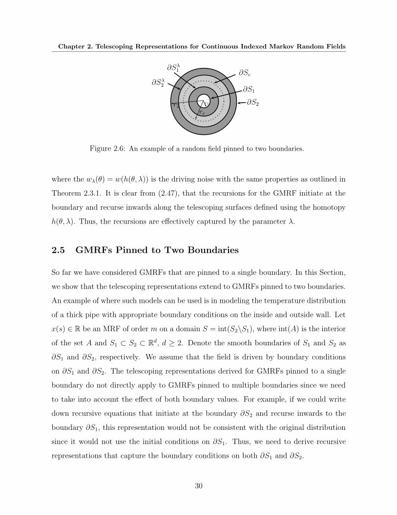
2.6 An example of a random field pinned to two boundaries. . . . . . . . . . . . . 30
xi
LIST OF FIGURES
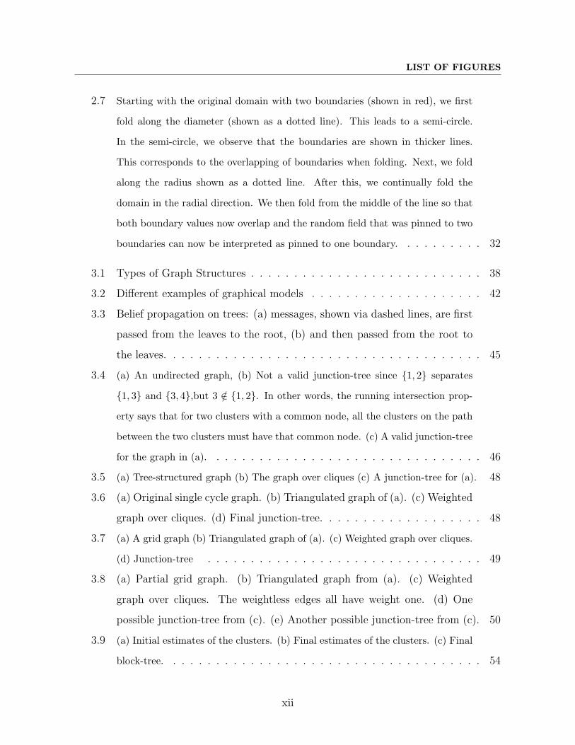
2.7 Starting with the original domain with two boundaries (shown in red), we first
fold along the diameter (shown as a dotted line). This leads to a semi-circle.
In the semi-circle, we observe that the boundaries are shown in thicker lines.
This corresponds to the overlapping of boundaries when folding. Next, we fold
along the radius shown as a dotted line. After this, we continually fold the
domain in the radial direction. We then fold from the middle of the line so that
both boundary values now overlap and the random field that was pinned to two
boundaries can now be interpreted as pinned to one boundary. . . . . . . . . . 32
3.1 Types of Graph Structures . . . . . . . . . . . . . . . . . . . . . . . . . . . 38
3.2 Different examples of graphical models . . . . . . . . . . . . . . . . . . . . 42
3.3 Belief propagation on trees: (a) messages, shown via dashed lines, are first
passed from the leaves to the root, (b) and then passed from the root to
the leaves. . . . . . . . . . . . . . . . . . . . . . . . . . . . . . . . . . . . . 45
3.4 (a) An undirected graph, (b) Not a valid junction-tree since 1, 2 separates
1, 3 and 3, 4,but 3 /∈ 1, 2. In other words, the running intersection prop-
erty says that for two clusters with a common node, all the clusters on the path
between the two clusters must have that common node. (c) A valid junction-tree
for the graph in (a). . . . . . . . . . . . . . . . . . . . . . . . . . . . . . . . 46
3.5 (a) Tree-structured graph (b) The graph over cliques (c) A junction-tree for (a). 48
3.6 (a) Original single cycle graph. (b) Triangulated graph of (a). (c) Weighted
graph over cliques. (d) Final junction-tree. . . . . . . . . . . . . . . . . . . 48
3.7 (a) A grid graph (b) Triangulated graph of (a). (c) Weighted graph over cliques.
(d) Junction-tree . . . . . . . . . . . . . . . . . . . . . . . . . . . . . . . . 49
3.8 (a) Partial grid graph. (b) Triangulated graph from (a). (c) Weighted
graph over cliques. The weightless edges all have weight one. (d) One
possible junction-tree from (c). (e) Another possible junction-tree from (c). 50
3.9 (a) Initial estimates of the clusters. (b) Final estimates of the clusters. (c) Final
block-tree. . . . . . . . . . . . . . . . . . . . . . . . . . . . . . . . . . . . . 54
xii
LIST OF FIGURES
3.10 (a) Original estimates of the clusters in the grid graph when running the forward
pass of Algorithm 2 (b) The final clusters after running the backwards pass of
Algorithm 2 (c) Final block-tree. . . . . . . . . . . . . . . . . . . . . . . . . 55
3.11 (a) Original estimates of the clusters in the partial grid when running the forward
pass of Algorithm 2 (b) The final clusters after running the backwards pass of
Algorithm 2 (c) Final block-tree. . . . . . . . . . . . . . . . . . . . . . . . . 55
3.12 (a) Junction-tree for the block-tree in Fig. 3.10(c) (b) Junction-tree for the block-
tree in Fig. 3.11(c) . . . . . . . . . . . . . . . . . . . . . . . . . . . . . . . . 57
3.13 The relationship between the set of all block-trees and the set of all junction-trees
for a given graph G. . . . . . . . . . . . . . . . . . . . . . . . . . . . . . . . 58
3.14 (a) Original estimates of the clusters in the partial grid using V1 = 7, 4 as the
root cluster (b) Splitting of clusters (c) Final block-tree. . . . . . . . . . . . . 61
3.15 Plot showing the performance of three different greedy heuristics for finding
optimal block-trees. . . . . . . . . . . . . . . . . . . . . . . . . . . . . . . . 62
3.16 Complexity of inference . . . . . . . . . . . . . . . . . . . . . . . . . . . . . 64
3.17 Algorithm to choose between a block-tree and a junction-tree for inference over
graphical models. . . . . . . . . . . . . . . . . . . . . . . . . . . . . . . . . . 66
4.1 A framework for generalizing algorithms on graphical models. . . . . . . . 72
4.2 Example illustrating how to generalize algorithms on graphical models. . . 73
4.3 Explaining Step 6 in the block-graph construction algorithm. Given the block-
graph in (a), if we merge nodes 2 and 3, we get the block-graph in (b). If we
merge nodes 3 and 4, we get the block-graph in (c). Notice that the block-graph
in (c) has just one loop. . . . . . . . . . . . . . . . . . . . . . . . . . . . . . 76
4.4 Comparison of convergence and accuracy of using LBP on graphs vs. using LBP
on block-graphs for a 7×7 grid graph. Results are over 500 runs. The iterations
and accuracy results are when all the algorithms converge. . . . . . . . . . . . 78
xiii

LIST OF FIGURES
4.5 Comparison of convergence and accuracy of using LBP on graphs vs. using LBP
on block-graphs for a 8×8 grid graph. Results are over 200 runs. The iterations
and accuracy results are when all the algorithms converge. . . . . . . . . . . . 78
4.6 Comparison of convergence and accuracy of using LBP on graphs vs. using LBP
on block-graphs for a 30 × 30 grid graph. Results are over 100 runs. Since
finding the true node potentials is computatinally intractable, we use a higher
order block-graph to estimate the ground truth. . . . . . . . . . . . . . . . . . 80
5.1 An example of the tree-structures we derive in this thesis. For MRFs over
continuous indices, we derive tree representations over hypersurfaces. For MRFs
over graphs, we derive tree representations over a disjoint collection of clusters
over nodes. . . . . . . . . . . . . . . . . . . . . . . . . . . . . . . . . . . . . 84
xiv

Chapter 1
Introduction
1.1 Motivation
Recent advances in technology, including data storage and sensing, have led to massive
data collection in nearly all fields of study. A central challenge in analyzing these large
data sets is to find parsimonious stochastic models to describe the data and further de-
rive efficient algorithms that use these stochastic models to make decisions on future
observations. Such algorithms can have a major impact on a variety of different prob-
lems in various domains. For example, in weather monitoring, it is of interest to detect
catastrophic events like fire, hurricane, and floods given noisy measurements from sensor
networks [14]. In analyzing satellite images or hyperspectral images, it is of interest to
detect the presence or absence of certain objects and also to denoise images cluttered with
noise [30], [85]. In computational biology, given stochastic models for gene expressions,
it is of interest to design algorithms for detecting the presence or absence of a particular
diseases [27], [65]. Another example in this domain is to predict protein structures given
a particular protein sequence [113], [118]. In communication systems, it is of interest to
derive efficient and accurate algorithms for decoding a noisy message [28].
A common feature of the problems listed above is that we are given a global probabil-
ity distribution over a collection of random variables, using which we want to make local
estimates about the state of each random variable. Even when the global probability dis-
1
Chapter 1. Introduction
tribution encodes local dependencies among random variables, for example, intensities of
pixels only depending on its neighboring pixel values or genes correlated with similar type
of genes, the problem of manipulating such probability distributions for local decisions is
computationally challenging.
The central theme in this thesis is to find structures in global probability distributions
that can enable efficient algorithms for processing data. Motivated by algorithms that
are efficient on tree-structured like distributions, like Kalman filters [39], [40], recursive
smoothers [37], and belief propagation [69], we focus on finding tree-structured like repre-
sentations for a collection of random variables modeled as a Markov random field (MRFs).
In particular, we consider two kinds of MRFs: (i) MRFs indexed over continuous indices,
and (ii) MRFs indexed over graphs. For both of these kinds of MRFs, we show that
tree-structures can be found, which enable the extension of current known algorithms to
more complex probability distributions.
1.2 Markov Random Fields Over Continous Indices
1.2.1 Literature Review
When modeling random processes, a collection of random variables indexed over some
continuous interval of the real line, the Markov property leads to recursive representations.
Such representations lend themselves to efficient algorithms, an example of which is the
celebrated Kalman filter. Informally, the Markov property for random processes says that
given knowledge of the past and present, the future values only depend on the present
values. This conditional relationship between past, present, and future is also termed a
causal relationship. Markov random processes have been studied extensively and have
been used successfully as mathematical models for time-varying random signals.
In 1931, Schrodinger [81] considered the problem of studying the dynamics of a random
process conditioned on both past and future values. A general study of such processes was
conducted in 1932 by Bernstein [9], where he introduced the notion of a reciprocal process.
Informally, a random process defined on an interval [0, T ] is reciprocal if given any interval
2
1.2. Markov Random Fields Over Continous Indices
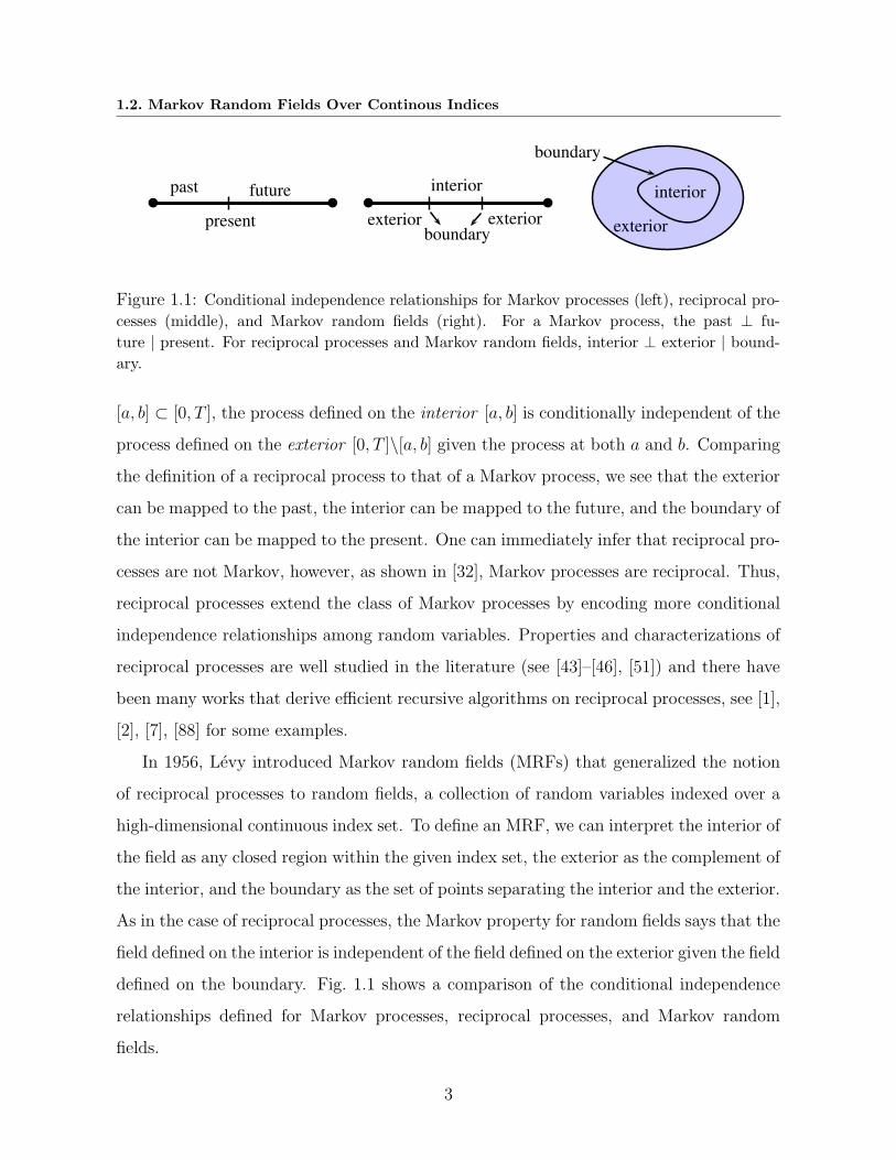
futurepast
present
interior
exteriorexteriorboundary
interior
exterior
boundary
Figure 1.1: Conditional independence relationships for Markov processes (left), reciprocal pro-
cesses (middle), and Markov random fields (right). For a Markov process, the past ⊥ fu-
ture | present. For reciprocal processes and Markov random fields, interior ⊥ exterior | bound-
ary.
[a, b] ⊂ [0, T ], the process defined on the interior [a, b] is conditionally independent of the
process defined on the exterior [0, T ]\[a, b] given the process at both a and b. Comparing
the definition of a reciprocal process to that of a Markov process, we see that the exterior
can be mapped to the past, the interior can be mapped to the future, and the boundary of
the interior can be mapped to the present. One can immediately infer that reciprocal pro-
cesses are not Markov, however, as shown in [32], Markov processes are reciprocal. Thus,
reciprocal processes extend the class of Markov processes by encoding more conditional
independence relationships among random variables. Properties and characterizations of
reciprocal processes are well studied in the literature (see [43]–[46], [51]) and there have
been many works that derive efficient recursive algorithms on reciprocal processes, see [1],
[2], [7], [88] for some examples.
In 1956, Levy introduced Markov random fields (MRFs) that generalized the notion
of reciprocal processes to random fields, a collection of random variables indexed over a
high-dimensional continuous index set. To define an MRF, we can interpret the interior of
the field as any closed region within the given index set, the exterior as the complement of
the interior, and the boundary as the set of points separating the interior and the exterior.
As in the case of reciprocal processes, the Markov property for random fields says that the
field defined on the interior is independent of the field defined on the exterior given the field
defined on the boundary. Fig. 1.1 shows a comparison of the conditional independence
relationships defined for Markov processes, reciprocal processes, and Markov random
fields.
3

Chapter 1. Introduction
(a) (b) (c) (d)
Figure 1.2: Examples of hypersurfaces on which we derive recursive representations. In (a),(b),
and (c) we have have hypersurfaces for a field defined on a dics. In (d), we have surfaces defined
on an arbitrary region.
Following the introduction of MRFs by Levy, several authors have studied various
properties and characterizations of MRFs, see [38], [58], [73] for some examples. Further,
MRFs have been used to study the black body radiation problem [59], to study underwater
ambient noise in the ocean [13], and to study temperature distributions in the atmosphere
[36]. However, unlike Markov and reciprocal processes, there exists no general theory for
deriving recursive algorithms on MRFs. Attempts to enable efficient processing of random
fields have been considered in the past; however, all past work either assumes some kind
of temporal behavior in the spatial signal [67], [105], [106], [108] or assumes a particular
structure on the MRF [84].
1.2.2 Summary of Contributions
In Chapter 2, we introduce a framework for deriving algorithms for recursive processing of
Markov random fields (MRFs). We define the notion of a state for MRFs that collect the
values of the field on any smooth hypersurface separating the continuous domain into two
non-intersecting regions. We use this notion of state and an appropriate collection of states
spanning the MRF domain to derive a telescoping representation for MRFs such that the
representations initiate at the boundary of the MRF and recurse on the hypersurfaces in
a telescoping manner. Thus, the hypersurfaces form a tree-structured like representation
for the MRF. For Gaussian MRFs, we show that the telescoping representations can be
captured using a linear stochastic differential equation driven by Brownian motion. Using
the telescoping representation, we derive recursive estimators that extend the Kalman-
4

1.3. Markov Random Fields Over Graphs
2 3
5
4
1
Graphical modelon a block-tree
2
3
1
5
4
Markov chain Markov tree
2
3
1
5
4
General undirectedgraphical model
2
3
1
5
4
Figure 1.3: Examples of various graphical models and a graphical model defined on a block-tree.
Bucy filter and other standard recursive smoothers to random fields.
Using the notion of homotopy, we show that an MRF can admit multiple different
telescoping representations. For example, in Fig. 1.2, we show various collections of
hypersurfaces for an MRF defined on a disc and an MRF defined on an arbitrary con-
tinuous region. For each collection of hypersurfaces, we can define a telescoping repre-
sentation. Moreover, our telescoping representations extend to arbitrary domains with
smooth boundaries indexed over Rd, for d ≥ 2, and even to domains that are pinned to
two boundaries, an example of which is the temperature distribution of a thick cylinder
with boundary conditions on the inside and outside walls.
1.3 Markov Random Fields Over Graphs
1.3.1 Literature Review
Markov random fields over graphs, also known as graphical models, have been studied
extensively in the literature [48]. The nodes in a graph correspond to random variables
(or random vectors) and the edges in the graph capture various conditional independence
relationships among the random variables. One of the most common graphical models is
the discrete-time Markov process, also known as a Markov chain, which is represented by
a chain-structured graph. A generalization of the Markov chain is a Markov tree, defined
on a tree-structured graph. See the first three graphs in Fig 1.3 for some examples.
It is well known that various algorithms over graphical models are efficient for tree-
structured graphs. For example, given the joint probability distribution of a random
5
Chapter 1. Introduction
vector modeled as a graphical model, it is of interest in various applications to find
the marginal distribution of each random variable. This problem is often referred to as
inference. As an example, given a set of noisy observations y = ys of a random vector
x = xs, we want to estimate or infer each xs given the observations y. To do this, we
need to marginalize the distribution p(x|y). Inference in tree-structured graphical models
can be achieved exactly using the belief propagation (BP) algorithm of Pearl [69], which
works by exchanging messages between nodes connected via edges.
For graphical models with loops or cycles, see Fig. 1.3 for an example, performing
exact inference requires the construction of a junction-tree [77]. A junction-tree is a tree-
structured graph formed by clustering nodes in the original graph in such a way that the
clusters have overlapping nodes. A message passing algorithm over the junction-tree can
be derived so that we get exact inference algorithms for graphical models with cycles [49],
[82]. However, there are two main drawbacks in using junction trees for inference. Firstly,
constructing junction-trees has a worst case complexity that is quadratic in the number
of nodes in the graph. Thus, using junction-trees for inference may not be desirable for
applications involving time-varying graphical models. Secondly, when the junction-trees
have large clusters, the complexity of inference will be large. This makes the junction-tree
approach to inference computationally intractable. This has motivated many works that
derive efficient approximate inference algorithms. We refer to [96] for a review of such
algorithms.
1.3.2 Summary of Contributions
We propose an alternative framework for finding tree-structures in graphs. Instead of
forming a tree on a set of overlapping clusters, we propose to use a set of disjoint clusters.
This leads us to the definition of a block-tree, which is a tree-structured graph over clusters
that are disjoint. An example of a block-tree is shown in Fig. 1.3. We show that block-
trees can be constructed efficiently with complexity linear in the number of edges in the
graph. This naturally makes constructing block-trees faster than constructing junction-
trees. Another advantage of block-trees is that the belief propagation algorithm for trees
6
1.4. Thesis Summary and Organization
easily generalizes to block-trees, leading to algorithms for inference over graphical models
with cycles.
Although block-trees are useful for finding tree-structures in graphical models, as in the
case of junction-trees, using block-trees for inference can be computationally intractable
for situations when the size of clusters is too large. In Chapter 4, we use block-trees
to propose a framework for generalizing various algorithms over graphical models. By
splitting large clusters in a block-tree in a structured manner, we form a graph (not a tree)
over the clusters. Our framework for generalizing algorithms over graphical models uses
the block-graph for computation rather than the original graph. We use this framework
to derive efficient approximate inference algorithms.
1.4 Thesis Summary and Organization
The central theme in this thesis is to find tree-structured like representations for a collec-
tion of random variables modeled as a Markov random field (MRF). Examples of random
signals modeled as MRFs include the steady state temperature distribution in a material,
images, gene expressions, among others.
In Chapter 2, we study MRFs over continuous indices. For such MRFs, we show
that a tree like representation can be derived over a collection of hypersurfaces within
the continuous index set. See Fig. 1.2 for examples of such hypersurfaces. Using this
representation, we derive extensions of the Kalman filter and the Rauch-Tung-Striebel
smoother to Gaussian MRFs indexed over continuous indices.
In Chapter 3, we study MRFs over graphs. We show that by appropriately clustering
nodes in the original graph, we get a tree-structured like representation for such MRFs.
We call the tree-structured graph over the clusters a block-tree. See Fig. 1.2 for an
example of a block-tree. We outline a linear time complexity algorithm for constructing
block-trees. For the problem of inference (computing marginal distributions), we show
the merits of using block-trees over junction-trees, another framework for finding tree-
structures in graphs using a set of overlapping clusters.
7

Chapter 1. Introduction
In Chapter 4, we propose a framework for generalizing various algorithms over graph-
ical models. The key idea is to map the original graph into a block-graph, defined as
graph over disjoint clusters of nodes. We propose an efficient algorithm for constructing
block-graphs by modifying our algorithm for constructing block-trees. As a particular ex-
ample, we demonstrate the use of block-graphs in improving the accuracy of loopy belief
propagation for inference in graphical models.
Chapter 5 concludes this thesis and discusses suggestions for future research.
1.5 Bibliographical Notes
Parts of the material presented in this thesis have been published as conference and journal
papers.
• The material in Chapter 2 has been published in the IEEE Transactions on Informa-
tion Theory [92] in March 2011 and presented in part at the 2010 IEEE Conference
on Decision and Control [89]. The results were motivated by earlier work done on
studying reciprocal processes in [87] and [88].
• Preliminary results from Chapter 3 were presented at the 2010 IEEE International
Conference Acoustics, Speech, and Signal Processing [90].
8

Chapter 2
Telescoping Representations for
Continuous Indexed Markov
Random Fields
2.1 Introduction
In this Chapter, we derive recursive representations for spatially distributed signals, such
as temperature in materials, concentration of components in process control, intensity of
images, density of a gas in a room, stress level of different locations in a structure, or
pollutant concentration in a lake [72], [80], [86]. These signals are often modeled using
random fields, which are random signals indexed over Rd or Z
d, for d ≥ 2. Our focus in
this Chapter will be on random signals indexed over Rd and subsequent Chapters in this
thesis will consider random signals indexed over discrete indices.
For random processes, that are indexed over R, recursive algorithms are recovered
by assuming causality. In particular, for Markov random processes, the future states
depend only on the present state given both the past and present states. When modeling
spatial distributions by random fields, it is more appropriate to assume noncausality as
opposed to causality. This leads to noncausal Markov random fields (MRFs): the field
inside a domain is independent of the field outside the domain given the field on (or
9

Chapter 2. Telescoping Representations for Continuous Indexed Markov Random Fields
(c)(b)(a) (d)
Figure 2.1: Different kinds of telescoping recursions for an MRF defined on a disc.
near) the domain boundary [54]. The need for recursive algorithms for noncausal MRFs
arises to reduce the increased computational complexity due to the noncausality and the
multidimensionality of the index set. The assumption of noncausality presents problems
in developing recursive algorithms, such as the Kalman-Bucy filter for noncausal MRFs.
2.1.1 Summary of Contributions
Telescoping Recursive Representations
We present telescoping recursive representations for noncausal Gaussian Markov random
fields (GMRFs) defined on a closed continuous index set in Rd, d ≥ 2. The telescoping
recursions initiate at the boundary of the field and recurse inwards. For example, in
Fig. 2.1(a), for an MRF defined on a unit disc, we derive telescoping representations
that recurse radially inwards to the center of the field. For the same field, we derive an
equivalent representation where the telescoping surfaces are not necessarily symmetric
about the center of the disc, see Fig. 2.1(b). The telescoping surfaces, under appropriate
conditions, can be arbitrary as shown in Fig. 2.1(c). Finally, for GMRFs pinned to two
boundaries, the telescoping representation initiates from both the boundaries and recurses
towards a hypersurface within the field as shown in Fig. 2.1(d).
We parametrize the field using two parameters: λ ∈ [0, 1] and θ ∈ Θ ⊂ Rd−1. The
parameter λ indicates the position of the telescoping surface and the set Θ parameterizes
the boundary of the index set. For example, for the unit disc with recursions as in
Fig. 2.1(a), the telescoping surfaces are circles, and we can use polar coordinates to
parameterize the field: radius λ and angle θ ∈ Θ = [−π, π]. The telescoping surfaces are
10
2.1. Introduction
represented using a homotopy from the boundary of the field to a point within the index
set (which is not on the boundary). The net effort for d = 2 is to represent the field by a
recursion in λ, i.e., a single parameter (or dimension) rather than multiple dimensions.
The key idea in deriving the telescoping representation is to establish a notion of
“time” for Markov random fields. We show that the parameter λ, which corresponds to
the telescoping surface, acts as time. In our telescoping representation, we define the
state to be the field values at the telescoping surfaces. For Gaussian MRFs (GMRFs),
the telescoping recursive representation results in a linear stochastic differential equation
in the parameter λ and is driven by Brownian motion. For a certain class of homogeneous
isotropic GMRFs over R2, for which the covariance is a function of the Euclidean distance
between points, we show that the driving noise is 2-D white Gaussian noise. For the
Whittle field [102] defined over a unit disc, we show that the driving noise is zero and the
field is uniquely determined using the boundary conditions.
Recursive Estimation of MRFs
Using the telescoping recursive representation, we promptly recover recursive algorithms
well known for Markov random processes. As an example, for GMRFs, we derive exten-
sions of the Kalman-Bucy filter [40] and the Rauch-Tung-Striebel (RTS) smoother [75].
For the Kalman-Bucy filter, we sweep the observations over the telescoping surfaces start-
ing at the boundary and recursing inwards. For the smoother, we sweep the observations
starting from the inside and recursing outwards. Although we use the RTS smoother,
other known smoothing algorithms can be used as well, see [6], [26], [37].
2.1.2 Related Work
Markov random fields (MRFs) indexed over continuous indices have been studied exten-
sively in the literature, starting from work by Levy [54] to subsequent works by McK-
ean [58], Wong [103], Pitt [73], Kallianpur and Mandrekar [38], Rozanov [79], Wong and
Zakai [109], and Moura and Goswami [63]. These works have mainly focused on theo-
retical foundations of MRFs, where the authors have characterized various properties of
11
Chapter 2. Telescoping Representations for Continuous Indexed Markov Random Fields
MRFs. For MRFs indexed over a one-dimensional domain, called reciprocal processes [9],
[32], there has been a lot of work on deriving recursive representations and subsequently
recursive estimators. For example, in [1], [2], [7], the authors derived recursive estimators
for a class for reciprocal processes characterized by a solution to a stochastic differential
equation with mixed boundary conditions. In [88], the authors derived recursive represen-
tations and recursive estimators for reciprocal processes characterized by solutions to a
second order stochastic differential equation driven by correlated noise, see [45]. However,
these representations do not generalize to MRFs indexed over high dimensional continu-
ous domains. Further, algorithms proposed for estimation over discrete indexed MRFs,
see [53], [62], [69], [110], do not generalize to continuous indexed MRFs.
Wong and coauthors have studied the problem of recursive estimation of random fields,
see [67], [104]–[106], [108]. However, the random fields considered by Wong do not capture
spatial variability of noncausal random fields and are causal in some sense. For noncausal
isotropic Gaussian MRFs (GMRFs) over R2, the authors in [84] derived recursive repre-
sentations, and subsequently recursive estimators, by transforming the 2-D problem into
a countably infinite number of 1-D problems. This transformation was possible because of
the isotropy assumption since isotropic fields over R2, when expanded in a Fourier series
in terms of the polar coordinate angle, the Fourier coefficient processes of different orders
are uncorrelated [84]. In this way, the authors derived recursive representations for the
Fourier coefficient process. The recursions in [84] are with respect to the radius when the
field is represented in polar coordinate form. The algorithm is an approximate recursive
estimation algorithm since it requires solving a set of countably infinite number of 1-D
estimation problems [84].
2.1.3 Chapter Organization
The organization of the Chapter is as follows. Section 2.2 reviews the theory of GMRFs.
Section 2.3 introduces the telescoping representation for GMRFs indexed on a unit disc.
Section 2.4 generalizes the telescoping representations to arbitrary domains. Section 2.5
extends the telescoping representations to GMRFs pinned to two boundaries. Section 2.6
12

2.2. Gauss-Markov Random Fields
derives recursive estimation algorithms using the telescoping representation. Section 2.7
summarizes the Chapter.
2.2 Gauss-Markov Random Fields
For a random process x(s), s ∈ R, the notion of Markovianity corresponds to the as-
sumption that the past x(s) : s < t, and the future x(s) : s > t are conditionally
independent given the present x(s). Higher order Markov processes can be considered
when the past is independent of the future given the present and information near the
present. The extension of this definition to random fields, i.e., a random process indexed
over Rd for d ≥ 2, was introduced in [54]. Specifically, a random field x(s), s ∈ S ⊂ R
d, is
Markov if for any smooth surface ∂G separating S into complementary domains, the field
inside is independent of the field outside conditioned on the field on (and near) ∂G. To
capture this definition in a mathematically precise way, we use the notation introduced
in [58]. On the probability space (Ω,F ,P), let1 x(s) ∈ R be a zero mean random field
for s ∈ S ⊂ Rd, where d ≥ 2 and let ∂S ⊂ S be the smooth boundary of S. For any set
A ⊂ S, denote x(A) as
x(A) = x(s) : s ∈ A . (2.1)
Let G− ⊂ S be an open set with smooth boundary ∂G and let G+ be the complement of
G− ∪ ∂G in S. Together, G− and G+ are called complementary sets. Fig. 2.2(a) shows
an example of the sets G−, G+, and ∂G on a domain S ⊂ R2. For ε > 0, define the set
of points from the boundary ∂G at a distance less than ε
∂Gε = s ∈ S : d(s, ∂G) < ε , (2.2)
1For ease in notation, we assume x(s) ∈ R, however our results remain valid for x(s) ∈ Rn, when
n ≥ 2.
13

Chapter 2. Telescoping Representations for Continuous Indexed Markov Random Fields
G−G+
∂S∂G
∂G
G− G+
(a) (b)
Figure 2.2: (a) An example of complementary sets on a random field defined on S with boundary
∂S. (b) Corresponding notion of complementary sets for a random process.
where d(t, ∂G) is the distance of a point s ∈ S to the set of points ∂G. On G± and ∂G,
define the sets
Σx(G±) = σ(x(G±)) (2.3)
Σx(∂G) =⋂
ε>0
σ(x(∂Gε)) , (2.4)
where σ(A) stands for the σ-algebra generated by the set A. If x(s) is a Markov ran-
dom field, the conditional expectation of x(s), s /∈ G−, given Σx(G−) is the conditional
expectation of x(s) given Σx(∂G), i.e., [58], [73]
E[x(s)|Σx(G−)] = E[x(s)|Σx(∂G)] , s /∈ G− . (2.5)
Equation (2.5) also holds for Markov random processes for complementary sets defined as
in Fig. 2.2(b). In the context of Markov processes, the set G− in Fig. 2.2(b) is called the
“past”, G+ is called the “future”, and ∂G is called the “present”. The equivalent notions
of past, present, and future for random fields is clear from the definition of G−, G+, and
∂G in Fig. 2.2(a).
To derive linear stochastic differential equations of MRFs, we assume x(s) is zero
mean Gaussian, giving us a Gauss-Markov random field (GMRF), so the conditional
expectation in (2.5) becomes a linear projection. Following [73], the key assumptions we
make throughout the paper are as follows.
14
2.2. Gauss-Markov Random Fields
A1. We assume the index set S ⊂ Rd is a connected2 open set with smooth boundary
∂S.
A2. The zero mean GMRF x(s) ∈ L2(Ω,F ,P), which means that x(s) has finite energy.
A3. The covariance of x(s) is R(t, s), where t, s ∈ S ⊂ Rd. The function space of R(t, s)
is associated with the uniformly strongly elliptic inner product
< u, v > =⟨Dαu, aα,βD
βv⟩
T(2.6)
=∑
|α|≤m,|β|≤m
∫
T
Dαu(s)aα,β(s)Dβv(s)ds , (2.7)
where aα,β are bounded, continuous, and infinitely differentiable, α = [α1, · · · , αd] is
a multi-index of order |α| = α1+· · ·+αd and the operator Dα is the partial derivative
operator
Dα = Dα1
1 · · ·Dαd
d , (2.8)
where Dαi
i = ∂αi/∂tαi
i for t = [t1, . . . , td].
A4. Since the inner product in (2.7) is uniformly strongly elliptic, it follows as a conse-
quence of A3 that R(t, s) is jointly continuous, and thus x(s) can be modified to have
continuous sample paths. We assume that this modification is done, so the GMRF
x(s) has continuous sample paths.
Under Assumptions A1-A4, we now review results on GMRFs we use in this Chapter.
Weak normal derivatives: Let ∂G be a boundary separating complementary sets G−
and G+. Whenever we refer to normal derivatives, they are to be interpreted in the
following weak sense: For every smooth f(t),
y(s) =∂
∂nx(s)
⇒
∫
∂G
f(s)y(s)dl = limh→0
∂
∂h
∫
∂G
f(s)x(s+ hs)dl , (2.9)
2A set is connected if it can not be divided into disjoint nonempty closed set.
15
Chapter 2. Telescoping Representations for Continuous Indexed Markov Random Fields
where dl is the surface measure on ∂G and s is the unit vector normal to ∂G at the point
s.
GMRFs with order m: Throughout the paper, unless mentioned otherwise, we assume
that the GMRF has order m, which can have multiple different equivalent interpretation:
(i) the GMRF x(s) has m−1 normal derivatives, defined in the weak sense, for each point
s ∈ ∂G for all possible surfaces ∂G, (ii) the σ-algebra Σx(∂G) in (2.4), called the germ σ-
algebra, contains information about m−1 normal derivatives of the field on the boundary
∂G [73], or (iii) there exists a symmetric and positive strongly elliptic differential operator
Lt with order 2m such that [63]
LtR(t, s) = δ(t− s) , (2.10)
where the differential operator has the form,
Ltu(t) =∑
|α|,|β|≤m
(−1)|α|Dα[aα,β(t)Dβ(u(t))] . (2.11)
Prediction: The following theorem, proved in [73], gives us a closed form expression for
the conditional expectation in (2.5).
Theorem 2.2.1 ( [73]). Let x(s), s ∈ S ⊂ Rd, be a zero mean GMRF of order m and
covariance R(t, s). Consider complementary sets G− and G+ with common boundary ∂G.
For s /∈ G−, the conditional expectation of x(s) given Σx(G−) is
E[x(s)|Σx(G−)] =m−1∑
j=0
∫
∂G
bj(s, r)∂j
∂njx(r)dl , (2.12)
where ∂j/∂nj is the normal derivative, defined in (2.9), dl is a surface measure on the
boundary ∂G, and the functions bj(s, r), s /∈ G− and r ∈ ∂G, are smooth.
Proof. A detailed proof of Theorem 2.2.1 can be found in [73], where the result is proved
for the case when s ∈ G+. To include the case when s ∈ ∂G, we use the fact that R(t, s)
16

2.3. Telescoping Representation: GMRFs on a Unit Disc
is jointly continuous (consequence of A3) and the uniform integrability of the Gaussian
measure (see [4]).
Theorem 2.2.1 says that for each point outside G−, the conditional expectation given
all the points in G− depends only the field defined on or near the boundary. This is not
surprising since, as stated before, E[x(s)|Σx(G−)] = E[x(s)|Σx(∂G)], and we mentioned
before that Σx(∂G) has information about the m − 1 normal derivatives of x(s) on the
surface ∂G. Appendix A.1 shows how the smooth functions bj(s, r) can be computed and
outlines an example of the computations in the context of a Gauss-Markov process. In
general, Theorem 2.2.1 extends the notion of a Gauss-Markov process of order m (or an
autoregressive process of order m) to random fields.
A simple consequence of Theorem 2.2.1 is that we get the following characterization
for the covariance of a GMRF of order m.
Theorem 2.2.2. If s ∈ G− and s /∈ G−, the covariance R(t, s) can be written as,
R(s, t) =m−1∑
j=0
∫
∂G
bj(s, r)∂j
∂njR(r, t)dl , (2.13)
where the normal derivative in (2.13) is with respect to the variable r.
Proof. Since x(s)−E[x(s)|Σx(G−)] ⊥ x(s) for s ∈ G−, using (2.12), we can easily establish
(2.13).
Theorem 2.2.2 says that the covariance R(s, t) of a GMRF can be written in terms of
the covariance of the field defined on a boundary dividing s and t. Both Theorems 2.2.1
and 2.2.2 will be used in deriving the telescoping recursive representation.
2.3 Telescoping Representation: GMRFs on a Unit Disc
In this Section, we present the telescoping recursive representation for GMRFs indexed
over a domain S ⊂ R2, which is assumed to be a unit disc centered at the origin. The gen-
eralization to arbitrary domains is presented in Section 2.4. To parametrize the GMRF,
17

Chapter 2. Telescoping Representations for Continuous Indexed Markov Random Fields
x(∂S)
x(∂Sλ2)
x(∂Sλ1)
xλ1(θ)
Figure 2.3: A random field defined on a unit disc. The boundary of the field, i.e., the field
values defined on the circle with radius 1 is denoted by x(∂S). The field values at a distance
of 1 − λ from the center of the field are given by x(∂Sλ). Each point is characterized in polar
coordinates as xλ(θ), where 1− λ is the distance to the center and θ denotes the angle.
say x(s) for s ∈ S, we use polar coordinates such that xλ(θ) is defined to be the point
xλ(θ) = x((1− λ) cos θ, (1− λ) sin θ) , (2.14)
where (λ, θ) ∈ [0, 1]× [−π, π]. Thus, x0(θ) : θ ∈ [−π, π] corresponds to the field defined
on the boundary of the unit disc, denoted as ∂S. Let ∂Sλ denote the set of points in S at
a distance 1− λ from the center of the field. We call ∂Sλ a telescoping surface since the
telescoping representations we derive recurse these surfaces. The notations introduced so
far are shown in Fig. 2.3.
2.3.1 Main Theorem
Before deriving our main theorem regarding the telescoping representation, we first define
some notation. Let x(s) ∈ R be a zero mean GMRF defined on a unit disc S ⊂ R2
parametrized as xλ(θ), defined in (2.14). Let Θ = [−π, π] and denote the covariance
between xλ1(θ1) and xλ2
(θ2) by Rλ1,λ2(θ1, θ2) such that
Rλ1,λ2(θ1, θ2) = E[xλ1
(θ1)xλ2(θ2)] . (2.15)
18
2.3. Telescoping Representation: GMRFs on a Unit Disc
Define Cλ(θ1, θ2) and Bλ(θ) as
Cλ(θ1, θ2) = limµ→λ−
∂
∂µRµ,λ(θ1, θ2)− lim
µ→λ+
∂
∂µRµ,λ(θ1, θ2) (2.16)
Bλ(θ) =
√Cλ(θ, θ) Cλ(θ, θ) 6= 0
K Cλ(θ, θ) = 0, (2.17)
where K is any non-zero constant. We will see in (A.31) that Cλ(θ, θ) is the variance of
a random variable and hence it is non-negative. Define Fθ as the integral transform
Fθ[xλ(θ)] =m−1∑
j=0
∫
Θ
limµ→λ+
∂
∂µbj((µ, θ), (λ, α))
∂j
∂njxλ(α)dα , (2.18)
where bj((µ, θ), (λ, α)) is defined in (2.12) and the index (µ, θ) in polar coordinates cor-
responds to the point ((1 − µ) cos θ, (1 − µ) sin θ) in Cartesian coordinates. We see that
Fθ[xλ(θ)] operates on the surface ∂Sλ such that it is a linear combination of all normal
derivatives of xλ(θ) up to order m− 1. The normal derivative in (2.18) is interpreted in
the weak sense as defined in (2.9). We now state the main theorem of the paper.
Theorem 2.3.1 (Telescoping Recursive Representation). For the GMRF parametrized
as xλ(θ), defined in (2.14), we have the following stochastic differential equation
dxλ(θ) = Fθ[xλ(θ)]dλ+Bλ(θ)dwλ(θ) , (2.19)
where dxλ(θ) = xλ+dλ(θ)− xλ(θ) for dλ small, Fθ is defined in (2.18), Bλ(θ) is defined in
(2.17), and wλ(θ) has the following properties:
i) The driving noise wλ(θ) is zero mean Gaussian, almost surely continuous in λ, and
independent of x(∂S) (the field on the boundary).
ii) For all θ ∈ Θ, w0(θ) = 0.
iii) For 0 ≤ λ1 ≤ λ′1 ≤ λ2 ≤ λ′2 and θ1, θ2 ∈ Θ, wλ′1(θ1)− wλ1
(θ1) and wλ′2(θ2)− wλ2
(θ2)
are independent random variables.
19

Chapter 2. Telescoping Representations for Continuous Indexed Markov Random Fields
iv) For θ ∈ Θ, we have
E[wλ(θ1)wλ(θ2)] =
∫ λ
0
Cu(θ1, θ2)
Bu(θ1)Bu(θ2)du . (2.20)
v) Assuming the set u ∈ [0, 1] : Cu(θ, θ) = 0 has measure zero for each θ ∈ Θ, for
λ1 > λ2 and θ1, θ2 ∈ Θ, the random variable wλ1(θ1)−wλ2
(θ2) is Gaussian with mean
zero and covariance
E[(wλ1
(θ1)− wλ2(θ2))
2] = λ1 + λ2 − 2
∫ λ2
0
Cu(θ1, θ2)
Bu(θ1)Bu(θ2)du . (2.21)
Proof. See Appendix A.
Theorem 2.3.1 says that xλ+dλ(θ), where dλ is small, can be computed using the ran-
dom field defined on the telescoping surface ∂Sλ and some random noise. The dependence
on the telescoping surface follows from Theorem 2.2.1. The main contribution in Theo-
rem 2.3.1 is to explicitly compute properties of the driving noise wλ(θ). We now discuss
the telescoping representation and highlight its various properties.
Driving noise wλ(θ): The properties of the driving noise wλ(θ) in (2.19) lead to the
following theorem.
Theorem 2.3.2 (Driving noise wλ(θ)). For the collection of random variables
wλ(θ) : (λ, θ) ∈ [0, 1]×Θ
defined in (2.19), for each fixed θ ∈ Θ, wλ(θ) is a standard Brownian motion when the
set u ∈ [0, 1] : Cu(θ, θ) = 0 has measure zero for each θ ∈ Θ.
Proof. For fixed θ ∈ Θ, to show wλ(θ) is Brownian motion, we need to establish the
following: (i) wλ(θ) is continuous in λ, (ii) w0(θ) = 0 for all θ ∈ Θ, (iii) wλ(θ) has inde-
pendent increments, i.e., for 0 ≤ λ1 ≤ λ′1 ≤ λ2 ≤ λ′2, wλ′1(θ)−wλ1
(θ) and wλ′2(θ)−wλ2
(θ)
are independent random variables, and (iv) for λ1 > λ2, wλ1(θ)−wλ2
(θ) ∼ N (0, λ1−λ2).
20

2.3. Telescoping Representation: GMRFs on a Unit Disc
The first three points follow from Theorem 2.3.1. To show the last point, let θ1 = θ2 in
(2.21) and use the computations done in (A.39)-(A.42).
Theorem 2.3.2 says that for each fixed θ, wλ(θ) in (2.19) is Brownian motion. This is
extremely useful since we can use standard Ito calculus to interpret (2.19).
White noise: A useful interpretation of wλ(θ) is in terms of white noise. Define a random
field vλ(θ) such that
wλ(θ) =
∫ λ
0
vγ(θ)dγ . (2.22)
Using Theorem 2.3.1, we can easily establish that vλ(θ) is a generalized process such that
for an appropriate function Ψ(·),
∫ 1
0
Ψ(γ)E[vγ(θ1)vλ(θ2)]dγ = Ψ(λ)Cλ(θ1, θ2)
Bλ(θ1)Bλ(θ2), (2.23)
which is equivalent to the expression
E[vλ1(θ1)vλ2
(θ2)] = δ(λ1 − λ2)Cλ1
(θ1, θ2)
Bλ1(θ1)Bλ2
(θ2). (2.24)
Using the white noise representation, an alternative form of the telescoping representation
is given bydxλ(θ)
dλ= Fθ[xλ(θ)] +Bλ(θ)vλ(θ) . (2.25)
Boundary Conditions: From the form of the integral transform Fθ in (2.18), it is clear
that boundary conditions for the telescoping representation will be given in terms of the
field defined at the boundary and its normal derivatives. A general form for the boundary
conditions can be given as
m−1∑
j=0
∫
Θ
ck,j(θ, α)∂j
∂njx0(α)dα = βk(θ) , θ ∈ Θ , k = 1, . . . ,m , (2.26)
where for each k, βk(θ) is a Gaussian process in θ with mean zero and known covariance.
21
Chapter 2. Telescoping Representations for Continuous Indexed Markov Random Fields
Integral Form: The representation in (2.19) is a symbolic representation for the equation
xλ1(θ) = xλ2
(θ) +
∫ λ1
λ2
Fθ[xµ(θ)]dµ+
∫ λ1
λ2
Bµ(θ)dwµ(θ) , λ1 > λ2 . (2.27)
Since from Theorem 2.3.2, wλ(θ) is Brownian motion for fixed θ, the last integral in (2.27)
is an Wiener integral. Thus, to recursively synthesize the field, we start with boundary
values, given by (2.26), and generate the field values recursively on the telescoping surfaces
∂Sλ for λ ∈ (0, 1].
Comparison to [84]: The telescoping recursive representation differs significantly from
the recursive representation derived in [84]. Firstly, the representation in [84] is only valid
for isotropic GMRFs and does not hold for nonisotropic GMRFs. The telescoping rep-
resentation we derive holds for arbitrary GMRFs. Secondly, the recursive representation
in [84] was derived on the Fourier series coefficients, whereas we derive a representation
directly on the field values.
2.3.2 Homogeneous and Isotropic GMRFs
In this Section, we study homogeneous isotropic random fields over R2 whose covari-
ance only depends on the Euclidean distance between two points. In general, suppose
Rµ,λ(θ1, θ2) is the covariance of a homogeneous isotropic random field over a unit disc such
that the point (µ, θ1) in polar coordinates corresponds to the point ((1 − µ) cos θ, (1 −
µ) sin θ) in Cartesian coordinates. The Euclidean distance between two points (µ, θ1) and
(λ, θ2) is given by
Dµ,λ(θ1, θ2) =[(1− µ)2 + (1− λ)2 − 2(1− µ)(1− λ) cos(θ1 − θ2)
]1/2. (2.28)
If Rµ,λ(θ1, θ2) is the covariance of a homogeneous and isotropic GMRF, we have
Rµ,λ(θ1, θ2) = Υ (Dµ,λ(θ1, θ2)) , (2.29)
22
2.3. Telescoping Representation: GMRFs on a Unit Disc
where Υ(·) : R → R is assumed to be differentiable at all points in R. The next Lemma
computes Cλ(θ1, θ2) for isotropic and homogeneous GMRFs.
Lemma 2.3.1. For an isotropic and homogeneous GMRF with covariance given by (2.29),
Cλ(θ1, θ2), defined in (2.16), is given by
Cλ(θ1, θ2) =
0 θ1 6= θ2
−2Υ′(0) θ1 = θ2
. (2.30)
Proof. For θ1 6= θ2, we have
∂
∂uRµ,λ(θ1, θ2) = −Υ′ (Dµ,λ(θ1, θ2))
(1− µ)− (1− λ) cos(θ1 − θ2)
Dµ,λ(θ1, θ2), (2.31)
where Υ′(·) is the derivative of the function Υ(·). Using (2.16), Cλ(θ1, θ2) = 0 when
θ1 6= θ2.
For θ1 = θ2, Dµ,λ(θ1, θ2) = |µ− λ|, so we have
∂
∂uRµ,λ(θ1, θ2) = −Υ′(|λ− µ|)
λ− µ
|λ− µ|, (2.32)
Using (2.16), Cλ(θ1, θ2) = −2Υ′(0) when θ1 = θ2.
Using Lemma 2.3.1, we have the following theorem regarding the driving noise wλ(θ)
of the telescoping representation of an isotropic and homogeneous GMRF.
Theorem 2.3.3 (Homogeneous isotropic GMRFs). For homogeneous isotropic GMRFs,
with covariance given by (2.29), such that Υ(·) is differentiable at all points in R and
Υ′(0) < 0, the telescoping representation is
dwλ(θ) = Fθxλ(θ) +√−Υ′(0)dwλ(θ) . (2.33)
For each fixed θ, wλ(θ) is Brownian motion in λ and
E[wλ1(θ1)wλ2
(θ2)] = 0 , λ1 6= λ2, θ1 6= θ2 (2.34)
23

Chapter 2. Telescoping Representations for Continuous Indexed Markov Random Fields
E[wλ(θ1)wλ(θ2)] = 0 , θ1 6= θ2 . (2.35)
Proof. Since we assume Υ′(0) < 0, thus Bλ(θ) = Cλ(θ, θ) =√−Υ′(0), which gives us
(2.33). To show (2.34) and (2.35), we simply substitute the value of Cλ(θ1, θ2), given by
(2.30), in (2.20) and use the independent increments property of wλ(θ) given in Theo-
rem 2.3.1.
Example: We now consider an example of a homogeneous and isotropic GMRF where
Υ′(0) = 0 and thus the field is uniquely determined by the boundary conditions. Let
Υ(s), s ∈ [0,∞), be such that
Υ(t) =
∫ ∞
0
b
(1 + b2)2J0(bt)db , (2.36)
where Jn(·) is the Bessel function of the first kind of order n [97]. The derivative of Υ(t)
is given by
Υ′(t) = −
∫ ∞
0
b2
(1 + b2)2J1(bt)db , (2.37)
where we use the fact that J ′0(·) = −J1(·) [97]. Since J1(0) = 0, Υ′(0) = 0 and thus
Bλ(θ) = 0 in the telescoping representation. This means there is no driving noise in the
telescoping representation. The rest of the parameters of the telescoping representation
can be computed using the fact [103]
(∆− 1)2R(t, s) = δ(t− s) , (2.38)
where R(t, s) corresponds to the covariance associated with Υ(·) written in Cartesian
coordinates and ∆ is the Laplacian operator. Since the operator associated with R(t, s)
in (2.38) has order four, it is clear that the GMRF has order two. The field with covariance
satisfying (2.38) is also commonly referred to as the Whittle field [102]. The telescoping
recursive representation will be of the form
dxλ(θ) =
∫ π
−π
limµ→λ+
[∂
∂ub0((µ, θ), (λ, α))xλ(α) +
∂
∂ub1((µ, θ), (λ, α))
∂
∂nxλ(α)
]dα dλ ,
24
2.4. Telescoping Representation: GMRFs on arbitrary domains
where 0 ≤ λ ≤ 1 with appropriate boundary conditions defined on the unit circle.
2.4 Telescoping Representation: GMRFs on arbitrary domains
In the last Section, we presented telescoping recursive representations for random fields
defined on a unit disc. In this Section, we generalize the telescoping representations
to arbitrary domains. Section 2.4.1 shows how to define telescoping surfaces using the
concept of homotopy. Section 2.4.2 shows how to parametrize arbitrary domains using
the homotopy. Section 2.4.3 presents the telescoping representation for GMRFs defined
on arbitrary domains.
2.4.1 Telescoping Surfaces Using Homotopy
Informally, a homotopy is defined as a continuous deformation from one space to another.
Formally, given two continuous functions f and g such that f, g : X → Y , a homotopy
is a continuous function h : X × [0, 1] → Y such that if x ∈ X , h(x, 0) = f(x) and
h(x, 1) = g(x) [64]. An example of the use of homotopy in neural networks is shown
in [16].
In deriving our telescoping representation for GMRFs on a unit disc in Section 2.3, we
saw that the recursions started at the boundary, which was the unit circle, and telescoped
inwards on concentric circles and ultimately converged to the center of the unit disc.
To parametrize these recursions, we can define a homotopy from the unit circle to the
center of the unit disc. In general, for a domain S ⊂ Rd with smooth boundary ∂S,
the telescoping surfaces can be defined using a homotopy, h : ∂S × [0, 1] → c, from the
boundary ∂S to a point c ∈ S such that
P1. h(s, 0) : s ∈ ∂S = ∂S and h(s, 1) : s ∈ ∂S = c.
P2. For 0 < λ ≤ 1, h(s, λ) : s ∈ ∂S ⊂ S is the boundary of the region h(s, µ) : (s, µ) ∈
∂S × (λ, 1).
P3. For λ1 < λ2, h(s, λ1), s ∈ ∂S ⊂ h(s, µ), s ∈ ∂S, 0 ≤ µ ≤ λ2.
25
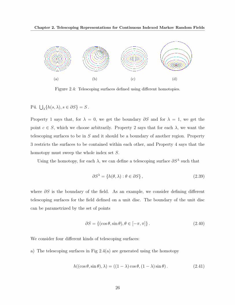
Chapter 2. Telescoping Representations for Continuous Indexed Markov Random Fields
(a) (b) (c) (d)
Figure 2.4: Telescoping surfaces defined using different homotopies.
P4.⋃
λh(s, λ), s ∈ ∂S = S .
Property 1 says that, for λ = 0, we get the boundary ∂S and for λ = 1, we get the
point c ∈ S, which we choose arbitrarily. Property 2 says that for each λ, we want the
telescoping surfaces to be in S and it should be a boundary of another region. Property
3 restricts the surfaces to be contained within each other, and Property 4 says that the
homotopy must sweep the whole index set S.
Using the homotopy, for each λ, we can define a telescoping surface ∂Sλ such that
∂Sλ = h(θ, λ) : θ ∈ ∂S , (2.39)
where ∂S is the boundary of the field. As an example, we consider defining different
telescoping surfaces for the field defined on a unit disc. The boundary of the unit disc
can be parametrized by the set of points
∂S = (cos θ, sin θ), θ ∈ [−π, π] . (2.40)
We consider four different kinds of telescoping surfaces:
a) The telescoping surfaces in Fig 2.4(a) are generated using the homotopy
h((cos θ, sin θ), λ) = ((1− λ) cos θ, (1− λ) sin θ) . (2.41)
26

2.4. Telescoping Representation: GMRFs on arbitrary domains
b) The telescoping surfaces in Fig 2.4(b) can be generated by the homotopy
h((cos θ, sin θ), λ)
= ((1− λ)(cos θ − c1) + c1, (1− λ)(sin θ − c2) + c2) , (2.42)
= ((1− λ) cos θ + c1 − (1− λ)c1, (2.43)
(1− λ) cos θ + c2 − (1− λ)c2) ,
where (c1, c2) is inside the unit disc, i.e., c21 + c22 < 1. For the homotopy in (2.41),
each telescoping surface is centered about the origin, whereas the telescoping surfaces
in (2.43) are centered about the point (c1 − (1− λ)c1, c2 − (1− λ)c2).
c) In Fig 2.4(a)-(b), the telescoping surfaces are circles, however, we can also have other
shapes for the telescoping surface. Fig 2.4(c) shows an example in which the telescoping
surface is an ellipse, which we generate using the homotopy
h((cos θ, sin θ), λ) = (aλ cos θ, bλ sin θ) (2.44)
where aλ and bλ are continuous functions chosen in such a way that P1-P4 are satisfied
for h. In Fig 2.4(c), we choose aλ = λ and bλ = λ2.
d) Another example of a set of telescoping surfaces is shown in Fig 2.4(d). From here,
we notice that two telescoping surfaces may have common points.
Apart from the telescoping surfaces for a unit disc shown in Fig 2.4(a)-(d), we can
define many more telescoping surfaces. The basic idea in obtaining these surfaces, which
is compactly captured by defining a homotopy, is to continuously deform the boundary
of the index set until we converge to a point within the index set. In the next Section,
we provide a characterization of continuous index sets in Rd for which we can easily find
telescoping surfaces by simply scaling and translating the points on the boundary.
27
Chapter 2. Telescoping Representations for Continuous Indexed Markov Random Fields
2.4.2 Generating Similar Telescoping Surfaces
From Section 2.4.1, it is clear that, for a given domain, many different telescoping surfaces
can be obtained by defining different homotopies. In this Section, we identify domains on
which we can easily generate a set of telescoping surfaces, which we call similar telescoping
surfaces.
Definition 1 (Similar Telescoping Surfaces). Two telescoping surfaces are similar if there
exists an affine map between them, i.e., we can map one to another by scaling and translat-
ing of the coordinates. A set of telescoping surfaces are similar if each pair of telescoping
surfaces in the set are similar.
As an example, the set of telescoping surfaces in Fig 2.4(a)-(b) are similar since all the
telescoping surfaces are circles. On the other hand, the telescoping surfaces in Fig 2.4(c)-
(d) are not similar since each telescoping surfaces has a different shape. The following
theorem shows that, for certain index sets, we can always find a set of similar telescoping
surfaces.
Theorem 2.4.1. For a domain T ∈ Rd with boundary ∂S if there exists a point c ∈ S
such that, for all s ∈ S ∪ ∂S and λ ∈ [0, 1], (1 − λ)t + λc ∈ S, we can generate similar
telescoping surfaces using the homotopy
h(θ, λ) = (1− λ)θ + λc , θ ∈ ∂S . (2.45)
Proof. Given the homotopy in (2.45), the telescoping surfaces are given by ∂Sλ = h(θ, λ) :
θ ∈ ∂S. Using (2.45), it is clear that ∂S0 = ∂S and ∂S1 = c. Given the assumption, we
have that ∂Sλ ⊂ S for 0 < λ ≤ 1. Since the distance of each point on ∂Sλ to the point
c is (1− λ)||θ − c||, it is clear that, for λ1 < λ2, ∂Sλ1 ⊂ ∂Sµ : 0 ≤ µ ≤ λ2. This shows
that the homotopy in (2.45) defines a valid telescoping surface. The set of telescoping
surfaces is similar since we are only scaling and translating the boundary ∂S.
Examples of similar telescoping surfaces generated using the homotopy in (2.45) are
shown in Fig 2.5(a) and Fig 2.5(c). Choosing an appropriate c is important to generate
28

2.4. Telescoping Representation: GMRFs on arbitrary domains
(a) (b) (c) (d)
Figure 2.5: Telescoping surfaces defined using different homotopies on arbitrary regions.
similar telescoping surfaces. For example, Fig 2.5(b) shows an example where telescoping
surfaces are generated using (2.45). It is clear that these surfaces do not satisfy the
desired properties of telescoping surfaces. Fig 2.5(d) shows an example of an index set
for which similar telescoping surfaces do not exist since there exists no point c for which
(1− λ)s+ λc ∈ S for all λ ∈ [0, 1] and s ∈ S ∪ ∂S.
2.4.3 Telescoping Representations
We now generalize the telescoping representation to GMRFs defined on arbitrary domains.
Let x(s) be a zero mean GMRF, where s ∈ S ⊂ Rd such that the smooth boundary of
S is ∂S. Define a set of telescoping surfaces ∂Sλ constructed by defining a homotopy
h(θ, λ), where θ ∈ ∂S and λ ∈ [0, 1]. We parametrize the GMRF x(s) as xλ(θ) such that
xλ(θ) = x(h(θ, λ)) . (2.46)
Denote Θ = ∂S and define Cλ(θ1, θ2), Bλ(θ), and Fθ by (2.16), (2.17), and (2.18), re-
spectively. Although the initial definition for these values was for Θ = [−π, π] and xλ(θ)
parametrized in polar coordinates, assume the definitions in (2.16), (2.17), and (2.18) are
in terms of the parameters defined in this Section. The normal derivatives in the defini-
tion of Fθ for a point xλ(θ) will be computed in the direction normal to the telescoping
surface ∂Sλ at the point h(θ, λ). The telescoping representation is given by
dxλ(θ) = Fθ[xλ(θ)]dλ+Bλ(θ)dwλ(θ) (2.47)
29
Chapter 2. Telescoping Representations for Continuous Indexed Markov Random Fields
∂S1
∂S2
∂Sc∂Sλ
1
∂Sλ2
r1
rc
r2
Figure 2.6: An example of a random field pinned to two boundaries.
where the wλ(θ) = w(h(θ, λ)) is the driving noise with the same properties as outlined in
Theorem 2.3.1. It is clear from (2.47), that the recursions for the GMRF initiate at the
boundary and recurse inwards along the telescoping surfaces defined using the homotopy
h(θ, λ). Thus, the recursions are effectively captured by the parameter λ.
2.5 GMRFs Pinned to Two Boundaries
So far we have considered GMRFs that are pinned to a single boundary. In this Section,
we show that the telescoping representations extend to GMRFs pinned to two boundaries.
An example of where such models can be used is in modeling the temperature distribution
of a thick pipe with appropriate boundary conditions on the inside and outside wall. Let
x(s) ∈ R be an MRF of order m on a domain S = int(S2\S1), where int(A) is the interior
of the set A and S1 ⊂ S2 ⊂ Rd, d ≥ 2. Denote the smooth boundaries of S1 and S2 as
∂S1 and ∂S2, respectively. We assume that the field is driven by boundary conditions
on ∂S1 and ∂S2. The telescoping representations derived for GMRFs pinned to a single
boundary do not directly apply to GMRFs pinned to multiple boundaries since we need
to take into account the effect of both boundary values. For example, if we could write
down recursive equations that initiate at the boundary ∂S2 and recurse inwards to the
boundary ∂S1, this representation would not be consistent with the original distribution
since it would not use the initial conditions on ∂S1. Thus, we need to derive recursive
representations that capture the boundary conditions on both ∂S1 and ∂S2.
30

2.5. GMRFs Pinned to Two Boundaries
For notational simplicity, we assume S1 and S2 are discs in R2. The representations
derived can be easily generalized to arbitrary domains using homotopy. We assume S1
(S2) is a disc of radius r1 (r2), where r1 < r2. Consider a disc Sc of radius rc, as shown
in Fig. 2.6, such that r1 < rc < r2 and denote its boundary as ∂Sc. We parametrize the
GMRF using polar coordinates such that
xµ(θ) = x(µ cos θ, µ sin θ), r1 < µ < r2, θ ∈ [0, 2π) . (2.48)
For 0 ≤ λ ≤ 1, let ∂Sλ1 be the boundary of the disc Sλ
1 with radius r1 + λ(rc − r1) and
let ∂Sλ2 be the boundary of the disc Sλ
2 with radius r2 + λ(rc − r2). We see that Sλ1 lies
between S1 and Sc and Sλ2 lies between S2 and Sc. The notations introduced so far are
shown in Fig. 2.6. Define zcλ(θ) ∈ R
2 on ∂Sλ1 and ∂Sλ
2 such that
zcλ(θ) =
xr1+λ(rc−r1)(θ)
xr2+λ(rc−r2)(θ)
, 0 ≤ λ ≤ 1 , θ ∈ [0, 2π) . (2.49)
Thus, we have embedded the original random field, which takes values in R into
another random field which takes values in R2. For λ = 0, zc
0(θ) corresponds to the
boundary values of the random field x(s). As λ increases, we approach the circle of radius
rc from the inner and outer boundary. Thus, we have converted the boundary valued
problem into an initial value problem with initial conditions given by zc0(θ) for θ ∈ [0, 2π),
where
zc0(θ) =
xr1
(θ)
xr2(θ)
. (2.50)
Another way to visualize the construction of zcλ(θ) is through an Origami type folding of
the index set, which is outlined in Fig. 2.7. The idea is to fold the index set in such a
way that the boundaries are combined into one state. We have the following Lemma that
characterizes the recursions on the GMRF.
Lemma 2.5.1. For the random field zcλ(θ) defined in (2.49), let zc
λ+dλ|λ(θ) denote the
conditional expectation of zcλ+dλ(θ) given the σ-algebra generated by the field zc
µ(α) :
31

Chapter 2. Telescoping Representations for Continuous Indexed Markov Random Fields
Figure 2.7: Starting with the original domain with two boundaries (shown in red), we first fold
along the diameter (shown as a dotted line). This leads to a semi-circle. In the semi-circle, we
observe that the boundaries are shown in thicker lines. This corresponds to the overlapping of
boundaries when folding. Next, we fold along the radius shown as a dotted line. After this, we
continually fold the domain in the radial direction. We then fold from the middle of the line so
that both boundary values now overlap and the random field that was pinned to two boundaries
can now be interpreted as pinned to one boundary.
(µ, α) ∈ [0, λ]×Θ. There exists a 2× 2 matrix bzj ((λ+ dλ, θ), (λ, α)) such that
zcλ+dλ|λ(θ) =
m−1∑
j=0
∫ 2π
0
bzj((λ+ dλ, θ), (λ, α))dj
dnjzc
λ(α)dα . (2.51)
Proof. Since x(s) is a GMRF, the result follows from Theorem 2.2.1.
Using Lemma 2.5.1 and following similar steps as in the proof of the telescoping
representation in (2.19), we can derive the following representation for zcλ(θ):
dzcλ(θ) = F z
θ [zcλ(θ)]dλ+Bz
λ(θ)wcλ(θ) , (2.52)
where F zθ and Bz
λ(θ) can be defined in similar manner as in (2.18) and (2.17), respectively.
Note that the coefficient in (2.19) are scalar, whereas the coefficients in (2.52) are matrices
(since zcλ(θ) ∈ R
2). Thus, the recursions start at both the boundaries and recursive
towards the surface ∂Sc.
32
2.6. Recursive Estimation of GMRFs
2.6 Recursive Estimation of GMRFs
Using the telescoping representation, we now derive recursive equations for estimating
GMRFs. Let x(s) be the zero mean GMRF defined on an index set S ⊂ Rd with smooth
boundary ∂S. Assume the parametrization xλ(θ) = x(h(θ, λ)), where h(θ, λ) is an appro-
priate homotopy and θ ∈ Θ = ∂S. The corresponding telescoping representation is given
in (2.47).
Consider the observations, written in parametric form, as
dyλ(θ) = Gλ(θ)xλ(θ)dλ+Dλ(θ)dnλ(θ) , 0 ≤ λ ≤ 1 , (2.53)
where Gλ(θ) and Dλ(θ) are known functions with Dλ(θ) 6= 0, y0(θ) = 0 for all θ ∈ Θ,
nλ(θ) is standard Brownian motion for each fixed θ such that
E[nλ1(θ1)nλ2
(θ2)] = 0 , λ1 6= λ2, θ1 6= θ2 , (2.54)
and nλ(θ) is independent GMRF xλ(θ).
We consider the filtering and smoothing problem for GMRFs. For random fields, be-
cause of the multidimensional index set, it is not clear how to define the filtered estimate.
For Markov processes, the filtered estimate sweeps the data in a causal manner, because
the process itself admits a causal representation. To define the filtered estimate for GM-
RFs, we sweep the observations over the telescoping surfaces defined in the telescoping
recursive representation in (2.47). Define the filtered estimate xλ|λ(θ), error xλ|λ(θ), and
error covariance Sλ(α, β) such that
xλ|λ(θ) , E [xλ(θ)|σyµ(θ) , 0 ≤ µ ≤ λ, θ ∈ Θ] (2.55)
xλ|λ(θ) , xλ|λ(θ)− xλ|λ(θ) (2.56)
Sλ(α, β) , E[xλ|λ(α)xλ|λ(β)] . (2.57)
The set yµ(θ) , 0 ≤ µ ≤ λ, θ ∈ Θ consists of the region between the boundary of the
33
Chapter 2. Telescoping Representations for Continuous Indexed Markov Random Fields
field, ∂S, and the surface ∂Sλ. A stochastic differential equation for the filtered estimate
xλ|λ(θ) is given in the following theorem.
Theorem 2.6.1 (Recursive Filtering of GMRFs). For the GMRF xλ(θ) with obser-
vations yλ(θ), a stochastic differential equation for the filtered estimate xλ|λ(θ), defined in
(2.55), is given as follows:
dxλ|λ(θ) = Fθ[xλ|λ(θ)]dλ+Kθ[deλ(θ)] , (2.58)
where eλ(θ) is the innovation field such that
Dλ(θ)deλ(θ) = dyλ(θ)−Gλ(θ)xλ|λ(θ)dλ , (2.59)
Fθ is the integral transform defined in (2.18) and Kθ is an integral transform such that
Kθ[deλ(θ)] =
∫
Θ
Gλ(α)
Dλ(α)Sλ(α, θ)deλ(α)dα , (2.60)
where Sλ(α, θ) satisfies the equation
∂
∂λSλ(α, θ) = Fα[Sλ(α, θ)] + Fθ[Sλ(α, θ)] + Cλ(θ, α)−
∫
Θ
G2λ(β)
D2λ(β)
Sλ(α, β)Sλ(θ, β)dβ .
(2.61)
Proof. See Appendix A.3.
We show in Lemma A.3.1 (Appendix B) that eλ(θ) is Brownian motion. Thus, (2.58)
can be interpreted using Ito calculus. Since we do not observe the field on the boundary,
we assume that the boundary conditions in (2.58) are zero such that:
∂j
∂njxλ|λ(θ) = 0 , j = 1 . . . ,m− 1 , θ ∈ Θ . (2.62)
The boundary equations for the partial differential equation associated with the filtered
34

2.6. Recursive Estimation of GMRFs
error covariance is computed using the covariance of the field at the boundary such that
∂j
∂njS0(α, θ) =
∂j
∂njR0,0(α, θ) , α, θ ∈ Θ . (2.63)
The filtering equation in (2.58) is similar to the Kalman-Bucy filtering equations de-
rived for Gauss-Markov processes. The differences arise because of the telescoping sur-
faces. Using (2.58), let Θ be a single point instead of [−π, π]. In this case, the integrals
in (2.18) and (2.60) disappear and we easily recover the Kalman-Bucy filter for Gauss-
Markov processes.
Using the filtered estimates, we now derive equations for smoothing GMRFs. Define
the smoothed estimate xλ|T (θ), error xλ|T (θ), and error covariance Sλ|T (α, β) as follows:
xλ|T (θ) , E[xλ|T |σy(T )] (2.64)
xλ|T (θ) , xλ(θ)− xλ|T (θ) (2.65)
Sλ|T (α, β) = E[xλ|T (α)xλ|T (β)] . (2.66)
A recursive smoother for GMRFs, similar to the Rauch-Tung-Striebel (RTS) smoother,
is given as follows.
Theorem 2.6.2 (Recursive Smoothing for GMRFs). For the GMRF xλ(θ), as-
suming Sλ(θ, θ) > 0, the smoothed estimate is the solution to the following stochastic
differential equation:
dxλ|T (θ) = Fθ[xλ|T (θ)]dλ+Cλ(θ, θ)
Sλ(θ, θ)[xλ|T (θ)− xλ|λ(θ)] , 1 ≥ λ ≥ 0 , (2.67)
where xλ|λ(θ) is calculated using Theorem 2.6.1 and the smoother error covariance is a
solution to the partial differential equation,
∂Sλ|T (α, θ)
∂λ= FθSλ|T (α, θ) + FαSλ|T (α, θ) + Cλ(α, θ)
−Cλ(α, α)Sλ(α, θ)
Sλ(α, α)−Cλ(θ, θ)Sλ(α, θ)
Sλ(θ, θ), (2.68)
35
Chapter 2. Telescoping Representations for Continuous Indexed Markov Random Fields
where
Fβ = Fβ + Cλ(β, β)/Sλ(β, β) . (2.69)
Proof. See Appendix A.4
The equations in Theorem 2.6.2 are similar to the Rauch-Tung-Striebel smoothing
equations for Gauss-Markov processes [75]. Other smoothing equations for Gauss-Markov
processes can be extended to apply to GMRFs.
2.7 Summary
We derived a recursive representation for noncausal Gauss-Markov random fields (GM-
RFs) indexed over regions in Rd or Z
d, d ≥ 2. We called the recursive representation
telescoping since it initiated at the boundary of the field and telescoped inwards. Al-
though the representations were derived assuming x(s) is scalar, we can easily generalize
the results for x(s) ∈ Rn, n ≥ 1. Our recursions are on hypersurfaces in R
d, which we call
telescoping surfaces. For fields indexed over Rd, we saw that the set of telescoping surfaces
is not unique and can be represented using a homotopy from the boundary of the field to
a point within the field (not on the boundary). Another way to interpret our results is
to reparameterize the field on on the telescoping surfaces which leads to a tree or chain
like structure for processing GMRFs. Using the telescoping representations, we recovered
recursive algorithms for recursive filtering and smoothing. Besides the RTS smoother that
we derived, other recursive smoothers can be derived using the results in [6], [26], [37].
We note although the results derived in this paper assumed Gaussianity, recursive
representations on telescoping surfaces can be derived for general non-Gaussian Markov
random fields. In this case, the representation will no longer be given by linear stochastic
differential equation, but instead be transition probabilities.
36
Chapter 3
Block-Tree Structures in Markov
Random Fields Over Graphs
3.1 Introduction
In Chapter 2, we studied Markov random fields that are indexed over continuous indices
and derived a tree like representation that initiated at the boundary and recursed inwards.
In this Chapter, we study Markov random fields indexed over graphs. In particular, we
are given a finite collection of random variables such that the Markov properties amongst
random variables is determined by a graph. In the literature, such random fields are also
known as graphical models. Informally, a graphical model is a random vector defined on a
graph such that each node represents a random variable (or multiple random variables),
and edges in the graph represent conditional independencies [48]. The underlying graph
structure in a graphical model leads to a factorization of the joint probability distribution.
This property has lead to graphical models being used in many applications such as
sensor networks, image processing, computer vision, bioinformatics, speech processing,
and ecology [80], [96], to name a few.
The structure of the graph plays an important role in determining the computational
complexity of performing various tasks over graphical models. For example, given a prob-
ability distribution p(x) of a graphical model x = x1, . . . , xn, it is of interest in many
37
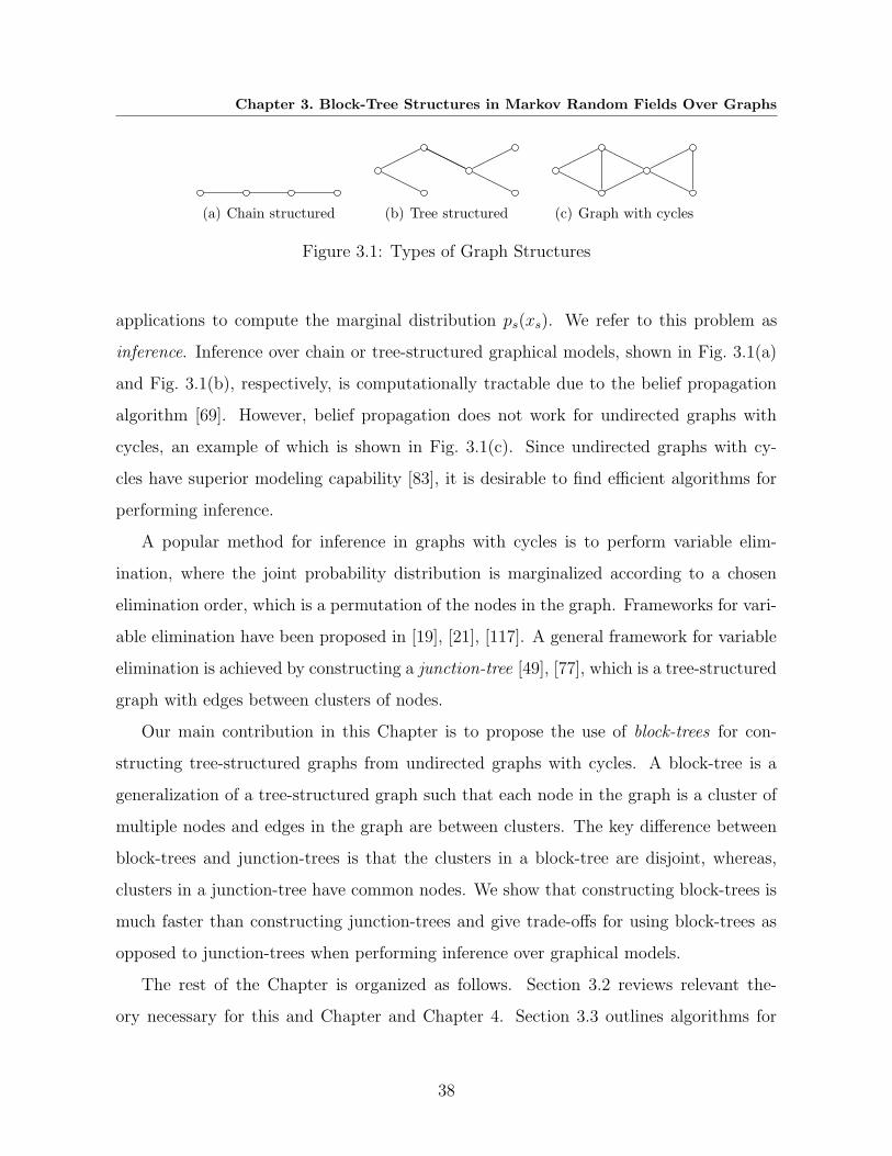
Chapter 3. Block-Tree Structures in Markov Random Fields Over Graphs
(a) Chain structured (b) Tree structured (c) Graph with cycles
Figure 3.1: Types of Graph Structures
applications to compute the marginal distribution ps(xs). We refer to this problem as
inference. Inference over chain or tree-structured graphical models, shown in Fig. 3.1(a)
and Fig. 3.1(b), respectively, is computationally tractable due to the belief propagation
algorithm [69]. However, belief propagation does not work for undirected graphs with
cycles, an example of which is shown in Fig. 3.1(c). Since undirected graphs with cy-
cles have superior modeling capability [83], it is desirable to find efficient algorithms for
performing inference.
A popular method for inference in graphs with cycles is to perform variable elim-
ination, where the joint probability distribution is marginalized according to a chosen
elimination order, which is a permutation of the nodes in the graph. Frameworks for vari-
able elimination have been proposed in [19], [21], [117]. A general framework for variable
elimination is achieved by constructing a junction-tree [49], [77], which is a tree-structured
graph with edges between clusters of nodes.
Our main contribution in this Chapter is to propose the use of block-trees for con-
structing tree-structured graphs from undirected graphs with cycles. A block-tree is a
generalization of a tree-structured graph such that each node in the graph is a cluster of
multiple nodes and edges in the graph are between clusters. The key difference between
block-trees and junction-trees is that the clusters in a block-tree are disjoint, whereas,
clusters in a junction-tree have common nodes. We show that constructing block-trees is
much faster than constructing junction-trees and give trade-offs for using block-trees as
opposed to junction-trees when performing inference over graphical models.
The rest of the Chapter is organized as follows. Section 3.2 reviews relevant the-
ory necessary for this and Chapter and Chapter 4. Section 3.3 outlines algorithms for
38

3.2. Background and Problem Statement
constructing block-trees given a graph. Section 3.4 shows how the belief propagation algo-
rithm can be extended for inference over block-trees. Section 3.5 discusses the advantages
of using block-trees vs. junction-trees for inference over graphical models. Section 3.6
summarizes the Chapter.
3.2 Background and Problem Statement
Section 3.2.1 reviews properties and definitions related to graphs and graphical models
necessary for this Chapter. For a more complete study, we refer to [48]. Section 3.2.2
defines the problem of inference over graphical models. Section 3.2.3 outlines the belief
propagation algorithm for inference over tree-structured graphical models. Section 3.2.4
outlines the junction-tree algorithm for inference over undirected graphs with cycles. Sec-
tion 3.2.5 outlines our problem statement for constructing block-trees.
3.2.1 Graphs and Graphical Models
Let x = xs ∈ Rd : s ∈ V be a random vector defined on a graph G = (V,E), where
V = 1, 2, . . . , n is the set of nodes and E ⊂ V × V is the set of edges. For notational
simplicity we assume that d = 1, so that each node in the graph is a random variable.
Our results easily generalize to the case when d > 1. Given any subset W ⊂ V , let
xW = xs : s ∈W
denote the set of random variables in W . An edge between two nodes can either be
directed, denoted by s→ t, or undirected, denoted by s− t. One way of representing the
edge set is via an n× n adjacency matrix A such that
A(i, j) = 1 if (i, j) ∈ E , (3.1)
where we assume A(i, i) = 1 for all i = 1, . . . , n. If (s, t) is a directed edge, xs is called
a parent of xt and xt is called a child of xs. Denote the set of all parents of a node xs
39
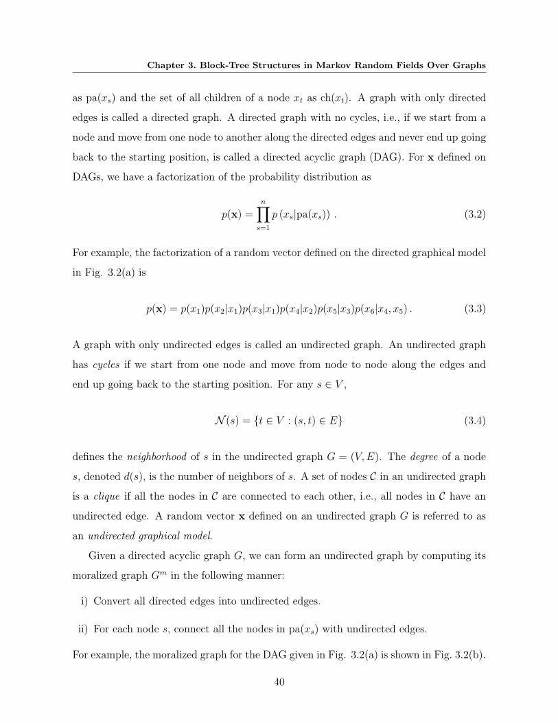
Chapter 3. Block-Tree Structures in Markov Random Fields Over Graphs
as pa(xs) and the set of all children of a node xt as ch(xt). A graph with only directed
edges is called a directed graph. A directed graph with no cycles, i.e., if we start from a
node and move from one node to another along the directed edges and never end up going
back to the starting position, is called a directed acyclic graph (DAG). For x defined on
DAGs, we have a factorization of the probability distribution as
p(x) =n∏
s=1
p (xs|pa(xs)) . (3.2)
For example, the factorization of a random vector defined on the directed graphical model
in Fig. 3.2(a) is
p(x) = p(x1)p(x2|x1)p(x3|x1)p(x4|x2)p(x5|x3)p(x6|x4, x5) . (3.3)
A graph with only undirected edges is called an undirected graph. An undirected graph
has cycles if we start from one node and move from node to node along the edges and
end up going back to the starting position. For any s ∈ V ,
N (s) = t ∈ V : (s, t) ∈ E (3.4)
defines the neighborhood of s in the undirected graph G = (V,E). The degree of a node
s, denoted d(s), is the number of neighbors of s. A set of nodes C in an undirected graph
is a clique if all the nodes in C are connected to each other, i.e., all nodes in C have an
undirected edge. A random vector x defined on an undirected graph G is referred to as
an undirected graphical model.
Given a directed acyclic graph G, we can form an undirected graph by computing its
moralized graph Gm in the following manner:
i) Convert all directed edges into undirected edges.
ii) For each node s, connect all the nodes in pa(xs) with undirected edges.
For example, the moralized graph for the DAG given in Fig. 3.2(a) is shown in Fig. 3.2(b).
40
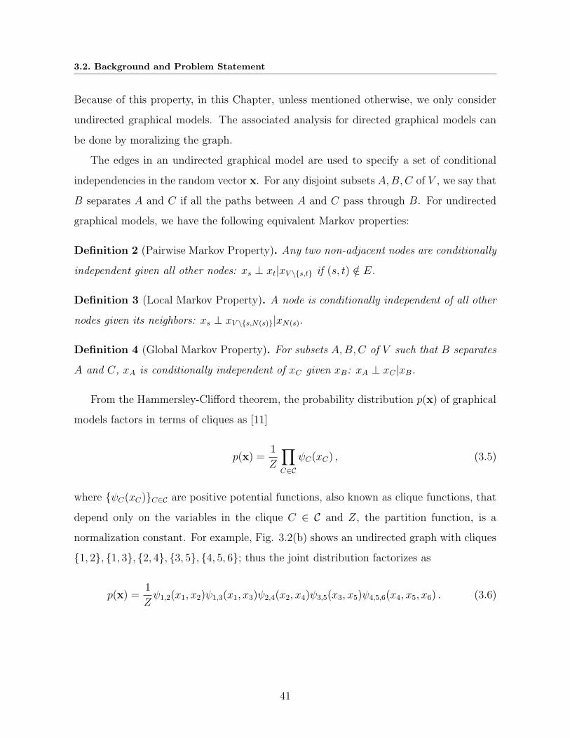
3.2. Background and Problem Statement
Because of this property, in this Chapter, unless mentioned otherwise, we only consider
undirected graphical models. The associated analysis for directed graphical models can
be done by moralizing the graph.
The edges in an undirected graphical model are used to specify a set of conditional
independencies in the random vector x. For any disjoint subsets A,B,C of V , we say that
B separates A and C if all the paths between A and C pass through B. For undirected
graphical models, we have the following equivalent Markov properties:
Definition 2 (Pairwise Markov Property). Any two non-adjacent nodes are conditionally
independent given all other nodes: xs ⊥ xt|xV \s,t if (s, t) /∈ E.
Definition 3 (Local Markov Property). A node is conditionally independent of all other
nodes given its neighbors: xs ⊥ xV \s,N(s)|xN(s).
Definition 4 (Global Markov Property). For subsets A,B,C of V such that B separates
A and C, xA is conditionally independent of xC given xB: xA ⊥ xC |xB.
From the Hammersley-Clifford theorem, the probability distribution p(x) of graphical
models factors in terms of cliques as [11]
p(x) =1
Z
∏
C∈C
ψC(xC) , (3.5)
where ψC(xC)C∈C are positive potential functions, also known as clique functions, that
depend only on the variables in the clique C ∈ C and Z, the partition function, is a
normalization constant. For example, Fig. 3.2(b) shows an undirected graph with cliques
1, 2, 1, 3, 2, 4, 3, 5, 4, 5, 6; thus the joint distribution factorizes as
p(x) =1
Zψ1,2(x1, x2)ψ1,3(x1, x3)ψ2,4(x2, x4)ψ3,5(x3, x5)ψ4,5,6(x4, x5, x6) . (3.6)
41

Chapter 3. Block-Tree Structures in Markov Random Fields Over Graphs
1
2
3
4
5
6
(a) Directed graph
1
2
3
4
5
6
(b) Undirected graph
Figure 3.2: Different examples of graphical models
3.2.2 Inference Algorithms
Inference in graphical models corresponds to finding marginal distributions, say ps(xs),
given the probability distribution p(x) for x = x1, . . . , xn. Assuming xs is a discrete
random variable taking values in Ω such that |Ω| = K, we have
ps(xs) =∑
xk∈Ω,k=1,...,n,k 6=s
p(x) . (3.7)
Computing ps(xs) using (3.7) requires Kn−1 additions since there are n− 1 joint summa-
tions over K possible states of xs. Further, these additions must be done for each state of
xs, thus the total complexity is O(Kn). Even for small K, for example if Ω is binary, i.e.,
Ω = 0, 1, computing marginals becomes computationally challenging. For graphical
models, this problem is simplified since p(x) admits a factorization, such as in (3.2) or
(3.5). As an example, consider the undirected graph in Fig. 3.2(b), and suppose we want
to compute p6(x6). Given p(x) as in (3.6), we have
p6(x6) =1
Z
∑
x1,x2,x3,x4,x5
ψ1,2ψ1,3ψ2,4ψ3,5ψ4,5,6 , (3.8)
where ψA(xA) is shortened as ψA. We can distribute the computations in (3.8) as follows:
p6(x6) =∑
x4,x5
[ψ4,5,6
(∑
x3
ψ3,5
)(∑
x2
ψ2,4
(∑
x1
ψ1,2ψ1,3
))]. (3.9)
Using (3.8) for computing p6(x6) requires K6 additions, whereas, using (3.9) requires
4K3 additions. Using (3.9) to compute marginals is known as variable elimination and
42

3.2. Background and Problem Statement
general frameworks for doing this have been proposed in [21], [117]. The key step in
variable elimination over graphs is to choose an elimination order, which is a permutation
of nodes. For example, in (3.9), the elimination order is 1, 2, 3, 4, 5, 6. The marginal
computed is always at the end of the order. The complexity of the variable elimination
algorithm depends on the elimination order. An optimal elimination order is the one that
results in the least number of summations. The problem of finding an optimal elimination
order can be mapped to finding the treewidth (see Definition 6) of a graph, which is an
NP-hard problem [5]. The variable elimination algorithm has a hidden step where we
triangulate a graph. A triangulated graph, also known as a chordal graph, is defined as
follows [101]:
Definition 5 (Triangulated graph). A graph is triangulated if all cycles of length four or
more have an edge connecting non-adjacent nodes in the cycle.
For example, in (3.9), when summing over x1, the resulting term∑
x1ψ1,2 ψ1,3 is a
function of the nodes x2 and x3 and thus creating an edge between these two nodes.
Each summation in the variable elimination algorithm creates intermediate factors. We
can capture these factors graphically using the triangulation algorithm, which has the
following steps [8]:
1. Choose an elimination order, which is a permutation of nodes in the graph.
2. For each node in the elimination order, form an edge between all the nodes in its
neighbors and update the edge set.
3. Remove the node and all its edges to other nodes and repeat step 2 until we exhaust
all the nodes in the elimination order.
The resulting graph after steps 1-3 will be triangulated. Using the triangulated graph,
we define the width and treewidth as follows [77].
Definition 6 (Width and Treewidth). Width of a triangulated graph is the size of the
largest clique minus 1. Treewidth, tw(G), of a graph G is the minimum width among all
possible triangulations of the graph G.
43

Chapter 3. Block-Tree Structures in Markov Random Fields Over Graphs
The complexity of variable elimination, given an elimination order, is exponential in
the width. So, finding an optimal elimination order corresponds to finding the treewidth of
a given graph, which is an NP-hard problem. Thus, it is desirable to have a low treewidth
graph to recover computationally tractable algorithms on graphical models. An example
of a low treewidth graph are trees, that have treewidth of one.
A limitation of the variable elimination algorithm is that it does not scale well when
more than one marginal density needs to be computed. For this purpose, message passing
algorithms have been proposed in the literature. For tree-structured graphs, we review
the belief propagation algorithm next in Section 3.2.3.
3.2.3 Belief Propagation
The belief propagation algorithm consists of the following steps [69]:
1. Identify a root node, say xr, and find all the nodes other than xr which have degree
one. These are called the leaves of the tree.
2. Starting from the leaves, pass messages along edges in the graph until we reach the
root node xr:
mi→j =∑
xi
ψi,j(xi, xj)∏
e∈N (i)\j
me→j , (3.10)
where mi→j indicates the message passed from node xi to xj.
3. Once all the messages reach the root node xr, pass messages starting from xr to all
the leaves in the same way as done in step 2 using (3.10).
Fig. 3.3 shows an example of how the belief propagation algorithm works. The
marginal probability distribution of each node is the product of all messages received
from its neighbors, i.e.,
p(xs) =1
Z
∏
t∈N (s)
mt→s . (3.11)
In this way, we avoid the need to do variable elimination repeatedly for computing the
marginal distribution of each node in the graph. The above algorithm only works for
44

3.2. Background and Problem Statement
1
2 3
4 5 6 7
(a)
1
2 3
4 5 6 7
(b)
Figure 3.3: Belief propagation on trees: (a) messages, shown via dashed lines, are firstpassed from the leaves to the root, (b) and then passed from the root to the leaves.
tree and chain structured distributions. For graphs with cycles, a popular method is to
construct a junction-tree and then apply belief propagation, which we discuss in the next
Section.
3.2.4 Junction-Tree
Junction-trees were introduced in [77] for representing graphs with cycles as tree-structured
graphs. In [49], the authors showed that inference in graphical models with cycles can be
achieved efficiently using junction-trees. Formally, a junction-tree is defined as follows.
Definition 7 (Junction-Tree). For a graph G = (V,E), a junction-tree J = (C, E) is a
graph over clusters of nodes in V so that
1. Each node in V is associated with at least one cluster in C.
2. For every edge (v1, v2) ∈ E, there exists a cluster Ck ∈ C such that v1, v2 ∈ Ck.
3. J satisfies the running intersection property: For all clusters Ci, Ck, and Cj such
that Ck separates Ci and Cj, Ci ∩ Cj ⊂ Ck.
The idea behind using junction-trees for inference in graphical models is to cluster
nodes in the graph and then form a tree-structured graph over the clusters. Given a
tree-structured graph, we can now apply variants of the belief propagation algorithm so
that the message passing is between clusters of nodes (instead of individual nodes) [34],
[82]. The running intersection property ensures that inference over the junction-tree is
45

Chapter 3. Block-Tree Structures in Markov Random Fields Over Graphs
Algorithm 1: Constructing a Junction-Tree: JunctionTree(G,W )
Data: A graph G = (V,E) and an elimination order W .Result: A junction-tree J = (C, E)
1 Triangulate the graph G using the elimination order W .2 Identify the set of cliques C in the triangulated graph.3 For all tuples Ci, Cj ∈ C, construct a weighted graph with weightsw(i, j) = |Ci ∩ Cj|.
4 E ← arg maxE
∑
(i,j)∈E
w(i, j).
1
2 3
4
(a)
1 31 2
2 4 3 4
(b)
1 2 3
2 3 4
(c)
Figure 3.4: (a) An undirected graph, (b) Not a valid junction-tree since 1, 2 separates 1, 3
and 3, 4,but 3 /∈ 1, 2. In other words, the running intersection property says that for two
clusters with a common node, all the clusters on the path between the two clusters must have
that common node. (c) A valid junction-tree for the graph in (a).
consistent so that if a node s is in two clusters, the marginal distribution of xs computed
from each cluster after running message passing is the same. Fig. 3.4 illustrates an example
of the running intersection property.
The next natural question to ask is how do we construct junction-trees and whether
there exists a junction-tree given an undirected graph. Note that if we simply assume
that the cluster in the junction-tree is all the nodes V of the original graph, we get a valid
junction-tree. This shows that a junction-tree always exists. An algorithm to construct a
junction-tree is outlined in Algorithm 1. In summary, we first triangulate a graph using
an elimination order, then find the cliques in the triangulated graph, and then use a
maximum weight spanning tree (MWST) algorithm to find an appropriate tree over the
cliques.
Theorem 3.2.1. Given a graph G = (V,E), the complexity of constructing a junction-
46

3.2. Background and Problem Statement
tree (Algorithm 1) given an elimination order W is O(|E|+ |C|2), where C are the cliques
in the triangulated graph computed using the elimination order W .
Proof. Triangulation has complexity O(|E|) [78]. Given a triangulated graph with |C|
number of clusters, we need to find the weighted graph, which has complexity O(|C|2)
and the MWST algorithm has a worst case complexity of O(|C|2) [33].
To do inference using the junction tree, we first associate potential functions with each
clique. This is done by grouping potentials from the original joint distribution and map-
ping them to their respective cliques. Having defined potential functions for each clique,
a message passing scheme, similar in spirit to the belief propagation algorithm outlined
in Section 3.2.3, can be formulated to compute marginal distributions for each clique [34],
[49], [82]. The marginal distribution of each node can be subsequently computed by
marginalizing the distribution of the cliques. The following theorem summarizes the
complexity of performing belief propagation over graphical models using junction-trees.
Theorem 3.2.2 (Complexity of inference using junction tree). For a random vector
x ∈ Ωn, where |Ω| = K, defined on an undirected graph G = (V,E), the complexity of
message passing using a junction-tree J = (C, E) is
O
∑
(i,j)∈E
K |Ci| +K |Cj |
. (3.12)
In Theorem 3.2.2, when K is large compared to |C|, the complexity of inference will
be dominated by the clique with maximum size. Thus, an optimal junction-tree can be
defined as the junction-tree with minimal maximal clique size. In Definition 6, we saw
that this is equivalent to defining the treewidth of a graph, which in turn corresponds to
finding an optimal elimination order. Further, since finding the optimal elimination order
is an NP-hard problem, finding an optimal junction tree is also NP-hard.
We now consider some examples of how junction-trees are constructed. The examples
presented here will be used later to show how our proposed framework for using block-trees
compares to that of using junction-trees.
47
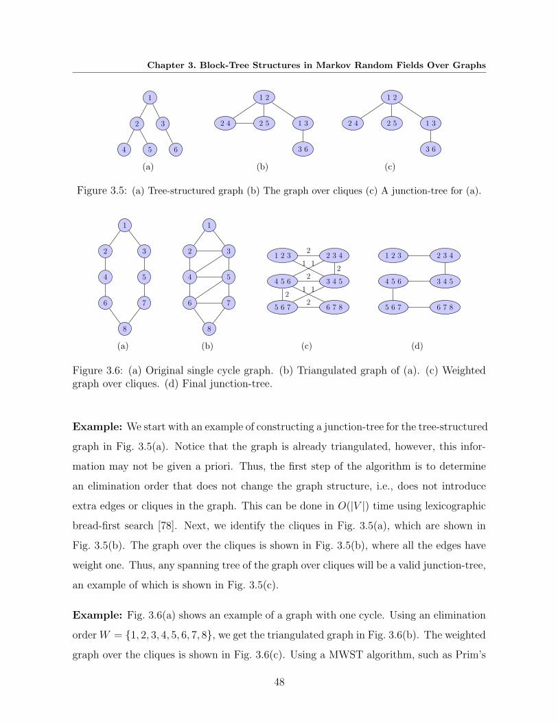
Chapter 3. Block-Tree Structures in Markov Random Fields Over Graphs
1
2 3
4 5 6
(a)
1 2
2 4 2 5 1 3
3 6
(b)
1 2
2 4 2 5 1 3
3 6
(c)
Figure 3.5: (a) Tree-structured graph (b) The graph over cliques (c) A junction-tree for (a).
1
2 3
4 5
6 7
8
(a)
1
2 3
4 5
6 7
8
(b)
1 2 3 2 3 4
3 4 54 5 6
5 6 7 6 7 8
2
12
1
2
211
2
(c)
1 2 3 2 3 4
3 4 54 5 6
5 6 7 6 7 8
(d)
Figure 3.6: (a) Original single cycle graph. (b) Triangulated graph of (a). (c) Weightedgraph over cliques. (d) Final junction-tree.
Example: We start with an example of constructing a junction-tree for the tree-structured
graph in Fig. 3.5(a). Notice that the graph is already triangulated, however, this infor-
mation may not be given a priori. Thus, the first step of the algorithm is to determine
an elimination order that does not change the graph structure, i.e., does not introduce
extra edges or cliques in the graph. This can be done in O(|V |) time using lexicographic
bread-first search [78]. Next, we identify the cliques in Fig. 3.5(a), which are shown in
Fig. 3.5(b). The graph over the cliques is shown in Fig. 3.5(b), where all the edges have
weight one. Thus, any spanning tree of the graph over cliques will be a valid junction-tree,
an example of which is shown in Fig. 3.5(c).
Example: Fig. 3.6(a) shows an example of a graph with one cycle. Using an elimination
order W = 1, 2, 3, 4, 5, 6, 7, 8, we get the triangulated graph in Fig. 3.6(b). The weighted
graph over the cliques is shown in Fig. 3.6(c). Using a MWST algorithm, such as Prim’s
48

3.2. Background and Problem Statement
1 2 3
4 5 6
7 8 9
(a)
1 2 3
4 5 6
7 8 9
(b)
1 2 4
2 4 5 8
4 7 8
2 5 6 8
2 3 6
6 8 9
1 1
2
1
1
3
2
1
1
1
1
2
2
(c)
1 2 4
2 4 5 8
4 7 8
2 5 6 8
2 3 6
6 8 9
(d)
Figure 3.7: (a) A grid graph (b) Triangulated graph of (a). (c) Weighted graph over cliques.
(d) Junction-tree
[74] or Kruskal’s [47], we get the junction-tree in Fig. 3.6(d). It can easily be shown that
this junction-tree is optimal, i.e., there exists no other junction-tree with smaller maximal
clique size.
Example: Consider the 3×3 grid graph in Fig. 3.7(a). A triangulated graph, constructed
using the elimination order 1, 3, 7, 9, 4, 5, 2, 6, 8, is shown in Fig. 3.7(b). It can be
shown that the elimination order chosen is optimal. The weighted graph over cliques is
shown in Fig. 3.7(c). The junction tree constructed using the triangulated graph is shown
in Fig. 3.7(d). The width of the triangulated graph in Fig. 3.7(c) is three. Since the
elimination order is optimal, the treewidth of the graph in Fig. 3.7(a) is also three.
Example: By deleting the edge between node 1 and 2 in Fig. 3.7(a), we consider
the partial grid graph in Fig. 3.8(a). Fig. 3.8(b) shows the triangulated graph using an
optimal elimination order 1, 3, 7, 9, 4, 5, 2, 6, 8. The weighted graph over cliques is shown
in Fig. 3.8(c). Using this weighted graph, two possible junction-trees can be constructed,
which are shown in Fig. 3.8(d) and Fig. 3.8(e), respectively. This example shows that
given an elimination order, the corresponding junction-tree may not be unique.
49
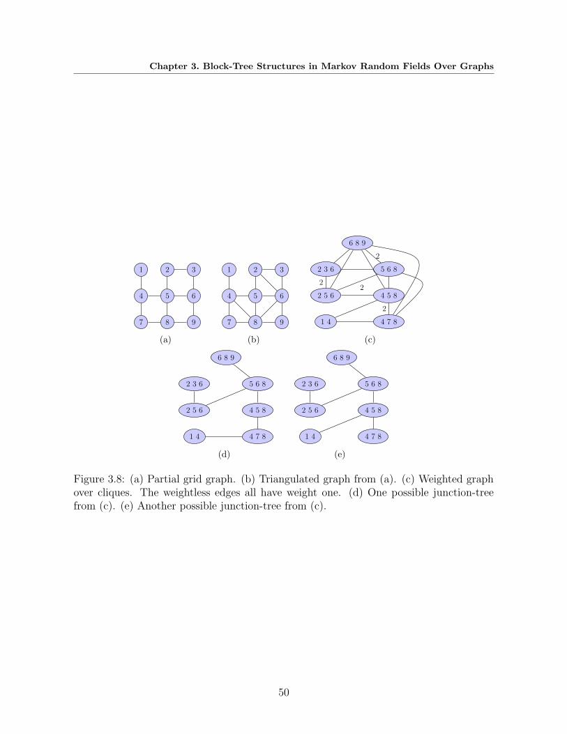
Chapter 3. Block-Tree Structures in Markov Random Fields Over Graphs
1 2 3
4 5 6
7 8 9
(a)
1 2 3
4 5 6
7 8 9
(b)
6 8 9
2 3 6 5 6 8
2 5 6 4 5 8
1 4 4 7 8
2
22
2
(c)
6 8 9
2 3 6 5 6 8
2 5 6 4 5 8
1 4 4 7 8
(d)
6 8 9
2 3 6 5 6 8
2 5 6 4 5 8
1 4 4 7 8
(e)
Figure 3.8: (a) Partial grid graph. (b) Triangulated graph from (a). (c) Weighted graphover cliques. The weightless edges all have weight one. (d) One possible junction-treefrom (c). (e) Another possible junction-tree from (c).
50
3.2. Background and Problem Statement
3.2.5 Problem Statement
In this Chapter, we consider an alternative to junction-trees for deriving efficient inference
algorithms over graphical models. Instead of using junction-trees, we propose block-trees,
that are defined as follows.
Definition 8 (Block-Tree). For a graph G = (V,E), a block-tree G = (V , E) is a graph
over clusters of nodes in V such that
1. Each node in V is associated with only one cluster in V. In other words, the clusters
in V are disjoint.
2. The edges E ⊂ |V| × |V| form a tree-structured graph.
Note that the main difference between a block-tree and junction-tree is that a junction-
tree is a tree-structured graph on overlapping clusters, whereas the clusters in a block-tree
are disjoint. Further, in defining edges in a junction-tree, it is important to satisfy the
running intersection property, whereas, there is no such requirement for defining block-
trees.
We propose an O(|E|) algorithm for constructing block-trees. This makes construct-
ing block-trees faster than constructing junction-trees, thus making block-trees a practical
alternative to junction-trees when solving inference problems over graphical models. Nu-
merically, we show that for a certain class of graphs, using block-trees for inference is
computationally faster than using junction-trees. This is mainly true for graphical mod-
els in which exact inference is computationally tractable. In Chapter 4, we will show how
block-trees can be used to derive efficient approximate inference algorithms over arbitrary
graphical models.
There has been work in deriving efficient algorithms on graphical models using disjoint
clusters. In fact, it is well known that inference over graphical models can be performed
using disjoint clustering, and researchers often refer to this as the clustering algorithm
and credit the book by J.D. Pearl [69]. Specific applications of using disjoint clustering
in medical diagnostics can be found in [17] and [71]. In the engineering literature, [110]
51
Chapter 3. Block-Tree Structures in Markov Random Fields Over Graphs
and [62] derive recursive representations by scanning the lattice horizontally (or vertically)
and thereby forming disjoint clusters of nodes. To our knowledge, previous work has not
addressed the question of constructing a block-tree given an arbitrary graph. Further, our
analysis shows how block-trees compare to junction-trees and how block-trees can lead to
computationally faster algorithms for inference over a certain class of graphical models.
3.3 Tree Structures in Graphs Using Block-Trees
In this Section, we show how block-trees can be used to find tree structures in arbitrary
graphs and present various examples of this construction. Section 3.3.1 outlines an algo-
rithm for constructing block-trees given an arbitrary graphs. Section 3.3.2 shows how to
construct block-trees in linear time. Section 3.3.3 compares block-trees to junction-trees.
3.3.1 Constructing Block-Trees
Suppose we are given an undirected graph G = (V,E), where |V | = n. Given G, we want
to find a block-tree G = (V , E) such that V = V1,V2, . . . ,Vl is a set of disjoint clusters
and E is a set of edges such that (i, j) ∈ E if there exists an edge e ∈ E between any node
in Vi and any node in Vj.
Our proposed algorithm for constructing G is shown in Algorithm 2. The input to the
algorithm is the original graph G and a set of nodes V1 ⊂ V . The output of the algorithm
is the block-tree G. We refer to V1 as the root cluster. The various steps in the algorithm
are explained as follows:
• Forward step (Line 1): We find clusters V1, V2, . . . , Vr using breadth-first search
(BFS). These clusters serve as initial clusters for the block-tree.
• Let E ′ be a copy of the edges E (Line 2) and let denote G′ = (V,E ′).
• Split Vr into its connected components V 1r , . . . , V
mrr using the subgraph G(Vr),
which denotes the graph only over the nodes in Vr (Line 3).
52

3.3. Tree Structures in Graphs Using Block-Trees
Algorithm 2: Constructing Block-Trees: BlockTree(G,V1)
Data: A graph G = (V,E) and a set of nodes V1.Result: A block-tree G = (C, E)
1 Find successive neighbors of V1 to construct a sequence of r clusters V1, V2, . . . , Vr
such that V2 = N (V1), V3 = N (V2)\V1 ∪ V2, . . . , Vr = N (Vr)\Vr−2 ∪ Vr−1.2 E ′ ← E3 V 1
r , . . . , Vmrr ← Find mr connected components of Vr using subgraph G(Vr).
4 for i = r, r − 1, . . . 2 do5 for j = 1, 2, . . . mi do
6 C(V ji )← N (V j
i ) ∩ Vi−1 ; All nodes in Vi connected to V ji .
7 Update E ′ with all the edges between nodes in C(V ji ).
8 V 1i−1, . . . , V
mi−1
i−1 ← Find mi−1 connected components of Vi−1 using subgraphG′(Vi−1).
9 V 11 , . . . , V
m1
1 ← Find m1 connected components of V1 using subgraph G(V1).10 V ←
⋃rk=1V
1k , V
2k , . . . , V
mk
k 11 E ← edges between all the clusters in C
• Backwards step (Lines 3-7): We now recursively split other clusters. Starting at
k = r, for each connected component V jr of Vr, find the set of nodes C(V j
r ) that are
connected to Vr−1 (Line 6). Next, we find all possible edges over the nodes C(V jr )
and add these edges to E ′ (Line 7). These edges indicate the nodes in Vr−1 that
should belong to the same cluster, i.e., if there exists an edge between v, v ′ ∈ Vr−1,
v and v′ would belong to the same cluster in the final block-tree. Find all connected
components of Vr−1 (Line 8). Repeat the above steps for k = r − 1 till k = 2.
• Split V1 into connected components using the graph G(V1) (Line 9).
• After splitting the clusters Vk for k = 1, 2, . . . , r, we find the associated block-tree
(Lines 10 and 11).
We illustrate Algorithm 2 using some examples.
Example: Consider the tree-structured graph in Fig. 3.5(a). Suppose we choose V1 =
1. Using the structure of the graph, we have that V2 = 2, 3, V3 = 4, 5, 6. We
now find the components of V3 in G(V3). It is clear that G(V3) is edgeless, so that
53
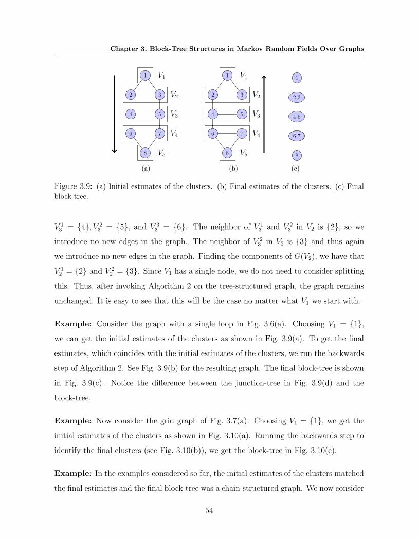
Chapter 3. Block-Tree Structures in Markov Random Fields Over Graphs
1
2 3
4 5
6 7
8
V1
V2
V3
V4
V5
(a)
1
2 3
4 5
6 7
8
V1
V2
V3
V4
V5
(b)
1
2 3
4 5
6 7
8
(c)
Figure 3.9: (a) Initial estimates of the clusters. (b) Final estimates of the clusters. (c) Final
block-tree.
V 13 = 4, V 2
3 = 5, and V 33 = 6. The neighbor of V 1
3 and V 23 in V2 is 2, so we
introduce no new edges in the graph. The neighbor of V 23 in V2 is 3 and thus again
we introduce no new edges in the graph. Finding the components of G(V2), we have that
V 12 = 2 and V 2
2 = 3. Since V1 has a single node, we do not need to consider splitting
this. Thus, after invoking Algorithm 2 on the tree-structured graph, the graph remains
unchanged. It is easy to see that this will be the case no matter what V1 we start with.
Example: Consider the graph with a single loop in Fig. 3.6(a). Choosing V1 = 1,
we can get the initial estimates of the clusters as shown in Fig. 3.9(a). To get the final
estimates, which coincides with the initial estimates of the clusters, we run the backwards
step of Algorithm 2. See Fig. 3.9(b) for the resulting graph. The final block-tree is shown
in Fig. 3.9(c). Notice the difference between the junction-tree in Fig. 3.9(d) and the
block-tree.
Example: Now consider the grid graph of Fig. 3.7(a). Choosing V1 = 1, we get the
initial estimates of the clusters as shown in Fig. 3.10(a). Running the backwards step to
identify the final clusters (see Fig. 3.10(b)), we get the block-tree in Fig. 3.10(c).
Example: In the examples considered so far, the initial estimates of the clusters matched
the final estimates and the final block-tree was a chain-structured graph. We now consider
54
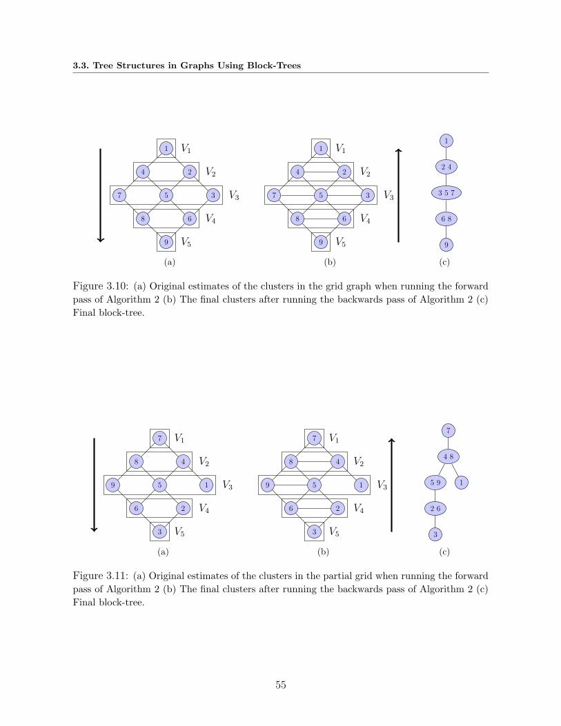
3.3. Tree Structures in Graphs Using Block-Trees
1
4 2
7 5 3
8 6
9
V1
V2
V3
V4
V5
(a)
1
4 2
7 5 3
8 6
9
V1
V2
V3
V4
V5
(b)
1
2 4
3 5 7
6 8
9
(c)
Figure 3.10: (a) Original estimates of the clusters in the grid graph when running the forward
pass of Algorithm 2 (b) The final clusters after running the backwards pass of Algorithm 2 (c)
Final block-tree.
7
8 4
9 5 1
6 2
3
V1
V2
V3
V4
V5
(a)
7
8 4
9 5 1
6 2
3
V1
V2
V3
V4
V5
(b)
7
4 8
5 9 1
2 6
3
(c)
Figure 3.11: (a) Original estimates of the clusters in the partial grid when running the forward
pass of Algorithm 2 (b) The final clusters after running the backwards pass of Algorithm 2 (c)
Final block-tree.
55
Chapter 3. Block-Tree Structures in Markov Random Fields Over Graphs
an example where the final block-tree will in fact be tree-structured. Consider the partial
grid graph of Fig. 3.8(a). Choosing V1 = 7, we get the initial estimates of the clusters
in Fig. 3.11(a). We now run the backwards step of the algorithm. Since V5 has only
one node, we do not need to find its components. Now, V5 is connected to 2 and 6, so
C(V5) = 2, 6. We introduce an edge between 2 and 6 to show that both 2 and 6 should
be in the same cluster in the final block-tree. Next, we find the components of V4 using
the additional edges and the component is V4 itself. Now, V4 is connected to both 5 and
9 in V3, so C(V4) = 5, 9. We introduce an edge between 5 and 9 and then find the
connected components of V3. Notice that 1 is not connected to 5 and 9, so we can split V3
as V 13 = 5, 9 and V 2
3 = 1. Continuing the algorithm we find the rest of the clusters
as shown in Fig. 3.11(c). The final block-tree is shown in Fig.3.11(d).
The examples above illustrate how to construct block-trees given an undirected graph.
As mentioned in Section 3.2.1, directed graphs can be converted to undirected graphs, so
the algorithm for constructing block-trees also extends to directed graphs.
3.3.2 A Linear Time Block-Tree Construction Algorithm
Algorithm 2 for constructing block-trees served as a way to explain the block-tree con-
struction algorithm. In this Section, we present an O(|E|) algorithm for constructing a
block-tree given an undirected graph G = (V,E) and an initial root cluster V1.
Step 1. Use a breadth-first-search (BFS) algorithm to construct clusters V1, V2, . . . , Vr as
in Line 1 of Algorithm 2. For each cluster Vk, split Vk into mk disjoint clusters
V 1k , . . . , V
mk
k such that⋃V k
k = Vk and there are no edges between V ik and V j
k for
i 6= j. This partitioning of the nodes can be done in O(|E|) time using standard
BFS algorithms.
Step 2. We now merge clusters to find the final block-tree. The key intuition in this
step is that each cluster in Vk should be connected to a single cluster in Vk−1.
If this is not the case, we merge clusters in Vk−1 accordingly. Starting at Vr =
V 1r , V
2r , . . . , V
mrr , for each V j
r , j = 1, . . . ,mr, find all clusters C(V jr ) in Vr−1
56
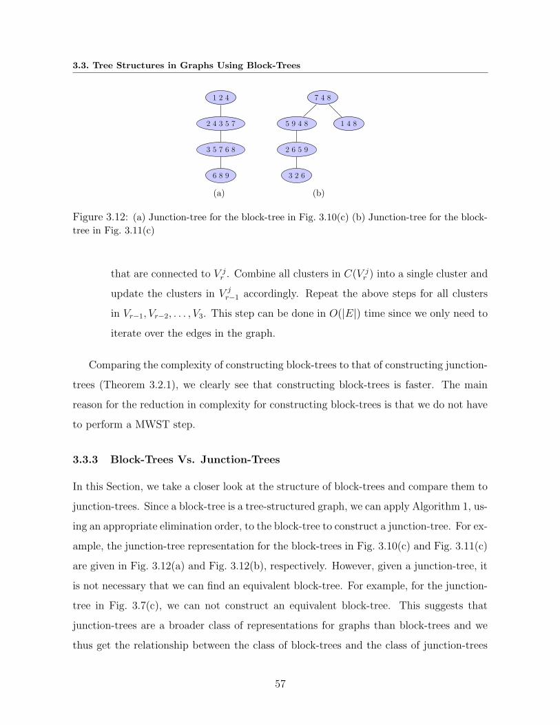
3.3. Tree Structures in Graphs Using Block-Trees
1 2 4
2 4 3 5 7
3 5 7 6 8
6 8 9
(a)
7 4 8
1 4 85 9 4 8
2 6 5 9
3 2 6
(b)
Figure 3.12: (a) Junction-tree for the block-tree in Fig. 3.10(c) (b) Junction-tree for the block-
tree in Fig. 3.11(c)
that are connected to V jr . Combine all clusters in C(V j
r ) into a single cluster and
update the clusters in V jr−1 accordingly. Repeat the above steps for all clusters
in Vr−1, Vr−2, . . . , V3. This step can be done in O(|E|) time since we only need to
iterate over the edges in the graph.
Comparing the complexity of constructing block-trees to that of constructing junction-
trees (Theorem 3.2.1), we clearly see that constructing block-trees is faster. The main
reason for the reduction in complexity for constructing block-trees is that we do not have
to perform a MWST step.
3.3.3 Block-Trees Vs. Junction-Trees
In this Section, we take a closer look at the structure of block-trees and compare them to
junction-trees. Since a block-tree is a tree-structured graph, we can apply Algorithm 1, us-
ing an appropriate elimination order, to the block-tree to construct a junction-tree. For ex-
ample, the junction-tree representation for the block-trees in Fig. 3.10(c) and Fig. 3.11(c)
are given in Fig. 3.12(a) and Fig. 3.12(b), respectively. However, given a junction-tree, it
is not necessary that we can find an equivalent block-tree. For example, for the junction-
tree in Fig. 3.7(c), we can not construct an equivalent block-tree. This suggests that
junction-trees are a broader class of representations for graphs than block-trees and we
thus get the relationship between the class of block-trees and the class of junction-trees
57
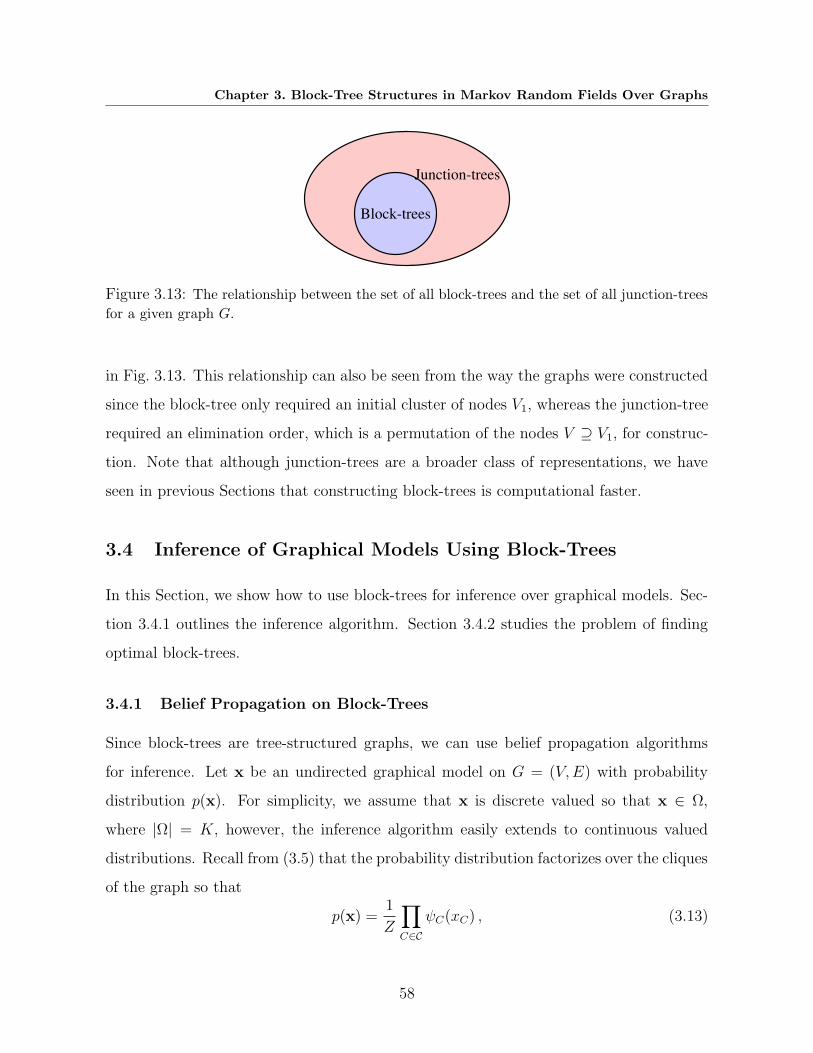
Chapter 3. Block-Tree Structures in Markov Random Fields Over Graphs
Junction-trees
Block-trees
Figure 3.13: The relationship between the set of all block-trees and the set of all junction-trees
for a given graph G.
in Fig. 3.13. This relationship can also be seen from the way the graphs were constructed
since the block-tree only required an initial cluster of nodes V1, whereas the junction-tree
required an elimination order, which is a permutation of the nodes V ⊇ V1, for construc-
tion. Note that although junction-trees are a broader class of representations, we have
seen in previous Sections that constructing block-trees is computational faster.
3.4 Inference of Graphical Models Using Block-Trees
In this Section, we show how to use block-trees for inference over graphical models. Sec-
tion 3.4.1 outlines the inference algorithm. Section 3.4.2 studies the problem of finding
optimal block-trees.
3.4.1 Belief Propagation on Block-Trees
Since block-trees are tree-structured graphs, we can use belief propagation algorithms
for inference. Let x be an undirected graphical model on G = (V,E) with probability
distribution p(x). For simplicity, we assume that x is discrete valued so that x ∈ Ω,
where |Ω| = K, however, the inference algorithm easily extends to continuous valued
distributions. Recall from (3.5) that the probability distribution factorizes over the cliques
of the graph so that
p(x) =1
Z
∏
C∈C
ψC(xC) , (3.13)
58

3.4. Inference of Graphical Models Using Block-Trees
where the functions ψC(xC) are known a priori. Suppose we construct a block-tree G =
(V , E) from G using a root cluster V1. To capture the structure of the original graph G
in the block-tree G, we introduce some notation. For every edge (i, j) ∈ E connecting two
clusters Vi and Vj, associate a label (V i,Vj) so that in the original graph G, the nodes in
V i are not connected to the nodes in V j. As an example, in Fig. 3.11(c), all the edge labels
will be empty, except the label between 1 and 4, 8, which will have a label (, 4).
The steps involved in inference over graphical models using block-trees are summarized
as follows.
Step 1. Construct a block-tree G from the undirected graph G using a root cluster V1.
Step 2. The cliques in the block-tree G are the edges, so we can write down an alternative
factorization for the probability distribution in p(x) as
p(x) =l∏
k=1
φk(xVk)∏
(i,j)∈E
Ψi,j(xVi\Vi, xVj\Vj
) , (3.14)
where we map each potential function in the original factorization in (3.13) to an
appropriate factor without repeating.
Step 3. Using an arbitrary root node in the block-tree, identify the leaves and pass mes-
sages starting at the leaves up to the root:
mi→j(xVj) =
∑
xVi\Vi
Ψi,j(xVi\Vi, xVj\Vj
)∑
xVi
∏
k∈N (xVi)\xVj
φi(xVi)mk→i(xVi
) (3.15)
Step 4. Once all messages have reached the root, pass messages from the root back to the
leaves using the same message passing equation in (3.15).
Step 5. The joint distribution for each cluster is given by
pVi(xVi
) =∏
j∈N (Vi)
mj→i(xVi)φi(xVi
) (3.16)
59
Chapter 3. Block-Tree Structures in Markov Random Fields Over Graphs
Step 6. Marginilize the distribution of each cluster to find the distribution of each node.
The complexity of the message passing algorithm is given as follows.
Theorem 3.4.1. For an undirected graphical model x defined on a graph G = (V,E),
let G = (V , E) be the block-tree constructed using a root cluster V1. The complexity of
message passing over the block-tree is
O
∑
(i,j)∈E
K |Vi| +K |Vj | + 2K |Vi\Vi|+|Vj\Vj |
. (3.17)
Proof. From (3.15), the complexity of passing messages from cluster Vi to cluster Vj is
O(K |Vi| +K |Vi\Vi|+|Vj\Vj |
). Summing over all edges and using the fact that we pass
messages twice on an edge (i, j), we get the desired result.
An alternative way to derive a message passing algorithm over block-trees is to trans-
form the block-tree into a junction-tree and then use popular junction-tree based inference
algorithms [34], [82]. The complexity of the inference algorithm will be the same, however,
by directly using the block-tree, we avoid the step of constructing a junction-tree. In the
next Section, we consider the problem of finding optimal block-trees.
3.4.2 Optimal Block-Trees
From Theorem 3.4.1, we see that the complexity of message passing over block-trees is
dominated by the term in (3.17) whose exponent is maximum. Thus, an optimal block-
tree can be defined such that the width
w(G, V1) = max(i,j)∈E
max
|V i|, |Vj|, |Vi\V i|+ |Vj\Vj|
(3.18)
is minimized. Notice that (3.18) depends on the choice of the root cluster V1 in con-
structing the block-tree. Thus, finding the optimal block-tree is equivalent to finding an
optimal root cluster. This problem is computationally intractable since we need to search
over all possible combinations of root clusters V1.
60

3.4. Inference of Graphical Models Using Block-Trees
7 4
8 5 1
9 6 2
3
V1
V2
V3
V4
(a)
7 4
8 5 1
9 6 2
3
(b)
7 4
8 5 1
9 6 2
3
(c)
Figure 3.14: (a) Original estimates of the clusters in the partial grid using V1 = 7, 4 as the
root cluster (b) Splitting of clusters (c) Final block-tree.
As an example illustrating how the choice of V1 alters the block-tree, consider finding
block-trees for the partial grid in Fig. 3.11. In Fig. 3.11(c), we construct a block-tree
using V1 = 7 as the root cluster. The complexity of inference in this graph is O(K4)
because of the message passing between the cluster 5, 9 and 4, 8 and between cluster
2, 6 and 5, 9. Instead of choosing V1 = 7, let V1 = 7, 4. The initial estimate of
the clusters are shown in Fig. 3.14(a). The final block-tree is shown in Fig. 3.14(c). It is
clear that message passing on the block-tree in Fig. 3.14(c) will have complexity O(K5)
because of the message passing between the cluster 9, 6, 2 and the cluster 8, 5.
3.4.3 Greedy Algorithms For Finding Optimal Block-Trees
In this Section, we discuss some greedy algorithms for finding optimal block-trees.
• Minimal degree node: In this approach, which we call MinDegree, we find the
node with minimal degree and use that node as the root cluster. The intuition
behind this is that the minimal degree node may lead to the smallest number of
nodes being added in the clusters. The complexity of this approach is O(n), where
n is the number of nodes in the graph.
• Using an elimination order: Recall from Section 3.3.3 that a block-tree can be
converted into a junction-tree by joining clusters connected via edges. This means
61
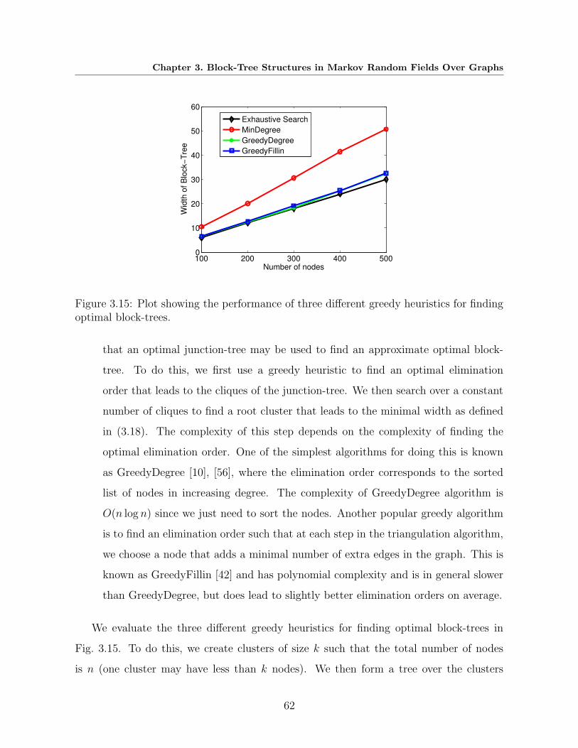
Chapter 3. Block-Tree Structures in Markov Random Fields Over Graphs
100 200 300 400 5000
10
20
30
40
50
60
Number of nodes
Wid
th o
f Blo
ck−T
ree
Exhaustive SearchMinDegreeGreedyDegreeGreedyFillin
Figure 3.15: Plot showing the performance of three different greedy heuristics for findingoptimal block-trees.
that an optimal junction-tree may be used to find an approximate optimal block-
tree. To do this, we first use a greedy heuristic to find an optimal elimination
order that leads to the cliques of the junction-tree. We then search over a constant
number of cliques to find a root cluster that leads to the minimal width as defined
in (3.18). The complexity of this step depends on the complexity of finding the
optimal elimination order. One of the simplest algorithms for doing this is known
as GreedyDegree [10], [56], where the elimination order corresponds to the sorted
list of nodes in increasing degree. The complexity of GreedyDegree algorithm is
O(n log n) since we just need to sort the nodes. Another popular greedy algorithm
is to find an elimination order such that at each step in the triangulation algorithm,
we choose a node that adds a minimal number of extra edges in the graph. This is
known as GreedyFillin [42] and has polynomial complexity and is in general slower
than GreedyDegree, but does lead to slightly better elimination orders on average.
We evaluate the three different greedy heuristics for finding optimal block-trees in
Fig. 3.15. To do this, we create clusters of size k such that the total number of nodes
is n (one cluster may have less than k nodes). We then form a tree over the clusters
62
3.5. Inference Over Graphical Models: Block-Tree Vs. Junction-Tree
and associate a clique between two clusters connected to each other. We then remove
a certain fraction of edges over the graph (not the block-tree), but make sure that the
graph is still connected. By construction, the width of the graph constructed will be at
most 2k. Fig. 3.15 shows the performance of MinDegee, GreedyDegree, and GreedyFillin
over graphs with different number of nodes and different values of k. We clearly see that
both GreedyDegree and GreedyFillin compute widths that are close to optimal. The main
point is that we can use various known algorithms for finding optimal junction-trees to
final optimal block-trees.
3.5 Inference Over Graphical Models: Block-Tree Vs. Junction-
Tree
In this Section, we show how block-trees can lead to computational savings when used
for inference over graphical models. The main idea is that for certain graphical models,
the complexity of constructing the junction-tree can dominate the complexity of the in-
ference algorithm, thus in these cases, we can use block-trees instead of junction-trees for
inference. Section 3.5.1 considers a simple example of a graphical model with a single
cycle and Section 3.5.2 considers more general graphical models.
3.5.1 Example: Single Cycle Graphical Models
Let G = (V,E) be a graphical model on a graph with a single cycle, as in Fig. 3.6(a).
The complexity of inference using a junction-tree is
O(n+ n2 + 2nK3
)≈ O
(n2 + 2nK3
), (3.19)
where O(n+ n2) is the complexity of constructing the junction-tree (see Theorem 3.2.1)
and O(nK3) is the complexity of belief propagation (see Theorem 3.2.2) since all the
cliques in the junction-tree will have size three (see Fig. 3.6(c) for an example). The
63
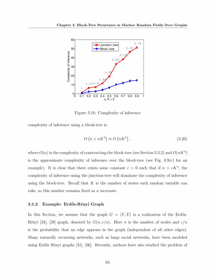
Chapter 3. Block-Tree Structures in Markov Random Fields Over Graphs
0 0.1 0.2 0.3 0.4 0.5 0.6 0.7 0.8 0.9 10
10
20
30
40
50
60
c, K = 2
Com
plex
ity o
f Inf
eren
ce
Junction−treeBlock−tree
1
1.19 1.61.86
1.99
2.03
2.15
2.33
2.79
Figure 3.16: Complexity of inference
complexity of inference using a block-tree is
O(n+ nK4
)≈ O
(nK4
), (3.20)
whereO(n) is the complexity of constructing the block-tree (see Section 3.3.2) andO(nK4)
is the approximate complexity of inference over the block-tree (see Fig. 3.9(c) for an
example). It is clear that there exists some constant c > 0 such that if n > cK4, the
complexity of inference using the junction-tree will dominate the complexity of inference
using the block-tree. Recall that K is the number of states each random variable can
take, so this number remains fixed as n increases.
3.5.2 Example: Erdos-Renyi Graph
In this Section, we assume that the graph G = (V,E) is a realization of the Erdos-
Renyi [24], [29] graph, denoted by G(n, c/n). Here n is the number of nodes and c/n
is the probability that an edge appears in the graph (independent of all other edges).
Many naturally occurring networks, such as large social networks, have been modeled
using Erdos Renyi graphs [31], [66]. Recently, authors have also studied the problem of
64
3.5. Inference Over Graphical Models: Block-Tree Vs. Junction-Tree
learning graphical models on sparse random graphs [3].
It is well known that for c < 1 and for large n, the treewidth of a graph realized using
an Erdos-Renyi model is at most two [23]. Thus, for graphical models defined on such
random graphs, inference is tractable. The comparison of the complexity of inference
using block-trees and junction-trees on a 1000 node graph is shown in Fig. 3.16. The
results shown are over 100 randomly generated graphs for c chosen between 0 and 1. The
average treewidth over the 100 graphs is also shown in the graph. We clearly see the
benefits of using block-trees over junction-trees. Note that, when reporting complexity
results, we factor in the complexity of constructing the junction-tree or the block-tree, in
addition to the complexity of performing message passing in the graph. For c > 1, the
graph realized using an Erdos-Renyi model no longer has low treewidth and the treewidth
is known to be of the order c′n, where c′ is some constant and n is the number of nodes in
the graph [50]. Thus, in this case, the complexity of inference will dominate the complexity
of constructing the junction-tree, so the block-tree framework will no longer be faster.
3.5.3 Discussion
From the examples presented in this Section, we see that, for a certain class of graphical
models, the complexity of using block-trees over junction-trees leads to complexity benefits
when performing inference over graphical models. The main computational gains are in
constructing the block-tree. We note that for some applications, the junction-tree or the
block-tree only needs to be computed once. In these cases, the complexity of inference
will be dominated by the message passing algorithm. Thus, the main advantage of the
block-tree framework is in studying inference problems where the graph structure varies
over time and the inference algorithm needs to compute a new tree-decomposition at each
time instant.
Fig. 3.17 outlines an algorithm for deciding between choosing the junction-tree or
block-tree for inference. In the first step of the algorithm, we compute an elimination
order from the graph. As outlined in Section 3.4.3, this can be done using standard
algorithms in the literature to compute optimal elimination orders, see [12] for a review
65

Chapter 3. Block-Tree Structures in Markov Random Fields Over Graphs
Elimination Order Triangulation
Block-Tree |C|2 > Kw(G)
Junction-TreeGW
C
C,GG
J
Yes
No
Figure 3.17: Algorithm to choose between a block-tree and a junction-tree for inference over
graphical models.
of such algorithms. Using the elimination order, we compute a triangulated graph and
find the set of cliques C. We use the set of cliques to find a block-tree as outlined in
Section 3.4.3. From the block-tree, we determine if the complexity of constructing the
junction-tree dominates the complexity of inference over the block-tree. If this is the case,
we use the block-tree for inference, otherwise we construct the junction-tree.
3.6 Summary
We introduced an alternative framework for performing inference over graphical models
using block-trees as opposed to using the popular approach of constructing junction-
trees. The key difference between a block-tree and junction-tree is that a block-tree
is a tree over disjoint clusters of nodes, whereas a junction-tree is a tree connecting
overlapping clusters of nodes. We showed that the complexity of constructing block-trees
is linear in the number of edges in the graph. This makes the construction of block-trees
faster than the construction of junction-trees. We derived message passing algorithms for
inference over block-trees that allowed us to define optimal block-trees. We proposed a
greedy heuristic for finding optimal block-trees that uses the cliques in the junction-tree.
Finally, we compared the complexity of using block-trees and junction-trees for inference.
We concluded that, when the complexity of constructing a junction-tree dominates the
complexity of performing inference using block-trees, the block-tree is a computationally
better framework for performing inference over graphical models. Further, this lead to an
algorithm for choosing between junction-trees and block-trees given the task of performing
66

3.6. Summary
inference over a graphical model on a graph G.
67

Chapter 3. Block-Tree Structures in Markov Random Fields Over Graphs
68
Chapter 4
Generalizing Algorithms on
Graphical Models Using
Block-Graphs
4.1 Introduction
In Chapter 3 we saw that exact inference over graphical models is computationally
tractable only for a particular class of graphical models with small treewidth. This severely
restricts the use of exact inference algorithms in real-world problems. For example, in
image processing, it is common to represent images as graphical models over lattices for
applications such as denoising and segmentation. However, the treewidth of an n × n
lattice is n and thus for large images, exact inference is intractable. In general, it has
been shown that inference over graphical models is NP-hard [18]. Further, recent results
have shown that treewidth is the only factor that determines the complexity of inference
in graphical models [15]. Thus, for graphical models with large treewidth, there exists no
computationally tractable algorithm for exact inference. This has lead to much work in
deriving approximate inference algorithms.
The class of approximate inference algorithms can be divided into two categories:
stochastic and deterministic. Stochastic methods make use of Markov chain Monte Carlo
69
Chapter 4. Generalizing Algorithms on Graphical Models Using Block-Graphs
(MCMC) algorithms for sampling from a joint probability distribution, see [55] for some
examples of these methods. Although sampling based methods are simple and theoret-
ically appealing, they suffer from slow convergence. Deterministic algorithms include
loopy belief propagation (LBP) [69], tree-based reparameterization belief propagation
(TRP-BP) [83], [94], and tree-reweighted belief propagation (TRW-BP) [95]. These algo-
rithms can be categorized into iterative algorithms or message passing algorithms where
nodes in the graph exchange statistical information until convergence. Although message
passing algorithms are efficient and have been used effectively in many applications, in
many cases, there are no guarantees for the convergence of the algorithm or the quality of
estimates. Many researchers have studied and analyzed properties and conditions under
which message passing algorithms converge, see [96] for a review of such work.
In this Chapter, we propose a framework for generalizing various algorithms over
graphical models so that the message passing occurs between clusters of nodes instead of
individual nodes themselves. In the context of inference, it is well known that extending
message passing algorithms to cluster based message passing leads to faster convergence
and improved estimators [115]. However, frameworks for such extensions are limited and
have been proposed in the context of choosing overlapping clusters and only for some
specific algorithms. Our main contribution is to propose a general framework for message
between clusters where the clusters are disjoint. We propose a simple and efficient algo-
rithm for finding such clusters, where the algorithm modifies the block-tree construction
algorithm proposed in Section 3.3.2 to find an appropriate set of disjoint clusters. We call
the resulting graph over the disjoint clusters a block-graph.
Section 4.2 presents our framework for generalizing algorithms using block-graphs and
applies it to the problem of approximate inference over graphical models. Section 4.3
discusses our algorithm for constructing block-graphs. Section 4.4 presents experimen-
tal results. Section 4.5 discusses how our work relates to other works on generalizing
algorithms on graphical models. Section 4.6 summarizes this Chapter.
70

4.2. Generalized Algorithms Using Block-Graphs
4.2 Generalized Algorithms Using Block-Graphs
Let x = xs ∈ Ω : s ∈ V be a graphical model defined on a graph G = (V,E), where
|V | = n and |Ω| = K. For simplicity, we assume that x is a pairwise graphical model so
that the distribution of x factorizes as
p(x) =1
Z
∏
i∈V
φi(xi)∏
(i,j)∈E
ψij(xi, xj) , (4.1)
where φi(xi) and ψij(xi, xj) are positive functions. As shown in [98], any graphical model
that factorizes over higher order cliques (as in (3.5) in Chapter 3) can be written in terms
of an equivalent graphical model. Thus, the algorithms we derive in this Chapter can be
extended to arbitrary graphical models.
The focus in this Chapter is to characterize graphical models using block-graphs. We
formally define a block-graph as follows.
Definition 9. A block-graph is a tuple G = (V , E), where V = V1,V2, . . . ,Vl is a set of
non-overlapping clusters and E are edges connecting clusters so that if (i, j) ∈ E, Vi and
Vj are connected by an edge.
From the definition, it is clear that block-graphs generalize graphs so that each node
in the graph contains multiple nodes. Suppose we cluster nodes in the graph G = (V,E)
to obtain a block-graph G = (V , E), where an edge between Vi and Vj means that there
exists a node in Vi that is connected to a node in Vj in the original graph G. We can now
write an alternative factorization of p(x) over the clusters V such that
p(x) =1
Z
∏
Vi∈V
Φi(xVi)∏
(i,j)∈E
Ψij(xVi, xVj
) , (4.2)
where we map each factor in (4.1) to an appropriate factor without repeating. The factors
Ψij(xVi, xVj
) only depend on the nodes in Vi and Vj that are connected to each other.
This dependence was highlighted when we studied block-trees. However, since we will
assume that each cluster Vi has small cardinality, in most of the cases all nodes in Vi will
71
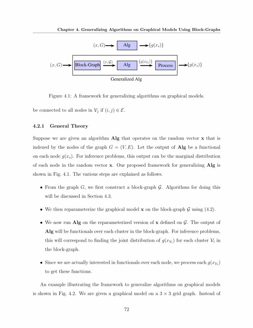
Chapter 4. Generalizing Algorithms on Graphical Models Using Block-Graphs
Alg(x,G) g(xs)
Algg(xVi
)Block-Graph
(x,G)Process(x,G) g(xs)
Generalized Alg
Figure 4.1: A framework for generalizing algorithms on graphical models.
be connected to all nodes in Vj if (i, j) ∈ E .
4.2.1 General Theory
Suppose we are given an algorithm Alg that operates on the random vector x that is
indexed by the nodes of the graph G = (V,E). Let the output of Alg be a functional
on each node g(xs). For inference problems, this output can be the marginal distribution
of each node in the random vector x. Our proposed framework for generalizing Alg is
shown in Fig. 4.1. The various steps are explained as follows.
• From the graph G, we first construct a block-graph G. Algorithms for doing this
will be discussed in Section 4.3.
• We then reparameterize the graphical model x on the block-graph G using (4.2).
• We now run Alg on the reparameterized version of x defined on G. The output of
Alg will be functionals over each cluster in the block-graph. For inference problems,
this will correspond to finding the joint distribution of g(xVi) for each cluster Vi in
the block-graph.
• Since we are actually interested in functionals over each node, we process each g(xVi)
to get these functions.
An example illustrating the framework to generalize algorithms on graphical models
is shown in Fig. 4.2. We are given a graphical model on a 3 × 3 grid graph. Instead of
72
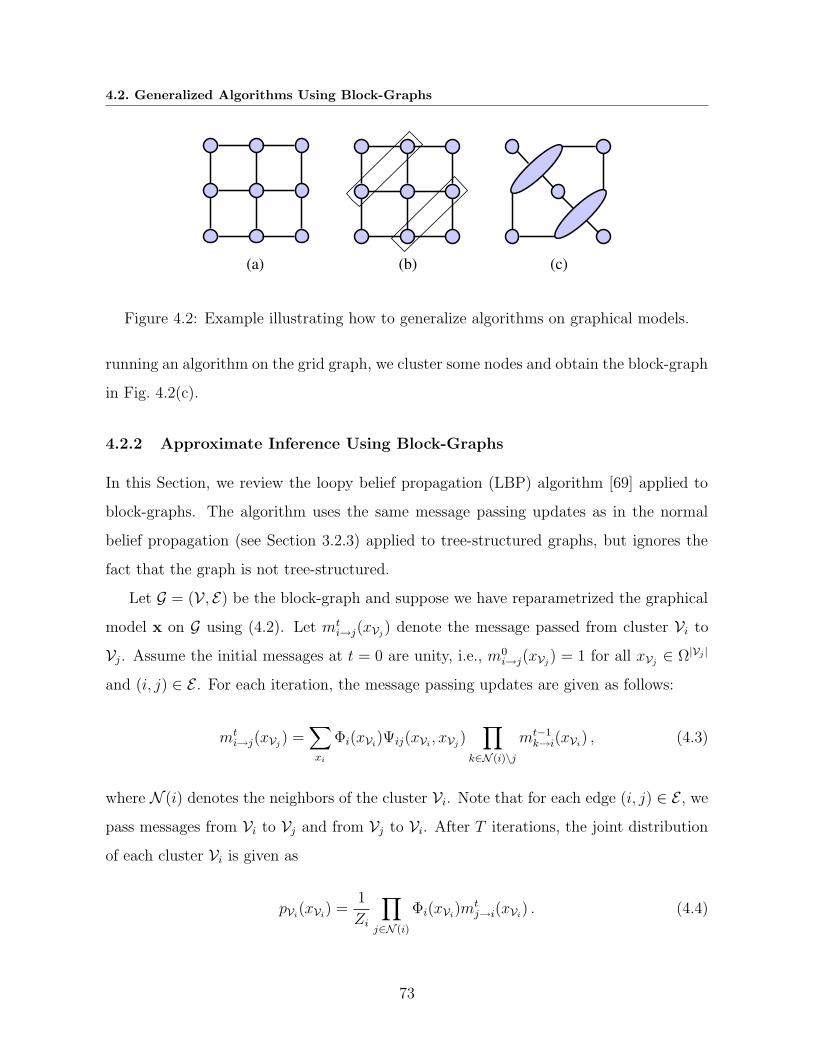
4.2. Generalized Algorithms Using Block-Graphs
(a) (b) (c)
Figure 4.2: Example illustrating how to generalize algorithms on graphical models.
running an algorithm on the grid graph, we cluster some nodes and obtain the block-graph
in Fig. 4.2(c).
4.2.2 Approximate Inference Using Block-Graphs
In this Section, we review the loopy belief propagation (LBP) algorithm [69] applied to
block-graphs. The algorithm uses the same message passing updates as in the normal
belief propagation (see Section 3.2.3) applied to tree-structured graphs, but ignores the
fact that the graph is not tree-structured.
Let G = (V , E) be the block-graph and suppose we have reparametrized the graphical
model x on G using (4.2). Let mti→j(xVj
) denote the message passed from cluster Vi to
Vj. Assume the initial messages at t = 0 are unity, i.e., m0i→j(xVj
) = 1 for all xVj∈ Ω|Vj |
and (i, j) ∈ E . For each iteration, the message passing updates are given as follows:
mti→j(xVj
) =∑
xi
Φi(xVi)Ψij(xVi
, xVj)∏
k∈N (i)\j
mt−1k→i(xVi
) , (4.3)
where N (i) denotes the neighbors of the cluster Vi. Note that for each edge (i, j) ∈ E , we
pass messages from Vi to Vj and from Vj to Vi. After T iterations, the joint distribution
of each cluster Vi is given as
pVi(xVi
) =1
Zi
∏
j∈N (i)
Φi(xVi)mt
j→i(xVi) . (4.4)
73
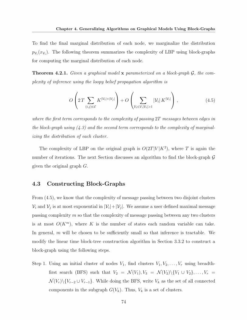
Chapter 4. Generalizing Algorithms on Graphical Models Using Block-Graphs
To find the final marginal distribution of each node, we marginalize the distribution
pVi(xVi
). The following theorem summarizes the complexity of LBP using block-graphs
for computing the marginal distribution of each node.
Theorem 4.2.1. Given a graphical model x parameterized on a block-graph G, the com-
plexity of inference using the loopy belief propagation algorithm is
O
2T
∑
(i,j)∈E
K |Vi|+|Vj |
+O
∑
Vi∈V,|Vi|>1
|Vi|K|Vi|
, (4.5)
where the first term corresponds to the complexity of passing 2T messages between edges in
the block-graph using (4.3) and the second term corresponds to the complexity of marginal-
izing the distribution of each cluster.
The complexity of LBP on the original graph is O(2T |V |K2), where T is again the
number of iterations. The next Section discusses an algorithm to find the block-graph G
given the original graph G.
4.3 Constructing Block-Graphs
From (4.5), we know that the complexity of message passing between two disjoint clusters
Vi and Vj is at most exponential in |Vi|+ |Vj|. We assume a user defined maximal message
passing complexity m so that the complexity of message passing between any two clusters
is at most O(Km), where K is the number of states each random variable can take.
In general, m will be chosen to be sufficiently small so that inference is tractable. We
modify the linear time block-tree construction algorithm in Section 3.3.2 to construct a
block-graph using the following steps.
Step 1. Using an initial cluster of nodes V1, find clusters V1, V2, . . . , Vr using breadth-
first search (BFS) such that V2 = N (V1), V3 = N (V2)\V1 ∪ V2, . . . , Vr =
N (Vr)\Vr−2 ∪ Vr−1. While doing the BFS, write Vk as the set of all connected
components in the subgraph G(Vk). Thus, Vk is a set of clusters.
74
4.3. Constructing Block-Graphs
Step 2. To ensure that the user defined maximal message passing complexity is satisfied,
for k odd, we split the clusters in Vk so that each cluster has maximal cardinality
dm/2e and for k even, we split clusters in Vk so that each cluster has maximal
cardinality bm/2c. This ensures that for all messages passed between clusters in
different Vk, the message passing complexity is at most O(Km).
Step 3. For Vr, if there exists any cluster that has cardinality greater than dm/2e or
bm/2c, depending on whether r is odd or even, partition those components. Let
Vr = V 1r , V
2r , . . . , V
mrr be the final set clusters.
Step 4. We perform the next steps for each k = r − 1, r − 2, . . . , 1, starting at k = r − 1.
Let Vk be the set of all clusters Vk that have cardinality greater than dm/2e or
bm/2c, dependending on whether k is odd or even.
Step 5. Partition all clusters in Vk into appropriate size clusters of size dm/2e or bm/2c
and also ensuring that the message passing complexity between clusters created
is at most O(Km).
Step 6. We now merge the clusters in the set Vk\Vk. The idea used in merging clusters
is that if two clusters are connected to the same cluster in Vk+1, then by merging
these two clusters, we reduce one edge in the final block-graph. Further, if two
clusters in Vk are not connected to the same cluster in Vk+1, we do not merge
these two clusters, since the number of edges in the final block-graph will remain
the same. The final clusters constructed using the above rules are denoted as
Vk = V 1k , . . . , V
mk
k .
Step 7. The block-graph is given by the clusters V =r⋃
k=1
V 1k , V
2k , . . . , V
mk
k and the set of
edges E between clusters.
The key step in the above algorithm is Step 6, where we cluster nodes appropriately.
Fig. 4.3 explains the intuition behind merging clusters with an example. Suppose, we use
the block-graph construction algorithm up to Step 5 and now we want to merge clusters
75
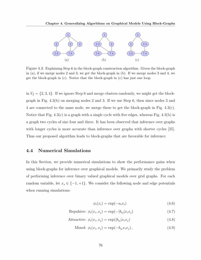
Chapter 4. Generalizing Algorithms on Graphical Models Using Block-Graphs
1
2 3 4
5 6 7 8
(a)
1
42 3
5 6 7 8
(b)
1
2 3 4
5 6 7 8
(c)
Figure 4.3: Explaining Step 6 in the block-graph construction algorithm. Given the block-graph
in (a), if we merge nodes 2 and 3, we get the block-graph in (b). If we merge nodes 3 and 4, we
get the block-graph in (c). Notice that the block-graph in (c) has just one loop.
in V2 = 2, 3, 4. If we ignore Step 6 and merge clusters randomly, we might get the block-
graph in Fig. 4.3(b) on merging nodes 2 and 3. If we use Step 6, then since nodes 3 and
4 are connected to the same node, we merge these to get the block-graph in Fig. 4.3(c).
Notice that Fig. 4.3(c) is a graph with a single cycle with five edges, whereas Fig. 4.3(b) is
a graph two cycles of size four and three. It has been observed that inference over graphs
with longer cycles is more accurate than inference over graphs with shorter cycles [25].
Thus our proposed algorithm leads to block-graphs that are favorable for inference.
4.4 Numerical Simulations
In this Section, we provide numerical simulations to show the performance gains when
using block-graphs for inference over graphical models. We primarily study the problem
of performing inference over binary valued graphical models over grid graphs. For each
random variable, let xs ∈ −1,+1. We consider the following node and edge potentials
when running simulations:
φi(xi) = exp(−aixi) (4.6)
Repulsive: φi(xi, xj) = exp(−|bij|xixj) (4.7)
Attractive: φi(xi, xj) = exp(|bij|xixj) (4.8)
Mixed: φi(xi, xj) = exp(−bijxixj) , (4.9)
76

4.4. Numerical Simulations
where ai ∼ N (0, (0.252) and bij ∼ N (0, 1). For distributions with attractive (repulsive)
potentials, neighboring random variables are more likely to take the same (opposite) value.
For distributions with mixed potentials, some neighbors are attractive, whereas some are
repulsive. We consider three types of graphs: 7 × 7 grid graphs, 8 × 8 grid graphs, and
30 × 30 grid graphs. The analysis of the results from the numerical simulations are as
follows:
• Notation: LBP refers to running loopy belief propagation on the original graph.
LBPm refers to running LBP on a block-graph constructed using our proposed al-
gorithm in Section 4.3 such that the maximal message passing complexity is O(Km).
LBPm-Rand refers to using a modification of the algorithm in Section 4.3 so that
instead of merging clusters in a structured manner using Step 5 and Step 6, we
instead merge clusters randomly. Note that each iteration of the LBP algorithm
has complexity O(2|E|K2). On the other hand, running LBP on block-graphs has
higher complexity (see Theorem 4.5). To objectively compare results on the number
of iterations, we rescale the values. Thus, if the LBP on a block-graph converges
in T iterations, we rescale this number by T · C ′/C, where C ′ is the complexity of
inference using the block-graph and C is the complexity of using just the graph.
We declare convergence if the absolute difference between the messages passed in
successive iterations is less than a threshold of ε = 10−4. If the algorithm does not
converge in 3000 iterations, we say the algorithm failed to converge. Given the true
marginal distribution ps(xs) of each node and an estimate ps(xs), the accuracy is
measured by
Accuracy =1
2|V |
∑
xs∈−1,+1
|ps(xs)− ps(xs)| . (4.10)
• 7×7 grid graph: Fig. 4.4 shows results of running LBP on block-graphs and running
LBP on the original 7 × 7 grid graph. The first three columns report the number
of times the algorithm converged out of 500 runs. LBP using mixed potentials
converged only 60% of the time, whereas LBP4 and LBP4-Rand converged on all
77
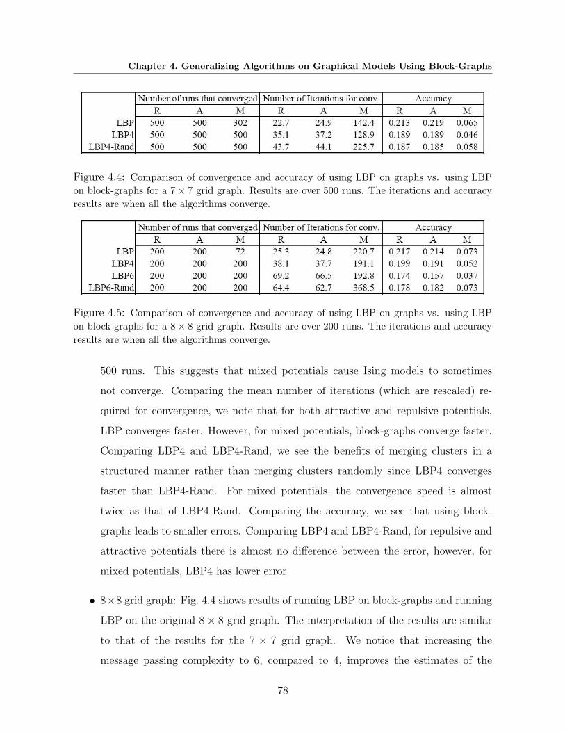
Chapter 4. Generalizing Algorithms on Graphical Models Using Block-Graphs
Figure 4.4: Comparison of convergence and accuracy of using LBP on graphs vs. using LBP
on block-graphs for a 7× 7 grid graph. Results are over 500 runs. The iterations and accuracy
results are when all the algorithms converge.
Figure 4.5: Comparison of convergence and accuracy of using LBP on graphs vs. using LBP
on block-graphs for a 8× 8 grid graph. Results are over 200 runs. The iterations and accuracy
results are when all the algorithms converge.
500 runs. This suggests that mixed potentials cause Ising models to sometimes
not converge. Comparing the mean number of iterations (which are rescaled) re-
quired for convergence, we note that for both attractive and repulsive potentials,
LBP converges faster. However, for mixed potentials, block-graphs converge faster.
Comparing LBP4 and LBP4-Rand, we see the benefits of merging clusters in a
structured manner rather than merging clusters randomly since LBP4 converges
faster than LBP4-Rand. For mixed potentials, the convergence speed is almost
twice as that of LBP4-Rand. Comparing the accuracy, we see that using block-
graphs leads to smaller errors. Comparing LBP4 and LBP4-Rand, for repulsive and
attractive potentials there is almost no difference between the error, however, for
mixed potentials, LBP4 has lower error.
• 8×8 grid graph: Fig. 4.4 shows results of running LBP on block-graphs and running
LBP on the original 8× 8 grid graph. The interpretation of the results are similar
to that of the results for the 7 × 7 grid graph. We notice that increasing the
message passing complexity to 6, compared to 4, improves the estimates of the
78

4.5. Related Work
node potentials at the cost of higher computational cost. Comparing LBP6-Rand
to LBP4, we notice that for mixed potentials LBP4 performs better suggesting and
LBP6-Rand performs as good as LBP.
• 30 × 30 grid graph: Fig. 4.4 shows results of running LBP on block-graphs and
running LBP on the original 30 × 30 grid graph. In this case, over 100 runs, the
LBP failed to converge in 3000 iterations. The interpretation of the results is the
same as before. We note that to compare the quality of the estimates, we did
not have the true estimates available since it is computationally intractable to find
these since the graph has high treewidth. Instead we ran LBP on a block-graph
with maximal message passing complexity O(K10) and used these estimates as the
ground truth. Note that even though LBP did not get converge in 3000 iterations,
the quality of the estimate is almost the same as that of using LBP8-Rand.
From the numerical simulations presented above, it is clear that using LBP on block-
graphs leads to more accurate estimates of the marginal distributions. For repulsive
and attractive node potentials, we observed that higher accuracy comes at the cost of
more computations. For mixed potentials, we observed that using block-graphs was more
accurate and faster than using the original graph. Further, we evaluated our proposed
algorithm for constructing block-graphs and noticed that our proposed algorithm leads to
more accurate estimates when compared to an approach of randomly selecting clusters.
This shows the advantage of using the block-tree as an initial estimate of the block-graph.
4.5 Related Work
There has been a lot of work in extending the BP algorithm of message passing between
nodes to message passing between clusters. It is known that the true marginal distri-
butions of a graphical model minimizes the Gibbs free energy [35]. In [114], [115], the
authors showed that the fixed points of the BP algorithm minimize the Bethe free energy,
which is an approximation to the Gibbs free energy. This motivated the Generalized Be-
79
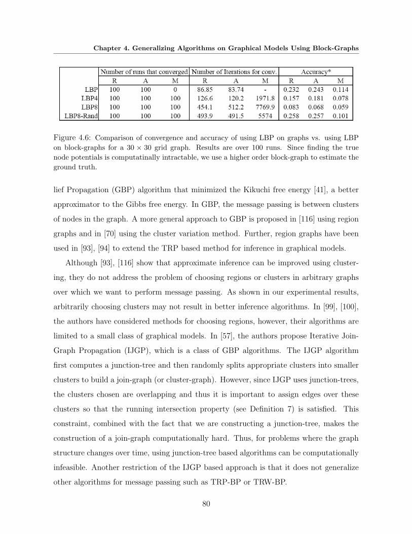
Chapter 4. Generalizing Algorithms on Graphical Models Using Block-Graphs
Figure 4.6: Comparison of convergence and accuracy of using LBP on graphs vs. using LBP
on block-graphs for a 30 × 30 grid graph. Results are over 100 runs. Since finding the true
node potentials is computatinally intractable, we use a higher order block-graph to estimate the
ground truth.
lief Propagation (GBP) algorithm that minimized the Kikuchi free energy [41], a better
approximator to the Gibbs free energy. In GBP, the message passing is between clusters
of nodes in the graph. A more general approach to GBP is proposed in [116] using region
graphs and in [70] using the cluster variation method. Further, region graphs have been
used in [93], [94] to extend the TRP based method for inference in graphical models.
Although [93], [116] show that approximate inference can be improved using cluster-
ing, they do not address the problem of choosing regions or clusters in arbitrary graphs
over which we want to perform message passing. As shown in our experimental results,
arbitrarily choosing clusters may not result in better inference algorithms. In [99], [100],
the authors have considered methods for choosing regions, however, their algorithms are
limited to a small class of graphical models. In [57], the authors propose Iterative Join-
Graph Propagation (IJGP), which is a class of GBP algorithms. The IJGP algorithm
first computes a junction-tree and then randomly splits appropriate clusters into smaller
clusters to build a join-graph (or cluster-graph). However, since IJGP uses junction-trees,
the clusters chosen are overlapping and thus it is important to assign edges over these
clusters so that the running intersection property (see Definition 7) is satisfied. This
constraint, combined with the fact that we are constructing a junction-tree, makes the
construction of a join-graph computationally hard. Thus, for problems where the graph
structure changes over time, using junction-tree based algorithms can be computationally
infeasible. Another restriction of the IJGP based approach is that it does not generalize
other algorithms for message passing such as TRP-BP or TRW-BP.
80
4.6. Summary
Our proposed approach of using non-overlapping clusters for approximate inference
has been considered before. In the original paper describing GBP [114], the authors gave
an example of how disjoint clusters can be used, however, there have been no algorithms
in the literature that show how such clusters can be chosen. In [111], [112], the au-
thors use disjoint clusters to generalize mean field algorithms for approximate inference.
Although we don’t demonstrate the use of our algorithm for mean field methods, the clus-
tering algorithm used in [112] is based on standard graph partitioning algorithms that are
computationally intensive for large graphs. Our approach to forming clusters is simple,
efficient, and motivated by observations that inference over graphs with longer cycles is
easier than inference over graphs with shorter cycles.
4.6 Summary
We proposed a framework for generalizing algorithms over graphical models using the
notion of block-graphs, defined as a graph where each node is a cluster of nodes and
the clusters are disjoint. We proposed a simple and efficient algorithm for constructing
block-graphs that relied on block-trees to construct an initial estimate of the disjoint
cluster of nodes. Our numerical simulations showed the advantages of using block-graphs
for approximate inference over graphical models. We also showed that our proposed
algorithm for constructing block-graphs leads to more accurate estimates of marginal
distributions than an algorithm that randomly selects clusters to form a block-graph.
81

Chapter 4. Generalizing Algorithms on Graphical Models Using Block-Graphs
82

Chapter 5
Conclusion and Future Work
5.1 List of Contributions
In this thesis, we studied the problem of finding tree-structured like representations for
Markov random fields (MRFs). Our main contributions are as follows:
1. For MRFs over continuous indices, we showed that tree-structured like represen-
tations can be derived over a collection of hypersurfaces. This reparameterization
of the field allowed us to study MRFs as Markov processes, thereby allowing us to
extend algorithms like the Kalman-Bucy filter to random fields.
2. For MRFs over graphs, we showed that tree-structured like representations can be
derived by clustering nodes in the original graph to construct a tree-structured graph
over the cluster of nodes. We called the resulting tree over the clusters a block-
tree and showed how the belief propagation algorithm for inference (computing
marginal distribution given a joint distribution) over MRFs can be extended to
MRFs characterized by block-trees.
3. Finally, we proposed an algorithm for generalizing various algorithms over graphical
models using the notion of a block-graph, defined as a graph over disjoint cluster of
nodes. We proposed an efficient algorithm for constructing block-graphs and showed
how our framework for generalization can be used for generalized belief propagation.
83

Chapter 5. Conclusion and Future Work
Collection of hypersurfaces
1 2 3
4 65
7 8 9
Collection of clusters
Figure 5.1: An example of the tree-structures we derive in this thesis. For MRFs over continuous
indices, we derive tree representations over hypersurfaces. For MRFs over graphs, we derive tree
representations over a disjoint collection of clusters over nodes.
5.2 Chapter Summaries
5.2.1 Chapter 2: Tree-Structures in MRFs over Continuous Indices
In Chapter 2, we derived tree-structured like representations for MRFs indexed over
continuous indices. Although these MRFs were introduced in 1956 by Levy, there had
been no prior work on finding recursive representations that can enable the extension of
Kalman filters to random fields. We showed that a natural tree like representation for
MRFs exists on a collection of hypersurfaces starting at the boundary and telescoping
inwards. See Fig. 5.1 for an example for an example.
To derive recursive representations, we parameterized the field indexed over some
region S ∈ Rd, d > 1, by a tuple (λ, θ), where λ ∈ [0, 1] is the parameter over which
we derive recursions and θ ∈ Θ ⊂ Rd−1 parameterizes the hypersurfaces over which we
define recursions. For Gaussian MRFs (GMRFs), we showed that a representation over
the hypersurfaces is given by a linear stochastic differential equation of the form
dxλ(θ) = Fθ[xλ(θ)] +Bλ(θ)wλ(θ) , (5.1)
where Fθ[xλ(θ)] is a functional over the field defined on xλ(θ) for all θ ∈ Θ and the driv-
ing noise wλ(θ) can be interpreted as Brownian motion for each fixed θ. Equation (5.1)
84

5.2. Chapter Summaries
generalizes known state-space models for Gaussian Markov random processes to GMRFs.
Using (5.1), we derived extensions of the Kalman-Bucy filter [40] and Rauch-Tung-Striebel
smoother [75]. The recursions for the Kalman filter initiated at the boundary and tele-
scoped inwards and the recursions for the smoother telescoped inwards and outwards.
5.2.2 Chapter 3: Block-Tree Structures in MRFs over Graphs
In Chapter 3, we studied MRFs indexed over graphs, often referred to as graphical models.
Our main contribution was to show that a tree-structured representation for arbitrary
graphical models can be derived by clustering nodes in the graph to form a tree over
disjoint clusters of nodes. Our proposed algorithm for constructing such graphs, which
we call block-trees, is simple and efficient with a complexity linear in the number of edges.
See Fig. 5.1 for an example of a block-tree for a 3× 3 grid graph.
We compared block-trees to junction-trees [77], a tree-structured graph over clusters
that are overlapping. We showed that constructing block-trees is faster than constructing
junction-trees. Further, in the context of inference over graphical models (computing
marginal distributions given a joint probability distribution), we showed the advantages of
using block-trees vs. using junction-trees. Finally, we proposed an algorithm for choosing
between a junction-tree and a block-tree when performing inference over graphical models.
5.2.3 Chapter 4: Generalizing Algorithms on Graphical Models
In Chapter 4, we proposed a framework for generalizing algorithms over graphical models.
The main idea is to cluster nodes in the graph to form a block-graph and then run algo-
rithms over the block-graph instead of the original graph. As an example, we showed how
loopy belief propagation (LBP) [69], an approximate inference algorithm for computing
marginal distributions, can be easily generalized using block-graphs. The need for ap-
proximate inference algorithm arises because for many graphs, the clusters in a block-tree
or a junction-tree can be large, so performing exact inference is intractable.
Our main contribution is to propose an algorithm for constructing block-graphs that
85

Chapter 5. Conclusion and Future Work
modifies the algorithm for constructing block-trees. The main idea is to split larger
clusters in a block-tree so that there are minimal number of edges in the block-graph.
Numerically, we observed that using LBP on block-graphs leads to better estimates than
using LBP on the original graph. Further, we also observed that using our proposed
algorithm for constructing block-graphs leads to better estimates than using a block-
graph constructed by randomly clustering nodes.
5.3 Suggestions for Future Work
The work in this thesis naturally leads to other research ideas that we briefly discuss here.
5.3.1 Estimation of Random Fields Over Continuous Indices
In this thesis, we showed that a natural recursive representation for Markov random fields
(MRFs) is in terms of tree-structured like representations over a collection of hypersur-
faces. In reality, a random field may not necessarily be an MRF. For such cases, it is
of interest to find efficient algorithms for processing data. To do this, we can study the
problem of finding an approximate telescoping representation given an arbitrary Gaus-
sian random field. Further, since there is flexibility in choosing the hypersurfaces in
the telescoping representation, there can exist multiple different approximate telescop-
ing representations. Thus, one way to proceed is to model the underlying random field
as a mixture of telescoping representations on various collections of hypersurfaces. This
approach to finding stochastic models is in concept similar to work done in [60], where
the authors model an arbitrary distribution using a mixture of tree-structured graphical
models.
5.3.2 Other Applications of Using Block-Graphs
In this thesis, we proposed a framework for generalizing current algorithms on graphical
models. As an example, we consider the problem of generalizing loopy belief propagation
and showed numerical simulations to validate that the generalized algorithm leads to bet-
86
5.3. Suggestions for Future Work
ter estimates. It is easy to see that other known algorithms can also be generalized. It will
be interesting to see what kinds of improvements one can get by running the generalized
algorithm on other algorithms. Further, our approach to generalizing algorithms is not
only limited to inference algorithms, but can also be applied to problems such as MAP
inference [96] and computing the partition function for graphical models [95].
5.3.3 Learning Graphical Models Using Block-Graphs
In this thesis, we considered the problem of deriving algorithms on graphical models.
Another problem of interest in graphical models is to derive algorithms for learning the
structure and parameters of a graphical models given observed samples. This problem
in general is NP-hard, however, there are works in the literature [61], [76] that propose
consistent algorithms for learning graphical models under some conditions. In recent
work, we have derived theoretical conditions under which algorithms for learning graphi-
cal models can be improved [91] using ideas from list decoding [22]. We have also applied
the idea of clustering nodes towards a problem on approximating high-dimensional dis-
tributions [20]. One interesting question that can be asked is whether graphical model
selection algorithms can be improved if we cluster nodes and apply current algorithms
for learning graphical model to the cluster of nodes instead of individual nodes them-
selves. This approach can be thought of as the extension of the generalized algorithm we
proposed in Chapter 4.
87

Chapter 5. Conclusion and Future Work
88
Appendix A
Appendix to Chapter 2
A.1 Computing bj(s, r) in Theorem 2.2.1
We show how the coefficients bj(s, r) are computed for a GMRF x(t), t ∈ T ⊂ Rd. Let
G− and G+ be complementary sets in T ⊂ Rd as shown in Fig. 2.2. Following [73], define
a function hs(t) such that
hs(t) =
R(s, t) t ∈ G− ∪ ∂G
hs(t) : Lths(t) = 0 ,
hs(∂G) = R(s, ∂G) t ∈ G+
hs(t) ∈ Hm0 (T )
, (A.1)
where Lr is defined in (2.11) and Hm0 (T ) is the completion of C∞
0 (T ), the set of infinitely
differentiable function with compact support in T , under the norm Sobolov norm order
m. From (2.10), it is clear that hs(r) 6= R(s, r) when r ∈ G+. Let u(r) ∈ C∞0 (T ) and
consider the following steps for computing bj(s, r):
∑
|α|,|β|≤m
∫
T
Dαu(t)aαβ(t)Dβhs(t)dt
=∑
|α|,|β|≤m
∫
G−
Dαu(t)aα,β(t)DβR(s, t)dr∑
|α|,|β|≤m
∫
G+
Dαu(t)aα,β(t)Dβhs(t)dr (A.2)
89
Chapter A. Appendix to Chapter 2
=m−1∑
j=0
∫
∂G
bj(s, r)∂j
∂nju(r)dl +
∫
G−
u(r)LtR(s, t)dt+
∫
G+
u(t)Lths(t)dt (A.3)
=m−1∑
j=0
∫
∂G
bj(s, r)∂j
∂nju(r)dl . (A.4)
To get (A.2), we split the integral integral on the left hand side over G− and G+. In
going from (A.2) to (A.3), we use integration by parts and the fact that u(r) ∈ C∞0 (T ).
We get (A.4) using (2.10) and (A.1). Thus, to compute bj(s, r), we first need to find hs(r)
using (A.1) and then use the steps in (A.2)−(A.4). We now present an example where
we compute bj(s, r) for a Gauss-Markov process.
Example: Let x(t) ∈ R be the Brownian bridge on T = [0, 1] such that
x(t) = w(t)− tw(1) , (A.5)
where w(t) is a standard Brownian motion. Since covariance of w(t) is min(t, s), the
covariance of x(t) is given by
R(t, s) =
s(1− t) t > s
t(1− s) t < s. (A.6)
Using the theory of reciprocal processes, see [46], [52], it can be shown that the operator
Lt is
LtR(t, s) = −∂2R(t, s)
∂t2= δ(t− s) . (A.7)
Thus, the inner product associated with R(t, s) is given by
< u, v >= 〈Du,Dv〉T =
∫ 1
0
∂
∂su(s)
∂
∂sv(s)ds . (A.8)
Following (A.1), for r < 1 and s ∈ [r, 1], hs(t) = R(s, t) for t ∈ [0, r] and
−∂2
∂t2hs(t) = 0 , t > r (A.9)
90

A.1. Computing bj(s, r) in Theorem 2.2.1
hs(r) = r(1− s) , hs(1) = 0 . (A.10)
We can trivially show that hs(t) is given by
hs(t) =r(1− s)
1− r(1− t) , t ≥ r . (A.11)
We now follow the steps in (A.2)-(A.4):
∫ 1
0
∂
∂tu(t)
∂
∂ths(t)dt =
∫ r
0
∂
∂tu(t)
∂
∂tR(s, t)dt+
∫ 1
r
∂
∂tu(t)
∂
∂ths(t)dt
= u(t)∂
∂tR(s, t)
∣∣∣∣r
0
+ u(t)∂
∂ths(t)
∣∣∣∣1
r
=
(∂
∂tR(s, r)−
∂
∂rhs(r)
)u(r) .
=1− s
1− ru(r) .
Using Theorem 2.2.1, we can compute E[x(s)|σx(t) : 0 ≤ t ≤ r] as
E[x(s)|σx(t) : 0 ≤ t ≤ r] = E[x(s)|x(r)] =
(1− s
1− r
)x(r) . (A.12)
We note that since x(t) is a Gauss-Markov process, it is known that, [107],
E[x(s)|x(r)] = R(s, r)R−1(r, r)x(r) . (A.13)
Using the expression for R(s, r), we can easily verify that (A.12) and (A.13) are equivalent.
91
Chapter A. Appendix to Chapter 2
A.2 Proof of Theorem 2.3.1: Telescoping Representation
Let xλ+dλ|λ(θ) denote the conditional expectation of xλ+dλ(θ) given the σ-algebra gener-
ated by the field xµ(α) : (µ, α) ∈ [0, λ]×Θ. From Theorem 2.2.1, we have
xλ+dλ|λ(θ) =m−1∑
j=0
∫
Θ
bj((λ+ dλ, θ), (λ, α))dj
dnjxλ(α)dα . (A.14)
It is clear that xλ(θ) = xλ|λ(θ). Taking the limit in (A.14) as dλ→ 0, we have
xλ(θ) =m−1∑
j=0
∫
Θ
bj((λ, θ), (λ, α))dj
dnjxλ(α)dα . (A.15)
Define the error as ξλ+dλ(θ) such that
ξλ+dλ(θ) = xλ+dλ(θ)− xλ+dλ(θ) . (A.16)
Adding and subtracting xλ(θ) in (A.16) and using (A.15), we have
xλ+dλ(θ)− xλ(θ) =m−1∑
j=0
∫
Θ
[bj((λ+ dλ, θ), (λ, α))
− bj((λ, θ), (λ, α))]dj
dnjxλ(α)dα + ξλ+dλ(θ) . (A.17)
Assuming dλ is small, we can write bj((λ+ dλ, θ), (λ, α))− bj((λ, θ), (λ, α)) as
bj((λ+ dλ, θ), (λ, α))− bj((λ, θ), (λ, α))
=bj((λ+ dλ, θ), (λ, α))− bj((λ, θ), (λ, α))
dλdλ (A.18)
=
(lim
µ→λ+
∂
∂µbj((µ, θ), (λ, α))
)dλ , (A.19)
where in going from (A.18) to (A.19), we use the assumption that dλ is close to zero.
92

A.2. Proof of Theorem 2.3.1: Telescoping Representation
Writing dxλ(θ) = xλ+dλ(θ)− xλ(θ) and substituting (A.19) in (A.17), we get
dxλ(θ) = Fθ[xλ(θ)]dλ+ ξλ+dλ(θ) , (A.20)
where Fθ is given in (2.18). To get the final form of the telescoping representation, we
need to characterize ξλ+dλ(θ). To do this, we write ξλ+dλ(θ) as
ξλ+dλ(θ) = Bλ(θ)dwλ(θ) = Bλ(θ)[wλ+dλ(θ)− wλ(θ)] . (A.21)
We now prove the properties of wλ(θ):
i) Since ξλ(θ) = xλ(θ)− xλ|λ(θ) and xλ|λ(θ) = xλ(θ) by definition, we have
limdλ→0
ξλ+dλ(θ) = ξλ(θ) = 0 , a.s. .
Thus, using (A.21), since Bλ(θ) 6= 0, we have
limdλ→0
wλ+dλ(θ)− wλ(θ) = 0, a.s. (A.22)
limdλ→0
wλ+dλ(θ) = wλ(θ), a.s. (A.23)
Equation (A.23) shows that wλ(θ) is almost surely continuous in λ.
ii) Since the driving noise at the boundary of the field can be captured in the boundary
conditions, without loss in generality, we can assume that w0(θ) = 0 for all θ ∈ Θ.
iii) For 0 ≤ λ1 ≤ λ′1 ≤ λ2 ≤ λ′2 and θ1, θ2 ∈ Θ, let dλ1 = λ′1 − λ1 and dλ2 = λ′2 − λ2.
Consider the covariance
E[ξλ1+dλ1(θ1)ξλ2+dλ2
(θ2] = E [(xλ1+dλ1(θ1)− xλ1+dλ1
(θ1)) ξλ2+dλ2(θ2)] (A.24)
= E[xλ1+dλ1(θ1)ξλ2+dλ2
(θ2)] (A.25)
− E[xλ1+dλ1(θ1)ξλ2+dλ2
(θ2)]
= 0 , (A.26)
93
Chapter A. Appendix to Chapter 2
where to go from (A.24) to (A.25), we use the orthogonality of the error. Using the
definition of ξλ+dλ(θ) in (A.21), we have that wλ′1(θ1)−wλ1
(θ1) and wλ′2(θ2)−wλ2
(θ2)
are independent random variables.
iv) We now compute E[ξλ+dλ(θ1)ξλ+dλ(θ2)]:
E[ξλ+dλ(θ1)ξλ+dλ(θ2)]
= E[ξλ+dλ(θ1)(xλ+dλ(θ2)− xλ+dλ|λ(θ2))]
= E[(xλ+dλ(θ1)− xλ+dλ|λ(θ1))xλ+dλ(θ2)]
= Rλ+dλ,λ+dλ(θ1, θ2)−m−1∑
j=0
∫
Θ
bj((λ+ dλ, θ1), (λ, α))∂j
∂njRλ,λ+dλ(α, θ2)dα
= Rλ+dλ,λ+dλ(θ1, θ2)−Rλ,λ+dλ(θ1, θ2) +Rλ,λ+dλ(θ1, θ2) (A.27)
−m−1∑
j=0
∫
Θ
bj((λ+ dλ, θ1), (λ, α))∂j
∂njRλ,λ+dλ(α, θ2)dα .
Using (A.15), we have
Rλ,λ+dλ(θ1, θ2) = E[xλ(θ1)xλ+dλ(θ2)] (A.28)
=m−1∑
j=0
∫
Θ
bj((λ, θ1), (λ, α))∂j
∂njRλ,λ+dλ(α, θ2)dα . (A.29)
Substituting (A.29) in (A.27), we have
E[ξλ+dλ(θ1)ξλ+dλ(θ2)]
= Rλ+dλ,λ+dλ(θ1, θ2)−Rλ,λ+dλ(θ1, θ2)−m−1∑
j=0
∫
Θ
[bj((λ+ dλ, θ1), (λ, α)) (A.30)
− bj((λ, θ1), (λ, α))]∂j
∂njRλ,λ+dλ(α, θ2)dα
=
[Rλ+dλ,λ+dλ(θ1, θ2)−Rλ,λ+dλ(θ1, θ2)
dλ
]dλ
−
[m∑
j=0
∫
Θ
(bj((λ+ dλ, θ1), (λ, α))− bj((λ, θ1), (λ, α))
dλ
)∂j
∂njRλ,λ+dλ(α, θ2)dα
]dλ
94

A.2. Proof of Theorem 2.3.1: Telescoping Representation
=
(lim
µ→λ−
∂
∂µRµ,λ(θ1, θ2)− lim
µ→λ+
∂
∂µ
m−1∑
j=0
∫
Θ
bjµ,λ(θ1, α)∂j
∂njRλ,λ(α, θ2)dα
)dλ
=
(lim
µ→λ−
∂
∂µRµ,λ(θ1, θ2)− lim
µ→λ+
∂
∂µRµ,λ(θ1, θ2)
)dλ
= Cλ(θ1, θ2)dλ . (A.31)
Thus, for dλ small, we have
E [(wλ+dλ(θ1)− wλ(θ1))(wλ+dλ(θ2)− wλ(θ2))] =Cλ(θ1, θ2)
Bλ(θ1)Bλ(θ2)dλ . (A.32)
Since w0(θ) = 0, we can use (A.32) to compute E[wλ(θ1)wλ(θ2)] as follows:
E[(wλ(θ1)− w0(θ1))(wλ(θ2)− w0(θ2))]
= limN→∞
E
[N+1∑
k=0
(wγk(θ1)− wγk−1
(θ2))N+1∑
k=0
(wγk(θ2)− wγk−1
(θ2))
], γ0 = λ, γN+1 = 0
(A.33)
= limN→∞
E
[N+1∑
k=0
(wγk(θ1)− wγk−1
(θ1))(wγk(θ2)− wγk−1
(θ2))
](A.34)
= limN→∞
N+1∑
k=0
Cγk−1(θ1, θ2)
Bγk−1(θ1)Bγk−1(θ2)
(γk − γk−1) (A.35)
=
∫ λ
0
Cu(θ1, θ2)
Bu(θ1)Bu(θ2)du . (A.36)
We get (A.34) using the orthogonal increments property in (iii). We use (A.32) to get
(A.35). We use the definition of the Riemann integrals to go from (A.35) to (A.36).
v) For λ1 > λ2, the covariance of wλ1(θ)− wλ2
(θ) is computed as follows:
E[(wλ1(θ)− wλ2
(θ))2] = E[w2λ1
(θ)] + E[w2λ2
(θ)]− 2E[wλ1(θ)wλ2
(θ)] (A.37)
95

Chapter A. Appendix to Chapter 2
= λ1 + λ2 − 2
∫ λ2
0
Cu(θ1, θ2)
Bu(θ1)Bu(θ2)du , (A.38)
where
E[w2λ(θ)] =
∫ λ
0
Cu(θ, θ)
B2u(θ)
du (A.39)
=
∫
u∈[0,λ]:Cu(θ,θ)=0
Cu(θ, θ)
B2u(θ)
du+
∫
u∈[0,λ]:Cu(θ,θ)6=0
Cu(θ, θ)
B2u(θ)
du (A.40)
=
∫
u∈[0,λ]:Cu(θ,θ)6=0
du (A.41)
= λ . (A.42)
To go from (A.40) to (A.41), we use (2.17) since Cu(θ, θ) 6= 0. To go from (A.41)
to (A.42), we use the given assumption that the set u ∈ [0, 1] : Cu(θ, θ) = 0 has
measure zero.
A.3 Proof of Theorem 2.6.1: Recursive Filter
The steps involved in deriving the recursive filter are the same as deriving the Kalman-
Bucy filtering equations, see [68]. The only difference is that we need to take into account
the dependence of each point in the random field on its neighboring telescoping surface
(which is captured in the integral transform Fθ), instead of a neighboring point as we do
for Gauss-Markov processes. The steps in deriving the recursive filter are summarized as
follows. In Step 1, we define the innovation process and show that it is Brownian motion
and equivalent to the observation space. Using this, we find a relationship between the
filtered estimate and the innovation, see Lemma A.3.1. In Step 2, we find a representation
for the field xλ(θ), see Lemma A.3.4. Using Lemma A.3.1 and Lemma A.3.4, we find a
closed form expression for xλ|λ(θ) in Step 3. We differentiate this to derive the equation
for the filtered estimate in Step 4. Finally, Step 5 computes the equation for the error
covariance.
96
A.3. Proof of Theorem 2.6.1: Recursive Filter
Step 1. [Innovations] Define qλ(θ) such that
qλ(θ) = yλ(θ)−
∫ λ
0
Gµ(θ)xµ|µ(θ)dµ .
Define the innovation field eλ(θ) such that
deλ(θ) =1
Dλ(θ)dvλ(θ) (A.43)
=Gλ(θ)
Dλ(θ)xλ|λ(θ)dλ+ dnλ(θ) , (A.44)
where we have used (2.53) to get the final expression in (A.44) and assume thatDλ(θ) 6= 0.
Lemma A.3.1. The field eλ(θ) is Brownian motion for each fixed θ and E[eλ1(θ1)eλ2
(θ2)] =
0 when λ1 6= λ2, θ1 6= θ2.
Proof. Note that E[xλ|λ(θ)|σeµ(θ) : 0 ≤ µ ≤ λ] = 0 since xλ|λ(θ) ⊥ yµ(α) for α ∈ Θ,
0 ≤ µ ≤ λ. Thus, using Corollary 8.4.5 in [68], we establish that eλ(θ) is Brownian motion
for each fixed θ. Assume λ1 > λ2 and consider γ < λ2. Then, using the orthogonality of
error, xµ(θ1) ⊥ yγ(α) for γ < µ, and the fact that nλ(θ) ⊥ eγ(α) for γ < λ, we have
E[(eλ1(θ1)− eλ2
(θ2))eγ(α)] =
∫ λ1
λ2
(Gµ(θ)
Dµ(θ)
)E[xµ|µ(θ1)eγ(α)]dµ
+ E[(nλ1(θ1)− nλ2
(θ1))eγ(α)] (A.45)
= 0 . (A.46)
Now we compute E[deλ1(θ1)deλ2
(θ2)] for λ1 > λ2:
E[deλ1(α1)deλ2
(θ2)] = E
[(Gλ1
(α1)
Dλ1(θ1)
xλ1|λ1(θ1)dλ1 + dnλ1
(θ1)
)deλ2
(θ2)
](A.47)
= E[dnλ1(θ1)deλ2
(θ2)] (A.48)
=1
Dλ2(θ2)
E[dnλ1
(θ1)(dyλ2
(θ2)−Gλ2(θ2)xλ2|λ2
(θ2)dλ2
)](A.49)
97

Chapter A. Appendix to Chapter 2
=1
Dλ2(θ2)
E[dnλ1(θ1)dyλ2
(θ2)] (A.50)
=1
Dλ2(θ2)
E[dnλ1(θ1) (Gλ2
(θ2)xλ2(θ2)dθ2 +Dλ2
(θ2)dnλ2(θ2))]
(A.51)
= E[dnλ1(θ1)dnλ2
(θ2)] = 0 . (A.52)
To go from (A.47) to (A.48), we use that xλ1|λ1(θ1) is independent of deλ2
(θ2), since
deλ2(θ2) is a linear combination on the observations y(∂T s), s ∈ [0, λ2]. We get (A.49)
using the definition of deλ2(θ2) in (A.44). To go from (A.49) to (A.50), we use that
dnµ1(θ1) is independent of xλ2|λ2
(θ2) for λ1 > λ2. We get (A.51) using the equation for
the observations in (2.53). To go from (A.51) to (A.52), we use the assumption that
nλ1(θ1) is independent of the GMRF xλ(θ). In a similar manner, we can get the result
for λ1 < λ2.
For λ1 6= λ2 and θ1 6= θ2, E[eλ1(θ1)eλ2
(θ2)] = 0 follows from similar computations as
done in (A.33)−(A.36).
Lemma A.3.1 says that the innovation has the properties as the noise observation
nλ(θ). We now use the innovation to find a closed form expression for the filtered estimate
xλ|λ(θ).
Lemma A.3.2. The filtered estimate xλ|λ(θ) can be written in terms of the innovation as
xλ|λ(θ) =
∫ λ
0
∫
Θ
gλ,µ(θ, α)deµ(α)dα (A.53)
gλ,µ(θ, α) =∂
∂µE[xλ(θ)eµ(α)] . (A.54)
Proof. Using the methods in [68] or [37], we can establish the equivalence between the
innovations and the observations. Because of this equivalence, we can write the filtered
estimate as in (A.53). We now compute gλ,µ(θ, α). We know that
(xλ(θ)− xλ|λ(θ)
)⊥ eµ(α) , µ ≤ λ, α ∈ Θ .
98

A.3. Proof of Theorem 2.6.1: Recursive Filter
Thus, we have
E[xλ(θ)eµ(α)] = E[xλ|λ(θ)eµ(α)] (A.55)
=
∫ λ
0
∫
Θ
gλ,s(θ, β)E[des(β)eµ(α)]dβ (A.56)
=
∫ λ
0
∫
Θ
∫ µ
0
gλ,s(θ, β)E[des(β)der(α)]dβ (A.57)
=
∫ λ
0
∫ µ
0
∫
Θ
gλ,s(θ, β)δ(s− r)δ(β − α)dsdrdβ (A.58)
=
∫ µ
0
gλ,r(θ, α)dr . (A.59)
To go from (A.57) to (A.58), we use Lemma A.3.1. Differentiating (A.59) with respect to
µ, we get the expression for gλ,µ(θ, α) in (A.54).
Step 2. [Formula for xλ(θ)] Before deriving a closed form expression for xλ(θ), we first
need the following Lemma.
Lemma A.3.3. For any function Ψλ,γ(θ1, θ2) with m− 1 normal derivatives, we have
∫ λ
0
Fθ1[Ψλ,γ(θ1, θ2)]dγ = Fθ1
[∫ λ
0
Ψλ,γ(θ1, θ2)dγ
]. (A.60)
Proof. Using the definition of Fθ1, we have
∫ λ
0Fθ1
[Ψλ,γ(θ1, θ2)]dγ
=
∫ λ
0
m−1∑
j=0
∫
Θ
limµ→λ+
∂
∂µbj((µ, θ), (λ, α)) lim
h→0
∂j
∂hjΨλ+hλ,γ(α + hα, θ2)dαdγ (A.61)
=m−1∑
j=0
∫
Θ
limµ→λ+
∂
∂µbj((µ, θ), (λ, α)) lim
h→0
∂j
∂hj
[∫ λ
0
Ψλ+hλ,γ(α+ hα, θ2)dγ
]dα (A.62)
= Fθ1
[∫ λ
0
Ψλ,γ(θ1, θ2)dγ
]. (A.63)
99

Chapter A. Appendix to Chapter 2
Lemma A.3.4. Using the telescoping representation for xλ(θ), a solution for xλ(θ) is
given as follows:
xλ(θ) =
∫
Θ
Φλ,µ(θ, α)xµ(α)dα +
∫
Θ
∫ λ
µ
Φλ,γ(θ, α)dwγ(α)dα , (A.64)
∂
∂λΦλ,µ(θ, α) = Fθ [Φλ,µ(θ, α)] ,Φλ,λ = δ(θ − α) .
Proof. We show that (A.64) satisfies the differential equation in (2.47). Taking derivative
of (A.64) with respect to λ, we have
dxλ(θ) =
∫
Θ
∂
dλΦλ,µ(θ, α)xµ(α)dαdλ+
∫
Θ
Φλ,λ(θ, α)dwλ(α) +
∫
Θ
∫ λ
µ
∂
dλΦλ,γ(θ, α)dwγ(α)dα
(A.65)
=
∫
Θ
Fθ [Φλ,µ(θ, α)] xµ(α)dαdλ+ dwλ(θ) +
∫
Θ
∫ λ
µ
Fθ [Φλ,γ(θ, α)] dwγ(α)dα
(A.66)
= Fθ
[∫
Θ
Φλ,µ(θ, α)xµ(α)dα +
∫
Θ
∫ λ
µ
Φλ,γ(θ, α)dbγ(α)dα
]+ dwλ(θ) (A.67)
= Fθ[xλ(θ)] + dwλ(θ) . (A.68)
To get (A.67), we use Theorem A.3.3 to take the integral transform Fθ outside the integral.
Since the xλ(θ) in (A.64) satisfies (2.47), it must be a solution.
Step 3. [Equation for xλ|λ(θ)] Using (A.44) and (A.64), we can write gλ,µ(θ, α) in
(A.54) as
gλ,µ(θ, α) =∂
∂µE
xλ(θ)
[∫ µ
0
Gγ(α)
Dγ(α)xγ|γ(α)dγ + nµ(α)
](A.69)
=∂
∂µ
[∫ u
0
Gγ(α)
Dγ(α)E[xλ(θ)xγ|γ(α)]dγ
](A.70)
=∂
∂µ
∫ u
0
Gγ(α)
Dγ(α)
∫
Θ
Φλ,γ(θ, β)E[xγ(β)xγ|γ(α)]dβdγ
(A.71)
100

A.3. Proof of Theorem 2.6.1: Recursive Filter
=Gµ(α)
Dµ(α)
∫
Θ
Φλ,µ(θ, β)E[xµ(β)xµ|µ(α)]dβ (A.72)
=Gµ(α)
Dµ(α)
∫
Θ
Φλ,µ(θ, β)Sµ(β, α)dβ . (A.73)
To get (A.73), we use the fact that xµ|µ(α) ⊥ xµ|µ(β), so that
E[xµ(β)xµ|µ(α)] = E[xµ|µ(β)xµ|µ(α)] = Sµ(β, α) .
Substituting (A.73) in the expression for xλ|λ(θ) in (A.54) (Step 2), we get
xλ|λ(θ) =
∫ λ
0
∫
Θ
Gµ(α)
Dµ(α)
[∫
Θ
Φλ,µ(θ, β)Sµ(β, α)dβ
]deµ(α)dα . (A.74)
Step 4. [Differential Equation for xλ|λ(θ)] Differentiating (A.74) with respect to λ,
we get
dxλ|λ(θ) =
∫
Θ
Gλ(α)
Dλ(α)Sµ(θ, α)deλ(α)dα (A.75)
+
∫ λ
0
∫
Θ
Gµ(α)
Dµ(α)
[∫
Θ
Fθ[Φλ,µ(θ, β)]Sµ(β, α)dβ
]deµ(α)dα
=
∫
Θ
Gλ(α)
Dλ(α)Sλ(α, θ)deλ(α)dα + Fθ[xλ|λ(θ)]dλ (A.76)
= Fθ[xλ|λ(θ)]dλ+Kθ[deλ(θ)] , (A.77)
where Kθ is the integral transform defined as in (2.60).
Step 5. [Differential Equation for Sλ(α, θ)] The error covariance Sλ(α, θ) can be
written as
Sλ(α, θ) = E[xλ|λ(α)xλ|λ(θ)] (A.78)
= E[xλ(α)xλ(θ)]− E[xλ|λ(α)xλ|λ(θ)] . (A.79)
101
Chapter A. Appendix to Chapter 2
Using expressions for xλ(α) in (A.64), we can show that for Pλ(α, β) = E[xλ(α)xλ(θ)],
∂Pλ(α, θ)
dλ= Fα[Pλ(α, θ)] + FθPλ(α, θ) + Cλ(α, θ) . (A.80)
Using the expression for xλ|λ(α) in (A.53), it can be shown that
∂E[xλ|λ(α)xλ|λ(θ)]
dλ= Fα[E[xλ|λ(α)xλ|λ(θ)]] + Fθ[E[xλ|λ(α)xλ|λ(θ)]] (A.81)
+
∫
Θ
G2λ(β)
D2λ(β)
Sλ(α, β)Sλ(θ, β)dβ .
Differentiating (A.79) and using (A.80) and (A.81), we get the desired equation:
∂
∂λSλ(α, θ) = Fα[Sλ(α, θ)] + Fθ[Sλ(α, θ)] + Cλ(θ, α)−
∫
Θ
G2λ(β)
D2λ(β)
Sλ(α, β)Sλ(θ, β)dβ .
(A.82)
A.4 Proof of Theorem 2.6.2: Recursive Smoother
We now derive smoothing equations. Using similar steps as in Lemma A.3.2, we can show
that
xλ|T (θ) =
∫ 1
0
∫
Θ
gλ,µ(θ, α)deµ(α)dα , (A.83)
gλ,µ(θ, α) =∂
∂µE[xλ(θ)eµ(α)] . (A.84)
Define the error covariance Sλ,µ(θ, α) as
Sλ,µ(θ, α) = E[xλ|λ(θ)xµ|µ(α)] . (A.85)
We have the following result for the smoother:
Lemma A.4.1. The smoothed estimator xλ|T (θ) is given by
xλ|T (θ) = xλ|λ(θ) +
∫ 1
λ
∫
Θ
gλ,µ(θ, α)deµ(α)dα , (A.86)
102

A.4. Proof of Theorem 2.6.2: Recursive Smoother
where for µ ≥ λ,
gλ,µ(θ, α) =Gµ(α)
Dµ(α)Sλ,µ(θ, α) . (A.87)
Proof. Equation (A.86) immediately follows from (A.83) and Lemma A.3.2. Equation
(A.87) follows by using (A.44) to compute gλ,µ(θ, α) in (A.84).
We now want to characterize the error covariance Sλ,µ(θ, α). Subtracting the tele-
scoping representation in (2.47) and the filtering equation in (2.58), we get the following
equation for the filtering error covariance:
dxµ|µ(α) = Fθ[xµ|µ(α)]dµ+Bµ(α)dwµ(α)−Kα[dnµ(α)] , (A.88)
where Fα is the integral transform
Fα[xµ|µ(α)] = Fα[xµ|µ(α)]−Kα
[Gµ(α)
Dµ(α)xµ|µ(α)
]. (A.89)
Just like we did in Lemma A.3.4, we can write a solution to (A.88) as
xµ|µ(α) =
∫
Θ
Φµ,λ(α, θ)xλ|λ(θ)dθ +
∫
Θ
∫ µ
λ
Φµ,γ(α, θ)[Bγ(θ)dwγ(θ)−Kθ[dnγ(θ)]]dθ
(A.90)
∂
∂µΦµ,λ(α, θ) = FαΦµ,λ(α, θ) and Φµ,µ(α, θ) = δ(α− θ) . (A.91)
Differentiating (A.90) with respect to λ, we can show that
∫
Θ
∂
∂λΦµ,λ(α, β)xλ|λ(β)dβ=−
∫
Θ
Φµ,λ(α, β)Fβxλ|λ(β)dβ . (A.92)
Substituting (A.90) in (A.88), we have the following relationship:
Sλ,µ(θ, α) =
∫
Θ
Φµ,λ(α, β)Sλ(β, θ)dβ . (A.93)
103

Chapter A. Appendix to Chapter 2
Substituting (A.93) in (A.86) and (A.87), differentiating (A.86) and using (A.92) and
(2.61), we get the following equation:
dxλ|T (θ) = Fθ[xλ|T (θ)]dλ+
∫ 1
λ
∫
Θ
Gu(α)
Du(α)
∫
Θ
Φµ,λ(α, β)Cλ(β, θ)dβdeµ(α)dα . (A.94)
Assuming Sλ(θ, θ) > 0, we get smoother equations using the following calculations:
dxλ|T (β)δ(θ − β) = Fβ[xλ|T (β)]δ(θ − β)dλ+
∫ 1
λ
∫
Θ
Gu(α)
Du(α)Φµ,λ(α, β)Cλ(β, θ)deµ(α)dα
(A.95)
Sλ(β, θ)
Cλ(β, θ)dxλ|T (β)δ(θ − β) =
Sλ(β, θ)
Cλ(β, θ)Fβ[xλ|T (β)]δ(θ − β)dλ
+
∫ 1
λ
∫
Θ
Gu(α)
Du(α)Φµ,λ(α, β)Sλ(β, θ)deµ(α)dα (A.96)
Sλ(θ, θ)
Cλ(θ, θ)dxλ|T (θ) =
Sλ(θ, θ)
Cλ(θ, θ)Fθ[xλ|T (θ)]dλ
+
∫ 1
λ
∫
Θ
Gu(α)
Du(α)
(∫
Θ
Φµ,λ(α, β)Sλ(β, θ)dβ
)deµ(α)dα
(A.97)
dxλ|T (θ) = Fθ[xλ|T (θ)]dλ+Cλ(θ, θ)
Sλ(θ, θ)
∫ 1
λ
∫
Θ
Gu(α)
Du(α)Sλ,µ(θ, α)deµ(α)dα
(A.98)
dxλ|T (θ) = Fθ[xλ|T (θ)]dλ+Cλ(θ, θ)
Sλ(θ, θ)[xλ|T (θ)− xλ|λ(θ)] . (A.99)
Equation (A.94) is equivalent to (A.95). We multiply (A.95) by Sλ(β, θ)/Cλ(β, θ) to get
(A.96). We integrate (A.96) for all β to get (A.97). To go from (A.97) to (A.98), we use
(A.93). Equation (A.98) follows from (A.86).
To derive a differential equation for Sλ|T (α, θ), we first note that
Sλ|T (α, θ) = E[xλ|T (α)xλ|T (θ)] (A.100)
= E[xλ(α)xλ(θ)]− E[xλ|T (α)xλ|T (θ)] . (A.101)
104

A.4. Proof of Theorem 2.6.2: Recursive Smoother
Using (A.86) to compute E[xλ|T (α)xλ|T (θ)], we can find an expression for Sλ|T (α, θ) as
Sλ|T (α, θ) = Sλ(α, θ)−
∫ 1
λ
∫
Θ
G2µ(α)
D2µ(α)
Sµ,λ(α1, α)Sµ,λ(α1, θ)dµdα1 . (A.102)
Taking derivative of (A.102), we get (2.68).
105

Chapter A. Appendix to Chapter 2
106

Bibliography
[1] M. B. Adams, A. S. Willsky, and B. C. Levy. Linear estimation of boundary value
stochastic processes – Part I: The role and construction of complimentary models.
IEEE Trans. Autom. Control, AC–29(9):803–811, September 1984.
[2] M. B. Adams, A. S. Willsky, and B. C. Levy. Linear estimation of boundary value
stochastic processes – Part II: 1-D smoothing problems. IEEE Trans. Autom. Con-
trol, AC–29(9):811–821, September 1984.
[3] A. Anandkumar, V. Tan, and A. Willsky. High dimensional structure learning of
Ising models on sparse random graphs. arXiv:1011.0129v6 [math.ST], 2011.
[4] A. Anandkumar, J. Yukich, L. Tong, and A. Willsky. Detection Error Exponent for
Spatially Dependent Samples in Random Networks. In Proc. of IEEE ISIT, Seoul,
S. Korea, July 2009.
[5] S. Arnborg, D. G. Corneil, and A. Proskurowski. Complexity of finding embeddings
in a k-tree. SIAM J. Algebraic Discrete Methods, 8(2):277–284, 1987.
[6] F. Badawi, A. Lindquist, and M. Pavon. A stochastic realization approach to the
smoothing problem. IEEE Trans. Autom. Control, AC-24:878–888, 1979.
[7] A. Bagchi and H. Westdijk. Smoothing and likelihood ratio for Gaussian boundary
value processes. IEEE Trans. Autom. Control, 34(9):954–962, September 1989.
107
BIBLIOGRAPHY
[8] A. Becker and D. Geiger. A sufficiently fast algorithm for finding close to optimal
junction trees. In Proceedings of the 10th Annual Conference on Uncertainty in
Artificial Intelligence (UAI-96), pages 81–89, 1996.
[9] S. Bernstein. Sur les liaisons entre les grandeurs aleatoires. Proc. Int. Cong. of
Math., pages 288–309, 1932.
[10] A. Berry, P. Heggernes, and G. Simonet. The minimum degree heuristic and the
minimal triangulation process. In H. Bodlaender, editor, Graph-Theoretic Concepts
in Computer Science, volume 2880 of Lecture Notes in Computer Science, pages
58–70. Springer Berlin / Heidelberg, 2003.
[11] J. Besag. Spatial interaction and the statistical analysis of lattice systems. Journal
of the Royal Statistical Society. Series B (Methodological), 36(2):192–236, 1974.
[12] H. L. Bodlaender and A. M. Koster. Treewidth computations I. upper bounds.
Information and Computation, 208(3):259 – 275, 2010.
[13] W. S. Burdic. Underwater Acoustic System Analysis. Englewood Cliffs, NJ: Prentice
Hall, 1984.
[14] Z. Chaczko and F. Ahmad. Wireless sensor network based system for fire endan-
gered areas. In Proceedings of the Third International Conference on Information
Technology and Applications (ICITA’05) Volume 2 - Volume 02, ICITA ’05, pages
203–207, Washington, DC, USA, 2005. IEEE Computer Society.
[15] V. Chandrasekaran, N. Srebro, and P. Harsha. Complexity of inference in graph-
ical models. In Proceedings of the Proceedings of the Twenty-Fourth Conference
Annual Conference on Uncertainty in Artificial Intelligence (UAI-08), pages 70–78,
Corvallis, Oregon, 2008. AUAI Press.
[16] F. M. Coetzee and V. L. Stonick. On a natural homotopy between linear and
nonlinear single layer networks. IEEE Trans. Neural Networks, 7:307–317, 1994.
108
BIBLIOGRAPHY
[17] G. F. Cooper. NESTOR: A computer-based medical diagnostic aid that integrates
causal and probabilistic knowledge. PhD thesis, Department of Computer Science,
Stanford University, 1984.
[18] G. F. Cooper. The computational complexity of probabilistic inference using
Bayesian belief networks (research note). Artificial Intelligence, 42(2-3):393–405,
1990.
[19] F. G. Cozman. Generalizing variable elimination in Bayesian networks. In Workshop
on Probabilistic Reasoning in Artificial Intelligence, pages 27–32, 2000.
[20] U. S. J. M. F. M. D. Vats, Vishal Monga. Scalable robust hypothesis tests using
graphical models. In Proc. International Conference on Acoustics, Speech, and
Signal Processing ICASSP, Mar. 14–19, 2011.
[21] R. Dechter. Bucket elimination: A unifying framework for reasoning. Artificial
Intelligence, 113(1-2):41–85, Sep 1999.
[22] P. Elias. List decoding for noisy channels. Wescon Convention Record, pages 94–107,
1957.
[23] P. Erdos and A. Renyi. On the evolution of random graphs. In Publication of the
Mathematical Institute of the Hungarian Academy of Sciences, pages 17–61, 1960.
[24] P. Erdos and A. Renyi. On random graphs. I. Publ. Math. Debrecen, 6:290–297,
1959.
[25] E. Fabre and A. Guyader. Dealing with short cycles in graphical codes. In IEEE
International Symposium on Information Theory (ISIT), Sorrento, June 2000.
[26] A. Ferrante and G. Picci. Minimal realization and dynamic properties of optimal
smoothers. IEEE Trans. Autom. Control, 45:2028–2046, 2000.
[27] N. Friedman. Inferring Cellular Networks Using Probabilistic Graphical Models.
Science, 303(5659):799–805, 2004.
109

BIBLIOGRAPHY
[28] R. G. Gallagar. Low-density parity check codes. IRE Trans. Inform. Theory.,
IT-8:21–28, 1962.
[29] E. N. Gilbert. Random graphs. The Annals of Mathematics Statistics, 30(4):1141–
1144, 1959.
[30] A. Ihler, S. Kirshner, M. Ghil, A. Robertson, and P. Smyth. Graphical models
for statistical inference and data assimilation. Physica D: Nonlinear Phenomena,
230:72–87, June 2007.
[31] M. O. Jackson. Social and Economic Networks. Princeton University Press, 2008.
[32] B. Jamison. Reciprocal processes: The stationary Gaussian case. The Annals of
Mathematical Statistics, 41:1624–1630, 1970.
[33] F. Jensen and F. Jensen. Optimal junction trees. In Proceedings of the 10th Annual
Conference on Uncertainty in Artificial Intelligence (UAI-94), pages 360–36, San
Francisco, CA, 1994. Morgan Kaufmann.
[34] F. V. Jenson, S. L. Lauritzen, and K. G. Oleson. Bayesian updating in causal
probabilistic networks by local computation. Computational Statistics Quarterly,
4:269–282, 1990.
[35] M. Jordan, Z. Ghahramani, T. Jaakkola, and L. Saul. An introduction to variational
methods for graphical models. Machine Learning, 37:183–233, 1999.
[36] P. R. Julian and A. Cline. The direct estimation of spatial wavenumber spectra of
atmospheric variables. J. Atmospheric Sci., 31:1526–1539, 1974.
[37] T. Kailath, A. H. Sayed, and B. Hassibi. Linear Estimation. Prentice Hall, 2000.
[38] Kallianpur and Mandrekar. The Markov property for generalized Gaussian random
fields. Ann. Inst. Fourier, 24:143–167, 1974.
110

BIBLIOGRAPHY
[39] R. E. Kalman. A new approach to linear filtering and prediction problems. Trans-
actions of the ASME–Journal of Basic Engineering, 82(Series D):35–45, 1960.
[40] R. E. Kalman and R. Bucy. New results in linear filtering and prediction the-
ory. Transactions of the ASME–Journal of Basic Engineering, 83(Series D):95–108,
1960.
[41] R. Kikuchi. A theory of cooperative phenomena. Phys. Rev., 81(6):988– 988–1003,
1951.
[42] U. B. Kjaerulff. Triangulation of graphs - algorithms giving small total state space.
Technical Report Research Report R-90-09, Department of Mathematics and Com-
puter Science, Aalborg University, Denmark, 1990.
[43] A. J. Krener. Reciprocal processes and the stochastic realization problem for acausal
systems. In C. I. Byrnes and A. Lindquist, editors, Modelling, Identification, and
Robust Control, pages 197–209. Amsterdam: Elsevier, 1986.
[44] A. J. Krener. Realizations of reciprocal processes. Stochastics and Stochastics
Reports, 34:29–56, 1988.
[45] A. J. Krener. Reciprocal diffusions and stochastic differential equations of second
order. Stochastics, 24:393–422, 1988.
[46] A. J. Krener, R. Frezza, and B. C. Levy. Gaussian reciprocal processes and self-
adjoint stochastic differential equations of second order. Stochastics and Stochastics
Reports, 34:29–56, 1991.
[47] J. B. Kruskal. On the shortest spanning subtree of a graph and the traveling
salesman problem. Proceedings of the American Mathematical Society, 7(1):48–50,
February 1956.
[48] S. L. Lauritzen. Graphical Models. Oxford University Press, USA, 1996.
111
BIBLIOGRAPHY
[49] S. L. Lauritzen and D. J. Spiegelhalter. Local computations with probabilities on
graphical structures and their application to expert systems. Journal of the Royal
Statistical Society. Series B (Methodological), 50(2):157–224, 1988.
[50] C. Lee, J. Lee, and S. il Oum. Rank-width of random graphs. arXiv:1001.0461v1,
2010.
[51] B. C. Levy. Characterization of multivariate stationary Gaussian reciprocal diffu-
sions. Journal of Multivariate Analysis, 62:74–79, July 1997.
[52] B. C. Levy. Principles of Signal Detection and Parameter Estimation. Springer
Verlag, 2008.
[53] B. C. Levy, M. B. Adams, and A. S. Willsky. Solution and linear estimation of 2-D
nearest-neighbor models. Proc. IEEE, 78(4):627–641, Apr. 1990.
[54] P. Levy. A special problem of Brownian motion, and a general theory of Gaussian
random functions. In Proceedings of the Third Berkeley Symposium on Mathematical
Statistics and Probability, 1954–1955, vol. II, pages 133–175, Berkeley and Los
Angeles, 1956. University of California Press.
[55] D. J. C. MacKay. Learning in Graphical Models, chapter Introduction to Monte
Carlo methods. Kluwer Academic Publishers, 1997.
[56] H. M. Markowitz. The elimination form of the inverse and its application to linear
programming. Management Science, 3(3):255–269, 1957.
[57] R. Mateescu, K. Kask, V. Gogate, and R. Dechter. Join-graph propagation algo-
rithms. Journal of Artificial Intelligence Research, 37:279–328, 2010.
[58] H. P. McKean. Brownian motion with a several dimension time. Theory of Proba-
bility and Applications, 8:335–354, 1963.
[59] C. L. Mehta and E. Wolf. Coherence properties of black body radiation, parts I and
II. Phys. Rev., 134(4):1143–1153, 1964.
112

BIBLIOGRAPHY
[60] M. Meila and M. I. Jordan. Learning with mixtures of trees. Journal of Machine
Learning Research, pages 1–48, 2000.
[61] N. Meinshausen and P. Buhlmann. High-dimensional graphs and variable selection
with the lasso. Ann. Statist., 34(3):1436–1462, 2006.
[62] J. M. F. Moura and N. Balram. Recursive structure of noncausal Gauss-Markov
random fields. IEEE Trans. Inf. Theory, IT-38(2):334–354, March 1992.
[63] J. M. F. Moura and S. Goswami. Gauss-Markov random fields (GMrf) with con-
tinuous indices. IEEE Trans. Inf. Theory, 43(5):1560–1573, September 1997.
[64] J. Munkres. Topology. Prentice Hall, 2000.
[65] J. R. Nevins, M. West, A. Dobra, A. Dobra, C. Hans, C. Hans, B. Jones, B. Jones,
J. R. Nevins, and M. W. Abstract. Sparse graphical models for exploring gene
expression data. Journal of Multivariate Analysis, 90:196–212, 2004.
[66] M. E. J. Newman, D. J. Watts, and S. H. Strogatz. Random graph models of social
networks. Proc. Natl. Acad. Sci. USA, 99:2566–2572, 2002.
[67] R. Ogier and E. Wong. Recursive linear smoothing of two-dimensional random
fields. IEEE Trans. Inf. Theory, 27(1):77–83, Jan. 1981.
[68] B. Oksendal. Stochastic Differential Equations: An Introduction with Applications
(Universitext). Springer, December 2005.
[69] J. Pearl. Probabilistic Reasoning in Intelligent Systems: Networks of Plausible In-
ference. Morgan Kaufmann, 1988.
[70] A. Pelizzola. Cluster variation method in statistical physics and probabilistic graph-
ical models. Journal of Physics A: Mathematical and General, 38(33):R309–R339,
2005.
113
BIBLIOGRAPHY
[71] Y. Peng and J. A. Reggia. Plausibility of diagnostic hypotheses. In National Con-
ference on Artificial Intelligence (AAAI’86), pages 140–145, 1986.
[72] G. Picci and F. Carli. Modelling and simulation of images by reciprocal processes.
In Tenth International Conference on Computer Modeling and Simulation, pages
513–518, Washington, DC, USA, 2008. IEEE Computer Society.
[73] L. D. Pitt. A Markov property for Gaussian processes with a multidimensional
parameter. Arch. Ration. Mech. Anal., 43:367–391, 1971.
[74] R. C. Prim. Shortest connection networks and some generalizations. Bell System
Technical Journal, 36:1389?1401, 1957.
[75] H. E. Rauch, F. Tung, and C. T. Stribel. Maximum likelihood estimates of linear
dynamical systems. AIAA J., 3(8):1445–1450, August 1965.
[76] P. Ravikumar, M. J. Wainwright, and J. Lafferty. High-dimensional Ising model
selection using `1-regularized logistic regression. Annals of Statistics, 38(3):1287–
1319, 2010.
[77] N. Robertson and P. D. Seymour. Graph minors. II. Algorithmic aspects of tree-
width. Journal of Algorithms, 7(3):309 – 322, 1986.
[78] D. J. Rose, R. E. Tarjan, and G. S. Lueker. Algorithmic aspects of vertex elimination
on graphs. SIAM Journal on Computing, 5(2):266–283, 1976.
[79] Y. A. Rozanov. Markov Random Fields. New York: Springer-Verlag, 1982.
[80] H. Rue and L. Held. Gaussian Markov Random Fields: Theory and Applications
(Monographs on Statistics and Applied Probability). Chapman & Hall/CRC, 1st
edition, February 2005.
[81] E. Schrodinger. Uber die Umkehrung der Naturgesetze. Sitzungsber. Preuss. Akad.
Wissen. Phys. Math. Kl., pages 144–153, 1931.
114
BIBLIOGRAPHY
[82] G. Shafer and P. P. Shenoy. Probability propagation. Annals of Mathematics and
Artificial Intelligence, (1-4):327–352, 1990.
[83] E. B. Sudderth, M. J. Wainwright, and A. S. Willsky. Embedded trees: estima-
tion of Gaussian processes on graphs with cycles. IEEE Trans. Signal Process.,
52(11):3136–3150, Nov. 2004.
[84] A. H. Tewfik, B. C. Levy, and A. S. Willsky. Internal models and recursive esti-
mation for 2-D isotropic random fields. IEEE Trans. Inf. Theory, 37(4):1055–1066,
July 1991.
[85] J. Theiler, G. Cao, L. R. Bachega, and C. A. Bouman. Sparse matrix transform
for hyperspectral image processing. to appear in IEEE Selected Topics in Signal
Process., 2011.
[86] E. Vanmarcke. Random Fields: Analysis and Synthesis. MIT Press, 1983.
[87] D. Vats and J. M. F. Moura. Recursive filtering and smoothing for discrete index
Gaussian reciprocal processes. In Proc. 43rd Annual Conference on Information
Sciences and Systems CISS 2009, pages 377–382, Mar. 18–20, 2009.
[88] D. Vats and J. M. F. Moura. Recursive filtering and smoothing for Gaussian re-
ciprocal processes with continuous indices. In IEEE International Symposium on
Information Theory (ISIT), Seoul, Korea, 2009.
[89] D. Vats and J. M. F. Moura. Reciprocal fields: A model for random fields pinned to
two boundaries. In Proc. IEEE International Conference on Decision and Control,
Atlanta, Dec. 2010.
[90] D. Vats and J. M. F. Moura. A telescoping approach to recursive enhancement of
noisy images. In Proc. International Conference on Acoustics, Speech, and Signal
Processing ICASSP, Mar. 14–19, 2010.
115

BIBLIOGRAPHY
[91] D. Vats and J. M. F. Moura. Necessary conditions for consistent graphical model
selection. In IEEE International Symposium on Information Theory (ISIT), Saint
Petersburg, Russia, 2011.
[92] D. Vats and J. M. F. Moura. Telescoping recursive representations and estimation
of Gauss-Markov random fields. Trans. on Information Theory, 57(3):1645 – 1663,
2011.
[93] M. J. Wainwright. Stochastic Processes on Graphs: Geometric and Variational Ap-
proaches. PhD thesis, Department of EECS, Massachusetts Institute of Technology,
2002.
[94] M. J. Wainwright, T. S. Jaakkola, and A. S. Willsky. Tree-based reparameterization
framework for analysis of sum-product and related algorithms. IEEE Trans. Inf.
Theory, 49:2003, 2003.
[95] M. J. Wainwright, T. S. Jaakkola, and A. S. Willsky. A new class of upper bounds
on the log partition function. IEEE Trans. on Information Theory, 51:2313 – 2335,
2005.
[96] M. J. Wainwright and M. I. Jordan. Graphical Models, Exponential Families, and
Variational Inference. Now Publishers Inc., Hanover, MA, USA, 2008.
[97] G. N. Watson. A Treatise on the Theory of Bessel Functions. Cambridge University
Press, second edition edition, 1995.
[98] Y. Weiss and W. T. Freeman. On the optimality of solutions of the max-product
belief propagation algorithm in arbitrary graphs. IEEE Transactions on Information
Theory, 47:723–735, 2001.
[99] M. Welling. On the choice of regions for generalized belief propagation. In Proceed-
ings of the 20th conference on Uncertainty in artificial intelligence, UAI ’04, pages
585–592, Arlington, Virginia, United States, 2004. AUAI Press.
116
BIBLIOGRAPHY
[100] M. Welling, T. Minka, and Y. W. Teh. Structured region graphs: Morphing EP into
GBP. In Proceedings of the International Conference on Uncertainty in Artificial
Intelligence, volume 21, 2005.
[101] D. B. West. Introduction to Graph Theory. Prentice Hall, 2nd edition, 2000.
[102] P. Whittle. On stationary processes in the plane. Biometrika, 41(3/4):434–449,
1954.
[103] E. Wong. Two-dimensional random fields and representation of images. SIAM
Journal on Applied Mathematics, 16(4):756–770, 1968.
[104] E. Wong. A likelihood ratio formula for two-dimensional random fields. IEEE Trans.
Inf. Theory, 20(4):418–422, July 1974.
[105] E. Wong. Recursive filtering for two-dimensional random fields (corresp.). IEEE
Trans. Inf. Theory, 21(1):84–86, Jan. 1975.
[106] E. Wong. Recursive causal linear filtering for two-dimensional random fields. IEEE
Trans. Inf. Theory, 24(1):50–59, Jan. 1978.
[107] E. Wong and B. Hajek. Stochastic Processes in Engineering Systems. Springer-
Verlag New York Inc, 1985.
[108] E. Wong and E. Tsui. One-sided recursive filters for two-dimensional random fields
(corresp.). IEEE Trans. Inf. Theory, 23(5):633–637, Sept. 1977.
[109] E. Wong and M. Zakai. Markov processes on the plane. Stochastics, 15:311–333,
1985.
[110] J. W. Woods and C. Radewan. Kalman filtering in two dimensions. IEEE Trans.
Inf. Theory, 23(4):473–482, Jul 1977.
[111] E. P. Xing, M. I. Jordan, and S. Russell. A generalized mean field algorithm for
variational inference in exponential families. In Proceedings of the 20th conference on
117

BIBLIOGRAPHY
Uncertainty in artificial intelligence, UAI ’04, pages 602–610, Arlington, Virginia,
United States, 2003. AUAI Press.
[112] E. P. Xing, M. I. Jordan, and S. Russell. Graph partition strategies for generalized
mean field inference. In Proceedings of the 20th conference on Uncertainty in artifi-
cial intelligence, UAI ’04, pages 602–610, Arlington, Virginia, United States, 2004.
AUAI Press.
[113] C. Yanover and Y. Weiss. Approximate inference and protein folding. In Advances
in Neural Information Processing Systems, pages 84–86. MIT Press, 2002.
[114] J. Yedidia, W. Freeman, and Y. Weiss. Bethe free energy, Kikuchi approximations,
and belief propagation algorithms. Technical Report TR2001-16, Mitsubishi Electric
Research Laboratories, 2001.
[115] J. S. Yedidia, W. T. Freeman, and Y. Weiss. Generalized belief propagation. In
NIPS, 2001.
[116] J. S. Yedidia, W. T. Freeman, and Y. Weiss. Constructing free energy approxima-
tions and generalized belief propagation algorithms. IEEE Transactions on Infor-
mation Theory, 51:2282–2312, 2005.
[117] N. Zhang and D. Poole. A simple approach to Bayesian network computations.
In Proceedings of the Tenth Canadian Conference on Artificial Intelligence, pages
171–178, 1994.
[118] F. Zhao, J. Peng, J. Debartolo, K. F. Freed, T. R. Sosnick, and J. Xu. A probabilistic
graphical model for ab initio folding. In Proceedings of the 13th Annual International
Conference on Research in Computational Molecular Biology, RECOMB 2’09, pages
59–73, Berlin, Heidelberg, 2009. Springer-Verlag.
118