trees and fundamental circuits - neeraj kumargraph+theory... · graph theory (ecs-505) lecture...

Graph Theory (ECS-505) Lecture Notes Trees and Fundamental Circuits

Tree A connected graph without any circuits.

o must have at least one vertex. o definition implies that it must be a simple graph. o only finite trees are being considered here.

Examples:

N3 N9

N2 … N0

N1

N

A Decision tree

Application examples:

o a family tree o a tree to represent a river and its tributaries etc. o decision trees (sorting trees) for the sorting of mail according to pin codes

Minimally connected graph A connected graph is said to be minimally connected if the removal of any one edge from it disconnects the graph.

Some Properties of Trees

Theorem 7- a. There is one and only one path between every pair of vertices in a tree. b. If in a graph G there is one and only one path between every pair of vertices, then G is a tree. c. A tree with n vertices has n — 1 edges. d. A connected graph with n vertices and n — 1 edges is a tree.

NEERAJ KUMAR, Deptt. of CSE, HCST, MATHURA 3

Graph Theory (ECS-505) Lecture Notes

e. A graph is a tree if and only if it is minimally connected. f. A graph with n vertices, n — 1 edges, and no circuits is connected. g. In any tree (with two or more vertices), there are at least two pendant vertices.

Exercise 9: Prove the seven properties (theorems 7-a to 7-g) of trees listed above.

Five equivalent definitions of a tree (derived from the set of theorems 7-a to 7-g) A graph G with n vertices is called a tree if:

1. G is connected and circuitless, or 2. G is connected and has n — 1 edges, or 3. G is circuitless and has n — 1 edges, or 4. There is exactly one path between every pair of vertices in G, or 5. G is a minimally connected graph.

Distance, Centers, Radius, and Diameter

Metric A function f(x, y) of two variables is called a metric iff:

1. f(x, y) ≥ 0, and f(x, y) = 0 iff x = y, that is, the function is non-negative, and

2. f(x, y) = f(y, x), that is, the function is symmetric, and

3. f(x, y) ≤ f(x, z) + f(z, y) for any z, that is, the function satisfies the triangle-inequality.

A function of two variables can be taken as a measure of distance between them only when the function is a metric.

Distance In a connected graph G, the distance d(vi, vj) between two of its vertices vi and vj is the length of the shortest path between them.

Theorem 8 The distance between the vertices of a connected graph is a metric.

Exercise 10 Prove the theorem 8.

Since there can be multiple paths between a pair of vertices in a connected graph in general, to get the distance we have to calculate the length of each of these paths and select the minimum as the distance. However, in a tree (a connected graph with no circuits), there is exactly one path between any pair of vertices, therefore the distance between those vertices is just the length of this only path between them.

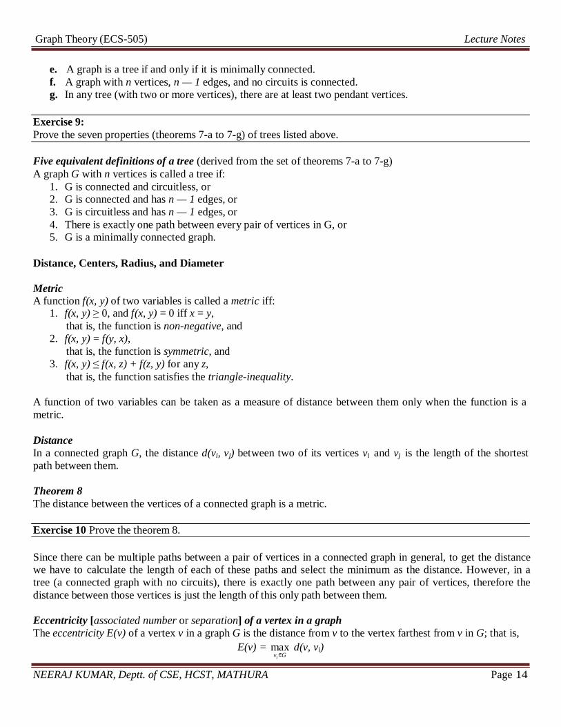
Eccentricity [associated number or separation] of a vertex in a graph The eccentricity E(v) of a vertex v in a graph G is the distance from v to the vertex farthest from v in G; that is,

E(v) = max d(v, vi) vi∈G

NEERAJ KUMAR, Deptt. of CSE, HCST, MATHURA Page 14


Center of a graph A vertex with the minimum eccentricity in a graph G is called a center of G.

A graph, in general, may have several centers.

Theorem 9 Every tree has either one or two centers.

Corollary If a tree has two centres then the two centres must be adjacent.

Diameter of a graph = Max(i, j) d(vi, vj), where vi and vj are vertices in the graph The maximum value of distance between any two vertices of the graph. Diameter = Maximum value of eccentricity in the graph.

Radius of a graph = eccentricity of the centre = minimum value of eccentricity in the graph.

Rooted and Binary Trees

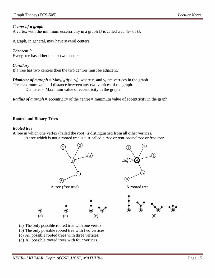
Rooted tree A tree in which one vertex (called the root) is distinguished from all other vertices. A tree which is not a rooted tree is just called a tree or non-rooted tree or free tree.

A tree (free tree) A rooted tree

(a) (b) (c) (d)

(a) The only possible rooted tree with one vertex. (b) The only possible rooted tree with two vertices. (c) All possible rooted trees with three vertices. (d) All possible rooted trees with four vertices.



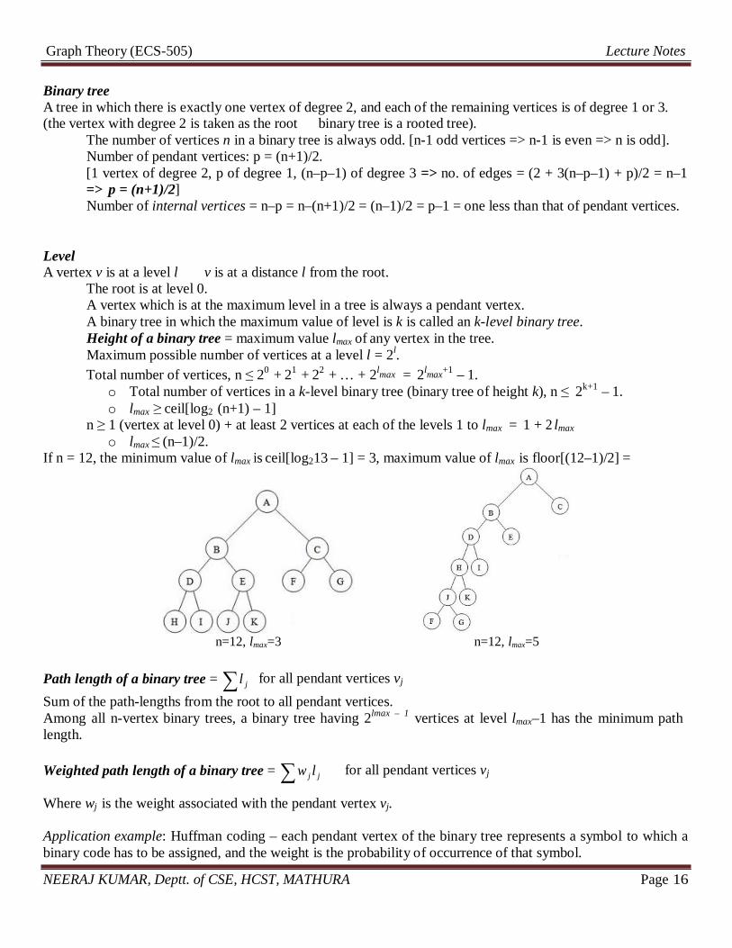
Binary tree A tree in which there is exactly one vertex of degree 2, and each of the remaining vertices is of degree 1 or 3. (the vertex with degree 2 is taken as the root binary tree is a rooted tree). The number of vertices n in a binary tree is always odd. [n-1 odd vertices => n-1 is even => n is odd]. Number of pendant vertices: p = (n+1)/2.

[1 vertex of degree 2, p of degree 1, (n–p–1) of degree 3 => no. of edges = (2 + 3(n–p–1) + p)/2 = n–1 => p = (n+1)/2]

Number of internal vertices = n–p = n–(n+1)/2 = (n–1)/2 = p–1 = one less than that of pendant vertices.

Level A vertex v is at a level l v is at a distance l from the root. The root is at level 0. A vertex which is at the maximum level in a tree is always a pendant vertex. A binary tree in which the maximum value of level is k is called an k-level binary tree. Height of a binary tree = maximum value lmax of any vertex in the tree. Maximum possible number of vertices at a level l = 2l. Total number of vertices, n ≤ 20 + 21 + 22 + … + 2lmax = 2lmax+1 – 1.

o Total number of vertices in a k-level binary tree (binary tree of height k), n ≤ 2k+1 – 1. o lmax ≥ ceil[log2 (n+1) – 1]

n ≥ 1 (vertex at level 0) + at least 2 vertices at each of the levels 1 to lmax = 1 + 2 lmax

o lmax ≤ (n–1)/2. If n = 12, the minimum value of lmax is ceil[log213 – 1] = 3, maximum value of lmax is floor[(12–1)/2] =

n=12, lmax=3 n=12, lmax=5

Path length of a binary tree = ∑ l j for all pendant vertices vj

Sum of the path-lengths from the root to all pendant vertices. Among all n-vertex binary trees, a binary tree having 2lmax – 1 vertices at level lmax–1 has the minimum path length.

Weighted path length of a binary tree = ∑ w j l j for all pendant vertices vj

Where wj is the weight associated with the pendant vertex vj.

Application example: Huffman coding – each pendant vertex of the binary tree represents a symbol to which a binary code has to be assigned, and the weight is the probability of occurrence of that symbol.



Counting the Trees

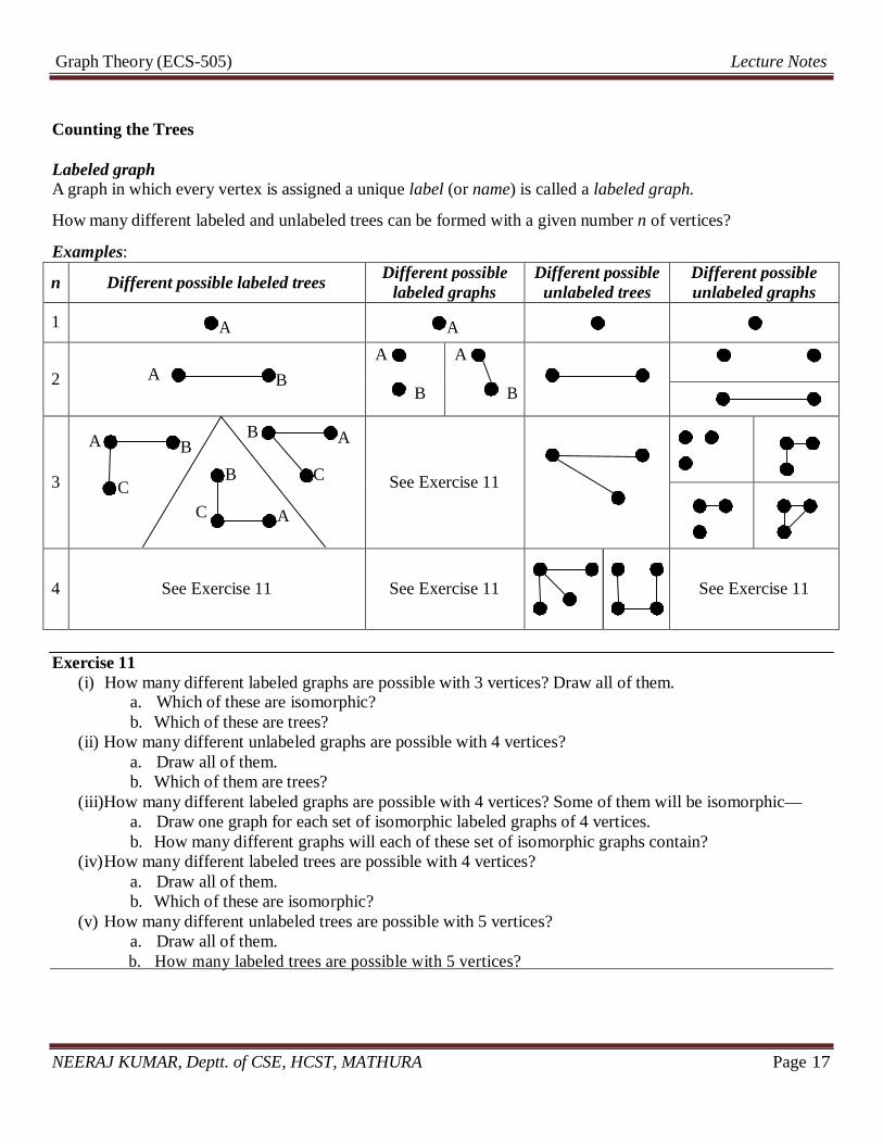
Labeled graph A graph in which every vertex is assigned a unique label (or name) is called a labeled graph.

How many different labeled and unlabeled trees can be formed with a given number n of vertices?

Examples:

n

Different possible labeled trees Different possible labeled graphs

Different possible unlabeled trees

Different possible unlabeled graphs

1

A

A

2

A B

A

B

A

B

3

A B B A

C B C

C A

See Exercise 11

4

See Exercise 11

See Exercise 11

See Exercise 11

Exercise 11

(i) How many different labeled graphs are possible with 3 vertices? Draw all of them. a. Which of these are isomorphic? b. Which of these are trees?

(ii) How many different unlabeled graphs are possible with 4 vertices? a. Draw all of them. b. Which of them are trees?

(iii)How many different labeled graphs are possible with 4 vertices? Some of them will be isomorphic— a. Draw one graph for each set of isomorphic labeled graphs of 4 vertices. b. How many different graphs will each of these set of isomorphic graphs contain?

(iv)How many different labeled trees are possible with 4 vertices? a. Draw all of them. b. Which of these are isomorphic?

(v) How many different unlabeled trees are possible with 5 vertices? a. Draw all of them.

b. How many labeled trees are possible with 5 vertices?



Theorem 10 The number of simple, labeled graphs of n vertices is: 2n (n−1)/ 2 . Proof: In a graph with n vertices and no edges, the number of distinct pairs of vertices is:

nC2 = n(n −1)/ 2 With the constraint that the graph should remain a simple graph, for every pair of vertices, we have two options—either to join them with an edge or to not join them. So, the total number of options for n(n −1)/ 2 pairs is:

2 x 2 x … n(n – 1)/2 times = 2n (n−1) / 2

So, this is also the number of simple, labeled graphs of n vertices.

Theorem 11: Cayley’s Theorem The number of labeled trees with n vertices is Tn = nn-2.

Proof: (Pitman’s ‘double-counting’ proof) Pitman's proof counts in two different ways the number of different sequences of directed edges that can be added to an empty graph on n vertices to form from it a rooted tree. One way to form such a sequence is to start with one of the Tn possible unrooted trees, choose one of its n vertices as root, and choose one of the (n − 1)! possible sequences in which to add its n − 1 edges. Therefore, the total number of sequences that can be formed in this way is Tn×n×(n − 1)! = Tn×n!.

Another way to count these edge sequences is to consider adding the edges one by one to an empty graph, and to count the number of choices available at each step. If one has added a collection of n − k edges already, so that the graph formed by these edges is a rooted forest with k trees [since, addition of every edge reduces the number of rooted trees in the forest by 1], there are n(k − 1) choices for the next edge to add: its starting vertex can be any one of the n vertices of the graph, and its ending vertex can be any one of the k roots other than the root of the tree containing the starting vertex. Therefore, if one multiplies together the number of choices from the first step, the second step, etc., the total number of choices is:

n

∏ n(k −1) = nn−1 (n −1)!= nn−2 n! k =2

Equating these two formulas for the number of edge sequences, we get: Tn×n! = nn-2×n!

and Tn = nn-2

Application example: Number of structural isomers of the saturated hydrocarbons CkH2k+2. Carbon atom (valency = 4) ↔ represent with a vertex of degree 4. Hydrogen atom (valency = 1) ↔ represent with a vertex of degree 1 (pendant vertex).

Total number of vertices = n = 3k + 2 Total number of edges = e = ½ (sum of degrees) = ½ (4k + 2k + 2)

= 3k + 1 connected graph with e = n – 1 a tree

So, the problem boils down to counting the number of different trees (labeled or unlabeled?) possible with k vertices of degree 4 and 2k+2 pendant vertices.



Spanning Tree A spanning tree [skeleton / scaffolding / maximal tree graph / maximal tree] of a connected graph G is a subgraph T of the graph G such that T is a tree and contains all the vertices of G. A tree graph is its own spanning tree.

In this connected graph, the set of edges shown in green color form a spanning tree.

Spanning forest A disconnected graph having k components has a spanning forest containing k trees, each being a spanning tree of a connected component of the graph.

In this disconnected graph with 2 components and 17 vertices, the set of edges in red color define a spanning forest containing two trees, each tree being a spanning tree of the corresponding connected component of the graph. [n=17, e=30, k=2 r = 15, µ = 15]

Algorithm to find a spanning tree of a connected graph G:

1. If G is a tree, then return G. 2. Else,

a. T=G b. while T contains a circuit

i. find a circuit in T and delete an edge from it. [T still remains connected and contains all vertices of G]

c. Return T. [T is now circuitless but connected and contains all vertices of G] Every connected graph has at least one spanning tree.

With respect to a spanning tree T of a connected graph G (or a spanning forest of a disconnected graph): An edge contained in T is called a branch. An edge not contained in T, but contained in G is called a chord [tie / link]. The complement T’ (containing all chords) of T in G is called the chord-set [tie-set / cotree] of T. If G has n vertices, e edges, and k components, then:

o Rank, r = n – k = number of branches. o Nullity, µ = e – n + k = number of chords.

Also called the cyclomatic number or first Betti number. o If G is connected, then k = 1 r = (n – 1), µ = (e – n + 1).



Fundamental Circuit A fundamental circuit of a connected graph G with respect to a spanning tree T is the circuit formed by adding a chord to T. Number of fundamental circuits in a graph = number of chords = µ Rest of the circuits in graph G are combinations of some fundamental circuits.

Cyclic Interchange [elementary tree transformation] Given a spanning tree T of a connected graph G, the process of generating another spanning tree T1 of G by adding a chord to T and deleting a branch from the fundamental circuit thus formed.

d(Ti, Tj) = Distance between two spanning trees Ti and Tj of a connected graph G having n vertices.

= number of edges which are branches of Ti but chords of Tj. = number of edges which are branches of Tj but chords of Ti. = (n – 1) – number of branches common to Ti and Tj. = (1/2) N(Ti ⊕ Tj) = (number of edges in Ti ⊕ Tj) / 2. = minimum number of cyclic interchanges needed to convert Ti to Tj (or Tj to Ti).

d(Ti, Tj) is a metric. Any spanning tree of a connected graph G can be converted into any other spanning tree of G by

successive cyclic interchanges. max

i , j

max i , j

max i , j

d (Ti ,Tj)

d (Ti ,Tj)

d (Ti ,Tj)

≤ number of branches = r ≤ number of chords = µ ≤ min (r, µ )

Central Tree A spanning tree T0 of a graph G such that:

max i

d (T0 ,Ti )

≤ max

j

d (T ,T j )

where, T is any spanning tree of G.

That is, if for each spanning tree of a graph G, the maximum among its distances to all other spanning trees of the graph is found, then central tree of G is a spanning tree for which this value is minimum among all the spanning tress of G.

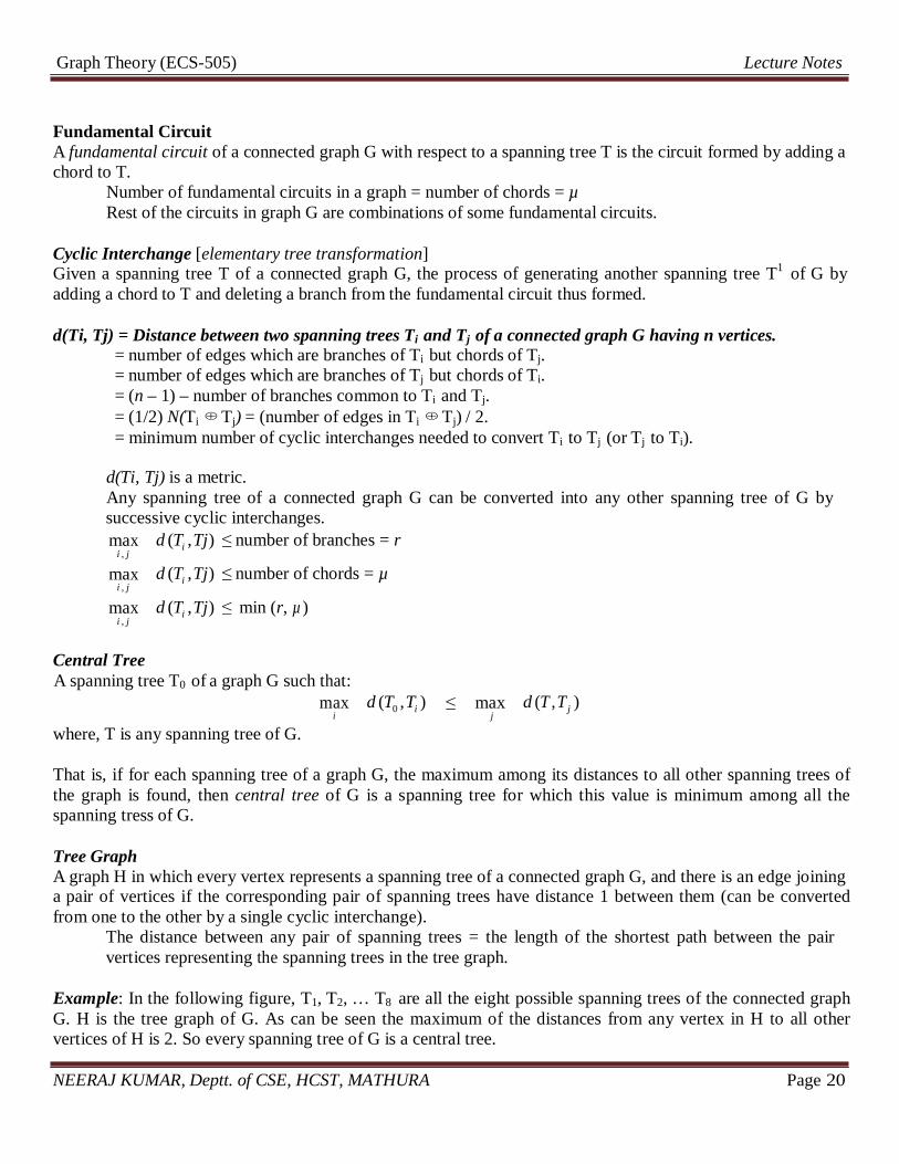
Tree Graph A graph H in which every vertex represents a spanning tree of a connected graph G, and there is an edge joining a pair of vertices if the corresponding pair of spanning trees have distance 1 between them (can be converted from one to the other by a single cyclic interchange). The distance between any pair of spanning trees = the length of the shortest path between the pair

vertices representing the spanning trees in the tree graph.

Example: In the following figure, T1, T2, … T8 are all the eight possible spanning trees of the connected graph G. H is the tree graph of G. As can be seen the maximum of the distances from any vertex in H to all other vertices of H is 2. So every spanning tree of G is a central tree.



T1 T2

T5 T8

T7 T6

Spanning Tree of a weighted graph

T3 T4

H

In a connected weighted graph G,

weight of a spanning tree T of G = sum of the weights of all branches of T . Shortest Spanning Tree (Minimal Spanning Tree) of G = a spanning tree of G having the minimum

weight.

Theorem 12 A spanning tree T of a connected weighted graph G is a Shortest Spanning Tree if and only if there exists no other spanning tree T’ at a distance 1 from T, such that weight of T’ is less than that of T.

Kruskal’s Algorithm to find a shortest spanning tree of a connected weighted graph G having n vertices.

1. Arrange all edges of G in a list L in order of non-decreasing weights. 2. Initialize a subgraph T of G as containing all vertices of G but no edges. 3. While (number of edges in T < n–1)

a. From the list L, select the edge e with the minimum weight. b. If on adding e to T, no circuit would be formed, then add e to T. c. Delete e from L.

4. Return T [which is a minimum spanning tree of G].

Example The adjoining figure shows the operation of Kruskal’s algorithm on a weighted graph. For each iteration of the algorithm, the edges shown as dashed line are the ones still in the list L, the edges shown as solid line are the ones already added to T and deleted from L, the edges not shown are the ones which have been deleted from L but not added to T.

Notice that at any time, T is a forest containing all the vertices and some of the edges of G. The number of components in T is reduced by 1 on the addition of every edge from L to T, until finally it has only one component.


b ∞

5

3 0 15 ∞ ∞


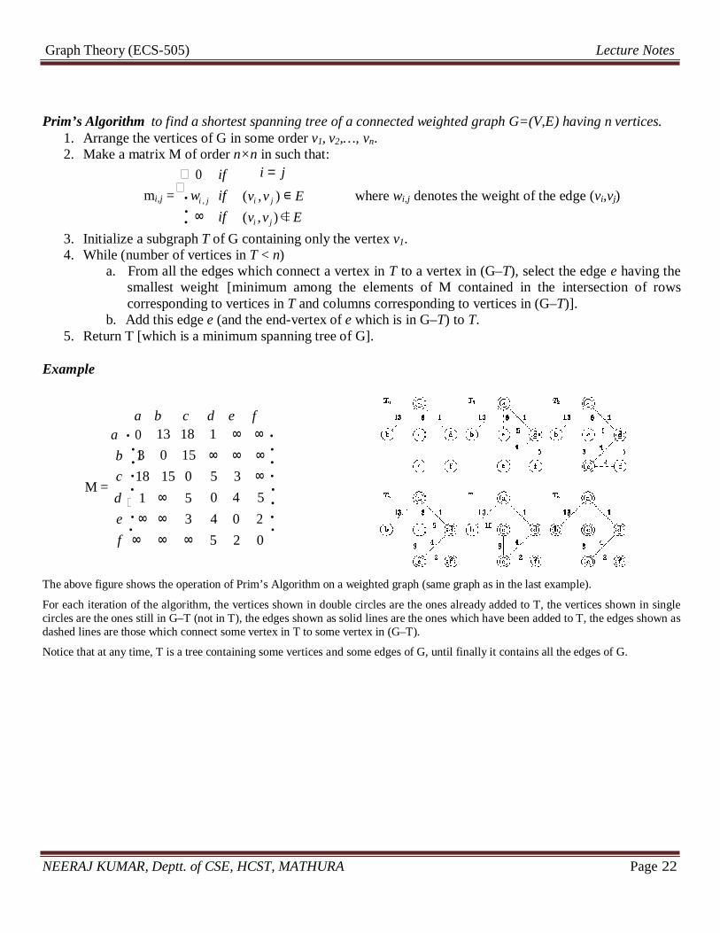
Prim’s Algorithm to find a shortest spanning tree of a connected weighted graph G=(V,E) having n vertices. 1. Arrange the vertices of G in some order v1, v2,…, vn. 2. Make a matrix M of order n×n in such that:

0 if i = j

mi,j = wi , j if ∞ if

(vi , v j ) ∈ E (v , v ) ∉ E

where wi,j denotes the weight of the edge (vi,vj)

i j

3. Initialize a subgraph T of G containing only the vertex v1. 4. While (number of vertices in T < n)

a. From all the edges which connect a vertex in T to a vertex in (G–T), select the edge e having the smallest weight [minimum among the elements of M contained in the intersection of rows corresponding to vertices in T and columns corresponding to vertices in (G–T)].

b. Add this edge e (and the end-vertex of e which is in G–T) to T. 5. Return T [which is a minimum spanning tree of G].

Example

a b c d e f a 0 13 18 1 ∞ ∞

1

c 18 15 0 M =

d 1 ∞ 5 e ∞ ∞ 3

5 3 ∞

0 4 4 0 2

f ∞ ∞ ∞ 5 2 0

The above figure shows the operation of Prim’s Algorithm on a weighted graph (same graph as in the last example).

For each iteration of the algorithm, the vertices shown in double circles are the ones already added to T, the vertices shown in single circles are the ones still in G–T (not in T), the edges shown as solid lines are the ones which have been added to T, the edges shown as dashed lines are those which connect some vertex in T to some vertex in (G–T).

Notice that at any time, T is a tree containing some vertices and some edges of G, until finally it contains all the edges of G.


trees and fundamental circuits - neeraj kumargraph+theory... · graph theory (ecs-505) lecture...

Documents