triangulaciones eficientes del hipercubo
TRANSCRIPT

Dos problemas de combinatoria geometrica:
Triangulaciones eficientes del hipercubo;
Grafos planos y rigidez.
(Two problems in geometric combinatorics:
Efficient triangulations of the hypercube;
Planar graphs and rigidity).
David Orden MartınUniversidad de Cantabria
Tesis doctoral dirigida por el Profesor Francisco Santos Leal.
Santander, Marzo de 2003.

2

Indice
Agradecimientos iii
Preambulo v
Preamble vii
1 Introduccion y Preliminares 11.1 Triangulaciones y subdivisiones de politopos . . . . . . . . . . . . . . 1
1.1.1 Preliminares sobre Teorıa de Politopos . . . . . . . . . . . . . 21.1.2 Triangulaciones de cubos . . . . . . . . . . . . . . . . . . . . 6
1.2 Teorıa de Grafos . . . . . . . . . . . . . . . . . . . . . . . . . . . . . 111.2.1 Preliminares y relaciones con politopos . . . . . . . . . . . . . 111.2.2 Inmersiones planas de grafos: Teorema de Tutte . . . . . . . 15
1.3 Teorıa de Rigidez . . . . . . . . . . . . . . . . . . . . . . . . . . . . . 201.3.1 La matriz de rigidez . . . . . . . . . . . . . . . . . . . . . . . 201.3.2 Tensiones y grafos recıprocos . . . . . . . . . . . . . . . . . . 231.3.3 Rigidez infinitesimal y grafos isostaticos . . . . . . . . . . . . 26
1.4 Pseudo-triangulaciones de cuerpos convexos y puntos . . . . . . . . . 291.4.1 Pseudo-triangulaciones de cuerpos convexos . . . . . . . . . . 291.4.2 Pseudo-triangulaciones de puntos . . . . . . . . . . . . . . . . 31
1.5 Resultados y Problemas abiertos . . . . . . . . . . . . . . . . . . . . 351.5.1 Triangulaciones eficientes de cubos . . . . . . . . . . . . . . . 351.5.2 Grafos sin cruces, rigidez y pseudo-triangulaciones . . . . . . 36
1 Introduction and Preliminaries 411.1 Triangulations and subdivisions of polytopes . . . . . . . . . . . . . 41
1.1.1 Preliminaries about Polytope Theory . . . . . . . . . . . . . . 421.1.2 Triangulations of cubes . . . . . . . . . . . . . . . . . . . . . 46
1.2 Graph Theory . . . . . . . . . . . . . . . . . . . . . . . . . . . . . . . 501.2.1 Preliminaries and relations with polytopes . . . . . . . . . . . 511.2.2 Plane embeddings of graphs: Tutte’s Theorem . . . . . . . . 54
1.3 Rigidity Theory . . . . . . . . . . . . . . . . . . . . . . . . . . . . . . 591.3.1 The rigidity matrix . . . . . . . . . . . . . . . . . . . . . . . . 591.3.2 Stresses and reciprocal graphs . . . . . . . . . . . . . . . . . . 62
i

ii
1.3.3 Infinitesimal rigidity and isostatic graphs . . . . . . . . . . . 651.4 Pseudo-triangulations of convex bodies and points . . . . . . . . . . 67
1.4.1 Pseudo-triangulations of convex bodies . . . . . . . . . . . . . 681.4.2 Pseudo-triangulations of points . . . . . . . . . . . . . . . . . 69
1.5 Results and Open problems . . . . . . . . . . . . . . . . . . . . . . . 731.5.1 Efficient triangulations of cubes . . . . . . . . . . . . . . . . . 731.5.2 Non-crossing graphs, rigidity and pseudo-triangulations . . . 74
2 Asymptotically efficient triangulations of the d-cube 792.1 Introduction . . . . . . . . . . . . . . . . . . . . . . . . . . . . . . . . 792.2 Overview of the method and results . . . . . . . . . . . . . . . . . . 822.3 Polyhedral subdivision of P ×∆k1+···+km−1 induced by one of P ×∆m−1 842.4 Triangulation of P ×∆k1+···+km−1 induced by one of P ×∆m−1 . . . 862.5 A triangulation of P ×Q . . . . . . . . . . . . . . . . . . . . . . . . 882.6 Interpretation of our method via the Cayley Trick . . . . . . . . . . 922.7 Computation of ρl,m . . . . . . . . . . . . . . . . . . . . . . . . . . . 95
2.7.1 Smallest weighted efficiency of triangulations of I2 ×∆m−1 . 952.7.2 Smallest weighted efficiency of triangulations of I3 × ∆m−1,
for m = 2, 3 . . . . . . . . . . . . . . . . . . . . . . . . . . . . 97
3 The polytope of non-crossing graphs on a planar point set 1013.1 Introduction . . . . . . . . . . . . . . . . . . . . . . . . . . . . . . . . 1013.2 The graph of all pseudo-triangulations of A . . . . . . . . . . . . . . 105
3.2.1 Marked non-crossing graphs on A. . . . . . . . . . . . . . . . 1093.3 The polyhedron of marked non-crossing graphs on A . . . . . . . . . 1103.4 Valid choices of f . . . . . . . . . . . . . . . . . . . . . . . . . . . . . 1163.5 Points in special position . . . . . . . . . . . . . . . . . . . . . . . . . 120
3.5.1 The graph of all pseudo-triangulations of A . . . . . . . . . . 1203.5.2 The case with only interior collinearities . . . . . . . . . . . . 1233.5.3 Boundary collinearities . . . . . . . . . . . . . . . . . . . . . . 128
4 Planar minimally rigid graphs and pseudo-triangulations 1314.1 Introduction . . . . . . . . . . . . . . . . . . . . . . . . . . . . . . . . 1314.2 Embedding combinatorial pseudo-triangulations . . . . . . . . . . . . 1324.3 3-connectedness of G . . . . . . . . . . . . . . . . . . . . . . . . . . . 1374.4 Laman graphs admit c.p.p.t. labelings. . . . . . . . . . . . . . . . . . 1404.5 Infinitesimally rigid graphs admit c.p.t. labelings. . . . . . . . . . . . 145
5 Rigidity circuits, reciprocal diagrams and pseudo-triangulations 1495.1 Introduction . . . . . . . . . . . . . . . . . . . . . . . . . . . . . . . . 1495.2 Non-crossing spherical frameworks with non-crossing reciprocals . . . 1525.3 Proof of Theorems 5.2.1 and 5.2.3 . . . . . . . . . . . . . . . . . . . 1545.4 Rigidity circuits. The case of pseudo-triangulations . . . . . . . . . . 156

Agradecimientos
Quiero expresar aquı mi gratitud a todas las personas que de una u otra formame han apoyado durante la realizacion de este trabajo. Muy especialmente a mispadres, pues entre lo mucho que les debo esta el haber puesto siempre la mejorde sus voluntades para allanar el camino de la vida academica que ahora termino.Tanto ellos como mi hermano aportaron palabras de aliento al dıa a dıa de unainvestigacion que muchas veces les era lejana. Ademas de su apoyo, a Encarna leagradezco tambien de una forma especial su companıa durante este tiempo.
Mi reconocimiento es tambien para aquellos amigos y companeros que, cada unoen su medida, colaboraron y pusieron en tantas ocasiones un necesario parentesisen mi trabajo. Asimismo, quiero hacer constar mi gratitud por el apoyo, a menudoincomparable en lo profesional y personal, de Paco Santos, sin cuya guıa este tra-bajo habrıa resultado a buen seguro mucho menos llevadero. Otros miembros deldepartamento, desde la entrada en esta facultad hasta hoy, facilitaron tambien miandadura y me aportaron en ocasiones sus opiniones y consejos, por lo que les estoyagradecido.
Finalmente, quiero mencionar a: Gunter Ziegler, en cuyo grupo de la TechnischeUniversitat Berlin realice una estancia en otono de 2000. Emo Welzl y JurgenRichter-Gebert, que permitieron mi asistencia a sus cursos en el ETH de Zurich.Komei Fukuda y Marc Noy, quienes accedieron a recomendar mi investigacion. Jesusde Loera, por su calurosa acogida durante mi estancia en la University of Californiaat Davis en el otono de 2001, y por ayudarme a intentar mejorar algunos calculos deesta tesis e invitarme a impartir una conferencia en Agosto de 2002. Ferran Hurtado,a cuya iniciativa debo tanto mi inclusion en una accion integrada de la UniversitatPolitecnica de Catalunya como la solicitud de otras ayudas. Franz Aurenhammer,por aceptar mi estancia en la Technische Universitat Graz en el proximo otono.Gunter Rote, que colaboro en parte de los resultados de esta tesis. Ruth Haas,Brigitte Servatius, Hermann Servatius, Diane Souvaine, Ileana Streinu y WalterWhiteley tambien aportaron conversaciones utiles a algunos de estos resultados.
iii

iv

Preambulo
Esta tesis esta dividida en dos partes independientes, aunque ambas proporcionanconstrucciones en combinatoria geometrica. En la primera parte, se aborda el estudiode metodos para construir triangulaciones “sencillas” de hipercubos de dimensionalta. Se ha demostrado que la obtencion de triangulaciones eficientes del d-cuboregular Id = [0, 1]d tiene aplicaciones de interes como el calculo de puntos fijoso la resolucion de ecuaciones diferenciales por metodos de elementos finitos. Enparticular, se ha dedicado especial atencion a tratar de determinar la triangulacionmas pequena (en numero de sımplices 1 ) o, al menos, el comportamiento asintoticode ese numero mınimo de sımplices. Los resultados previos se deben a Sallee (1984)y Haiman (1991). En el Capıtulo 2 desarrollamos una construccion para obtenertriangulaciones eficientes del producto de dos politopos generales. Aplicado al casoparticular del producto de dos cubos, demostramos que este metodo mejora las cotasobtenidas por Haiman para el tamano asintotico de una triangulacion del d-cubo.Nuestra construccion comienza con una triangulacion “eficiente” del producto entreun cubo y un sımplice de dimensiones pequenas. Este trabajo tiene una partepuramente teorica (como usar las triangulaciones de dimension baja en objetos dedimension alta) y una parte computacional (el calculo de la triangulacion optima,para nuestros propositos, de los objetos de dimension baja).
La segunda parte de la tesis trata sobre las relaciones entre grafos planos, rigidezy pseudo-triangulaciones 2 de un conjunto de puntos en el plano. Estas tienen ricaspropiedades combinatorias y han sido aplicadas con un amplia variedad de propositos(planificacion de movimientos, visibilidad, estructuras de datos cineticas) durante laultima decada. En el Capıtulo 3 consideramos un conjunto A de puntos en el planoy, utilizando propiedades que relacionan las pseudo-triangulaciones con la teorıaclasica de la rigidez (algunos de cuyos precursores son Euler y Cauchy), construimosun politopo simple cuyos vertices son todas las posibles pseudo-triangulaciones de A.Al contrario que las construcciones similares propuestas previamente para triangu-laciones, podemos describir completamente las ecuaciones de las facetas de nuestropolitopo, lo que implica que se puede utilizar programacion lineal para optimizarfuncionales sobre el. Por otro lado, la estructura de caras del politopo es esencial-mente la estructura de todos los grafos sin cruces que es posible dibujar en A. La
1Un d-sımplice es la envolvente convexa de d + 1 puntos afınmente independientes.2Un pseudo-triangulo es un polıgono simple con exactamente tres vertices convexos.
v

vi
construccion del politopo sirve incluso para un conjunto de puntos en posicion nogeneral, lo que conduce a una definicion natural de pseudo-triangulacion para esecaso.
En cuanto a sus relaciones con rigidez, Streinu (2000) demostro que las pseudo-triangulaciones puntiagudas 3 son grafos planos minimalmente rıgidos. Demostramosque el inverso es tambien cierto: todo grafo plano minimalmente rıgido admite unainmersion como pseudo-triangulacion puntiaguda en R
2, incluso bajo ciertas res-tricciones combinatorias como la imposicion a priori de los tres angulos convexosde cada cara. Este tipo de problemas de inmersion de grafos han sido ampliamenteestudiados en la literatura, y nuestro resultado proporciona una caracterizacion delos grafos planos minimalmente rıgidos que se anade a la debida a Laman. Yendomas lejos, obtenemos varios resultados que nos conducen a conjeturar que se puedeextender la anterior caracterizacion para relacionar grafos planos rıgidos y pseudo-triangulaciones generales.
Finalmente, el Capıtulo 5 tiene que ver con la relacion de Maxwell (1864) entrediagramas de fuerzas y figuras recıprocas. Obtenemos las condiciones para que undiagrama de fuerzas plano con un unico equilibrio tenga un recıproco sin cruces.En particular, mostramos que si el diagrama es una pseudo-triangulacion con exac-tamente un vertice no puntiagudo, entonces el recıproco es tambien una pseudo-triangulacion del mismo tipo.
3En las que todo vertice es puntiagudo, e.d. tiene un angulo incidente mayor de 180 grados.

Preamble
This thesis is divided into two independent parts, although both of them provideconstructions in geometric combinatorics. The first part deals with the study ofmethods to construct “simple” triangulations of high dimensional hypercubes. Ob-taining efficient triangulations of the regular d-cube Id = [0, 1]d has been proved tohave interesting applications such as calculating fixed points or solving differentialequations by finite element methods. In particular, it has brought special attentionthe problem of finding the smallest size (in number of simplices 4 ) of a triangulationor, at least, the asymptotic behavior of this smallest number of simplices. Previousresults are by Sallee (1984) and Haiman (1991). In Chapter 2 we develop a con-struction to obtain efficient triangulations of the product of two general polytopes.Applied to the particular case of the product of two cubes, we show this method toimprove the bounds obtained by Haiman for the asymptotic size of a triangulationof the d-cube. Our construction starts from an “efficient” triangulation of the prod-uct of a cube and a simplex of small dimensions. This work has a purely theoreticpart (how to use the triangulations of small dimensional objects in high dimensionalones) and a computational part (the computation of the optimal triangulation, forour purposes, of the small dimensional objects).
The second part of the thesis deals with the relations between planar graphs,rigidity and pseudo-triangulations 5 of a planar point set. These have rich combi-natorial properties and have been applied with a wide range of purposes in compu-tational geometry (motion planning, visibility, kinetic data structures) during thelast decade. In Chapter 3 we consider a planar point set A and, using propertieswhich relate pseudo-triangulations to the classical rigidity theory (somme of whoseprecursors are Euler and Cauchy), we construct a simple polytope whose verticesare all the possible pseudo-triangulations of A. Contrary to previously proposedsimilar constructions for triangulations, we can completely describe the equationsfor the facets of our polytope, what implies that linear programming can be used tooptimize functionals on it. In addition, the face poset of the polytope is essentiallythe poset of all non-crossing graphs which can be drawn on A. The construction ofthe polytope works even for a point set in non-general position, leading to a naturaldefinition of pseudo-triangulation for that case.
4A d-simplex is the convex hull of d + 1 affinely independent points.5A pseudo-triangle is a simple polygon with exactly three convex vertices.
vii
viii
Concerning their relations with rigidity, Streinu (2000) proved that pointed 6
pseudo-triangulations are minimally rigid planar graphs. We prove the converse tobe true as well in Chapter 4: Every minimally rigid planar graph admits an em-bedding in R
2 as a pointed pseudo-triangulation, even under certain combinatorialrestrictions such as fixing a priori the three convex angles of each face. This typeof embeddability problems have been thoroughly studied in the literature, and ourresult provides a characterization of minimally rigid planar graphs which adds to thewell-known one due to Laman. Going further, we obtain several results leading usto conjecture that the above characterization can be extended to relate rigid planargraphs and general pseudo-triangulations.
Finally, Chapter 5 is related to Maxwell’s relation (1864) between diagrams offorces and reciprocal figures. We obtain the conditions of a planar diagram of forceswith a unique equilibrium to have a non-crossing reciprocal. In particular, we showthat if the diagram is a pseudo-triangulation with exactly one non-pointed vertex,then the reciprocal is again such a pseudo-triangulation.
6In which every vertex is pointed, i.e. has an incident angle greater than 180 degrees.

Capıtulo 1
Introduccion y Preliminares
En este capıtulo nuestra intencion es proporcionar la base para una comprensionmas sencilla del trabajo presentado en los capıtulos siguientes. A pesar de que estoshan sido escritos con el proposito de ser lo mas auto-contenidos posible, hay algunasnociones y resultados que pueden ser o no familiares para el lector. Comenzamosaquı por los mas basicos, de manera que se puedan introducir lectores de distintoscampos. Ademas, los ejemplos y construcciones han sido elegidos de modo quejugaran un papel mas adelante en la obtencion y discusion de los resultados.
La mayor parte de los enunciados en este capıtulo introductorio aparecen sin de-mostracion. No obstante, siempre damos referencias en las que pueden encontrarsey donde un lector interesado puede buscar informacion adicional. Sı incluimos aque-llas demostraciones que van a resultar cruciales en el resto de los capıtulos, bien porla tecnica utilizada, o bien porque vayamos a hacer uso de ellas mas adelante.
La estructura del capıtulo es como sigue: en la primera seccion introducimosalgo de Teorıa de Politopos, para centrarnos a continuacion en triangulaciones decubos. La segunda seccion esta dedicada a Teorıa de Grafos, comenzando por unsumario de vocabulario y resultados basicos. Mostramos despues dos conexiones conpolitopos, antes de dar una respuesta parcial al problema de inmersion de grafos,que va a resultar un resultado clave en el Capıtulo 4. Posteriormente, trasladamosnuestra atencion a la rigidez de grafos inmersos en el plano y enunciamos una seriede nociones y resultados que terminan con la definicion de rigidez en la que estamosinteresados. La cuarta seccion esta dedicada a presentar las pseudo-triangulaciones,tanto de cuerpos convexos como de puntos. Finalmente, en la ultima seccion es-pecificamos los resultados obtenidos en esta tesis, ası como algunos problemas quequedan abiertos y pueden resultar objeto de un futuro trabajo.
1.1 Triangulaciones y subdivisiones de politopos
Las raıces historicas del estudio de politopos se remontan a los matematicos de laantigua Grecia. De hecho, los polıgonos y poliedros parecen haber estado entrelos mas tempranos objetos de una investigacion matematica sistematizada, cuyo
1

2 Capıtulo 1. Introduccion y Preliminares
primer resultado resenable es la enumeracion de los famosos Solidos Platonicos, queson la solucion al problema de encontrar todos los cuerpos convexos regulares dedimension 3; aquellos cuyas caras son copias de un mismo polıgono convexo y para losque el numero de caras que inciden en cada vertice es siempre el mismo. Este puedeser considerado el punto de partida del estudio de las conexiones entre geometrıa ycombinatoria, lo que desde entonces hasta nuestros dıas, pasando por el Libro XIIde los Elementos de Euclides, ha sido una de las mas resenables caracterısticas delos politopos.
1.1.1 Preliminares sobre Teorıa de Politopos
Entre los objetos basicos en geometrıa se cuentan puntos, rectas, planos o hiper-planos, subespacios afines de dimensiones 0, 1, 2 y d − 1 respectivamente, en unespacio afın R
d. Concentremos nuestra atencion en conjuntos finitos de puntos eti-quetados y que generen R
d. Los conjuntos de puntos que consideraremos a lo largode esta tesis estaran habitualmente en posicion general, lo que quiere decir que todosubconjunto de n + 1 puntos genera R
n. Pero las definiciones y resultados en estasubseccion sirven igualmente para el caso en que aparezcan degeneraciones.
Como de costumbre, los elementos de Rd se pueden ver bien como puntos o bien
como vectores. Es decir, se puede considerar Rd como un espacio afın o vectorial.
La siguiente definicion establece, desde ambos puntos de vista, la que probablementesea la nocion crucial en Teorıa de Politopos:
Definicion 1.1.1 • Un conjunto de puntos K ⊆ Rd es convexo si para cualquier
par de puntos x, y ∈ K, el segmento recto [x, y] = λx + (1− λ)y : 0 ≤ λ ≤ 1esta contenido en K.
• Un conjunto no vacıo de vectores Y ⊆ Rd es un cono si para cada subconjunto
finito de vectores y1, . . . , yk ⊆ Y todas sus combinaciones lineales con coe-ficientes positivos estan contenidas en Y . Por convenio, todo cono contiene elvector cero (obtenido como combinacion del conjunto vacıo).
Esta claro que toda interseccion de conjuntos convexos es a su vez un convexo,por lo que la envolvente convexa de K, definida como la interseccion de todos losconjuntos convexos en R
d que contienen a K, es el menor convexo conteniendo a K:
conv(K) :=⋂K ′ ⊆ R
d : K ′ ⊇ K, K ′ convexo
Para el caso de un conjunto finito de puntos K = x1, . . . , xn ⊆ Rd, la envol-
vente convexa coincide con el conjunto de todas sus combinaciones convexas
conv(K) = λ1x1 + · · ·+ λnxn : λi ≥ 0,n∑
i=1
λi = 1
Analogamente, para un conjunto finito de vectores Y = v1, . . . , vn ⊆ Rd, la
envolvente conica de Y , definida como la interseccion de todos los conos en Rd que
contienen a Y , se puede expresar como:

1.1. Triangulaciones y subdivisiones de politopos 3
cone(Y ) = µ1y1 + · · ·+ µnyn : µi ≥ 0
Antes de estar preparados para introducir dos versiones diferentes del principalobjeto de estudio en esta seccion, los poliedros y politopos convexos, necesitamosdefinir la suma de Minkowski de dos conjuntos P, Q ⊆ R
d como
P + Q := p + q : p ∈ P, q ∈ Q
A lo largo de esta tesis no vamos a considerar poliedros o politopos no convexos.Es por esto por lo que en adelante eliminaremos la palabra “convexo” cuando nosrefiramos a ellos:
Definicion 1.1.2 En un espacio afın Rd:
• Un V-poliedro es la suma de Minkowski de los dos siguientes conjuntos; laenvolvente convexa de un conjunto finito de puntos, y la envolvente conica deun conjunto finito de vectores:
conv(K) + cone(Y )
• Un H-poliedro es una interseccion de un numero finito de semiespacios cerra-dos.
• Un V-politopo es un V-poliedro acotado, esto es, la envolvente convexa de unconjunto finito de puntos conv(K).
• Un H-politopo es un H-poliedro acotado, esto es, una interseccion de unnumero finito de semiespacios cerrados que no contiene ningun rayo x + µy :µ ≥ 0 para cualquier y = 0.
La equivalencia de la V-definicion y la H-definicion parece “geometricamenteclara”. Sin embargo, no es un hecho trivial de probar. Referimos al lector a [84]para una demostracion del siguiente enunciado, del cual se sigue como consecuenciala equivalencia de las V y H-definiciones para politopos. Mencionemos unicamenteque en el fondo de la demostracion esta el Lema de Farkas o, en otras palabras, ladualidad de la programacion lineal.
Teorema 1.1.3 (Teorema fundamental para poliedros) Un subconjunto P ⊆R
d es un V-poliedro si, y solo si, es un H-poliedro.
La dimension dim(P ) de un politopo o poliedro es la de su envolvente afın, lainterseccion de todos los subespacios afines que contienen a P . Un d-politopo es unpolitopo de dimension d en algun R
e (e ≥ d). El primer ejemplo de d-politopo quevamos a considerar es, en el sentido combinatorio, el “mas pequeno”:

4 Capıtulo 1. Introduccion y Preliminares
Ejemplo 1.1.4 Un d-sımplice τ es la envolvente convexa de d+1 puntos afınmenteindependientes cualesquiera en algun R
e. Por ejemplo, los triangulos y los tetrae-dros son los 2-sımplices y 3-sımplices, respectivamente. Es facil ver que todos losd-sımplices son afınmente isomorfos al d-sımplice estandar ∆d definido como
∆d := conve1, . . . , ed+1, donde ei es el i-esimo vector unidad en Rd+1.
x
y
z
Figura 1.1: El 2-sımplice estandar ∆2.
Intuitivamente esta claro lo que son las caras de un politopo; su caracterizacionmatematica se basa en funcionales lineales:
Definicion 1.1.5 Sea P ⊆ Rd un politopo convexo. Una cara de P es un conjunto
de la formaF = P ∩ x ∈ R
d : 〈c, x〉 = c0,donde c ∈ R
d, c0 ∈ R y la desigualdad 〈c, x〉 ≤ c0 se satisface para todos los puntosx ∈ P . La dimension de una cara es la de su envolvente afın.
Observese que tanto el propio P como ∅ son caras del politopo P , definidasrespectivamente por las desigualdades 〈0, x〉 ≤ 0 y 〈0, x〉 ≤ 1. Se les llama caraimpropia y cara trivial. Los vertices, aristas y facetas de P son respectivamentelas caras de dimensiones 0, 1 y dim(P ) − 1; en particular, los vertices de P , deno-tados vert(P ), son las caras no vacıas minimales, y las facetas son las caras propiasmaximales. El k-esqueleto de un politopo es la union de sus caras k-dimensionales.La estrella de una cara F , denotada star(F ), se define como el conjunto de carascontenidas en la union de todas las facetas que contienen a F .
Los dos siguientes tipos especiales de politopos nos introducen en el estudio dela combinatoria de estas estructuras geometricas:
Definicion 1.1.6 Dado un politopo P de dimension d,
• Se dice que P es simple si todo vertice esta exactamente en d facetas.

1.1. Triangulaciones y subdivisiones de politopos 5
• A P se le llama simplicial si todas sus facetas son sımplices.
La informacion combinatoria de un politopo P va a estar codificada por su es-tructura de caras. Para estudiar esta, necesitamos en primer lugar algunas nocionessobre conjuntos parcialmente ordenados, o “posets” (abreviatura de partially orderedsets). El lector interesado en el tema puede encontrar un estudio detallado en [16,Capıtulo 11].
Definicion 1.1.7 Un poset (S,≤) es un conjunto finito S junto con una relacion“≤” reflexiva, antisimetrica y transitiva.
• Un poset es acotado si tiene un unico elemento minimal y un unico elementomaximal.
• Un poset Booleano es uno isomorfo al poset Bk = (2[k],⊆) de todos los sub-conjuntos de un conjunto de k elementos.
• Una cadena en un poset es un conjunto totalmente ordenado; la longitud deuna cadena es su numero de elementos menos 1.
• Un poset S es graduado si es acotado y todas las cadenas maximales tienen lamisma longitud, que es llamada longitud o rango de S.
• Un retıculo es un poset acotado tal que todo par de elementos x, y ∈ S tienenuna unica cota superior minimal y una unica cota inferior maximal en S.
• El ideal inferior de un elemento x en (S,≤) es el conjunto y ∈ S : y ≤ x. Elfiltro superior es y ∈ S : y ≥ x.
El siguiente resultado, bien conocido, describe la estructura de poset de las carasde un politopo, que es habitualmente referida como poset de caras:
Teorema 1.1.8 Para todo politopo P , el poset de todas sus caras parcialmente or-denadas por la inclusion es un retıculo graduado de longitud dim(P ) + 1. Por eso,se le llama tambien retıculo de caras de P y se denota L(P ).
Ejemplo 1.1.9 En la Figura 1.2 mostramos el poset de caras de un pentagono con-vexo (izquierda), que es un retıculo de longitud 3, y el de un 3-sımplice (derecha),que es un retıculo Booleano de longitud 4.
Como avanzamos arriba, el retıculo de caras es la nocion apropiada para definirequivalencia combinatoria de politopos: dos politopos P y Q se dicen combinatoria-mente equivalentes si sus retıculos de caras son isomorfos, L(P ) ∼= L(Q).

6 Capıtulo 1. Introduccion y Preliminares
4
1 2
3
1 2
3
4
1 2
4
1
3
4
2
3
1 2
3
4
1 2
3
4
2
4
3
1 2
3
4
1
Figura 1.2: Retıculos de caras de un pentagono convexo y un 3-sımplice.
1.1.2 Triangulaciones de cubos
Cuando se tiene un objeto geometrico complicado (por ejemplo, un politopo “grande”),a veces resulta conveniente descomponerlo en partes mas pequenas y sencillas parasimplificar su estudio:
Definicion 1.1.10 Un complejo politopal C se define como una coleccion finita depolitopos en R
d tal que:
(i) El politopo vacıo esta en C,
(ii) Si P ∈ C, entonces todas las caras de P estan tambien en C, y
(iii) La interseccion P ∩Q de dos politopos P, Q ∈ C es una cara de ambos.
La dimension dim(C) es la mayor dimension de un politopo en C. El conjunto soportede C es el conjunto de puntos |C| := ∪P∈CP .
Como antes, la estructura combinatoria de un complejo politopal C es capturadapor su poset de caras (C,⊆), dado por el conjunto de politopos en C ordenados porinclusion. A continuacion aparecen las definiciones que dan nombre a esta seccion:
Definicion 1.1.11 Dado un d-politopo P :
• Una subdivision politopal, o simplemente subdivision, de P es un complejopolitopal C tal que su conjunto soporte es |C| = P .
• Una triangulacion de P es una subdivision en la que todos los politopos en Cson sımplices.

1.1. Triangulaciones y subdivisiones de politopos 7
• Dada una subdivision C de P , un refinamiento es otra subdivision C′ tal quetodo politopo de C es una union de politopos de C′.
Una descomposicion de P en d-sımplices que no se solapan y que no cumplen lacondicion (iii) de la Definicion 1.1.10 se llama diseccion o, en caso de que todos lospolitopos sean sımplices, diseccion simplicial. En particular, a lo largo de esta tesisestamos interesados en subdivisiones, triangulaciones y disecciones cuyo conjunto devertices coincide con el de P , esto es, que no anaden vertices nuevos y tales que todovertice es utilizado.
Observacion 1.1.12 La misma definicion sirve para subdivisiones, triangulaciones,refinamientos y disecciones de un conjunto finito de puntos A, considerando elpolitopo definido por su envolvente convexa, excepto porque estamos asumiendoimplıcitamente que solo se pueden utilizar como vertices puntos de A. Ademas, engeneral supondremos que se utilizan todos.
Ejemplo 1.1.13 La Figura 1.3 representa una triangulacion (izquierda) y una di-seccion simplicial (derecha) del cubo 3-dimensional. En el primer caso, la triangu-lacion se compone de 5 sımplices: los cuatro tetraedros obtenidos cortando esquinasno adyacentes y el tetraedro resultante, que usa diagonales opuestas de las carassuperior e inferior. En el segundo caso, el cubo esta partido en dos prismas trian-gulares, para una mejor visualizacion: cada prisma esta triangulado en 3 tetraedros,pero las triangulaciones inducidas en la cara comun a ambos prismas usan diago-nales opuestas. Por lo tanto esos 6 tetraedros no forman una triangulacion, puestoque se viola la condicion (iii) de complejos politopales.
Figura 1.3: Izquierda: Una triangulacion del 3-cubo. Derecha: Una diseccion del3-cubo.
Senalemos aquı que toda subdivision de un politopo P se puede refinar a unatriangulacion. Para ello, se necesitan triangulaciones Ti de cada uno de los politoposPi en la subdivision tales que, para todo par de ındices i, j, Ti y Tj induzcan la mismatriangulacion en Ti ∩ Tj cuando esta se considera como cara de Ti y de Tj . Existenconstrucciones bien conocidas (vease por ejemplo [76]) con esta caracterıstica.

8 Capıtulo 1. Introduccion y Preliminares
El estudio de triangulaciones y sus propiedades ha atraıdo un gran interes durantelas ultimas decadas, especialmente estimulado por los avances en la computacion, quehan conducido a un buen numero de aplicaciones en Geometrıa Computacional, entrelas cuales podemos mencionar las relativas a graficos por ordenador o simulacionespara ingenierıa.
En particular, las triangulaciones de cubos han sido objeto de estudio por masde treinta anos, y se tratan en el segundo capıtulo de esta tesis, donde construimostriangulaciones “pequenas” de cubos.
Definamos el producto de dos politopos generales como P × Q := (p, q) : p ∈P, q ∈ Q. Antes de considerar triangulaciones de cubos, vamos a concentrarnos enuna manera de triangular el producto de dos sımplices ∆k×∆l. La triangulacion quemostramos aquı para un producto de este tipo es interesante por sı misma, debido asu simplicidad y facil representacion. Ademas, este interes quedara completamentejustificado en el Capıtulo 2, donde la generalizamos al producto de un politopo yun sımplice. Un resultado clasico es que todas las triangulaciones de un producto∆k ×∆l tienen el mismo numero de sımplices:
Lema 1.1.14 ([13]) Toda triangulacion de ∆k×∆l tiene exactamente(k+l
k
)sımplices.
Nuestro proposito aquı es dar al lector una triangulacion destacada de ∆k ×∆l,que es conocida y utilizada desde hace tiempo en topologıa algebraica [30], y cuyafacil visualizacion la hace un buen ejemplo de lo util que puede ser la combinatoriapara entender estructuras geometricas en dimensiones altas. Esta utilidad se en-cuentra en el trasfondo de toda la tesis, y puede ser incluso mas explıcita en losCapıtulos 2 y 3.
Asumamos que ∆k y ∆l tienen vertices v0, . . . , vk y w0, . . . , wl respectiva-mente. Entonces el producto ∆k ×∆l tiene por conjunto de vertices
(vi, wj) : 0 ≤ i ≤ k, 0 ≤ j ≤ l,
que se puede representar como las casillas de una cuadrıcula de tamano (k+1)×(l+1)cuyas filas corresponden a vertices de ∆k y cuyas columnas representan vertices de∆l. Vease el Ejemplo 1.1.15.
Consideremos ahora caminos del vertice (v0, w0) al vertice (vk, wl) cuyos pasosaumentan en una unidad bien el subındice de v o bien el de w. En la representacion,si etiquetamos filas y columnas de la cuadrıcula de tal manera que (v0, w0) y (vk, wl)sean respectivamente las casillas inferior izquierda y superior derecha, estos caminoscorresponden a escaleras monotonas, en las que cada paso es un movimiento desdeuna casilla bien a la siguiente por la derecha o bien a la inmediatamente superior.Cada uno de estos caminos selecciona un subconjunto de k+l+1 vertices de ∆k×∆l
y no es difıcil ver que determina un sımplice (k + l)-dimensional.La coleccion de sımplices dada por todos estos caminos, representada por la
coleccion de todas las escaleras monotonas en la cuadrıcula, forma una triangulacionde ∆k × ∆l, que se conoce como triangulacion escalera. Notese que el numero deposibles caminos o escaleras es precisamente
(k+lk
).

1.1. Triangulaciones y subdivisiones de politopos 9
Ejemplo 1.1.15 La siguiente figura muestra la triangulacion escalera del prismatriangular ∆1 ×∆2. En la fila superior aparece la representacion de su conjunto devertices (vi, wj) : 0 ≤ i ≤ 1, 0 ≤ j ≤ 2 como las casillas de una cuadrıcula detamano 2× 3. Debajo mostramos las tres posibles escaleras en esta cuadrıcula y loscorrespondientes tetraedros, que triangulan ∆1 ×∆2.
0v
1v
0v
0v
1v
1v
1v
w0
w1
w2
w1
w2
w0 w
1
w2
w00
v )( , )( ,
)( ,
)( ,
)( ,
)( ,
1∆
2∆
Figura 1.4: La triangulacion escalera de ∆1 ×∆2.
Trasladamos ahora nuestra atencion a la familia de d-cubos regulares Id :=[0, 1]d, d ≥ 0. Las triangulaciones “sencillas” del d-cubo regular tienen varias apli-caciones, como la resolucion de ecuaciones diferenciales por metodos de elementosfinitos o el calculo de puntos fijos (vease, por ejemplo, [72]). En particular, haatraıdo una especial atencion, tanto desde un punto de vista teorico como desde elpractico, la determinacion del menor tamano de una triangulacion de Id (ver [51,Seccion 14.5.2] para un estudio reciente). Puntualicemos que el problema generalde calcular la triangulacion mas pequena de un politopo arbitrario es NP-completoincluso restringiendose a dimension 3, vease [10].
Definicion 1.1.16 El tamano de una triangulacion (o diseccion simplicial) T deld-cubo es su numero de sımplices |T |. El menor tamano de triangulaciones de Id sedenota habitualmente por φd.
Definicion 1.1.17 Dado un d-sımplice τ = conv(p1, . . . , pd+1), su volumen se definecomo
vol(τ) := abs
(∣∣∣∣∣ p1 . . . pd+1
1 . . . 1
∣∣∣∣∣)
/d!
El mınimo volumen de un d-sımplice que utilice los vertices de Id es por tanto1/d!, y puesto que el del d-cubo es 1, el tamano maximo de una triangulacion de Id

10 Capıtulo 1. Introduccion y Preliminares
resulta ser d! En el estudio antes mencionado se pueden encontrar un buen numerode triangulaciones de tamano maximo y de facil construccion.
Si se nos dan dos triangulaciones de un d-cubo para d fija, es facil decidir cual delas dos es “mejor” (o “mas sencilla”); la de menor tamano. Sin embargo, en caso deque tengamos triangulaciones de d-cubos para distintas dimensiones d, necesitamosuna nocion que permita discernir cual de ellas es la mas conveniente. Esta fueenunciada por primera vez por Todd en [72]:
Definicion 1.1.18 La eficiencia de una triangulacion T de un d-cubo se definecomo el numero (|T |/d!)1/d. La menor eficiencia (φd/d!)1/d de triangulaciones de Id
se denota ρd.
Observacion 1.1.19 Por la anterior observacion sobre el tamano maximo de unatriangulacion del d-cubo, la eficiencia de una triangulacion de Id es como mucho 1y, cuanto menor sea, mas eficiente es la triangulacion. En particular, ρd ≤ 1,∀d.
En el segundo capıtulo de esta tesis, presentamos una nueva construccion paratriangular Id, que conduce a buenas eficiencias asintoticas. Dicha construccion estabasada en el siguiente metodo, debido a Haiman [40]:
Sean Tk y Tl triangulaciones de cubos regulares Ik e I l respectivamente. El pro-ducto Tk×Tl de las dos triangulaciones (entendido como el producto por pares de sussımplices) da una descomposicion del cubo Ik × I l = Ik+l en |Tk| · |Tl| subpolitopos,cada uno de ellos isomorfo al producto de sımplices ∆k ×∆l.
Por el Lema 1.1.14, toda triangulacion de ∆k×∆l tiene tamano(k+l
k
). Por tanto,
refinando la subdivision Tk × Tl de manera arbitraria se obtiene una triangulacionde Ik+l de tamano |Tk| · |Tl| ·
(k+lk
), lo que lleva a:
Teorema 1.1.20 (Haiman) Para todos k y l, ρk+lk+l ≤ ρk
kρll.
Esto implica que comenzando con una triangulacion con una cierta eficiencia ρde un cubo Ik, se puede construir una sucesion de triangulaciones de Ink para n ∈ N
con esa misma eficiencia. Lo que sugiere inmediatamente el siguiente resultado:
Corolario 1.1.21 La sucesion (ρn)n∈N
es convergente, y
limn→∞
ρn ≤ ρd ∀d ∈ N.
Demostracion: Fijemos d ∈ N y k ∈ 1, . . . , d. El Teorema de Haiman implicaque, para cada i ∈ N,
ρk+id ≤ ρkk/(k+id)ρd
id/(k+id).
Puesto que la expresion de la derecha converge a ρd cuando i crece, las d subsuce-siones de (ρn)
n∈Nconsistentes en ındices iguales modulo d, y por tanto la propia
sucesion, tienen lımite superior acotado por ρd. Esto se cumple para cada d ∈ N.Un lımite superior acotado por todos los terminos de la sucesion debe coincidir con

1.2. Teorıa de Grafos 11
el lımite inferior.
Denotamos por ρ∞ y llamamos eficiencia asintotica de triangulaciones del cuboal lımite de (ρn)
n∈N. El corolario dice que la eficiencia asintotica de triangulaciones
del cubo regular es a lo sumo la eficiencia mınima ρd para cada d. En particular, lamejor cota superior para ρ∞ antes de nuestro trabajo era ρ∞ ≤ ρ7 = 0.840. En elCapıtulo 2 probamos ρ∞ ≤ 0.8159 con un metodo completamente nuevo.
1.2 Teorıa de Grafos
Los investigadores en la materia coinciden en considerar que el artıculo [31] de Euler(en el que se discutıa el famoso problema de los puentes de Konigsberg) marca elnacimiento de la Teorıa de Grafos. Desde entonces, un buen numero de matematicoshan aportado sus contribuciones a este campo, pero ha sido durante el ultimo siglocuando este ha sido objeto de un gran interes, incrementado durante las ultimasdecadas por la sencillez de la representacion de un grafo en ordenadores y el grannumero de problemas que se pueden modelizar utilizando grafos.
En esta seccion presentamos en primer lugar algunas relaciones entre grafos ypolitopos; la primera de ellas es el politopo de subdivisiones de un polıgono convexoy esta relacionada con los resultados del Capıtulo 3. Las otras son interesantespropiedades de los grafos definidos por vertices y aristas de politopos. Finalmente,enunciamos un resultado de Tutte sobre inmersion de un grafo abstracto como unogeometrico, con puntos de R
2 como vertices y segmentos rectos como aristas.
1.2.1 Preliminares y relaciones con politopos
Las nociones basicas que presentamos aquı le seran familiares al lector. Como re-ferencia general sobre grafos recomendamos [15] o [75], y para cada enunciado deesta seccion especificamos donde se puede encontrar una demostracion.
Definicion 1.2.1 Un grafo es un par de conjuntos G = (V, E) donde V = 1, . . . , nes un conjunto finito de vertices y E ⊆ i, j : i, j ∈ V, i = j es un conjunto dearistas entre los vertices. Normalmente denotaremos las aristas por ij en lugar dei, j.
Por definicion, los grafos que consideramos son simples; no tienen ni lazos (aristasque unen un elemento consigo mismo) ni aristas multiples. En la siguiente definicionresumimos parte del vocabulario basico. Denotamos por
(V2
)el conjunto de todos
los pares, no ordenados, de vertices en V .
Definicion 1.2.2 Sea G = (V, E) un grafo.
• El numero de aristas en E que contienen un vertice v ∈ V se denomina gradode ese vertice.

12 Capıtulo 1. Introduccion y Preliminares
• G es regular de grado k si todo vertice tiene grado k.
• G es completo si E =(V
2
). El grafo completo en n vertices se denota por Kn.
• El grafo obtenido a partir de G mediante el borrado de un conjunto de verticesW ⊆ V se define como la restriccion de G al conjunto de vertices V \W , estoes; G \W := (V \W, E ∩
(V \W2
)).
• El conjunto de vecinos de un vertice v se define como N(v) := w ∈ V :v, w ∈ E.
• Un grafo G0 = (V0, E0) es un subgrafo de G, denotado G0 ⊆ G, si V0 ⊆ V yE0 ⊆ E.
Consideramos tres tipos distinguidos de subgrafos:
• Un camino en G entre dos vertices v1, vk ∈ V (notese que 1, k son subındicesy no necesariamente vi = i) es un subgrafo Gvk
v1⊆ G con conjunto de vertices
V vkv1
= v1, . . . , vk y conjunto de aristas Evkv1
= v1, v2, v2, v3, . . . , vk−1, vk.
• Un k-ciclo en G es un subgrafo Gv1v1⊆ G con V v1
v1= v1, . . . , vk y Ev1
v1=
v1, v2, v2, v3, . . . , vk−1, vk, vk, v1.
• Un Y -grafo en G de extremos v1, v2, v3 ∈ V es un subgrafo compuesto por unvertice w ∈ V \ v1, v2, v3 y caminos Gw
v1, Gw
v2, Gw
v3que son disjuntos excepto
por el punto comun w.
Ası como un tipo especial de grafos que apareceran mas adelante:
• G es un grafo bipartito si V es la union disjunta de dos conjuntos V1, V2 y cadaarista une un vertice de V1 con otro de V2. Se dice completo si sus aristas sontodas las posibles entre V1 y V2. El grafo bipartito completo se denota porKm,n, para m y n los cardinales de los conjuntos.
Los caminos y los ciclos se denotan a menudo por la secuencia de aparicion de susvertices, esto es, (v1, v2, . . . , vk) o (v1, v2, . . . , vk, v1). Otra nocion que nos interesaes la de conexion:
• G es conexo si para cada par de vertices distintos v, w ∈ V hay un camino Gwv
que los une.
• G es k-conexo para k > 1 si para todo v ∈ V el grafo G \ v es (k − 1)-conexo.
Ası, un grafo abstracto G = (V, E) esta dado como un conjunto de verticesjunto con un conjunto de pares no ordenados de vertices, y no se involucra ningunageometrıa. Por otro lado, una inmersion topologica G → S
2 es una aplicacion queenvıa los vertices V a puntos en la 2-esfera y las aristas ij ∈ E a arcos. Se le llamainmersion plana o sin cruces si ningun par de arcos pipj y pkpl correspondientes aaristas no adyacentes ij, kl ∈ E, i, j ∈ k, l tiene un punto en comun.

1.2. Teorıa de Grafos 13
Una inmersion geometrica, o un grafo geometrico G(S) = (V, E, S) se definecomo un grafo G = (V, E) junto con una aplicacion i → pi ∈ S de los vertices Va un conjunto finito de puntos S := p1, . . . , pn ⊂ R
2 en el plano euclıdeo y delas aristas ij ∈ E a segmentos rectos pipj . Analogamente, es plana, o sin cruces, siningun par de segmentos correspondientes a aristas no adyacentes se interseca. ElTeorema de Fary [33] establece que se puede “enderezar” toda inmersion topologicaplana y obtener una inmersion geometrica plana. Por otro lado, toda inmersiongeometrica plana induce de manera trivial una inmersion topologica plana (simple-mente proyectando a S
2). Se dice que un grafo es plano si tiene una inmersion,topologica o geometrica, plana.
Las celdas, o caras, de una inmersion geometrica o topologica se definen comolas componentes conexas del complementario (en R
2 o S2) de la union de aristas y
vertices. Una inmersion geometrica plana tiene exactamente una cara no acotada,comunmente llamada cara exterior.
En esta tesis solo vamos a considerar inmersiones de grafos en R2 o S
2. Usaremoslas notaciones G(S) y G → S
2 para inmersiones geometricas y topologicas, respec-tivamente. En ocasiones quiza abusemos de la notacion y utilicemos el conjuntoimagen S para referirnos a la inmersion geometrica G(S). El siguiente resultadorecoge algunos enunciados interesantes; sus demostraciones se pueden encontrar,por ejemplo, en [77]:
Teorema 1.2.3 Sea G un grafo.
(i) (Teorema de Menger) G es k-conexo si, y solo si, entre cada par de verticeshay k caminos G1, . . . , Gk en G que son disjuntos excepto por los extremos.
(ii) (Teorema de Kuratowski) G es plano si, y solo si, no tiene ningun subgrafohomeomorfo al grafo completo K5 ni al grafo bipartito completo K3,3.
(iii) (Teorema de Whitney) Si G es plano y 3-conexo, entonces todas sus in-mersiones topologicas son equivalentes (tienen las mismas celdas).
(iv) (Teorema de Euler) Si G es conexo y plano, para cada inmersion planaG(S) (o G → S
2) los numeros c de celdas, v de vertices y e de aristas estanrelacionados por
v − e + c = 2
Consideremos ahora la clase de grafos geometricos sin cruces en un conjuntodado de vertices A en el plano R
2. Este tipo de grafos es de interes en GeometrıaComputacional, Combinatoria Geometrica y areas relacionadas. En particular, se hadedicado mucho esfuerzo a la enumeracion, recuento y optimizacion en el conjuntode los maximales de entre estos grafos, es decir, las triangulaciones. Notese queaquı estas se consideran con conjunto de vertices igual a A, como se avanzo en laObservacion 1.1.12. Puesto que cualquier triangulacion de un conjunto de puntoscon cardinal n tiene ni + 2n− 3 aristas, para ni el numero de puntos en el interiorde conv(A), es trivial una cota inferior de 2ni+2n−3 = Ω(4n) grafos sin cruces en A.

14 Capıtulo 1. Introduccion y Preliminares
Una cota superior de tipo O(cn) para una constante c se demostro por primera vezen [5]. El mejor valor hasta la fecha para c es 59 · 8 = 472 [62].
Esta claro que el conjunto de grafos geometricos sin cruces en un conjunto depuntos en el plano forma un poset con respecto a la inclusion de aristas. Sin embargo,hasta el desarrollo de esta tesis su estructura de poset solamente se comprendıabien cuando los puntos estaban en posicion convexa. El artıculo [34] contiene variosresultados enumerativos sobre grafos geometricos con n vertices en posicion convexa.En particular, demuestra que hay Θ((6 + 4
√2)nn−3/2) grafos sin cruces en total y
da formulas explıcitas para cada cardinal fijado.Para puntos en posicion convexa, los grafos sin cruces que contienen todas las
aristas de la envolvente convexa coinciden con las subdivisiones poligonales deln-gono convexo. Es bien conocido que el poset que forman es el opuesto del poset decaras (menos la cara vacıa) del (n− 3)-asociaedro, un politopo simple de dimensionn− 3 con las siguientes propiedades:
• Sus vertices se corresponden con todas las 1n−1
(2n−4n−1
)posibles maneras de poner
parentesis en una cadena de longitud n−1 o, equivalentemente, de multiplicaruna expresion a1a2 . . . an−1 cuando la multiplicacion no es asociativa.
• Dos vertices son adyacentes si corresponden a una sola aplicacion de la leyasociativa.
Ası, los vertices del asociaedro se corresponden con las subdivisiones poligonalesque tienen el maximo numero de aristas, es decir, con triangulaciones.
(12)(34)
((12)3)4) (1(2(34))
(1(23))4 1((23)4)
Figura 1.5: Izquierda: El 2-asociaedro. Derecha: Poset de subdivisiones poligonalesdel 5-gono convexo.
Ejemplo 1.2.4 La Figura 1.5 representa el 2-asociaedro (izquierda), cuyos verticescorresponden a las 5 maneras de poner parentesis en la cadena 1234. Por tanto es unpentagono, cuyo retıculo de caras hemos encontrado ya en la Figura 1.2. Ignorandola cara vacıa, se comprueba que este coincide con el opuesto del poset de subdivisionespoligonales del 5-gono convexo, que mostramos en el dibujo de la derecha.

1.2. Teorıa de Grafos 15
El resultado principal en el tercer capıtulo de esta tesis es una generalizaciondel asociaedro; damos una descripcion del poset de grafos sin cruces para cualquierconjunto de puntos, incluso en posicion no general, como un subconjunto del posetde caras de cierto politopo que construimos.
Para una relacion mas directa entre grafos y politopos, observese que los verticesy aristas de un politopo P (el 1-esqueleto) forman un grafo abstracto, al que sellama el grafo de P . Es natural la pregunta inversa sobre cuando un grafo abstractoes el grafo de un politopo; para 3-politopos la respuesta la da el siguiente resultadoclasico, cuya demostracion original aparece en [66] y una muy comprensible se puedeencontrar en [84]:
Teorema 1.2.5 (Steinitz) G es el grafo de un politopo 3-dimensional si, y solo si,es simple, plano y 3-conexo.
La parte del “si” es la mas complicada de demostrar. Para la parte del “y solosi”, puesto que los grafos de politopos son trivialmente simples y su planaridadpuede comprobarse utilizando proyeccion radial sobre una esfera desde un puntointerior, o una proyeccion lineal sobre un plano desde un punto mas alla de unafaceta, unicamente resta aplicar otro resultado bien conocido:
Teorema 1.2.6 (Balinski [8]) El grafo de un d-politopo es d-conexo.
1.2.2 Inmersiones planas de grafos: Teorema de Tutte
Por ultimo, pero no por ello menos importante, introducimos el problema de in-mersion de grafos. La construccion que presentamos para terminar esta seccion dauna respuesta a la siguiente pregunta: dado un grafo plano y 3-conexo G, ¿comopodemos encontrar una inmersion geometrica en la que, ademas, las celdas seanpolıgonos convexos?
El Dibujo de Grafos (Graph Drawing) es un campo con una historia distinguida, ylas inmersiones planas han recibido una atencion sustancial en la literatura ([33], [73],[74], [28], [25], [63], [9]). Tambien se han considerado recientemente (ver por ejemplo[55]) extensiones de inmersiones de grafos con segmentos rectos a pseudo-rectas. Esnatural preguntarse cuando este tipo de inmersiones se pueden “enderezar”, estoes, cuando se pueden dibujar con segmentos rectos manteniendo a su vez algunasubestructura combinatoria. De hecho, el resultado primordial sobre inmersion degrafos planos, el anteriormente mencionado Teorema de Fary [33], es simplementeun ejemplo de dar respuesta a una cuestion de este tipo.
Una explicacion del transfondo de la siguiente construccion se puede dar facilmentemediante este hecho fısico: asumamos que las aristas de G son gomas elasticas.Tomemos los vertices correspondientes a una celda particular F0 cuyo borde tengam vertices. A continuacion, pinchemos estos vertices en el plano R
2 de modo que F0
se convierta en un m-gono convexo y que todas las gomas elasticas interiores esten

16 Capıtulo 1. Introduccion y Preliminares
en tension. Voila; la figura que se obtiene es una inmersion plana de G en la quetodas las demas celdas vienen dadas como polıgonos convexos que no se solapan.
Para modelizar las gomas elasticas se introduce la nocion de peso wij ∈ R deuna arista ij. Notese que, puesto que estamos considerando aristas no dirigidas, sedebe requerir la condicion de simetrıa wij = wji.
Definicion 1.2.7 Sean G = (V, E) un grafo y w : E → R una asignacion de pesosa sus aristas. Consideremos tambien una asignacion de posiciones i → pi ∈ R
2 a losvertices de G. Se dice que un vertice i ∈ V esta en equilibrio si∑
ij∈E
wij(pi − pj) = 0.
Para un ejemplo, vease la Figura 1.6.
El siguiente importante resultado da una respuesta parcial a esta pregunta:¿Cuando un grafo se puede dibujar en el plano con aristas rectas, de tal maneraque las celdas sean convexas y no se solapen? (Esto ultimo equivale a “sin cruces”)
Teorema 1.2.8 (Tutte) Sea G = (1, . . . n, E) un grafo plano y 3-conexo quetiene una celda (k+1, . . . , n) para algun k < n. Sean pk+1, . . . , pn (en este orden) losvertices de un (n− k)-gono convexo. Finalmente, sea w : E′ → R
+ una asignacionde pesos positivos a las aristas interiores. Entonces:
(i) Existen unas unicas posiciones p1, . . . , pk ∈ R2 para los vertices interiores de
modo que todos ellos estan en equilibrio.
(ii) Todas las celdas de G son polıgonos convexos que no se solapan.
Pese a que dar una demostracion completa de este resultado esta fuera de lospropositos de este capıtulo introductorio, en el resto de esta seccion damos un re-sumen de los pasos de la demostracion que aparece en [60], la cual modificamosligeramente en el Capıtulo 4 para demostrar una version dirigida del Teorema deTutte. Incluımos aquı las nociones, resultados intermedios y demostraciones a lasque nos referiremos en ese capıtulo.Demostracion de (i): Asumamos dadas las posiciones de los puntos pk+1, . . . , pn dela frontera. Sin perdida de generalidad, podemos suponer pn = (0, 0). Consideresela funcion
E(x1, . . . , xk, y1, . . . , yk) =12
∑ij∈E′
wij((xi−xj)2 +(yi−yj)2) =12
∑ij∈E′
wij‖pi−pj‖2,
que es cuadratica y no negativa en todo su dominio. Asumamos que el punto z =(x1, . . . , xk, y1, . . . , yk) tiene al menos una entrada, digamos xl, con un valor absolutogrande. Esto implica que pl esta lejos del punto pn = (0, 0) de la frontera. Puestoque el grafo G es conexo, existe un camino que une pl con pn; para al menos unaarista ij en este camino, la distancia ‖pi − pj‖ tiene que ser grande.

1.2. Teorıa de Grafos 17
Ası, para un α > 0 suficientemente grande, la condicion |z| > α implica E(z) >E(0). Como E es cuadratica, esto implica que es estrictamente convexa (no de-generada con Hessiano definido positivo) y por tanto alcanza su unico mınimo enz : |Z| < α. La afirmacion se sigue puesto que la condicion ∇E = 0 para un puntocrıtico de E:
∂E
∂xl=
∑ij∈E′
wij(xi − xj) = 0 y∂E
∂yl=
∑ij∈E′
wij(yi − yj) = 0, ∀l ∈ 1, . . . , k
es exactamente la condicion de equilibrio para los vertices interiores.
Esquema de la demostracion de (ii): De nuevo, asumamos que las posiciones delos puntos pk+1, . . . , pn del borde estan dadas; por (i) las posiciones de los verticesinteriores estan a su vez unıvocamente determinadas. Una configuracion de puntosası se denomina representacion en equilibrio de G.
Ejemplo 1.2.9 En la Figura 1.6 se muestra una representacion en equilibrio de ungrafo G, junto con los pesos de cada arista interior. Damos una cuadrıcula con elproposito de que el lector pueda comprobar facilmente que los tres vertices interioresestan en equilibrio.
1 11
1 1
1
Figura 1.6: Un grafo en equilibrio.
El interior relativo de (la envolvente convexa de) una coleccion de puntos S :=p1, . . . , pn ⊂ R
2 se define como
relint(S) := n∑
i=1
λipi :n∑
i=1
λi = 1 and λi > 0, ∀i = 1, . . . , n.
El siguiente lema, cuya demostracion es inmediata utilizando la condicion deequilibrio, da una propiedad que resulta ser fundamental en el Teorema de Tutte.El enunciado puede comprobarse de nuevo en la Figura 1.6:

18 Capıtulo 1. Introduccion y Preliminares
Lema 1.2.10 En una representacion en equilibrio S := p1, . . . , pn ∈ R2n de los
vertices de G, todo vertice interior p esta en el interior relativo de sus vecinos;p ∈ relint(N(p)).
Definicion 1.2.11 Sea G un grafo plano y 3-conexo con n vertices tales que losetiquetados como k + 1, . . . , n forman, en este orden, una celda de G. Una confi-guracion de puntos S := p1, . . . , pn ∈ R
2n se dice que es una buena representacionde G si:
(i) pk+1, . . . , pn, en este orden, determinan un (n− k)-gono convexo, y
(ii) Para i = 1, . . . , k se tiene pi ∈ relint(N(pi)).
El Lema 1.2.10 establece que las representaciones en equilibrio son buenas re-presentaciones. El Teorema de Tutte se sigue entonces de este hecho y la siguienteafirmacion:
Teorema 1.2.12 ([60]) Una buena representacion de un grafo plano y 3-conexoG es una inmersion geometrica plana de G en la que todas las celdas interioresdeterminan polıgonos convexos que no se solapan.
La demostracion se descompone a su vez en varias afirmaciones y tiene dos partesdiferenciadas. En la primera, el siguiente lema demuestra que no pueden aparecersituaciones degeneradas, donde un vertice pi se dice degenerado si el conjunto desus vecinos N(pi) no genera afınmente R
2. Su demostracion puede evitarse en unaprimera lectura y, como apuntabamos antes, aparece aquı para una mejor com-prension de las diferencias con la demostracion del Teorema de Tutte dirigido quedamos en el Capıtulo 4:
Lema 1.2.13 ([60]) Una buena representacion S de un grafo plano y 3-conexo Gno tiene vertices degenerados.
Demostracion: Antes de comenzar la demostracion, dada una recta 3 = x : φ(x) =α para un funcional lineal φ, definamos un vertice a como 3-activo si sus vecinosno estan todos en 3.
Es inmediato que los puntos del borde son no degenerados, puesto que son losvertices de un polıgono estrictamente convexo. Considerese entonces un verticeinterior degenerado p ∈ S, para el que debe haber una recta 3 = x : φ(x) = α talque p ∈ 3 y N(p) ⊂ 3.
Tomemos un punto q ∈ S que no este en 3. Puesto que G es 3-conexo, elTeorema de Menger 1.2.3.(i) garantiza la existencia de tres caminos A, B, C de p aq con aristas y vertices disjuntos, excepto por los extremos p, q. Como cada unode ellos debe abandonar la recta 3 en algun punto, contienen al menos un vertice3-activo cada uno. Denotemos por a el primer punto 3-activo que aparezca despuesde p en el camino A. Entonces, el segmento inicial de este camino es de la forma

1.2. Teorıa de Grafos 19
A0 = (p, a1, . . . , al, a) y todos sus puntos estan en 3. Denotemos por b y c losprimeros puntos 3-activos que aparezcan despues de p en B y C respectivamente.Del mismo modo, sean B0 y C0 los correspondientes segmentos iniciales. Observeseque, todas juntas, las aristas de A0, B0 y C0 forman un Y -grafo con extremos a, b, c,que denotamos Y 0 y que esta contenido en 3.
El siguiente paso es demostrar que existen tambien Y -grafos Y + e Y − con losmismos extremos a, b, c y cuyas aristas estan todas respectivamente por encima ypor debajo de la recta 3. Solo mostramos la existencia de Y +, pues la de Y − sedemuestra analogamente:
A lo sumo dos de los vertices del borde pueden estar en 3, por lo tanto entrelos puntos a, b, c hay a lo mas dos puntos del borde. Asumamos que a es interior.Para cada punto interior q ∈ S la definicion de buena representacion implica q ∈relint(N(q)), lo que a su vez implica la siguiente propiedad:
Si hay un q− ∈ N(q) con φ(q) > φ(q−),entonces tambien hay un q+ ∈ N(q) con φ(q) < φ(q+)
que se cumple tambien para puntos del borde que no sean maximales con respecto aφ. Como a es un punto 3-activo, hay o bien un punto a+ ∈ N(a) con φ(a) < φ(a+)o bien un punto a− ∈ N(a) con φ(a) > φ(a−), en cuyo caso la anterior propiedadimplica la existencia tambien de un a+ ∈ N(a) con φ(a) < φ(a+).
Iterando, se puede generar un camino A+ = (a+0 , . . . , a+
l ) que conecte a = a+0
con un punto a+l = a+ del borde y maximal con respecto a φ. Analogamente, se
construyen caminos B+ y C+ desde b y c a puntos del borde b+ y c+ maximales conrespecto a φ.
Puesto que a lo sumo hay dos puntos del borde φ-maximales, o bien a+ = b+ = c+
o bien corresponden a dos puntos conectados por una arista. Consideremos ahora elsubgrafo G+ de G que contiene los caminos A+, B+, C+, el cual es conexo. Ademas,los tres vertices 3-activos a, b, c tienen grado uno en G+. Ası, la componente G+
contiene un Y -grafo Y + de extremos a, b, c cuyas aristas estan todas por encima de3. De manera similar, existe un Y -grafo Y − con los mismos extremos y todas lasaristas por debajo de 3.
Por tanto, hay tres Y -grafos Y 0, Y + y Y − de aristas disjuntas y con extremosa, b y c: forman un subgrafo homeomorfo al grafo bipartito completo K3,3, lo quecontradice la planaridad de G segun el Teorema de Kuratowski 1.2.3.(ii).
Para la segunda parte de la demostracion del Teorema 1.2.12 se utiliza un argu-mento de consistencia global, dado por una serie afirmaciones que no incluımos aquı(referimos al lector a [60]), para probar que todas las celdas son de hecho convexasy no se solapan.

20 Capıtulo 1. Introduccion y Preliminares
1.3 Teorıa de Rigidez
Fue de nuevo Euler quien en 1766 conjeturo “Una figura espacial cerrada no permitecambios, salvo que se la rompa” [32], estableciendo el punto de partida de la Teorıade la Rigidez. Sin embargo, el primer resultado importante publicado [18] se leatribuye a Cauchy en 1813: el grafo de todo 3-politopo simplicial es rıgido. Estoconstituyo un primer paso hacia el estudio de la Conjetura de Euler, que finalmentefue refutada en 1978 por R. Connelly [21]. Otra notoria contribucion a la historiade la rigidez son los trabajos de J.C. Maxwell [52], quien estudio tensiones y fuerzasen grafos y sus relaciones con figuras recıprocas.
A pesar de que los resultados en Teorıa de Rigidez han sido algo dispersos desdeel establecimiento de la conjetura de Euler hasta su resolucion, a partir de los anos 70un gran numero de investigadores han dirigido sus esfuerzos a este campo, lo que haconducido a una buena cantidad de aplicaciones a la ingenierıa, vease por ejemplo[42]. Tecnicas de Teorıa de Rigidez se han aplicado tambien recientemente pararesolver problemas en robotica o modelizacion molecular ([22], [69], [12]) abiertosdurante bastante tiempo. Actualmente se trabaja en entender ciertas propiedadesgeometricas fundamentales de configuraciones moleculares por medio de este tipo detecnicas [47], con potenciales aplicaciones a plegamientos de moleculas [82], [71].
En este capıtulo damos en primer lugar una serie de nociones y hechos, antesde dar una relacion entre fuerzas y figuras recıprocas que aparecera mas adelanteen nuestros resultados. A continuacion damos la definicion de rigidez infinitesi-mal generica, que es la nocion fundamental para nosotros, y finalmente presen-tamos los grafos con la propiedad de ser minimales entre los infinitesimalmenterıgidos y esbozamos como se pueden construir. Consideramos principalmente in-mersiones geometricas, pero tambien apareceren inmersiones topologicas en la Sub-seccion 1.3.2.
1.3.1 La matriz de rigidez
Una inmersion geometrica G(S) = (V, E, S) de un grafo G = (V, E) se suele lla-mar armazon (framework) cuando uno se refiere a sus propiedades de rigidez. Elarmazon completo para un conjunto de puntos V es el que tiene por aristas el con-junto completo K =
(V2
). Como observamos anteriormente, a lo largo de esta tesis
consideraremos inmersiones geometricas solo en R2, a pesar de que la mayor parte
de esta seccion sirve igualmente para inmersiones en un Rm general. En el plano
afın (y en el espacio 3-dimensional) uno puede pensar en un armazon como un mo-delo matematico de una estructura fısica en la que cada vertice i corresponde a unaarticulacion esferica colocada en el punto pi y cada arista corresponde a una barrarıgida que conecta dos articulaciones.
Obviamente, esta representacion se puede utilizar por igual para describir es-tructuras rıgidas (como puentes) o moviles (como maquinas o moleculas organicas).El objetivo de la Teorıa de Rigidez es precisamente tratar la distincion entre arma-zones cuya representacion sea rıgida y los que admiten movimientos. En un primer

1.3. Teorıa de Rigidez 21
paso, se puede esperar que el que un armazon sea rıgido o no dependa tanto delgrafo G = (V, E) como de la inmersion G(S), lo que marca la diferencia entre larigidez combinatoria y la geometrica. En el resto de esta seccion nuestro objetivo esminimizar la importancia de la inmersion particular y concentrarnos principalmenteen las propiedades del grafo. Con esta intencion, introducimos las nociones basicasque se necesitan para entender los resultados sobre rigidez que presentamos en loscapıtulos siguientes. Salvo que se diga otra cosa, para los resultados de esta seccionreferimos al lector a [38].
Definicion 1.3.1 Sea G(S) una inmersion de un grafo G en un conjunto finito depuntos S := p1, . . . , pn ⊂ R
2. El conjunto S esta en posicion general y G(S) esuna inmersion general si ningun trıo de elementos de S estan alineados.
Si identificamos la inmersion G(S) en el conjunto S := p1, . . . , pn ⊂ R2 con
un punto S = (p1, . . . , pn) ∈ R2n, podemos medir distancias de aristas mediante la
funcion de rigidezr : R
2n → R(n2)
S → r(S)ij := ‖pi − pj‖2
que es diferenciable de manera continua. Entonces, la matriz de rigidez R(S) dela inmersion G(S) esta definida como r′(S) = 2R(S). Es una matriz de tamano(n2
)× 2n cuya forma abreviada es
R(S) =
p1 − p2 p2 − p1 0 0 . . . 0 0p1 − p3 0 p3 − p1 0 . . . 0 0
......
......
. . ....
...0 0 0 0 . . . pn−1 − pn pn − pn−1
Sera en terminos de las filas de la matriz de rigidez como introduzcamos una
nocion crucial. Recuerdese que estas corresponden a pares de vertices y por tanto aaristas del grafo completo en V :
Definicion 1.3.2 Se dice que un conjunto de aristas E ⊆(V
2
)es independiente con
respecto a una inmersion S si las filas correspondientes de la matriz de rigidez sonindependientes.
Denotemos por δ(S) el determinante de un menor de tamano |E| × |E| de lasubmatriz definida por E. Si hacemos variar S sobre todos los puntos de R
2n, elconjunto solucion de δ(S) = 0 es, o bien todo R
2n, o una hipersuperficie algebraica.Este es el caso si hay una inmersion S con respecto a la cual E es independiente. En-tonces, el conjunto de todas las inmersiones S para las que las filas correspondientesa E son dependientes esta en la interseccion XE de las hipersuperficies algebraicascorrespondientes a todos los menores de tamano |E| × |E| de la submatriz. Si E esindependiente con respecto a alguna inmersion, cada XE es un conjunto algebraicocerrado de medida cero.

22 Capıtulo 1. Introduccion y Preliminares
Definicion 1.3.3 Una inmersion S se dice generica si S ∈ X , donde
X = ∪XE : E independiente para alguna inmersion
Observese que X es un conjunto cerrado de medida cero en R2n.
Definicion 1.3.4 Un conjunto de aristas E ⊆(V
2
)es genericamente independiente
si es independiente con respecto a todas las inmersiones genericas de V .
Esta definicion, junto con la de inmersion generica, hace que se siga directamenteeste resultado:
Lema 1.3.5 Sea V un conjunto finito de vertices. Si un conjunto de aristas E ⊆(V
2
)es independiente con respecto a alguna inmersion de V , entonces es genericamenteindependiente.
Observemos que para una inmersion S en particular y un conjunto E de aristas,considerar los menores del conjunto de filas de R(S) no es una manera muy practicade comprobar independencia. En su lugar, normalmente se miran las relaciones dedependencia entre filas de la matriz de rigidez:∑
ij∈E
wijrij = 0,
para rij la fila correspondiente a la arista ij. Un conjunto de aristas E es indepen-diente con respecto a la inmersion S si, y solo si, la unica relacion de dependenciaque satisface el correspondiente conjunto de filas es la trivial (la que tiene wij = 0para todo ij).
Definicion 1.3.6 Una tension (stress) en un armazon G(S) es una asignacion deescalares wij , no todos cero, a las aristas E de G de tal manera que, para cadavertice i ∈ V , ∑
ij∈E
wij(pi − pj) = 0.
Para una interpretacion fısica, la asignacion de estos escalares puede correspondera la sustitucion de cada arista ij por un muelle cuya compresion o extension estaindicada por el valor wij . Notese que la ultima expresion es simplemente la anteriorconsiderada de columna en columna. Entonces, con respecto a la inmersion S, elque un conjunto de aristas sea independiente, esto es, el que sus filas en la matriz derigidez tengan solo la dependencia trivial, es equivalente a que esas aristas tengansolo la tension trivial.
Se dice que un grafo tiene una tension si sus aristas la tienen en cualquier in-mersion generica. Analogamente, un grafo es un circuito de rigidez generica si paracualquier inmersion generica sus aristas tienen una tension no nula pero ningunsubconjunto propio de aristas la tiene. En otras palabras, un circuito es un con-junto dependiente minimal de filas en la matriz de rigidez de cualquier inmersiongenerica. Por tanto, un armazon G(S) es un circuito de rigidez precisamente si tieneuna tension y esta es distinta de cero en todas las aristas.

1.3. Teorıa de Rigidez 23
Ejemplo 1.3.7 El lector se habra percatado de que, dada una inmersion G(S) de ungrafo, tener una tension en las aristas es equivalente a que todos los vertices (inclusolos del borde) esten en equilibrio con sus vecinos. La diferencia con la situacion enel Teorema de Tutte es que ahora permitimos pesos negativos en las aristas.
En la siguiente figura anadimos los pesos de las aristas del borde de la Figura 1.6.Se puede comprobar facilmente que los tres puntos del borde estan tambien en equi-librio.
1 11
1 1
1
-1/4 -1/4
-1/4
Figura 1.7: Una tension en el grafo de la Figura 1.6.
1.3.2 Tensiones y grafos recıprocos
Hablando a grandes rasgos, en esta subseccion mostramos que para aquellos arma-zones con tensiones tales que wij = 0 para toda arista ij, se puede dibujar siempreun dual con una interesante propiedad geometrica. Para ello, necesitamos en primerlugar algunas nociones:
Definicion 1.3.8 Un armazon esferico se define como un par (G → S2, G(S))
compuesto por una inmersion topologica plana G → S2 y una inmersion geometrica
(quiza no plana) G(S), de un grafo G.Un armazon esferico sin cruces es una inmersion geometrica plana G(S) junto
con la inmersion topologica plana G → S2 que le corresponde trivialmente (la dada
por R2 → S
2).
Definicion 1.3.9 Dada una inmersion topologica plana G → S2 de un grafo G =
(V, E) 2-conexo, el conjunto E de sus parches de arista (edge patches) se define comoel que tiene por elementos las 4-tuplas ordenadas e = (i, j;h, k) tales que la aristaque va del vertice i al vertice j tiene la cara h a la derecha y la cara k a la izquierda.
Por supuesto, la definicion sirve tambien para inmersiones geometricas planas;de hecho, referimos al lector a la Figura 1.8 (izquierda) para una comprobacion de

24 Capıtulo 1. Introduccion y Preliminares
la nocion de parche de arista. En ella, las aristas estan denotadas por numeros ylas caras por letras. Sin embargo, vamos a utilizar esta definicion en el contexto dearmazones esfericos, en el que la planaridad solo esta garantizada para la inmersiontopologica.
Definicion 1.3.10 • El dual G′ → S2 de una inmersion topologica plana G → S
2
fue introducido por Poincare y es aquella descomposicion de la esfera S2 que
tiene un vertice por cada celda de G y en la que dos vertices estan unidos poruna arista si las celdas correspondientes son adyacentes en G. Observese queel dual de un parche de arista e = (i, j;h, k) es e′ = (h, k; j, i).
• Un armazon esferico (G′ → S2, G′(S′)) es un recıproco de otro armazon esferico
(G → S2, G(S)) si G′ → S
2 es el dual de G → S2 y para cada parche de arista
(i, j;h, k) ∈ E,〈pi − pj , p
′h − p′k〉 = 0.
Es decir, las aristas de las inmersiones geometricas G(S) y G′(S′) son perpen-diculares.
La Figura 1.8 muestra las inmersiones geometricas G(S) (izquierda) y G′(S′)(derecha) de un armazon esferico sin cruces y su recıproco. Los puntos a, . . . , d enel original representan caras.
21
3
4
b
a
d c
21
3
4
d c
b
a
Figura 1.8: Inmersiones geometricas recıprocas.
Notese que el dual de una inmersion topologica plana existe siempre. Por ello,dado un armazon esferico, la parte no trivial en la definicion de recıproco es laexistencia de G′(S′). Es por esto por lo que en el siguiente resultado abusamos dela notacion y omitimos la parte topologica de los armazones esfericos:

1.3. Teorıa de Rigidez 25
Teorema 1.3.11 (Maxwell-Cremona) Para un armazon esferico G(S), son equi-valentes:
(i) G(S) tiene un recıproco G′(S′),
(ii) G(S) tiene una tension∑
ij∈E wij(pi − pj) = 0 tal que wij = 0,∀ij ∈ E (nonula en ninguna arista).
(iii) Hay un levantamiento lineal a trozos (quiza no convexo y con auto-intersecciones)de G(S) a 3 dimensiones, lineal en cada cara.
Ademas, si las condiciones se cumplen para G(S):
• Las aristas con tension positiva/negativa se corresponden con valles/crestas enel levantamiento de (iii). (En el sentido de que la pendiente aumenta/disminuyeal cruzar la arista).
• Las condiciones se cumplen tambien para el recıproco G′(S′).
Demostracion: Nos referiremos a la equivalencia (i)⇔(ii), aparecida en [52], comoTeorema de Maxwell. Damos aquı su demostracion, que sera crucial en el Capıtulo 5.Para una demostracion de la equivalencia con la tercera condicion, vease [24], [43] o[78]. Notese que los dos lados de un valle (resp. de una cresta) no van necesariamente“hacia arriba” (resp. “hacia abajo”).
(ii)⇒(i) Asumamos que hay una tension ası. Elıjase un punto inicial p′0 para elrecıproco, correspondiendo a una celda F0 del original, y defınase el punto corres-pondiente a otra celda Fc como p′c = p′0 + (
∑e′ wede)⊥, donde la suma es sobre los
parches de arista e′ = (h, k; j, i) de cualquier camino entre F0 y Fc en el grafo dual,y donde de = pj − pi. Observar que este es un proceso inductivo para el cual lospuntos intermedios entre p′0 y p′k han sido previamente calculados. La primera tareaes demostrar que, dados dos caminos ası entre F0 y Fc, ambos conducen al mismop′c, lo que es cierto puesto que la suma a lo largo de un camino y de vuelta por elotro sigue una suma de ciclos de caras, y cada ciclo de caras es cero por la condicionde equilibrio en el vertice recıproco. Puesto que ningun wij es cero, no hay ningunaarista degenerada en el recıproco.
(i)⇒(ii) Dado un recıproco, la construccion anterior se puede dar la vuelta,resolviendo el sistema (wede)⊥ = p′k − p′h para recuperar la unica tension correspon-diente en el armazon original. Puesto que la suma vectorial de aristas en cualquierciclo de caras es cero, los vertices del original estan en equilibrio.
Observacion 1.3.12 Sea G′(S′) el recıproco de G(S) obtenido a partir de unacierta tension con pesos wij . Sea e = (i, j;h, k) un parche de arista en el original,entonces:
• p′k − p′h = wij(pj − pi)⊥. Esto es; el segmento recto en el recıproco es perpen-dicular al correspondiente en el original, escalado por el valor absoluto de latension y en el sentido dado por el signo.

26 Capıtulo 1. Introduccion y Preliminares
• G′(S′) tiene una tension no nula en todas las aristas definida por w′hk := 1/wij .
Ejemplo 1.3.13 En la Figura 1.8 las posiciones de a, . . . , d en el recıproco (derecha)han sido obtenidas de acuerdo a la demostracion anterior, una vez definida en eloriginal la tension w14 = w24 = w34 = 1 para las aristas interiores y w12 = w23 =w13 = −1/3 para las exteriores. Observese que en el recıproco el punto a correspon-diente a la cara exterior resulta estar por encima de b, lo que se corresponde conque la arista 12 tenga tension negativa.
Observacion 1.3.14 Incluso para el caso de armazones esfericos sin cruces, el Teo-rema de Maxwell 1.3.11 afirma unicamente la existencia de un armazon esfericorecıproco, que no se garantiza que sea sin cruces. En el Capıtulo 5 caracterizamoslas condiciones para que armazones esfericos sin cruces tengan recıproco tambien sincruces.
1.3.3 Rigidez infinitesimal y grafos isostaticos
En esta subseccion presentamos la nocion de rigidez que vamos a utilizar en esta tesis,ası como un tipo destacado de grafos, que son considerados los objetos fundamentalesde la Teorıa de Rigidez en dimension 2. Volvemos a centrarnos en inmersionesgeometricas.
Definicion 1.3.15 Sea G(S) = (1, . . . , n, E, S) un armazon y considerese unaasignacion de un vector 2-dimensional vi para cada vertice i. Tal asignacion v ∈ R
2n
se dice que es un movimiento infinitesimal del armazon si para toda arista ij ∈ Ese cumple la siguiente ecuacion homogenea:
〈vi − vj , pi − pj〉 = 0.
El conjunto de movimientos infinitesimales de un armazon se denota V(E) y esclaramente un subespacio lineal de R
2n.
Cada vi se puede interpretar como un vector de velocidad para el punto pi en elplano. Los movimientos infinitesimales tambien son llamados a veces flexiones en laliteratura sobre rigidez. Como interpretacion, considerese la asignacion de vectoresv como las velocidades iniciales de un movimiento de los puntos pi, tales que nicomprimen ni estiran las barras del armazon. Es por esto por lo que un vector v talque
〈vi − vj , pi − pj〉 ≥ 0,
esto es, tal que aumenta o mantiene la longitud de las barras, se dice que es unmovimiento infinitesimal expansivo.
En este punto aparece la definicion precisa de rigidez en la que estamos intere-sados:

1.3. Teorıa de Rigidez 27
Definicion 1.3.16 Se dice que un armazon G(S) = (1, . . . , n, E, S) es infinitesi-malmente rıgido si V(E) es igual al subespacio V(K) de movimientos infinitesimalesdel armazon completo G(K), que son las traslaciones o rotaciones de todo el grafo.
Un grafo G es genericamente infinitesimalmente rıgido si es infinitesimalmenterıgido para cada inmersion generica S.
Lema 1.3.17 ([38]) Si G(S) es infinitesimalmente rıgido para alguna inmersiongeneral S de V , entonces el grafo G es genericamente infinitesimalmente rıgido.
En lo sucesivo nos centraremos en rigidez infinitesimal en el sentido generico y ası,cuando nos refiramos a un grafo como “infinitesimalmente rıgido” querremos decir“genericamente infinitesimalmente rıgido”. Un grafo G = (V, E) se dice isostaticoo minimalmente (infinitesimalmente) rıgido si es (infinitesimalmente) rıgido y suconjunto E de aristas es independiente. La rigidez infinitesimal es entonces algebralineal, con grafos infinitesimalmente rıgidos, tensiones y grafos isostaticos correspon-diendo a conjuntos generadores, dependencias lineales y bases del espacio de filas dela matriz de rigidez del grafo completo.
Observemos que, para cada arista ij, la condicion 〈vi−vj , pi−pj〉 = 0 determinaun hiperplano en R
2n; el de los vectores v que mantienen la longitud de la barra pipj .Por lo tanto, cada armazon tiene asociado un arreglo de hiperplanos por medio desus aristas. Orientar los hiperplanos de acuerdo a si las barras resultan ser estiradaso comprimidas determina la llamada matroide de rigidez.
Para terminar la presente seccion, consideramos el siguiente tipo de grafos, quedan una caracterizacion combinatoria de la rigidez infinitesimal:
Definicion 1.3.18 Un grafo G = (V, E) se dice de Laman si cumple las siguientescondiciones:
(i) |E| = 2|V | − 3, y
(ii) Para todo subgrafo (V ′, E′) con |V ′| ≥ 2 vertices, |E′| ≤ 2|V ′| − 3.
La condicion (ii), que a veces de denomina propiedad de Laman hereditaria, se puedereformular equivalentemente como:
(ii’) Todo subconjunto V ′′ de vertices con |V ′′| ≤ |V | − 2 es incidente a al menos2|V ′′| aristas.
Hay toda una variedad de maneras de caracterizar los grafos de Laman. Aquellaen la que estamos mas interesados para los propositos de esta tesis, puesto que en elCapıtulo 4 daremos una version combinatoria, es la construccion de Henneberg [41].Funciona inductivamente del siguiente modo: para un grafo de Laman (abstracto)en n vertices, se comienza con un triangulo para n = 3. En cada paso, se anade unnuevo vertice de una de las dos siguientes formas:

28 Capıtulo 1. Introduccion y Preliminares
• Henneberg I (insercion de un vertice): El nuevo vertice se conecta por dosaristas a dos de los antiguos vertices.
• Henneberg II (particion de una arista): Se anade un nuevo vertice en algunaarista, que es partida en dos nuevas aristas y despues conectada a un tercervertice. Equivalentemente, se borra una arista y despues se conecta un nuevovertice con sus extremos y con algun otro vertice.
1
3
2
5
4
5
6
4 2
1
3
Figura 1.9: Pasos de la construccion de Henneberg.
Ejemplo 1.3.19 Vease la Figura 1.9 para un ejemplo: los puntos han sido anadidosde acuerdo a sus etiquetas y las caras obtenidas anteriormente al presente paso estansombreadas. En la figura de la derecha hemos elegido un dibujo con aristas que secruzan, para enfatizar que la construccion de Henneberg sirve para grafos generalesy no solo para los planos.
El siguiente resultado muestra que los grafos de Laman son los conjuntos inde-pendientes maximales, y justifica por que son fundamentales en la Teorıa de Rigidez.Vease [50], [38], [80]:
Lema 1.3.20 ([81]) Sea G = (V, E) un grafo con |V | ≥ 2. Entonces, las siguientescondiciones son equivalentes:
(i) G es isostatico,
(ii) G es infinitesimalmente rıgido con |E| = 2|V | − 3,
(iii) G es independiente con |E| = 2|V | − 3,
(iv) G es un grafo de Laman (Teorema de Laman, [50]),
(v) Existe una construccion de Henneberg para G (Teorema de Henneberg, [41]).
Para concluir esta seccion sobre rigidez, incluimos aquı el siguiente resultadoque relaciona rigidez con politopos a traves de los grafos de estos. Para d = 3 fueprobado por Dehn [29] en 1916, y la generalizacion a d > 3 es debida a Whiteley[79]:

1.4. Pseudo-triangulaciones de cuerpos convexos y puntos 29
Teorema 1.3.21 El grafo de un d-politopo simplicial P es infinitesimalmente rıgido.
Mencionemos que el caso d = 3 es una consecuencia inmediata del teoremaenunciado por Cauchy [18] en 1813 que citamos al comienzo de la seccion, cuyademostracion resulto tener varios errores menores y fue completada posteriormente(ver [67]).
1.4 Pseudo-triangulaciones de cuerpos convexos y pun-tos
Las pseudo-triangulaciones son objetos relativamente nuevos, pero que han sidoutilizados ya en muchas aplicaciones en Geometrıa Computacional, entre ellas visi-bilidad [56, 58, 57, 65], “ray shooting” [37], estructuras de datos cineticas [1, 49]y planificacion de movimientos para brazos roboticos [69]. En este ultimo artıculoStreinu introdujo las pseudo-triangulaciones mınimas o puntiagudas y las utilizopara demostrar el Teorema de la Regla del Carpintero (del que una primera de-mostracion fue dada un poco antes por Connelly et al. [22]).
Tienen ricas propiedades combinatorias, poliedrales y de teorıa de rigidez, lamayor parte de las cuales no se han comenzado a investigar hasta recientemente,veanse tambien [61], [59], [48], [3], [11], [2], [17]. Encontrar su analogo 3-dimensional,lo que es probablemente el principal problema abierto sobre pseudo-triangulacionesy movimientos expansivos, podrıa conducir a la obtencion de algoritmos eficientesde planificacion de movimientos para ciertas clases de mecanismos 3-dimensionales,con potencial impacto en la comprension de procesos de plegado de proteinas. Intro-ducimos aquı las pseudo-triangulaciones en el contexto de visibilidad entre cuerposconvexos, en el que aparecieron originariamente, antes de trasladar nuestra atenciona pseudo-triangulaciones de puntos, aquellas en las que nos vamos a centrar en estatesis.
1.4.1 Pseudo-triangulaciones de cuerpos convexos
A pesar de que en este trabajo no tratamos este tipo de pseudo-triangulaciones, suimportancia deriva del hecho de que fue precisamente en este contexto en el quePocchiola y Vegter comenzaron el estudio de pseudo-triangulaciones en los artıculospioneros [56] y [57], donde pueden encontrarse los resultados contenidos en estasubseccion. Un precedente aparece en las triangulaciones geodesicas de polıgonosintroducidas en [19].
Pocchiola y Vegter consideran una coleccion O = B1, . . . , Bn de cuerpos con-vexos en el plano disjuntos dos a dos, que asumen estrictamente convexos (lo quesignifica que el segmento abierto que une dos puntos cualesquiera esta contenidoen el interior del objeto), con frontera suave C1-diferenciable y en posicion generalen el sentido de que ningun trıo de objetos comparte una recta tangente comun.La siguiente definicion recoge la mayorıa de las nociones que se necesitan en estasubseccion, y puede ser comprobada en la Figura 1.10:

30 Capıtulo 1. Introduccion y Preliminares
Definicion 1.4.1 En la situacion anterior,
• Una bitangente para un par de cuerpos convexos es un segmento recto que estangente a los dos objetos en sus extremos, en el sentido de que la recta quecontiene al segmento es localmente una recta soporte. Hay cuatro de estasbitangentes; dos que separan los objetos y dos que no.
• El conjunto de bitangentes de una coleccion O = B1, . . . , Bn de objetosdisjuntos dos a dos esta compuesto por aquellos segmentos rectos que sonbitangentes de algun par de objetos y que no intersecan a los demas. Se lellama grafo de visibilidad tangente.
• Una pseudo-triangulacion de O = B1, . . . , Bn es la subdivision del planoinducida por una familia maximal (con respecto a la inclusion) de bitangentesde O que no se cortan entre sı.
Figura 1.10: Flip entre dos pseudo-triangulaciones de una familia de cuerpos con-vexos.
Lema 1.4.2 Toda pseudo-triangulacion de n objetos convexos en posicion generalsubdivide conv(∪iBi) \ ∪iBi en 2n− 2 celdas, y el numero de bitangentes es 3n− 3.
El objetivo de Pocchiola y Vegter era el estudio del grafo de visibilidad tan-gente de una coleccion O de n cuerpos convexos. En particular, utilizaron pseudo-triangulaciones para obtener el primer algoritmo que construye el grafo en tiempooptimo O(n log(n) + k) (para k el tamano del grafo), utilizando solo espacio linealO(n). En su algoritmo resulto ser crucial el analogo para pseudo-triangulaciones dela conocida nocion de flip diagonal en triangulaciones (vease, por ejemplo, [46]):
Lema 1.4.3 Dos celdas disjuntas T y T ′ tienen exactamente una recta tangentecomun. Es mas, el borrado de una bitangente interior da una celda que se puededividir de exactamente otra manera anadiendo otra bitangente. Esta operacion sedenomina flip.

1.4. Pseudo-triangulaciones de cuerpos convexos y puntos 31
Se puede encontrar un ejemplo de flip entre las aristas de trazo discontinuo enla Figura 1.10.
Corolario 1.4.4 De los dos lemas anteriores se deduce que toda pseudo-triangulacionde O tiene exactamente 3n− 3− nb flips, donde nb es el numero de bitangentes enla frontera de conv(∪iBi).
Ası, el grafo de pseudo-triangulaciones de O, que tiene pseudo-triangulacionespor vertices y flips por aristas, es regular de grado 3n− 3− nb. Pocchiola y Vegterdemuestran que, ademas, es conexo.
1.4.2 Pseudo-triangulaciones de puntos
Consideremos un conjunto A de n puntos en posicion general en el plano (una delas consecuencias de los resultados en el Capıtulo 4 es una definicion natural depseudo-triangulaciones tambien en presencia de colinearidades). Una triangulacionde A es una subdivision del polıgono conv(A) en triangulos, en el sentido de la Ob-servacion 1.1.12, asumiendo que todos los puntos de A son utilizados como vertices.
Definicion 1.4.5 Llamemos angulos convexos y concavos a aquellos que son res-pectivamente menores o mayores que π y observemos que la asuncion de posiciongeneral implica la ausencia de angulos iguales a π.
Un pseudo-triangulo es un polıgono simple con unicamente tres vertices convexos(desde el interior), llamados esquinas y unidos por tres cadenas poligonales convexashacia dentro, llamadas pseudo-lados del pseudo-triangulo. Vease la Figura 1.11.(a).
En general, un pseudo-cuadrilatero, pseudo-pentagono, etc. es un polıgono simplecon exactamente cuatro, cinco, etc. vertices convexos. Para ellos una diagonal sedefine como un segmento contenido en el pseudo-polıgono y tangente a su frontera enlos extremos. Notese que todo k-gono convexo es un pseudo-k-gono. En particular,todo triangulo es un pseudo-triangulo. Notar tambien que todo polıgono (quiza noconvexo) es un pseudo-k-gono para algun k.
Una pseudo-triangulacion de A es un grafo geometrico sin cruces con conjuntode vertices A y que subdivide conv(A) en pseudo-triangulos. Toda triangulacion esuna pseudo-triangulacion.
Puesto que las triangulaciones de A coinciden con los grafos maximales sin crucesen A, estas son tambien las pseudo-triangulaciones maximales. Como es bien cono-cido, todas ellas tienen 2nv + 3ni − 3 aristas, donde nv y ni denotan el numero depuntos de A en la frontera y el interior de conv(A), respectivamente. Tambien laspseudo-triangulaciones con el mınimo numero posible de aristas resultan ser muyinteresantes desde distintos puntos de vista:
Definicion 1.4.6 Un vertice de un grafo geometrico se llama puntiagudo si susaristas incidentes generan un angulo menor de 180 grados desde ese vertice. Elpropio grafo se llama puntiagudo si todos sus vertices son puntiagudos.

32 Capıtulo 1. Introduccion y Preliminares
(a) (b) (c)
Figura 1.11: (a) Un pseudo-triangulo. (b) Una pseudo-triangulacion puntiaguda. (c)Un flip de la arista discontinua en (b), que da otra pseudo-triangulacion puntiaguda.
Una pseudo-triangulacion puntiaguda es aquella en la que todo vertice es puntia-gudo.
El siguiente enunciado aparece originalmente en [69]. Damos aquı un esquemade su demostracion, que se puede encontrar tambien en [61].
Proposicion 1.4.7 (Streinu) Sea A un conjunto de puntos en el plano como antes.Entonces:
(i) Toda pseudo-triangulacion de A con nγ vertices no puntiagudos y nε verticespuntiagudos tiene 2n− 3+nγ = 3n− 3−nε aristas y n− 2+nγ = 2n− 2−nε
pseudo-triangulos.
(ii) Todo grafo en A puntiagudo y sin cruces tiene a lo sumo 2n−3 aristas, y estacontenido en alguna pseudo-triangulacion puntiaguda de A.
Demostracion: La primera parte se sigue de la formula de Euler la cual, si llamamost y e a los numeros de pseudo-triangulos y aristas, respectivamente, da n−e+ t = 1.Vamos a obtener una formula adicional por doble conteo del numero de angulosconvexos: por un lado, cada uno de los pseudo-triangulos produce exactamente tresde estos angulos. Por el otro, para cada vertice no puntiagudo hay tantos angulosconvexos como aristas incidentes, y para cada vertice puntiagudo el numero deangulos convexos es uno menos que el anterior. Ası, 2e − nε = 3t y la formulaanterior da los valores buscados de e y t.
Para la segunda parte, observamos en primer lugar que se puede asumir que elgrafo es conexo, pues en caso contrario sus componentes se pueden analizar por sepa-rado. La condicion de ser puntiagudo significa que el numero de angulos concavoses n. El numero de angulos convexos es al menos 3t, con igualdad si, y solo si, elgrafo es una pseudo-triangulacion. Puesto que el numero total de angulos suma 2e,se obtiene 2e ≥ n + 3t lo que junto con la formula de Euler implica e ≤ 2n − 3(y t ≤ n − 2). La ultima frase en el enunciado se sigue entonces de dos hechos:por un lado, el que anadiendo caminos geodesicos (aquellos caminos sin cruces yde longitud mınima entre todos los caminos suficientemente proximos a ellos) entre

1.4. Pseudo-triangulaciones de cuerpos convexos y puntos 33
vertices convexos de un polıgono el grafo se mantiene puntiagudo y sin cruces. Porotro, el hecho de que siempre haya un camino geodesico a traves del interior de unpolıgono si este no es un pseudo-triangulo.
Observacion 1.4.8 Observese que todo vertice en la envolvente convexa de A estrivialmente puntiagudo. El numero nε de vertices puntiagudos en una pseudo-triangulacion va entonces desde nv, en cuyo caso todos los pseudo-triangulos son dehecho triangulos y la pseudo-triangulacion es una triangulacion, hasta n para unapseudo-triangulacion puntiaguda.
La parte (i) implica que, entre todas las pseudo-triangulaciones de A, las pun-tiagudas tienen el mınimo numero posible de aristas. Por esta razon se les llamatambien pseudo-triangulaciones mınimas.
La parte (ii) establece que las pseudo-triangulaciones puntiagudas coinciden conlos grafos maximales puntiagudos y sin cruces.
Dada una configuracion de puntos A, es facil construir una pseudo-triangulacionpuntiaguda de ella como sigue: en primer lugar, ordenar los puntos de A de acuerdoa su coordenada x. A continuacion, considerar el triangulo definido por los tresprimeros puntos en ese orden. Finalmente, anadir iterativamente las dos tangentesque unen cada nuevo punto con la pseudo-triangulacion anteriormente construida.Vease la Figura 1.12. El Corolario 1.4.10 debajo mostrara que no es una coincidenciael que este procedimiento sea un caso particular de una construccion de Henneberg.
1
2
3
4
5
7
6
Figura 1.12: Construccion de una pseudo-triangulacion puntiaguda.
Notemos que una pseudo-triangulacion mınima (es decir, puntiaguda) es siempre“minimal” en el sentido de que el borrado de cualquier arista implica que ya no setiene una pseudo-triangulacion. Sin embargo, las pseudo-triangulaciones minimalesno son necesariamente puntiagudas. Como ejemplo, considerar la Figura 1.13; lapseudo-triangulacion de la izquierda es mınima (por tanto minimal), la del medioes minimal pero no mınima y la de la derecha no es minimal y por tanto tampocomınima.

34 Capıtulo 1. Introduccion y Preliminares
Figura 1.13: Pseudo-triangulaciones mınima, minimal y no minimal.
El siguiente resultado, tomado de [69], es un sumario de las anteriores carac-terizaciones de pseudo-triangulaciones puntiagudas e introduce una nueva, que lasrelaciona con rigidez:
Teorema 1.4.9 (Caracterizacion de pseudo-triangulaciones puntiagudas)
Sea G = (V, E) un grafo inmerso en el conjunto de puntos A = p1, . . . , pn ⊆ R2.
Entonces, las siguientes propiedades son equivalentes:
(i) G es una pseudo-triangulacion puntiaguda,
(ii) G es una pseudo-triangulacion y |E| = 2n − 3 (equivalentemente, el numerode pseudo-triangulos es n− 2),
(iii) G es una pseudo-triangulacion mınima, esto es, tiene el mınimo numero dearistas (equivalentemente, de pseudo-triangulos) entre todas las pseudo-triangu-laciones de A.
Es mas, si alguna de las condiciones anteriores se satisface, entonces G cumple lapropiedad de Laman hereditaria; para cada subgrafo (V ′, E′) con |V ′| ≥ 2 vertices,|E′| ≤ 2|V ′| − 3.
Proof: (i)⇔(ii)⇔(iii) se sigue de la parte (i) de la Proposicion 1.4.7. La propiedadde Laman se sigue de la parte (ii) de ese mismo resultado.
Corolario 1.4.10 (Streinu) Las pseudo-triangulaciones puntiagudas son grafos deLaman, por lo tanto isostaticos.
En particular, el hecho de que ademas de ser grafos de Laman, cuando a unapseudo-triangulacion puntiaguda se le elimina una arista de la envolvente convexa seconvierta en un mecanismo expansivo [69], se ha demostrado crucial en el diseno dealgoritmos eficientes para planificacion de movimientos de brazos roboticos planos.

1.5. Resultados y Problemas abiertos 35
1.5 Resultados y Problemas abiertos
De acuerdo con los problemas estudiados, esta tesis se puede dividir en dos partes:La primera trata el problema de buscar triangulaciones eficientes del hipercubo yse lleva a cabo en el Capıtulo 2. El resto de esta tesis, los Capıtulos 3 a 5, estadedicada al estudio de grafos planos, pseudo-triangulaciones y sus relaciones conrigidez. Puesto que las tecnicas utilizadas son diferentes, ambas partes pueden verseseparadamente, a pesar de que las dos se enmarcan en el contexto de la CombinatoriaGeometrica.
1.5.1 Triangulaciones eficientes de cubos
Una vez conocida una triangulacion de eficiencia ρ de un cierto cubo, la construccionde Haiman da triangulaciones de tamano ρnn! de cubos de dimension alta. Estotraslada el problema de decidir como de eficientes pueden ser las triangulaciones decubos al estudio de triangulaciones de cubos de dimensiones pequenas. Sin embargo,incluso este estudio ha resultado ser un problema difıcil: hasta la fecha solo seconocen triangulaciones de tamano mınimo φd, y por tanto de eficiencia mınima ρd,hasta dimension d = 7. Y no se han encontrado valores mejores prescindiendo de lacondicion de mınimas. En particular, el mejor tamano asintotico de triangulacionesde cubos hasta el desarrollo de esta tesis era 0.840nn!, obtenido de ρ7.
En el Capıtulo 2 (colaboracion con Francisco Santos [54]) presentamos una cons-truccion para triangular productos de dos politopos generales. Como un caso par-ticular, aplicamos nuestra construccion a productos de cubos y obtenemos triangu-laciones de cubos de alta dimension cuya eficiencia no es la de una triangulacionde un cubo de dimension pequena, sino la “eficiencia” de una triangulacion de unproducto de un cubo y un sımplice, ambos de dimensiones pequenas.
En primer lugar, tenemos que definir la nocion apropiada de eficiencia para unatriangulacion de un producto de este tipo, a la que llamamos eficiencia ponderada(Definicion 2.2.1). El resultado principal del capıtulo es:
(Teorema 2.2.3) Si hay una triangulacion de I l ×∆m−1 con eficiencia ponderadaρ0, entonces
limn→∞
ρn ≤ ρ0.
Como antes, esto nos conduce al estudio de la menor eficiencia ponderada detriangulaciones de I l×∆m−1, que denotamos por ρl,m. Este numero se puede calcularresolviendo un problema de programacion lineal; de este modo hemos obtenido variosvalores, de los cuales el menor es ρ3,3 = 0.8159. De aquı concluimos que:
• Para n suficientemente grande, el cubo In se puede triangular con 0.8159nn!sımplices.

36 Capıtulo 1. Introduccion y Preliminares
El objetivo natural de un futuro trabajo en esta parte de la tesis deberıa ser elcalculo de mejores valores de ρl,m. En lo concerniente a este punto, tenemos quedecir que no somos demasiado entusiastas sobre el uso de un metodo “de fuerzabruta”, al menos por el momento: hemos tratado de obtener ρ4,2 resolviendo elproblema de programacion lineal en un ordenador bastante potente de la Universidadde California en Davis sin ningun resultado despues de semanas de calculos. Ensu lugar, una aproximacion interesante podrıa ser tratar de adaptar los metodosutilizados por Anderson y Hughes [6] para el calculo de φ6 y φ7, que involucranmaneras ad hoc de descomponer el sistema en subsistemas mas pequenos. Pero estanllenos de detalles tecnicos y no estamos seguros sobre si mejorarıan significativamentenuestros valores, puesto que la eficiencia resulta ser un parametro muy poco sensible.
1.5.2 Grafos sin cruces, rigidez y pseudo-triangulaciones
La segunda parte de la tesis comienza en el Capıtulo 3 (colaboracion con FranciscoSantos [53]). En el, consideramos un conjunto de puntos en el plano A y en primerlugar estudiamos sus pseudo-triangulaciones. Denotemos por ni y nv el numero depuntos interiores y de vertices de conv(A) respectivamente. Notese que en posicionno general pueden aparecer otros puntos en la frontera de conv(A).
Con anterioridad al trabajo presentado en esta tesis, las pseudo-triangulacionesse habıan considerado solo para conjuntos de puntos en posicion general. Habıauna nocion de flip bien conocida para pseudo-triangulaciones puntiagudas, tal queel grafo de pseudo-triangulaciones puntiagudas que tiene a estas por vertices y a losflips por aristas, es conexo y regular de grado 2ni + nv − 3. Rote, Santos y Streinu[61] han demostrado que este grafo es el 1-esqueleto de un politopo simple Xf (A)de dimension 2ni + nv − 3.
Nuestra primera observacion fue que, todavıa bajo la asuncion de posicion gene-ral, se puede extender la nocion de flip a pseudo-triangulaciones generales, no nece-sariamente puntiagudas (Definicion 3.2.6). Para el grafo de pseudo-triangulacionesresultante obtenemos:
(Proposicion 3.2.7) El grafo de pseudo-triangulaciones de A es conexo y regularde grado 3ni + nv − 3 = 3n− 2nv − 3.
Como sugieren este resultado y el precedente anterior, damos una respuestapositiva a la pregunta de si este grafo es el 1-esqueleto de un politopo simple dedimension 3ni + nv − 3. Nuestros resultados principales son:
(Teorema 3.1.2) Sea A un conjunto finito de n puntos en el plano, no todos elloscontenidos en una recta. Entonces existe un politopo simple Yf (A) de dimension2ni +n−3 tal que su conjunto de vertices esta en biyeccion con el conjunto de todaslas pseudo-triangulaciones de A. El 1-esqueleto de Yf (A) es el grafo de flips entreellas.

1.5. Resultados y Problemas abiertos 37
(Teorema 3.1.1) Hay una cara F de Yf (A), de dimension 2ni + nv − 3, tal queel complementario de la estrella de F en el poset de caras de Yf (A) es el opuestodel poset de grafos sin cruces en A que utilizan todas las aristas de la envolventeconvexa.
En particular, es trivial obtener de este el poset de todos los grafos sin crucesen A, puesto que las aristas de la envolvente convexa no afectan a la planaridad.Ademas, la cara F coincide con el politopo Xf (A) de [61].
El Teorema 3.1.2 da una respuesta a una cuestion abierta planteada en [69].Ademas, probamos que nuestros resultados y la construccion del politopo Yf (A)funcionan incluso si A esta en posicion no general (Seccion 3.5). Esto nos lleva adefinir tambien grafos sin cruces, vertices puntiagudos, pseudo-triangulos, pseudo-triangulaciones y flips en presencia de colinearidades (Definiciones 3.5.1, 3.5.2 y3.5.5).
A pesar de que es en los Capıtulos 4 y 5 en los que la rigidez viene a un primerplano, tambien juega un papel en las tecnicas utilizadas para construir Yf (A), yen una interesante consecuencia de ellas: Streinu [69] demostro que las pseudo-triangulaciones puntiagudas son grafos minimalmente rıgidos. Yendo mas alla, porun lado probamos:
(Teorema 3.1.3) Las pseudo-triangulaciones son grafos rıgidos.
Por otro lado, dedicamos el Capıtulo 4 (colaboracion con Gunter Rote y FranciscoSantos) a demostrar el inverso del resultado de Streinu:
(Teorema 4.1.1) Todo grafo plano minimalmente rıgido admite una inmersion enR
2 como pseudo-triangulacion puntiaguda.
Por tanto, damos una caracterizacion combinatoria simple y elegante de todoslos grafos que admiten inmersiones geometricas como pseudo-triangulaciones puntia-gudas, dando respuesta a un problema abierto propuesto en [68]:
(Corolario 4.1.2) Dado un grafo G, las siguientes condiciones son equivalentes:
(i) G es plano y minimalmente rıgido (isostatico),
(ii) G es un grafo plano de Laman,
(iii) G admite una inmersion geometrica como pseudo-triangulacion puntiaguda.
El problema abierto mas famoso en Teorıa de Rigidez (la Conjetura de Rigidez[38]) es encontrar el analogo 3-dimensional de los grafos planos de Laman, quehemos caracterizado como pseudo-triangulaciones puntiagudas. Sin embargo, en-contrar una definicion apropiada de pseudo-triangulaciones en 3 dimensiones no es

38 Capıtulo 1. Introduccion y Preliminares
tarea facil. Serıa interesante generalizar la construccion anterior de Yf (A) utilizandorigidez 3-dimensional, para obtener un politopo cuyos vertices pudieran tomarsecomo las pseudo-triangulaciones de un conjunto A de puntos en R
3.Tambien es natural preguntarse sobre la relacion entre grafos rıgidos en general
(no necesariamente isostaticos) y pseudo-triangulaciones generales (no necesaria-mente puntiagudas). En particular, si alguna o todas las equivalencias en la carac-terizacion anterior se pueden extender. Para esto tenemos una respuesta parcial:introducimos la nocion de pseudo-triangulacion combinatoria (p.t.c.), definida comoun grafo junto con un etiquetado de sus angulos que induce la estructura combi-natoria de una pseudo-triangulacion (Definicion 4.2.1). Ademas para estas p.t.c.definimos una propiedad de Laman generalizada tal que conjeturamos:
(Conjetura 4.5.3) Dado un grafo G, las siguientes condiciones son equivalentes:
(i) G es plano y rıgido,
(ii) G tiene un etiquetado como p.t.c. con la propiedad de Laman generalizada,
(iii) G admite una inmersion geometrica como pseudo-triangulacion.
Nuestra respuesta parcial incluye (iii)⇒(i) y (iii)⇒(ii), que se demuestran enel Teorema 3.1.3 anteriormente mencionado. Por otro lado, probamos (ii)⇒(iii)(Teorema 4.2.4). Sin embargo, dejamos abierto el demostrar (i)⇒(ii) o (i)⇒(iii),cualquiera de las cuales darıa una caracterizacion combinatoria completa de losgrafos planos rıgidos.
Finalmente, en el Capıtulo 5 (colaboracion con varios de los co-autores de [39])trasladamos nuestra atencion a las condiciones para que un armazon esferico sincruces G(S) tenga un recıproco sin cruces. Es bien conocido que aquellos con unatension no nula en cada arista tienen un recıproco G′(S′), pero no se conocıa nadasobre cuando este es tambien sin cruces. Damos una descripcion completa de lascondiciones en terminos de la forma de las caras de G(S) y los patrones de signosde la tension a lo largo de sus aristas del borde.
(Teoremas 5.2.1 y 5.2.3) Sea G la inmersion geometrica de un armazon esfericosin cruces, con una tension no nula en todas las aristas. Entonces el recıproco de Gproducido por esa tension es tambien sin cruces si, y solo si, se cumple:
1. El complementario de la cara exterior de G es convexo y todas sus aristastienen el mismo signo.
2. Todas las caras interiores de G son o bien pseudo-triangulos o bien pseudo-cuadrilateros, con uno de los siguientes patrones de signos en sus aristas:
2.a Un pseudo-triangulo en el que todas las aristas de un mismo pseudo-ladotienen el mismo signo y un pseudo-lado tiene signo opuesto a los otrosdos. En otras palabras, hay dos cambios de signo a lo largo de la fronteradel pseudo-triangulo y ambos ocurren en esquinas.

1.5. Resultados y Problemas abiertos 39
2.b Un pseudo-triangulo con cuatro cambios de signo a lo largo de su frontera,tres de los cuales ocurren en las tres esquinas.
2.c Un pseudo-cuadrilatero en el que todas las aristas de un mismo pseudo-lado tienen el mismo signo y pseudo-lados consecutivos tienen signosopuestos.
Ademas, en el grafo recıproco estas cuatro situaciones se corresponden respectiva-mente con:
1′. Un vertice no puntiagudo para el que todas las aristas incidentes tienen elmismo signo.
2.a′ Un vertice puntiagudo con dos cambios de signo a su alrededor, ninguno delos cuales ocurre en el angulo grande.
2.b′ Un vertice puntiagudo con cuatro cambios de signo a su alrededor, uno de loscuales ocurre en el angulo grande.
2.c′ Un vertice no puntiagudo con cuatro cambios de signo a su alrededor.
Para el caso particular en que solo aparecen pseudo-triangulos como caras, y si latension es unica, G es una pseudo-triangulacion con un unico vertice no puntiagudo.Demostramos que su recıproco es de nuevo una pseudo-triangulacion del mismo tipo:
(Teorema 5.1.3) El recıproco de una pseudo-triangulacion que sea circuito para larigidez es de nuevo una pseudo-triangulacion y circuito para la rigidez.

40 Capıtulo 1. Introduccion y Preliminares

Chapter 1
Introduction and Preliminaries
In this chapter we intend to provide the background for an easier understanding ofthe work presented in the subsequent chapters. Although these have been writtenwith the aim to be as self-contained as possible, there is a number of notions andresults which the reader may or may not be familiar with. We start from the basicsso that people from various fields can get introduced. In addition, the examples andconstructions have been selected so that they will later play a role in the obtentionand discussion of the results.
Most of the statements in this introductory chapter come without proof. Nev-ertheless, we always provide references where they can be found and where an in-terested reader could look for additional information. We do include those proofswhich will become crucial in the rest of the chapters, either because of the techniqueapplied or because we will make use of them later.
The structure of the chapter is as follows: In the first section, we introduce somePolytope Theory, to focus then on triangulations of cubes. The second section isdevoted to Graph Theory, starting from a summary of basic vocabulary and results.A couple of connections with polytopes are shown before giving a partial answer tothe embeddability problem for graphs which will become a key result in Chapter 4.Then, we turn our interest to rigidity of graphs embedded in the plane and state aseries of notions and results ending with the definition of rigidity we are interestedin. The fourth section is devoted to present pseudo-triangulations both for convexbodies and for points. In the last section, we introduce the results we obtain in thisthesis, as well as some problems which remain open and could become object of afurther work.
1.1 Triangulations and subdivisions of polytopes
The historical roots of the study of polytopes reach back to the Greek mathemati-cians. Actually, polygons and polyhedra appear to have been among the very ear-liest objects of systematic mathematical investigation, with the first remarkableresult being the enumeration of the famous Platonic Solids, which are the solution
41

42 Chapter 1. Introduction and Preliminaries
to the problem of finding all regular 3-dimensional convex bodies; those for whichfaces are copies of the same convex polygon and the number of faces meeting ateach vertex is the same. This can be considered the starting point of the study ofconnections between geometry and combinatorics which, since then until nowadays,passing through Book XII of Euclid’s Elements, has been one of the most remarkablefeatures of polytopes.
1.1.1 Preliminaries about Polytope Theory
Among basic objects in geometry are points, lines, planes or hyperplanes, affinesubspaces of dimensions 0, 1, 2 and d − 1, respectively, in an affine space R
d. Letus focus our attention on finite sets of labeled points spanning R
d. The point setswe will consider throughout this thesis are usually in general position, meaningthat every subset of n + 1 points spans R
n. But the definitions and results in thissubsection hold as well for the case in which degeneracies appear.
As usual, we can regard elements in Rd either as points or vectors. That is to say,
we can consider Rd as an affine or a vector space. The following definition states,
from both points of view, what is probably the crucial notion in Polytope Theory:
Definition 1.1.1 • A point set K ⊆ Rd is convex if for any pair of points
x, y ∈ K, the straight line segment [x, y] = λx + (1 − λ)y : 0 ≤ λ ≤ 1 iscontained in K.
• A nonempty set of vectors Y ⊆ Rd is a cone if for any finite subset of vectors
y1, . . . , yk ⊆ Y all their linear combinations with positive coefficients arecontained in Y . By convention, every cone contains the zero vector (obtainedas combination of the empty set).
It is clear that every intersection of convex sets is convex as well, so the convexhull of K, defined as the intersection of all convex sets in R
d containing K, is thesmallest convex set containing K:
conv(K) :=⋂K ′ ⊆ R
d : K ′ ⊇ K, K ′ convex
For the case of a finite set of points K = x1, . . . , xn ⊆ Rd, the convex hull
coincides with the set of all their convex combinations
conv(K) = λ1x1 + · · ·+ λnxn : λi ≥ 0,n∑
i=1
λi = 1
Analogously, for a finite set of vectors Y = v1, . . . , vn ⊆ Rd, the conical hull
or positive span of Y , defined as the intersection of all cones in Rd containing Y ,
can be expressed as:
cone(Y ) = µ1y1 + · · ·+ µnyn : µi ≥ 0

1.1. Triangulations and subdivisions of polytopes 43
Before being ready to introduce two different deffinitions of the main object ofstudy in this section, convex polyhedra and convex polytopes, we need to define theMinkowski sum of two sets P, Q ⊆ R
d to be
P + Q := p + q : p ∈ P, q ∈ Q
Throughout this thesis we are not considering non-convex polyhedra or polytopes.That is why in the sequel we will drop the word “convex” when referring to them:
Definition 1.1.2 In an affine space Rd:
• A V-polyhedron is the Minkowski sum of the following two sets; the convexhull of a finite set of points, and the conical hull of a finite set of vectors:
conv(K) + cone(Y )
• An H-polyhedron is an intersection of finitely many closed halfspaces.
• A V-polytope is a bounded V-polyhedron, that is, the convex hull of a finiteset of points, conv(K).
• An H-polytope is a bounded H-polyhedron, that is, an intersection of finitelymany closed halfspaces containing no ray x + µy : µ ≥ 0 for any y = 0.
The equivalence of the V-definition and the H-definition seems to be “geometri-cally clear”. However, it is not a trivial fact to prove. We refer the reader to [84] fora proof of the next statement, from which the equivalence of V and H-definitions forpolytopes follows as a consequence. Let us just mention that the heart of the proofis Farkas’ Lemma or, in other words, linear programming duality.
Theorem 1.1.3 (Main Theorem for polyhedra) A subset P ⊆ Rd is a V-poly-
hedron if, and only if, it is an H-polyhedron.
The dimension dim(P ) of a polytope or polyhedron is that of its affine hull,the intersection of all affine subspaces containing P . A d-polytope is a polytope ofdimension d in some R
e (e ≥ d). The first example of d-polytope we are going toconsider is, in the combinatorial sense, the “smallest” one:
Example 1.1.4 A d-simplex τ is the convex hull of any d + 1 affinely independentpoints in some R
e. For example, triangles and tetrahedra are the 2-simplices and3-simplices, respectively. It is easy to see that all d-simplices are affinely isomorphicto the standard d-simplex ∆d defined as
∆d := conve1, . . . , ed+1, where ei is the i-th unit vector in Rd+1.
It is intuitively clear what the faces of a polytope are; their mathematical char-acterization is based on linear functionals:

44 Chapter 1. Introduction and Preliminaries
x
y
z
Figure 1.1: The standard 2-simplex ∆2.
Definition 1.1.5 Let P ⊆ Rd be a convex polytope. A face of P is a set of the
formF = P ∩ x ∈ R
d : 〈c, x〉 = c0,where c ∈ R
d, c0 ∈ R and the inequality 〈c, x〉 ≤ c0 is satisfied by all points x ∈ P .The dimension of a face is that of its affine hull.
Observe that P itself and ∅ are faces of the polytope P , defined respectivelyby the inequalities 〈0, x〉 ≤ 0 and 〈0, x〉 ≤ 1. They are called the improper andthe trivial face. The vertices, edges and facets of P are respectively the faces ofdimensions 0, 1 and dim(P ) − 1; in particular, the vertices of P , denoted vert(P ),are the minimal non-empty faces, and the facets are the maximal proper faces. Thek-skeleton of a polytope is the union of its k-dimensional faces. The star of a faceF , denoted star(F ), is defined to be the set of faces contained in the union of all thefacets containing F .
The following two special types of polytopes introduce us to the study of thecombinatorics of these geometric structures:
Definition 1.1.6 Given a d-dimensional polytope P ,
• P is said to be simple if every vertex is exactly in d facets.
• P is called simplicial if all its facets are simplices.
The combinatorial information about a polytope P will be encoded by its facestructure. In order to study this, we first need some notions about partially or-dered sets, or “posets” for short. A reader interested in the field could check [16,Chapter 11] for a detailed survey.
Definition 1.1.7 A poset (S,≤) is a finite set S together with a reflexive, antisym-metric and transitive relation “≤”.

1.1. Triangulations and subdivisions of polytopes 45
• A poset is bounded if it has a unique minimal and a unique maximal elements.
• A Boolean poset is one isomorphic to the poset Bk = (2[k],⊆) of all subsets ofa k-element set.
• A chain in a poset is a totally ordered subset; the length of a chain is itsnumber of elements minus 1.
• A poset S is graded if it is bounded and every maximal chain has the samelength, which is said to be the length or rank of S.
• A lattice is a bounded poset such that every two elements x, y ∈ S have aunique minimal upper bound and a unique maximal lower bound in S.
• The lower ideal of an element x in (S,≤) is the down-set y ∈ S : y ≤ x. Theupper filter is y ∈ S : y ≥ x.
The following well-known result describes the poset structure of the faces of apolytope, to which one usually refers as the face poset :
Theorem 1.1.8 For every polytope P , the poset of all its faces partially ordered byinclusion is a graded lattice of length dim(P ) + 1. Hence, it is also called the facelattice of P and denoted L(P ).
Example 1.1.9 In Figure 1.2 we show the face poset of a convex pentagon (left),which is a lattice of length 3, and that of a 3-simplex (right), which is a Booleanlattice of length 4.
4
1 2
3
1 2
3
4
1 2
4
1
3
4
2
3
1 2
3
4
1 2
3
4
2
4
3
1 2
3
4
1
Figure 1.2: Face lattices of a convex pentagon and a 3-simplex.
46 Chapter 1. Introduction and Preliminaries
As advanced above, the face lattice is the suitable notion to define combinatorialequivalence of polytopes: Two polytopes P and Q are said to be combinatoriallyequivalent if their face lattices are isomorphic, L(P ) ∼= L(Q).
1.1.2 Triangulations of cubes
When one has a complicated geometric object (for example, a “big” polytope), it issometimes convenient to decompose it into smaller and simple parts to simplify itsstudy:
Definition 1.1.10 A polytopal complex C is defined to be a finite collection of poly-topes in R
d such that:
(i) The empty polytope is in C,
(ii) If P ∈ C, then all the faces of P are also in C, and
(iii) The intersection P ∩Q of two polytopes P, Q ∈ C is a face of both of them.
The dimension dim(C) is the largest dimension of a polytope in C. The underlyingset of C is the point set |C| := ∪P∈CP .
As above, the combinatorial structure of a polytopal complex C is captured byits face poset (C,⊆) given by the set of polytopes in C ordered by inclusion. Herecome the definitions giving name to this section:
Definition 1.1.11 Given a d-polytope P :
• A polytopal subdivision, or just subdivision, of P is a polytopal complex C suchthat its underlying set is |C| = P .
• A triangulation of P is a subdivision in which all the polytopes in C are sim-plices.
• Given a subdivision C of P , a refinement is another subdivision C′ such thatevery polytope of C is a union of polytopes of C′.
A decomposition of P into non-overlapping d-simplices that do not fulfill condi-tion (iii) of Definition 1.1.10 is called a dissection or, in case all the polytopes aresimplices, a simplicial dissection. In particular, throughout this thesis we are inter-ested in subdivisions, triangulations and dissections whose set of vertices coincideswith that of P , that is, adding no new vertices and such that every vertex is used.
Remark 1.1.12 The same definition holds for subdivisions, triangulations, refine-ments and dissections of a finite point set A, considering the polytope defined byits convex hull, except we implicitly are assuming that only points of A can be usedas vertices. Furthermore, in general we will suppose that all of them are used.
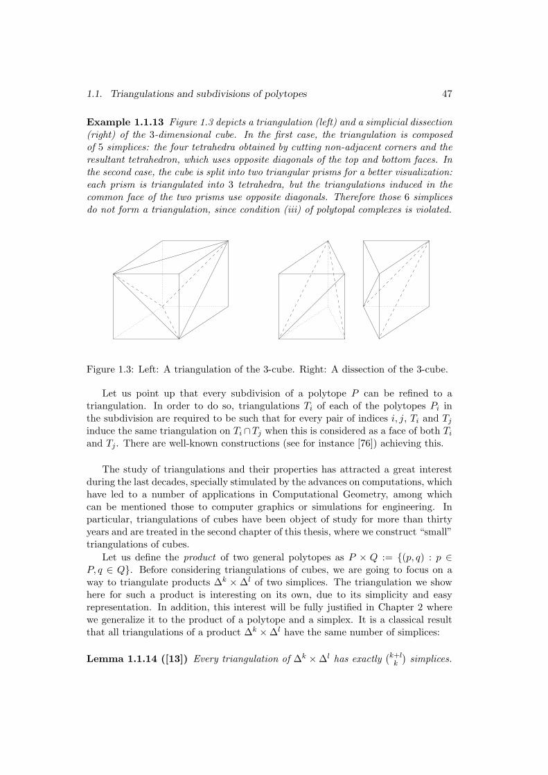
1.1. Triangulations and subdivisions of polytopes 47
Example 1.1.13 Figure 1.3 depicts a triangulation (left) and a simplicial dissection(right) of the 3-dimensional cube. In the first case, the triangulation is composedof 5 simplices: the four tetrahedra obtained by cutting non-adjacent corners and theresultant tetrahedron, which uses opposite diagonals of the top and bottom faces. Inthe second case, the cube is split into two triangular prisms for a better visualization:each prism is triangulated into 3 tetrahedra, but the triangulations induced in thecommon face of the two prisms use opposite diagonals. Therefore those 6 simplicesdo not form a triangulation, since condition (iii) of polytopal complexes is violated.
Figure 1.3: Left: A triangulation of the 3-cube. Right: A dissection of the 3-cube.
Let us point up that every subdivision of a polytope P can be refined to atriangulation. In order to do so, triangulations Ti of each of the polytopes Pi inthe subdivision are required to be such that for every pair of indices i, j, Ti and Tj
induce the same triangulation on Ti∩Tj when this is considered as a face of both Ti
and Tj . There are well-known constructions (see for instance [76]) achieving this.
The study of triangulations and their properties has attracted a great interestduring the last decades, specially stimulated by the advances on computations, whichhave led to a number of applications in Computational Geometry, among whichcan be mentioned those to computer graphics or simulations for engineering. Inparticular, triangulations of cubes have been object of study for more than thirtyyears and are treated in the second chapter of this thesis, where we construct “small”triangulations of cubes.
Let us define the product of two general polytopes as P × Q := (p, q) : p ∈P, q ∈ Q. Before considering triangulations of cubes, we are going to focus on away to triangulate products ∆k ×∆l of two simplices. The triangulation we showhere for such a product is interesting on its own, due to its simplicity and easyrepresentation. In addition, this interest will be fully justified in Chapter 2 wherewe generalize it to the product of a polytope and a simplex. It is a classical resultthat all triangulations of a product ∆k ×∆l have the same number of simplices:
Lemma 1.1.14 ([13]) Every triangulation of ∆k ×∆l has exactly(k+l
k
)simplices.

48 Chapter 1. Introduction and Preliminaries
Our aim here is to provide the reader with a remarkable triangulation of ∆k×∆l,known and used in algebraic topology [30] for a long time, and whose easy visual-ization makes it a good example of how helpful combinatorics can be in order tounderstand geometric structures in high dimensions. This utility is at the back-ground of the whole thesis, and may be even more explicit in Chapters 2 and 3.
Assume ∆k and ∆l having vertices v0, . . . , vk and w0, . . . , wl respectively.Then the product ∆k ×∆l has vertex set
(vi, wj) : 0 ≤ i ≤ k, 0 ≤ j ≤ l,
which can be represented as the squares of a (k + 1) × (l + 1) grid whose rowscorrespond to vertices of ∆k and whose columns represent vertices of ∆l. See Ex-ample 1.1.15.
Now, consider paths from the vertex (v0, w0) to the vertex (vk, wl) whose stepsincrease by one either the index of v or that of w. In the representation, if welabel rows and columns of the grid in such a way that (v0, w0) and (vk, wl) are thelower-left and upper-right corner squares respectively, those paths correspond tomonotone staircases, in which each step is a movement from a square either towardsthe next to the right or to the one inmediately above it. Each such path selects asubset of k + l + 1 vertices of ∆k ×∆l and it is not difficult to see that determinesa (k + l)-dimensional simplex.
The collection of simplices given by all those paths, represented by the collectionof all monotone staircases in the grid, forms a triangulation of ∆k × ∆l, which isknown as the staircase triangulation. Note that the number of possible such pathsor staircases is precisely
(k+lk
).
Example 1.1.15 The next figure shows the staircase triangulation of the triangularprism ∆1 × ∆2. In the top row the representation of its vertex set (vi, wj) : 0 ≤i ≤ 1, 0 ≤ j ≤ 2 as the squares of a 2× 3 grid is depicted. Below we show the threepossible staircases in this grid and the corresponding tetrahedra, which triangulate∆1 ×∆2.
We turn now our attention to the family of regular d-cubes Id := [0, 1]d, d ≥ 0:“Simple” triangulations of the regular d-cube have several applications, such assolving differential equations by finite element methods or calculating fixed points(see, for example, [72]). In particular, it has brought special attention both froma theoretical point of view and from an applied one to determine the smallest sizeof a triangulation of Id (see [51, Section 14.5.2] for a recent survey). Let us pointup that the general problem of computing the smallest triangulation of an arbitrarypolytope is NP-complete even when restricted to dimension 3, see [10].
Definition 1.1.16 The size of a triangulation (or simplicial dissection) T of thed-cube is its number of d-simplices |T |. The smallest size of triangulations of Id isusually denoted φd.

1.1. Triangulations and subdivisions of polytopes 49
0v
1v
0v
0v
1v
1v
1v
w0
w1
w2
w1
w2
w0 w
1
w2
w00
v )( , )( ,
)( ,
)( ,
)( ,
)( ,
1∆
2∆
Figure 1.4: The staircase triangulation of ∆1 ×∆2.
Definition 1.1.17 Given a d-simplex τ = conv(p1, . . . , pd+1), its volume is definedto be
vol(τ) := abs
(∣∣∣∣∣ p1 . . . pd+1
1 . . . 1
∣∣∣∣∣)
/d!
The minimum volume of a d-simplex using the vertices of Id is therefore 1/d!,and since that of the d-cube equals 1, the maximum size of a triangulation of Id turnsout to be d! A number of easily constructed triangulations achieving the maximumsize can be found in the above mentioned survey.
If we are given two triangulations of a d-cube for a fixed d, it is easy to decidewhich of them is “better” (or “simpler”); the one with smallest size. However, incase we have triangulations of d-cubes for different dimensions d, we need a notionto discern which of them is the most convenient. This was first stated by Todd in[72]:
Definition 1.1.18 The efficiency of a triangulation T of a d-cube is defined to bethe number (|T |/d!)1/d. The smallest efficiency (φd/d!)1/d of triangulations of Id isdenoted ρd.
Remark 1.1.19 By the above observation about the maximum size of a triangu-lation of the d-cube, the efficiency of a triangulation of Id is at most one and thesmaller it is, the most efficient is the triangulation. In particular, ρd ≤ 1,∀d.
In the second chapter of this thesis we present a new construction to triangulateId leading to asymptotically good efficiencies. That construction is inspired in thefollowing method due to Haiman [40]:

50 Chapter 1. Introduction and Preliminaries
Let Tk and Tl be triangulations of the regular cubes Ik and I l, respectively. Theproduct Tk × Tl of the two triangulations (understood as the pairwise product oftheir simplices) gives a decomposition of the cube Ik × I l = Ik+l into |Tk| · |Tl|subpolytopes, each of them isomorphic to the product of simplices ∆k × ∆l. ByLemma 1.1.14, every triangulation of ∆k × ∆l has size
(k+lk
). Hence, refining the
subdivision Tk × Tl in an arbitrary way one gets a triangulation of Ik+l of size|Tk| · |Tl| ·
(k+lk
), leading to:
Theorem 1.1.20 (Haiman) For every k and l, ρk+lk+l ≤ ρk
kρll.
The implication of this is that starting with a triangulation of a cube Ik of acertain efficiency ρ, one can construct a sequence of triangulations of Ink for n ∈ N
and with exactly that same efficiency. This inmediately suggests the following result:
Corollary 1.1.21 The sequence (ρn)n∈N
converges and
limn→∞
ρn ≤ ρd ∀d ∈ N.
Proof: Let us fix d ∈ N and k ∈ 1, . . . , d. Haiman’s theorem implies that, forevery i ∈ N,
ρk+id ≤ ρkk/(k+id)ρd
id/(k+id).
Since the right-hand side converges to ρd when i grows, the d subsequences of(ρn)
n∈Nconsisting of indices equal modulo d, and hence the whole sequence (ρn)
n∈N,
have upper limit bounded by ρd. This holds for every d ∈ N. An upper limit boundedby every term in the sequence must coincide with the lower limit.
We denote ρ∞ and call asymptotic efficiency of triangulations of the cube thelimit of (ρn)
n∈N. The corollary says that the asymptotic efficiency of triangulations
of the regular cube is at most the smallest effiency ρd for every d. In particular, thebest upper bound for ρ∞ prior to our work was ρ∞ ≤ ρ7 = 0.840. In Chapter 2 weprove ρ∞ ≤ 0.8159 with a completely novel method.
1.2 Graph Theory
Graph theorists agree to consider Euler’s paper [31] (in which the famous problemon the bridges of Konigsberg was discussed) to mark the birth of Graph Theory. Anumber of mathematicians have contributed since then to this field, but it has beenduring the last century when it has attracted a great interest, increased during thelast decades due to the simplicity of representing a graph on a computer and thebig number of problems that can be modeled using graphs.
In this section we first present some relations between graphs and polytopes; thefirst of them is the polytope of subdivisions of a convex polygon and is related tothe results of Chapter 3. The others are interesting properties of graphs defined byvertices and edges of polytopes. Finally, we state a result by Tutte about embed-dability of an abstract graph as a geometric one, with points of R
2 as vertices andstraight segments as edges.

1.2. Graph Theory 51
1.2.1 Preliminaries and relations with polytopes
The reader will be familiar with the basic notions we list here. For a general referenceon graphs we recommend [15] or [75], and for each statement in this section we specifywhere a proof can be found.
Definition 1.2.1 A graph is a pair of sets G = (V, E) where V = 1, . . . , n is afinite set of vertices and E ⊆ i, j : i, j ∈ V, i = j is a set of edges between thevertices. We will usually denote edges by ij instead of i, j.
By definition, the graphs we are considering are simple; they have neither loops(edges joining an element with itself) nor multiple edges. In the next definition wesummarize some basic vocabulary. By
(V2
)we denote the set of all unordered pairs
of vertices from V :
Definition 1.2.2 Let G = (V, E) be a graph.
• The number of edges in E containing a vertex v ∈ V is said to be the degreeof that vertex.
• G is regular of degree k if every vertex has degree k.
• G is complete if E =(V
2
). The complete graph on n vertices is denoted Kn.
• The graph obtained from G by the removal of a vertex set W ⊆ V is defined asthe restriction of G to the vertex set V \W , that is; G\W := (V \W, E∩
(V \W2
)).
• The set of neighbors of a vertex v is defined as N(v) := w ∈ V : v, w ∈ E.
• A graph G0 = (V0, E0) is a subgraph of G, denoted G0 ⊆ G, if V0 ⊆ V andE0 ⊆ E.
We consider three distinguished types of subgraphs:
• A path in G between two vertices v1, vk ∈ V (note that 1, k are subindicesand not necessarily vi = i) is a subgraph Gvk
v1⊆ G with vertex set V vk
v1=
v1, . . . , vk and edge set Evkv1
= v1, v2, v2, v3, . . . , vk−1, vk.
• A k-cycle in G is a subgraph Gv1v1⊆ G with V v1
v1= v1, . . . , vk and Ev1
v1=
v1, v2, v2, v3, . . . , vk−1, vk, vk, v1.
• A Y -graph in G of endpoints v1, v2, v3 ∈ V is a subgraph composed of a vertexw ∈ V \ v1, v2, v3 and paths Gw
v1, Gw
v2, Gw
v3which are disjoint except for the
common point w.
And a special type of graphs which will appear later:
• G is a bipartite graph if V is the disjoint union of two sets V1, V2 and each edgejoins a vertex of V1 to one of V2. It is said to be complete if its edges are allthe possible ones between V1 and V2. The complete bipartite graph is denotedKm,n, where m and n are the cardinalities of the subsets.

52 Chapter 1. Introduction and Preliminaries
Paths and cycles are often denoted by the sequence of appearance of vertices, thatis, (v1, v2, . . . , vk) or (v1, v2, . . . , vk, v1). Another notion which is of interest for us isthat of connectivity:
• G is connected if for any pair of distinct vertices v, w ∈ V there is a path Gwv
joining them.
• G is k-connected for k > 1 if for every v ∈ V the graph G\v is (k−1)-connected.
Thus, an abstract graph G = (V, E) is given as a set of vertices together witha set of unordered pairs of vertices, and no geometry is involved. On the otherhand, a topological embedding G → S
2 is a mapping of the vertices V to pointsin the 2-sphere and of the edges ij ∈ E to arcs. It is said to be a plane or non-crossing embedding if no pair of arcs pipj and pkpl corresponding to non-adjacentedges ij, kl ∈ E, i, j ∈ k, l has a point in common.
A geometric embedding, or geometric graph, G(S) = (V, E, S) is defined as agraph G = (V, E) together with a mapping i → pi ∈ S of the vertices V to a finiteset of points S := p1, . . . , pn ⊂ R
2 in the euclidean plane and of the edges ij ∈ Eto straight line segments pipj . Analogously, it is plane, or non-crossing, if no pair ofsegments corresponding to non-adjacent edges intersect. Fary’s Theorem [33] statesthat every plane topological embedding can be “stretched” to a plane geometricembedding. On the other hand, every plane geometric embedding trivially inducesa plane topological embedding (just projecting to S
2). A graph is said to be planarif it has a plane topological or geometric embedding.
The cells, or faces, of a plane geometric or topological embedding are definedto be the connected components of the complement (in R
2 or S2) of the union of
edges and vertices. A geometric embedding has exactly one unbounded face, usuallycalled outer face.
In this thesis we will consider only embeddings of graphs in R2 or S
2. We willuse the notations G(S) and G → S
2 for geometric and topological embeddings,respectively. But we may abuse notation and use the image set S to refer to thegeometric embedding G(S). The next result collects some useful statements; theirproofs can be found, for instance, in [77]:
Theorem 1.2.3 Let G be a graph.
(i) (Menger’s Theorem) G is k-connected if, and only if, between any pair ofvertices there are k paths G1, . . . , Gk in G which are disjoint except for theendpoints.
(ii) (Kuratowski’s Theorem) G is planar if, and only if, it has no subgraphhomeomorphic to the complete graph K5 or to the complete bipartite graphK3,3.
(iii) (Whitney’s Theorem) If G is planar and 3-connected, then all its topologicalembeddings are equivalent (have the same cells).

1.2. Graph Theory 53
(iv) (Euler’s Theorem) If G is connected and planar, for every plane embeddingG(S) (or G → S
2) the numbers c of cells, v of vertices and e of edges arerelated by
v − e + c = 2
Let us consider now the class of geometric non-crossing graphs on a given setof vertices A in the plane R
2. This type of graphs is of interest in ComputationalGeometry, Geometric Combinatorics, and related areas. In particular, much efforthas been directed towards enumeration, counting and optimization on the set ofmaximal such graphs, that is to say, triangulations. Note that here triangulationsare considered with set of vertices equal to A as advanced in Remark 1.1.12. Sinceany triangulation of a point set of cardinality n has ni + 2n − 3 edges for ni thenumber of points in the interior of conv(A), a lower bound of 2ni+2n−3 = Ω(4n) non-crossing graphs on A is trivial. An upper bound of type O(cn) for some constant cwas first shown in [5]. The best current value for c is 59 · 8 = 472 [62].
It is clear that the set of non-crossing geometric graphs on a planar point setforms a poset with respect to the inclusion of edges. However, until the developmentof this thesis their poset structure was only well understood if the points were inconvex position. The paper [34] contains several enumerative results about geometricgraphs with n vertices in convex position. In particular, it shows that there areΘ((6+4
√2)nn−3/2) non-crossing graphs in total and gives explicit formulas for each
fixed cardinality.For points in convex position the non-crossing graphs containing all the convex
hull edges are the same as the polygonal subdivisions of the convex n-gon. It iswell-known that the poset they form is the opposite of the face poset (except for theempty face) of the (n− 3)-associahedron, a simple polytope of dimension n− 3 withthe following properties:
• Its vertices correspond to all the 1n−1
(2n−4n−1
)different ways of bracketing a string
of length n−1 or, equivalently, of multiplying an expression a1a2 . . . an−1 whenmultiplication is not associative.
• Two vertices are adjacent if they correspond to a single application of theassociative law.
Thus, vertices of the associahedron correspond to polygonal subdivisions withthe maximal number of edges, i.e. triangulations.
Example 1.2.4 Figure 1.5 depicts the 2-associahedron (left), whose vertices corre-spond to all the 5 ways of bracketing the string 1234. Hence it is a pentagon, whoseface lattice we have already found in Figure 1.2. Neglecting the empty face, this ischecked to coincide with the opposite of the poset of polygonal subdivisions of theconvex 5-gon, which we show in the right picture.
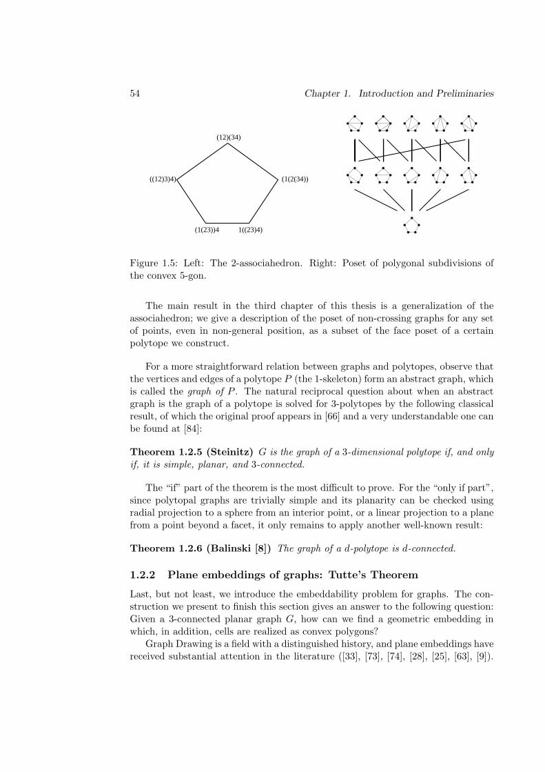
54 Chapter 1. Introduction and Preliminaries
(12)(34)
((12)3)4) (1(2(34))
(1(23))4 1((23)4)
Figure 1.5: Left: The 2-associahedron. Right: Poset of polygonal subdivisions ofthe convex 5-gon.
The main result in the third chapter of this thesis is a generalization of theassociahedron; we give a description of the poset of non-crossing graphs for any setof points, even in non-general position, as a subset of the face poset of a certainpolytope we construct.
For a more straightforward relation between graphs and polytopes, observe thatthe vertices and edges of a polytope P (the 1-skeleton) form an abstract graph, whichis called the graph of P . The natural reciprocal question about when an abstractgraph is the graph of a polytope is solved for 3-polytopes by the following classicalresult, of which the original proof appears in [66] and a very understandable one canbe found at [84]:
Theorem 1.2.5 (Steinitz) G is the graph of a 3-dimensional polytope if, and onlyif, it is simple, planar, and 3-connected.
The “if” part of the theorem is the most difficult to prove. For the “only if part”,since polytopal graphs are trivially simple and its planarity can be checked usingradial projection to a sphere from an interior point, or a linear projection to a planefrom a point beyond a facet, it only remains to apply another well-known result:
Theorem 1.2.6 (Balinski [8]) The graph of a d-polytope is d-connected.
1.2.2 Plane embeddings of graphs: Tutte’s Theorem
Last, but not least, we introduce the embeddability problem for graphs. The con-struction we present to finish this section gives an answer to the following question:Given a 3-connected planar graph G, how can we find a geometric embedding inwhich, in addition, cells are realized as convex polygons?
Graph Drawing is a field with a distinguished history, and plane embeddings havereceived substantial attention in the literature ([33], [73], [74], [28], [25], [63], [9]).

1.2. Graph Theory 55
Also, extensions of graph embeddings from straight-line to pseudo-line segments havebeen recently considered (see e.g. [55]). It is natural to ask which such embeddingsare stretchable, i.e. whether they can be realized with straight-line segments whilemaintaining some desired combinatorial substructure. Indeed, the primordial planargraph embedding result, the afore mentioned Fary’s Theorem [33], is just an instanceof answering such a question.
An explanation of the background of the following construction can be easilygiven by this physical fact: Assume that the edges of G are rubber bands. Takethe vertices corresponding to one particular cell F0 whose boundary has m vertices.Then, pin down these vertices in the plane R
2 in such a way that F0 is realized as aconvex m-gon and that all interior rubber bands are under tension. Voila; the figureobtained is a plane embedding of G in which all the remaining cells are realized asnon-overlapping convex polygons.
In order to model rubber bands, the notion of weight wij ∈ R of an edge ij isintroduced. Note that since we are considering non-directed edges, the symmetrycondition wij = wji has to be required.
Definition 1.2.7 Let G = (V, E) be a graph and w : E → R be an assignment ofweights to the edges. Consider also an assignment of positions i → pi ∈ R
2 for thevertices of G. A vertex i ∈ V is said to be in equilibrium if∑
ij∈E
wij(pi − pj) = 0.
See Figure 1.6 for an example.
The following important result gives a partial answer to the following question:When can a graph be embedded with straight edges in the plane, in such a waythat the cells are convex and do not overlap? (The latter is equivalent to “withoutcrossings”).
Theorem 1.2.8 (Tutte) Let G = (1, . . . n, E) be a 3-connected planar graph thathas a cell (k + 1, . . . , n) for some k < n. Let pk+1, . . . , pn be the vertices of a convex(n − k)-gon (in this order). Finally, let w : E′ → R
+ be an assignment of positiveweights to the internal edges. Then:
(i) There are unique positions p1, . . . , pk ∈ R2 for the interior vertices in such a
way that all of them are in equilibrium.
(ii) All cells of G are realized as non-overlapping convex polygons.
Although giving a whole proof of this result is out of the purposes of this intro-ductory chapter, we outline in the rest of this section the steps of the proof givenin [60], which we slightly modify in Chapter 4 to prove a directed version of Tutte’sTheorem. We include here the notions, intermediate results and proofs to which wewill refer in that chapter.

56 Chapter 1. Introduction and Preliminaries
Proof of (i): Assume that the positions of the boundary points pk+1, . . . , pn aregiven. Without loss of generality, we may assume pn = (0, 0). Consider the function
E(x1, . . . , xk, y1, . . . , yk) =12
∑ij∈E′
wij((xi−xj)2 +(yi−yj)2) =12
∑ij∈E′
wij‖pi−pj‖2,
which is quadratic and non-negative everywhere. Assume that the point z =(x1, . . . , xk, y1, . . . , yk) has at least one entry, say xl, with large absolute value. Thisimplies that pl is far away from the boundary point pn = (0, 0). Since the graph Gis connected, there is a path joining pl and pn; for at least one edge ij in this paththe distance ‖pi − pj‖ has to be large.
Thus, for sufficiently large α > 0, the condition |z| > α implies E(z) > E(0).Being E quadratic, this implies that it is strictly convex (non-degenerate with apositive definite Hessian) and therefore takes its unique minimum on z : |Z| < α.The assertion follows because the condition ∇E = 0 for a critical point of E:
∂E
∂xl=
∑ij∈E′
wij(xi − xj) = 0 and∂E
∂yl=
∑ij∈E′
wij(yi − yj) = 0, ∀l ∈ 1, . . . , k
is exactly the equilibrium condition for the interior vertices.
Sketch of the proof of (ii): Again, assume that the positions for the boundarypoints pk+1, . . . , pn are given; by (i) the positions for the interior vertices are inturn uniquely determined. Such a point configuration is called an equilibrium rep-resentation of G.
Example 1.2.9 In Figure 1.6 an equilibrium representation of a graph G, togetherwith the weights of each interior edge, is depicted. A grid is provided with the aimthat the reader can easily check the three interior vertices to be in equilibrium.
1 11
1 1
1
Figure 1.6: A graph in equilibrium.

1.2. Graph Theory 57
The relative interior of (the convex hull of) a collection of points S := p1, . . . , pn ⊂R
2 is defined by
relint(S) := n∑
i=1
λipi :n∑
i=1
λi = 1 and λi > 0, ∀i = 1, . . . , n.
Next lemma, whose proof is straightforward using the equilibrium condition,gives a property which turns out to be fundamental in Tutte’s Theorem. The state-ment can be checked again in Figure 1.6:
Lemma 1.2.10 In an equilibrium representation S := p1, . . . , pn ∈ R2n of the
vertices of G , every interior vertex p is in the relative interior of its neighbors;p ∈ relint(N(p)).
Definition 1.2.11 Let G be a 3-connected, planar graph on n vertices such thatthose labelled k + 1, . . . , n form, in this order, a cell of G. A point configurationS := p1, . . . , pn ∈ R
2n is said to be a good representation for G if:
(i) pk+1, . . . , pn realize, in this order, a convex (n− k)-gon, and
(ii) For i = 1, . . . , k we have pi ∈ relint(N(pi)).
Lemma 1.2.10 states that equilibrium representations are good representations.Tutte’s theorem then follows from this fact and the following assertion:
Theorem 1.2.12 ([60]) A good representation of a 3-connected planar graph G isa plane geometric embedding of G in which all interior cells are realized as non-overlaping convex polygons.
The proof is dissected into several smaller claims and has two different parts. Inthe first one, the following lemma proves that degenerate situations cannot occur,where a vertex pi is said to be degenerate if the set of its neighbors N(pi) doesnot affinely span R
2. Its proof can be skipped in a first reading and, as advancedabove, appears here for a better understanding of the differences with the proof ofthe directed Tutte Theorem given in Chapter 4:
Lemma 1.2.13 ([60]) A good representation S of a 3-connected planar graph Ghas no degenerate vertices.
Proof: Before starting the proof, given a line 3 = x : φ(x) = α for φ a linearfunctional, a vertex a is defined to be 3-active if not all its neighbors are also on 3.
It is straightforward that the boundary points are non-degenerate, since theyare the vertices of an strictly convex polygon. Consider then a degenerate interiorvertex p ∈ S, for which there must be a line 3 = x : φ(x) = α such that p ∈ 3 andN(p) ⊂ 3.

58 Chapter 1. Introduction and Preliminaries
Take a point q ∈ S which is not on 3. Since G is 3-connected, Menger’s Theorem1.2.3.(i) guarantees the existence of three paths A, B, C from p to q having disjointedges and vertices, except for the endpoints p, q. Since each of them has to leavethe line 3 at some point, they contain at least one 3-active vertex each. Denote bya the first 3-active point coming after p in the path A. The initial segment of thispath is then of the form A0 = (p, a1, . . . , al, a) and all its points are on 3. Denote byb and c the first 3-active points coming after p respectively in B and C. Likewise,let B0 and C0 be the corresponding initial segments. Observe that, all together, theedges of A0, B0 and C0 form a Y -graph with endpoints a, b, c, denoted Y 0, which iscontained on 3.
The next step is to prove that there are also Y -graphs Y + and Y − having thesame endpoints a, b, c and whose edges are all respectively above and below the line3. Only the existence of Y + is shown, since that of Y − is proved analogously:
At most two of the boundary vertices can lie on 3, therefore among the pointsa, b, c there are at most two boundary points. Assume that a is interior. For anyinterior point q ∈ S the definition of good representation implies q ∈ relint(N(q)),what implies in turn the following property:
If there is a q− ∈ N(q) with φ(q) > φ(q−),then there is also a q+ ∈ N(q) with φ(q) < φ(q+)
which holds as well for boundary points that are not maximal with respect to φ.Being a an 3-active point, there is either a point a+ ∈ N(a) with φ(a) < φ(a+) ora point a− ∈ N(a) with φ(a) > φ(a−), in which case the previous property impliesthe existence of an a+ ∈ N(a) with φ(a) < φ(a+), too.
Iterating, a path A+ = (a+0 , . . . , a+
l ) connecting a = a+0 with a boundary point
a+l = a+ maximal with respect to φ can be generated. Analogously, paths B+ and
C+ from b and c to φ-maximal boundary points b+ and c+ are constructed.Since there are at most two such φ-maximal boundary points, either a+ = b+ =
c+ or they correspond to two points connected by an edge. Consider now the sub-graph G+ of G containing the paths A+, B+, C+, which is connected. In addition,the three 3-active vertices a, b, c have degree one in G+. Thus, the component G+
contains a Y -graph Y + of endpoints a, b, c having all edges above 3. Similarly, thereis a Y -graph Y − with the same endpoints and all edges below 3.
Hence, there are three edge-disjoint Y -graphs, namely Y 0, Y + and Y −, havingendpoints a, b and c: They form a subgraph homeomorphic to the complete bipartitegraph K3,3, what contradicts the planarity of G by Theorem 1.2.3.(ii).
For the second part of the proof of Theorem 1.2.12, a global consistency argu-ment given by a series of claims that we do not list here (we refer the reader to [60]),is used in order to show that all the cells are indeed convex and non-overlapping.

1.3. Rigidity Theory 59
1.3 Rigidity Theory
It was again Euler who in 1766 conjectured “A closed spatial figure allows no changes,as long as it is not ripped apart” [32], setting the starting point of Rigidity Theory.However, the first major published result [18] is attributed to Cauchy in 1813: thegraph of every simplicial 3-polytope is rigid. This was a first step towards thestudy of Euler’s Conjecture, which was finally disproved in 1978 by R. Connelly[21]. Another notorious contribution to the history of rigidity are the works of J.C.Maxwell [52], who studied stresses and forces on graphs and their relations withreciprocal figures.
Although results in Rigidity Theory have been rather sparse from the statementof Euler’s conjecture to its resolution, since the 1970s a huge number of researchershave directed their efforts to this field, leading to a number of engineering applica-tions, see for example [42]. Techniques from Rigidity Theory have also been recentlyapplied to answering long-standing problems from robotics or molecular modelling([22], [69], [12]). Work on understanding some fundamental geometric propertiesof molecular conformations is currently approached via such techniques [47], withpotential applications in protein folding [82], [71].
In this chapter we first give a series of notions and facts, before giving a relationbetween forces and reciprocal figures which will appear later in our results. Then wegive the definition of generic infinitesimal rigidity, which is the fundamental notionfor us, and finally we present the graphs with the property of being minimal amongthose infinitesimally rigid and sketch how they can be constructed. We mainlyconsider geometric embeddings, although topological embeddings will also appearin Subsection 1.3.2.
1.3.1 The rigidity matrix
A particular geometric embedding G(S) = (V, E, S) of a graph G = (V, E) is usuallycalled a framework when referring to its rigidity properties. The complete frameworkfor a point set V is that having the complete set K =
(V2
)of edges. As observed
before, troughout this thesis we will consider geometric embeddings only into R2,
although most of this section holds for embeddings into a general Rm as well. In
the affine plane (and in the 3-dimensional space), one may think of a framework as amathematical model for a physical structure in which each vertex i corresponds to aball joint located at the point pi and each edge corresponds to a rigid rod connectingthe joints at its endpoints.
Obviously, this representation may be used to describe equally rigid structures(like bridges) as moving ones (like machines or organic molecules). Dealing with thedistinction between frameworks whose realization is rigid and those which admitmovements is the goal of the Rigidity Theory. At a first step, it would be expectedthat a framework being or not rigid depends both on the graph G = (V, E) and theparticular embedding G(S), what makes the difference between the combinatorialand the geometric rigidity. In the rest of the section our goal is to minimize the

60 Chapter 1. Introduction and Preliminaries
importance of the particular embedding and focus mainly on the graph properties.With this aim, we introduce the basic notions needed to understand the resultsabout rigidity presented in the following chapters. Unless otherwise said, for theresults in this section we refer the reader to [38].
Definition 1.3.1 Let G(S) be an embedding of a graph G on a finite set of pointsS := p1, . . . , pn ⊂ R
2. The set S is in general position and G(S) is a generalembedding if no 3-subset of S lies on a line.
If we identify an embedding G(S) on the set S := p1, . . . , pn ⊂ R2 with a point
S = (p1, . . . , pn) ∈ R2n, we can measure lenghts of edges by the rigidity function
r : R2n → R
(n2)
S → r(S)ij := ‖pi − pj‖2
which is continuosly differentiable. Then, the rigidity matrix R(S) of the embeddingG(S) is defined by r′(S) = 2R(S). It is an
(n2
)× 2n matrix with condensed form
R(S) =
p1 − p2 p2 − p1 0 0 . . . 0 0p1 − p3 0 p3 − p1 0 . . . 0 0
......
......
. . ....
...0 0 0 0 . . . pn−1 − pn pn − pn−1
We are going to introduce a crucial notion in terms of rows of the rigidity matrix.
Recall that these correspond to pairs of vertices and then to edges of the completegraph on V :
Definition 1.3.2 A set of edges E ⊆(V
2
)is said to be independent with respect to
an embedding S if the corresponding rows in the rigidity matrix are independent.
Let δ(S) denote the determinant of some |E|×|E|minor of the submatrix definedby E. If we permit S to vary over all points in R
2n, the solution set to δ(S) = 0is either all of R
2n or an algebraic hypersurface. The latter is the case if there isan embedding S with respect to which E is independent. Then, the set of all em-beddings S for which rows corresponding to E are dependent lies in the intersectionXE of the algebraic hypersurfaces corresponding to all the |E| × |E| minors of thesubmatrix. If E is independent with respect to some embedding, each XE is a closedalgebraic set of measure zero.
Definition 1.3.3 An embedding S is said to be generic if S ∈ X , where
X = ∪XE : E independent for some embedding.
Observe that X is a closed set of measure zero in R2n.
Definition 1.3.4 An edge set E ⊆(V
2
)is generically independent if it is indepen-
dent with respect to all generic embeddings of V .

1.3. Rigidity Theory 61
This definition, together with that of generic embeddings, makes the followingresult straightforward:
Lemma 1.3.5 Let V be a finite set of vertices. If a set of edges E ⊆(V
2
)is inde-
pendent with respect to some embedding of V , then it is generically independent.
We now observe that for a particular embedding S and a set E of edges, con-sidering the minors of the set of rows of R(S) which correspond to E is not a verypractical way of checking independence. Instead, one usually looks directly at thedependency relations between rows of the rigidity matrix:∑
ij∈E
wijrij = 0,
for rij the row corresponding to the edge ij. A set of edges E is independent withrespect to the embedding S if, and only if, the only dependency relation satisfied bythe corresponding set of rows is the trivial one (that with wij = 0 for all ij).
Definition 1.3.6 A non-zero stress on a framework G(S) is an assignment of scalarswij , not all zero, to the edges E of G in such a way that, for every vertex i ∈ V ,∑
ij∈E
wij(pi − pj) = 0.
For a physical interpretation, the assignment of wij ’s may correspond to thereplacement of each edge ij with a spring whose compression or extension is indicatedby the value wij . Note that the last expression is just the previous one consideredone column at a time. Then, with respect to the embedding S, a set of edgesbeing independent, that is, their rows in the rigidity matrix having only the trivialdependency, is equivalent to those edges having only the trivial stress.
A graph is said to have a stress (sometimes called self-stress) if its edges haveit on any generic embedding. Analogously, a graph is a generic rigidity circuit iffor any generic embedding its edges have a non-zero stress but no proper subset ofedges has one. In other words, a circuit is a minimal dependent set of rows in therigidity matrix of any generic embedding. Hence, a framework G(S) is a rigiditycircuit precisely if it has a unique stress and the stress is not zero on any edge.
Example 1.3.7 The reader may have noticed that, given an embedding G(S) of agraph, having a stress on the edges is equivalent to every vertex (including boundaryones) being in equilibrium with its neighbors. The difference with the situation inTutte’s Theorem is that we now allow negative weights on edges.
In the next figure we add weights of boundary edges of Figure 1.6. It can be easilychecked that the three boundary points are also in equilibrium.

62 Chapter 1. Introduction and Preliminaries
1 11
1 1
1
-1/4 -1/4
-1/4
Figure 1.7: A stress in the graph of Figure 1.6.
1.3.2 Stresses and reciprocal graphs
Roughly speaking, in this subsection we show that for those frameworks with stressessuch that wij = 0 for every edge ij, a dual can always be drawn with an interestinggeometric property. In order to do so, we first need a few notions:
Definition 1.3.8 A spherical framework is defined to be a pair (G → S2, G(S))
composed of a plane topological embedding G → S2 and a (possibly not plane)
geometric embedding G(S), of a graph G.A non-crossing spherical framework is a plane geometric embedding G(S) to-
gether with its trivially corresponding plane topological embedding G → S2 (the
one given by the inclusion R2 → S
2).
Definition 1.3.9 Given a plane topological embedding G → S2 of a 2-connected
graph G = (V, E), the set E of its edge patches is defined to have as elements theordered 4-tuples e = (i, j;h, k) such that the edge from vertex i to vertex j has faceh on the right and face k on the left.
Of course, the definition holds as well for plane geometric embeddings; actuallywe refer the reader to Figure 1.8 (left) in order to check the notion of edge patch.There, edges are denoted by numbers and faces by letters. However, we are goingto use this definition in the context of spherical frameworks, where planarity is onlyguaranteed for the topological embedding.
Definition 1.3.10 • The dual G′ → S2 of a plane topological embedding G → S
2
was introduced by Poincare and is the cell decomposition of S2 having one ver-
tex for each cell of G and in which two vertices are joined by an edge if thecorresponding cells are adjacent in G. Observe that the dual of an edge patche = (i, j;h, k) is e′ = (h, k; j, i).

1.3. Rigidity Theory 63
• A spherical framework (G′ → S2, G′(S′)) is a reciprocal of a spherical frame-
work (G → S2, G(S)) if G′ → S
2 is the dual of G → S2 and for each edge
patch (i, j;h, k) ∈ E,〈pi − pj , p
′h − p′k〉 = 0.
That is to say, the edges of the geometric embeddings G(S) and G′(S′) areperpendicular.
Figure 1.8 shows the geometric embeddings G(S) (left) and G′(S′) (right) ofa non-crossing spherical framework and its reciprocal. The points a, . . . , d in theoriginal represent faces.
21
3
4
b
a
d c
21
3
4
d c
b
a
Figure 1.8: Reciprocal geometric embeddings.
Note that the dual of a plane topological embedding always exists. Hence, givena spherical framework, the non-trivial part in the definition of reciprocal is theexistence of G′(S′). This is why in the next result we abuse of the notation andomit the topological part of spherical frameworks:
Theorem 1.3.11 (Maxwell-Cremona) For a spherical framework G(S), the fol-lowing are equivalent:
(i) G(S) has a reciprocal G′(S′),
(ii) G(S) has a stress∑
ij∈E wij(pi− pj) = 0 such that wij = 0,∀ij ∈ E (non-zeroon all edges).
(iii) There is a piecewise-linear lifting (may be non-convex and self-intersecting) ofG(S) into 3 dimensions, linear on every face.
Furthermore, if the conditions hold for G(S):

64 Chapter 1. Introduction and Preliminaries
• Edges with positive/negative stress correspond to valleys/ridges in the liftingof (iii). (Meaning that the slope increases/decreases when crossing the edge).
• The conditions also hold for the reciprocal G′(S′).
Proof: We will refer to the equivalence (i)⇔(ii), appeared in [52], as Maxwell’sTheorem. We give here its proof, which will be crucial in Chapter 5. For that of theequivalence to the third condition see [24], [43] or [78]. Note that the two sides of avalley (resp. ridge) do not necessarily “go up” (resp. “go down”).
(ii)⇒(i) Assume that there is such a stress. Choose an initial point p′0 for the re-ciprocal corresponding to a cell F0 of the original, and define the point correspondingto another cell Fc by p′c = p′0 + (
∑e′ wede)⊥ where the sum is over the edge patches
e′ = (h, k; j, i) of any path from F0 to Fc in the dual graph, and where de = pj − pi.Observe that this is an inductive process for which the intermediate points betweenp′0 and p′k have been previously obtained. The first task is to prove that, given anytwo such paths between F0 and Fc, both lead to the same p′c, what is true since thesum up one path and back the other follows a sum of face cycles, and each face cycleis zero by the equilibrium condition on its reciprocal vertex. Since no wij is zero,there is no degenerate edge in the reciprocal.
(i)⇒(ii) Given a reciprocal, the previous construction can be reversed, solvingthe system (wede)⊥ = p′k − p′h to get back the unique corresponding stress in theoriginal framework. Since the vector sum of edges in every face cycle is zero, thevertices of the original are in equilibrium.
Observation 1.3.12 Let G′(S′) be the reciprocal of G(S) obtained from a certainstress of weights wij . Let e = (i, j;h, k) denote an edge patch in the original, then:
• p′k − p′h = wij(pj − pi)⊥. That is; the straight segment in the reciprocalis perpendicular to the corresponding in the original, scaled by the absolutevalue of the stress and with direction given by the sign.
• G′(S′) has a stress non-zero on all edges defined as w′hk := 1/wij .
Example 1.3.13 In Figure 1.8 the positions of a, . . . , d in the reciprocal (right)are obtained according to the previous proof, once defined in the original the stressw14 = w24 = w34 = 1 for interior and w12 = w23 = w13 = −1/3 for exterior edges.Observe that in the reciprocal the point a corresponding to the exterior face turnsout to be above b, what corresponds to the edge 12 having negative stress.
Remark 1.3.14 Even for non-crossing spherical frameworks, Maxwell’s Theorem1.3.11 only claims the existence of a reciprocal spherical framework, which is notguaranteed to be non-crossing. In Chapter 5 we characterize the conditions fornon-crossing spherical frameworks to have a non-crossing reciprocal.

1.3. Rigidity Theory 65
1.3.3 Infinitesimal rigidity and isostatic graphs
In this subsection we present the notion of rigidity we will use in this thesis and anoutstanding type of graphs, which are considered to be the fundamental objects in2-dimensional Rigidity Theory. We focus again on geometric embeddings.
Definition 1.3.15 Let G(S) = (1, . . . , n, E, S) be a framework and consider anassignment of a 2-dimensional vector vi to each vertex i. Such an assignment v ∈ R
2n
is said to be an infinitesimal motion of the framework if the following homogeneousequation holds for every edge ij ∈ E:
〈vi − vj , pi − pj〉 = 0.
The set of infinitesimal motions of such a framework is denoted V(E) and is clearlya linear subspace of R
2n.
Each vi can be interpreted as a velocity vector for the point pi in the plane.Infinitesimal motions are sometimes called flexes in the rigidity literature. For aninterpretation, consider the vector assignment v as the initial velocities of a mo-tion for the points pi, such that they neither compress nor strecht the rods of theframework. This is why a vector v such that
〈vi − vj , pi − pj〉 ≥ 0,
that is, such that it increases or keeps the length of the rods, is said to be anexpansive infinitesimal motion.
Here comes the precise definition of rigidity we are interested in:
Definition 1.3.16 A framework G(S) = (1, . . . , n, E, S) is said to be infinitesi-mally rigid if V(E) equals the subspace V(K) of infinitesimal motions of the completeframework G(K), which are the translations or rotations of the whole graph.
A graph G is generically infinitesimally rigid if it is infinitesimally rigid for everygeneric embedding S.
Lemma 1.3.17 ([38]) If G(S) is infinitesimally rigid for some general embeddingS of V , then the graph G is generically infinitesimally rigid.
In the sequel we focus on infinitesimal rigidity in the generic sense and, when re-ferring to a graph as “infinitesimally rigid”, we will mean “generically infinitesimallyrigid”. A graph G = (V, E) is said to be isostatic or minimally (infinitesimally) rigidif it is (infinitesimally) rigid and its edge set E is independent. Infinitesimal rigidityis then linear algebra, with infinitesimally rigid graphs, stresses and isostatic graphscorresponding to spanning sets, linear dependencies and bases of the row space ofthe rigidity matrix of the complete graph.
Let us observe that, for each edge ij, the condition 〈vi−vj , pi−pj〉 = 0 determinesa hyperplane in R
2n; that of the vectors v which keep the length of the rod pipj .

66 Chapter 1. Introduction and Preliminaries
Therefore, a hyperplane arrangement is associated to each framework via its edges.Orienting the hyperplanes according to whether the rods are stretched or shrunkdetermines the so-called rigidity matroid.
To finish the present section, we consider the following type of graphs, whichprovide a combinatorial characterization of infinitesimal rigidity:
Definition 1.3.18 A graph G = (V, E) is said to be Laman if the following condi-tions hold:
(i) |E| = 2|V | − 3, and
(ii) For every subgraph (V ′, E′) with |V ′| ≥ 2 vertices, |E′| ≤ 2|V ′| − 3.
Condition (ii), which is sometimes called the hereditary Laman property, can beequivalently restated as:
(ii’) Every subset V ′′ of vertices with |V ′′| ≤ |V | − 2 is incident to at least 2|V ′′|edges.
There is a variety of ways to characterize Laman graphs. The one we are mostinterested in for the purposes of this thesis, since a combinatorial version will be givenin Chapter 4, is the Henneberg construction [41]. It goes inductively as follows: Fora Laman (abstract) graph on n vertices, start with a triangle for n = 3. At eachstep, a new vertex is added in one of the following two ways:
• Henneberg I (vertex addition): The new vertex is connected via two edgesto two of the old vertices.
• Henneberg II (edge splitting): A new vertex is added on some edge, splittingthis into two new edges, and then connected to a third vertex. Equivalently,an edge is removed and then a new vertex is connected to its endpoints andto some other vertex.
1
3
2
5
4
5
6
4 2
1
3
Figure 1.9: Henneberg steps.

1.4. Pseudo-triangulations of convex bodies and points 67
Example 1.3.19 See Figure 1.9 for an example: The points have been added ac-cording to their labels and faces obtained previously to the current step are shaded. Inthe right picture we have chosen a drawing with crossing edges, in order to emphasizethat the Henneberg construction holds for general and not only planar graphs.
The next result shows that Laman graphs are the maximal independent sets,and justifies why they are fundamental in 2-dimensional Rigidity Theory. See [50],[38], [80]:
Lemma 1.3.20 ([81]) Let G = (V, E) be a graph with |V | ≥ 2. Then, the followingare equivalent:
(i) G is isostatic,
(ii) G is infinitesimally rigid with |E| = 2|V | − 3,
(iii) G is independent with |E| = 2|V | − 3,
(iv) G is a Laman graph (Laman’s Theorem, [50]),
(v) There is a Henneberg construction for G (Henneberg’s Theorem, [41]).
In order to conclude this section about rigidity, we include here the followingresult relating rigidity to polytopes via their graphs. For d = 3 it was proved byDehn [29] in 1916, and the generalization to d > 3 is due to Whiteley [79]:
Theorem 1.3.21 The graph of a simplicial d-polytope P is infinitesimally rigid.
Let us mention that the d = 3 case is an inmediate consequence of the theoremstated by Cauchy [18] in 1813 which we mentioned at the beginning of the section,whose proof turned out to have several minor errors and was completed later (see[67]).
1.4 Pseudo-triangulations of convex bodies and points
Pseudo-triangulations are relatively new objects which have by now been used inmany Computational Geometry applications, among them visibility [56, 58, 57, 65],ray shooting [37], kinetic data structures [1, 49] and motion planning for robotarms [69]. In this last paper, Streinu introduced the minimum or pointed pseudo-triangulations and used them to prove the Carpenter’s Rule Theorem (the first proofof which was given shortly before by Connelly et al. [22]).
They have rich combinatorial, rigidity theoretic and polyhedral properties, manyof which have only recently started to be investigated, see also [61], [59], [48], [3],[11], [2], [17]. Finding their 3-dimensional counterpart, which is perhaps the mainopen question about pseudo-triangulations and expansive motions, may lead to effi-cient motion planning algorithms for certain classes of 3-dimensional linkages, with

68 Chapter 1. Introduction and Preliminaries
potential impact on understanding protein folding processes. We introduce pseudo-triangulations in the context of visibility between convex bodies, where they orig-inally appeared, before turning our attention to pseudo-triangulations of points,those in which we will focus in this thesis.
1.4.1 Pseudo-triangulations of convex bodies
Although in this work we are not dealing with this type of pseudo-triangulations,their importance comes from the fact that precisely in this context Pocchiola andVegter started the study of pseudo-triangulations in the seminal papers [56] and[57], in which the results of this subsection can be found. A precedent appears inthe geodesic triangulations of polygons introduced in [19].
Pocchiola and Vegter consider a collection O = B1, . . . , Bn of pairwise disjointconvex bodies in the plane, which are assumed to be strictly convex (meaning thatthe open line segment joining any two points lies in the interior of the object), tohave a smooth C1-differentiable boundary and to be in general position in the sensethat no three objects share a common tangent line. The following definition collectsmost of the notions needed in this subsection, and can be checked in Figure 1.10:
Definition 1.4.1 In the situation above,
• A bitangent for a pair of convex bodies is a line segment which is tangentto the two objects at its endpoints, in the sense that the line containing thatsegment is locally a supporting line. There are four such bitangents; two whichseparate the objects and two which do not.
• The set of bitangents of a collection O = B1, . . . , Bn of pairwise disjointconvex bodies is composed of those line segments which are bitangents ofsome pair of the objects and do not intersect the others. It is called thetangent visibility graph.
• A pseudo-triangulation of O = B1, . . . , Bn is the subdivision of the planeinduced by a maximal (with respect to the inclusion) family of pairwise non-crossing bitangents of O.
Lemma 1.4.2 Every pseudo-triangulation of n convex bodies in general positionsubdivides conv(∪iBi) \ ∪iBi into 2n − 2 cells, and the number of bitangents is3n− 3.
The goal of Pocchiola and Vegter was the study of the tangent visibility graph ofa collection O of n convex bodies. In particular, they used pseudo-triangulations toobtain the first algorithm which constructs the graph in optimal time, O(n log(n)+k)(for k the graph size), using only linear space O(n). In their algorithm, the pseudo-triangulations counterpart of the well-known notion of diagonal flip in triangulations(see, for example [46]) turned out to be crucial:

1.4. Pseudo-triangulations of convex bodies and points 69
Figure 1.10: Flip between two pseudo-triangulations of a family of convex bodies.
Lemma 1.4.3 Any two disjoint cells T and T ′ have exactly one common tangentline. Furthermore, the removal of an interior bitangent gives a cell which can besplit in exactly another way by adding a different bitangent. This operation is calledflip.
An example of flip can be found between the dashed edges in Figure 1.10.
Corollary 1.4.4 From the two previous Lemmas, every pseudo-triangulation of Ohas exactly 3n− 3− nb flips, where nb is the number of bitangents in the boundaryof conv(∪iBi).
Thus, the graph of pseudo-triangulations of O, having pseudo-triangulations asvertices and flips as edges, is regular of degree 3n − 3 − nb. Pocchiola and Vegtershow that, in addition, it is connected.
1.4.2 Pseudo-triangulations of points
Consider a set A of n points in general position in the plane (one of the consequencesof the results in Chapter 4 is a natural definition of pseudo-triangulations in presenceof collinearities as well). A triangulation of A is a subdivision of the polygon conv(A)into triangles, in the sense of Remark 1.1.12, assuming that all the points of A areused as vertices.
Definition 1.4.5 Let us call convex and reflex angles those respectively smallerand greater than π and observe that the general position assumption implies theabsence of angles equal to π.
A pseudo-triangle is a simple polygon with only three convex vertices (from theinterior), called corners and joined by three inward convex polygonal chains, calledpseudo-edges of the pseudo-triangle. See Figure 1.11.(a).

70 Chapter 1. Introduction and Preliminaries
More generally, a pseudo-quadrilateral, pseudo-pentagon, etc. is a simple polygonwith exactly four, five, etc. convex vertices. For them a diagonal is defined asa segment contained in the pseudo-polygon and tangent to its boundary at theendpoints. Note that every convex k-gon is a pseudo-k-gon. In particular, everytriangle is a pseudo-triangle. Note also that every (perhaps non-convex) polygon isa pseudo-k-gon for some k.
A pseudo-triangulation of A is a geometric non-crossing graph with vertex setA and which partitions conv(A) into pseudo-triangles. Every triangulation is apseudo-triangulation.
(a) (b) (c)
Figure 1.11: (a) A pseudo-triangle. (b) A pointed pseudo-triangulation. (c) Thedashed edge in (b) is flipped, giving another pointed pseudo-triangulation.
Since triangulations of A coincide with the maximal non-crossing graphs on A,they are also the maximal pseudo-triangulations. As is well-known, they all have2nv + 3ni − 3 edges, where nv and ni denote the numbers of points of A in theboundary and interior of conv(A), respectively. It turns out that also the pseudo-triangulations with the minimum possible number of edges are very interesting fromdifferent points of view:
Definition 1.4.6 A vertex of a geometric graph is called pointed if its incidentedges span an angle smaller than 180 degrees from that vertex. The graph itself iscalled pointed if all its vertices are pointed.
A pointed pseudo-triangulation is that on which every vertex is pointed.
The following statement comes originally from [69]. We sketch here its proof,which can also be found in [61].
Proposition 1.4.7 (Streinu) Let A be a planar point set as above. Then:
(i) Every pseudo-triangulation of A with nγ non-pointed vertices and nε pointedvertices has 2n − 3 + nγ = 3n − 3 − nε edges and n − 2 + nγ = 2n − 2 − nε
pseudo-triangles.
(ii) Every pointed and non-crossing graph on A has at most 2n − 3 edges, and iscontained in some pointed pseudo-triangulation of A.

1.4. Pseudo-triangulations of convex bodies and points 71
Proof: The first part comes from Euler’s formula, which if we call t and e thenumbers of pseudo-triangles and edges, respectively, gives n − e + t = 1. We aregoing to obtain an additional formula by double-counting of the number of convexangles: On the one hand, each of the pseudo-triangles produces exactly three ofthem. On the other, for each non-pointed vertex there are as many convex anglesas incident edges, and for each pointed vertex the number of convex angles is oneless than that. Thus, 2e−nε = 3t and the formula above gives the desired values ofe and t.
For the second part, we first observe that we can assume the graph to be con-nected, since otherwise their components can be analyzed separately. Pointednessmeans that the number of reflex angles is n. The number of convex angles is at least3t, with equality if, and only if, the graph is a pseudo-triangulation. Since the totalnumber of angles sums up to 2e, we get 2e ≥ n + 3t which together with Euler’sformula implies e ≤ 2n−3 (and t ≤ n−2). The last sentence in the statement comesthen from two facts: On the one hand, that the addition of geodesic paths (thosenon-crossing paths having shortest length among paths sufficiently close to them)between convex vertices of a polygon keeps the graph pointed and non-crossing, andon the other the fact that there is always some geodesic path through the interiorof a polygon if this is not a pseudo-triangle.
Remarks 1.4.8 Observe that every vertex on the convex hull of A is triviallypointed. Then, the number nε of pointed vertices in a pseudo-triangulation runsfrom nv, in which case all the pseudo-triangles are indeed triangles and the pseudo-triangulation is actually a triangulation, to n for a pointed pseudo-triangulation.
Part (i) implies that, among pseudo-triangulations of A, pointed ones have theminimum possible number of edges. For this reason they are also called minimumpseudo-triangulations.
Part (ii) says that pointed pseudo-triangulations coincide with maximal non-crossing and pointed graphs.
Given a planar point configuration A, it is easy to construct a pointed pseudo-triangulation of it as follows: First, order the points of A according to their x-coordinate. Then, consider the triangle defined by the three starting points inthe ordering. Finally, add iteratively the two tangents joining each new point tothe previously constructed pseudo-triangulation. See Figure 1.12. Corollary 1.4.10below will show that it is not a coincidence that this procedure is a particular caseof a Henneberg construction.
Note that a minimum (i.e. pointed) pseudo-triangulation is always “minimal”in the sense that the removal of any edge implies we no longer have a pseudo-triangulation. However, minimal pseudo-triangulations need not be pointed. Foran example, consider Figure 1.13; the leftmost pseudo-triangulation is minimum(therefore minimal), the middle one is minimal but not minimum and the rightmostis not minimal and thus neither minimum.

72 Chapter 1. Introduction and Preliminaries
1
2
3
4
5
7
6
Figure 1.12: Construction of a pointed pseudo-triangulation.
Figure 1.13: Minimum, minimal and not minimal pseudo-triangulations.
The following result, taken from [69], summarizes the above characterizations ofpointed pseudo-triangulations and introduces a new one relating them to rigidity:
Theorem 1.4.9 (Characterization of pointed pseudo-triangulations)Let G = (V, E) a graph embedded on the point set A = p1, . . . , pn ⊆ R
2. Then,the following properties are equivalent:
(i) G is a pointed pseudo-triangulation,
(ii) G is a pseudo-triangulation and |E| = 2n − 3 (equivalently, the number ofpseudo-triangles is n− 2),
(iii) G is a minimum pseudo-triangulation, that is, it has the minimum number ofedges (equivalently, of pseudo-triangles) among all pseudo-triangulations of A.
Moreover, if any of the above conditions is satisfied, then G fulfills the hereditaryLaman property; for every subgraph (V ′, E′) with |V ′| ≥ 2 vertices, |E′| ≤ 2|V ′| − 3.
Proof: (i)⇔(ii)⇔(iii) follow from part (i) of Proposition 1.4.7. The Laman propertyfollows from part (ii) of the same result.
Corollary 1.4.10 (Streinu) Pointed pseudo-triangulations are Laman graphs, there-fore isostatic.

1.5. Results and Open problems 73
In particular, the fact that in addition to be Laman graphs, pointed pseudo-triangulations when stripped of a convex hull edge become expansive mechanisms[69], has proved to be crucial in designing efficient motion planning algorithms forplanar robot arms.
1.5 Results and Open problems
According to the problems studied, this thesis can be divided into two parts: Thefirst one deals with the problem of finding efficient triangulations of the hypercubeand is carried out in Chapter 2. The rest of the thesis, Chapters 3 to 5, is devoted tothe study of planar graphs, pseudo-triangulations and their relations with rigidity.Since the techniques we use are different, both parts can be regarded separately,although the two of them are framed in the context of Geometric Combinatorics.
1.5.1 Efficient triangulations of cubes
Once known a triangulation of efficiency ρ of a certain cube, Haiman’s constructiongives triangulations of size ρnn! of high-dimensional cubes. This turns the problem ofdeciding how efficient triangulations of cubes can be into the study of triangulationsof cubes of small dimensions. However, even this study has turned out to be ahard problem: Triangulations of smallest size φd, and hence smallest efficiency ρd,are only known to date until dimension d = 7. And no better values have beenfound disregarding the smallest condition. In particular, the best asymptotic size oftriangulations of cubes until the development of this thesis was 0.840nn!, obtainedfrom ρ7.
In Chapter 2 (joint work with Francisco Santos [54]) we present a constructionto triangulate products of two general polytopes. As a particular case, we applyour construction to products of cubes and obtain triangulations of high dimensionalcubes whose efficiency is not that of a triangulation of a small dimensional cube,but the “efficiency” of a triangulation of the product of a cube and a simplex, bothof small dimensions.
First, we have to define the appropiate notion of efficiency for a triangulation ofsuch a product, which we call weighted efficiency (Definition 2.2.1). The main resultin the chapter is:
(Theorem 2.2.3) If there is a triangulation of I l ×∆m−1 with weighted efficiencyρ0, then
limn→∞
ρn ≤ ρ0.
As above, this leads us to study the smallest weighted efficiency of triangulationsof I l×∆m−1, which we denote by ρl,m. This number can be calculated solving a linearprogramming problem; in this way we have obtained several values, the smallest onebeing ρ3,3 = 0.8159. From this we conclude that:

74 Chapter 1. Introduction and Preliminaries
• For n large enough, the cube In can be triangulated with 0.8159nn! simplices.
The natural goal of further work in this part of the thesis should be the com-putation of better values of ρl,m. Concerning this point, we have to say we are notvery enthusiastic about using a “brute force” approach, at least by the moment: Wehave tried to obtain ρ4,2 solving the linear programming problem in a quite power-ful computer of the University of California at Davis without any result after weeksof computations. Instead, an interesting approach might be trying to adapt themethods used by Anderson and Hughes [6] to calculate φ6 and φ7, involving ad hocways of decomposing the system into smaller subsystems. But there are plenty oftechnicalities and we are not sure about whether they would significatively improveour values, since the efficiency turns out to be a very insensitive parameter.
1.5.2 Non-crossing graphs, rigidity and pseudo-triangulations
The second part of the thesis starts in Chapter 3 (joint work with Francisco San-tos [53]). There, we consider a planar point set A and first study its pseudo-triangulations. Let us denote by ni and nv the number of interior points and verticesof conv(A), respectively. Note that in non-general position, there may appear otherpoints in the boundary of conv(A).
Before the work presented in this thesis, pseudo-triangulations had only beenconsidered for point sets in general position. There was a well-known notion of flip inpointed pseudo-triangulations such that the graph of pointed pseudo-triangulations,having these as vertices and flips as edges, is connected and regular of degree 2ni +nv − 3. This graph has been proved by Rote, Santos and Streinu [61] to be the1-skeleton of a simple polytope Xf (A) of dimension 2ni + nv − 3.
Our first observation was that, still under the general position assumption, onecan extend the notion of flip to general pseudo-triangulations, not necessarily pointed(Definition 3.2.6). For the resulting graph of pseudo-triangulations we get:
(Proposition 3.2.7) The graph of pseudo-triangulations of A is connected andregular of degree 3ni + nv − 3 = 3n− 2nv − 3.
As suggested by this result and the above precedent, we give a positive answer tothe question of whether this graph is the 1-skeleton of a simple polytope of dimension3ni + nv − 3. Our main results are:
(Theorem 3.1.2) Let A be a finite set of n points in the plane, not all contained ina line. Then, there is a simple polytope Yf (A) of dimension 2ni +n−3 such that itsvertex set is in bijection to the set of all pseudo-triangulations of A. The 1-skeletonof Yf (A) is the graph of flips between them.
(Theorem 3.1.1) There is a face F of Yf (A), of dimension 2ni + nv − 3, suchthat the complement of the star of F in the face-poset of Yf (A) equals the poset ofnon-crossing graphs on A that use all the convex hull edges.

1.5. Results and Open problems 75
In particular, it is trivial to obtain from this the poset of all non-crossing graphson A, since convex hull edges do not affect to planarity. In addition, the face Fequals the polytope Xf (A) of [61].
Theorem 3.1.2 gives an answer to an open question posed in [69]. Furthermore,we show these results and the construction of the polytope Yf (A) to work evenif A is in non-general position (Section 3.5). This leads us to define non-crossinggraphs, pointedness, pseudo-triangles, pseudo-triangulations and flips in presence ofcollinearities as well (Definitions 3.5.1, 3.5.2 and 3.5.5).
Although it is in Chapters 4 and 5 where rigidity comes to foreground, it alsoplays a role in the techniques used to construct Yf (A), and in an interesting by-product of them: Pointed pseudo-triangulations were already proven by Streinu [69]to be minimally rigid graphs. Going further, on the one hand we prove:
(Theorem 3.1.3) Pseudo-triangulations are rigid graphs.
On the other hand, we devote Chapter 4 (joint work with Gunter Rote and FranciscoSantos) to prove the converse of Streinu’s result:
(Theorem 4.1.1) Every planar minimally rigid graph can be embedded in R2 as a
pointed pseudo-triangulation.
Hence, we provide a simple and elegant combinatorial characterization of allthe graphs which can be geometrically embedded as pointed pseudo-triangulations,answering an open question posed in [68]:
(Corollary 4.1.2) Given a graph G, the following conditions are equivalent:
(i) G is planar and minimally rigid (isostatic),
(ii) G is a planar Laman graph,
(iii) G can be geometrically embedded as a pointed pseudo-triangulation.
The most famous open question in Rigidity Theory (the Rigidity Conjecture[38]) is finding the 3-dimensional counterpart of planar Laman graphs, which wehave characterized as pointed pseudo-triangulations. However, finding an appropi-ate definition of 3-dimensional pseudo-triangulations is not an easy task. It wouldbe interesting to generalize the above construction of Yf (A) using 3-dimensionalrigidity, in order to obtain a polytope whose vertices could be defined to be thepseudo-triangulations of a point set A in R
3.It is also natural to wonder about the relation between general rigid graphs (not
necessarily isostatic) and general pseudo-triangulations (not necessarily pointed). Inparticular, whether some or all of the equivalences in the above characterization can

76 Chapter 1. Introduction and Preliminaries
be extended. For this we have a partial answer: We introduce the notion of combi-natorial pseudo-triangulation (c.p.t.), defined to be a graph together with a labelingof its angles which induces the combinatorial structure of a pseudo-triangulation(Definition 4.2.1). Furthermore, for c.p.t.’s we define a generalized Laman propertysuch that we conjecture:
(Conjecture 4.5.3) Given a graph G, the following conditions are equivalent:
(i) G is planar and rigid,
(ii) G has a c.p.t. labeling with the generalized Laman property,
(iii) G can be geometrically embedded as a pseudo-triangulation.
Our partial answer includes (iii)⇒(i) and (iii)⇒(ii), which are proved in the abovementioned Theorem 3.1.3. On the other hand, we prove (ii)⇒(iii) (Theorem 4.2.4).Nevertheless, we leave open to prove (i)⇒(ii) or (i)⇒(iii), any of which would providea complete combinatorial characterization of rigid planar graphs.
Finally, in Chapter 5 (joint work with several of the co-authors in [39]) we turnour attention to the conditions for a non-crossing spherical framework G(S) to admita non-crossing reciprocal. It is well-known that those with a stress non-zero on everyedge have a reciprocal G′(S′), but nothing was known about when this is non-crossingas well. We give a complete description of the conditions in terms of the shape ofthe faces of G(S) and the sign patterns of the stress along their boundary edges:
(Theorems 5.2.1 and 5.2.3) Let G be the geometric embedding of a non-crossingspherical framework, with a stress nonzero on all edges. Then the reciprocal of Gproduced by that stress is non-crossing as well if, and only if, the following holds:
1. The complement of the outer face of G is convex and all its edges have thesame sign.
2. All the interior faces of G are either pseudo-triangles or pseudo-quadrilaterals,with one of the following sign patterns for their edges:
2.a A pseudo-triangle in which all the edges in the same pseudo-edge havethe same sign and one pseudo-edge has opposite sign to the other two.In other words, there are two sign changes along the boundary of thepseudo-triangle and both occur at corners.
2.b A pseudo-triangle with four sign changes along the boundary, three ofwhich occur at the three corners.
2.c A pseudo-quadrilateral in which all the edges in the same pseudo-edgehave the same sign and consecutive pseudo-edges have opposite signs.
Moreover, in the reciprocal graph these four situations correspond respectively to:

1.5. Results and Open problems 77
1′. A non-pointed vertex with all the incident edges having the same sign.
2.a′ A pointed vertex with two sign changes around it, none of which occurs at thebig angle.
2.b′ A pointed vertex with four sign changes around it, one of which occurs at thebig angle.
2.c′ A non-pointed vertex with four sign changes around it.
For the particular case in which only pseudo-triangles appear as faces, and if thestress is unique, G is a pseudo-triangulation with exactly one non-pointed vertex.We prove its reciprocal to be again such a pseudo-triangulation:
(Theorem 5.1.3) The reciprocal of a rigidity circuit pseudo-triangulation is againa rigidity circuit pseudo-triangulation.

78 Chapter 1. Introduction and Preliminaries

Chapter 2
Asymptotically efficienttriangulations of the d-cube
Consider polytopes P and Q. In practice, we assume P of “low” dimension andQ of “high” dimension. In this chapter, we show how to triangulate the productP × Q efficiently (i.e., with few simplices) starting with a given triangulation ofQ. Our method has a computational part, where we need to compute an efficienttriangulation of P ×∆m, for a (small) natural number m of our choice. ∆m denotesthe m-simplex. Our procedure can be applied to obtain (asymptotically) efficienttriangulations of the cube In: We decompose In = Ik×In−k, for a small k. Then werecursively assume we have obtained an efficient triangulation of the second factorand use our method to triangulate the product. The outcome is that using k = 3and m = 2, we can triangulate every cube In with O(0.8159nn!) simplices, insteadof the O(0.840nn!) achievable before.
2.1 Introduction
Recall from Definition 1.1.16 that the size of a triangulation or dissection T is itsnumber of d-simplices and we denote it |T |. It is an open question whether highdimensional cubes admit dissections with less simplices than needed in a triangu-lation. Actually, the minimum size of dissections of I7 is unknown, while that oftriangulations is known (see below).
The paper [26] describes a general method to obtain the smallest triangulationof a polytope P as the optimal integer solution of a certain linear program. Thelinear program has as many variables as d-simplices with vertex set contained in thevertices of P exist. That is,
(#verticesd+1
)if the vertices of P are in general position
and less than that if not. For the d-cube, the direct application of this method isimpossible in practice beyond dimension 4 or 5. With a somewhat similar methodbut simplifying the equations using simmetries of the cube, Anderson and Hughes[6] have calculated the smallest size of a triangulation of the 6-cube and the 7-cube,in a computational tour-de-force which involved a problem with 1 456 318 variables
79

80 Chapter 2. Asymptotically efficient triangulations of the d-cube
and ad hoc ways of decomposing the system into smaller subsystems. The smallestsizes up to dimension 7 are shown in Table 2.1.
We also know from Subsection 1.1.2 that in order to compare sizes of triangu-lations of cubes in different dimensions the efficiency (|T |/d!)
1d of a triangulation
T of the d-cube has to be used and that triangulations of maximal efficiency 1(i.e., unimodular) can be easily constructed in any dimension. On the other ex-treme, Hadamard’s inequality for determinants of matrices with coefficients in[−1, 1] implies that the volume of every d-simplex inscribed in the regular d-cubeId = [0, 1]d is at most (d+1)(d+1)/2/2dd! Hence, every triangulation has size at least2dd!/(d + 1)(d+1)/2 and efficiency at least 2/(d + 1)
d+12d ≈ 2/
√d + 1.
Following the notation in Subsection 1.1.2, let φd and ρd be the smallest sizeand efficiency, respectively, of possible triangulations of the cube of dimension d.The number φd (or some variations for the cases of dissections and/or adding newvertices) is also known as simplexity of the d-cube. Recall that ρd = (φd/d!)1/d.
As we said there, Haiman observed in [40] (see also [51], pages 283–284) that atriangulation of Ik+l with tktl
(k+lk
)simplices can be constructed from given trian-
gulations of Ik and I l with tk and tl simplices respectively, and therefore one gets(Corollary 1.1.21):
limi→∞
ρi ≤ ρd ∀d ∈ N.
What is the limit of this sequence? In particular, is it positive or is it zero? Theknown values of ρd (up to d = 7) form a strictly decreasing sequence, as shown inTable 2.1, but it is not even known whether this occurs in general.
Dimension 1 2 3 4 5 6 7 8Smallest size (φd) 1 2 5 16 67 308 1493 ≤ 11944
Smallest efficiency (ρd) 1 1 .941 .904 .890 .868 .840 ≤ .859Lower bound Hadamard’s ineq. 1 .877 .794 .731 .683 .643 .610 .581
Lower bound Smith [64] 1 1 .941 .889 .833 .789 .751 .718
Table 2.1: Smallest size and efficiency of triangulations of Id.
Remark 2.1.1 Observe that ρd is a very insensitive parameter. Although φ7 equals1493, which is less than the third part of the maximal size 7! = 5040, the smallestefficiency ρ7 = 0.840 is far from being one third of the maximal efficiency 1.
Concerning lower bounds, the only significant improvement to Hadamard’s in-equality has been obtained in [64], where a similar volume argument is used, butwith respect to a hyperbolic metric. The last row of Table 2.1 shows the lower boundobtained, translated into efficiency of triangulations. For small dimensions, it is anexcellent approximation of the smallest efficiency. Asymptotically, it only increasesthe lower bound obtained using Hadamard’s inequality by a constant factor
√3/2.

2.1. Introduction 81
Let us mention that triangulations of the d-cube achieving the smallest size ford = 2, 3, 4, 5 can be constructed using corner-slicing triangulations, those whichinclude the corners at all the vertices of Id = [0, 1]d with even (or, equivalently,odd) coordinate sums. A corner at a vertex v is the simplex conv(v, v1, . . . , vd),where v1, . . . , vd are the neighbors of v. The case d = 2 is trivial, and that of d = 3can be checked in Figure 1.3 (left). However, the smallest size of corner-slicingtriangulations does not coincide with φd for d = 6; Hughes [45] has proved thesmallest size of a corner-slicing triangulation of I6 to be 324.
In this chapter we propose a method to obtain efficient triangulations of a prod-uct polytope P × Q starting from a triangulation of Q and another of P ×∆m−1,where ∆m−1 denotes a simplex of dimension m−1 and m is any relatively small num-ber. We apply this with P being a small-dimensional cube and Q a high-dimensionalone, iteratively. This allows to obtain asymptotically efficient triangulations of ar-bitrarily high-dimensional cubes from any (efficient) triangulation of I l × ∆m−1.Sections 2.3, 2.4, and 2.5 explain our method, which is first outlined in Section 2.2.If the reader is happy with dissections, we cannot offer better efficiencies for themthan for triangulations, but at least he or she can skip Section 2.5, which containsmost of the technicalities in this chapter.
The asymptotic efficiency of the triangulations obtained, clearly, depends on howgood our triangulation of I l×∆m−1 is. Finding the triangulation of I l×∆m−1 whichis optimal for our purposes reduces to an integer programming problem, similar tofinding the smallest triangulation of that polytope (actually, it is the same systemof equations with a different objective function). Using the linear programmingsoftware CPLEX, we have solved the system for some values of l and m. The besttriangulation we have found is one of I3 ×∆2, with which we obtain
limi→∞
ρi ≤ 3
√44/327
≈ 0.8159
The best bound existing before was limi→∞ ρi ≤ ρ7 = 0.840. In other words, weprove that (asymptotically) the d-cube can be triangulated with 0.8159dd! simplices,instead of the 0.840dd! achievable before.
It has to be observed that, even if the particular triangulation of I3 ×∆2 thatwe use was obtained by an intensive computer calculation, once the triangulation isfound it is a simple task to check that it is indeed a triangulation and compute theasymptotic efficiency obtained from it. Actually, in Section 2.7 we use the so-calledCayley Trick [44] to do this checking with no need of computers at all. We also usethe Cayley Trick to explore the minimum efficiency that can be obtained from theproduct I2×∆k for any k. We briefly explain the trick in Section 2.6, where we alsointerpret our whole construction in terms of it.

82 Chapter 2. Asymptotically efficient triangulations of the d-cube
2.2 Overview of the method and results
We have already described Haiman’s method in Subsection 1.1.2. Ours is, in a way,similar: Starting from a triangulation of In−1 and another one of I l×∆m−1, we getone of I l+n−1 with the following general method to triangulate P ×Q starting froma triangulation of Q and another one of P ×∆m−1:
(1) We first show (Sections 2.3 and 2.4) how to obtain triangulations of P ×∆n−1
from triangulations of P×∆m−1, where n−1 = dim(Q) is supposed to be muchbigger than m− 1. We call our triangulations multi-staircase triangulations.
(2) A triangulation of Q induces, as in Haiman’s method, a decomposition of P×Qinto polytopes isomorphic to P×∆n−1. Each of them can be triangulated usingthe previous paragraph, although this in principle only gives a dissection ofP × Q; if we want a triangulation, we have to apply (1) to all the polytopesP × ∆n−1 in a compatible way. In Section 2.5 we will show how to do thisusing an m-coloring of the vertices of Q.
(3) The analysis of the size of the triangulation obtained will also be carried outin Section 2.5.
In step (2), the final size of the triangulation is just the sum of the individual sizesof the triangulations used for the different subpolytopes P ×∆n−1. In particular, ifwe are just interested in obtaining dissections, we can take an efficient triangulationof P ×∆n−1 and repeat it in every subpolytope.
In step (1) the computation of the size is more complicated and to state it in asimple way we introduce the following definitions. When we speak about simplicesin a polytope P we will implicitly suppose that its vertices are vertices of P , and wewill identify the simplex with its vertex set.
Definition 2.2.1 Let P be a polytope of dimension l and let τ be a simplex ofdimension l + m− 1 in P ×∆m−1. Let v1, . . . , vm be the vertices of ∆m−1. Then,τ , understood as a vertex set, decomposes as τ = τ1 ∪ · · · ∪ τm with τi ⊂ P × vi.
• We define the sequence (|τ1| − 1, . . . , |τm| − 1) to be the type of the simplex τ .The weight of a simplex τ of type (t1, . . . , tm) is the number 1∏m
i=1ti!
.
• The weighted size of a triangulation T of P × ∆m−1 is∑
τ∈T weight(τ), andthe weighted efficiency is
l
√∑τ∈T weight(τ)
ml
With this, our main result can be stated as:
Theorem 2.2.2 Consider polytopes P of dimension l and Q of dimension n − 1.Let m be such that m ≤ n. Given a triangulation T0 of P ×∆m−1 of weighted size

2.2. Overview of the method and results 83
t0 and a triangulation TQ of Q, then there are triangulations of P ×Q with size atmost
|TQ|t0(
n
m+ l
)l
.
Using this method to triangulate I l+n−1 = I l×In−1 starting from a triangulationof In−1 and another one of I l ×∆m−1 we will conclude:
Theorem 2.2.3 If there is a triangulation T0 of I l×∆m−1 with weighted efficiencyρ0, then for every ε > 0 and all n bigger than lmρ0/ε we have
ρn+l−1n+l−1 ≤ ρn−1
n−1(ρ0 + ε)l.
As a consequence,lim
n→∞ρn ≤ ρ0.
Observe that the definition of weighted efficiency makes sense even in the casem = 1, where all the simplices of P × ∆0 have the same type, equal to (l) ifdim(P ) = l, and the same weight, equal to 1/l! In particular, the weighted efficiencyof a triangulation of I l ×∆0 is the same as the usual “non-weighted” one. Anothercommon point between efficiency and weighted efficiency is that the weighted effi-ciency of a triangulation of I l ×∆m−1 is always less or equal to 1, and it is 1 if andonly if the triangulation is unimodular ; i.e., if every simplex has volume 1/(l+m−1)!(this is proved in Section 2.6).
We now describe the practical results obtained: The last theorem leads us tostudy the smallest weighted efficiency of triangulations of I l ×∆m−1; let us denoteit by ρl,m. This number can be calculated minimizing a linear form over the so-calleduniversal polytope of all the triangulations of I l ×∆m−1.
The definition of this universal polytope for triangulations of an arbitrary poly-tope P is as follows (see [26] for further details): Let Σ(P ) be the set of all thesimplices of maximal dimension which use as vertices only vertices of P . Given atriangulation T of P , its incidence vector VT ∈ R
Σ(P ) has a 1 in the coordinatescorresponding to simplices of T and a 0 in the others. The universal polytope of Pis convVT : T is a triangulation of P.
In our case, we want to minimize the weighted efficiency, for what it suffices tocalculate the smallest weighted size. Then, we have to minimize over the universalpolytope of I l ×∆m−1 the linear form having as coefficient of each simplex its weight1/
∏mi=1 ti! (instead of the one with all coefficients equal to 1, which gives the mini-
mum size triangulation). One of the results in [26] is a description of the vertices ofthe universal polytope as integer solutions of a certain system of linear inequalitiesderived from the oriented matroid of P . Thus, our minimization problem is restatedas an integer linear programming problem.
In order to apply our method, we have used the program UNIVERSAL BUILDERby Jesus A. de Loera and Samuel Peterson [27]. Given as input the vertices of P , theprogram generates the linear system of equations defining the universal polytope of

84 Chapter 2. Asymptotically efficient triangulations of the d-cube
P . The output is a file readable by the linear programming software CPLEX. We havecreated a routine that generates our particular objective function. Table 2.2 showsthe results obtained in the cases we have been able to solve. Note that ρl,1 = ρl andso the column m = 1 in Table 2.2 is the same as the second row of Table 2.1.
The fact that ρ1,m = 1 for every m reflects that every triangulation of the prismI ×∆m−1 is unimodular. In the case of ρ2,m we prove (Subsection 2.7.1) that thesmallest weighted efficiency is always
√%3m2/4&/m2. That is to say,
√3/4 for even
m and√
3/4 + Θ(m−2) for odd m.The computation of ρ3,3 involved a system with 74 400 variables, whose resolution
by CPLEX took 37 hours of CPU on a SUN UltraSparc.
l \m 1 2 3 ≥ 31 1 1 1 1
2 1√
34 ≈ 0.866
√79 ≈ 0.8819 ≥
√34
3 3
√5/61 ≈ 0.941 3
√14/3
8 ≈ 0.8355 3
√44/327 ≈ 0.8159
Table 2.2: Values of ρl,m for l ≤ 2 or for l = 3 and m ≤ 3.
2.3 Polyhedral subdivision of P ×∆k1+···+km−1 induced byone of P ×∆m−1
From Subsection 1.1.1, the polyhedral subdivisions of a polytope P are its face-to-facepartitions into subpolytopes which only use vertices of P as vertices.
Let P be a polytope of dimension l, let m and k1, . . . , km be natural numbersand let us call n := k1 + · · ·+ km. Let v1, . . . , vm be the m vertices of the standardsimplex ∆m−1 and v1
1, . . . , v1k1
, . . . . . . , vm1 , . . . , vm
kmthe vertices of ∆n−1. Observe
that, implicitly, we have the following surjective map:
vert(∆n−1) → vert(∆m−1)vij → vi
This map uniquely extends to an affine projection π0 : ∆n−1 → ∆m−1. In turn, thisinduces a projection
π = 1× π0 : P ×∆n−1 → P ×∆m−1
(p, a) → (p, π0(a))
Given the projection π and a polyhedral subdivision S of the target polytopeP × ∆m−1, it is obvious that the inverse images π−1(B) of the subpolytopes of Sform a subdivision of P ×∆n−1 into subpolytopes matching face to face. In a moregeneral projection it would not be true that those subpolytopes use as vertices onlyvertices of P ×∆n−1. But it is true in our case:

2.3. Polyhedral subdivision of P ×∆k1+···+km−1 induced by one of P ×∆m−1 85
Lemma 2.3.1 Let B ⊂ P ×∆m−1 be a subpolytope with vert(B) ⊂ vert(P ×∆m−1).Let π be the projection considered before. Let be B := (p, vi
j) : (p, vi) ∈ vert(B).Then:
π−1(B) ⊂ conv(B).
Proof: Let (p, a) be a point of π−1(B), so (p, π0(a)) ∈ B. Let us write a as a convexcombination of the vertices of ∆n−1, that is a =
∑mi=1
∑kij=1 λi
jvij , with λi
j ≥ 0, ∀i, jand
∑i
∑j λi
j = 1. Without loss of generality, we can suppose that none of thesums
∑kij=1 λi
j is zero, otherwise everything “happens” on a face of ∆m−1 and wecan restrict the statement to that face.
Let (p11, v1), . . . , (p1
l1, v1), (p2
1, v2), . . . , (p2l2, v2), . . ., (pm
1 , vm), . . . , (pmlm
, vm) be thevertices of B, so we have B = (pi
h, vij) : i = 1, . . . , m, j = 1, . . . , ki, h = 1, . . . , li.
We write now (p, π0(a)) as convex combination of the vertices of B, that is,
(p, π0(a)) =m∑
i=1
li∑h=1
µih (pi
h, vi),
with µih ≥ 0, ∀i, h, and
∑i
∑h µi
h = 1. Observe that∑ki
j=1 λij =
∑lih=1 µi
h for everyi, because π0(a) =
∑mi=1
∑kij=1 λi
jvi. Then, it is easy to check that:
(p, a) =m∑
i=1
ki∑j=1
li∑h=1
λijµ
ih∑ki
j=1 λij
(pih, vi
j) and 1 =m∑
i=1
ki∑j=1
li∑h=1
λijµ
ih∑ki
j=1 λij
That is, (p, a) is a convex combination of points of B, as we wanted to prove.
Corollary 2.3.2 Under the previous conditions;
(i) π−1(B) = conv(π−1(vert(B))).
(ii) vert(π−1(B)) = B.
Proof: In both equalities, the inclusion from right to left is trivial. In the second one,observe that if (p, vi
j) is in B, then (p, vi) is a vertex of B. Therefore, (p, vij) ∈ π−1(B)
and it is a vertex of P ×∆n−1, which implies that it is a vertex of π−1(B).Inclusions from left to right follow from Lemma 2.3.1, because:
(1) B ⊂ π−1(vert(B)) ⇒ π−1(B) ⊂ conv(B) ⊂ conv(π−1(vert(B))).(2) π−1(B) ⊂ conv(B) ⇒ vert(π−1(B)) ⊂ vert(conv(B)) = B, where the last equal-ity follows from the fact that all the elements of B are vertices of P ×∆n−1.
Corollary 2.3.3 Every polyhedral subdivision S of P ×∆m−1 induces a polyhedralsubdivision
S := π−1(S) = π−1(B) : B ∈ Sof P ×∆n−1. Furthermore, the vertices of each subpolytope π−1(B) in this subdivi-sion are B = (p, vi
j) : (p, vi) ∈ vert(B).

86 Chapter 2. Asymptotically efficient triangulations of the d-cube
2.4 Triangulation of P × ∆k1+···+km−1 induced by one ofP ×∆m−1
We will suppose now that the polyhedral subdivision S of P ×∆m−1 is a triangula-tion. As in Subsection 1.1.2, a convenient graphic representation of the vertices ofthe polytope P ×∆m−1 is as a grid whose rows represent vertices of P and whose mcolumns represent the vertices v1, . . . , vm of ∆m−1. In order to represent a subset ofvertices of P ×∆m−1 we just mark the corresponding squares. In the same way wecan represent the vertices of P ×∆k1+···+km−1, but now it is convenient to divide thegrid horizontally in blocks, each of them corresponding to each ki and containingthe vertices vi
1, . . . , viki
of ∆k1+···+km−1.Figure 2.1 shows how to obtain, with the notation of the previous section, the set
B associated to a simplex B ∈ S in this graphic representation. In the i-th block,rows corresponding to vertices (p, vi) in B have all its squares marked. RestrictingB to that block gives precisely conv(pi
1, . . . , pili)× conv(vi
1, . . . , viki), with the
notation used for the vertices of B in the proof of Lemma 2.3.1.
B B~
m-1
PP
∆∆ 1 mk +...+k -1
Figure 2.1: How to obtain B from B.
Since B is a simplex, any subset of its vertices forms also a simplex; thus, therestriction of B to each block is a product of two simplices. Let us recall (Subsec-tion 1.1.2) that the staircase triangulation of the product of two simplices ∆k ×∆l
is the one whose(k+l
k
)simplices are all the possible monotone staircases in a grid of
size (k + 1)× (l + 1). Following this analogy, we define multi-staircases as follows:
Definition 2.4.1 Let B = π−1(B) be a subpolytope of P × ∆k1+···+km−1, of thekind obtained in Section 2.3.
• A multi-staircase in B is any subset of vertices which restricted to every blockforms a monotone staircase.
• The multi-staircase triangulation of B is the one which has as simplices thedifferent multi-staircases (see Figure 2.2).

2.4. Triangulation of P ×∆k1+···+km−1 induced by one of P ×∆m−1 87
Figure 2.2: The four multi-staircases (right) forming the multi-staircase triangula-tion of the polytope B in the left.
Lemma 2.4.2 The multi-staircases indeed form a triangulation of B and taking themulti-staircase triangulations of the different B’s obtained from a triangulation ofP ×∆m−1 we get a triangulation of P ×∆k1+···+km−1, which we call multi-staircasetriangulation.
Proof: It is clear that multi-staircases form full-dimensional simplices in B. Away to prove that a collection T of full-dimensional simplices in a polytope B is atriangulation is to show that:
1. They induce a triangulation on one face of B.
2. For each full-dimensional simplex in the collection, the removal of any singlevertex produces a codimension one simplex either
• lying on a facet of B and not contained in any other simplex of T , or
• contained in exactly another full-dimensional simplex of T which is sep-arated from the first one by their common facet.
In our case, the first condition follows by induction on k1 + · · · + km, the basecase being k1 + · · ·+ km = m.
For the second condition, let σ be a multi-staircase, and let (p, v) be a vertex init. Then, one of the following three things happens (Figure 2.3 gives an example ofa multi-staircase):
• If (p, v) is the only point of σ in its column, then no other multi-staircasecontains σ \ (p, v). Removing (p, v) produces indeed a codimension onesimplex contained in a facet P ×∆k1+···+km−2 of P ×∆k1+···+km−1.
• If (p, v) is the only point of σ in a row within a block, then no other multi-staircase contains σ \(p, v). Removing (p, v) produces indeed a codimensionone simplex in a facet of B of the form π−1(B \ (p, π0(v))) (remember thatB = π(B) is a simplex).

88 Chapter 2. Asymptotically efficient triangulations of the d-cube
• If (p, v) is an elbow in the multi-staircase, then removing it leads to a uniquedifferent way of completing the multi-staircase. More precisely, let (p′, v) and(p, v′) be the points of the multi-staircase adjacent to (p, v). Then removing(p, v) and inserting (p′, v′) produces the other possible multi-staircase. Theobvious affine dependency (p, v)+(p′, v′) = (p, v′)+(p′, v) implies that the twomulti-staircases lie in opposite sides of their common facet.
Figure 2.3: An example of a multi-staircase.
Lemma 2.4.3 Let li be the number of vertices of B in the i-th column. Then themulti-staircase triangulation of B has exactly
∏mi=1
(ki−1+li−1ki−1
)simplices.
Proof: In each sub-block there are(ki−1+li−1
ki−1
)possible monotone staircases.
2.5 A triangulation of P ×Q
We will consider polytopes P of dimension l and Q of dimension n− 1. We assumewe are given a triangulation TQ of Q, which induces a decomposition of P ×Q intocells isomorphic to P ×∆n−1. Then, any decomposition n := k1 + · · · + km allowsus to apply the procedure of Sections 2.3 and 2.4 to triangulate the cells P ×∆n−1
starting from a triangulation T0 of P ×∆m−1.There are two important tasks remaining; first, show that the triangulations
of the different P × ∆n−1 can be achieved in a coordinated way to obtain a realtriangulation of P ×Q and then, analyze the efficiency of that triangulation. Bothof them will be done in this section, using the following trick:
Consider a partition of the vertices of Q into m “colors”. Then, in each subpoly-tope P × ∆n−1 of P × Q the vertices of the factor ∆n−1 are colored as well, andwe use this coloring to construct the projections ∆n−1 → ∆m−1 we need for each of

2.5. A triangulation of P ×Q 89
them. Then, on each common face (isomorphic to P ×∆k, k < n− 1) of two of thecells P ×∆n−1 we get the multi-staircase triangulation induced by the m-coloring ofQ restricted to that face. Hence, the triangulations of the different cells P ×∆n−1
intersect face-to-face, and we obtain a triangulation TP×Q of P ×Q, which we callmulti-staircase triangulation of P ×Q.
In order to analyze the size of TP×Q, we will suppose that the m-coloring of thevertices of Q is chosen at random with a uniform distribution.
For each σ ∈ TQ let σi := vertices of σ colored i. And for each τ ∈ T0,τi := vertices of τ over the i-th vertex of ∆m−1. By Lemma 2.4.3, the triangula-tion TP×Q we obtain has
∑σ∈TQ
∑τ∈T0
m∏i=1
(|σi| − 1 + |τi| − 1
|τi| − 1
)
simplices. The expected value of this sum, when the coloring is random, equals thesum of the expected values. So let us fix a pair of simplices τ ∈ T0 and σ ∈ TQ andcalculate the expected value of
m∏i=1
(|σi| − 1 + |τi| − 1
|τi| − 1
)
We call li := |τi| and ki := |σi|. The li’s are considered constants, while the ki’s arerandom variables depending on the coloring. They follow a multinomial distribution,in which the probability of the m-tuple (k1, . . . , km) is P (k1, . . . , km) = n!
k1!···km!mn .
Since(xn
)= xn/n!, where xn := x(x− 1) · · · (x− n + 1) is the n-th falling power
of x, we can write:
E(m∏
i=1
(ki − 1 + li − 1
li − 1
)) =
E(∏m
i=1(ki − 1 + li − 1)li−1)∏mi=1(li − 1)!
For the numerator in the RHS of this equation we will use the following result from[83] (Theorem 4.4.4):
Theorem 2.5.1 Let X1, . . . , Xm be scalar random variables. Then, the expectedvalue of
∏mi=1 X
vi
i is given by the formal calculus
E(m∏
i=1
Xvi
i ) =[
∂v1+···+vm
∂zv11 ···∂zvm
mE(
∏mi=1 zXi
i )]z1=···=zm=1
in which extra variables zi, i = 1, . . . , m appear with formal purposes.
Lemma 2.5.2 Let l1, . . . , lm be positive integers with∑
li = l+m and let k1, . . . , km
be random variables obeying a multinomial distribution with∑
ki = n. Then,
E(m∏
i=1
(ki − 1 + li − 1)li−1) ≤(
l +n
m
)l

90 Chapter 2. Asymptotically efficient triangulations of the d-cube
Proof: If some li equals 1 we can neglect it in the statement; we remove it and willstill have
∑(li − 1) = l. Hence, we will assume li ≥ 2 for every i.
We will use the following formula for expectations under a multinomial distribu-tion, again taken from [83] (p. 53, last formula in the proof of Theorem 4.2.1):
E(m∏
i=1
zkii ) =
(m∑
i=1
1m
zi
)n
Since∑m
i=1(li − 1) = l and only the ki depend on the random process, applyingTheorem 2.5.1 to the random variables Xi := ki + li−2 and using the equality abovewe get:
E(m∏
i=1
(ki − 1 + li − 1)li−1) =[
∂l
∂zl1−11 ···∂zlm−1
m
E(∏m
i=1 zki−1+li−1i )
]z=1
=
=[
∂l
∂zl1−11 ···∂zlm−1
m
(∏mi=1 zli−2
i E(∏m
i=1 zkii )
) ]z=1
=
=[
∂l
∂zl1−11 ···∂zlm−1
m
(∏mi=1 zli−2
i
(∑mi=1
1mzi
)n) ]z=1
(∗)≤
m∏i=1
(li − 2 +
n
m
)li−1
≤
≤m∏
i=1
(l +
n
m
)li−1
=(
l +n
m
)l
,
where the last inequality comes from li ≤ l+1 (since∑
(li−1) = l and li−1 ≥ 1), andthe one marked with an asterisc needs to be proved. For this we call Fl1,...,lm(z) :=∏m
i=1 zli−2i and Gn(z) :=
(∑mi=1
1mzi
)n. Using that
∂k
∂xkf(x)g(x) =
k∑j=0
(k
j
)∂j
∂xjf(x)
∂k−j
∂xk−jg(x)
we come up to
∂li−1
∂zli−1i
(Fl1,...,lm(z)Gn(z)) =li−1∑j=0
(li − 1
j
)(li−2)li−1−j
(1m
)j
nj Fl1,...,j+1,...,lm(z)Gn−j(z)
Therefore, since
∂l
∂z1l1−1 · · · ∂zm
lm−1h(z) =
∂lm−1
∂zmlm−1
(· · ·
(∂l1−1
∂z1l1−1
(h(z))
)· · ·
)
and[Fh1,...,hm(z)]z=1 = [Gt(z)]z=1 = 1,
we get [∂l
∂zl1−11 · · · ∂zlm−1
m
Fl1,...,lm(z)Gn(z)
]z=1
=

2.5. A triangulation of P ×Q 91
=l1−1∑j1=0
· · ·lm−1∑jm=0
(m∏
i=1
(li − 1
ji
)(li − 2)li−1−ji
(1m
)ji
(n− j1 − · · · − ji−1)ji
)=
=l1−1∑j1=0
· · ·lm−1∑jm=0
(m∏
i=1
(li − 1
ji
)(li − 2)li−1−ji
(1m
)ji)
n∑
ji ≤
≤l1−1∑j1=0
· · ·lm−1∑jm=0
(m∏
i=1
(li − 1
ji
)(li − 2)li−1−ji
(1m
)ji)
n∑
ji =
=m∏
i=1
li−1∑ji=0
(li − 1
ji
)(li − 2)li−1−ji
(1m
)ji
nji
=m∏
i=1
(li − 2 +
n
m
)li−1
,
as wanted.
This lemma is crucial to prove the two theorems announced in Section 2.2. In-deed, Theorem 2.2.2 is just a version of the following more precise statement:
Lemma 2.5.3 Consider polytopes P of dimension l and Q of dimension n− 1. Letm be such that m ≤ n. Given a triangulation T0 of P × ∆m−1 of weighted size t0and a triangulation TQ of Q, the expected size of the multi-staircase triangulationTP×Q of P ×Q is bounded above by
|TQ|t0(
n
m+ l
)l
.
Proof: Lemma 2.5.2 implies that
E
(m∏
i=1
(ki − 1 + li − 1
li − 1
))= E
(m∏
i=1
(ki − 1 + li − 1)li−1
(li − 1)!
)≤ 1∏m
i=1(li − 1)!
(l +
n
m
)l
.
Hence:
E
∑σ∈TQ
∑τ∈T0
m∏i=1
(ki − 1 + li − 1
li − 1
) ≤∑
σ∈TQ
∑τ∈T0
1∏mi=1(li − 1)!
(n
m+ l
)l
=
= |TQ| ∑
τ∈T0
1∏mi=1(li − 1)!
(n
m+ l
)l
= |TQ|t0(
n
m+ l
)l
.
Proof of Theorem 2.2.3: Let t0 = ρl0m
l be the weighted size of the triangulation inthe statement. For any n ≥ lmρ0
ε :
ρ0 + ε ≥ ρ0m
n
(n
m+ l
),

92 Chapter 2. Asymptotically efficient triangulations of the d-cube
nl (ρ0 + ε)l ≥ ρl0m
l(
n
m+ l
)l
= t0
(n
m+ l
)l
,
(n + l − 1)!(n− 1)!
(ρ0 + ε)l ≥ t0
(n
m+ l
)l
.
Theorem 2.2.2, with Q = In−1 and P = I l, tells us that
φn+l−1 ≤ φn−1t0
(n
m+ l
)l
,
or, in other words,
(n + l − 1)!ρn+l−1n+l−1
(n− 1)!ρn−1n−1
≤ t0
(n
m+ l
)l
.
So, we have proved the first part of the theorem:
∀ε > 0, ∀n ≥ lmρ0
ε, ρn+l−1
n+l−1 ≤ ρn−1n−1(ρ0 + ε)l.
The second part of the statement follows from the first one with argumentssimilar to those of Corollary 1.1.21. Recursively, we have that:
∀ε > 0, ∀i ∈ N, ∀n ≥ lmρ0
ε, ρn+il ≤ ρn
nn+il (ρ0 + ε)
iln+il .
This implies that for the given l and any fixed n, taking ε = lmρ0
n we get
limi→∞
ρn+il ≤ ρ0 +lmρ0
n.
That is, the sequence of indices congruent to n modulo l has limit bounded by theright hand side. Since we can make n as big as we want and the rest of the right-hand side are constants, the l subsequences of indices modulo l have limit boundedby ρ0, hence the limit of the whole sequence has this bound.
2.6 Interpretation of our method via the Cayley Trick
The Cayley Trick allows to study triangulations of a product P × ∆n−1 as mixedsubdivisions of the Minkowski sum P + · · · + P (n summands). We overview herethis method, but the reader should look at [44] for more details.
Let Q1, . . . , Qm ⊂ Rd be convex polytopes of vertex sets Ai. Consider their
Minkowski sum, defined as
m∑i=1
Qi = x1 + · · ·+ xm : xi ∈ Qi .

2.6. Interpretation of our method via the Cayley Trick 93
We understand∑m
i=1 Qi as a marked polytope, whose associated point configura-tion is
∑mi=1Ai := q1 + · · ·+ qm : qi ∈ Ai. Here a marked polytope is a pair (P,A)
where P is a polytope and A is a finite set of points of P including all the vertices.Subdivisions of a marked polytope are defined in [36, Chapter 7] (sometimes they arecalled subdivisions of A). Roughly speaking, they are the polyhedral subdivisions ofP which use only elements of A as vertices (but perhaps not all of them). They forma poset under the refinement relation. The minimal elements are the triangulationsof A.
A subset B of∑m
i=1Ai is called mixed if B = B1 + · · ·+ Bm for some non-emptysubsets Bi ⊂ Ai, i = 1, . . . , m. A mixed subdivision of
∑mi=1 Qi is a subdivision of
it whose cells are all mixed. Mixed subdivisions form a subposet of the poset of allsubdivisions, whose minimal elements are called fine mixed, in which every mixedcell is fine, i.e., does not properly contain any other mixed cell.
We call Cayley embedding of Q1, . . . , Qm the marked polytope
(C(Q1, . . . , Qm), C(A1, . . . ,Am)) in Rd ×R
m−1
defined as follows: Let e1, . . . , em denote an affine basis in Rm−1 and µi : R
d →R
d ×Rm−1 be the inclusion given by µi(x) = (x, ei). Then we define
C(A1, . . . ,Am) := ∪mi=1µi(Ai), C(Q1, . . . , Qm) := conv(C(A1, . . . ,Am))
Each Qi is naturally embedded as a face in C(Q1, . . . , Qm). Moreover, the vertexset of C(Q1, . . . , Qm) is the disjoint union of the vertices of all the Qi’s. This inducesthe following bijection between cells in C(Q1, . . . , Qm) and mixed cells in Q1 + · · ·+Qm: To each mixed cell B1 + · · ·+Bm we associate the disjoint union B1∪ · · ·∪Bm.To a cell B in C(Q1, . . . , Qm), we associate the Minkowski sum B1 + · · ·+Bm, whereBi = B ∩Qi.
Theorem 2.6.1 (The Cayley Trick,[44]) Let Q1, . . . , Qm ⊂ Rd be convex poly-
topes. The bijection just exhibited induces an isomorphism between the poset of allsubdivisions of C(Q1, . . . , Qm) and the poset of mixed subdivisions of
∑mi=1 Qi. In
this isomorphism triangulations correspond to fine mixed subdivisions.
Remark 2.6.2 With the previous definitions, for any polytope P :
P ×∆m−1 = C(P, m. . ., P ).
In particular, in our context the Cayley Trick provides the following bijections be-tween triangulations and mixed subdivisions:
Triangulation of P ×∆m−1 Triangulation of P ×∆n−1
' Cayley Trick ' Cayley Trick
Fine mixed subdivision of P+m· · · +P −→ Fine mixed subdivision of P+
n· · · +P

94 Chapter 2. Asymptotically efficient triangulations of the d-cube
Our interest in the Cayley Trick is two-fold. On the one hand, it provides a wayto visualize our candidate triangulations of I l × ∆m−1 as objects in dimension l,instead of l + m− 1. We will use this in Section 2.7.
On the other hand, the construction of the previous sections has a simple geo-metric interpretation in terms of the Cayley Trick. More precisely, the polyhedralsubdivision of Corollary 2.3.3 can be obtained as follows: Let S be a polyhedral sub-division of P ×∆m−1, and SM the corresponding mixed subdivision of P+
m· · · +P .Each cell in S decomposes uniquely as
∪mi=1Bi × vi,
where the Bi are subsets of vertices of P . The corresponding cell in SM is justB1 + · · ·+Bm. To construct our polyhedral subdivision of P ×∆n−1 we just need toscale each summand Bi by the integer ki which tells us how many vertices of ∆n−1
correspond to the vertex vi of ∆m−1.That is to say, from SM we construct a mixed subdivision of P+
n· · · +P by theformula
SM = B1+k1· · · +B1 + · · · · · ·+ Bm+
km· · · +Bm : B1 + · · ·+ Bm ∈ SM.
The polyhedral subdivision S of P × ∆n−1 stated in Corollary 2.3.3 is the onecorresponding via the Cayley Trick to the mixed subdivision SM of P+
n· · · +P .Also the type and weight of a simplex in P ×∆m−1 have a simple interpretation
via the Cayley Trick. With the notation of Definition 2.2.1, let τ = τ1 ∪ · · · ∪ τm
be a simplex. The corresponding cell τM in P+m· · · +P is the Minkowski sum of
the simplices τ1, . . . , τm, which lie in complementary affine subspaces. Hence, τM iscombinatorially a product of m simplices, of dimensions t1, . . . , tm where (t1, . . . , tm)is the type of τ . Then the weight of τ represents the volume of τM , normalized withrespect to the unit parallelepiped in the lattice spanned by the vertices of τM . Withthis we can prove:
Proposition 2.6.3 Let P be a lattice polytope of dimension l. Let V be its volume,normalized to the unit parallelepiped in the lattice. Then, the weighted size of a tri-angulation of P×∆m−1 is at most mlV , with equality if and only if the triangulationis unimodular (with respect to the lattice).
In particular, the weighted efficiency of a triangulation of I l ×∆m−1 is at mostone, with equality for unimodular triangulations.
Proof: If P is a lattice polytope (e.g., a cube), then the lattice spanned by τM
is a sublattice of the one spanned by the point configuration P+m· · · +P , and
coincides with it if and only if τ is unimodular. Then, for unimodular triangulationsthe weighted size is then just the volume of P+
m· · · +P , normalized to the unitparallelepiped, which equals mlV . For non-unimodular triangulations the weightedsize is smaller than that.

2.7. Computation of ρl,m 95
2.7 Computation of ρl,m
In this section we obtain the value of ρ2,m for any m and we will also show trian-gulations of I3 × ∆1 and I3 × ∆2 providing the values of ρ3,2 and ρ3,3 stated inTable 2.2.
2.7.1 Smallest weighted efficiency of triangulations of I2 ×∆m−1
Here we prove:
Theorem 2.7.1 The smallest weighted efficiency ρ2,m of triangulations of I2 ×∆m−1 is
ρ2,m =
√%3m2/4&
m2.
That is,√
3/4 for even m and√
3/4+Θ(m−2) for odd m. A fine mixed subdivisionof I2+
m· · · +I2 corresponding to a triangulation of I2 × ∆m−1 with that weightedefficiency is given in Figure 2.4.
Let BM = B1+m· · · +Bm be a cell in a fine mixed subdivision of I2+
m· · · +I2 (asquare of size m). Each Bi must be a simplex coming from the i-th copy of I2, and inorder to have a fine mixed subdivision, the different Bi’s must lie in complementaryaffine subspaces. Then, there are the following possibilities:
• BM is a triangle, obtained as the sum of a triangle in one of the I l’s and asingle point in the others. The weight of BM is 1/2.
• BM is a quadrangle, obtained as the sum of two (non-parallel) segments fromtwo of the Bi’s and a point in the rest of them. Three types of quadrangles canappear, depending on whether both, one or none of the two segments involvedis a diagonal of I2: a diagonal square (of area 2), a rhomboid, and a squareparallel to the axes, of area 1. The weight of BM is 1.
In particular, the weighted size of the mixed subdivision equals T/2+S1+S2+R,where T , S1, S2 and R denote, respectively, the numbers of triangles, squares ofarea 1, squares of area 2 and rhombi in the subdivision. Since the total area ofI2+
m· · · +I2 is m2 = T/2 + S1 + 2S2 + R, we conclude that:
Proposition 2.7.2 The weighted size of a mixed subdivision of I2+m· · · +I2 equals
m2 − S2, where S2 is the number of squares of size 2 in the subdivision.
With this we can already conclude that the fine mixed subdivisions shown inFigure 2.4 (one for m even and one for m odd) have weighted size equal to %3m2/4&,since they have exactly (m2/4) squares of area 2.
Our task is now to prove that no mixed subdivision can have more than (m2/4)squares of size 2. For this we use:

96 Chapter 2. Asymptotically efficient triangulations of the d-cube
mm
Figure 2.4: Fine mixed subdivisions corresponding to triangulations of I2 ×∆m−1
with smallest weighted efficiency for m even (left) or odd (right).
Lemma 2.7.3 Taking the i-th summands of all the mixed cells B1+m· · · +Bm in a
mixed subdivision of P1+m· · · +Pm produces a polyhedral subdivision of Pi. If the
mixed subdivision was fine, the polyhedral subdivision is a triangulation.
Proof: By the Cayley Trick, the mixed subdivision of P1+m· · · +Pm induces a
polyhedral subdivision of C(P1, . . . , Pm), and a triangulation if the mixed subdivisionis fine. Since the polytope Pi appears as a face in C(P1, . . . , Pm), any subdivision(resp. triangulation) of C(P1, . . . , Pm) induces a subdivision (resp. triangulation) ofPi. That this subdivision is the one obtained taking the i-th summands of all themixed cells follows from Theorem 2.6.1.
Proposition 2.7.4 Let SM be a fine mixed subdivision of I2+m· · · +I2. Let a and b
be the number of summands I2’s which are triangulated in one and the other possibletriangulations of I2 (i.e., using one or the other diagonal). Then, the number ofsquares of area 2 in SM is at most ab and the weighted size of SM is at least m2−ab.
Proof: Each square of area 2 is the Minkowski sum of two opposite diagonals of twocopies of I2 (say, the ith and jth copies), and a point in the other m−2 of the copiesof I2. Clearly, the two copies which contribute diagonals have to be triangulatedin opposite ways. The only thing which remains to be shown is that the same pairof copies of I2 cannot contribute two different squares of size 2. For this, observethat “contracting” in every mixed cell of a mixed subdivision all the sumands otherthan the ith and jth should give a mixed subdivision of Pi + Pj . And in a mixedsubdivision of two squares there is no room to put two different diagonal squares ofarea 2.
In the statement of Proposition 2.7.4, we have that a+ b = m. In particular, themaximum possible value of ab is (m2/4). This finishes the proof of Theorem 2.7.1.

2.7. Computation of ρl,m 97
2.7.2 Smallest weighted efficiency of triangulations of I3×∆m−1, form = 2, 3
Here we will try to visualize triangulations of I3×∆1 and I3×∆2 which minimize theweighted efficiency, which were computed using the integer programming approachsketched in Section 2.2.
Of course, we use the Cayley Trick to decrease the dimension, so we show thecorresponding fine mixed subdivision of a Minkowski sum instead of the triangulationitself.
• I3 ×∆1 I3 ×∆1 = C(I3, I3) ←→ I3 + I3
We have to give a subdivision of a 3-cube of size 2. For this we first cut the eightcorners of the cube, producing a cubeoctahedron, a semi-regular 3-polytopewith 6 square and 8 triangular facets. The edges of the cubeoctahedron canbe distributed in four “equatorial hexagons” each of which cuts the polytopeinto 2 halves. Figure 2.5 depicts these two halves for one of the equatorialhexagons. The labels in the vertices are heights, interpreted as follows: Ourpoint configuration is 0, 1, 23 and the height of point (i, j, k) is just i+ j +k.
It turns out that performing three of these four possible halvings, the cubeoc-tahedron is decomposed into six triangular prisms and two tetrahedra. InFigure 2.5 each half is actually decomposed into three prisms and one tetra-hedron. These, together with the eight tetrahedra we have cut from corners,form a fine mixed subdivision of 0, 1, 23 with 10 tetrahedra and 6 triangularprisms. Its weighted size is then
10 · 16
+ 6 · 12
=143
and its weighted efficiency 3
√14/3
8 .
3 3
3
33
3
5
535 3
3 3
311
1
3 3
3
Figure 2.5: Fine mixed subdivision of I3 + I3 corresponding to a triangulation ofI3 ×∆1 with smallest weighted efficiency.

98 Chapter 2. Asymptotically efficient triangulations of the d-cube
• I3 ×∆2 I3 ×∆2 = C(I3, I3, I3) ←→ I3 + I3 + I3
The fine mixed subdivision of I3 + I3 + I3 is given in Figure 2.6. It consists of20 triangular prisms, 16 tetrahedra and 2 parallelepipeds.
Thus, the weighted size of the triangulation is 2012 + 161
6 + 211 = 44
3 , and thenthe smallest weighted efficiency is
ρ3,3 = 3
√44/333
.
8 6 8
8
6 6
6
66
6 1
1
1 3
33
3
3 3
3
6
5
5
6
5
6
5
5
5
7
3
4
3
4
4
4
4
4
3
3
2
7
6
6
6
6
66 3 3
2
3
2
7
35
4
5
4
5
4
5
4
5
4
4
5
3−6
3−6 3−6
3−6 3−6 3−6
3−6 3
98 8
8
1 1
1
0
Figure 2.6: Fine mixed subdivision of I3 + I3 + I3 corresponding to a triangulationof I3 ×∆2 with smallest weighted efficiency.
Let us explain how to interpret Figure 2.6. Again, each point (i, j, k) in0, 1, 2, 33 has been given a height i + j + k, which is written next to it.The subdivision is displayed in five parts. The left-top portion in the figureis a half cubeoctahedron exactly as the one in Figure 2.5. The reader has toassume it divided into a tetrahedron and three triangular prisms, as before.The left-bottom portion consists of a corner tetrahedron and three triangularprisms located at corners of the cube, each joined to the half cubeoctahedronby a tetrahedron. So far we have six prisms and five tetrahedra, and the sameis got from the right-top and right-bottom portions of the Figure.

2.7. Computation of ρl,m 99
In between the two half cubeoctahedra, however, we have now a hexagonalprism decomposed into two triangular prisms and two quadrilateral prisms,all of height
√3. The hexagonal prism is surrounded by a belt formed by six
triangular prisms and six tetrahedra.
The thick edges in Figure 2.6 represent edges of the big 3-cube of side 3, whosethree visible facets are drawn by dotted lines. We have also shaded the facetsof the subdivision which are contained in those facets of the big 3-cube.

100 Chapter 2. Asymptotically efficient triangulations of the d-cube

Chapter 3
The polytope of non-crossinggraphs on a planar point set
In the whole chapter we focus on geometric graphs, that is to say, graphs drawnwith straight-line edges in the euclidean plane. We will usually refer to them just as“graphs”. For any finite set A of n points in R
2, we define a (3n− 3)-dimensionalsimple polyhedron whose face poset is isomorphic to the poset of “non-crossingmarked graphs” with vertex set A, where a marked graph is defined as a geometricgraph together with a subset of its vertices. The poset of non-crossing graphs on Aappears as the complement of the star of a face in that polyhedron.
The polyhedron has a unique maximal bounded face, of dimension 2ni + n − 3where ni is the number of points of A in the interior of conv(A). The vertices ofthis polytope are all the pseudo-triangulations of A, and the edges are flips of twotypes: the traditional diagonal flips (in pseudo-triangulations) and the removal orinsertion of a single edge.
As a by-product of our construction we prove that all pseudo-triangulations areinfinitesimally rigid graphs.
3.1 Introduction
Consider a finite point set A ⊂ R2. In this paragraph and in the rest of the chapter
n is the total cardinality of A and ni denotes the number of points in the interior ofconv(A). For point sets in non-general position we will need to distinguish betweenvertices of conv(A) (extremal points) and other points in the boundary of conv(A),which we call semi-interior points. We denote nv and ns their respective numbers,so that n = ni + nv + ns.
We have already noted in Section 1.2 that the poset structure of non-crossinggraphs was only well understood if the points were in convex position, when thenon-crossing graphs containing all the hull edges are the same as the polygonalsubdivisions of the convex n-gon and form the face poset of the (n−3)-associahedron.In this chapter we generalize the associahedron and construct from A a polytope
101
102 Chapter 3. The polytope of non-crossing graphs on a planar point set
whose face poset contains the poset of non-crossing graphs on A embedded in a verynice way:
Theorem 3.1.1 Let A be a finite set of n points in the plane, not all contained in aline. Let ni, ns and nv be the number of interior, semi-interior and extremal pointsof A, respectively.
There is a simple polytope Yf (A) of dimension 2ni + n − 3, and a face F ofYf (A) (of dimension 2ni + nv − 3) such that the complement of the star of F inthe face-poset of Yf (A) equals the poset of non-crossing graphs on A that use all theconvex hull edges.
This statement deserves some words of explanation:
• Since convex hull edges are irrelevant to crossingness, it is trivial to obtain theposet of all non-crossing graphs on A as the direct product of the poset in thestatement and a Boolean poset of rank nv.
• The equality of posets in Theorem 3.1.1 reverses inclusions. Maximal non-crossing graphs (triangulations of A) correspond to minimal faces (vertices ofYf (A)).
• We remind the reader that the star of a face F is the set of faces containedin the union of all the facets (maximal proper faces) containing F . In thecomplement of the star of F we must include the polytope Yf (A) itself, whichcorresponds to the graph with no interior edges.
• If A is in convex position then Yf (A) is the associahedron and the face F isthe whole polytope, whose star we must interpret as being empty.
• We give a fully explicit facet description of Yf (A). It lives in R3n and is defined
by the 3 linear equalities (3.1) and the(n2
)+n linear inequalities (3.4) and (3.5)
of Section 3.3, with some of them turned into equalities. (With one exception:for technical reasons, if A contains three collinear boundary points we needto add extra points to its exterior and obtain Yf (A) as a face of the polytopeYf (A′) of the extended point set A′).
• The fij ’s in equations (3.4) and (3.5) and in the notation Yf (A) denote a vector
in R(n+1
2 ). Our construction starts with a linear cone Y0(A) (Definition 3.3.1)whose facets are then translated using the entries of f to produce a polyhedronYf (A), of which the polytope Yf (A) is the unique maximal bounded face. Ourproof goes by analyzing the necessary and sufficient conditions for f to producea polytope with the desired properties and then proving the existence of validchoices of f . In particular, Theorem 3.3.7 shows one valid choice. This isessentially the same approach used in [61] for the polytope of pointed non-crossing graphs constructed there. That polytope is actually the face F of thestatement of Theorem 3.1.1.

3.1. Introduction 103
• Our results are valid for point sets in non-general position, an aspect which wasleft open in [61]. Our definition of non-crossing in non-general position is thatif q is between p and r, then the edge pr cannot appear in a non-crossing graph,regardless of whether q is incident to any edge in the graph. This definition hasthe slight drawback that a graph which is non-crossing in a point set A maybecome crossing in A ∪ p, but it has the advantage that it makes maximalcrossing-free graphs coincide with the triangulations of A (with the convention,standard in Computational Geometry, that triangulations of A are required touse all the points of A as vertices, recall Remark 1.1.12).
Mapping the instances of a combinatorial object to the vertices of a certainpolytope is useful for optimization and enumeration purposes [7]. In the case of tri-angulations, two such polytopes have been used in the past; the so-called “secondarypolytope” [14] and “universal polytope” [26] of the point set. Our construction addsto these two, but it has one advantage: We have an explicit facet description ofthe polytope. In the secondary polytope, facets correspond to the coarse polygonalsubdivisions of A, which have no easy characterization. In the universal polytope,the facet description in [26] gives only a linear programming relaxation of the poly-tope, which implies that integer programming is needed in order to optimize linearfunctionals on it.
That the poset in which we are interested is not the whole poset of faces of thepolytope Yf (A) may seem a serious drawback for using it as a tool for enumeration ofall the triangulations of a planar point set. But the subposet we are interested in isnot just a subposet. Being the complement of the star of a face F has theoretical andpractical implications: On the one hand, it implies that the poset is homeomorphicto a ball of dimension 2ni + n− 4, since there is a shelling order ending precisely inthe facets that contain F . On the other hand, the part of the boundary of Yf (A)that we are interested in becomes the (strict) lower envelope of a convex polyhedronvia any projective transformation that sends a supporting hyperplane of the face Fto the infinity.
Observe also that the dimension 2ni + n − 3 of the polytope we construct isthe minimum possible one because it equals the number of interior edges in everytriangulation.
And, actually, the set of all the vertices of the polytope Yf (A) is interesting onits own merits:
Theorem 3.1.2 The vertex set of the polytope Yf (A) of Theorem 3.1.1 is in bi-jection to the set of all pseudo-triangulations of A. The 1-skeleton of Yf (A) is thegraph of flips between them.
Streinu [69] introduced the minimum or pointed pseudo-triangulations (p.p.t.’s,for short). In the same paper, she proved certain surprising relations of them tostructural rigidity of non-crossing graphs, using them to prove the Carpenter’s RuleTheorem (the first proof of which was given shortly before by Connelly et al. [22]).Recall from Remarks 1.4.8 that pointed pseudo-triangulations (p.p.t.’s, for short)
104 Chapter 3. The polytope of non-crossing graphs on a planar point set
turn out to coincide with the maximal non-crossing and pointed graphs. The paper[61], using these rigid theoretic properties of p.p.t.’s, constructed a polytope Xf (A)whose vertex set is precisely the set of p.p.t.’s of a given point set. Our constructionis heavily based on that one, but this chapter is mostly self-contained. Our methodnot only extends that construction to cover all pseudo-triangulations, it also showsthat the method can easily be adapted to point sets in non-general position, with asuitable definition of pseudo-triangulation for such point sets (Definition 3.5.1).
The flips between pseudo-triangulations that appear in our Theorem 3.1.2 areintroduced in Section 3.2 (see Definition 3.2.6 and Figure 3.2) for point sets in generalposition and in Section 3.5 (see Definition 3.5.5 and Figures 3.7 and 3.8) for pointsets with collinearities. The definition is new (to the best of our knowledge) butin the case of general position it has independently been considered in [4], whereflips between pseudo-triangulations are related to geometric flips between polyhedralterrains.
Our flips restrict to the ones in [69] and [61] when the two pseudo-triangulationsinvolved are pointed, and they are also related to the flips of Pocchiola and Vegter[57] as follows: Recall from Subsection 1.4.1 that Pocchiola and Vegter were inter-ested in pseudo-triangulations of a set O := o1, . . . , on of convex bodies, and theydefined a graph of flips between them. That graph is regular of degree 3n− 3. Poc-chiola (personal communication) has shown that taking each oi to be a sufficientlysmall convex body around each point, our graph is obtained from the one in [57] bycontraction of certain edges. In particular, this shows that our graph has diameterO(n2) since that is the case for the graph in [57].
Our construction has also rigid-theoretic consequences. Recall that when speak-ing about rigidity we mean infinitesimal rigidity, and that a generically rigid graph(for dimension 2) is a graph which becomes rigid in almost all its straight-line em-beddings in the plane (Definition 1.3.16). Generically rigid graphs need at least2n − 3 edges, because that is the number of degrees of freedom of n points in theplane (after neglecting rigid motions). As said in Section 1.3, generically rigid graphswith exactly 2n− 3 edges are called isostatic and they admit the following charac-terization, due to Laman (see, for example, [38]): they are the graphs with 2n − 3edges and with the property that any subset of k ≤ n − 2 vertices is incident to atleast 2k edges. We have already mentioned that, using this characterization, IleanaStreinu [69] proved every pointed pseudo-triangulations to be an isostatic graph(Corollary 1.4.10). Here we prove the following generalization:
Theorem 3.1.3 Let T be a pseudo-triangulation of a planar point set A in generalposition. Let G be its underlying graph. Then:
(i) G is infinitesimally rigid, hence rigid and generically rigid.
(ii) There are at least 2k + 3l edges of T incident to any subset of k pointed plus lnon-pointed vertices of T (assuming k + l ≤ n− 2).

3.2. The graph of all pseudo-triangulations of A 105
The property in part (ii) will be called generalized Laman property in Chapter 4,where it will play an important role. In the statement, “general position” can actu-ally be weakened to “no three boundary points of A are collinear”. In the presenceof boundary collinearities, non-rigid pseudo-triangulations (for our definition) ex-ist. For example, only six of the fourteen pseudo-triangulations of the point set ofFigure 3.8 are rigid.
If we recall that a pseudo-triangulation with k non-pointed vertices has exactly2n − 3 + k edges (see Proposition 1.4.7), Theorem 3.1.3 has the consequence thatthe space of self-stresses on a pseudo-triangulation has exactly dimension k. Thisfact follows also from the results of [4].
The structure of the chapter is as follows: We first develop our construction forpoint sets in general position, in three steps; the combinatorics of the polyhedron weare seeking for is studied in Section 3.2, where we introduce in particular the graphof flips between pseudo-triangulations. Then, the construction of the polytope isgiven in Section 3.3 but the proof that it has the required properties depends onsome assumption which is proved in Section 3.4 using rigidity theoretic ideas. InSection 3.5 everything is adapted to point sets with collinearities.
In closing, we propose two open questions:
Open Question 3.1.4 Can every planar and generically rigid graph be embed-ded as a pseudo-triangulation? That the answer is positive should be considered aconjecture of the set of authors of [39]. In Chapter 4 we solve the minimal case: pla-nar Laman graphs can be embedded as pointed pseudo-triangulations. The maximalcase (combinatorial triangulations can be drawn with convex faces) is also solved, byTutte’s theorem [73]. But the intermediate cases remain open, see Conjecture 4.5.3.
Open Question 3.1.5 Is the poset of non-crossing graphs on A the poset of apolyhedron? A naive answer would be that the polyhedron can be obtained by justdeleting from the facet definition of the polytope Yf (A) of Theorem 3.1.1 the facetscontaining F . But we have checked that this does not work even in the simplest nontrivial example; a single point in general position in the interior of a quadrilateral.In this example, F itself is a facet but its removal gives a polyhedron with two extravertices, not present in Yf (A), and corresponding to graphs with crossings.
3.2 The graph of all pseudo-triangulations of AAll throughout this section, A denotes a set of n points in general position in theplane, ni of them in the interior of conv(A) and nv in the boundary. Recall thefollowing definitions and proposition from Subsection 1.4.2:
Definition 3.2.1 A pseudo-triangle is a simple polygon with only three convexvertices (called corners) joined by three inward convex polygonal chains (calledpseudo-edges of the pseudo-triangle).

106 Chapter 3. The polytope of non-crossing graphs on a planar point set
A pseudo-triangulation of A is a geometric non-crossing graph with vertex set Aand which partitions conv(A) into pseudo-triangles.
Definition 3.2.2 A vertex of a geometric graph is called pointed if all its incidentedges span an angle smaller than 180 degrees from that vertex. The graph itself iscalled pointed if all its vertices are pointed.
A pointed pseudo-triangulation is that on which every vertex is pointed.
Proposition 3.2.3 (Streinu) Let A be a planar point set as above. Then, everypseudo-triangulation of A with nγ non-pointed vertices and nε pointed vertices has2n− 3 + nγ = 3n− 3− nε edges.
Let us show that pseudo-triangulations have another crucial property: The exis-tence of a natural notion of flip. Let e be an interior edge in a pseudo-triangulationT of A and let σ be the union of the two pseudo-triangles incident to e. We regardσ as a graph, one of whose edges is e. One can consider σ \ e to be a (perhapsdegenerate) polygon, with a well-defined boundary cycle; in degenerate cases someedges and vertices may appear twice in the cycle. See an example of what we meanin Figure 3.1, in which the cycle of vertices is pqrstsu and the cycle of edges ispq, qr, rs, st, ts, su, up. As in any polygon, each (appearance of a) vertex in theboundary cycle of σ \ e is either concave or convex. In the figure, there are fourconvex vertices (corners), namely r, second appearance of s, u and q. Then:
r
p
s
te
u
q
Figure 3.1: The region σ \ e is a degenerate polygon with four corners
Lemma 3.2.4 (i) σ \ e has either 3 or 4 corners.
(ii) It has 3 corners if and only if exactly one of the two end-points of e is pointedin σ. In this case T \ e is still a pseudo-triangulation.
(iii) It has 4 corners if and only if both end-points of e are pointed in σ. In thiscase T \ e is not a pseudo-triangulation and there is a unique way to insert anedge in T \ e to obtain another pseudo-triangulation.
Proof: Let v1 and v2 be the two end-points of e. For each vi, one of the followingthree things occur: (a) vi is not pointed in σ, in which case it is a corner of the two

3.2. The graph of all pseudo-triangulations of A 107
pseudo-triangles incident to e and is not a corner of σ \ e; (b) vi is pointed in σ withthe big angle exterior to σ, in which case it is a corner of both pseudo-triangles andof σ \ e as well, or (c) vi is pointed with its big angle interior, in which case it is acorner in only one of the two pseudo-triangles and not a corner in σ \ e.
In case (a), vi contributes two more corners to the two pseudo-triangles than toσ \ e. In the other two cases, it contributes one more corner to the pseudo-trianglesthan to σ \ e. Since the two pseudo-triangles have six corners in total, σ \ e hasfour, three or two corners depending on whether both, one or none of v1 and v2 arepointed in σ. The case of two corners is clearly impossible, which finishes the proofof (i). Part (ii) only says that “degenerate pseudo-triangles” cannot appear.
Part (iii) is equivalent to saying that a pseudo-quadrangle (even a degenerateone) can be divided into two pseudo-triangles in exactly two ways. Indeed, thesetwo partitions are obtained drawing the geodesic arcs between two opposite corners.Such a geodesic path consists of a unique interior edge and (perhaps) some boundaryedges.
Cases (ii) and (iii) of the above lemma will define two different types of flips ina pseudo-triangulation. The inverse of the first one is the insertion of an edge, incase this keeps a pseudo-triangulation. The following statement determines exactlywhen this happens:
Lemma 3.2.5 Let T be a pseudo-triangle with k non-corners. Then, every interioredge dividing T into two pseudo-triangles makes non-pointed exactly one non-corner.Moreover, there are exactly k such interior edges, each making non-pointed a differ-ent non-corner.
Proof: The first sentence follows from Lemma 3.2.4, which says that exactly oneof the two end-points of the edge inserted is pointed (after the insertion). For eachnon-corner, pointedness at the other end of the edge implies that the edge is theone that arises in the geodesic arc that joins that non-corner to the opposite corner.This proves uniqueness and existence.
Definition 3.2.6 (Flips in pseudo-triangulations) Let T be a pseudo-triangu-lation. We call flips in T the following three types of operations, all producingpseudo-triangulations. See examples in Figure 3.2:
- (Deletion flip). The removal of an edge e ∈ T , if T \e is a pseudo-triangulation.
- (Insertion flip). The insertion of an edge e ∈ T , if T ∪ e is a pseudo-triangulation.
- (Diagonal flip). The exchange of an edge e ∈ T , if T \ e is not a pseudo-triangulation, for the unique edge e′ such that (T\e)∪e′ is a pseudo-triangulation.

108 Chapter 3. The polytope of non-crossing graphs on a planar point set
The graph of pseudo-triangulations of A has as vertices all the pseudo-triangulationsof A and as edges all flips of any of the types.
Figure 3.2: Above, a diagonal-flip. Below, an insertion-deletion flip.
Proposition 3.2.7 The graph of pseudo-triangulations of A is connected and reg-ular of degree 3ni + nv − 3 = 3n− 2nv − 3.
Proof: There is one diagonal or deletion flip for each interior edge, giving a total of3n− 3− nε − nv by Proposition 3.2.3. There are as many insertion flips as pointedinterior vertices by Lemma 3.2.5, giving nε − nv.
To establish connectivity, let p be a point on the convex hull of A. The pseudo-triangulations of A with degree 2 at p coincide with the pseudo-triangulations ofA \ p (together with the two tangents from p to A \ p). By induction, weassume all those pseudo-triangulations to be connected in the graph. On the otherhand, in pseudo-triangulations with degree greater than 2 at p all interior edgesincident to e can be flipped and produce pseudo-triangulations with smaller degreeat e. (Remark: if p is an interior point, then a diagonal-flip on an edge incidentto p may create another edge incident to p; but for a boundary point this cannotbe the case since p is a corner in the pseudo-quadrilateral σ \ e of Lemma 3.2.4).Decreasing one by one the number of edges incident to p will eventually lead to apseudo-triangulation with degree 2 at p.
Remarks 3.2.8 It is an immediate consequence of Lemma 3.2.4 that every interioredge in a pointed pseudo-triangulation is flippable. As a consequence, this shows

3.2. The graph of all pseudo-triangulations of A 109
that the graph of diagonal-flips between pointed pseudo-triangulations ofA is regularof degree 2ni + nv − 3, what was a crucial fact in [61].
As another remark, one may be tempted to think that two pseudo-triangulationsare connected by a diagonal flip if and only if one is obtained from the other by theremoval and insertion of a single edge, but this is not the case: The two pseudo-triangulations of Figure 3.3 are not connected by a diagonal flip, according to ourdefinition, because the intermediate graph T \ e is a pseudo-triangulation.
Figure 3.3: These two pseudo-triangulations are not connected by a flip.
3.2.1 Marked non-crossing graphs on A.
As happened with pointed pseudo-triangulations, Proposition 3.2.7 suggests thatthe graph of pseudo-triangulations of A may be the skeleton of a simple polytope ofdimension 3ni + nv − 3. As a step towards this result we first look at what the faceposet of such a polytope should be. The polytope being simple means that we wantto regard each pseudo-triangulation T as the upper bound element in a Booleanposet of order 3n − 3 − 2nv. Since this number equals, by Proposition 3.2.3, thenumber of interior edges plus interior pointed vertices in T , we define:
Definition 3.2.9 A marked graph on A is a geometric graph with vertex set Atogether with a subset of its vertices, that we call “marked”. We call a markedgraph non-crossing if it is non-crossing as a graph and marks arise only in pointedvertices.
We call a non-crossing marked graph fully-marked if it is marked at all pointedvertices. If, in addition, it is a pseudo-triangulation, then we call it a fully-markedpseudo-triangulation, abbreviated as f.m.p.t.
Marked graphs form a poset by inclusion of both the sets of edges and of markedvertices. We say that a marked graph contains the boundary of A if it contains allthe convex hull edges and convex hull marks. The following results follow easily fromthe corresponding statements for non-crossing graphs and pseudo-triangulations.
Proposition 3.2.10 With the previous definitions:
(i) Every marked pseudo-triangulation of A with nγ non-pointed vertices, nε pointedvertices and nm marked vertices, has 2n−3+nγ +nm = 3n−3−nε +nm edges

110 Chapter 3. The polytope of non-crossing graphs on a planar point set
plus marks. In particular, all fully-marked pseudo-triangulations have 3n − 3edges plus marks, 3n− 3− 2nv of them interior.
(ii) Fully-marked pseudo-triangulations of A are exactly the maximal non-crossingmarked graphs on A.
(iii) (Flips in marked pseudo-triangulations) In a fully-marked pseudo-triangu-lation of A, every interior edge or interior mark can be flipped; once removed,there is a unique way to insert another edge or mark to obtain a different fully-marked pseudo-triangulation of A. The graph of flips between fully-markedpseudo-triangulations of A equals the graph of pseudo-triangulations of A ofDefinition 3.2.6.
Figure 3.4: Two marked pseudo-triangulations (with marks represented by dots)related by a flip. An edge from the left is switched to a mark on the right.
These properties imply that, if the graph of pseudo-triangulations of A is tobe the 1-skeleton of a simple polytope, then the face poset of that polytope mustbe (opposite to) the inclusion poset of non-crossing marked graphs containing theboundary of A. Indeed, this poset has the right “1-skeleton” and the right lowerideal below every fully-marked pseudo-triangulation (a Boolean lattice of length3n− 3− 2nv).
3.3 The polyhedron of marked non-crossing graphs onA
In the first part of this section we do not assume A to be in general position. Onlyafter Definition 3.3.6 we need general position, among other things because we havenot yet defined marked non-crossing graphs or pseudo-triangulations for point setsin special position. That will be done in Section 3.5.
The setting for our construction is close to the rigid-theoretic one used in [61].There, the polytope to be constructed is embedded in the space R
2n−3 of all infinites-imal motions of the n points p1, . . . , pn. The space has dimension 2n−3 because theinfinitesimal motion of each point produces two coordinates (an infinitesimal veloc-ity vi ∈ R
2) but global translations and rotations produce a 3-dimensional subspace

3.3. The polyhedron of marked non-crossing graphs on A 111
of trivial motions which are neglected. Formally, this can be done by a quotientR
2n/M0, where M0 is the 3-dimensional subspace of trivial motions, or it can bedone by fixing three of the 2n coordinates to be zero. For example, if the points p1
and p2 do not lie in the same horizontal line, one can take
v11 = v2
1 = v12 = 0.
In our approach, we will consider a third coordinate ti for each point, related to the“marks” discussed in the previous paragraphs, or to pointedness of the vertices.
That is to say, given a set of n points A = p1, . . . , pn in R2, we consider the
following (3n− 3)-dimensional space;
S := (v1, . . . , vn, t1, . . . , tn) ∈(R
2)n×R
n : v11 = v2
1 = v12 = 0 ⊂ R
3n. (3.1)
In it we consider the following(n2
)+ n linear inequalities
H+ij := (v, t) ∈ S : 〈pi − pj , vi − vj〉 − |pi − pj |(ti + tj) ≥ 0 (3.2)
andH+
0j := (v, t) ∈ S : tj ≥ 0. (3.3)
We denote by Hi,j and H0,j their boundary hyperplanes.
Definition 3.3.1 We call expansion cone of A, and denote it Y0(A), the positiveregion of the above hyperplane arrangement:
Y0(A) :=⋂
i,j∈0,1,...,nH+
ij
When clear from the context we will omit the point set A and use just Y0.
Observe that the equations defining Y0 imply that for every i, j:
〈pi − pj , vi − vj〉 ≥ |pi − pj |(ti + tj) ≥ 0.
In particular, the vector (v1, . . . , vn) is an expansive infinitesimal motion of the pointset, as introduced after Definition 1.3.15.
Lemma 3.3.2 The polyhedron Y0(A) has full dimension 3n− 3 in S ⊂ R3n and it
is a pointed polyhedral cone. (Here, “pointed” means “having the origin as a vertex”or, equivalently, “containing no opposite non-zero vectors”).
Proof: The vector (v, t) with vi := pi, ti := mink,l|pk − pl|/4 satisfies all theinequalities (3.2) and (3.3) strictly. In order to obtain a point in S we add to it asuitable infinitesimal trivial motion.

112 Chapter 3. The polytope of non-crossing graphs on a planar point set
To prove that the cone is pointed, suppose that it contains two opposite nonzerovectors (v, t) and −(v, t). Equivalently, that (v, t) lies in all the hyperplanes Hi,j
and H0,i. That is to say, ti = 0 for every i and
〈vj − vi, pj − pi〉 = 0
for all i, j. These last equations say that (v1, . . . , vn) is an infinitesimal flex of thecomplete graph on A. Since the complete graph on every full-dimensional point setis, by definition, infinitesimally rigid, (v1, . . . , vn) is a trivial motion and equations(3.1) imply that the motion is zero.
An edge pipj or a point pi are called tight for a certain vector (v, t) ∈ Y0 if (v, t)lies in the corresponding hyperplane Hi,j or H0,i. We call supporting graph of any(v, t), and denote it T (v, t), the marked graph of tight edges for (v, t) with marks attight points for (v, t).
Lemma 3.3.3 Let (v, t) ∈ Y0. If T (v, t) contains the boundary edges and verticesof a convex polygon, then vl = 0 and tl = 0 for every point pl in the interior of thepolygon. Therefore, T (v, t) contains the complete marked graph on the set of verticesand interior points of the polygon.
Observe that this statement says nothing about points in the relative interior ofa boundary edge, if the polygon has collinear points in its boundary. Indeed, suchpoints may have a non-zero vl, namely the exterior normal to the boundary edgecontaining the point.Proof: The hypotheses are equivalent to ti = 0 and 〈pi − pj , vi − vj〉 = 0 forall the boundary vertices pi and boundary edges pipj of the convex polygon. Wefirst claim that the infinitesimal expansive motion v = (v1, . . . , vn) also preservesdistances between non-consecutive polygon vertices. Since the sum of interior anglesat vertices of an n-gon is independent of coordinates, a non-trivial motion fixing thelengths of boundary edges would decrease the interior angle at some polygon vertexpi and then its adjacent boundary vertices get closer, what contradicts (3.2). Hence,v is a translation or rotation of the polygon boundary which, by equations (3.1), iszero. On the other hand, if vk = 0 for any pk interior to the polygon, then pk getscloser to some boundary vertex, what using tk ≥ 0 contradicts (3.2) again.
Therefore, vl = 0 for every point pl enclosed in the polygon (what can be con-cluded from [61, Lemma 3.2(b)] as well). Then, the equation (3.2) corresponding topl and to any point pi in the boundary of the polygon implies that tl ≤ 0. Togetherwith the equation (3.3) corresponding to pl this implies tl = 0.
Obviously, Y0 is not the polyhedron we are looking for, since its face poset doesnot have the desired combinatorial structure; it has a unique vertex whileAmay havemore than only one fully-marked pseudo-triangulation. The right polyhedron for ourpurposes is going to be a convenient perturbation of Y0 obtained by translation ofits facets.

3.3. The polyhedron of marked non-crossing graphs on A 113
Definition 3.3.4 For each f ∈ R(n+1
2 ) (with entries indexed fi,j , for i, j ∈ 0, . . . , n)we call polyhedron of expansions constrained by f , and denote it Yf (A), the polyhe-dron defined by the
(n2
)equations
〈pi − pj , vi − vj〉 − |pi − pj |(ti + tj) ≥ fij (3.4)
for every pi, pj ∈ A and the n equations
tj ≥ f0j , ∀pi ∈ A. (3.5)
From Lemma 3.3.2, we conclude that:
Corollary 3.3.5 Yf (A) is a (3n − 3)-dimensional unbounded polyhedron with atleast one vertex, for any f .
In the rest of this section and in Section 3.4 we assumeA to be in general position.As before, to each feasible point (v, t) ∈ Yf we associate the marked graph consistingof edges and vertices whose equations (3.4) and (3.5) are tight on (v, t). Similarly,to a face F of Yf we associate the tight marked graph of any of its relative interiorpoints. This gives an (order-reversing) embedding of the face poset of Yf into theposet of all marked graphs of A. Our goal is to show that for certain choices of theconstraint parameters f , the face poset of Yf coincides with that of non-crossingmarked graphs on A.
Definition 3.3.6 We define a choice of the constants f to be valid if the tightmarked graph T (F ) of every face F of Yf is non-crossing.
The proof that valid choices exist for any point set is postponed to Section 3.4,in order not to interrupt the current flow of ideas. In particular, Corollary 3.4.5implies that the following explicit choice is valid:
Theorem 3.3.7 The choice fij := det(O, pi, pj)2, f0j := 0 is valid.
The main statement in the chapter is then:
Theorem 3.3.8 (The polyhedron of marked non-crossing graphs) If f isa valid choice of parameters, then Yf is a simple polyhedron of dimension 3n − 3whose face poset equals (the opposite of) the poset of non-crossing marked graphs onA. In particular:
(i) Vertices of the polyhedron are in 1-to-1 correspondence with fully-marked pseudo-triangulations of A.
(ii) Bounded edges correspond to flips of interior edges or marks in fully-markedpseudo-triangulations, i.e., to fully-marked pseudo-triangulations with one in-terior edge or mark removed.

114 Chapter 3. The polytope of non-crossing graphs on a planar point set
(iii) Extreme rays correspond to fully-marked pseudo-triangulations with one convexhull edge or mark removed.
Proof: By Corollary 3.3.5, every vertex (v, t) of Yf has at least 3n−3 incident facets.By Proposition 3.2.10, if f is valid then the marked graph of any vertex of Yf hasexactly 3n−3 edges plus marks and is a fully-marked pseudo-triangulation. This alsoimplies that the polyhedron is simple. If we prove that all the fully-marked pseudo-triangulations appear as vertices of Yf we finish the proof, because then the face posetof Yf will have the right minimal elements and the right upper ideals of minimalelements (the Boolean lattices of subgraphs of fully-marked pseudo-triangulations)to coincide with the poset of non-crossing marked graphs on A.
That all fully-marked pseudo-triangulations appear follows from connectednessof the graph of flips: Starting with any given vertex of Yf , corresponding to a certainf.m.p.t. T of A, its 3n− 3 incident edges correspond to the removal of a single edgeor mark in T . Moreover, if the edge or mark is not in the boundary, Lemma 3.3.3implies that the edge (of Yf ) corresponding to it is bounded because it collapses tothe origin in Y0. Then, this edge connects the original vertex of Yf to another onewhich can only be the f.m.p.t. given by the flip in the corresponding edge or markof T . Since this happens for all vertices, and since all f.m.p.t.’s are reachable fromany other one by flips, we conclude that they all appear as vertices.
From Theorems 3.3.7 and 3.3.8 it is easy to conclude the two first statements inthe introduction. The following is actually a more precise statement implying both:
Theorem 3.3.9 (The polytope of all pseudo-triangulations) Let Yf (A) bethe face of Yf (A) defined turning into equalities the equations (3.4) and (3.5) whichcorrespond to convex hull edges or convex hull points of A, and assume f to be avalid choice. Then:
(i) Yf (A) is a simple polytope of dimension 2ni + n − 3 whose 1-skeleton is thegraph of pseudo-triangulations of A. (In particular, it is the unique maximalbounded face of Yf (A)).
(ii) Let F be the face of Yf (A) defined by turning into equalities the remainingequations (3.5). Then, the complement of the star of F in the face-poset ofYf (A) equals the poset of non-crossing graphs on A that use all the convex hulledges.
Proof: (i) That Yf (A) is a bounded face follows from Lemma 3.3.3 (it collapses tothe zero face in Y0(A)). Since vertices of Yf (A) are f.m.p.t.’s and since all f.m.p.t.’scontain all the boundary edges and vertices, Yf (A) contains all the vertices of Yf (A).Hence, its vertices are in bijection with all f.m.p.t.’s which, in turn, are in bijectionwith pseudo-triangulations. Edges of Yf (A) correspond to f.m.p.t.’s minus one in-terior edge or mark, which are precisely the flips between f.m.p.t.’s, or betweenpseudo-triangulations.

3.3. The polyhedron of marked non-crossing graphs on A 115
(ii) The facets containing F are those corresponding to marks in interior points.Then, the faces in the complement of the star of F are those in which none ofthe inequalities (3.5) are tight; that is to say, they form the poset of “non-crossingmarked graphs containing the boundary edges and marks but no interior marks”,which is the same as the poset of non-crossing graphs containing the boundary.
We now turn our attention to Theorem 3.1.3. Its proof is based in the useof the homogeneous cone Y0(A) or, more precisely, the set H := Hij : i, j =1, . . . , n ∪ H0i : i = 1, . . . , n of hyperplanes that define it.
Proof of Theorem 3.1.3: Observe now that the equations defining Hij , when spe-cialized to ti = 0 for every i, become the equations of the infinitesimal rigidity ofthe complete graph on A. In particular, a graph G is rigid on A if and only if theintersection
(∩ij∈GHij) ∩ (∩ni=1H0i)
equals 0.This happens for any pseudo-triangulation because Theorem 3.3.8 implies that
the hyperplanes corresponding to the 3n − 3 edges and marks of any fully-markedpseudo-triangulation form a basis of the (dual of) the linear space S. The last partof the statement of (i) comes from Lemma 1.3.17.
To prove part (ii) we only need the fact that the 3n− 3 linear hyperplanes cor-responding to a fully-marked pseudo-triangulation are independent. In particular,any subset of them is independent too. We consider the subset corresponding to theinduced (marked) subgraph on the n− k− l vertices other than the k pointed and lnon-pointed ones we are interested in. They form an independent set involving only3(n− k− l) coordinates, hence their number is at most 3(n− k− l)− 3 (we need tosubtract 3 for the rigid motions of the n − k − l points, and here is where we needk + l ≤ n − 2). Since the fully-marked pseudo-triangulation has 3n − 3 edges plusmarks, at least 3k + 3l of them are incident to our subset of points. And exactly kmarks are incident to our points, hence at least 2k + 3l edges are.
Actually, we can derive some consequences for general planar rigid graphs. Ob-serve that every planar and generically rigid graph G must have between 2n − 3and 3n − 3 edges (the extreme cases being an isostatic graph and a triangulationof the 2-sphere). Hence, we can say that the graph G has 2n − 3 + y edges, whereand 0 ≤ y ≤ n − 3. If the graph can be embedded as a pseudo-triangulation thenthe embedding will have exactly y non-pointed vertices. In particular, the followingstatement is an indication that every planar and rigid graph can be embedded as apseudo-triangulation (see Conjecture 4.5.3):
Proposition 3.3.10 Let G be a planar and generically rigid graph with n verticesand 2n− 3 + y edges. Then, there is a subset Y of cardinality y of the vertices of Gsuch that every set of l vertices in Y plus k vertices not in Y is incident to at least2k + 3l edges, whenever k + l ≤ n− 2.

116 Chapter 3. The polytope of non-crossing graphs on a planar point set
Proof: Consider G embedded planarly in a sufficiently generic straight-line manner.Since the embedding is plane, it can be completed to a pseudo-triangulation T . Inparticular, the set of edges of G represents an independent subset of 2n − 3 + yhyperplanes of H. But since the graph is rigid, adding marks to all the verticesproduces a spanning set of 3n− 3 + y hyperplanes. In between these two sets theremust be a basis, consisting of the 2n− 3 + y edges of G plus n− y marks. We callY the vertices not marked in this basis, and the same argument as in the proof ofTheorem 3.1.3 gives the statement.
It has to be said however, that a planar graph G with a subset Y of its verticessatisfying Proposition 3.3.10 need not be generically rigid. Figure 3.5 shows anexample (take as Y any three of the four six-valent vertices).
Figure 3.5: A planar graph satisfying the conclusion of Proposition 3.3.10 need notbe rigid.
3.4 Valid choices of f
It remains to be proved that valid choices of parameters do exist. In particular,that the choice in Theorem 3.3.7 is valid. Our methods, again inspired on [61], giveactually more; a full description of the set of valid choices via a set of
(n4
)linear
inequalities, one for each 4-point subset of the n points.
Definition 3.4.1 Let G be a graph embedded on A, with set of edges E and set ofmarked vertices V . In our context, a stress is an assignment of scalars wij to edgesand αj to marked vertices of G, such that for every (v, t) ∈ R
3n:∑ij∈E
wij(〈pi − pj , vi − vj〉 − |pi − pj |(ti + tj)) +∑i∈V
αiti = 0 (3.6)
Lemma 3.4.2 Let∑n
i=1 λipi = 0,∑
λi = 0, be an affine dependence on a point setA = p1, . . . , pn. Then,
wij := λiλj for every i, j

3.4. Valid choices of f 117
andαi :=
∑j:ij∈E
λiλj |pi − pj | for every i
defines a stress of the complete graph G on A.
Proof: The condition (3.6) on variables v gives∑ij∈E
wij〈pi − pj , vi − vj〉 = 0, for every v ∈ R2n (3.7)
what can be equivalently stated as saying that the wij form a stress, in the sense ofDefinition 1.3.6, on the underlying (unmarked) graph of G. This is fulfilled by thewij ’s of the statement:
∑j =i
λiλj(pi − pj) =n∑
j=1
λiλj(pi − pj) = λipi
n∑j=1
λj − λi
n∑j=1
λjpj = 0
where last equality comes from λi’s being an affine dependence. Then, cancellationof the coefficient of ti in equation (3.6) is equivalent to αi =
∑j:ij∈E wij |pi− pj |.
Let us consider the case of four points in general position in R2, which have a
unique (up to constants) affine dependence. The coefficients of this dependence are:
λi = (−1)i det([p1, . . . , p4]\pi)
Hence, if we divide the wij ’s and αj ’s of the previous lemma by the constant
−det(p1, p2, p3) det(p1, p2, p4) det(p1, p3, p4) det(p2, p3, p4)
we obtain the following expressions:
wij =1
det(pi, pj , pk) det(pi, pj , pl), αi =
∑j:ij∈E
wij |pi − pj | (3.8)
where, in that of wi,j , k and l denote the two indices other than i and j. The reasonwhy we perform the previous rescaling is that the expressions obtained in this wayhave a key property which will turn out to be fundamental later on, see Figure 3.6:
Lemma 3.4.3 For any four points in general position, the previous expressions givepositive wij and αj on boundary edges and points and negative wij and αj on interioredges and points.
Proof: In order to check the part concerning wij ’s we use that det(q1, q2, q3) is twotimes the signed area of the triangle spanned by q1, q2, q3: For a boundary edge thetwo remaining points lie on the same side of the edge, so they have the same sign.For an interior edge, they lie on opposite sides and therefore they have differentsigns.

118 Chapter 3. The polytope of non-crossing graphs on a planar point set
+
+ ++
+ +
-
-
+ + + +
+ ++
+
-
---
Figure 3.6: The negative parts of these two marked graphs are the excluded minorsin non-crossing marked graphs of a point set in general position
For the αi’s, if i is an interior point then all the wi,j ’s in the formula for αi arenegative and, hence, αi is also negative. If i is a boundary point then two of thewi,j are positive and the third one is negative. But, since∑
j∈1,2,3,4\iwi,j(pi − pj) = 0,
the triangle inequality implies that the two positive summands wij |pi − pj | in theexpression of αi add up to a greater absolute value than the negative one. Hence αi
is positive.
The previous statement is crucial to us, because no matter whether the fourpoints are in convex position or one of them is inside the convex hull of the otherthree, the fully-marked pseudo-triangulations on the four points can be characterizedas the marked graphs with nine edges plus marks and in which the missing edge ormark is interior (two f.m.p.t’s for points in convex position, four of them for a triangleplus an interior point).
We conclude that:
Theorem 3.4.4 An f ∈ R(n+1
2 ) is valid if and only if for every four points p1, p2, p3, p4of A the following inequality holds,
∑1≤i<j≤4
wijfij +4∑
j=1
αjf0j > 0 (3.9)
where the wij’s and αj’s are those of (3.8).
Proof: Suppose first that A has only four points. The polyhedron Yf (A) is nine-dimensional, what implies that for every vertex (v, t) of the polyhedron, the setT (v, t) contains at least nine edges plus marks on those four points. Therefore,T (v, t) is the complete marked graph with an edge or mark removed.

3.4. Valid choices of f 119
Let us denote by Gk and Gkl the complete marked graph with a non-markedvertex k or a missing edge kl, respectively. Recall that by Lemma 3.4.3 the choiceof stress on four points has the property that Gk and Gkl are fully-marked pseudo-triangulations if and only if αk and wkl (corresponding respectively to the removedmark or edge) are negative. Let us see that this is equivalent to f being valid:
By the definition of stress (Definition 3.4.1),
∑1≤i<j≤4
wij(〈pi − pj , vi − vj〉 − |pi − pj |(ti + tj)) +4∑
j=1
αjtj
equals zero. In the case of Gk, in which every edge and vertex except k are tight,that expression equals
∑1≤i<j≤4
wijfij +4∑
j=1
αjf0j + αk(tk − f0k).
In the case of Gkl, where every vertex and edge except kl are tight, it equals
∑1≤i<j≤4
wijfij +4∑
j=1
αjf0j + wkl(〈pk − pl, vk − vl〉 − |pk − pl|(tk + tl)− fkl).
Since 〈pk− pl, vk− vl〉− |pk− pl|(tk + tl)− fkl ≥ 0 and tk− f0k ≥ 0, by (3.4) and(3.5), we conclude that in the first and second cases above, αk and wkl respectivelyare negative if, and only if, f is valid.
Now we turn to the case of a general A and our task is to prove that a choiceof parameters f is valid if and only if it is valid when restricted to any four points.Observe that if A′ ⊂ A then Yf (A′) equals the intersection of Yf (A) with thesubspace where vi = 0 and ti = 0 for all pi ∈ A \ A′. In particular, the markedgraphs on A′ corresponding to faces of Yf (A′) are subgraphs of marked graphs offaces of Yf (A). Moreover, non-crossingness of a marked graph on A is equivalent tonon-crossingness of every induced marked graph on four vertices; indeed, a crossingof two edges appears in the marked graph induced by the four end-points of the twoedges, and a non-pointed marked vertex appears in the marked graph induced onthe four end-points involved in any three edges forming a non-pointed “letter Y” atthe non-pointed vertex.
Hence: if f is valid for every four points, then none of the 4-point minors forbid-den by non-crossingness appear in faces of Yf (A) and f is valid for A. Conversely,if f is not valid on some four point subset A′, then the marked graph on A′ corre-sponding to any vertex of Yf (A′) would be the complete graph minus one boundaryedge or vertex, that is to say, it would not be non-crossing. Hence f would not bevalid on A either.
Corollary 3.4.5 For any a, b ∈ R2, the choice fij := det(a, pi, pj) det(b, pi, pj),
f0j := 0 is valid.

120 Chapter 3. The polytope of non-crossing graphs on a planar point set
Proof: Consider the four points pi as fixed and regard R :=∑
wijfij +∑
αjf0j =∑wijfij as a function of a and b:
R(a, b) =∑
1≤i<j≤4
det(a, pi, pj) det(b, pi, pj)wij .
We have to show that R(a, b) is always positive. We actually claim it to be always 1.Observe first that R(pi, pj) is trivially 1 for i = j. Since any three of our points arean affine basis and since R(a, b) is an affine function of b for fixed a, we concludethat R(pi, b) is one for every i ∈ 1, 2, 3, 4 and for every b. The same argumentshows that R(a, b) is constantly 1; for fixed b it is an affine function of a and is equalto 1 on an affine basis.
3.5 Points in special position
In this section we show that almost everything we said so far applies equally topoint sets with collinear points. We will essentially follow the same steps as inSections 3.2, 3.3 and 3.4. Two subtleties are that our definitions of pointedness orpseudo-triangulations can only be fully justified a posteriori, and that the construc-tion of the polyhedron for point sets with boundary collinearities is slightly indirect:it relies in the choice of some extra exterior points to make collinearities go to theinterior.
3.5.1 The graph of all pseudo-triangulations of ADefinition 3.5.1 Let A be a finite point set in the plane, possibly with collinearpoints.
• A graph G with vertex set A is called non-crossing if no edge intersects anotheredge of G or point of A except at its end-points. In particular, if p1, p2 andp3 are three collinear points, in this order, then the edge p1p3 cannot appearin a non-crossing graph, independently of whether there is an edge incident top2 or not.
• A pseudo-triangle is a simple polygon with only three interior angles smallerthan 180 degrees. A pseudo-triangulation of A is a non-crossing graph withvertex set A, which partitions conv(A) into pseudo-triangles and such thatno point in the interior of conv(A) is incident to more than one angle of 180degrees.
Figure 3.7 shows the eight pseudo-triangulations of a certain point set. We havedrawn them connected by certain flips, to be defined later, and with certain pointsmarked. The graph on the right of the figure is not a pseudo-triangulation becauseit fails to satisfy the last condition in our definition. Intuitively, the reason why we

3.5. Points in special position 121
do not allow it as a pseudo-triangulation is that we are considering angles of exactly180 degrees as being reflex, and we do not want a vertex to be incident to two reflexangles.
Figure 3.7: The eight pseudo-triangulations of a point set with interior collinearities(left) plus a non-crossing graph with pseudo-triangular faces but which we do notconsider a pseudo-triangulation (right)
But if collinearities happen in the boundary of conv(A), as in Figure 3.8, wetreat things differently. The exterior angle of 180 degrees is not counted as reflex,and hence the middle point in a boundary collinearity is allowed to be incident to aninterior angle of 180 degrees. The following definition can be restated as “a vertexis pointed if and only if it is incident to a reflex angle”, where reflex is meant as inthese last remarks.
Definition 3.5.2 A vertex p in a non-crossing graph on A is considered pointed ifeither (1) it is a vertex of conv(A), (2) it is semi-interior and not incident to anyedge going through the interior of conv(A) or (3) it is interior and its incident edgesspan at most 180 degrees.
A non-crossing marked graph is a non-crossing graph with marks at some of itspointed vertices. If all pointed vertices are marked we say that the non-crossinggraph is fully-marked. Marks at interior and semi-interior points will be calledinterior marks.
For example, all the graphs of Figures 3.7 and 3.8 are fully-marked. That isto say, big dots correspond exactly to pointed vertices. Of course, fully-markedpseudo-triangulations are just pseudo-triangulations with marks at all their pointedvertices. Observe that we are calling interior marks and edges exactly those which donot appear in all pseudo-triangulations. From now on, we denote by ni, ns and nv the

122 Chapter 3. The polytope of non-crossing graphs on a planar point set
Figure 3.8: The graph of pseudo-triangulations of a point set with boundarycollinearities
number of interior, semi-interior and extremal points of A. Finally, n = nv +ns +ni
denotes the total number of points in A. The following two statements essentiallysay that Proposition 3.2.10 is valid for non-generic configurations.
Lemma 3.5.3 Fully-marked pseudo-triangulations are exactly the maximal markednon-crossing graphs on A. They all have 3n−ns−3 edges plus marks and 2ni+n−3interior edges plus interior marks.
Proof: The first sentence is equivalent to saying that every non-crossing graphG can be completed to a pseudo-triangulation without making any pointed vertexnon-pointed. The proof of this is that if G is not a pseudo-triangulation then eitherit has a face with more than three corners, in which case we insert the diagonalcoming from the geodesic between any two non-adjacent corners, or there is aninterior vertex with two angles of 180 degrees, in which case we choose to considerone of them as reflex and the other as convex, and insert the diagonal joining theconvex angle to the opposite corner of the pseudo-triangle containing it.
To prove the cardinality of pseudo-triangulations, let nε denote the number ofmarks. Let us think of boundary collinearities as if they were concave boundarychains in our graph, and triangulate the polygons formed by these chains by adding(combinatorially, or topologically) ns edges in total. If, in addition, we considerinterior angles of 180 degrees or more as reflex and the others as convex, we get agraph with all the combinatorial properties of pseudo-triangulations and, in partic-ular, a graph for which Proposition 3.2.3 can be applied, since its proof is purelycombinatorial (a double counting of convex angles, combined with Euler’s relation,see Subsection 1.4.2). In particular, the extended graph has 3n−3 edges plus marks,and the original graph has 3n − 3 − ns of them. Since there are exactly ns + nv

3.5. Points in special position 123
exterior edges and nv exterior marks in every pseudo-triangulation, the last sentencefollows.
Lemma 3.5.4 If an interior edge or mark is removed from a fully-marked pseudo-triangulation then there is a unique way to insert another edge or mark to obtain adifferent fully-marked pseudo-triangulation.
Proof: If an edge is removed then there are three possibilities: (1) the removal doesnot create any new reflex angle, in which case the region obtained by the removal isa pseudo-quadrangle (that is, it has four non-reflex angles), because the two regionsincident to it had six corners in total and the number of them decreases by two. Weinsert the opposite diagonal of it. (2) the removal creates a new reflex angle at avertex which was not pointed. Then the region obtained is a pseudo-triangle andwe just add a mark at the new pointed vertex. (3) the removal creates a new reflexangle at a vertex that was already pointed. This means that after the removal thevertex has two reflex angles, that is to say two angles of exactly 180 degrees each.We insert the edge joining this vertex to the opposite corner of the pseudo-trianglecontaining the original reflex angle.
If a mark is removed, then the only possibility is: (4) the pointed vertex holdingthe mark is incident to a unique reflex angle (remember that we consider interiorangles of 180 degrees as reflex). We insert the edge joining the vertex to the oppositecorner of the corresponding pseudo-triangle.
Definition 3.5.5 Two fully-marked pseudo-triangulations are said to differ by a flipif they differ by just one edge or mark. Cases (1), (2), (3) and (4) in the previousproof are called, respectively, diagonal flip, deletion flip, mirror flip and insertionflip.
Of course, our definition of flips specializes to the one for points in generalposition, except that mirror flips can only appear in the presence of collinearities.An example of a mirror flip can be seen towards the upper right corner of Figure 3.7.
Corollary 3.5.6 The graph of flips between fully-marked pseudo-triangulations ofa planar point set is connected and regular of degree 2ni + n− 3.
The reader will have noticed that the graphs of Figures 3.7 and 3.8 are morethan regular of degrees 4 and 3 respectively. They are the graphs of certain simplepolytopes of dimensions 4 and 3. (Figure 3.7 is a prism over a simplex).
3.5.2 The case with only interior collinearities
Now we assume that our point set A has only interior collinearities.

124 Chapter 3. The polytope of non-crossing graphs on a planar point set
For each f ∈ Rn+1 let Yf (A) be the polyhedron defined in Section 3. Recall
that everything we said in that section, up to Corollary 3.3.5, is valid for points inspecial position. Our main result here is that Theorems 3.3.7 and 3.3.8 hold wordby word in the case with no boundary collinearities, except that a precision needsto be made regarding the concept of validity.
Recall that for a given choice of f ∈ R(n+1
2 ), an edge pipj or a point pi arecalled tight for a certain (v, t) ∈ R
3n−3 or for a face F of Yf (A) if the correspondingequation (3.4) or (3.5) is satisfied with equality.
Definition 3.5.7 We call strict supporting graph of a (v, t) ∈ R3n−3 (or face F of
Yf (A)) the marked graph of all its tight edges and points, and denote it T (v, t).We call weak supporting graph of a (v, t) or face the marked subgraph consisting ofedges and points of T (v, t) which define facets of Yf (A).
A choice of f is called weakly valid (resp., strictly valid) if the weak (resp., strict)supporting graphs of all the faces of Yf (A) are non-crossing marked graphs.
Observe that from any weakly valid choice f one can obtain strictly valid ones:just decrease by arbitrary positive amounts the coordinates of f corresponding toequations which do not define facets of Yf (A). Hence, we could do what follows onlyin terms of strict validity and would obtain the same polyhedron. But weak validityis needed, as we will see in Remark 3.5.13, if we want our construction to dependcontinuously on the coordinates of the point set A.
To obtain the equations that valid choices must satisfy we proceed as in Sec-tion 3.4. The crucial point there was that a marked graph is non-crossing if andonly if it does not contain the negative parts of the unique stress in certain sub-graphs.
Lemma 3.5.8 Let A be a point set with no three collinear boundary points. Then,a marked graph on A is non-crossing if and only if it does not contain any of thefollowing four marked subgraphs: the negative parts of the marked graphs displayedin Figure 3.6 and the negative parts of the marked graphs displayed in Figure 3.9.
++ +0 0
−
−−
+
++
+
++
+
−−−
+
Figure 3.9: The two additional excluded minors for non-crossing marked graphs ofa point set with interior collinearities
Proof: Exclusion of the negative parts of the left graphs in both figures are ourdefinition of crossingness for an unmarked graph. An interior vertex is pointed if

3.5. Points in special position 125
and only if none of the negative parts of the right graphs appear.
Lemma 3.5.9 The two graphs in Figure 3.9 have a stress with signs as in the figure.
Proof: For the left part it is easy to show that the following is a stress:
w12 =1
|p2 − p1|, w13 = − 1
|p3 − p1|, w23 =
1|p3 − p2|
, α1 = α3 = 0, α2 = 2.
For the right part, observe that, by definition, stresses on a marked graph forma linear space. Let the four exterior points be p1, p2, p3 and p4, in cyclic order, andlet the interior point be p5. We know three different stresses of the complete graphon these five points: The one we used in Section 3.4 for the four exterior points andthe two that we have just introduced for the two collinear triplets. From these threewe can eliminate the coordinates of edges p1p3 and p2p4 and we get a stress withthe stated signs.
Theorem 3.5.10 Let A be a point set with no three collinear boundary points.Then, a choice of f is weakly valid if it satisfies equations (3.9) for all quadruplesof points in general position plus the following sets of equations:
• For any three points p1, p2 and p3 collinear in this order:
f12
|p2 − p1|− f13
|p3 − p1|+
f23
|p3 − p1|+ 2f02 ≥ 0 (3.10)
• For any five points as in the right part of Figure 3.9, the following equationwhere the wij’s and the αi’s form a stress with signs as indicated in the figure(by convention, wij equals zero for the two missing edges in the graph):
∑1≤i<j≤5
wijfij +5∑
j=1
αjf0j > 0 (3.11)
The choice is strictly valid if and only if, moreover, the equations (3.10) of allcollinear triplets are satisfied strictly.
Proof: Equations (3.9) guarantee that no weak or strict tight graph contains the twoexcluded marked graphs of negative edges and points of Figure 3.6. Equations (3.10)and (3.11) with strict inequality, do the same for the graphs of Figure 3.9. Thatthese equations are equivalent to strict validity is proved exactly as in Section 3.4.The reason why we allow equality in equations (3.10) if we only want a weaklyvalid choice is that the negative part of the stress consists of a single edge. If theequation is satisfied with equality then the hyperplane corresponding to this edgeis a supporting hyperplane of the face of Yf given by the intersection of the threehyperplanes of the positive part of the stress.

126 Chapter 3. The polytope of non-crossing graphs on a planar point set
Corollary 3.5.11 Let A be a point set with no collinear boundary points. Anychoice of f satisfying equations (3.9) for every four points in general position plusthe following ones for every collinear triplet is weakly valid:
f12
|p2 − p1|− f13
|p3 − p1|+
f23
|p3 − p1|+ 2f02 = 0 (3.12)
In particular, the choices of Corollary 3.4.5 and Theorem 3.3.7 are weakly valid.
Proof: For the first assertion, we need to show that equations (3.11) follow fromequations (3.9) and (3.12). But this is straightforward: from our proof of Lemma 3.5.9it follows that equation (3.11) is just the one obtained substituting in (3.9) the valuesfor w13 and w24 obtained from the two equations (3.12).
For the last assertion, we already proved in Corollary 3.4.5 that the choices of fintroduced there satisfy equations (3.9). It is easy, and left to the reader, to showthat they also satisfy (3.12).
Theorem 3.5.12 (Main theorem, case without boundary collinearities)Let A be a point set with no three collinear points in the boundary of conv(A),and let f be a weakly valid choice of parameters. Then, Yf is a simple polyhedron ofdimension 3n− 3 with all the properties stated in Theorems 3.3.8 and 3.3.9.
Proof: Recall that if no three boundary points are collinear then every fully-markedpseudo-triangulation (i.e., maximal marked non-crossing graph) has 3n−3 edges plusmarks, exactly as in the general position case (Lemma 3.5.3). In particular, it isstill true, for the same reasons as in the general position case, that Yf (A) is simpleand all its vertices correspond to f.m.p.t.’s, for any valid choice of f . The rest of thearguments in the proof of Theorem 3.3.8 rely on the graph of flips being connected,a property that we still have. As for Theorem 3.3.9, the face Yf (A) is boundedbecause Lemma 3.3.3 still applies. The rest is straightforward.
Remark 3.5.13 It is interesting to observe that taking the explicit valid choiceof f of Theorem 3.3.7 the equations defining Yf (A) depend continuously on thecoordinates of the points in A. When three points become collinear, the hyperplanecorresponding to the (now) forbidden edge becomes, as we said in the proof ofTheorem 3.5.10 a supporting hyperplane of a codimension 3 face of Yf (A). Thecombinatorics of the polytope changes but maintaining its simplicity. This continuityof the defining hyperplanes would clearly be impossible if we required our choice tobe strictly valid for point sets with collinearities.
Example 3.5.14 Let A1 and A2 be the two point sets with five points each whosepseudo-triangulations are depicted in Figures 3.10 and 3.11. The first one has threecollinear points and the second is obtained by perturbation of the collinearity. These

3.5. Points in special position 127
two examples were computed with the software CDD+ of Komei Fukuda [35] beforewe had a clear idea of what the right definition of pseudo-triangulation for points inspecial position should be. To emphasize the meaning of weak validity, in Figure 3.10we are showing the weak supporting graphs of the vertices of Yf (A1), rather thanthe strict ones.
Figure 3.10: The 16 pseudo-triangulations of A1.
Figure 3.11: The 25 pseudo-triangulations of A2.
The 10 first pseudo-triangulations are common to both figures (upper two rows).Only the pseudo-triangulations of A1 using the two collinear edges plus the markat the central point of the collinearity are affected by the perturbation of the pointset. This is no surprise, since these two edges plus this mark are the positive partof the stress involved in the collinearity. At each of these six pseudo-triangulations,

128 Chapter 3. The polytope of non-crossing graphs on a planar point set
the hyperplane of the big edge is tangent to the vertex of Yf (A1) correspondingto the pseudo-triangulation. When the collinearity is perturbed, this hyperplanemoves in one of the two possible ways; away from the polyhedron, in which case thecombinatorics is not changed, or towards the interior of the polyhedron, in whichcase the old vertex disappears and some new vertices are cut by this hyperplane. Inour case, these two behaviors appear each in three of the six “non-strict” pseudo-triangulations of A1. When the hyperplane moves towards the interior, four newvertices appear where there was one.
3.5.3 Boundary collinearities
In the presence of boundary collinearities, Lemma 3.5.3 implies a significant differ-ence: with the equations we have used so far, the face of Y0(A) defined by tightnessat boundary edges and vertices is not the origin, but an unbounded cone of dimen-sion ns. Indeed, for each semi-interior point pi, the vector (v, t) with vi an exteriornormal to the boundary of conv(A) at pi and every other coordinate equal to zerodefines an extremal ray of that face. As a consequence, the corresponding face inYf (A) is unbounded.
We believe that it should be possible to obtain a polyhedron with the proper-ties we want by just intersecting the polyhedron of our general definition with ns
hyperplanes. But instead of doing this we use the following simple trick to reducethis case to the previous one. From a point set A with boundary collinearities weconstruct another point set A′ adding to A one point in the exterior of each edge ofconv(A) that contains semi-interior points.
Figure 3.12: The extended point set A′ and the relation between non-crossingmarked graphs on A and A′
Lemma 3.5.15 A marked graph G on A is non-crossing if and only if it becomes anon-crossing graph on A′ when we add to it the marks on all points of A′\A and theedges connecting each of these points to all the points of A lying in the correspondingedge of conv(A).
Proof: Straightforward.
In particular, we can construct the polyhedron Yf (A′) for this extended pointset A′ (taking any f valid on A′), and call Yf (A) the face of Yf (A′) corresponding

3.5. Points in special position 129
to (tightness of) the edges and marks mentioned in the statement of Lemma 3.5.15.Then:
Corollary 3.5.16 (Main theorem, case with boundary collinearities) Yf (A)is a simple polyhedron of dimension 3n−3−ns with all the properties stated in The-orem 3.3.8.
Let Yf (A) be the face of Yf (A) corresponding to the nv + ns edges between con-secutive boundary points and the nv marks at vertices of conv(A). Let F be the faceof Yf (A) corresponding to the remaining n − nv marks. Then, Yf (A) is a polytopeof dimension 2ni + n − 3 and F is a face of it of dimension 2ni + nv − 3. Theysatisfy all the properties stated in Theorem 3.3.9.
Remark 3.5.17 The reader may wonder about the combinatorics of the polyhe-dron Yf (A) that one would obtain with the equations of the generic case. Clearly,the tight graphs of its faces will not contain any of the four forbidden subgraphsof Lemma 3.5.8. It can be checked that the maximal marked graphs without thosesubgraphs all have 3n− 3 edges plus marks and have the following characterization:As graphs they are pseudo-triangulations in which all the semi-interior vertices areincident to interior edges, and they have marks at all the boundary points and atthe pointed interior points. In other words, they would be the fully-marked pseudo-triangulations if we treated semi-interior points exactly as interior ones, hence for-bidding them to be incident to two angles of 180 degrees and considering themalways pointed since they are incident to one angle of 180 degrees.
For example, in the point set of Figure 3.8 there are 6 such graphs, namely theones shown in Figure 3.13.
Figure 3.13: The bounded part of Yf (A) for a point set with boundary collinearities
This implies that the polyhedron Yf (A) is still simple. The reason why we preferthe definitions we have given is that the polyhedron no longer has a unique maximalbounded face (it has three in the example of Figure 3.13) and the graph of flips isno longer regular.

130 Chapter 3. The polytope of non-crossing graphs on a planar point set
Observe finally that the proof of Theorem 3.1.3 given at the end of Section 3.3 isvalid for points in special position, without much change: in all cases the hyperplanescorresponding to the edges of a pseudo-triangulation are independent in Y0(A).

Chapter 4
Planar minimally rigid graphsand pseudo-triangulations
Recall from Corollary 1.4.10 that pointed pseudo-triangulations are planar minimallyrigid graphs. The main result in this chapter is that the opposite statement is alsotrue, that is, planar minimally rigid graphs admit geometric embeddings as pointedpseudo-triangulations. The paper [39] contains two different proofs of this fact,obtained simultaneously by different subsets of authors. The one we present hereshould be considered joint work of the author of this thesis with Gunter Rote andFrancisco Santos.
In order to prove our result, we use a directed version of Tutte’s Theorem 1.2.8 toprove that every graph having the same combinatorics as a pseudo-triangulation andfulfilling a generalized Laman property can actually be (geometrically) embedded asa true pseudo-triangulation. The proof of our main result is mainly combinatorialand goes further by proving it to be true even when the graph is under the abovementioned combinatorial constraints. The proofs presented here are constructiveand yield efficient embedding algorithms whose worst-case complexity we analyze.
4.1 Introduction
We have already outlined in Section 1.2.2 the importance of Graph Drawing andplane embeddings throughout the history of Graph Theory. Here, we are lookingfor pointed geometric embeddings of planar minimally rigid graphs; as opposed totraditional planar graph embeddings, in our case the faces are “as non-convex aspossible” (pseudo-triangles). Such embeddings with non-convex faces have not beensystematically studied and our result links them to rigidity theoretic and combi-natorial properties of planar graphs. In addition, it gives a simple and elegantcombinatorial characterization of all the graphs which can be embedded as pointedpseudo-triangulations, so that we answer an open question posed in [68].
It has been shown in Section 1.3 that Laman graphs are the fundamental objectsin 2-dimensional Rigidity Theory since they characterize combinatorially the prop-
131

132 Chapter 4. Planar minimally rigid graphs and pseudo-triangulations
erty that a graph, embedded on a generic set of points, is infinitesimally rigid (withrespect to the induced edge lengths). We are now interested in planar Laman graphs;observe that not all Laman graphs fall into this category. For example, the completebipartite graph K3,3 is Laman but (by Kuratowski’s planarity Theorem 1.2.3.(ii))not planar.
It is a result of Streinu [69] (which we stated as Corollary 1.4.10 in the intro-ductory chapter) that the underlying graphs of all pointed pseudo-triangulations areplanar Laman. We prove that the converse is always true, what adds to the alreadyrich body of surprisingly simple and elegant combinatorial properties of pointedpseudo-triangulations:
Theorem 4.1.1 Every planar Laman graph can be embedded as a pointed pseudo-triangulation.
Corollary 4.1.2 Given a graph G, the following conditions are equivalent:
(i) G is planar and minimally rigid (isostatic),
(ii) G is a planar Laman graph,
(iii) G can be embedded as a pointed pseudo-triangulation.
Proof: (i)⇒(ii) comes from Lemma 1.3.20. The implication (ii)⇒(iii) is the previousresult. Finally, (iii)⇒(i) is Corollary 1.4.10.
The chapter is organized as follows: As advanced above, we prove in fact a resultstronger than Theorem 4.1.1 (Theorem 4.2.4), which allows even the fixing a priori ofthe combinatorial information regarding which vertices are convex in each face. Thisis carried out in Section 4.2, where we introduce combinatorial pseudo-triangulationsand the directed version of Tutte’s Theorem that we use to embed them. The proof ofa key lemma is postponed to Section 4.3. Finally, Section 4.4 is devoted to labelinginfinitesimally rigid graphs as combinatorial pseudo-triangulations. In particular,this finishes the proof of Theorem 4.1.1 as a corollary of Theorems 4.2.4 and 4.4.1.
4.2 Embedding combinatorial pseudo-triangulations
The embeddings we consider in the whole chapter are in R2. We also use topological
embeddings, which we regard as projected from the sphere S2 into the euclidean
plane, with edges realized as arcs:
Definition 4.2.1 A combinatorial pseudo-triangulation, abbreviated as c.p.t., is atopological plane embedding of a graph together with a labeling of the angles as“big” or “small”, such that:
(i) There are exactly three small angles per bounded face,

4.2. Embedding combinatorial pseudo-triangulations 133
(ii) There is no small angle in the outer face,
(iii) There is at most one big angle per vertex, and
(iv) Vertices of degree two are incident to exactly one big angle.
Following the analogy with true pseudo-triangulations, the cells of a c.p.t. are calledcombinatorial pseudo-triangles. Thus, combinatorial corners and pseudo-edges arenaturally defined; we may omit the word “combinatorial” when it is clear from thecontext. Also, the vertices are called pointed or non-pointed according to whetherthey have an adjacent big angle or not. A combinatorial pointed pseudo-triangulationis one with exactly one big angle at every vertex and is abbreviated as c.p.p.t.
Of course, every pseudo-triangulation in general position is a combinatorialpseudo-triangulation, by just labeling “big” the angles greater than 180 degreesand “small” the others. The same arguments that one uses with true pseudo-triangulations in Proposition 1.4.7 show that the number of edges of a combinatorialpseudo-triangulation is exactly 2nε + 3nγ − 3, where nε and nγ are the numbers ofpointed and non-pointed vertices, respectively (this will be also a consequence ofLemma 4.3.2). Let n = nε + nγ be the total number of points:
Definition 4.2.2 We say that a combinatorial pseudo-triangulation G has the gen-eralized Laman property or is generalized Laman if:
• Every subset of k pointed plus l non-pointed vertices, with k + l ≥ 2, inducesa subgraph with at most 2k + 3l − 3 edges.
Or, equivalently,
• Every subset of k pointed plus l non-pointed vertices of G, with k + l ≤ n− 2,is incident to at least 2k + 3l edges.
Observation 4.2.3 Observe that for a pointed c.p.t. the generalized Laman prop-erty is just the standard Laman property of the underlying graph.
Also, the generalized Laman property implies the condition (iv) in Definition 4.2.1:Since a vertex with all angles labeled small is non-pointed, it has to be incident toat least 3 edges.
The main result in this section is that generalized Laman combinatorial pseudo-triangulations characterize pseudo-triangulations. The converse of the following re-sult is also true since every pseudo-triangulation has the generalized Laman property,by Theorem 3.1.3 of the previous chapter:
Theorem 4.2.4 Every combinatorial pseudo-triangulation having the generalizedLaman property can be embedded as a pseudo-triangulation, with reflex and convexangles respectively for those labeled big and small.

134 Chapter 4. Planar minimally rigid graphs and pseudo-triangulations
Note that having the generalized Laman property is not superfluous in the state-ment, even for pointed c.p.t.’s. Figure 4.1 (left) shows a combinatorial pointedpseudo-triangulation which is not Laman, as the removal of the two most interiorvertices shows. Hence it cannot be embedded as a pointed pseudo-triangulation.“Big” labels are represented by a dot and “small” ones by an arc. This notation willhold in the sequel.
In addition, it is worth noticing that for a c.p.p.t., “generalized Laman” is equiv-alent to “rigid” (by Observation 4.2.3). For non-pointed ones, we conjecture thatthe generalized Laman property implies rigid, and we prove that every rigid andplanar graph can be embedded as a combinatorial pseudo-triangulation.
It is also not true that every rigid c.p.t. has the generalized Laman property, asthe right picture in Figure 4.1 shows, removing again the two most interior vertices.However, we also conjecture that a labeling as generalized Laman c.p.t. can alwaysbe found for every rigid and planar graph, what implies this could be embedded asa pseudo-triangulation.
Figure 4.1: Left, a c.p.p.t. which is not a Laman graph. Right, a rigid c.p.t. whichis not generalized Laman.
The proof of Theorem 4.2.4 relies on a version of Tutte’s Theorem 1.2.8, extendedto the directed case. Let us introduce some notions before giving the statement:
Definition 4.2.5 • We define a partially directed graph (V, E, EE) to be a graph(V, E) together with an assignment of directions to some of its edges. Thus,edges are allowed to get the two directions, only one, or none. Formally, EEis a subset of E ∪ (−E) where E is the set of edges of G with an arbitrarydirection.
• For a given embedding G(p1, . . . , pn) of a partially directed graph G =(V, E, EE) and for a given assignment w : EE → R of weights to the directededges, a vertex i ∈ V is said to be in equilibrium if∑
(i,j)∈ 'E
wij(pi − pj) = 0.

4.2. Embedding combinatorial pseudo-triangulations 135
• A plane embedding of (V, E, EE) is 3-connected to the boundary if from everyinterior vertex p there are at least three vertex-disjoint directed paths in EEending in three different boundary vertices. Equivalently, if for any interiorvertex p and for any pair of forbidden vertices q and r there is a directed pathfrom p to the boundary not passing through q or r.
Theorem 4.2.6 (Directed Tutte Theorem) Consider a partially directed pla-nar graph G = (1, . . . , n, E, EE) planarly embedded with outer face (k + 1, . . . , n)for some k < n, and 3-connected to the boundary. Let pk+1, . . . , pn be the orderedvertices of a convex (n − k)-gon. Let w : EE′ → R be an assignment of positiveweights to the internal directed edges. Then:
(i) There are unique positions p1, . . . , pk ∈ R2 for the interior vertices such that
all of them are in equilibrium in the embedding G(p1, . . . , pn).
(ii) In this embedding, all cells of G are then realized as non-overlapping convexpolygons.
Proof: The proof of Tutte’s Theorem sketched in Chapter 1 works with only minormodifications. First, in the definition of good representation (Definition 1.2.11), eachpoint pi has to be posed to be in the relative interior of its out-neighbors, since thisis what the directed equilibrium condition gives. Second, recall that Lemma 1.2.13proves that in a good representation it is not possible for a vertex p and all itsneighbors to lie in a certain line 3, using 3-connectedness. The proof can be adaptedto use “3-connectedness to the boundary” as follows: consider three vertex disjointpaths from p to the boundary. Call q any of the three end-points, assumed not tolie in the line 3. Complete the other two paths to end at q using boundary edges inopposite directions. This produces three vertex-disjoint paths from p to a vertex qnot lying on 3. The rest needs no change.
Proof of Theorem 4.2.4. Let T be the combinatorial pseudo-triangulation, topolog-ically embedded in the plane. We first extend the underlying graph of T to becomea (topological) triangulation by triangulating those bounded cells of T with morethan three vertices. We call G this extended graph and we construct it in such away that every big angle of T is dissected by at least one new edge of G \ T (thiscan be achieved by triangulating each cell with only two ears, to be placed at smallangles). See Figure 4.2, where only small angles are marked (by an arc).
This new graph G is the one to which we will apply Theorem 4.2.6. The set EEof directed edges is going to have out-degree three at every interior pointed vertex.More precisely, from each interior pointed vertex p we take as out-going directededges its two extreme adjacent edges in T , those defining the big angle, and oneof the new edges of G \ T incident to p. On the other hand, from each interiornon-pointed vertex, we consider all incident edges as out-going.
The key result we need about G is:

136 Chapter 4. Planar minimally rigid graphs and pseudo-triangulations
p
Figure 4.2: Construction of G and the set EE.
Lemma 4.2.7 The partially directed graph G is 3-connected to the boundary.
In order not to interrupt the current reasoning, we postpone the proof of thislemma to the next section.
We now apply Theorem 4.2.6 to G, with an arbitrary choice of positive weightsfor the directed edges and an arbitrary (but convex) choice of positions for theboundary vertices. Besides having a triangulation embedding of G, the equilibriumcondition guarantees that every interior vertex is in the relative interior of the con-vex hull of its out-neighbors. For a pointed vertex; since two of this neighbors arethe extreme adjacent vertices, when removing the edges of G \ T the angle labeled“big” is indeed greater than 180 and all the others are smaller, so it becomes pointedin the true sense. For a non-pointed vertex, being in the relative interior of all itsneighbors makes the angles be smaller than 180 and the vertex be truly non-pointed.In other words, the equilibrium embedding provides the pseudo-triangulation we arelooking for.
Concerning the time analysis, everything in this proof can be done in linear time,except for the computation of the equilibrium position for the interior vertices. Inthis computation one writes a linear equation for each interior vertex, which saysthat the position of the vertex is the average of its (out-)neighbors. The position ofthe boundary vertices is fixed. It has been observed [20, Section 3.4], [39] that theplanar “structure” of this system of equations allows it to be solved in O(n3/2) timeor even in time O(M(
√n)), where M(n) = O(n2.375) is the time to multiply two
n× n matrices.

4.3. 3-connectedness of G 137
4.3 3-connectedness of G
This section is devoted to prove Lemma 4.2.7. First, we study c.p.t.’s and showcertain property that will be crucial in the proof. We later prove it to be equivalentto the generalized Laman property.
Since a combinatorial pseudo-triangulation is a planar graph embedded in R2,
every subcomplex of it has a well-defined outer face (the one containing the outerface of T ) and a well-defined “big angle” at every pointed vertex (the one containingthe angle labeled “big” at that vertex in T ).
Definition 4.3.1 We call corners of a connected subcomplex S of a c.p.t. T theboundary vertices of the following two types:
1. Vertices with a big angle in the outer face.
2. Vertices with at least two small angles (of T ) in the outer face.
We also define the boundary or contour of S as being the boundary of its outer face.If S is connected, then its contour is a cycle of edges, except some of them mayappear twice in the cycle (e.g., if S is a tree then every edge appears twice).
Lemma 4.3.2 Let S ⊂ T be a subcomplex of a c.p.t. and suppose that it is simplyconnected (that is to say, it has no “holes”; equivalently, its Euler characteristicequals 1).
Let e, k, l and b denote the numbers of edges, pointed vertices, non-pointedvertices and length of the boundary cycle in S, respectively. Then, the number c1 ofcorners of the first type (big angles in the outer boundary) of S is
c1 = e + 3− 2k − 3l + b.
Observe that this statement implies the afore mentioned result that every combi-natorial pseudo-triangulation has 2nε +3nγ − 3 edges, since b equals in this case thenumber c1 of outer big angles. It also implies that simply connected subcomplexesof (perhaps not generalized Laman) c.p.t.’s satisfy the inequality e ≤ 2k + 3l − 3,since clearly b is greater or equal to the number of corners of type 1.Proof: We classify angles incident to S as big, small or undecided, as follows: anglesin bounded faces are big or small, as they were in T . Exterior angles in the boundarycycle are big if they contain a big angle of T , small if they are a small angle of T ,and undecided otherwise (i.e., if they contain at least two small angles and no bigangle). The number of corners equals the number of undecided plus exterior bigangles.
The total numbers of big, small and undecided angles equal, respectively, k,3f+b−c and c−c1, where f is the number of bounded faces and c is the total numberof corners of S. Since the total number of angles is 2e, we get 2e = k + 3f + b− c1,or
3(e− f) = e + k + b− c1.

138 Chapter 4. Planar minimally rigid graphs and pseudo-triangulations
Finally, Euler’s formula says that e − f = (k + l) − 1, which gives 3k + 3l − 3 =e + k + b− c1, as desired.
Corollary 4.3.3 Every subcomplex S (with at least three vertices) of a combinato-rial pseudo-triangulation T with the generalized Laman property has at least threecorners.
Proof: Let us first show that there is no loss of generality in assuming that S issimply connected and that no edge or vertex appears twice in the boundary cycle.If S is not connected, either some connected component has at least three verticesor all the vertices of S are corners. If S is connected but not simply connected, thenadding to S the pseudo-triangles, edges and vertices of T that fill the holes of F indoes not change the number of corners. If S has an edge e which appears twice inthe boundary cycle, this can be removed: If both components of S \ e have less thanthree vertices, then S is a path and all its vertices are corners. If one componenthas at least three vertices, then it has at least three corners (in S \ e) and gives twocorners to S. The other component clearly gives at least another corner.
Finally, if S has a vertex v which appears twice in the boundary cycle, we cansplit S into two parts by doubling that vertex. Each part has at least three vertices(because we were already assuming that no edge appears twice in the boundarycycle) and hence each part has at least two corners other than v. In particular Shas at least four corners.
Hence, we assume that S is simply connected, has at least three vertices, andhas no repeated edges or vertices in the boundary cycle. Equivalently, we are sayingthat S is a topological ball.
Let k, l, e, and b be the numbers of pointed vertices, non-pointed vertices, edgesand boundary vertices of S, respectively. Let V be the set of vertices of S which areeither interior to S or boundary vertices, but not corners. V consists of k+ l−c1−c2
vertices, where c1 and c2 are the corners of type 1 and 2 of S, respectively. Moreover,it contains all the l non-pointed vertices except for those being corners, which are atmost c2 (corners of type 1 are pointed vertices by definition). Hence, the generalizedLaman property implies that the number of edges incident to V is at least
2(k + l − c1 − c2) + (l − c2) = 2k + 3l − 2c1 − 3c2,
two times the total number of points plus the number of non-pointed ones. (Remark:V certainly does not contain the corners of the whole c.p.t., whose number equalsb and is at least three. This guarantees that we can apply the generalized Lamancondition to V ).
On the other hand, the edges incident to V are the e− b interior edges of S plusat most two edges per each boundary non-corner vertex. Hence,
2k + 3l − 2c1 − 3c2 ≤ e− b + 2(b− c1 − c2),

4.3. 3-connectedness of G 139
or, equivalently,c2 ≥ 2k + 3l − e− b.
Using Lemma 4.3.2 this gives c1 + c2 ≥ 3.
Proof of Lemma 4.2.7. We are going to prove the second version of 3-connectedness:We pose any two vertices q and r to be forbidden and our goal is to prove that fromevery vertex p there is a directed path in G going to the boundary and not passingthrough q or r.
Let us consider the directed connected component of the initial vertex p, definedas the set of all vertices and directed edges of G that can be reached from p withoutpassing through q or r. We define this component as not containing the forbiddenpoints q and r but it may contain edges “arriving to them”.
We call N this directed connected component and want to prove that it containsa vertex on the boundary of G. We argue by contradiction. That is, suppose thatall the vertices of N are interior to G.
For each interior pointed vertex v, let Tv be the unique pseudo-triangle of Tcontaining the big angle at v. Thus, v is in a concave chain (pseudo-edge) of Tv
containing also the two extreme adjacent edges of v. Let S be the union of allpseudo-triangles Tv associated to the pointed vertices v of N and all the pseudo-triangles incident to the non-pointed vertices. This union S covers N . Indeed, everydirected edge of G is contained in a pseudo-triangle associated to its source vertex.We apply Theorem 4.3.3 to S, concluding that it has at least three corners. We claimthat at least one of them belongs to N . This gives the contradiction, because thenthere is an edge of G\T jumping out of that corner c (by definition of corner), whichmeans that the pseudo-triangle(s) corresponding to c should have been contained inS and hence c is not a corner of S anymore.
To prove the claim, let v1, . . . , vk be the corners of S which are not in N . Wewant to prove that k ≤ 2. For this let T1, . . . , Tk be pseudo-triangles in S, eachhaving the corresponding vi as a corner (there may be more than one valid choice ofthe Ti’s; we just choose one). By definition, some non-corner pointed vertex or somecorner non-pointed vertex of each Ti is in the component N . Were there no forbiddenpoints, from a non-corner pointed vertex we could arrive to the three corners of Ti
by three disjoint paths: two of them along the concave chain containing the initialpoint and the third starting with an edge of G\T . From a non-pointed corner vertexwe could arrive to the other two corners by two disjoint paths: moving out from thevertex to the two neighbors in the incident pseudo-edges and then following alongthem. In particular, since vi is not in N , one of the forbidden points must obstructto one of these paths, which implies that either vi equals one of the forbidden pointsq and r or that Ti is the pseudo-triangle of one of the two forbidden points. And,clearly, each of the two forbidden points contributes to only one of the indices i(either as a corner of S or via its associated pseudo-triangle if it is not a corner, butnot both). This finishes the proof that k ≤ 2, and of the Lemma.

140 Chapter 4. Planar minimally rigid graphs and pseudo-triangulations
It is interesting to observe that the only property of T used in this proof, otherthan being a combinatorial pseudo-triangulation, is that every subcomplex has atleast three corners. This has the following consequence:
Proposition 4.3.4 Let T be a combinatorial pseudo-triangulation. The followingproperties are equivalent:
(i) T has the generalized Laman property.
(ii) Every subcomplex of T with at least three vertices has at least three corners.
(iii) T can be embedded as a pseudo-triangulation.
Proof: The implication (i)⇒(ii) is Corollary 4.3.3, and the implication (ii)⇒(iii) isour proof of Theorem 4.2.4. Finally, (iii)⇒(i) is Theorem 3.1.3 from the previouschapter.
The reader can check (the failure of) these three properties in Figure 4.1.
4.4 Laman graphs admit c.p.p.t. labelings.
At this point, there is only one task remaining in order to prove the main The-orem 4.1.1: That it is always possible to give a generalized Laman combinatorialpointed pseudo-triangulation assignment to every planar Laman graph. Hence, themain theorem will be a corollary of the next result and Theorem 4.2.4. This sectionand the next one are joint work with the co-authors in [39].
Theorem 4.4.1 For any choice of an outer face, every planar Laman graph has acombinatorial pointed pseudo-triangulation assignment. Every such an assignmenthas the generalized Laman property.
Proof: First, let us notice that a planar minimally rigid graph may have severalc.p.p.t. assignments. In order to obtain one, we make use of a combinatorial versionof the Henneberg construction for planar Laman graphs presented in Chapter 1.This was previously noticed in [39], where a geometric version is used with similarpurposes.
The proof is contained in the next two lemmas. It considers any topological planeembedding and follows the Henneberg construction in an inductive process to assignconvex and reflex angles in a way naturally induced by the expected tangencies fora true pseudo-triangulation. Note that we first need to assign a consistent outerface to each intermediate graph; this is achieved by the first Lemma using theHenneberg construction in reverse order. The second Lemma performs the inductiveassignment, for which the base case of a topological triangle is trivial.
Finally, that every c.p.p.t. assignment has the generalized Laman property is adirect consequence of the graph being Laman, as we have already observed.

4.4. Laman graphs admit c.p.p.t. labelings. 141
Lemma 4.4.2 Every topological plane embedding of a Laman graph has a topologicalHenneberg construction in which:
(i) All intermediate graphs are planarly embedded, and
(ii) At each step, the topology is changed only on edges and faces involved in theHenneberg step: Either a new vertex is added inside a face of the previousgraph (Henneberg I), or inside a face obtained by removing an edge betweentwo faces of the previous graph (Henneberg II).
Proof: By reverse induction. Since a Laman graph has 2n − 3 edges, there existsa vertex v of degree 2 or 3. If it is of degree 2, removing it and its adjacent edgesmerges two faces into one, and the graph obtained is clearly Laman. If it is ofdegree 3, let its neighbors be v1, v2 and v3. In the proof of Lemma 1.3.20.(iv)⇔(v),Tay and Whiteley [70] prove that the removal of v and the insertion of one of thethree edges v1v2, v1v3 or v2v3, say v1v2, gives a Laman graph. Topologically, wejust delete the edge vv3 and merge its two adjacent faces into one. The other faceincident to v has two boundary edges merged into one. In either case, continue theinductive reduction until n = 3.
Figure 4.3: Two examples of a topologically planar Henneberg step. Top row:Henneberg I on the exterior face. Bottom row: Henneberg II on an interior face.
Lemma 4.4.3 Let Gn be a topological plane embedding of a Laman graph obtainedfrom Gn−1 via a Henneberg step and assume inductively that Gn−1 is a combinatorialpointed pseudo-triangulation. Then, there also exists a c.p.p.t. assignment for theangles of Gn.

142 Chapter 4. Planar minimally rigid graphs and pseudo-triangulations
Proof: Given a topological plane embedding of the Laman graph, we find a c.p.p.t.assignment following the topological Henneberg construction of the previous Lemmaand keeping the outer face prescribed there at each intermediate step.
Assume that we have a c.p.p.t. assignment for the angles of Gn−1 which wenow want to extend with a new vertex. A Henneberg I step will add a vertex andsplit an existing face into two: the faces involved in this step are bounded by simplepolygons. A Henneberg II step first removes an edge, thus joining two existing facesinto one. Note that, by the previous Lemma, this can always be done maintainingthe planarity of the topological embedding and the prescribed outer face.
We have to show that it is always possible to find labels for the newly createdangles in such a way that the conditions of Definition 4.2.1 and pointedness of everyvertex are maintained:
• Henneberg I step (see Figures 4.4 and 4.5): For a Henneberg I step, thenew vertex pn is added inside one of the existing faces F , and joined to pointspi, pj on the boundary of the face (in a true pseudo-triangulation, they wouldbe tangency points) so that F becomes split into two faces F1 and F2. Thissplits the angles αi, αj of F at pi and pj into two angles αi1, αi2 and αj1, αj2,where subindices are chosen according to the new face in which they lie. Inaddition, two new angles αn1, αn2 appear at pn. The rest of angles keep theirsmall/big labels, and those for the newly created angles are chosen as follows:
If F was the exterior face, the chain pipnpj separates it into the new exteriorface F1 and a new interior one F2. We label “small” the angles αi2, αj2 andαn2, assigning “big” labels to the others.
ip
jp
2F
np
1F
Figure 4.4: Labels for a Henneberg I step when F was the outer face.
Otherwise, F was a combinatorial pseudo-triangle and we consider the follow-ing three cases, which can be checked in Figure 4.5, according to whether both,one or none of pi, pj were combinatorial corners of F (that is; whether none,one or both of αi, αj were big before splitting):
- In the first case, the chain pipnpj separates F into F1 containing thethird corner and F2 containing the opposite pseudo-edge. We label smallαi1, αi2, αj1, αj2 and αn2. The other angle αn1 receives “big” label.

4.4. Laman graphs admit c.p.p.t. labelings. 143
- For the second case let us assume that pi was a corner. According to theposition of the two other corners, two subcases arise: First, that pipnpj
separates F into F1 and F2 containing one corner (different of pi) each.We label small αi1, αi2, αj1 and αn2, big the others. Second, that pipnpj
separates F into F1 containing the other two corners and F2 containingnone (appart from pi). We label small αi1, αi2, αj2 and αn2, the rest big.
- The last case has again two subcases: In the first one, pipnpj separatesF into F1 containing the three corners and F2 containing none. Weassign “small” labels to αi2, αj2 and αn2, “big” to the others. In thesecond subcase, pipnpj separates F into F1 containing two corners andF2 containing one and we label small αi1, αj2 and αn2, big the rest.
Observe that “a small angle is split into two small angles”, “a big angle is splitinto one small and one big angles” and “at a new point only one angle is labeledbig”. In this way, every vertex has indeed a big angle. In addition, every facehas exactly three small angles since we add three of them, the number of facesincreases by one and we always choose to label big “the angle in the face withmore small angles”.
np
1F
np
1F
np
1F
np
1F
np
1F
ip
jp
2F
ip
jp
2F
ip
jp
2F
ip
jp
2F
ip
jp
2F
Figure 4.5: Labels for a Henneberg I step when F was a combinatorial pseudo-triangle.

144 Chapter 4. Planar minimally rigid graphs and pseudo-triangulations
• Henneberg II step (see Figures 4.6 and 4.7): Now a new vertex pn is addedon an edge ij which separated two faces F and F ′. The new point pn mustbe connected to pi, pj and a third vertex pk lying on the boundary of F ∪ F ′,what splits either F or F ′ into two faces. Let us assume it is F and call themF1 and F2 so that pi ∈ F1, pj ∈ F2 and pk, pn ∈ F1 ∩ F2.
On the one hand, three new angles appear at pn; two of them αn1, αn2 in F1
and F2 respectively, and the other α′n in F ′. In addition, the angle at pk in
F becomes split into αk1, αk2 as well. Finally, let us call αi, αj and α′i, α
′j the
angles at pi, pj respectively in F and F ′.
We have to consider first the case in which F was the outer face: Then, thenew edge pnpk separates it into the new exterior face F1 containing pi and aninterior one F2 containing pj . Then, we switch the labels of αj and α′
j (whichwere respectively big and small), label small αk2, αn2, α
′n and big αn1, αk1.
F’
kp
np
2F 1
Fjp
ip
Figure 4.6: Labels for a Henneberg II step when F was the outer face.
Suppose now that F is a combinatorial pseudo-triangle. We assume withoutloss of generality that the number of small angles in F1 is smaller or equalto that in F2. At a first step we label small the angles αn1, αn2 and αk1,and we label big the angle α′
n. We assign to αk2 the previous label of αk
in F , and the other angles remain unchanged. See Figure 4.7 (top). Notethat F ′ keeps having exactly three small angles and the total number of smallangles in F1 ∪ F2 is then six, since F had three small angles (because it was acombinatorial pseudo-triangle) and we have just added three more. We comeup with two possible cases:
– There are three small angles in both F1 and F2: Then, we are done; F1, F2
and F ′ have exactly three small angles and there is exactly one big angleat each point. Observe that this is the case if the exterior face was F ′,since in this case αi had to be small (because α′
i in the outer face was bigand there is at most one big angle per vertex).
– There are two small angles in F1 and four in F2: This is only possible ifαi was big. Since there was exactly one big angle per point, α′
i was then

4.5. Infinitesimally rigid graphs admit c.p.t. labelings. 145
small. We switch their labels and do the same with those of α′n and αn2,
so that we have αi, α′n small and α′
i, αn2 big. This gives exactly threesmall angles at each of F1, F2, F
′ and exactly one big angle per vertex.
np
2F
kp
ip
jp
1F
F’
np
kp
ip
jp
3
33
np
kp
ip
jp
4
2
3
np
kp
ip
jp
3
33
Figure 4.7: Labels for a Henneberg II step when F was a combinatorial pseudo-triangle.
Therefore, the c.p.p.t. assignment for the angles of Gn−1 can be extended to Gn,as we wanted to prove.
Concerning complexity, the following lemma, taken from [39] proposes an efficientmethod of computing a combinatorial pointed pseudo-triangulation:
Lemma 4.4.4 One can compute a c.p.p.t. assignment for a planar Laman graphin O(n3/2) time by solving a bipartite (multi-)matching problem.
4.5 Infinitesimally rigid graphs admit c.p.t. labelings.
In this last section we prove that, actually, every planar infinitesimally rigid graphadmits a labeling as combinatorial pseudo-triangulation. However, we leave open

146 Chapter 4. Planar minimally rigid graphs and pseudo-triangulations
the problem of whether this c.p.t. labeling can be achieved having the generalizedLaman property:
Lemma 4.5.1 Every planar rigid graph G on n ≥ 3 vertices has a labeling as com-binatorial pseudo-triangulation. The number of non-pointed vertices is e− (2n− 3),for e the number of edges.
Proof: The proof goes by induction on the number of edges: For the base case,start with a minimally rigid spanning subgraph (basis). We already know how tolabel angles of such a graph to obtain a combinatorial pointed pseudo-triangulation(Theorem 4.4.1). At each inductive step, we have to add one of the remaining edgesij which splits a face F into F1 and F2. Let us call αi1, αj1 the angles at pi, pj in F1
and αi2, αj2 those in F2.First, we have to consider the case in which pipj splits the outer face F into the
new outer face F1 and an interior one F2. Since G has no multiple edges, there hasto be a point on the boundary of F lying between pi and pj , in F2 now, and whoseangle in F was labeled “big”. We switch this label to “small” and label also smallthe angles αi2, αj2, big αi1, αj1. See Figure 4.8, where a label switched from big tosmall is represented by an arc traversing a dot.
2F1
F
ip
jp
Figure 4.8: c.p.t. labeling when F was the outer face.
Otherwise, pipj separates a combinatorial pseudo-triangle F into two faces F1, F2
which we want to be combinatorial pseudo-triangles as well. We again have threecases, depicted in Figure 4.9, according to whether both, one or none of the endpointspi, pj were combinatorial corners of the combinatorial pseudo-triangle F :
- In the first case, the new edge joins two combinatorial corners and separates Finto F1 containing the third one and F2 containing the opposite pseudo-edge,which since there are not multiple edges, must have a point different from pi, pj
and with “big” label. We re-label this as small and assign also “small” labelsto the four angles αi1, αi2, αj1, αj2.
- The new edge pipj in the second case goes from a combinatorial corner, saypi, to a pseudo-edge and two subcases arise according to the position of the

4.5. Infinitesimally rigid graphs admit c.p.t. labelings. 147
two other corners: First, that pipj separates F into F1 and F2 containing onecorner (different of pi) each. We just have to label small the four new angles.Second, that F is separated into F1 containing the other two corners and F2
with no corner (appart from pi). As above, there is a point different from pi, pj
and labeled big in the boundary of F2. We switch its label and label small alsothe angles αi1, αi2 and αj2, and big αj1.
- In the last case the edge joins two pseudo-edges and there are again two sub-cases: On the one hand, pipj can separate F into F1 containing the threecorners and F2 containing none of them. Again, a point different from pi, pj
and labeled big appears in the boundary of F2. We also switch its label, welabel small αi2, αj2 and big αi1, αj1. On the other hand, pipj can separate Finto F1 and F2 containing one and two of the old corners. We just have to labelsmall the two new angles in F1 and exactly one of those in F2, for exampleαi1, αi2, αj1 small and αj2 big.
1F
1F
1F
1F
1F
ip
jp
2F
ip
jp
2F
ip
jp
2F
ip
jp
2F
ip
jp
2F
Figure 4.9: c.p.t. labeling when F was a combinatorial pseudo-triangle.
Note that at every case a big angle needs to be sacrificed in order to have 3small angles in each new face. That is, exactly one pointed vertex loses the incidentbig angle and becomes non-pointed, as happens when adding a new edge in true

148 Chapter 4. Planar minimally rigid graphs and pseudo-triangulations
pseudo-triangulations .
It is not clear from the previous proof how to choose the k pointed and l non-pointed vertices in such a way that the resulting c.p.t. has the generalized Lamanproperty: When a “big” label is switched to “small”, a pointed vertex becomes non-pointed but keeps its number of incident edges. However, we believe the followingto be true:
Conjecture 4.5.2 Every planar rigid graph G on n ≥ 3 vertices has a labeling asgeneralized Laman combinatorial pseudo-triangulation, with e−(2n−3) non-pointedvertices, for e the number of edges.
This would have as a consequence the following generalization of Corollary 4.1.2,which in particular states that planar and rigid graphs (even if they are not minimallyrigid) could be embedded as pseudo-triangulations:
Conjecture 4.5.3 Given a graph G, the following conditions are equivalent:
(i) G is planar and rigid,
(ii) G has a generalized Laman c.p.t. labeling,
(iii) G can be embedded as a pseudo-triangulation.
The implication (i)⇒(ii) is the previous conjecture. (ii)⇒(iii) follows from The-orem 4.2.4, and (iii)⇒(i) (as well as (iii)⇒(ii)) from Theorem 3.1.3.

Chapter 5
Rigidity circuits, reciprocaldiagrams andpseudo-triangulations
The goal of the present chapter is the study of conditions for the reciprocal ofa non-crossing spherical framework G(S) to be non-crossing as well. We give acomplete description of the non-crossing spherical frameworks whose reciprocals arenon-crossing, in terms of the shape of the faces in the geometric embedding andtheir signs in the stress. As a consequence, we prove that if the geometric part ofa non-crossing spherical framework is a rigidity circuit pseudo-triangulation withexactly one non-pointed vertex, the reciprocal is non-crossing and its geometric partis again a rigidity circuit pseudo-triangulation.
The story of this proof is as follows: the statement was conjectured by BrigitteServatius during the Barbados Workshop on Rigidity and Scene Analysis 1 attended,among others, by six of the authors of [39]. After the workshop, this problem (andthat of Chapter 4) were discussed in an informal electronic forum by the nine authorsof [39]. The proof presented in this chapter may be difficult to attribute to anyspecific proper subset of them.
5.1 Introduction
Stresses and forces on graphs and their relations with reciprocal figures were a no-torious contribution of J.C. Maxwell [52] to Rigidity Theory, as we mentioned inthe introductory chapter. In the last decade, Crapo and Whiteley have resumed thetopic and extended the correspondences in Theorem 1.3.11 to the full vector spacesof self stresses, reciprocals and spatial liftings of a plane drawing, see [23] and [24].Following along the lines of the previous chapter, we present here another relationbetween a class of graphs and their planarity.
1http://cs.smith.edu/~streinu/Workshops/barbados02.html
149

150 Chapter 5. Rigidity circuits, reciprocal diagrams and pseudo-triangulations
Let us recall the following basic notions which we have already introduced inSection 1.3: A non-zero stress (or self-stress) on a framework G(S) is an assignmentof scalars wij , not all zero, to the edges E of G in such a way that, for every vertexi ∈ V , ∑
ij∈E
wij(pi − pj) = 0.
Equivalently, it is a dependence relation∑
ij∈E wijrij = 0 between rows of therigidity matrix. Recall as well that a circuit is a minimal dependent set of rows inthe rigidity matrix of any generic embedding. Hence, a framework G(S) is a rigiditycircuit precisely if it has a unique stress and this is non-zero on all edges.
Definition 5.1.1 A spherical framework is a pair (G → S2, G(S)) composed of a
plane topological embedding G → S2 and a (possibly not plane) geometric embed-
ding G(S), of a graph G.A non-crossing spherical framework is a plane geometric embedding G(S) to-
gether with its trivially corresponding topological embedding G → S2.
We have already seen in Definition 1.3.10 that the notion of dual graph intro-duced by Poincare, under the geometric restriction of perpendicularity of edges,leads to:
Definition 5.1.2 A spherical framework (G′ → S2, G′(S′)) is a reciprocal of a
spherical framework (G → S2, G(S)) if G′ → S
2 is the dual of G → S2 and for
each edge patch (i, j;h, k) ∈ E,
〈pi − pj , p′h − p′k〉 = 0.
Reciprocal spherical frameworks turn out to exist precisely for those G(S) havinga stress nonzero on all edges (Maxwell’s Theorem 1.3.11). However, even for non-crossing spherical frameworks the reciprocal is not guaranteed to be a non-crossingspherical framework (Remark 1.3.14). For an example, consider the framework inFigure 5.1 (left) together with the stress specified in Figure 1.7. Observe that theposition in the reciprocal (right) of the point a corresponding to the exterior facecoincides with that of the point e which corresponds to the innermost face. Thus,for example the edges ab and be coincide and therefore the reciprocal has crossings.
In this chapter we focus on non-crossing spherical frameworks, which we regardas completely defined by their geometric part G(S). Since the existence of planeembeddings has attracted so much interest in Graph Drawing (see Section 1.2), ouraim in this chapter is to provide a complete characterization of the graphs in thisclass whose reciprocal G′(S′) is again a non-crossing spherical framework, that isto say, a plane geometric embedding. This is carried out in Sections 5.2 and 5.3(Theorems 5.2.1 and 5.2.3) The characterization is in terms of the faces of G(S) andthe signs of the self-stress.

5.1. Introduction 151
3
4 5
6
1
c b
2
d
e
a
3
4 5
6c b
21
d
e = a
Figure 5.1: Non-crossing spherical framework whose reciprocal has crossings.
Then, in Section 5.4 we turn our attention to those non-crossing spherical frame-works G(S) with a unique stress non-zero on all edges, that is, those which are rigid-ity circuits. We first prove that, in case the reciprocal G′(S′) is also non-crossing,it has the same numbers of pseudo-triangles and pseudo-quadrilaterals as the origi-nal. Finally, we prove that in a pseudo-triangulation which is a rigidity circuit, theunique stress fulfills the conditions for the reciprocal to be non-crossing, and thisturns out to be again a pseudo-triangulation:
Theorem 5.1.3 The reciprocal of a rigidity circuit pseudo-triangulation with a non-pointed vertex is non-crossing and again a rigidity circuit pseudo-triangulation.
This result will be a consequence of Theorem 5.4.2 and the above referred char-acterization. Together with the main result about circuits in Section 5 of [39],which states that any planar generic rigidity circuit can be embedded as a pseudo-triangulation with one non-pointed vertex, Theorem 5.1.3 implies:
Corollary 5.1.4 Let G be a graph with 2n − 2 edges and minimally dependent inthe sense of generic 2-dimensional rigidity. The following are equivalent for G:
(i) G is planar.
(ii) G can be embedded as a pseudo-triangulation with one non-pointed vertex.
(iii) G can be planarly embedded with a non-crossing reciprocal. (Which, in turn,gets embedded as a pseudo-triangulation with one non-pointed vertex).
Proof: (i)⇒(ii) The previously mentioned result in [39]. (ii)⇒(iii) The abovetheorem. (iii)⇒(i) Obvious.

152 Chapter 5. Rigidity circuits, reciprocal diagrams and pseudo-triangulations
5.2 Non-crossing spherical frameworks with non-crossingreciprocals
From now on, we consider a given configuration S and we denote by G and G′ thereciprocal non-crossing spherical frameworks. We are going to work on the geometricembeddings, but having in mind that they are part of spherical frameworks. Weassume our geometric graph G to be non-crossing and look for conditions producinga non-crossing reciprocal G′. First, observe that a reciprocal is non-crossing preciselyif the face cycles in the original geometric graph G are the vertex cycles in thereciprocal geometric graph G′ and vice-versa. For an example see Figure 5.1, wherethe coincidence of the points corresponding to faces a and e makes the face cyclebeda around face c in the original not to be a vertex cycle around the correspondingvertex in the reciprocal.
Then, the reciprocity can in principle be “orientation-preserving” and “orientation-reversing”, meaning that from the face cycles of the original to the vertex cycles ofthe reciprocal the orientation has to be preserved or reversed. But either all ori-entations are preserved or all are reversed, because the two reciprocal geometricembeddings can be understood as the same decomposition of a 2-sphere as sphericalframeworks. Here comes the claimed characterization, in terms of faces and signs ofthe self-stress, of non-crossing spherical frameworks whose corresponding reciprocalis also non-crossing:
Theorem 5.2.1 Let G be the geometric embedding of a non-crossing spherical frame-work, with a stress nonzero on all edges. Then G has a non-crossing reciprocal withthe reversed orientation if, and only if, the following holds:
1. The complement of the outer face of G is convex and all its edges have thesame sign.
2. All the interior faces of G are either pseudo-triangles or pseudo-quadrilaterals,with one of the following sign patterns for their edges:
2.a A pseudo-triangle in which all the edges in the same pseudo-edge havethe same sign and one pseudo-edge has opposite sign to the other two.In other words, there are two sign changes along the boundary of thepseudo-triangle and both occur at corners.
2.b A pseudo-triangle with four sign changes along the boundary, three ofwhich occur at the three corners.
2.c A pseudo-quadrilateral in which all the edges in the same pseudo-edgehave the same sign and consecutive pseudo-edges have opposite signs.
Moreover, in the reciprocal diagram these four situations correspond respectively to:
1′. A non-pointed vertex with all the incident edges having the same sign.

5.2. Non-crossing spherical frameworks with non-crossing reciprocals 153
2.a′ A pointed vertex with two sign changes around it, none of which occurs at thebig angle.
2.b′ A pointed vertex with four sign changes around it, one of which occurs at thebig angle.
2.c′ A non-pointed vertex with four sign changes around it.
7+
1- 2-
3+
4+
5+6+
6-1-
5-4-3-
2-
1- 2-
3+
4+
5+
6+
7+
1-
2-
3-
4-
5-
6-
1+ 2-3+
4+
5+6-
7-
8+
9+
1- 2-
3+
4+
5+
6-7-
1+
2-
3+
4+5+
6-
7-
1- 2-
3+
4+5+
6-7-
8+
9+
Figure 5.2: Top: Patterns 1, 1.a, 2.b, 2.c. Bottom: Patterns 1’, 1.a’, 2.b’, 2.c’.
In Figure 5.2 we show the conditions for G (top row) to have a non-crossingreciprocal G′ with the reversed orientation (bottom row). Recall from the Obser-vation 1.3.12 after the proof of Maxwell’s Theorem 1.3.11 that the direction of thereciprocal of an edge is given by its sign. Except for the observation below concern-ing the outer face, the edges in the original are labeled counter-clockwise, thereforethose in the orientation-reversing reciprocal are labeled clockwise:
Observation 5.2.2 The orientation given to the boundary cycle of the outer faceis the opposite to the “expected one”; if the outer face is oriented counter-clockwise(meant locally, i.e. around each point), then its boundary (in any reasonable defini-tion, for example the one in homology) will be oriented clockwise.
This is why the conditions for the outer face in Theorem 5.2.1 become conditionsfor interior faces in the following statement, and vice-versa:
Theorem 5.2.3 Let G be as in the previous theorem. Then, it is impossible for itsreciprocal to be non-crossing and with the same orientation, since for this the twofollowing properties have to hold simultaneously:
(i) All the interior faces are convex and have no sign changes along their respectiveboundaries. In particular all the edges in G have the same sign.

154 Chapter 5. Rigidity circuits, reciprocal diagrams and pseudo-triangulations
(ii) The complement of the outer face is either a pseudo-triangle or a pseudo-quadrilateral, with one of the sign patterns 2.a, 2.b or 2.c. In particular, ithas sign changes.
The reader can check the fulfillment and failure of the conditions for the planarityof the reciprocal respectively in Figure 1.8 (stress given in Example 1.3.13) andFigure 5.1 (stress given in Figure 1.7).
5.3 Proof of Theorems 5.2.1 and 5.2.3
Since the proofs are composed of several intermediate results, we collect them inthis section. We assume given the G with a self-stress nonzero on all edges, whichuniquely induces a drawing of the reciprocal G′. Recall from Observation 1.3.12that the edges of G′ are perpendicular to those of G, scaled by the absolute valueof the stress and with direction given by the sign. The condition for the reciprocalto be non-crossing is that the edges around each vertex of the reciprocal graph G′
appear in the same order as in the corresponding face of G (if we want to preserveorientation) or in reverse order (if we want to reverse it).
Let us rewrite this condition in terms of a sum of angles: Let F be a face ofG, and let e1, . . . , ek be its edges, in the ordering of the “positive” orientation ofthe euclidean plane. This means counter-clockwise for bounded faces and clock-wise for the unbounded one. Let e′1, . . . , e
′k be the corresponding reciprocal edges
around the reciprocal vertex vF . Let αi be the angle between e′i and e′i+1, measuredin the “negative” (clockwise) direction. Then, the reciprocal G′ will be considered“non-crossing and with the reversed orientation” at vF if and only if
∑ni=1 αi = 2π.
Analogously, let βi = 2π − αi be the same angle, but measured in counterclockwisedirection. The reciprocal will be considered “non-crossing and with the same orien-tation as G” at vF if and only if
∑ni=1 βi = 2π. The whole reciprocal is non-crossing
with the same (resp., reversed) orientation if it is non-crossing with the same (resp.reversed) orientation at all the vertices.
Now we have to relate the angles αi to the corresponding angles in G. Let φi
be the angle between ei and ei+1 measured in the interior of the face F (that is, inclockwise order). Then:
Lemma 5.3.1 If ei and ei+1 have opposite signs, then αi = φi. If ei and ei+1 havethe same sign, then αi = φi± π, where the plus or minus is there to guarantee αi tobe between 0 and 2π. That is, αi = φi + π at convex angles of F and αi = φi − π atreflex angles of F .
Proof: Make a picture, or see Figure 5.3.
According to this lemma, the distribution of signs in the stress of the face F thatminimizes
∑ni=1 αi is to give opposite sign to consecutive edges at convex vertices
of F (top-left picture in Figure 5.3) and same signs to consecutive edges at reflexvertices of F (bottom-right). This suggests the following definition:

5.3. Proof of Theorems 5.2.1 and 5.2.3 155
ei+1φi ei’
i+1’e
αi
φi
ei
ei’
i+1’e
αi
+
-
F
ei+1
+
-
ei
F
ei+1φi
φi
ei’i+1’e
αi
ei’i+1’e
αi
+
+
ei
F
+
+
F
ei+1
ei
Figure 5.3: Relations between αi and φi.
Definition 5.3.2 For a plane framework G with a given self-stress (or at least,a given assignment of signs to its edges) we call angles of type 1 the big angles(> π) whose incident edges have the same sign and the small angles (< π) with signchange (bottom-right and top-left in the figure). We call type 2 the other two cases(bottom-left and top-right).
For an example, the angles 1, 2 and 2, 3 in the second picture of Figure 5.2 (top)are of type 1. On the other hand, the angles 1, 2 in the third picture and 5, 6 in thesecond one are of type 2.
Lemma 5.3.3 Given a bounded face F which is a pseudo-polygon with n edges, kcorners and with n1 and n2 angles of types 1 or 2 respectively, we have:
(i) The sum of angles in the reciprocal vertex, measured “reversing orientations”equals
∑ni=1 αi = (k − 2)π + n2π.
(ii) The sum of angles in the reciprocal vertex, measured “preserving orientations”equals
∑ni=1 βi = (n− k + 2)π + n1π.
Proof: The total sum of interior angles of F is∑n
i=1 φi = (n−2)π, since that of thek-gon in which it is inscribed is (k− 2)π and each of the n− k reflex angles adds π.According to Lemma 5.3.1,
∑ni=1 αi equals this amount plus π times the number of
convex angles of type 2 and minus π times the reflex angles of type 1. That is tosay,
∑ni=1 αi = (n − 2)π + n2π − (n − k)π, as stated (note: when adding n2π we
add an extra π for each reflex angle of type 2, but the same amount is substractedfor that angle in −(n− k)π, being n− k the number of reflex angles of both types).

156 Chapter 5. Rigidity circuits, reciprocal diagrams and pseudo-triangulations
This proves part (i). Part (ii) follows from αi + βi = 2π and n = n1 + n2.
Corollary 5.3.4 Suppose that the unbounded face F is a pseudo-polygon with nedges, and with n1 and n2 angles of types 1 or 2 respectively. Let k be its number ofcorners, meaning by this the non-corners of the complement of F . (That is to say,if the boundary of the framework is convex then k = 0). Then we have:
(i) The sum of angles in the reciprocal vertex, measured “reversing orientations”equals
∑ni=1 αi = (k + 2)π + n2π.
(ii) The sum of angles in the reciprocal vertex, measured “preserving orientations”equals
∑ni=1 βi = (n− k − 2)π + n1π.
Proof: Same proof as Lemma 5.3.3, except that now “interior angle” means theopposite and, in particular,
∑ni=1 φi = (n + 2)π.
Taking into account that the number of corners is 3 ≤ k ≤ n for an interiorface and 0 ≤ k ≤ n − 3 for the boundary face, making
∑ni=1 αi = 2π (respectively,∑n
i=1 βi = 2π) in Lemma 5.3.3 and Corollary 5.3.4 gives Theorem 5.2.1 (respectively,Theorem 5.2.3).
5.4 Rigidity circuits. The case of pseudo-triangulations
In this last section we focus on the class of those non-crossing spherical frameworkswhich are rigidity circuits. These have a unique stress non-zero on all edges andhence a unique reciprocal according to the construction in Maxwell’s Theorem. Theyalso have the following property: Observe that the removal of an edge from a rigiditycircuit produces an isostatic graph, which has 2|V | − 3 edges by Lemma 1.3.20.Hence, it is clear that in order to be a rigidity circuit, a graph must have 2|V | − 2edges. In addition, the stress being non-zero on all edges and the construction ofthe reciprocal imply that this has the same number of edges (although some of themmay overlap if the reciprocal is not crossing-free, as in Figure 5.1).
As a first consequence of Theorems 5.2.1 and 5.2.3 we prove:
Proposition 5.4.1 Let G be a rigidity circuit non-crossing spherical framework. Ifthe reciprocal G′ is also non-crossing, then both have the same number of pseudo-triangles and pseudo-quadrilaterals.
Proof: On the one hand, the characterization in the theorems says that all the facesof G are pseudo-triangles and pseudo-quadrilaterals. This holds as well for G′, sinceG is non-crossing and its reciprocal. We use Euler’s formula n− e + t + q = 1 for G,where n, e, t and q are the numbers of vertices, edges, pseudo-triangles and pseudo-quadrilaterals, respectively. A double counting of convex angles as in the proof of

5.4. Rigidity circuits. The case of pseudo-triangulations 157
Proposition 1.4.7 gives 2e−nε = 3t+4q, where nε is the number of pointed vertices.This, together with the above formula implies e = 3n− 3−nε− q = 2n− 3+nγ − q,for nγ the number of non-pointed vertices. Since a rigidity circuit has 2n− 2 edges,we get q = nγ − 1. Analogously, we obtain for G′ the relation q′ = n′
γ − 1. Finally,the theorems imply n′
γ = q + 1, so q′ = q and the coincidence also in the number ofpseudo-triangles is then trivial.
Let us consider now the case of G being a rigidity circuit pseudo-triangulation.Since this is trivially a non-crossing spherical framework, it is a natural questionwhether its reciprocal is also non-crossing or not. The next result gives a positiveanswer, and has Theorem 5.1.3 as a straightforward consequence using Theorems5.2.1 and 5.2.3:
Theorem 5.4.2 The unique self-stress in any rigidity circuit pseudo-triangulationwith a non-pointed vertex has the sign pattern described by 1, 2.a and 2.b in Theo-rem 5.2.1. Moreover, the edges in the boundary have opposite sign to those incidentto the non-pointed vertex.
The reciprocal diagram is again a pseudo-triangulation with a non-pointed vertex.
The proof will follow from the next two lemmas:
Lemma 5.4.3 Along each of the n − 1 pseudo-triangles of G there is at least oneangle of type 2.
Proof: If all the angles are of type 1, then along concave chains the same sign holdsand a sign change appears at the three corners, which is impossible.
Lemma 5.4.4 At each of the n − 1 pointed vertices there are at least three anglesof type 1.
Proof: The number of angles of type 1 at a pointed vertex must be odd, because thenumber of sign changes around it is even. And only one angle of type 1 would meanthat either all the edges have the same sign, or there are only two sign changes, oneof them at the big angle. Both situations contradict the equilibrium condition for aself-stress.
Corollary 5.4.5 In the unique self-stress of any pseudo-triangulation circuit thereare exactly n − 1 angles of type 2, one in each of the bounded faces, and exactly3n− 3 angles of type 1, three of them at each pointed vertex.
In particular, there are no sign changes at the non-pointed vertex and all theedges of the convex hull have the same sign.

158 Chapter 5. Rigidity circuits, reciprocal diagrams and pseudo-triangulations
Proof: The total number of angles of type 2 is at least n− 1, by Lemma 5.4.4 andthat of type 1 is at least 3n− 3 by Lemma 5.4.3. But the total number of angles is4n − 4, because the pseudo-triangulation has 2n-2 edges. In particular, there is noroom for angles of type 1 at the non-pointed vertex, or of type 2 in the unboundedface.
Proof of Theorem 5.4.2: Conditions 1, 2.a and 2.b are exactly the translation ofCorollary 5.4.5 (2.a and 2.b describe, respectively, a pseudo-triangle with its type 2angle at a corner and a non-corner, respectively; this can be checked in Figure 5.2).
To prove that the boundary and the non-pointed vertex get opposite signs wecan use Maxwell-Cremona lifting theorem (equivalence (ii)⇔(iii) in Theorem 1.3.11),which implies that the stress induces a lifting with positive edges being ridges andnegative edges being valleys. Suppose without loss of generality that the boundaryedges are negative. It is easy to observe that a pointed vertex cannot be a maximumheight point of the lifting. Hence the maximum height must be attained at the non-pointed vertex, which implies this vertex is incident to some ridges.
Finally, it can be deduced that the reciprocal diagram is a pseudo-triangulation,as follows: by the second part of Theorem 5.2.1 the reciprocal diagram has exactlyone non-pointed vertex. In particular, it has exactly n−1 big angles and 3n−3 smallangles. Since a planar graph with n vertices and 2n − 2 edges has n − 1 boundedfaces, and since each bounded face needs at least three small angles (corners), weconclude that the n − 1 bounded faces are pseudo-triangles and the boundary isconvex.

Bibliography
[1] P. Agarwal, J. Basch, L. Guibas, J. Hershberger, and L. Zhang. Deformablefree space tilings for kinetic collision detection. In B. R. Donald, K. Lynch,and D. Rus, editors, Algorithmic and Computational Robotics: New Directions,4th Int. Workshop on Alg. Found. Robotics (WAFR), pages 83–96. A K Peters,2000.
[2] O. Aichholzer, F. Aurenhammer, H. Krasser, and B. Speckmann. Convexityminimizes pseudo-triangulations. In Proceedings of the 14th Canadian Confer-ence on Computational Geometry, pages 158–161, August 2002.
[3] O. Aichholzer, B. Speckmann, and I. Streinu. The path of a pseudo-triangulation. Manuscript, 2002.
[4] O. Aicholzer, F. Aurenhammer, and H. Krasser. Pseudo-triangulations fromsurfaces and a novel type of flip. Manuscript, 2002.
[5] M. Ajtai, V. Chvatal, M. M. Newborn, and E. Szemeredi. Crossing-free sub-graphs. In G. S. A. Rosa and J. Turgeon, editors, Theory and practice of combi-natorics, volume 60 of North-Holland Math. Stud., pages 9–12. North-Holland,Amsterdam, 1982.
[6] R. Anderson and R. B. Hughes. Simplexity of the cube. Discrete Math., 158:99–150, 1996.
[7] D. Avis and K. Fukuda. Reverse search for enumeration. Discrete Appl. Math.,65:21–46, 1996.
[8] M. L. Balinski. On the graph structure of convex polyhedra in n-space. PacificJ. Math., 11:431–434, 1961.
[9] G. D. Battista, P. Eades, R. Tamassia, and I. Tollis. Graph Drawing. PrenticeHall, 1999.
[10] A. Below, J. A. de Loera, and J. Richter-Gebert. The complexity of findingsmall triangulations of convex 3-polytopes. Preprint, 2000. Extended abstractFinding minimal triangulations of convex polytopes is NP-hard in Proceedingsof SODA 2000.
159

160 BIBLIOGRAPHY
[11] S. Bespamyatnikh. Enumerating pseudo-triangulations in the plane. In Pro-ceedings of the 14th Canadian Conference on Computational Geometry, pages162–166, August 2002.
[12] K. Bezdek and R. Connelly. The Kneser–Poulsen conjecture. To appear in J.reine ang. Math., 2002.
[13] L. J. Billera, R. Cushman, and J. Sanders. The Stanley decomposition of theharmonic oscillator. Nederl. Akad. Wetensch. Proc. Ser. A, 91:375–393, 1988.
[14] L. J. Billera, P. Filliman, and B. Sturmfels. Constructions and complexity ofsecondary polytopes. Adv. Math., 83:155–179, 1990.
[15] B. Bollobas. Graph Theory, volume 63 of Graduate Texts in Mathematics.Springer-Verlag, New York, 1979.
[16] G. Brightwell and D. B. West. Partially ordered sets. In K. H. Rosen, editor,Handbook of Discrete and Combinatorial Mathematics, chapter 11, pages 717–752. CRC Press, New York, 2000.
[17] H. Bronnimann, L. Kettner, M. Pocchiola, and J. Snoeyink. Counting andenumerating pseudo-triangulations with the greedy flip algorithm. Manuscript,2001.
[18] A. L. Cauchy. Sur les polygons et les polyedres. In Oevres Completes d’AugustinCauchy, 2e Serie, pages 26–38, 1905.
[19] B. Chazelle, H. Edelsbrunner, M. Grigni, L. Guibas, J. Erschberger, andM. Sharir. Ray shooting in polygons using geodesic triangulations. Algorith-mica, 12:54–68, 1994.
[20] M. Chrobak, M. Goodrich, and R. Tamassia. Convex drawings of graphs intwo and three dimensions. In Proc. 12th Ann. Sympos. Comput. Geom., pages319–328, 1996.
[21] R. Connelly. A counter example to the rigidity conjecture for polyhedra. Inst.Haut. Etud. Sci. Publ. Math., 47:333–335, 1978.
[22] R. Connelly, E. D. Demaine, and G. Rote. Straightening polygonal arcs andconvexifying polygonal cycles. Discrete and Computational Geometry, BerichtB 02-02:49 pages, February 2002. Preliminary version in Proc. 41st FOCS,2000, pp. 432-452.
[23] H. Crapo and W. Whiteley. Plane self stresses and projected polyhedra I: thebasic pattern. Structural Topology, 20:55–78, 1993.
[24] H. Crapo and W. Whiteley. Spaces of stresses, projections and parallel drawingsfor spherical polyhedra. Beitrage zur Algebra und Geometrie/Contributions toAlgebra and Geometry, 35(2):259–281, 1994.

BIBLIOGRAPHY 161
[25] H. de Fraysseix, J. Pach, and R. Pollack. How to draw a planar graph on agrid. Combinatorica, 10(1):41–51, 1990.
[26] J. A. de Loera, S. Hosten, F. Santos, and B. Sturmfels. The polytope of alltriangulations of a point configuration. Doc. Math. J. DMV, 1:103–119, 1996.
[27] J. A. de Loera and S. Peterson. Universalbuilder. Software available athttp://plane.math.ucdavis.edu/~deloera/RECENT WORK/recent.html
[28] E. C. de Verdiere, M. Pocchiola, and G. Vegter. Tutte’s barycenter methodapplied to isotopies. In Proceedings of the 13th Canadian Conference on Com-putational Geometry, August 2001.
[29] M. Dehn. Uber die Starrheit konvexer Polyeder. Math. Ann., 77:466–473, 1916.
[30] S. Eilenberg and N. E. Steenrod. Foundations of algebraic topology. PrincetonUniversity Press, 1952.
[31] L. Euler. Solutio problematis ad geometriam situs pertinentis. CommetariiAcademiae Scientiarum Imperialis Petropolitanae, 8:128–140, 1736.
[32] L. Euler. Opera postuma I. Petropoli, pages 494–496, 1862.
[33] I. Fary. On straight lines representation of planar graphs. Acta Sci. Math.Szeged, 11:229–233, 1948.
[34] P. Flajolet and M. Noy. Analytic combinatorics of non-crossing configurations.Discrete Math., 204:203–229, 1999.
[35] K. Fukuda. Cdd+. Software available athttp://www.cs.mcgill.ca/~fukuda/soft/cdd home/cdd.html
[36] I. Gel’fand, M. Kapranov, and A. Zelevinsky. Multidimensional Determinants,Discriminants and Resultants. Birkhauser, Boston, 1994.
[37] M. Goodrich and R. Tamassia. Dynamic ray shooting and shortest paths inplanar subdivisions via balanced geodesic triangulations. J. Algorithms, 23:51–73, 1997.
[38] J. Graver, B. Servatius, and H. Servatius. Combinatorial Rigidity, volume 2 ofGraduate Studies in Mathematics. American Mathematical Society, Providence,1993.
[39] R. Haas, D. Orden, G. Rote, F. Santos, B. Servatius, H. Servatius, D. Sou-vaine, I. Streinu, and W. Whiteley. Planar minimally rigid graphs and pseudo-triangulations. In Proc. 19th ACM Symposium on Computational Geometry(SoCG), 2003 (To appear).
[40] M. Haiman. A simple and relatively efficient triangulation of the n-cube. Dis-crete Comput. Geom., 6:287–289, 1991.

162 BIBLIOGRAPHY
[41] L. Henneberg. Die graphische Statik der starren Systeme, Leipzig, 1911. John-son Reprint 1968.
[42] D. Hilbert and S. Cohn-Vossen. Kinematics. In Geometry and the Imagination,chapter 5. Cheslea, New York, 1952.
[43] J. E. Hopcroft and P. J. Kahn. A paradigm for robust geometric algorithms.Algorithmica, 7(4):339–380, 1992.
[44] B. Huber, J. Rambau, and F. Santos. The Cayley trick, lifting subdivisions andthe Bohne-Dress theorem on zonotopal tilings. J. Eur. Math. Soc. (JEMS),2(2):179–198, 2000.
[45] R. B. Hughes. Minimum-cardinality triangulations of the d-cube for d = 5 andd = 6. Discrete Math., 118:75–118, 1993.
[46] F. Hurtado, M. Noy, and J. Urrutia. Flipping edges in triangulations. DiscreteComput. Geom., 22(1):333–346, 1999.
[47] D. Jacobs, A. Rader, L. Kuhn, and M. Thorpe. Protein flexibility predictionsusing graph theory. Proteins, 44:150–165, 2001.
[48] L. Kettner, D. Kirkpatrick, A. Mantler, J. Snoeyink, B. Speckmann, andF. Takeuchi. Tight degree bounds for pseudo-triangulations of points. Com-putational Geometry: Theory and Applications, 2002 (to appear). Extendedabstract in Proc. 13th Canadian Conference on Computational Geometry, pp.117–120, 2001.
[49] D. Kirkpatrick, J. Snoeyink, and B. Speckmann. Kinetic collision detectionfor simple polygons. International Journal of Computational Geometry andApplications, 12:3–27, 2002.
[50] G. Laman. On graphs and rigidity of plane skeletal structures. J. Engrg. Math.,4:331–340, 1970.
[51] C. W. Lee. Subdivisions and triangulations of polytopes. In J. E. Goodmanand J. O’Rourke, editors, Handbook of Discrete and Computational Geometry,chapter 14, pages 271–290. CRC Press, New York, 1997.
[52] J. C. Maxwell. On reciprocal figures and diagrams of forces. Philos. Mag.,4(27):250–261, 1864.
[53] D. Orden and F. Santos. The polytope of non-crossing graphs on a planar pointset. Preprint, February 2003. Available athttp://arxiv.org/abs/math.CO/0302126
[54] D. Orden and F. Santos. Asymptotically efficient triangulations of the d-cube.Accepted for publication in Discrete Comput. Geom., January 2002, revisedMarch 2003.

BIBLIOGRAPHY 163
[55] J. Pach and G. Toth. Monotone drawings of planar graphs. In P. Bose andP. Morin, editors, Algorithms and Computation, volume LNCS 2518, pages647–653. Springer Verlag, 2002.
[56] M. Pocchiola and G. Vegter. Pseudo-triangulations: Theory and applications.In Proc. 12th Ann. ACM Sympos. Comput. Geom., pages 291–300. ACM Press,May 1996.
[57] M. Pocchiola and G. Vegter. Topologically sweeping visibility complexes viapseudo-triangulations. Discrete and Computational Geometry, 16:419–453,1996.
[58] M. Pocchiola and G. Vegter. The visibility complex. Int. J. Comput. Geom.Appl., 6:279–308, 1996.
[59] D. Randall, G. Rote, F. Santos, and J. Snoeyink. Counting triangulations andpseudo-triangulations of wheels. In Proceedings of the 13th Canadian Confer-ence on Computational Geometry, pages 149–152, August 2001. Available athttp://compgeo.math.uwaterloo.ca/~cccg01/proceedings
[60] J. Richter-Gebert. Realization spaces of polytopes, volume 1643 of Lecture Notesin Mathematics. Springer-Verlag, Berlin, 1996.
[61] G. Rote, F. Santos, and I. Streinu. Expansive motions and the polytope ofpointed pseudo-triangulations. In J. P. B. Aronov, S. Basu and M. Sharir, edi-tors, Discrete and Computational Geometry – The Goodman-Polack Festschrift,volume 25 of Algorithms and Combinatorics. Springer Verlag, Berlin, June 2003(to appear).
[62] F. Santos and R. Seidel. A better upper bound on the number of triangulationsof a planar point set. J. Combin. Theory Ser. A, 102, April 2003 (to appear).Available at http://arXiv.org/abs/math.CO/0204045
[63] W. Schnyder. Embedding planar graphs on the grid. In Proc. ACM-SIAMSymp. Discrete Algorithms (SODA), pages 138–148, 1990.
[64] W. D. Smith. A lower bound for the simplexity of the n-cube via hyperbolicvolumes. In K. Fukuda and G. M. Ziegler, editors, Combinatorics of convexpolytopes – European J. Combin., volume 21, chapter 1, pages 131–137. SpringerVerlag, Berlin, 2000.
[65] B. Speckmann and C. D. Toth. Allocating vertex π-guards in simple polygonsvia pseudo-triangulations. In Proc. 14th ACM-SIAM Symposium on DiscreteAlgorithms, 2003 (To appear).
[66] E. Steinitz. Polyeder und Raumeinteilungen. Encyclopadie der mathematischenWissenchaften, Band 3 (Geometrie) Teil 3AB12, pages 1–139, 1922.

164 BIBLIOGRAPHY
[67] E. Steinitz and H. Rademacher. Vorlesungen uber die Theorie der Polyeder.Springer-Verlag, 1934.
[68] I. Streinu. Combinatorial roadmaps in configuration spaces of simple planarpolygons. To appear in S. Basu and L. Gonzalez-Vega (eds.), Proc. DIMACSWkshp. Algorithmic and Quantitative Aspects of Real Algebraic Geometry inMathematics and Computer Science.
[69] I. Streinu. A combinatorial approach to planar non-colliding robot arm motionplanning. In Proc. 41st Ann. Symp. on Found. of Computer Science (FOCS2000), Redondo Beach, California, pages 443–453, 2000.
[70] T. S. Tay and W. Whiteley. Generating isostatic graphs. Structural Topology,11:21–68, 1985.
[71] M. F. Thorpe and P. Duxbury, editors. Rigidity Theory and Applications.Kluwer Academic, 1999.
[72] M. J. Todd. The Computation of Fixed Points and Applications, volume 124of Lecture Notes in Economics and Mathematical Systems. Springer-Verlag,Berlin, 1976.
[73] W. T. Tutte. Convex representations of graphs. Proc. London Math. Soc.,10(38):304–320, 1960.
[74] W. T. Tutte. How to draw a graph. Proc. London Math. Soc., 13(52):743–768,1963.
[75] W. T. Tutte. Graph Theory, volume 21 of Encyclopedia of Mathematics and itsApplications. Addison-Wesley, 1984.
[76] B. von Hohenbalken. How to simplicially partition a polytope. Research Paper79-17, Department of Economics, University of Alberta, Edmonton, 1979.
[77] D. B. West. Introduction to Graph Theory. Prentice Hall, Upper Saddle River,1996.
[78] W. Whiteley. Motions and stresses of projected polyhedra (with a french trans-lation). Structural Topology, 7:13–38, 1982.
[79] W. Whiteley. Infinitesimally rigid polyhedra I: statics of frameworks. Trans.Amer. Math. Soc., 285:431–465, 1984.
[80] W. Whiteley. Some matroids from discrete applied geometry. In ContemporaryMathematics, pages 171–311. Amer. Math. Soc., 1996.
[81] W. Whiteley. Rigidity and scene analysis. In J. E. Goodman and J. O’Rourke,editors, Handbook of Discrete and Computational Geometry, chapter 49, pages893–916. CRC Press, New York, 1997.

BIBLIOGRAPHY 165
[82] W. Whiteley. Rigidity of molecular structures: Generic and geometric analysis.In M. F. Thorpe and P. Duxbury, editors, Rigidity Theory and Applications,pages 21–46. Kluwer Academic, 1999.
[83] P. Whittle. Probability via Expectation. Springer Texts in Statistics. Springer-Verlag, Berlin, 3 edition, 1992.
[84] G. M. Ziegler. Lectures on Polytopes, volume 152 of Graduate Texts in Mathe-matics. Springer-Verlag, New York, 1995.