triaxial tests in fontainebleau sand · in figure 2.1 the setup of a sample in the triaxial test...
TRANSCRIPT

General rights Copyright and moral rights for the publications made accessible in the public portal are retained by the authors and/or other copyright owners and it is a condition of accessing publications that users recognise and abide by the legal requirements associated with these rights.
Users may download and print one copy of any publication from the public portal for the purpose of private study or research.
You may not further distribute the material or use it for any profit-making activity or commercial gain
You may freely distribute the URL identifying the publication in the public portal If you believe that this document breaches copyright please contact us providing details, and we will remove access to the work immediately and investigate your claim.
Downloaded from orbit.dtu.dk on: Apr 09, 2020
Triaxial tests in Fontainebleau sand
Latini, Chiara; Zania, Varvara
Publication date:2016
Document VersionPublisher's PDF, also known as Version of record
Link back to DTU Orbit
Citation (APA):Latini, C., & Zania, V. (2016). Triaxial tests in Fontainebleau sand.

Technical University of Denmark
Internal Report
Triaxial Tests in Fontainebleau Sand
Ph.D Student Chiara Latini
supervised byAssociate Professor Varvara Zania
July 10, 2017
Contents
1 Introduction 2
2 Data processing 3
2.1 Introduction . . . . . . . . . . . . . . . . . . . . . . . . . . . . . . . 32.2 Measurement corrections . . . . . . . . . . . . . . . . . . . . . . . . 4
3 Results 6
3.1 Consolidation phase . . . . . . . . . . . . . . . . . . . . . . . . . . 63.2 Elasticity parameters . . . . . . . . . . . . . . . . . . . . . . . . . . 6
3.2.1 Unloading-reloading phase . . . . . . . . . . . . . . . . . . . 73.2.2 Initial moduli . . . . . . . . . . . . . . . . . . . . . . . . . . 93.2.3 Secant moduli . . . . . . . . . . . . . . . . . . . . . . . . . . 9
3.3 Estimation of strength parameters of CID tests . . . . . . . . . . . 113.4 Estimation of strength parameters of CUD tests . . . . . . . . . . . 153.5 Estimation of dilation angle . . . . . . . . . . . . . . . . . . . . . . 193.6 Estimation of the critical state . . . . . . . . . . . . . . . . . . . . 19
4 Conclusions 21
1
Chapter 1
Introduction
The purpose of this internal report is to examine the in�uence of the relativedensity on the strength and deformation characteristics of Fontainebleau sand.Compression triaxial tests were performed on saturated sand samples with di�er-ent densities and initial con�ning pressure σ′r. Note that the testing procedureand the data processing were carried out according to the speci�cations of ETCS-F1.97. The internal report is divided into two chapters and four appendicesassociated with the results of chapter 2 are placed at the end of the report.
2
Chapter 2
Data processing
2.1 Introduction
Test setup
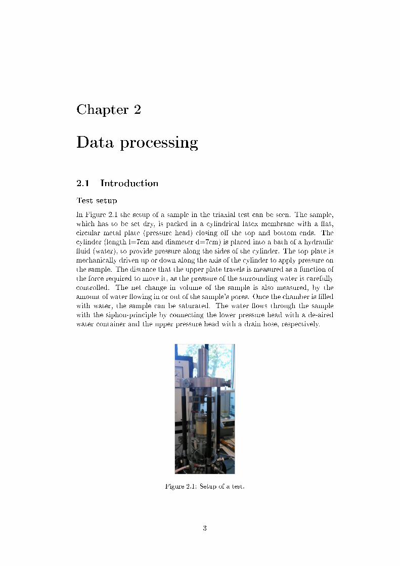
In Figure 2.1 the setup of a sample in the triaxial test can be seen. The sample,which has to be set dry, is packed in a cylindrical latex membrane with a �at,circular metal plate (pressure head) closing o� the top and bottom ends. Thecylinder (length l=7cm and diameter d=7cm) is placed into a bath of a hydraulic�uid (water), to provide pressure along the sides of the cylinder. The top plate ismechanically driven up or down along the axis of the cylinder to apply pressure onthe sample. The distance that the upper plate travels is measured as a function ofthe force required to move it, as the pressure of the surrounding water is carefullycontrolled. The net change in volume of the sample is also measured, by theamount of water �owing in or out of the sample's pores. Once the chamber is �lledwith water, the sample can be saturated. The water �ows through the samplewith the siphon-principle by connecting the lower pressure head with a de-airedwater container and the upper pressure head with a drain hose, respectively.
Figure 2.1: Setup of a test.
3
Measured parameters
The parameters measured in the triaxial test are the axial displacement ∆H, theheight of the sample using LVDT's, the change in volume ∆Wwater by the amountof water �owing in or out the sample, the chamber pressure σr and the axial loadapplied by the piston on the upper pressure head σa − σr.
Sand type
The sand type deployed in the triaxial tests is a Fontainebleau sand. Fontainebleausand is a well-sorted, clean sand with a particle size ranging from 0.063mm to0.25mm, and a uniformly index of U < 2. Further classi�cation parameters aregiven in Table 2.1 and they have been determined according to Dansk geotekniskforening (DGF)-Bulletin 15 (2001).
Relative grain density ds 2.655Densest deposition emin 0.549Loosest deposition emax 0.853
Table 2.1: Classi�cation parameters for sand
Experimental series
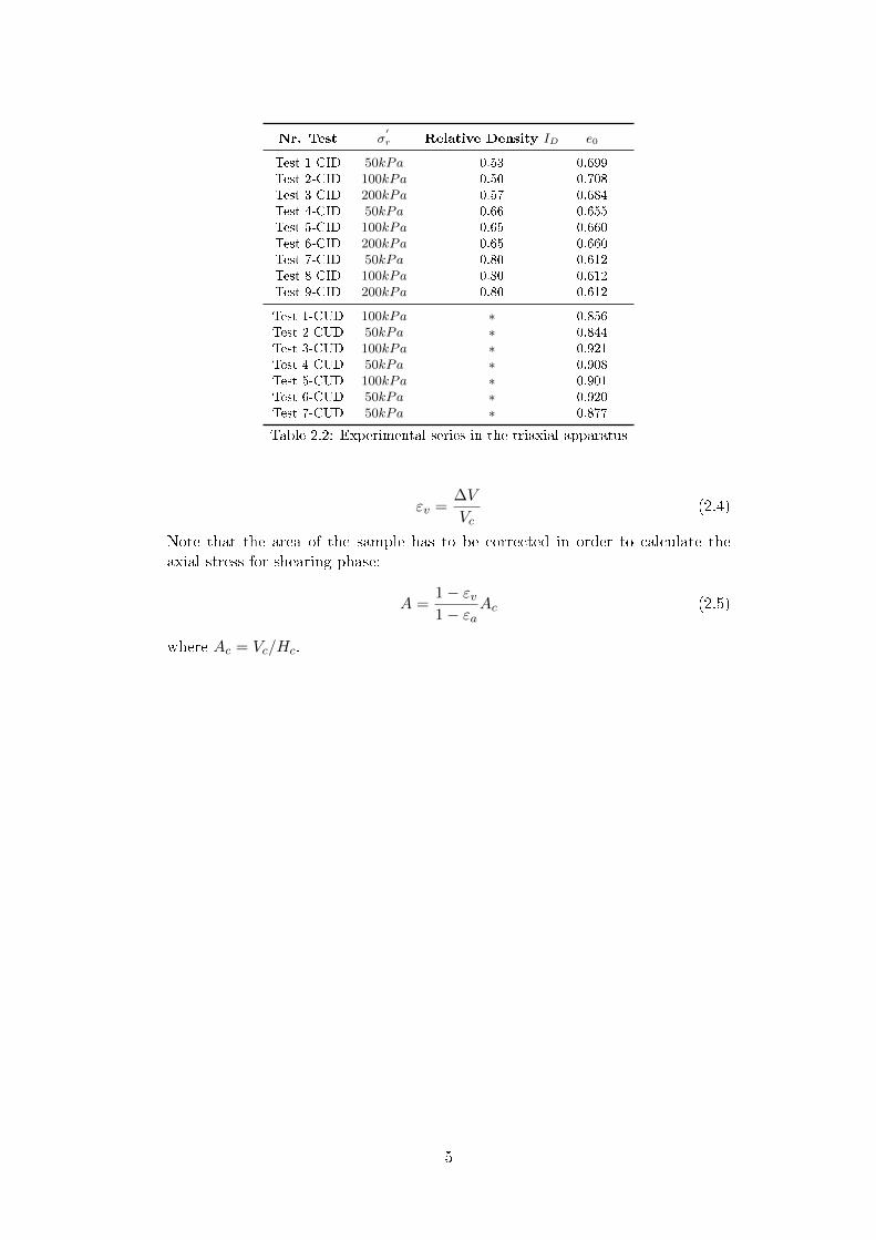
Samples at various relative densities ID were tested in drained and undrainedtriaxial compression conditions after having been isotropically consolidated (CID-CUD) to various cell pressures σ′r. The shear phase is done under both drainedand undrained conditions. The axial deformation rate is ε′a = 1%/ hour. At ap-proximately 50% of the expected peak deviatoric stress, qpeak, an unloading andreloading cycle was performed after which the sample was loaded in displacementcontrol to full failure (approximately 15% axial strain εa). The test series is sum-marized in Table 2.2. Note that the relative density for the test series performedin undrained conditions cannot be determined, since the samples are looser thanthe loosest deposition, see Table 2.2.
2.2 Measurement corrections
Calculation of axial and volumetric strains requires accurate estimation of theinitial height and area of the sample thus, corrections of the data have to beperformed. According to the speci�cations of ETCS-F1.97 several corrections onthe geometry of the samples have been applied for processing the data. The heightand volume of sample after consolidation are given as:
Hc = H0(1 − εa) (2.1)
Vc = V0 − ∆Vc (2.2)
where ∆Vc = ∆Wwater/%water. The axial and volumetric strain should be cal-culated, initializing the variations of height and volume at the beginning of theshearing phase. Thus, they are corrected according to:
εa =∆H
Hc(2.3)
4
Nr. Test σ′r Relative Density ID e0
Test 1-CID 50kPa 0.53 0.699
Test 2-CID 100kPa 0.50 0.708
Test 3-CID 200kPa 0.57 0.684
Test 4-CID 50kPa 0.66 0.655
Test 5-CID 100kPa 0.65 0.660
Test 6-CID 200kPa 0.65 0.660
Test 7-CID 50kPa 0.80 0.612
Test 8-CID 100kPa 0.80 0.612
Test 9-CID 200kPa 0.80 0.612
Test 1-CUD 100kPa ∗ 0.856
Test 2-CUD 50kPa ∗ 0.844
Test 3-CUD 100kPa ∗ 0.921
Test 4-CUD 50kPa ∗ 0.908
Test 5-CUD 100kPa ∗ 0.901
Test 6-CUD 50kPa ∗ 0.920
Test 7-CUD 50kPa ∗ 0.877
Table 2.2: Experimental series in the triaxial apparatus
εv =∆V
Vc(2.4)
Note that the area of the sample has to be corrected in order to calculate theaxial stress for shearing phase:
A =1 − εv1 − εa
Ac (2.5)
where Ac = Vc/Hc.
5

Chapter 3
Results
3.1 Consolidation phase
The bulk modulus K is a measure the compressibility of the sand. It is estimatedduring the consolidation phase as the slope of the axial stress p versus volumetricstrain εv plot. Therefore it can be calculated according to:
δp
δεv= K (3.1)
The bulk modulus for all drained triaxial tests is listed in Table 3.1.
Test K
Test 1-CID 27.6MPaTest 2-CID 38.0MPaTest 3-CID 43.7MPa
Test 4-CID 30.9MPaTest 5-CID 42.5MPaTest 6-CID 43.0MPa
Test 7-CID 38.5MPaTest 8-CID 43.9MPaTest 9-CID 55.3MPa
Table 3.1: Bulk modulus K for all drained triaxial tests.
When the relative density of the sand is increased the sample becomes lesscompressible and hence a higher bulk modulus is expected. Also, for higher valuesof the con�nement pressure it is expected that K will increase due to the increasein the radial pressure. The results seem to con�rm this trend. The lowest bulkmodulus was found for the Test 1, which has the lowest relative density and initialcon�ning pressure. The highest bulk modulus was recorded for Test 9, which hasthe highest cell pressure and relative density, as it is expected.
3.2 Elasticity parameters
The elastic sti�ness parameters of the soil are obtained from the shearing phaseof the test. Depending on the plot the gradient in this phase will give Young's
6
Modulus, E, the shear Modulus, G, and Poisson's ratio, υ. The shear modulus isgiven as the slope of the deviatoric stress, δq versus the shear strain δεq diagramdescribing the material's response to shear stress:
δq
δεq= 3G (3.2)
Young's Modulus describes the resistance of the sand when it is deformed elas-tically. It is given as the slope of the deviatoric stress δq versus the axial strainδεa:
δq
δεa= E (3.3)
Both E and G can be estimated theoretically from the initial shearing of thesample, Ei and Gi, when only elastic deformations occur. Hence Ei and Gi shouldbe equal respectively to E and G, if the measurements of the triaxial setup areaccurate in the low strains regime. The secant moduli E50 and Gsec are derivedas the slope of
δqmax,50
δεa= E50 (3.4)
δqmax,50
δεq= 3Gsec (3.5)
where qmax,50 is 50% of the expected maximum stress value. Poisson's ratio υ,can be evaluated by plotting the εa and εr, where εr is the radial strain. For theestimation of υ the unloading and reloading phase is deployed and Poisson's ratiois given as follows:
δεrδεa
= υ (3.6)
The expected values for the Poisson's ratio is in the order of [0.20; 0.30].
3.2.1 Unloading-reloading phase
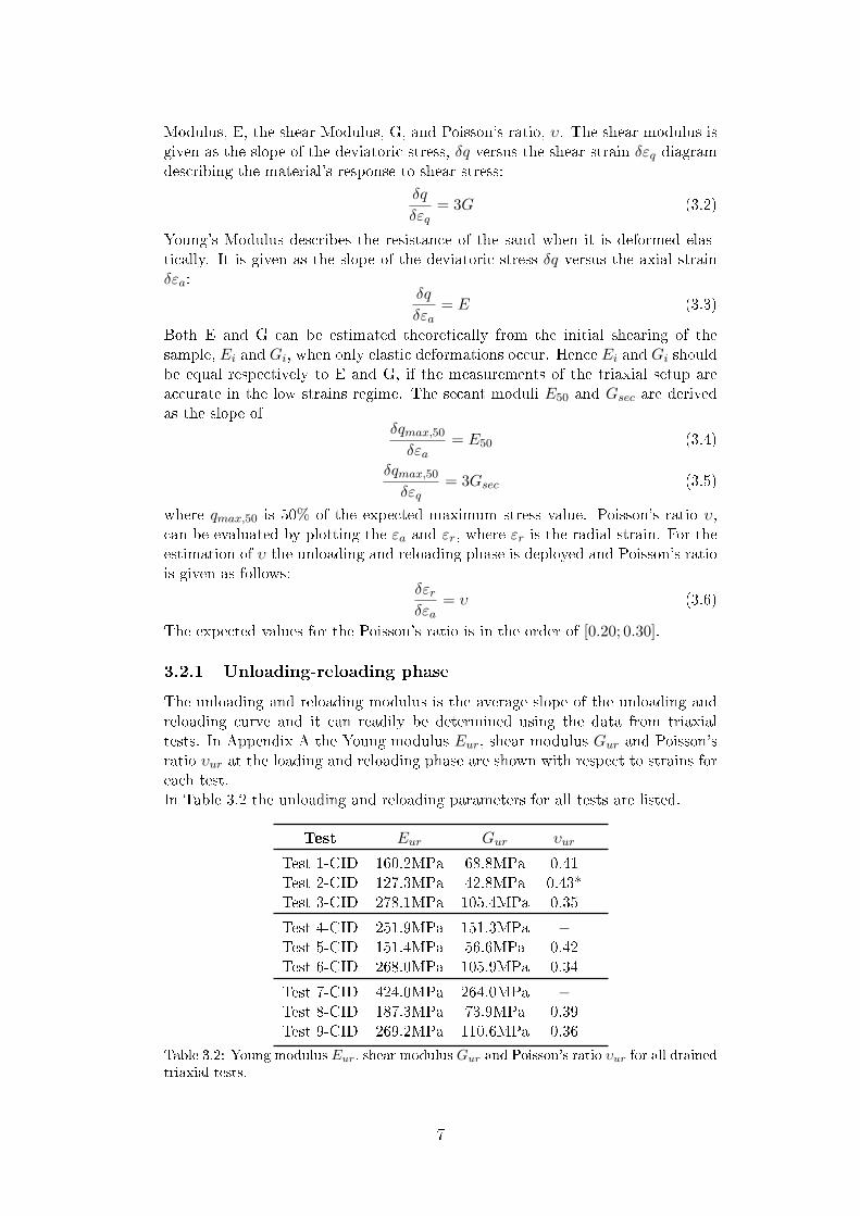
The unloading and reloading modulus is the average slope of the unloading andreloading curve and it can readily be determined using the data from triaxialtests. In Appendix A the Young modulus Eur, shear modulus Gur and Poisson'sratio υur at the loading and reloading phase are shown with respect to strains foreach test.In Table 3.2 the unloading and reloading parameters for all tests are listed.
Test Eur Gur υur
Test 1-CID 160.2MPa 68.8MPa 0.41Test 2-CID 127.3MPa 42.8MPa 0.43*Test 3-CID 278.1MPa 105.4MPa 0.35
Test 4-CID 251.9MPa 151.3MPa −Test 5-CID 151.4MPa 56.6MPa 0.42Test 6-CID 268.0MPa 105.9MPa 0.34
Test 7-CID 424.0MPa 264.0MPa −Test 8-CID 187.3MPa 73.9MPa 0.39Test 9-CID 269.2MPa 110.6MPa 0.36
Table 3.2: Young modulus Eur, shear modulus Gur and Poisson's ratio υur for all drainedtriaxial tests.
7
Duncan et al. (1970) showed that Eur and Gur increase with increases in thecon�ning pressure, but they are independent of the stress level. This pattern isrecorded for loose and dense sand samples, respectively Test 1,3, Test 4,6 andTest 8,9.In addition, it is noticed that the moduli tends to be higher if the particle areclosely packed (dense samples). This is evident by comparing the outcomes ofTest 1,4 and Test 2,5,8. Consequently, it is expected that the highest value of Eur
and Gur is reached in Test 9, where we have the highest initial con�ning pressureand relative density. However, Test 7 has showed the maximum value of Eur andGur.Poisson's ratio obtained from the unloading and reloading phase attains highervalues than those expected for drained sandy samples. In Test 3, Poisson's ratiocannot be estimated graphically, hence it is obtained according to:
G =E
2(1 + υ)(3.7)
A graphical estimation of Poisson's ratio in Test 4 is not feasible. Due to thehigh shear modulus value, the numerical calculations resulted in a negative valueand was not considered as a reliable result for Poisson's ratio, since that wouldbe physically impossible. Furthermore, in Test 7 the estimation of Poisson's ratiocannot be considered reliable, due to the positive slope of the trendline of theunloading/reloading line in εr and εa.No clear trend is seen for the Poisson's ratio in terms of con�nement pressureor relative density. It is observed a small decrease in Poisson's ratio for sampleswith the same relative density, when the con�ning pressure increases. In termsof relative density it would be expected to see an increase in Poisson's ratio withincreasing relative density; however the outcomes do not indicate this trend.
8

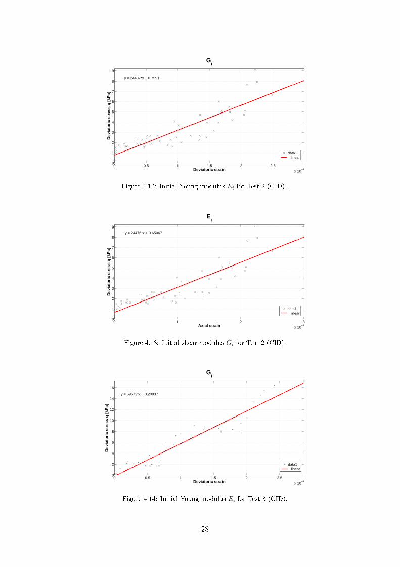
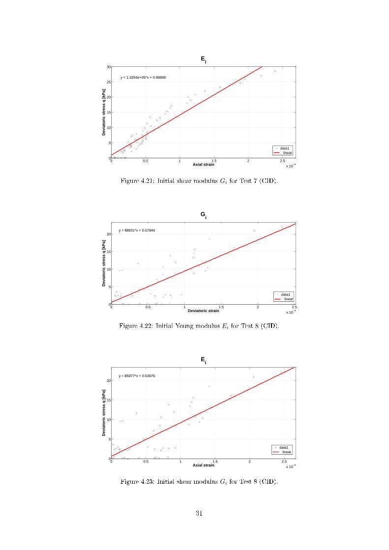
3.2.2 Initial moduli
The initial modulus is applicable only to very small deformations. Tatsuoka et al.(1997), Cuccovillo and Coop (1997) and Hoque and Tatsuoka (2004) showed thatthe deformation characteristics of sand samples are linear and elastic at strainsof less than approximately 0.001%. In addition, the small-strain measurementrequires relatively high accuracy. Therefore a signi�cant small strain interval εa =[0; 3e−4] has been considered for the estimation of the initial moduli. The initialYoung modulus Ei, shear modulus Gi and Poisson ratio υi are calculated andreported for each test in Appendix B. In Table 3.3 the initial elastic parametersfor all drained triaxial tests are listed.
Test Ei Gi υi
Test 1-CID 24.7MPa 8.13MPa 0.48Test 2-CID 24.4MPa 8.13MPa −Test 3-CID 69.9MPa 59.5MPa −Test 4-CID 45.1MPa 19.8MPa 0.20Test 5-CID 19.3MPa 3.9MPa −Test 6-CID 110.1MPa 30.6MPa 0.29
Test 7-CID 13.2MPa 5.1MPa 0.30Test 8-CID 85.8MPa 29.6MPa 0.44Test 9-CID 13.4MPa 9.0MPa 0.22
Table 3.3: Young modulus Ei, shear modulus Gi and Poisson's ratio υi for all drainedtriaxial tests.
Young's modulus Ei and shear modulus Gi are generally similar, see Test 1and 2. This might be explained by the fact that the volumetric strains are nearconstant in the low strains range.In addition, the value of Poisson's ratio is not feasible for Test 2,3 and 5, sincePoisson's ratio cannot overcome 0.5 and then, it is not presented in Table 3.3. Itcan be stated that the outcomes in the low strain range are considerably scat-tered; therefore they are not reliable.
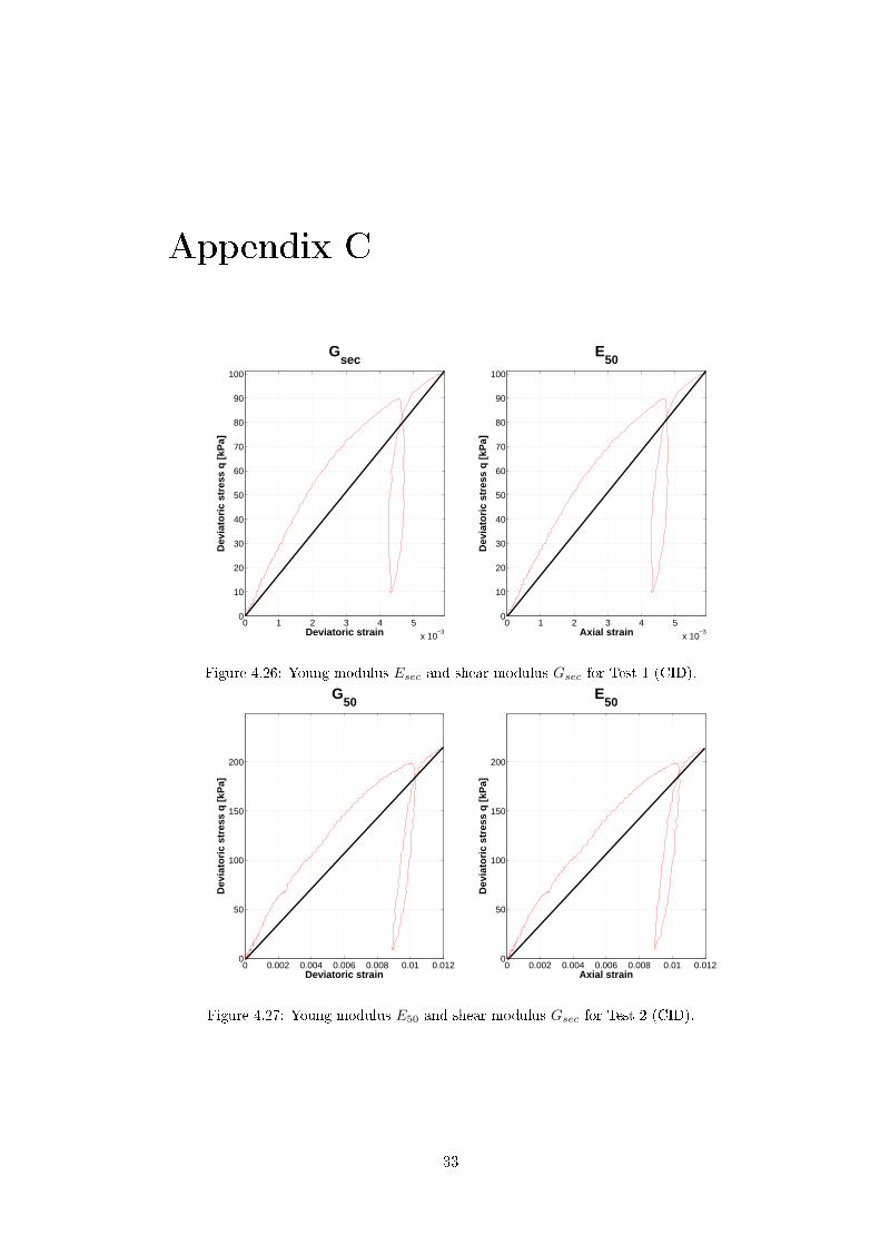
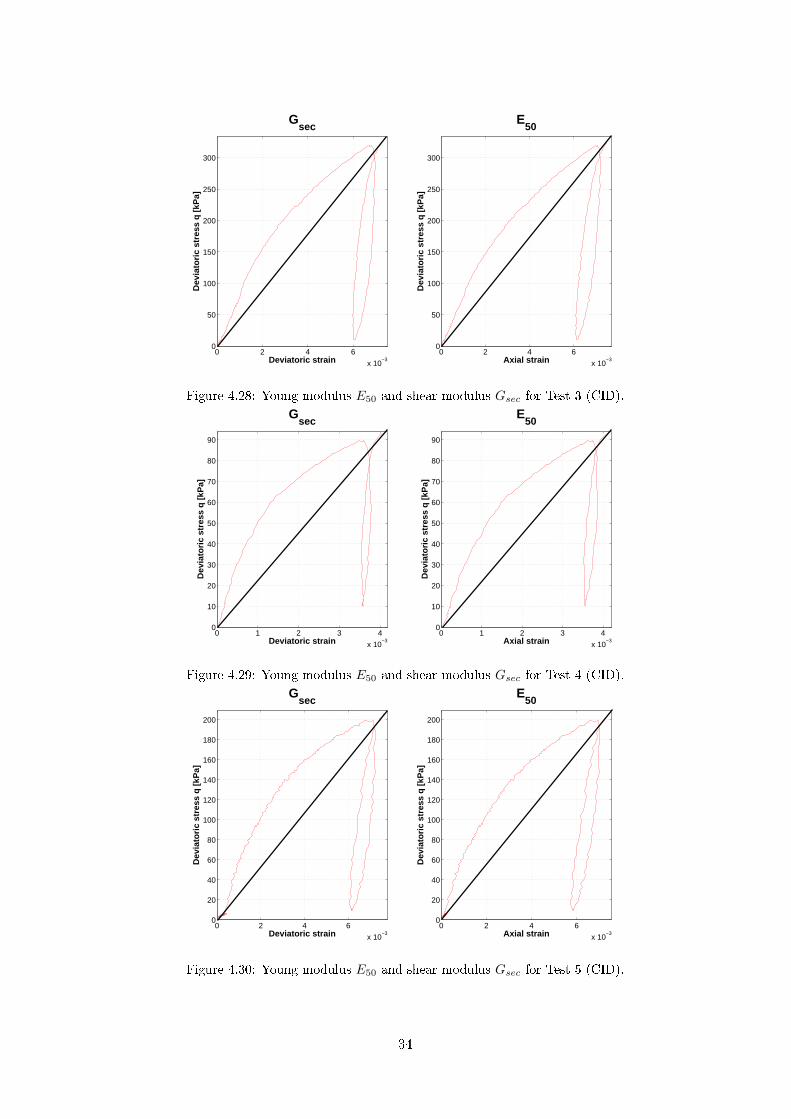
3.2.3 Secant moduli
The secant moduli are de�ned as the secant slope from the origin to a chosenpoint on the stress-strain curve. Note that the secant modulus does not respectthe de�nition of elastic modulus in the classical elasticity theory, due to the factthat elastic deformation and plastic deformation develop simultaneously. In Table3.4 the results of the secant moduli are listed for all drained triaxial tests. Itis expected that the secant moduli increase by increasing the initial con�ningpressure σ
′r. Results show this pattern. Regarding dense sands, Test 7 and 8 are
characterized by similar outcomes. The outcomes further indicate that relativedensity has a considerably in�uence in E50 and Gsec. Indeed, secant moduliincreases by increasing the relative density. The maximum value of E50 and Gsec
is attained in Test 6 and it is not in agreement with the prevision. Hence, it isexpected that the test with the highest con�ning pressure and relative densityprovides the maximum value of elastic moduli. Furthermore, it has been noticed
9

that 3Gsec and E50 are almost identical. This can be explained by the fact thein�uence of the volumetric strains is considerably small for the range of straininvestigated.
Test E50 Gsec
Test 1-CID 17.0MPa 5.7MPaTest 2-CID 22.6MPa 7.8PaTest 3-CID 43.2MPa 14.8MPa
Test 4-CID 22.3MPa 7.5MPaTest 5-CID 27.7MPa 8.9MPaTest 6-CID 86.3MPa 27.7MPa
Test 7-CID 32.9MPa 11.3MPaTest 8-CID 33.2MPa 11.5MPaTest 9-CID 60.4MPa 20.8MPa
Table 3.4: Young modulus Esec and shear modulus Gsec for all drained triaxial tests.
It is of interest to note that Young's modulus Eur can be calculated accordingto Marcher and Vermeer (2001) as follows:
Eur = 4E50 (3.8)
Equation 3.8 underestimates signi�cantly Young's modulus Eur particularly forloose and medium dense sand.
10

3.3 Estimation of strength parameters of CID tests
The experimental data included plots of deviatoric stress versus deviatoric strain,as well as volumetric strain versus deviatoric strain, for a range of di�erent con-�ning pressures and void ratios, see Figure 3.1, 3.2 and 3.3.
0 0.05 0.1 0.15 0.20
100
200
300
400
500
600
700
Axial strain
Dev
iato
ric
stre
ss q
[kP
a]
Test 1Test 2Test 3
0 0.05 0.1 0.15 0.2−0.1
−0.08
−0.06
−0.04
−0.02
0
0.02
Axial strain
Dev
iato
ric
stra
in
Test 1Test 2Test 3
Figure 3.1: Variation of deviatoric stress versus axial strain and volumetric strain versusaxial strain for Test 1, 2 and 3 (CID).
0 0.05 0.1 0.15 0.2 0.250
100
200
300
400
500
600
700
Axial strain
Dev
iato
ric
stre
ss q
[kP
a]
Test 4Test 5Test 6
0 0.05 0.1 0.15 0.2 0.25−0.12
−0.1
−0.08
−0.06
−0.04
−0.02
0
0.02
Axial strain
Dev
iato
ric
stra
in
Test 4Test 5Test 6
Figure 3.2: Variation of deviatoric stress versus axial strain and volumetric strain versusaxial strain for Test 4,5 and 6 (CID).
0 0.05 0.1 0.15 0.2 0.250
100
200
300
400
500
600
700
Axial strain
Dev
iato
ric
stre
ss q
[kP
a]
Test 7Test 8Test 9
0 0.05 0.1 0.15 0.2 0.25−0.14
−0.12
−0.1
−0.08
−0.06
−0.04
−0.02
0
0.02
Axial strain
Dev
iato
ric
stra
in
Test 7Test 8Test 9
Figure 3.3: Variation of deviatoric stress versus axial strain and volumetric strain versusaxial strain for Test 7,8 and 9 (CID).
The failure states in terms of p, q are used to determine the strength of thesoil. The yield surface of Mohr-Coloumb criterion is presented in Equation 3.9.
q = Mp′ + d (3.9)
The strength characteristics of the soil are then the angle of friction ϕ and thecohesion c. The friction angle describes how well a soil sample can withstand shearstress. During shearing, the friction angle can be found as the angle between thenormal force and the resultant force. While the cohesion c describes how a sampleresists against a shearing deformation caused by a shear force. For Id = 0.5 afriction angle between 30 ◦ and 35 ◦ is expected. For the sample of Id = 0.65the friction angle is expected to be higher and in the range of 35 ◦ and 40 ◦. For
11
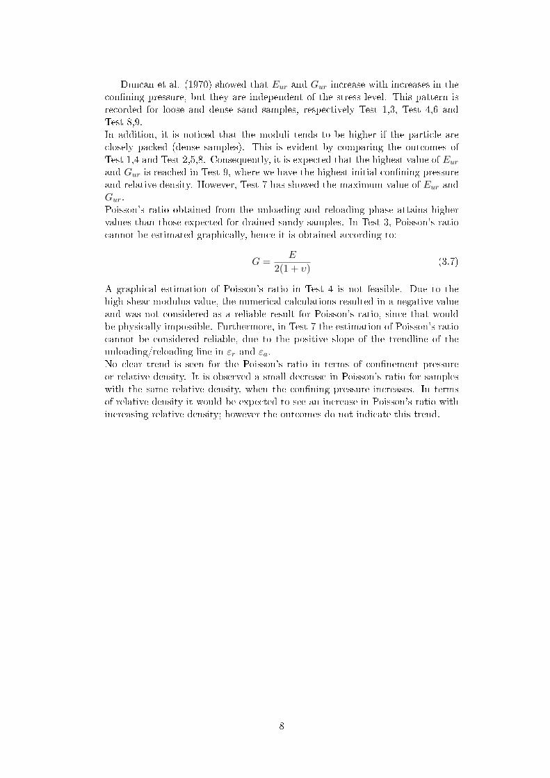
dense sand samples (Id > 0.80) an angle of friction in the interval of [40◦; 42◦] isusually considered. At failure the mobilized friction angle (ϕ) reaches to its �nalvalue.
M =(6 sinϕf )
(3 − sinϕf )(3.10)
The strength characteristics of this model can be obtained by plotting the fail-ure states in terms of (p,q) and �nding the best regression line to them. Therefore,the friction angle and the cohesion can be obtained as following:
ϕf = sin−1(
3M
6 +M
)(3.11)
c =d tan(ϕf )
M(3.12)
where d is the interecept of the failure line. No or very little cohesion in the orderof [0; 10]kPa is expected. In Table 3.5 the stresses (p,qpeak) and the strains (εv,εq)at the failure are reported.
Test qpeak p εq εv
Test 1-CID 197.3kPa 114.8kPa 7.12e-2 -3.46e-2Test 2-CID 310.8kPa 204.6kPa 1.23e-1 -3.76e-2Test 3-CID 649.7kPa 415.8kPa 8.75e-2 -3.50e-2
Test 4-CID 183.7kPa 113.7kPa 9.56e-2 -4.73e-2Test 5-CID 319.8kPa 205.2kPa 8.77e-2 -3.72e-2Test 6-CID 558.9kPa 387.6kPa 8.05e-2 -2.80e-2
Test 7-CID 210.2kPa 120.9kPa 9.34e-2 -5.64e-2Test 8-CID 358.8kPa 220.6kPa 8.36e-2 -4.27e-2Test 9-CID 698.9kPa 434.2kPa 7.56e-2 -3.70e-2
Table 3.5: Stress and strains at the failure for all drained triaxial tests.
The results in Table 3.5 show that the peak of deviatoric stress increasesfrom loose to dense sample by keeping the same initial con�ning pressure σ
′r,
as expected. Test 6 and Test 8 are characterized by an approximate value ofthe maximum deviatoric stress, since both triaxial tests did not reach 15% axialdeformation. Table 3.6 shows the slope of the critical state line M and the angleof friction ϕf for each drained triaxial test.
Set M ϕf
Test 1-CID 1.72 41.0Test 2-CID 1.52 37.3Test 3-CID 1.56 38.2Test 4-CID 1.61 39.8Test 5-CID 1.56 38.0Test 6-CID 1.50 37.0Test 7-CID 1.74 42.4Test 8-CID 1.62 39.8Test 9-CID 1.61 39.4
Table 3.6: Failure line parameters for all drained triaxial tests.
12

In Table 3.7 the value of M coe�cient (slope of the failure line), the angle offriction ϕf and the cohesion c at the failure are listed for all drained triaxialtests, gathered according to the same relative density. The failure line is shownin Figure 3.4, 3.5 and 3.6.
Set ID M ϕf c
Test 1,2 and 3 (CID) 0.50 1.50 36.9 6.5kPaTest 4,5 and 6 (CID) 0.66 1.50 36.9 9.5kPaTest 7,8 and 9 (CID) 0.80 1.59 39.2 9.1kPa
Table 3.7: Failure line parameters for all drained triaxial tests.
The friction angle is larger for dense sand which is consistent, since the frictionangle is greater if the sand is more compact. Indeed, the sand samples with highrelative density are generally characterized by high friction angle, see both Table3.6 and Table 3.7. It is evident that Test 1,2,3 and Test 4,5,6 are characterizedby the same angle friction. It is expected that Test 1,2,3 provide lower frictionangle, since they are loose sand samples.In addition, the larger friction angle leads to a steeper slope in the Cambridgediagram, which results in a smaller intersection value, hence a smaller e�ectivecohesion. This is not observed in the results achieved.
13

50 100 150 200 250 300 350 400 4500
100
200
300
400
500
600
700
Mean stress p [kPa]
Dev
iato
ric
stre
ss q
[kP
a]
Test 1
Test 2
Test 3
Failure line
Figure 3.4: Failure line for Test 1,2 and 3 (CID)
0 50 100 150 200 250 300 350 400 4500
100
200
300
400
500
600
700
Mean stress p [kPa]
Dev
iato
ric
stre
ss q
[kP
a]
Test 4
Test 5
Test 6
Failure line
Figure 3.5: Failure line for Test 4,5 and 6 (CID)
50 100 150 200 250 300 350 400 4500
100
200
300
400
500
600
700
Mean stress p [kPa]
Dev
iato
ric
stre
ss q
[kP
a]
Test 7
Test 8
Test 9
Failure line
Figure 3.6: Failure line for Test 7,8 and 9 (CID)
14

3.4 Estimation of strength parameters of CUD tests
In Figure 3.7−3.12 pore pressure and deviator stress versus axial strain are shownfor all the undrained tests. The pore pressure plotted with respect to axial strainshows a marked phase transformation from contraction (increase in pore pressure)to dilation (decrease in pore pressure) at about 2 − 2.5% axial strain.
0 0.05 0.1 0.15 0.2 0.25 0.3 0.350
50
100
150
200
250
300
350
Axial strain
Dev
iato
ric
stre
ss q
[kP
a]
Test 1
0 0.05 0.1 0.15 0.2 0.25 0.3 0.35−35
−30
−25
−20
−15
−10
−5
0
5
10
Axial strain
Po
re p
ress
ure
u [
kPa]
Figure 3.7: Variation of deviatoric stress versus axial strain and pore pressure versusaxial strain for Test 1 (CUD).
0 0.05 0.1 0.15 0.2 0.25 0.3 0.35 0.40
20
40
60
80
100
120
140
160
180
200
Axial strain
Dev
iato
ric
stre
ss q
[kP
a]
Test 2
0 0.05 0.1 0.15 0.2 0.25 0.3 0.35
−30
−25
−20
−15
−10
−5
0
5
10
Axial strain
Po
re p
ress
ure
u [
kPa]
Figure 3.8: Variation of deviatoric stress versus axial strain and pore pressure versusaxial strain for Test 2 (CUD).
0 0.05 0.1 0.15 0.2 0.25 0.3 0.35 0.40
50
100
150
200
250
300
Axial strain
Dev
iato
ric
stre
ss q
[kP
a]
Test 3
0 0.05 0.1 0.15 0.2 0.25 0.3 0.35 0.4−40
−30
−20
−10
0
10
20
30
Axial strain
Po
re p
ress
ure
u [
kPa]
Figure 3.9: Variation of deviatoric stress versus axial strain and pore pressure versusaxial strain for Test 3 (CUD).
15

0 0.05 0.1 0.15 0.2 0.25 0.3 0.35 0.40
20
40
60
80
100
120
140
160
180
200
Axial strain
Dev
iato
ric
stre
ss q
[kP
a]
Test 4
0 0.05 0.1 0.15 0.2 0.25 0.3 0.35 0.4
−40
−30
−20
−10
0
10
20
Axial strain
Po
re p
ress
ure
u [
kPa]
Figure 3.10: Variation of deviatoric stress versus axial strain and pore pressure versusaxial strain for Test 4 (CUD).
0 0.05 0.1 0.15 0.2 0.25 0.3 0.35 0.40
50
100
150
200
250
300
Axial strain
Dev
iato
ric
stre
ss q
[kP
a]
Test 5
0 0.05 0.1 0.15 0.2 0.25 0.3 0.35 0.4−40
−30
−20
−10
0
10
20
30
Axial strain
Po
re p
ress
ure
u [
kPa]
Figure 3.11: Variation of deviatoric stress versus axial strain and pore pressure versusaxial strain for Test 5 (CUD).
0 0.05 0.1 0.15 0.2 0.25 0.3 0.35 0.40
20
40
60
80
100
120
140
160
180
200
Axial strain
Dev
iato
ric
stre
ss q
[kP
a]
Test 6
0 0.05 0.1 0.15 0.2 0.25 0.3 0.35 0.4−40
−30
−20
−10
0
10
20
Axial strain
Po
re p
ress
ure
u [
kPa]
Figure 3.12: Variation of deviatoric stress versus axial strain and pore pressure versusaxial strain for Test 6 (CUD).
0 0.05 0.1 0.15 0.2 0.25 0.3 0.350
50
100
150
200
250
Axial strain
Dev
iato
ric
stre
ss q
[kP
a]
Test 7
0 0.05 0.1 0.15 0.2 0.25 0.3 0.35−50
−40
−30
−20
−10
0
10
20
30
Axial strain
Po
re p
ress
ure
u [
kPa]
Figure 3.13: Variation of deviatoric stress versus axial strain and pore pressure versusaxial strain for Test 7 (CUD).
16

While in Figure 3.14−3.17 the variation of the deviatoric stress q is illustratedwith respect to the mean stress p for each undrained triaxial test.
80 100 120 140 160 180 200 220 240 2600
50
100
150
200
250
300
350
Mean pressure p [kPa]
Dev
iato
ric
stre
ss q
[kP
a]
Test 1
40 60 80 100 120 140 1600
20
40
60
80
100
120
140
160
180
200
Mean pressure p [kPa]
Dev
iato
ric
stre
ss q
[kP
a]
Test 2
Figure 3.14: Variation of deviatoric stress versus mean stress for Test 1 and Test 2 (CUD).
80 100 120 140 160 180 200 220 2400
50
100
150
200
250
300
Mean pressure p [kPa]
Dev
iato
ric
stre
ss q
[kP
a]
Test 3
20 40 60 80 100 120 140 1600
20
40
60
80
100
120
140
160
180
200
Mean pressure p [kPa]
Dev
iato
ric
stre
ss q
[kP
a]
Test 4
Figure 3.15: Variation of deviatoric stress versus mean stress for Test 3 and Test 4 (CUD).
80 100 120 140 160 180 200 220 2400
50
100
150
200
250
300
Mean pressure p [kPa]
Dev
iato
ric
stre
ss q
[kP
a]
Test 5
20 40 60 80 100 120 140 1600
20
40
60
80
100
120
140
160
180
200
Mean pressure p [kPa]
Dev
iato
ric
stre
ss q
[kP
a]
Test 6
Figure 3.16: Variation of deviatoric stress versus mean stress for Test 5 and Test 6 (CUD).
20 40 60 80 100 120 140 160 1800
50
100
150
200
250
Mean pressure p [kPa]
Dev
iato
ric
stre
ss q
[kP
a]
Test 7
Figure 3.17: Variation of deviatoric stress versus mean stress for Test 7 (CUD).
17
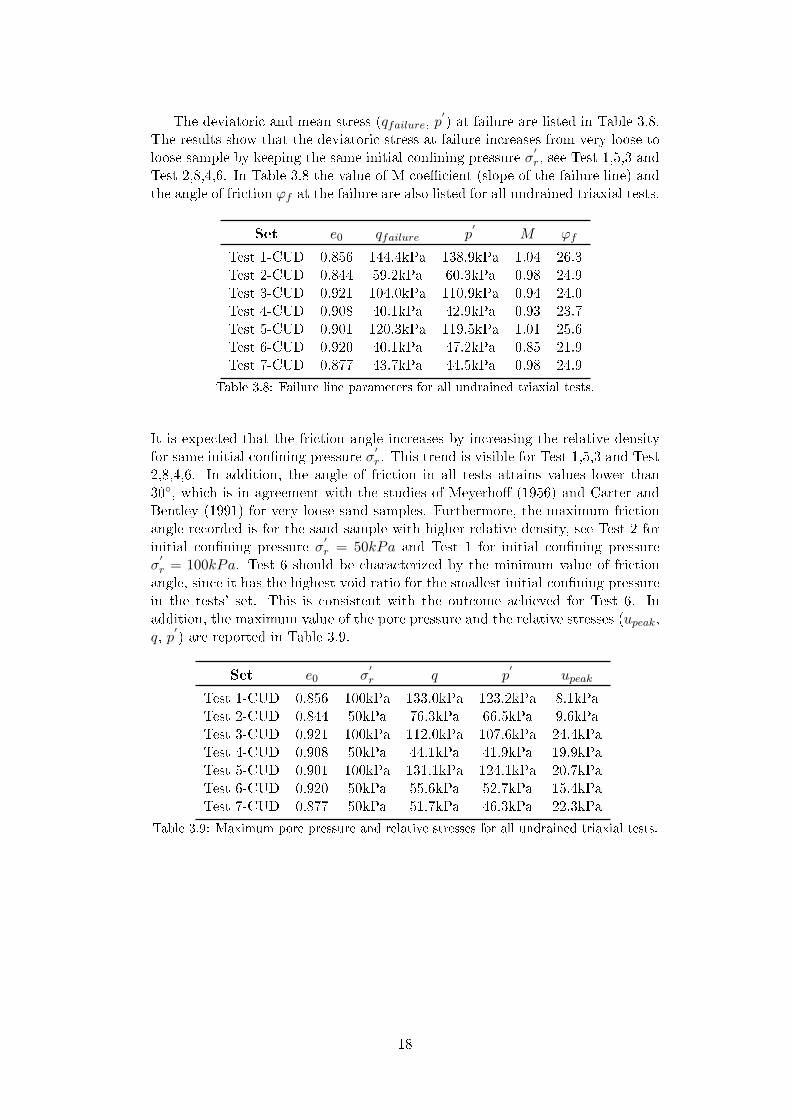
The deviatoric and mean stress (qfailure, p′) at failure are listed in Table 3.8.
The results show that the deviatoric stress at failure increases from very loose toloose sample by keeping the same initial con�ning pressure σ
′r, see Test 1,5,3 and
Test 2,8,4,6. In Table 3.8 the value of M coe�cient (slope of the failure line) andthe angle of friction ϕf at the failure are also listed for all undrained triaxial tests.
Set e0 qfailure p′
M ϕf
Test 1-CUD 0.856 144.4kPa 138.9kPa 1.04 26.3Test 2-CUD 0.844 59.2kPa 60.3kPa 0.98 24.9Test 3-CUD 0.921 104.0kPa 110.9kPa 0.94 24.0Test 4-CUD 0.908 40.1kPa 42.9kPa 0.93 23.7Test 5-CUD 0.901 120.3kPa 119.5kPa 1.01 25.6Test 6-CUD 0.920 40.1kPa 47.2kPa 0.85 21.9Test 7-CUD 0.877 43.7kPa 44.5kPa 0.98 24.9
Table 3.8: Failure line parameters for all undrained triaxial tests.
It is expected that the friction angle increases by increasing the relative densityfor same initial con�ning pressure σ
′r. This trend is visible for Test 1,5,3 and Test
2,8,4,6. In addition, the angle of friction in all tests attains values lower than30◦, which is in agreement with the studies of Meyerho� (1956) and Carter andBentley (1991) for very loose sand samples. Furthermore, the maximum frictionangle recorded is for the sand sample with higher relative density, see Test 2 forinitial con�ning pressure σ
′r = 50kPa and Test 1 for initial con�ning pressure
σ′r = 100kPa. Test 6 should be characterized by the minimum value of friction
angle, since it has the highest void ratio for the smallest initial con�ning pressurein the tests' set. This is consistent with the outcome achieved for Test 6. Inaddition, the maximum value of the pore pressure and the relative stresses (upeak,q, p
′) are reported in Table 3.9.
Set e0 σ′r q p
′upeak
Test 1-CUD 0.856 100kPa 133.0kPa 123.2kPa 8.1kPaTest 2-CUD 0.844 50kPa 76.3kPa 66.5kPa 9.6kPaTest 3-CUD 0.921 100kPa 112.0kPa 107.6kPa 24.4kPaTest 4-CUD 0.908 50kPa 44.1kPa 41.9kPa 19.9kPaTest 5-CUD 0.901 100kPa 131.1kPa 124.1kPa 20.7kPaTest 6-CUD 0.920 50kPa 55.6kPa 52.7kPa 15.4kPaTest 7-CUD 0.877 50kPa 51.7kPa 46.3kPa 22.3kPa
Table 3.9: Maximum pore pressure and relative stresses for all undrained triaxial tests.
18
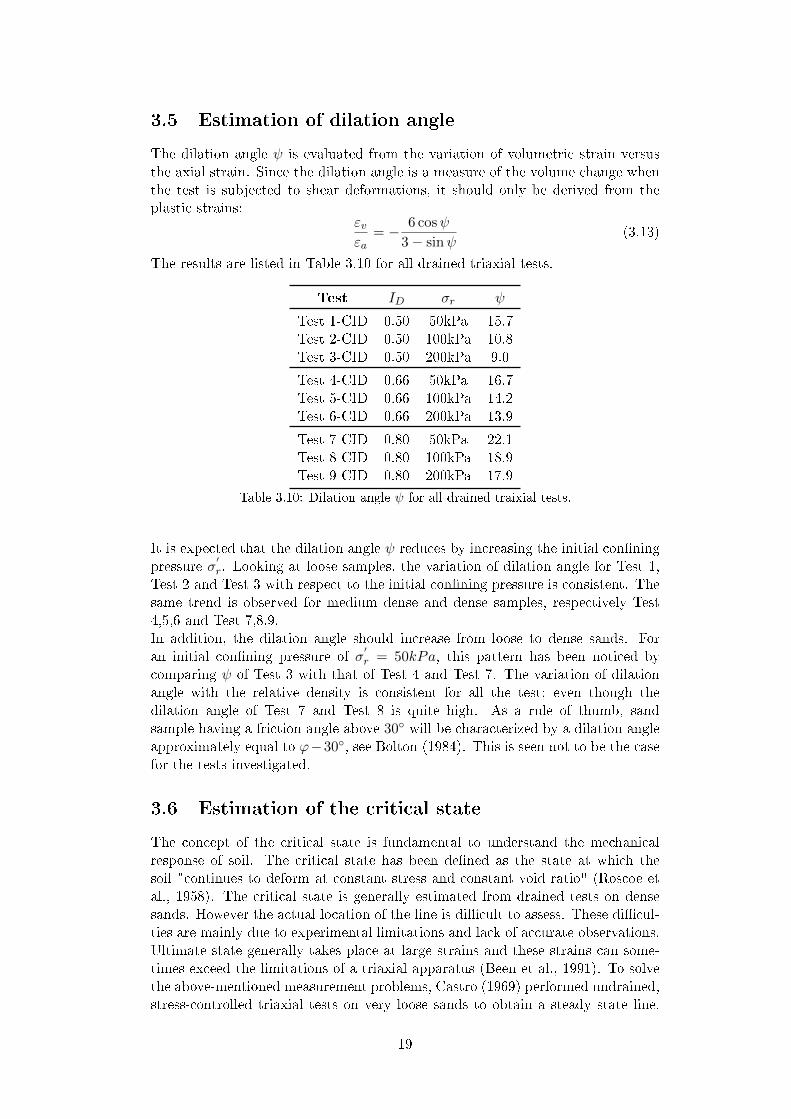
3.5 Estimation of dilation angle
The dilation angle ψ is evaluated from the variation of volumetric strain versusthe axial strain. Since the dilation angle is a measure of the volume change whenthe test is subjected to shear deformations, it should only be derived from theplastic strains:
εvεa
= − 6 cosψ
3 − sinψ(3.13)
The results are listed in Table 3.10 for all drained triaxial tests.
Test ID σr ψ
Test 1-CID 0.50 50kPa 15.7Test 2-CID 0.50 100kPa 10.8Test 3-CID 0.50 200kPa 9.0
Test 4-CID 0.66 50kPa 16.7Test 5-CID 0.66 100kPa 14.2Test 6-CID 0.66 200kPa 13.9
Test 7-CID 0.80 50kPa 22.1Test 8-CID 0.80 100kPa 18.9Test 9-CID 0.80 200kPa 17.9
Table 3.10: Dilation angle ψ for all drained traixial tests.
It is expected that the dilation angle ψ reduces by increasing the initial con�ningpressure σ
′r. Looking at loose samples, the variation of dilation angle for Test 1,
Test 2 and Test 3 with respect to the initial con�ning pressure is consistent. Thesame trend is observed for medium dense and dense samples, respectively Test4,5,6 and Test 7,8,9.In addition, the dilation angle should increase from loose to dense sands. Foran initial con�ning pressure of σ
′r = 50kPa, this pattern has been noticed by
comparing ψ of Test 3 with that of Test 4 and Test 7. The variation of dilationangle with the relative density is consistent for all the test; even though thedilation angle of Test 7 and Test 8 is quite high. As a rule of thumb, sandsample having a friction angle above 30◦ will be characterized by a dilation angleapproximately equal to ϕ−30◦, see Bolton (1984). This is seen not to be the casefor the tests investigated.
3.6 Estimation of the critical state
The concept of the critical state is fundamental to understand the mechanicalresponse of soil. The critical state has been de�ned as the state at which thesoil "continues to deform at constant stress and constant void ratio" (Roscoe etal., 1958). The critical state is generally estimated from drained tests on densesands. However the actual location of the line is di�cult to assess. These di�cul-ties are mainly due to experimental limitations and lack of accurate observations.Ultimate state generally takes place at large strains and these strains can some-times exceed the limitations of a triaxial apparatus (Been et al., 1991). To solvethe above-mentioned measurement problems, Castro (1969) performed undrained,stress-controlled triaxial tests on very loose sands to obtain a steady state line.
19

According to Poulos (1981), the steady state of deformation for any mass of parti-cles is that state in which the mass is continuously deforming at constant volume,constant normal e�ective stress, constant shear stress, and constant velocity. Beenet al. (1991) showed that the critical and steady state line are the same from apractical standpoint. Hence, the sample reaches the critical or steady state, whenit will experience large strains under monotonic loading. Furthermore, it was pro-posed a unique critical state line (CSL) for each sand in an e−logp′ plot which isindependent of type of loading, sample preparation method and initial density.In this study it is possible to detect the critical state in Test 5,7 and 9 (CID), seeFigure 3.1, 3.2 and 3.3, since shearing occurs with no volume change. In regardsto undrained conditions the occurrence of the critical state becomes visible in Test1,4,5,6 and 7(CUD) as shown in Figure 3.7, 3.10, 3.11, 3.12 and 3.13.Particularly, the critical state line can be obtained by plotting the results of tri-axial compression tests at the critical state in p−q space and �tting a best �t linethrough the data points as shown in Figure 3.18a. In addition, the void ratio atthe critical state ecr can be estimated by plotting undrained triaxial tests data ineln(p
′cr) space and �t them to a line having expression as shown in Figure 3.18b.
According to Been et al. (1991), this is a generally reasonable approximation forsub-angular or subrounded quartz sands in the stress range of 10−500kPa, whichis the case of the triaxial tests performed in this study.
Figure 3.18: Critical state line in q-p (a) and e−ln(p′cr) plane (b).
20

Chapter 4
Conclusions
The aim of this study was to present a series of triaxial tests carried out onFontainebleau sand in order to investigate the in�uence of the relative density onthe strength and deformation characteristics of this type of sand. In general thestrength parameters found seemed sensible and within the range of what wouldbe expected. For the elasticity parameters estimated in the unloading reload-ing phase no clear trend was seen for varying relative densities and con�nementpressure.
21

References
Been, K., Je�eries, M. G. and Hachey, J. 1991. Critical state of sands. Geotech-nique, 41(3), 365-381.
Bolton, M. D. 1984. The strength and dilatancy of sands. Cambridge UniversityEngineering Department.
Carter, M. and Bentley, S. 1991. Correlations of soil properties. Penetech PressPublishers, London.
Castro, G. 1969. Liquefaction of sands. ph. D. Thesis, Harvard Soil Mech.
Cuccovillo, T. and Coop, M. 1997. Yielding and prefailure deformation of struc-tured sands. Geotechnique, 47(3), 491-508.
Duncan, J.M. and Chang, C.Y. 1970. Nonlinear analysis of stress and strainin soils. Journal of Soil Mechanics, 96(5), 1629-1653.
Hoque, E. and Tatsuoka, F. 2004. E�ects of stress ratio on small strain sti�-ness during triaxial shearing. Geotechnique, 54(7), 429-439.
Marcher, T. and P. A. Vermeer. Macromodelling of softening in non-cohesivesoils. Continuous and discontinuous modelling of cohesive-frictional materials.Springer Berlin Heidelberg, 2001. 89-110.
Meyerhof, G. 1956. Penetration tests and bearing capacity of cohesionless soils.J Soils Mechanics and Foundation Division ASCE, 82(SM1).
Poulos, S. J. 1981. The steady state of deformation. Journal of Geotechnicaland Geoenvironmental Engineering, 107(ASCE 16241 Proceeding).
Roscoe, K. H., Scho�eld, A., and Wroth, C. P. 1958. On the yielding of soils.Geotechnique, 8(1), 22-53.
Tatsuoka, F., Sato, T., Park, C., Kim, Y.S., Mukabi, J.N: and Kohata, Y.1994a. Measurements of elastic properties of geomaterials in laboratory com-pression tests. Geotechnical Testing Journal, 17(1), 80-84.
22

Appendix A
4 4.5 5
x 10−3
0
50
100
150
Deviatoric strain
Dev
iato
ric
stre
ss q
[kP
a]
Gur
4 4.5 5
x 10−3
0
50
100
150
Axial strain
Dev
iato
ric
stre
ss q
[kP
a]
Eur
4 4.5 5
x 10−3
2
2.1
2.2
2.3
2.4
2.5
2.6
2.7
2.8
2.9
3x 10
−3
Axial strain
Rad
ial s
trai
n
vur
Figure 4.1: Young modulus Eur, shear modulus Gur and Poisson's ratio υur at unloadingand reloading phase for test 1 (CID).
8 9 10 11
x 10−3
0
50
100
150
200
Deviatoric strain
Dev
iato
ric
stre
ss q
[kP
a]
Gur
8 9 10 11
x 10−3
0
50
100
150
200
Axial strain
Dev
iato
ric
stre
ss q
[kP
a]
Eur
8 9 10 11
x 10−3
−6
−5
−4
−3
−2
−1
x 10−3
Axial strain
Rad
ial s
trai
n
vur
Figure 4.2: Young modulus Eur, shear modulus Gur and Poisson's ratio υur at unloadingand reloading phase for test 2 (CID).
23
6 7 8
x 10−3
0
50
100
150
200
250
300
350
400
450
500
Deviatoric strain
Dev
iato
ric
stre
ss q
[kP
a]
Gur
6 6.5 7 7.5 8
x 10−3
0
50
100
150
200
250
300
350
400
450
500
Axial strain
Dev
iato
ric
stre
ss q
[kP
a]
Eur
4 5 6 7 8
x 10−3
−4
−3
−2x 10
−3
Axial strain
Rad
ial s
trai
n
vur
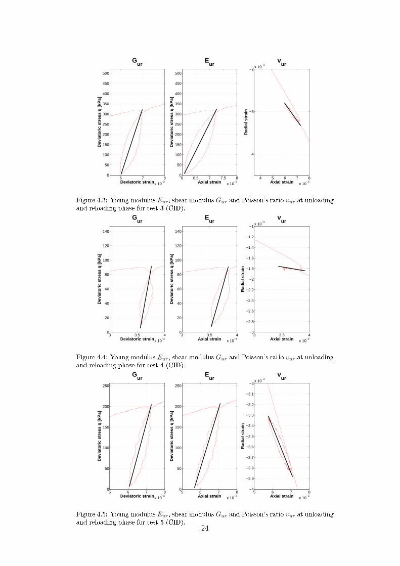
Figure 4.3: Young modulus Eur, shear modulus Gur and Poisson's ratio υur at unloadingand reloading phase for test 3 (CID).
3 3.5 4
x 10−3
0
20
40
60
80
100
120
140
Deviatoric strain
Dev
iato
ric
stre
ss q
[kP
a]
Gur
3 3.5 4
x 10−3
0
20
40
60
80
100
120
140
Axial strain
Dev
iato
ric
stre
ss q
[kP
a]
Eur
3 3.5 4
x 10−3
−3
−2.8
−2.6
−2.4
−2.2
−2
−1.8
−1.6
−1.4
−1.2
−1x 10
−3
Axial strain
Rad
ial s
trai
n
vur
Figure 4.4: Young modulus Eur, shear modulus Gur and Poisson's ratio υur at unloadingand reloading phase for test 4 (CID).
5 6 7 8
x 10−3
0
50
100
150
200
250
Deviatoric strain
Dev
iato
ric
stre
ss q
[kP
a]
Gur
5 6 7 8
x 10−3
0
50
100
150
200
250
Axial strain
Dev
iato
ric
stre
ss q
[kP
a]
Eur
5 6 7 8
x 10−3
−4
−3.9
−3.8
−3.7
−3.6
−3.5
−3.4
−3.3
−3.2
−3.1
−3x 10
−3
Axial strain
Rad
ial s
trai
n
vur
Figure 4.5: Young modulus Eur, shear modulus Gur and Poisson's ratio υur at unloadingand reloading phase for test 5 (CID).
24

3 4 5
x 10−3
−50
0
50
100
150
200
250
300
350
400
Deviatoric strain
Dev
iato
ric
stre
ss q
[kP
a]
Gur
2 3 4
x 10−3
−50
0
50
100
150
200
250
300
350
400
Axial strainD
evia
tori
c st
ress
q [
kPa]
Eur
2 3 4
x 10−3
−4
−3.5
−3
−2.5
−2
−1.5
−1
−0.5
0
x 10−3
Axial strain
Rad
ial s
trai
n
vur
Figure 4.6: Young modulus Eur, shear modulus Gur and Poisson's ratio υur at unloadingand reloading phase for test 6 (CID).
2 2.5 3
x 10−3
0
20
40
60
80
100
120
Deviatoric strain
Dev
iato
ric
stre
ss q
[kP
a]
Gur
2 2.5 3
x 10−3
0
20
40
60
80
100
120
Axial strain
Dev
iato
ric
stre
ss q
[kP
a]
Eur
2 2.2 2.4 2.6
x 10−3
−1.4
−1.3
−1.2
−1.1
−1
−0.9
−0.8
−0.7
−0.6
x 10−3
Axial strain
Rad
ial s
trai
n
vur
Figure 4.7: Young modulus Eur, shear modulus Gur and Poisson's ratio υur at unloadingand reloading phase for test 7 (CID).
4 4.5 5 5.5 6
x 10−3
0
20
40
60
80
100
120
140
160
180
200
Deviatoric strain
Dev
iato
ric
stre
ss q
[kP
a]
Gur
4 4.5 5 5.5 6
x 10−3
0
20
40
60
80
100
120
140
160
180
200
Axial strain
Dev
iato
ric
stre
ss q
[kP
a]
Eur
4 4.5 5 5.5 6
x 10−3
−3.5
−3
−2.5
−2x 10
−3
Axial strain
Rad
ial s
trai
n
vur
Figure 4.8: Young modulus Eur, shear modulus Gur and Poisson's ratio υur at unloadingand reloading phase for test 8 (CID).
25

4 5 6 7
x 10−3
0
50
100
150
200
250
300
350
400
Deviatoric strain
Dev
iato
ric
stre
ss q
[kP
a]
Gur
4 5 6 7
x 10−3
0
50
100
150
200
250
300
350
400
Axial strain
Dev
iato
ric
stre
ss q
[kP
a]
Eur
4 5 6 7
x 10−3
−3.5
−3
−2.5
−2x 10
−3
Axial strain
Rad
ial s
trai
n
vur
Figure 4.9: Young modulus Eur, shear modulus Gur and Poisson's ratio υur at unloadingand reloading phase for test 9-CID.
26
Appendix B
0 0.5 1 1.5 2 2.5
x 10−4
0
1
2
3
4
5
6
Deviatoric strain
Dev
iato
ric
stre
ss q
[kP
a]
Gi
y = 24714*x − 0.028648
data1 linear
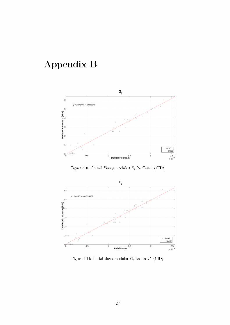
Figure 4.10: Initial Young modulus Ei for Test 1 (CID).
0 0.5 1 1.5 2 2.5
x 10−4
0
1
2
3
4
5
6
Axial strain
Dev
iato
ric
stre
ss q
[kP
a]
Ei
y = 24436*x + 0.055003
data1 linear
Figure 4.11: Initial shear modulus Gi for Test 1 (CID).
27
0 0.5 1 1.5 2 2.5
x 10−4
0
1
2
3
4
5
6
7
8
9
Deviatoric strain
Dev
iato
ric
stre
ss q
[kP
a]
Gi
y = 24437*x + 0.7591
data1 linear
Figure 4.12: Initial Young modulus Ei for Test 2 (CID)..
0 1 2 3
x 10−4
0
1
2
3
4
5
6
7
8
9
Axial strain
Dev
iato
ric
stre
ss q
[kP
a]
Ei
y = 24476*x + 0.65067
data1 linear
Figure 4.13: Initial shear modulus Gi for Test 2 (CID).
0 0.5 1 1.5 2 2.5
x 10−4
0
2
4
6
8
10
12
14
16
Deviatoric strain
Dev
iato
ric
stre
ss q
[kP
a]
Gi
y = 59572*x − 0.20837
data1 linear
Figure 4.14: Initial Young modulus Ei for Test 3 (CID).
28

0 0.5 1 1.5 2 2.5
x 10−4
0
2
4
6
8
10
12
14
16
Axial strain
Dev
iato
ric
stre
ss q
[kP
a]
Ei
y = 69922*x + 0.19432
data1 linear
Figure 4.15: Initial shear modulus Gi for Test 3 (CID).
0 1 2
x 10−4
0
2
4
6
8
10
12
Deviatoric strain
Dev
iato
ric
stre
ss q
[kP
a]
Gi
y = 57460*x − 0.40175
data1 linear
Figure 4.16: Initial Young modulus Ei for Test 4 (CID).
0 0.5 1 1.5 2 2.5
x 10−4
0
2
4
6
8
10
12
Axial strain
Dev
iato
ric
stre
ss q
[kP
a]
Ei
y = 45103*x − 0.21972
data1 linear
Figure 4.17: Initial shear modulus Gi for Test 4 (CID).
29

0 0.5 1 1.5 2 2.5 3 3.5 4 4.5
x 10−4
0
2
4
6
8
10
12
14
Deviatoric strain
Dev
iato
ric
stre
ss q
[kP
a]
Gi
y = 11653*x + 1.998
data1 linear
Figure 4.18: Initial Young modulus Ei for Test 5 (CID).
0 0.5 1 1.5 2 2.5
x 10−4
0
2
4
6
8
10
12
14
Axial strain
Dev
iato
ric
stre
ss q
[kP
a]
Ei
y = 19362*x + 2.1672
data1 linear
Figure 4.19: Initial shear modulus Gi for Test 5 (CID).
0 1 2
x 10−4
0
5
10
15
20
25
30
Deviatoric strain
Dev
iato
ric
stre
ss q
[kP
a]
Gi
y = 1.5323e+05*x − 0.087821
data1 linear
Figure 4.20: Initial Young modulus Ei for Test 7 (CID).
30
0 0.5 1 1.5 2 2.5
x 10−4
0
5
10
15
20
25
30
Axial strain
Dev
iato
ric
stre
ss q
[kP
a]
Ei
y = 1.3204e+05*x + 0.96896
data1 linear
Figure 4.21: Initial shear modulus Gi for Test 7 (CID).
0 0.5 1 1.5 2 2.5
x 10−4
0
5
10
15
20
Deviatoric strain
Dev
iato
ric
stre
ss q
[kP
a]
Gi
y = 88831*x + 0.57846
data1 linear
Figure 4.22: Initial Young modulus Ei for Test 8 (CID).
0 0.5 1 1.5 2 2.5
x 10−4
0
5
10
15
20
Axial strain
Dev
iato
ric
stre
ss q
[kP
a]
Ei
y = 85877*x + 0.63976
data1 linear
Figure 4.23: Initial shear modulus Gi for Test 8 (CID).
31

0 0.2 0.4 0.6 0.8 1 1.2
x 10−4
0
0.5
1
1.5
2
2.5
3
3.5
Deviatoric strain
Dev
iato
ric
stre
ss q
[kP
a]
Gi
y = 27092*x − 0.019529
data1 linear
Figure 4.24: Initial Young modulus Ei for Test 9 (CID).
0 0.5 1 1.5 2 2.5
x 10−4
0
0.5
1
1.5
2
2.5
3
3.5
Axial strain
Dev
iato
ric
stre
ss q
[kP
a]
Ei
y = 13410*x − 0.80613
data1 linear
Figure 4.25: Initial shear modulus Gi for Test 9 (CID).
32
Appendix C
0 1 2 3 4 5
x 10−3
0
10
20
30
40
50
60
70
80
90
100
Deviatoric strain
Dev
iato
ric
stre
ss q
[kP
a]
Gsec
0 1 2 3 4 5
x 10−3
0
10
20
30
40
50
60
70
80
90
100
Axial strain
Dev
iato
ric
stre
ss q
[kP
a]
E50
Figure 4.26: Young modulus Esec and shear modulus Gsec for Test 1 (CID).
0 0.002 0.004 0.006 0.008 0.01 0.0120
50
100
150
200
Deviatoric strain
Dev
iato
ric
stre
ss q
[kP
a]
G50
0 0.002 0.004 0.006 0.008 0.01 0.0120
50
100
150
200
Axial strain
Dev
iato
ric
stre
ss q
[kP
a]
E50
Figure 4.27: Young modulus E50 and shear modulus Gsec for Test 2 (CID).
33
0 2 4 6
x 10−3
0
50
100
150
200
250
300
Deviatoric strain
Dev
iato
ric
stre
ss q
[kP
a]
Gsec
0 2 4 6
x 10−3
0
50
100
150
200
250
300
Axial strain
Dev
iato
ric
stre
ss q
[kP
a]
E50
Figure 4.28: Young modulus E50 and shear modulus Gsec for Test 3 (CID).
0 1 2 3 4
x 10−3
0
10
20
30
40
50
60
70
80
90
Deviatoric strain
Dev
iato
ric
stre
ss q
[kP
a]
Gsec
0 1 2 3 4
x 10−3
0
10
20
30
40
50
60
70
80
90
Axial strain
Dev
iato
ric
stre
ss q
[kP
a]E
50
Figure 4.29: Young modulus E50 and shear modulus Gsec for Test 4 (CID).
0 2 4 6
x 10−3
0
20
40
60
80
100
120
140
160
180
200
Deviatoric strain
Dev
iato
ric
stre
ss q
[kP
a]
Gsec
0 2 4 6
x 10−3
0
20
40
60
80
100
120
140
160
180
200
Axial strain
Dev
iato
ric
stre
ss q
[kP
a]
E50
Figure 4.30: Young modulus E50 and shear modulus Gsec for Test 5 (CID).
34
0 1 2 3 4 5 6
x 10−3
0
50
100
150
200
250
300
350
400
Deviatoric strain
Dev
iato
ric
stre
ss q
[kP
a]
Gsec
0 1 2 3 4 5 6
x 10−3
0
50
100
150
200
250
300
350
400
Axial strain
Dev
iato
ric
stre
ss q
[kP
a]
E50
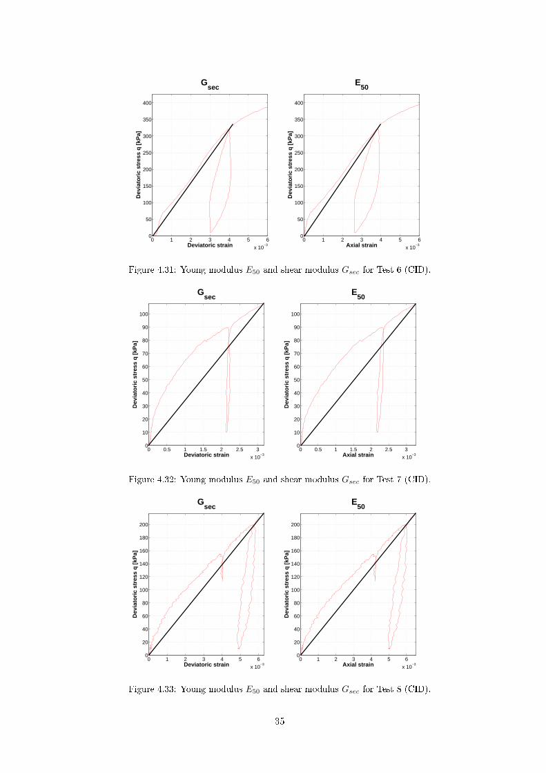
Figure 4.31: Young modulus E50 and shear modulus Gsec for Test 6 (CID).
0 0.5 1 1.5 2 2.5 3
x 10−3
0
10
20
30
40
50
60
70
80
90
100
Deviatoric strain
Dev
iato
ric
stre
ss q
[kP
a]
Gsec
0 0.5 1 1.5 2 2.5 3
x 10−3
0
10
20
30
40
50
60
70
80
90
100
Axial strain
Dev
iato
ric
stre
ss q
[kP
a]E
50
Figure 4.32: Young modulus E50 and shear modulus Gsec for Test 7 (CID).
0 1 2 3 4 5 6
x 10−3
0
20
40
60
80
100
120
140
160
180
200
Deviatoric strain
Dev
iato
ric
stre
ss q
[kP
a]
Gsec
0 1 2 3 4 5 6
x 10−3
0
20
40
60
80
100
120
140
160
180
200
Axial strain
Dev
iato
ric
stre
ss q
[kP
a]
E50
Figure 4.33: Young modulus E50 and shear modulus Gsec for Test 8 (CID).
35

0 2 4 6
x 10−3
0
50
100
150
200
250
300
350
400
Deviatoric strain
Dev
iato
ric
stre
ss q
[kP
a]
Gsec
0 1 2 3 4 5 6
x 10−3
0
50
100
150
200
250
300
350
400
Axial strain
Dev
iato
ric
stre
ss q
[kP
a]
E50
Figure 4.34: Young modulus E50 and shear modulus Gsec for Test 9 (CID).
36
Appendix D
0.02 0.04 0.06 0.08 0.1 0.12 0.14 0.16
−0.1
−0.09
−0.08
−0.07
−0.06
−0.05
−0.04
−0.03
−0.02
−0.01
0
Axial strain
Vo
lum
etri
c st
rain
Dilation angle
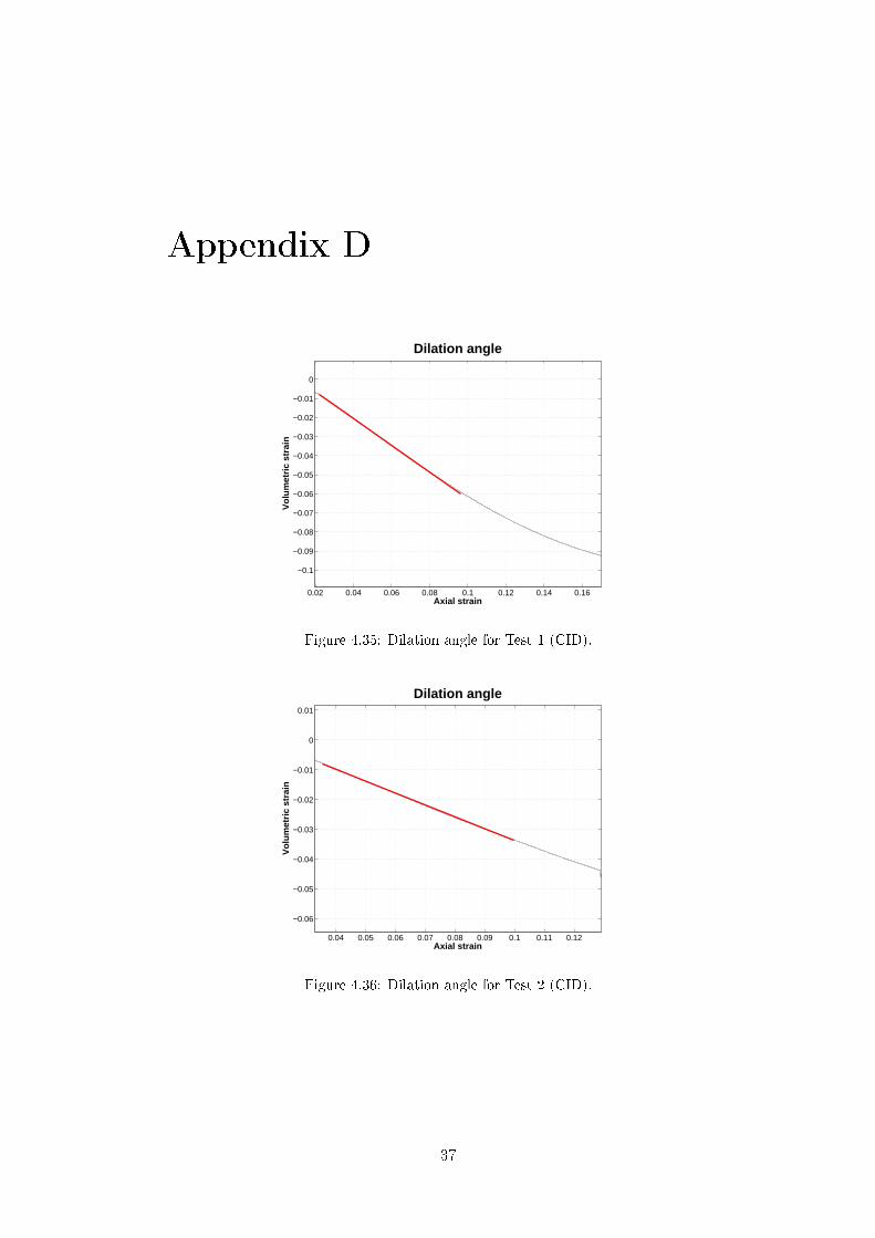
Figure 4.35: Dilation angle for Test 1 (CID).
0.04 0.05 0.06 0.07 0.08 0.09 0.1 0.11 0.12
−0.06
−0.05
−0.04
−0.03
−0.02
−0.01
0
0.01
Axial strain
Vo
lum
etri
c st
rain
Dilation angle
Figure 4.36: Dilation angle for Test 2 (CID).
37

0.02 0.04 0.06 0.08 0.1 0.12 0.14 0.16 0.18
−0.1
−0.08
−0.06
−0.04
−0.02
0
0.02
Axial strain
Vo
lum
etri
c st
rain
Dilation angle
Figure 4.37: Dilation angle for Test 3 (CID).
0.04 0.06 0.08 0.1 0.12 0.14 0.16 0.18 0.2 0.22 0.24
−0.14
−0.12
−0.1
−0.08
−0.06
−0.04
−0.02
0
0.02
Axial strain
Vo
lum
etri
c st
rain
Dilation angle
Figure 4.38: Dilation angle for Test 4 (CID).
0.02 0.04 0.06 0.08 0.1 0.12 0.14 0.16 0.18 0.2 0.22
−0.12
−0.1
−0.08
−0.06
−0.04
−0.02
0
0.02
Deviatoric strain
Axi
al s
trai
n
Dilation angle
Figure 4.39: Dilation angle for Test 5 (CID).
38

0.01 0.02 0.03 0.04 0.05 0.06 0.07 0.08
−0.05
−0.04
−0.03
−0.02
−0.01
0
0.01
Axial strain
Vo
lum
etri
c st
rain
Dilation angle
Figure 4.40: Dilation angle for Test 6 (CID).
0.04 0.06 0.08 0.1 0.12 0.14 0.16 0.18 0.2 0.22−0.15
−0.1
−0.05
0
Axial strain
Vo
lum
etri
c st
rain
Dilation angle
Figure 4.41: Dilation angle for Test 7 (CID).
0.02 0.03 0.04 0.05 0.06 0.07 0.08 0.09 0.1−0.07
−0.06
−0.05
−0.04
−0.03
−0.02
−0.01
Axial strain
Vo
lum
etri
c st
rain
Dilation angle
Figure 4.42: Dilation angle for Test 8 (CID).
39
0.02 0.04 0.06 0.08 0.1 0.12 0.14 0.16 0.18 0.2 0.22
−0.14
−0.12
−0.1
−0.08
−0.06
−0.04
−0.02
0
0.02
Vo
lum
etri
c st
rain
Axial strain
Dilation angle
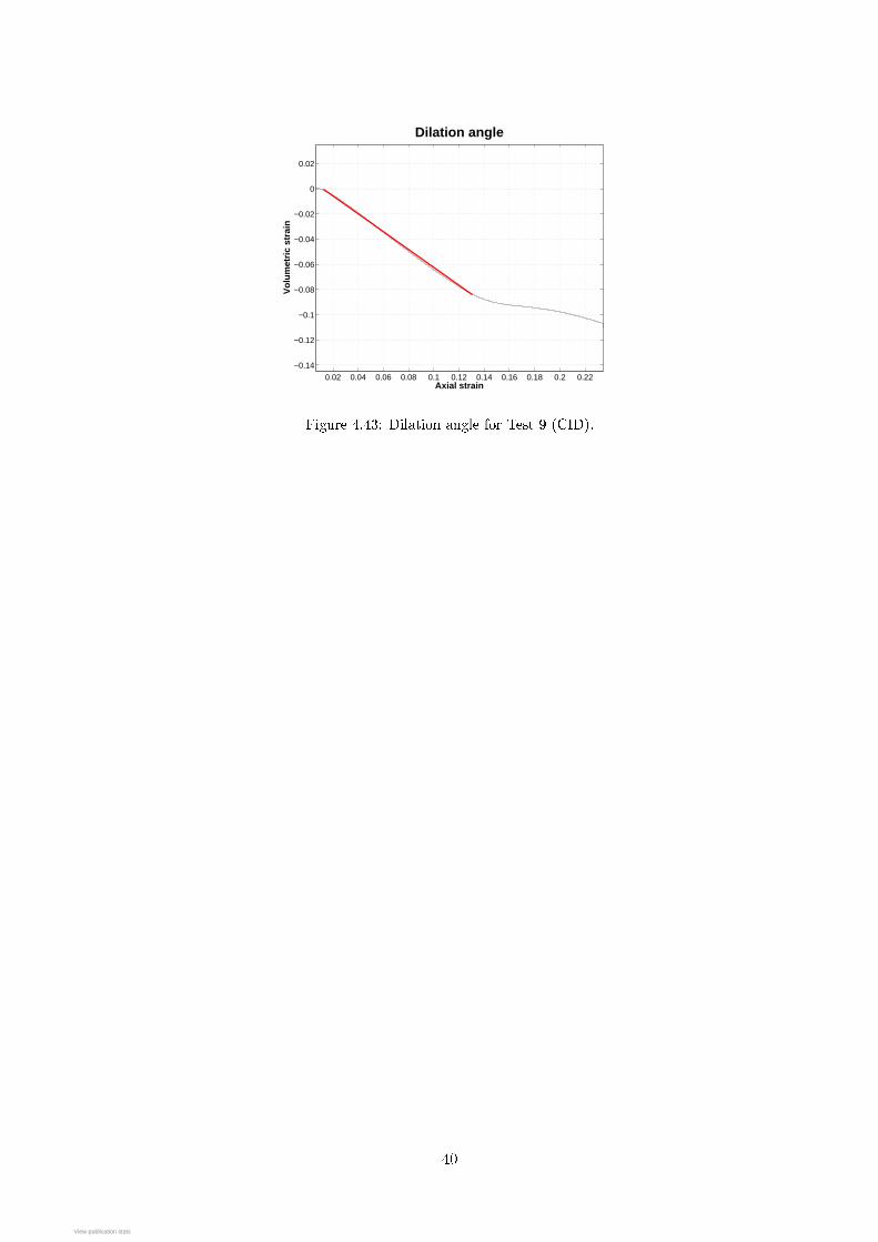
Figure 4.43: Dilation angle for Test 9 (CID).
40
View publication statsView publication stats