tridiagonal toeplitz matrices: properties and novel ...reichel/publications/toep3.pdf ·...

Tridiagonal Toeplitz Matrices: Properties and Novel Applications

Silvia Noschese1 Lionello Pasquini2 and Lothar Reichel3∗

1 Dipartimento di Matematica “Guido Castelnuovo”, SAPIENZA Universita di Roma, P.le A. Moro, 2,I-00185 Roma, Italy. E-mail: [email protected]. Research supported by a grant from SAPIENZA

Universita di Roma.2 Dipartimento di Matematica “Guido Castelnuovo”, SAPIENZA Universita di Roma, P.le A. Moro, 2,

I-00185 Roma, Italy. E-mail: [email protected] Department of Mathematical Sciences, Kent State University, Kent, OH 44242, USA. E-mail:

[email protected]. Research supported in part by NSF grant DMS-1115385.

Dedicated to Biswa N. Datta on the Occasion of His 70th Birthday.

key words: Eigenvalues, conditioning, Toeplitz matrix, matrix nearness problem, distance to

normality, inverse eigenvalue problem, Krylov subspace bases, Tikhonov regularization

SUMMARY

The eigenvalues and eigenvectors of tridiagonal Toeplitz matrices are known in closed form. Thisproperty is in the first part of the paper used to investigate the sensitivity of the spectrum. Explicitexpressions for the structured distance to the closest normal matrix, the departure from normality, andthe ε-pseudospectrum are derived. The second part of the paper discusses applications of the theory toinverse eigenvalue problems, the construction of Chebyshev polynomial-based Krylov subspace bases,and Tikhonov regularization. Copyright c© 2006 John Wiley & Sons, Ltd.

1. Introduction

Tridiagonal Toeplitz matrices and low-rank perturbations of such matrices arise in numerousapplications, including the solution of ordinary and partial differential equations [12, 15, 37, 41],time series analysis [26], and as regularization matrices in Tikhonov regularization for thesolution of discrete ill-posed problems [17, 33]. It is therefore important to understandproperties of tridiagonal Toeplitz matrices relevant for computation.

The eigenvalues of real and complex tridiagonal Toeplitz matrices can be very sensitive toperturbations of the matrix. Using explicit formulas for the eigenvalues and eigenvectors oftridiagonal Toeplitz matrices, we derive explicit expressions that shed light on this sensitivity.Exploiting the Toeplitz and tridiagonal structures, we derive simple formulas for the distanceto normality, the structured distance to normality, the departure from normality, and theε-pseudospectrum, as well as for individual and global eigenvalue condition numbers. Thesequantities provide us with a thorough understanding of the sensitivity of the eigenvalues oftridiagonal Toeplitz matrices. In particular, we show that the sensitivity of the eigenvalues

TRIDIAGONAL TOEPLITZ MATRICES 1

Table I. Definitions of sets used in the paper.

T the subspace of Cn×n formed by tridiagonal Toeplitz matrices

N the algebraic variety of normal matrices in Cn×n

NT N ∩ TM the algebraic variety of matrices in C

n×n with multiple eigenvaluesMT M∩ T

grows exponentially with the ratio of the absolute values of the sub- and super-diagonalmatrix entries; the sensitivity of the eigenvalues is independent of the diagonal entry and ofthe arguments of off diagonal entries. The distance to normality also depends on the differencebetween the absolute values of the sub- and super-diagonal entries.

Matrix nearness problems have received considerable attention in the literature; see, e.g.,[11, 20, 25, 30, 31] and references therein. The ε-pseudospectra of banded Toeplitz matrices areanalyzed in detail in [3, 34, 40]. Our interest in tridiagonal Toeplitz matrices stems from thepossibility of deriving explicit formulas for quantities of interest and from the many applicationsof these matrices.

This paper is organized as follows. The eigenvalue sensitivity is investigated in Sections2-6. Numerical illustrations also are provided. The latter part of this paper describes a fewapplications that are believed to be new. We consider an inverse eigenvalue problem in Section7, where we also introduce a minimization problem, whose solution is a trapezoidal tridiagonalToeplitz matrix. The latter matrices can be applied as regularization matrices in Tikhonovregularization. This application is described in Section 8. Section 9 is concerned with theconstruction of nonorthogonal Krylov subspace bases based on the recursion formulas forsuitably chosen translated and scaled Chebyshev polynomials. The use of such bases in Krylovsubspace methods for the solution of large linear systems of equations or for the computationof a few eigenvalues of a large matrix is attractive in parallel computing environments that donot allow efficient execution of the Arnoldi process for generating an orthonormal basis; see[21, 22, 32] for discussions. We describe how tridiagonal Toeplitz matrices can be applied todetermine a suitable interval on which the translated and scaled Chebyshev polynomials arerequired to be orthogonal. Concluding remarks can be found in Section 10.

Several of the topics of this paper have been studied by Biswa Datta in the context ofControl Theory. This includes inverse eigenvalue problems [1, 6, 7, 9] and Krylov subspacemethods [8]. It is a pleasure to dedicate this paper to him.

We conclude this section by introducing notation to be used in the sequel. The Euclideanvector norm as well as the associated induced matrix norm are denoted by ‖ · ‖2, and ‖ · ‖F

stands for the Frobenius matrix or vector norms. Table I defines sets of interest. The distanceto normality in the Frobenius norm of a matrix A ∈ C

n×n is given by

dF (A,N ) = minAN∈N

‖A − AN ‖F ; (1)

see, e.g., [13, 19, 20, 24, 30, 38] for results and discussions on the distance to normality. The

Copyright c© 2006 John Wiley & Sons, Ltd. Numer. Linear Algebra Appl. 2006; 0:0–0Prepared using nlaauth.cls

2 S. NOSCHESE, L. PASQUINI, AND L. REICHEL

tridiagonal Toeplitz matrix

T =

δ τ Oσ δ τ

σ · ·· · ·

· · ·· · τ

O σ δ

∈ Cn×n (2)

is denoted by T = (n;σ, δ, τ), and we let

α = arg σ, β = arg τ, γ = arg δ. (3)

The matrix T0 = (n;σ, 0, τ) is of particular interest.The quantity dF (T,NT ) denotes the structured distance of T ∈ T to NT in the Frobenius

norm, i.e.,dF (T,NT ) = min

TN∈NT

‖T − TN ‖F .

Clearly, dF (T,NT ) ≥ dF (T,N ) and for some matrices T ∈ T , dF (T,NT ) is much larger thandF (T,N ). This is, for instance, the case for T = (n; 0, δ, τ) when τ 6= 0; see [30, Example 9.1].

For T ∈ T , dF (T,MT ) denotes the structured distance of T to MT in the Frobenius norm,i.e.,

dF (T,MT ) = minTM∈MT

‖T − TM‖F .

2. Eigenvalues and eigenvectors

It is well known that the eigenvalues of T = (n;σ, δ, τ) are given by

λh(T ) = δ + 2√

στ coshπ

n + 1, h = 1 : n; (4)

see, e.g., [37], and using (3), we obtain

λh(T ) = δ + 2√|στ | ei(α+β)/2 cos

hπ

n + 1, h = 1 : n. (5)

In particular, if στ 6= 0, the matrix (2) has n simple eigenvalues, which lie on the closed linesegment

Sλ(T ) =

δ + t ei(α+β)/2 : t ∈ R, |t| ≤ 2

√|στ | cos

π

n + 1

⊂ C. (6)

The eigenvalues are allocated symmetrically with respect to δ.The spectral radius of the matrix (2) is given by

ρ(T ) = max

∣∣∣∣δ + 2√

|στ |ei(α+β)/2 cosπ

n + 1

∣∣∣∣ ,

∣∣∣∣δ + 2√

|στ | ei(α+β)/2 cosnπ

n + 1

∣∣∣∣

and, if T is nonsingular, i.e. λh(T ) 6= 0 for all h = 1 : n, taking (5) into account, one has

ρ(T−1) = maxh=1:n

∣∣∣∣δ + 2√

|στ | ei(α+β)/2 coshπ

n + 1

∣∣∣∣−1

.



For n odd, we have rank(T0) = n − 1.When στ 6= 0, the components of the right eigenvector xh = [xh,1, xh,2, . . . , xh,n]T associated

with the eigenvalue λh(T ) are given by

xh,k = (σ/τ)k/2 sinhkπ

n + 1, k = 1 : n, h = 1 : n, (7)

and the corresponding left eigenvector yh = [yh,1, yh,2, . . . , yh,n]T has the components

yh,k = (τ /σ)k/2 sinhkπ

n + 1, k = 1 : n, h = 1 : n, (8)

where the bar denotes complex conjugation. Throughout this paper the superscript (·)T standsfor transposition and the superscript (·)H for transposition and complex conjugation.

If σ = 0 and τ 6= 0 (or σ 6= 0 and τ = 0), then the matrix (2) has the unique eigenvalue δ ofgeometric multiplicity one. The right and left eigenvectors are the first and last columns (orthe last and first columns) of the identity matrix, respectively.

Note that, given the dimension of the matrix, knowing the ratio σ/τ is enough to uniquelydetermine all the right and left eigenvectors of T up to a scaling factor.

3. Distance to and departure from normality

This section discusses the distance and structured distance of tridiagonal Toeplitz matrices tonormality, as well as the departure and structured departure from normality.

Theorem 3.1. The matrix (2) is normal if and only if

|σ| = |τ |. (9)

Proof: The condition in (9) is equivalent to the equality THT = T TH .

The above theorem shows that a normal tridiagonal Toeplitz matrix can be written in theform

T ′ = (n; ρeiα′

, δ, ρeiβ′

) =

δ ρeiβ′

O

ρeiα′

δ ρeiβ′

ρeiα′ · ·· · ·

· · ·· · ρeiβ′

O ρeiα′

δ

, (10)

where δ ∈ C, ρ ≥ 0, and α′, β′ ∈ R. It follows from (5) that the eigenvalues of (10) are givenby

λh(T ′) = δ + 2 ρ ei(α′+β′)/2 coshπ

n + 1, h = 1 : n.

In particular, the eigenvalues lie on the closed line segment

Sλ(T ′) =

δ + t ei(α′+β′)/2 : t ∈ R, |t| ≤ 2 ρ cos

π

n + 1

⊂ C.



Theorem 3.2. Let T = (n;σ, δ, τ) be a matrix in T . There is a unique matrix T ∗ =(n;σ∗, δ∗, τ∗) ∈ NT that minimizes ‖TN − T‖F over NT . This matrix is defined by

σ∗ =|σ| + |τ |

2ei α,

δ∗ = δ,

τ∗ =|σ| + |τ |

2ei β ,

where α and β are given by (3).

Proof: Theorem 3.1 gives the condition |σ∗| = |τ∗|. Consequently, to minimize ‖TN − T‖F

over TN ∈ NT , we must take

δ∗ = δ, σ∗ = ρ∗ eiα, τ∗ = ρ∗ eiβ ,

where ρ∗ denotes the common value of |σ∗| and |τ∗|. In addition, ρ∗ has to minimize thefunction ρ → (ρ − |σ|)2 + (ρ − |τ |)2. The unique minimum is ρ∗ = (|σ| + |τ |)/2.

Corollary 3.1. The eigenvalues of the normal tridiagonal Toeplitz matrix T ∗ = (n;σ∗, δ∗, τ∗)closest to T = (n;σ, δ, τ) are given by

λh(T ∗) = δ + (|σ| + |τ |) ei(α+β)/2 coshπ

n + 1, h = 1 : n, (11)

where as usual α and β are defined by (3). The eigenvalues lie on the closed line segment

Sλ(T∗) =

δ + t ei(α+β)/2 : t ∈ R, |t| ≤ (|σ| + |τ |) cos

π

n + 1

.

Since

|σ| + |τ | − 2√|στ | =

(√|σ| −

√|τ |

)2

,

this line segment properly contains the line segment in (6) if and only if T /∈ NT . Moreover,T ∗ has the spectral radius

ρ(T ∗) = max

∣∣∣∣δ + (|σ| + |τ |) ei(α+β)/2 cosπ

n + 1

∣∣∣∣ ,

∣∣∣∣δ + (|σ| + |τ |) ei(α+β)/2 cosnπ

n + 1

∣∣∣∣

.

The following result provides a simple formula for the distance to normality of a tridiagonalToeplitz matrix.

Theorem 3.3. Let T = (n;σ, δ, τ). Then

dF (T,NT ) =

√n − 1

2(max|σ|, |τ | − min|σ|, |τ |). (12)

Proof: We obtain from Theorem 3.2 that

‖T − T ∗‖2F = (n − 1)(|σ − σ∗|2 + |τ − τ∗|2)

= (n − 1)(||σ| − |σ∗||2 + ||τ | − |τ∗||2

)

= (n − 1)(||σ| − ρ∗|2 + ||τ | − ρ∗|2

)

=n − 1

2||σ| − |τ ||2.

This proves the assertion.



Remark 3.1. The distance dF (T,NT ) is independent of δ, but the closest normal matrix T ∗

to T depends on δ. In other words, matrices that differ only in δ have the same distanceto the algebraic variety NT , but they have different projections onto NT . Also note thatT1 = (n, σ, δ1, τ) and T2 = (n, σ, δ2, τ) yields

‖T ∗1 − T ∗

2 ‖F = ‖T1 − T2‖F =√

n |δ1 − δ2| .

3.1. The relation between the distance to and departure from normality

The departure from normality

∆F (A) =

(‖A‖2

F −n∑

h=1

|λh|2) 1

2

, A ∈ Cn×n,

was introduced by Henrici [19] to measure the nonnormality of a matrix. It is easily shown,by using the trigonometric identity

n∑

k=1

cos2(

kπ

n + 1

)=

n − 1

2, (13)

that∆F (T0) =

√n − 1 (max|σ|, |τ | − min|σ|, |τ |).

It follows from (12) that ∆F (T0) =√

2 dF (T0,NT ). Laszlo [24] has shown that for anyA ∈ C

n×n,∆F (A)√

n≤ dF (A,N ) ≤ ∆F (A),

where dF (A,N ) denotes the distance to normality (1). We conclude that√

2√n

dF (T0,NT ) ≤ dF (T0,N ) ≤√

2 dF (T0,NT ). (14)

3.2. The distance between the spectra of T and T ∗

We are in a position to bound the distance between the spectra of a tridiagonal Toeplitz matrixT and of its closest normal tridiagonal Toeplitz matrix T ∗.

Theorem 3.4. Let T ∗ be the closest normal tridiagonal Toeplitz matrix to T = (n;σ, δ, τ).Define the eigenvalue vectors

λ = [λ1(T ), λ2(T ), . . . , λn(T )], λ∗ = [λ1(T∗), λ2(T

∗), . . . , λn(T ∗)],

where we assume that the eigenvalues of T and T ∗ are ordered in the same manner. Then

‖λ − λ∗‖2 =

√n − 1

2(√

|σ| −√|τ |)2.

Proof: We obtain from (4) and (11) that

|λh(T ) − λh(T ∗)| =(√

|σ| −√|τ |

)2∣∣∣∣cos

hπ

n + 1

∣∣∣∣ , h = 1 : n.



The theorem now follows from (13).

The following result is a consequence of Theorems 3.3 and 3.4, and shows that

limT→T∗

‖λ − λ∗‖2

dF (T,NT )= 0.

Theorem 3.5. Let T /∈ NT . Using the notation of Theorems 3.3 and 3.4, we have

‖λ − λ∗‖2

dF (T,NT )=

∣∣∣√|σ| −

√|τ |

∣∣∣√|σ| +

√|τ |

. (15)

Proof: It follows from Theorems 3.3 and 3.4 that

‖λ − λ∗‖2

dF (T,NT )=

(√|σ| −

√|τ |

)2

||σ| − |τ || =

∣∣∣√

|σ| −√|τ |

∣∣∣√|σ| +

√|τ |

.

3.3. Normalized structured distance to normality

We first consider the matrices T0 with (σ, τ) 6= (0, 0). Theorem 3.3 leads to the followingobservations:

• When σ τ 6= 0, we have

dF (T0,NT )

‖T0‖F

=

√n−1

2 ||σ| − |τ ||√

n − 1√

|σ|2 + |τ |2=

||σ/τ | − 1|√2√

|σ/τ |2 + 1=

||τ/σ| − 1|√2√

1 + |τ/σ|2,

and, therefore,

0 ≤ dF (T0,NT )

‖T0‖F

<1√2.

Moreover, the normalized structured distance to normality decreases from√

2/2 to 0when one of the two ratios |σ/τ | or |τ/σ| increases from 0 to 1.

•dF (T0,NT )

‖T0‖F

= 0, if and only if |σ| = |τ |.

• When σ = 0, τ 6= 0 or σ 6= 0, τ = 0, we have

dF (T0,NT )

‖T0‖F

=1√2. (16)

Remark 3.1 yields that dF (T,NT ) = dF (T0,NT ). Therefore,

0 ≤ dF (T,NT )

‖T‖F

=dF (T0,NT )

‖T0‖F

‖T0‖F

‖T‖F

=dF (T0,NT )

‖T0‖F

√(n − 1) (|σ|2 + |τ |2)

(n − 1) (|σ|2 + |τ |2) + n|δ|2

≤ dF (T0,NT )

‖T0‖F

≤ 1√2.

The upper bound is achieved if and only if δ = 0 and T is bidiagonal.



3.4. Normalized departure and distance from normality

It is straightforward to show that the upper bound for the normalized departure from normalityof the matrix T0 is one, and that the upper bound for the normalized distance to normality is1/√

2. Moreover, the following result holds.

Theorem 3.6. Let T0 = (n;σ, 0, τ) with σ = 0, τ 6= 0, or σ 6= 0, τ = 0. Then

dF (T0,N )

‖T0‖F

=1√n

.

Proof: The inequality dF (T0)/ ‖T0‖F ≥ 1/√

n follows from (14) and (16). To show equality,we construct a normal (circulant) matrix N at normalized distance 1/

√n from T0. Specifically,

if σ 6= 0 and τ = 0, then we let

N =n − 1

n(T0 + σe1e

Tn ),

where ej denotes the jth axis vector, and if σ = 0 and τ 6= 0, then we choose

N =n − 1

n(T0 + τeneT

1 ).

4. Distance and structured distance to MT

The matrices in MT are multiples of the identity, which are normal matrices, or bidiagonalmatrices, which have the unique eigenvalue δ with geometric multiplicity 1. This observationleads to the following result.

Theorem 4.1. Let T = (n;σ, δ, τ). If |σ| = min|σ|, |τ | (or |τ | = min|σ|, |τ |), thenT+ = (n; 0, δ, τ) (or T+ = (n;σ, δ, 0)) is the closest matrix to T in MT , when the distance ismeasured in the Frobenius norm.

Corollary 4.1. For any T ∈ T , we have

dF (T,MT ) =√

n − 1 min|σ|, |τ |.In particular, if T ∈ NT , then

dF (T,MT ) =√

n − 1 |σ| =√

n − 1 |τ |.Further, if T /∈ NT , then

dF (T ∗,MT ) =√

n − 1|σ| + |τ |

2,

where T ∗ denotes the closest matrix to T in NT in the Frobenius norm.

We remark that for any T ∈ T , it holds

dF (T ∗,MT ) − dF (T,MT ) =√

n − 1

( |σ| + |τ |2

− min|σ|, |τ |)

=√

n − 1max|σ|, |τ | − min|σ|, |τ |

2

=1√2dF (T,NT ).



This shows that the larger the difference between |σ| and |τ | is, the larger is the difference inthe structured distances of T and T ∗ from MT .

Introduce the ratio

r =min|σ|, |τ |max|σ|, |τ | . (17)

This ratio is used in the proof of the following theorem, which provides a bound for thenormalized structured distance of T0 to MT .

Theorem 4.2.dF (T0,MT )

‖T0‖F

≤ 1√2.

The upper bound is achieved if and only if T0 is normal.

Proof: Assume that min|σ|, |τ | = |σ|. Then

dF (T0,MT )

‖T0‖F

=|σ|√

|σ|2 + |τ |2=

1√1 + |τ/σ|2

≤ 1√2

,

and it follows that the normalized structured distance decreases from 1/√

2 to 0 when the ratio(17) decreases from 1 to 0. The proof is analogous when min|σ|, |τ | = |τ |.

We conclude this section with a few observations:

dF (T0,MT )

‖T0‖F

=1√2

if and only if |σ| = |τ |,

lim|σ|→0

dF (T0,MT )

‖T0‖F

= 0 for τ 6= 0,

lim|τ |→0

dF (T0,MT )

‖T0‖F

= 0 for σ 6= 0.

5. Eigenvalue sensitivity

We investigate the sensitivity of the eigenvalues of the matrices T0 and T in several ways, andbegin by studying the sensitivity of the vector

λ(T0) = [λ1(T0), λ2(T0), . . . , λn(T0)]

to perturbations in σ and τ . To this end, introduce the function

f : D ⊂ C2 → f(D) ⊂ C

n, D = (σ, τ) ∈ C2 : στ 6= 0 : λ(T0) = f(σ, τ).

The sensitivity of λ(T0) to perturbations in σ and τ is determined by the Jacobian of f . Using(4), we obtain the representation

Jf (σ, τ) =

√τσ cos π

n+1

√στ cos π

n+1√τσ cos 2π

n+1

√στ cos 2π

n+1

· ·· ·√

τσ cos nπ

n+1

√στ cos nπ

n+1

∈ C

n×2 (18)



of the Jacobian matrix. Application of (13) yields

‖Jf (σ, τ)‖F =

√n − 1

2

√∣∣∣σ

τ

∣∣∣ +∣∣∣τ

σ

∣∣∣ =

√n − 1

2

√|σ|2 + |τ |2

|σ||τ | . (19)

If we instead consider relative errors in the data σ, τ and in λh(T0), then the analogue of(18) is the n × 2 matrix

Γf (σ, τ) =

σλ1(T0)

(Jf (σ, τ))1,1τ

λ1(T0)(Jf (σ, τ))1,2

σλ2(T0)

(Jf (σ, τ))2,1τ

λ2(T0)(Jf (σ, τ))2,2

· ·· ·

σλn(T0)

(Jf (σ, τ))n,1τ

λn(T0)(Jf (σ, τ))n,2

=

12

12

12

12

· ·· ·12

12

.

We obtain

Γf (σ, τ)H Γf (σ, τ) =n

4

[1 11 1

]

and

‖Γf (σ, τ)‖2 = ‖Γf (σ, τ)‖F =

√n

2.

Remark 5.1. The norm of Γf is independent of σ and τ , but the norm of Jf depends on theratio |σ/τ |. The norm of Jf achieves its minimum,

√n − 1, if and only if |σ| = |τ |, i.e., if and

only if T is normal. The norm of Jf tends to +∞ when the ratio (17) decreases.

Remark 5.2. The sensitivity of the eigenvalue λh(T0) to perturbations increases with itsmagnitude.

Theorem 5.1. Let στ 6= 0. Then

‖Jf (σ, τ)‖F =

√√√√ n − 1

1 − 2dF (T0,NT )2

‖T0‖2

F

.

Proof: If στ 6= 0, then

dF (T0,NT )2

‖T0‖2F

=n−1

2 (|σ|2 + |τ |2 − 2|σ||τ |)‖T0‖2

F

=1

2

(1 − 2|σ||τ |

|σ|2 + |τ |2)

.

The last equality in (19) now gives

dF (T0,NT )2

‖T0‖2F

=1

2

(1 − n − 1

‖Jf (σ, τ)‖2F

),

and the desired result follows.



5.1. Individual eigenvalue condition numbers

Condition numbers for individual eigenvalues are discussed, e.g., in [16, 42, 43]. When στ 6= 0,these condition numbers can be obtained from (7) and (8). Standard computations and thetrigonometric identity

n∑

k=1

sin2

(hkπ

n + 1

)=

n + 1

2, h = 1 : n,

yield, for h = 1 : n,

‖xh‖22 =

n∑

k=1

∣∣∣σ

τ

∣∣∣k

sin2

(hkπ

n + 1

),

‖yh‖22 =

n∑

k=1

∣∣∣τ

σ

∣∣∣k

sin2

(hkπ

n + 1

),

|yHh xh| =

n∑

k=1

sin2

(hkπ

n + 1

)=

n + 1

2.

Consequently, the individual condition numbers are, for h = 1 : n, given by

κ(λh(T )) =‖xh‖2‖yh‖2∣∣yH

h xh

∣∣

=2

n + 1

√√√√n∑

k=1

∣∣∣σ

τ

∣∣∣k

sin2

(hkπ

n + 1

)·

n∑

k=1

∣∣∣τ

σ

∣∣∣k

sin2

(hkπ

n + 1

). (20)

In the special case when |σ| = |τ |, the matrix T is normal, cf. Theorem 3.1, and

‖xh‖22 = ‖yh‖2

2 =n∑

k=1

sin2

(hk π

n + 1

)=

n + 1

2, h = 1 : n.

It follows that

κ(λh(T )) =‖xh‖2 ‖yh‖2∣∣yH

h xh

∣∣ = 1.

In the general case when |σ| 6= |τ |, we obtain from (20) the expressions

κ(λh(T )) =1 − rn+1

rn/2(n + 1)

√Sn,r(h)Sn,1/r(h), h = 1 : n,

where r is defined by (17) and

Sn,r(h) =1

1 − r−

1 − r cos 2hπn+1

(1 − r cos 2hπn+1 )2 + r2 sin2

(2hπn+1

) ,

Sn,1/r(h) =1

1 − r−

cos 2nhπn+1 − r

(cos 2nhπn+1 − r)2 + sin2

(2nhπn+1

) .



A straightforward computation yields

κ(λh(T )) =(1 − rn+1)(1 + r)(1 − cos 2hπ

n+1 )

r(n−1)/2(n + 1)(1 − r)(1 + r2 − 2r cos 2hπn+1 )

, h = 1 : n, (21)

where the factor that depends on h satisfies the bounds

1

2≤

1 − cos 2hπn+1

1 + r2 − 2r cos 2hπn+1

≤ 2. (22)

This factor is the largest for h = ⌊n/2⌋, where ⌊t⌋ denotes the largest integer smallerthan or equal to t. It follows that the eigenvalues in the middle of the spectrum are theworst conditioned. Moreover, for 0 < r < 1, κ(λh(T )) grows exponentially with n. Further,κ(λh(T )) → 1 as r → 1, and κ(λh(T )) → ∞ as r → 0. In the latter case, we have the estimates

κ(λh(T )) ≈1 − cos 2hπ

n+1

n + 1

(1

r

)n−1

2

, h = 1 : n.

5.2. The global eigenvalue condition number

Properties of the global condition number

κF (λ) =

n∑

h=1

κ(λh(T ))

are discussed by Stewart and Sun [39]. It can be evaluated by summing the individual conditionnumbers. We would like to determine a simple explicit approximation that provides insight intothe conditioning. Using (21) and (22), we obtain for any diagonalizable matrix T = (n;σ, δ, τ)with |σ| 6= |τ | the bounds

Kn,r

2≤ κF (λ) ≤ 2Kn,r,

where

Kn,r =1

r(n−1)/2

1 − rn+1

1 − r(1 + r)

n

n + 1, 0 < r < 1, (23)

and r is given by (17).

5.3. The ε-pseudospectrum

For a given ε > 0, the ε-pseudospectrum of A ∈ Cn×n is the set

Λε(A) =z :

∥∥(zI − A)−1∥∥

2≥ ε−1

;

see, e.g., Trefethen and Embree [40]. The following alternative definition will be used in Section7:

Λε(A) = z : ∃u ∈ Cn, ‖u‖2 = 1, such that ‖(zI − A)u‖2 ≤ ε . (24)

The vectors u in the above definition are referred to as ε-pseudoeigenvectors.The ε-pseudospectrum Λε(T ) of T = (n;σ, δ, τ) approximates the spectrum of the Toeplitz

operator T∞ = (∞;σ, δ, τ) as ε ց 0 and n → ∞; see [34, 40]. Introduce the symbol of thematrix T ,

f(z) = τz + δ + σz−1.



Then the ellipsef(S) = f(z) : z ∈ C, |z| = 1 (25)

is the boundary of the spectrum of T∞. The major axis of f(S) is

Smajor axis =

δ + t ei(α+β)/2, t ∈ R, |t| ≤ |σ| + |τ |

(26)

and the interval between the foci of f(S) is given by

Sfoci =

δ + t ei(α+β)/2, t ∈ R, |t| ≤ 2√

|στ |

. (27)

According to (6), the spectrum T = (n;σ, δ, τ) lives in the interval Sfoci for every finite n ≥ 1and there is no shorter interval with this property. Moreover, by (11), the spectrum of thenormal matrix T ∗ closest to T lives in the interval (26).

5.4. Structured perturbations

Let |σ| = min|σ|, |τ | and consider the tridiagonal perturbation Es = (n;−s, 0, 0) of thematrix T = (n;σ, δ, τ). For s = υσ with 0 < υ < 1, we obtain a family of diagonalizablematrices T +Es with simple eigenvalues. The matrices T +Es converge to the defective matrixT+ = (n; 0, δ, τ) when υ ր 1. The latter matrix has the unique eigenvalue δ of geometricmultiplicity one. Thus, the structured perturbation

Eσ = (n;−σ, 0, 0), ‖Eσ‖F =√

n − 1|σ|,

moves all the eigenvalues to δ. The rate of change for the hth eigenvalue of T is, for 0 < |σ| ≤ |τ |,given by

|λh(T + Eσ) − λh(T )|‖Eσ‖F

=2√|στ |

∣∣∣cos hπn+1

∣∣∣√

n − 1|σ| =2√

(n − 1)r

∣∣∣∣coshπ

n + 1

∣∣∣∣ (28)

with r defined by (17). The closer r is to unity, the smaller is the rate of change (28) of theeigenvalues. This rate is minimal when r = 1 and T is normal.

Analogously, let Es,t = (n;−s, 0,−t) with s = υσ and t = υτ for 0 < υ < 1. Then

limν→1

(T + Es,t) = δI,

where I denotes the identity matrix. Thus, the limit matrix is normal. The structuredperturbation

Eσ,τ = (n;−σ, 0,−τ), ‖Eσ,τ‖F =√

n − 1√

|σ|2 + |τ |2,gives the limit matrix. The rate of change of the eigenvalue under this perturbation is givenby

|λh(T + Eσ,τ ) − λh(T )|‖Eσ,τ‖F

=2√|στ |

∣∣∣cos hπn+1

∣∣∣√

n − 1√

|σ|2 + |τ |2=

√2

‖Jf (σ, τ)‖F

∣∣∣∣coshπ

n + 1

∣∣∣∣ .

Thus, the rate is inversely proportional to the norm of the Jacobian matrix (18); cf. (19). Therate is the largest when T is normal; see Remark 5.1. Also note that the further the eigenvaluesof T are from δ, the higher is their sensitivity to the structured perturbation; cf. Remark 5.2.



λ κ(λ(T )) κT (λ(T ))λ1 7.0463 · 104 8.7215 · 10−1

λ2 2.5759 · 105 8.2610 · 10−1

λ3 5.0517 · 105 7.5194 · 10−1

λ4 7.5633 · 105 6.5374 · 10−1

λ5 9.7209 · 105 5.3790 · 10−1

λ6 1.1325 · 106 4.1511 · 10−1

λ7 1.2300 · 106 3.0680 · 10−1

λ8 1.2626 · 106 2.5820 · 10−1

λ9 1.2300 · 106 3.0680 · 10−1

λ10 1.1325 · 106 4.1511 · 10−1

λ11 9.7209 · 105 5.3790 · 10−1

λ12 7.5633 · 105 6.5374 · 10−1

λ13 5.0517 · 105 7.5194 · 10−1

λ14 2.5759 · 105 8.2610 · 10−1

λ15 7.0463 · 104 8.7215 · 10−1

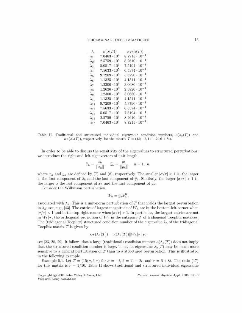
Table II. Traditional and structured individual eigenvalue condition numbers, κ(λh(T )) andκT (λh(T )), respectively, for the matrix T = (15;−i, 11 − 2i, 6 + 8i).

In order to be able to discuss the sensitivity of the eigenvalues to structured perturbations,we introduce the right and left eigenvectors of unit length,

xh =xh

‖xh‖, yh =

yh

‖yh‖, h = 1 : n,

where xh and yh are defined by (7) and (8), respectively. The smaller |σ/τ | < 1 is, the largeris the first component of xh and the last component of yh. Similarly, the larger |σ/τ | > 1 is,the larger is the last component of xh and the first component of yh.

Consider the Wilkinson perturbation,

Wh = yhxHh ,

associated with λh. This is a unit-norm perturbation of T that yields the largest perturbationin λh; see, e.g., [43]. The entries of largest magnitude of Wh are in the bottom-left corner when|σ/τ | < 1 and in the top-right corner when |σ/τ | > 1. In particular, the largest entries are notin Wh|T , the orthogonal projection of Wh in the subspace T of tridiagonal Toeplitz matrices.The (tridiagonal Toeplitz) structured condition number of the eigenvalue λh of the tridiagonalToeplitz matrix T is given by

κT (λh(T )) = κ(λh(T ))‖Wh|T ‖F ;

see [23, 28, 29]. It follows that a large (traditional) condition number κ(λh(T )) does not implythat the structured condition number is large. Thus, an eigenvalue λh(T ) may be much moresensitive to a general perturbation of T than to a structured perturbation. This is illustratedin the following example.

Example 5.1. Let T = (15;σ, δ, τ) for σ = −i, δ = 11 − 2i, and τ = 6 + 8i. The ratio (17)for this matrix is r = 1/10. Table II shows traditional and structured individual eigenvalue



r dF (T(r),NT ) K50,r ‖λ(T(r)) − λ(T ∗(r))‖2

0.1 2.23 · 101 3.79 · 1024 1.16 · 101

0.3 1.73 · 101 1.18 · 1013 5.06 · 100

0.5 1.24 · 101 6.98 · 107 2.12 · 100

0.9 2.47 · 100 2.45 · 102 6.52 · 10−2

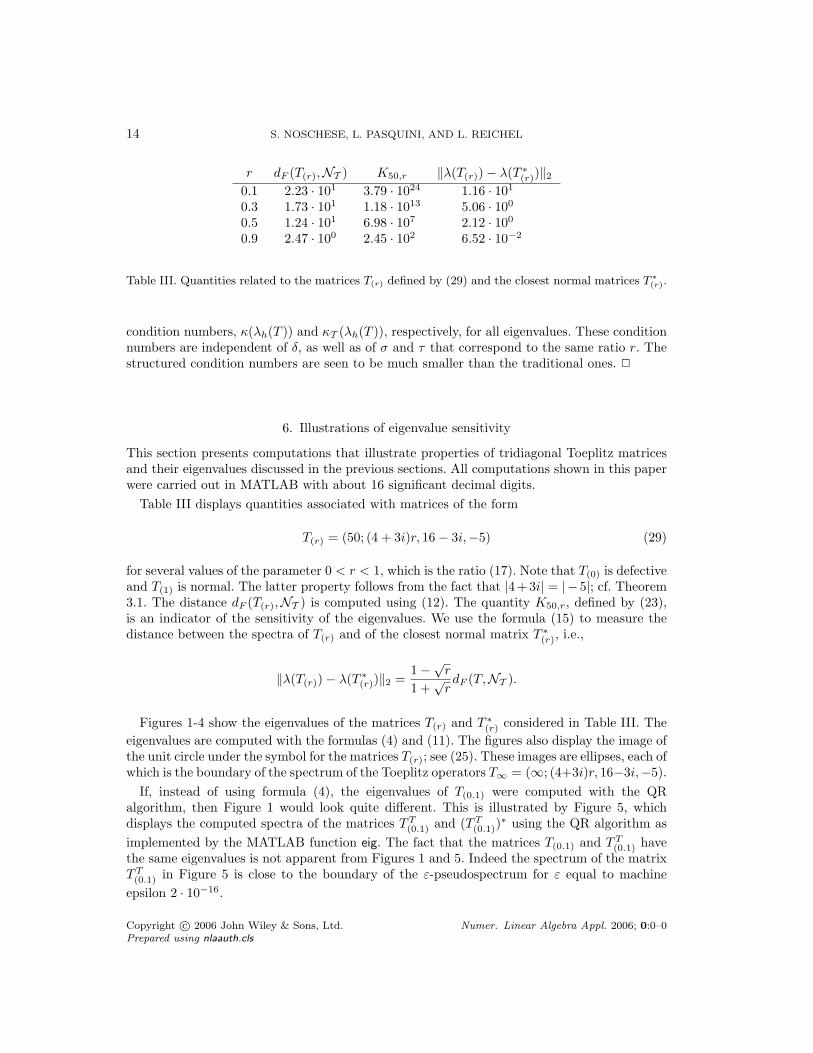
Table III. Quantities related to the matrices T(r) defined by (29) and the closest normal matrices T ∗

(r).

condition numbers, κ(λh(T )) and κT (λh(T )), respectively, for all eigenvalues. These conditionnumbers are independent of δ, as well as of σ and τ that correspond to the same ratio r. Thestructured condition numbers are seen to be much smaller than the traditional ones. 2

6. Illustrations of eigenvalue sensitivity

This section presents computations that illustrate properties of tridiagonal Toeplitz matricesand their eigenvalues discussed in the previous sections. All computations shown in this paperwere carried out in MATLAB with about 16 significant decimal digits.

Table III displays quantities associated with matrices of the form

T(r) = (50; (4 + 3i)r, 16 − 3i,−5) (29)

for several values of the parameter 0 < r < 1, which is the ratio (17). Note that T(0) is defectiveand T(1) is normal. The latter property follows from the fact that |4+3i| = |− 5|; cf. Theorem3.1. The distance dF (T(r),NT ) is computed using (12). The quantity K50,r, defined by (23),is an indicator of the sensitivity of the eigenvalues. We use the formula (15) to measure thedistance between the spectra of T(r) and of the closest normal matrix T ∗

(r), i.e.,

‖λ(T(r)) − λ(T ∗(r))‖2 =

1 −√r

1 +√

rdF (T,NT ).

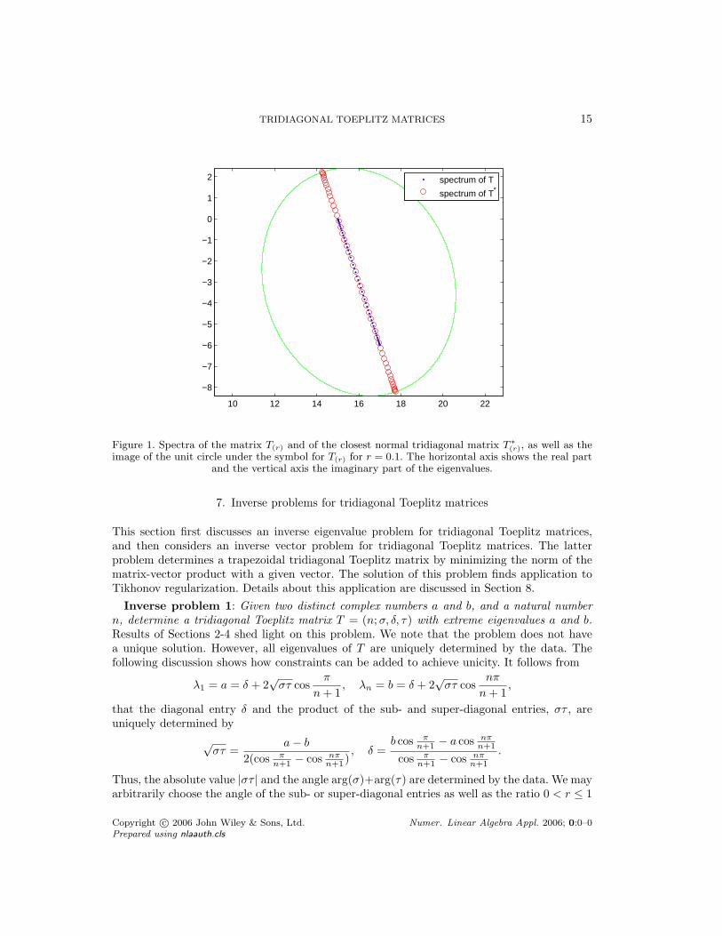
Figures 1-4 show the eigenvalues of the matrices T(r) and T ∗(r) considered in Table III. The

eigenvalues are computed with the formulas (4) and (11). The figures also display the image ofthe unit circle under the symbol for the matrices T(r); see (25). These images are ellipses, each ofwhich is the boundary of the spectrum of the Toeplitz operators T∞ = (∞; (4+3i)r, 16−3i,−5).

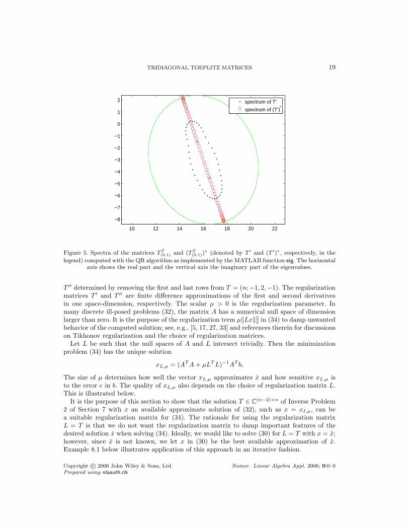
If, instead of using formula (4), the eigenvalues of T(0.1) were computed with the QRalgorithm, then Figure 1 would look quite different. This is illustrated by Figure 5, whichdisplays the computed spectra of the matrices TT

(0.1) and (TT(0.1))

∗ using the QR algorithm as

implemented by the MATLAB function eig. The fact that the matrices T(0.1) and TT(0.1) have

the same eigenvalues is not apparent from Figures 1 and 5. Indeed the spectrum of the matrixTT

(0.1) in Figure 5 is close to the boundary of the ε-pseudospectrum for ε equal to machine

epsilon 2 · 10−16.



10 12 14 16 18 20 22

−8

−7

−6

−5

−4

−3

−2

−1

0

1

2

spectrum of T

spectrum of T*

Figure 1. Spectra of the matrix T(r) and of the closest normal tridiagonal matrix T ∗

(r), as well as theimage of the unit circle under the symbol for T(r) for r = 0.1. The horizontal axis shows the real part

and the vertical axis the imaginary part of the eigenvalues.

7. Inverse problems for tridiagonal Toeplitz matrices

This section first discusses an inverse eigenvalue problem for tridiagonal Toeplitz matrices,and then considers an inverse vector problem for tridiagonal Toeplitz matrices. The latterproblem determines a trapezoidal tridiagonal Toeplitz matrix by minimizing the norm of thematrix-vector product with a given vector. The solution of this problem finds application toTikhonov regularization. Details about this application are discussed in Section 8.

Inverse problem 1: Given two distinct complex numbers a and b, and a natural numbern, determine a tridiagonal Toeplitz matrix T = (n;σ, δ, τ) with extreme eigenvalues a and b.Results of Sections 2-4 shed light on this problem. We note that the problem does not havea unique solution. However, all eigenvalues of T are uniquely determined by the data. Thefollowing discussion shows how constraints can be added to achieve unicity. It follows from

λ1 = a = δ + 2√

στ cosπ

n + 1, λn = b = δ + 2

√στ cos

nπ

n + 1,

that the diagonal entry δ and the product of the sub- and super-diagonal entries, στ , areuniquely determined by

√στ =

a − b

2(cos πn+1 − cos nπ

n+1 ), δ =

b cos πn+1 − a cos nπ

n+1

cos πn+1 − cos nπ

n+1

.

Thus, the absolute value |στ | and the angle arg(σ)+arg(τ) are determined by the data. We mayarbitrarily choose the angle of the sub- or super-diagonal entries as well as the ratio 0 < r ≤ 1



10 12 14 16 18 20 22

−8

−6

−4

−2

0

2

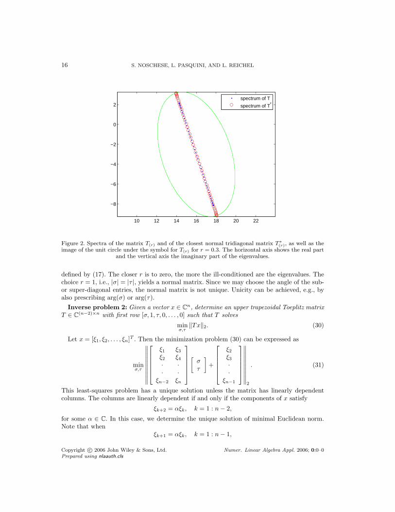
spectrum of T

spectrum of T*




defined by (17). The closer r is to zero, the more the ill-conditioned are the eigenvalues. Thechoice r = 1, i.e., |σ| = |τ |, yields a normal matrix. Since we may choose the angle of the sub-or super-diagonal entries, the normal matrix is not unique. Unicity can be achieved, e.g., byalso prescribing arg(σ) or arg(τ).

Inverse problem 2: Given a vector x ∈ Cn, determine an upper trapezoidal Toeplitz matrix

T ∈ C(n−2)×n with first row [σ, 1, τ, 0, . . . , 0] such that T solves

minσ,τ

‖Tx‖2. (30)

Let x = [ξ1, ξ2, . . . , ξn]T . Then the minimization problem (30) can be expressed as

minσ,τ

∥∥∥∥∥∥∥∥∥∥

ξ1 ξ3

ξ2 ξ4

· ·· ·

ξn−2 ξn

[στ

]+

ξ2

ξ3

··

ξn−1

∥∥∥∥∥∥∥∥∥∥2

. (31)

This least-squares problem has a unique solution unless the matrix has linearly dependentcolumns. The columns are linearly dependent if and only if the components of x satisfy

ξk+2 = αξk, k = 1 : n − 2,

for some α ∈ C. In this case, we determine the unique solution of minimal Euclidean norm.Note that when

ξk+1 = αξk, k = 1 : n − 1,



8 10 12 14 16 18 20 22 24−10

−8

−6

−4

−2

0

2

4

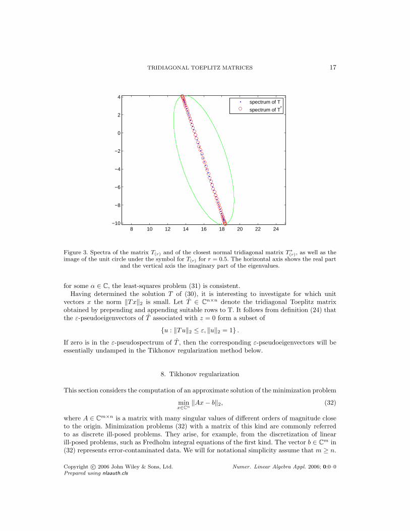
spectrum of T

spectrum of T*




for some α ∈ C, the least-squares problem (31) is consistent.Having determined the solution T of (30), it is interesting to investigate for which unit

vectors x the norm ‖Tx‖2 is small. Let T ∈ Cn×n denote the tridiagonal Toeplitz matrix

obtained by prepending and appending suitable rows to T. It follows from definition (24) thatthe ε-pseudoeigenvectors of T associated with z = 0 form a subset of

u : ‖Tu‖2 ≤ ε, ‖u‖2 = 1 .

If zero is in the ε-pseudospectrum of T , then the corresponding ε-pseudoeigenvectors will beessentially undamped in the Tikhonov regularization method below.

8. Tikhonov regularization

This section considers the computation of an approximate solution of the minimization problem

minx∈Cn

‖Ax − b‖2, (32)

where A ∈ Cm×n is a matrix with many singular values of different orders of magnitude close

to the origin. Minimization problems (32) with a matrix of this kind are commonly referredto as discrete ill-posed problems. They arise, for example, from the discretization of linearill-posed problems, such as Fredholm integral equations of the first kind. The vector b ∈ C

m in(32) represents error-contaminated data. We will for notational simplicity assume that m ≥ n.



5 10 15 20 25−12

−10

−8

−6

−4

−2

0

2

4

6

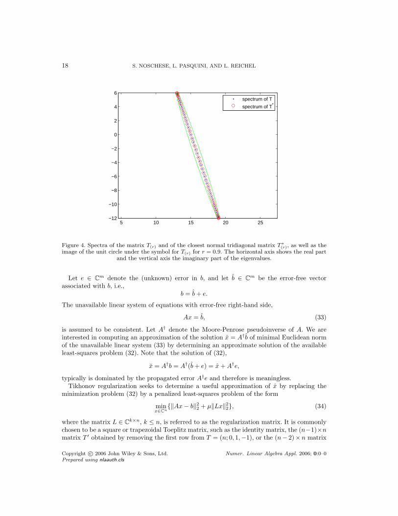
spectrum of T

spectrum of T*




Let e ∈ Cm denote the (unknown) error in b, and let b ∈ C

m be the error-free vectorassociated with b, i.e.,

b = b + e.

The unavailable linear system of equations with error-free right-hand side,

Ax = b, (33)

is assumed to be consistent. Let A† denote the Moore-Penrose pseudoinverse of A. We areinterested in computing an approximation of the solution x = A†b of minimal Euclidean normof the unavailable linear system (33) by determining an approximate solution of the availableleast-squares problem (32). Note that the solution of (32),

x = A†b = A†(b + e) = x + A†e,

typically is dominated by the propagated error A†e and therefore is meaningless.Tikhonov regularization seeks to determine a useful approximation of x by replacing the

minimization problem (32) by a penalized least-squares problem of the form

minx∈Cn

‖Ax − b‖22 + µ‖Lx‖2

2, (34)

where the matrix L ∈ Ck×n, k ≤ n, is referred to as the regularization matrix. It is commonly

chosen to be a square or trapezoidal Toeplitz matrix, such as the identity matrix, the (n−1)×nmatrix T ′ obtained by removing the first row from T = (n; 0, 1,−1), or the (n− 2)×n matrix



10 12 14 16 18 20 22

−8

−7

−6

−5

−4

−3

−2

−1

0

1

2

spectrum of T’

spectrum of (T’)*

Figure 5. Spectra of the matrices T T(0.1) and (T T

(0.1))∗ (denoted by T ′ and (T ′)∗, respectively, in the

legend) computed with the QR algorithm as implemented by the MATLAB function eig. The horizontalaxis shows the real part and the vertical axis the imaginary part of the eigenvalues.

T ′′ determined by removing the first and last rows from T = (n;−1, 2,−1). The regularizationmatrices T ′ and T ′′ are finite difference approximations of the first and second derivativesin one space-dimension, respectively. The scalar µ > 0 is the regularization parameter. Inmany discrete ill-posed problems (32), the matrix A has a numerical null space of dimensionlarger than zero. It is the purpose of the regularization term µ‖Lx‖2

2 in (34) to damp unwantedbehavior of the computed solution; see, e.g., [5, 17, 27, 33] and references therein for discussionson Tikhonov regularization and the choice of regularization matrices.

Let L be such that the null spaces of A and L intersect trivially. Then the minimizationproblem (34) has the unique solution

xL,µ = (AT A + µLT L)−1AT b,

The size of µ determines how well the vector xL,µ approximates x and how sensitive xL,µ isto the error e in b. The quality of xL,µ also depends on the choice of regularization matrix L.This is illustrated below.

It is the purpose of this section to show that the solution T ∈ C(n−2)×n of Inverse Problem

2 of Section 7 with x an available approximate solution of (32), such as x = xI,µ, can bea suitable regularization matrix for (34). The rationale for using the regularization matrixL = T is that we do not want the regularization matrix to damp important features of thedesired solution x when solving (34). Ideally, we would like to solve (30) for L = T with x = x;however, since x is not known, we let x in (30) be the best available approximation of x.Example 8.1 below illustrates application of this approach in an iterative fashion.



We assume that an estimate δ of ‖e‖ is available. This allows us to determine theregularization parameter µ with the aid of the discrepancy principle. Specifically, we chooseµ > 0 so that

‖AxL,µ − b‖2 = δ; (35)

however, we remark that other approaches to determine µ also can be used, such as the L-curveand generalized cross validation; see, e.g., [17].

We will solve (34) for a general matrix L by using the generalized singular valuedecomposition (GSVD) of the matrix pair A,L. It is then easy to determine µ from thenonlinear equation (35). When L = I, the generalized singular value decomposition can bereplaced by the (standard) singular value decomposition (SVD); see, e.g., Hansen [17] fordetails on the applications of the GSVD or SVD to the solution of (34).

0 20 40 60 80 100 120 140 160 180 2000

0.05

0.1

0.15

0.2

0.25

0 20 40 60 80 100 120 140 160 180 2000.06

0.08

0.1

0.12

0.14

0.16

0.18

0.2

(a) (b)

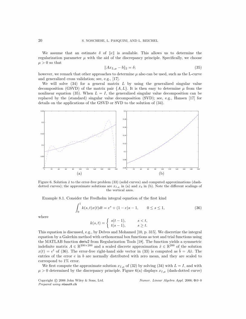
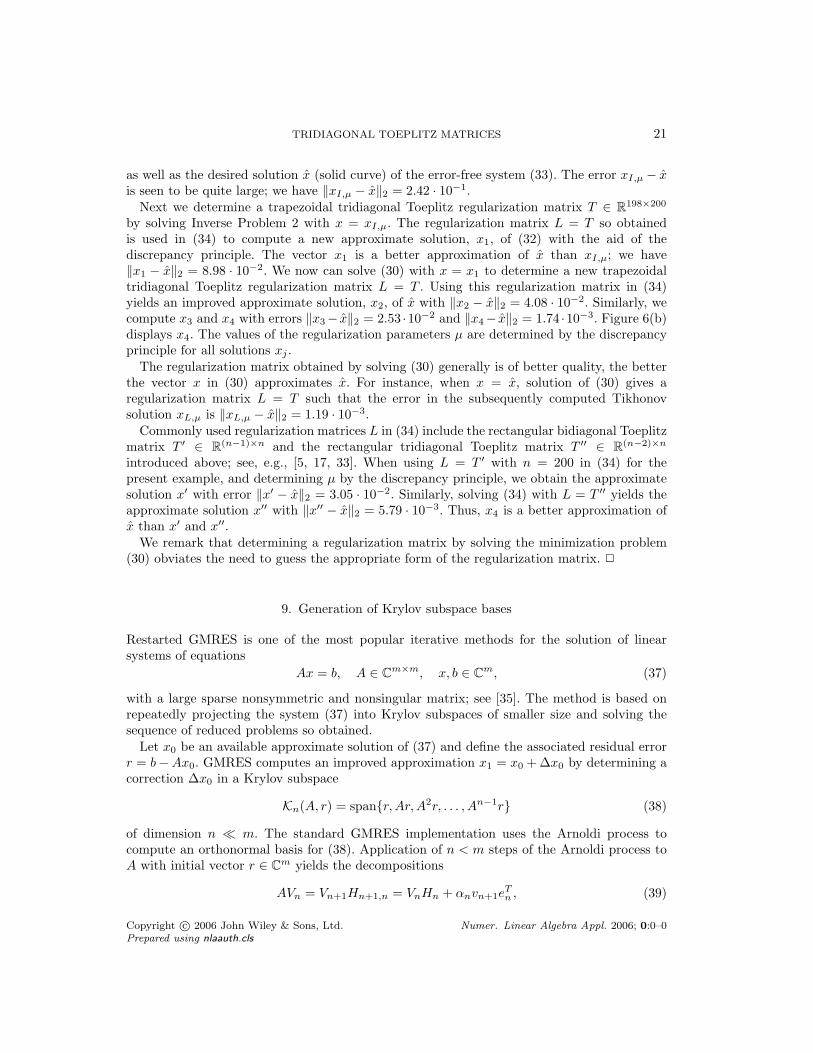
Figure 6. Solution x to the error-free problem (33) (solid curves) and computed approximations (dash-dotted curves); the approximate solutions are xI,µ in (a) and x4 in (b). Note the different scalings of

the vertical axes.

Example 8.1. Consider the Fredholm integral equation of the first kind∫ 1

0

k(s, t)x(t)dt = es + (1 − e)s − 1, 0 ≤ s ≤ 1, (36)

where

k(s, t) =

s(t − 1), s < t,t(s − 1), s ≥ t.

This equation is discussed, e.g., by Delves and Mohamed [10, p. 315]. We discretize the integralequation by a Galerkin method with orthonormal box functions as test and trial functions usingthe MATLAB function deriv2 from Regularization Tools [18]. The function yields a symmetricindefinite matrix A ∈ R

200×200 and a scaled discrete approximation x ∈ R200 of the solution

x(t) = et of (36). The error-free right-hand side vector in (33) is computed as b = Ax. Theentries of the error e in b are normally distributed with zero mean, and they are scaled tocorrespond to 1% error.

We first compute the approximate solution xI,µ of (32) by solving (34) with L = I, and withµ > 0 determined by the discrepancy principle. Figure 6(a) displays xI,µ (dash-dotted curve)



as well as the desired solution x (solid curve) of the error-free system (33). The error xI,µ − xis seen to be quite large; we have ‖xI,µ − x‖2 = 2.42 · 10−1.

Next we determine a trapezoidal tridiagonal Toeplitz regularization matrix T ∈ R198×200

by solving Inverse Problem 2 with x = xI,µ. The regularization matrix L = T so obtainedis used in (34) to compute a new approximate solution, x1, of (32) with the aid of thediscrepancy principle. The vector x1 is a better approximation of x than xI,µ; we have‖x1 − x‖2 = 8.98 · 10−2. We now can solve (30) with x = x1 to determine a new trapezoidaltridiagonal Toeplitz regularization matrix L = T . Using this regularization matrix in (34)yields an improved approximate solution, x2, of x with ‖x2 − x‖2 = 4.08 · 10−2. Similarly, wecompute x3 and x4 with errors ‖x3− x‖2 = 2.53 ·10−2 and ‖x4− x‖2 = 1.74 ·10−3. Figure 6(b)displays x4. The values of the regularization parameters µ are determined by the discrepancyprinciple for all solutions xj .

The regularization matrix obtained by solving (30) generally is of better quality, the betterthe vector x in (30) approximates x. For instance, when x = x, solution of (30) gives aregularization matrix L = T such that the error in the subsequently computed Tikhonovsolution xL,µ is ‖xL,µ − x‖2 = 1.19 · 10−3.

Commonly used regularization matrices L in (34) include the rectangular bidiagonal Toeplitzmatrix T ′ ∈ R

(n−1)×n and the rectangular tridiagonal Toeplitz matrix T ′′ ∈ R(n−2)×n

introduced above; see, e.g., [5, 17, 33]. When using L = T ′ with n = 200 in (34) for thepresent example, and determining µ by the discrepancy principle, we obtain the approximatesolution x′ with error ‖x′ − x‖2 = 3.05 · 10−2. Similarly, solving (34) with L = T ′′ yields theapproximate solution x′′ with ‖x′′ − x‖2 = 5.79 · 10−3. Thus, x4 is a better approximation ofx than x′ and x′′.

We remark that determining a regularization matrix by solving the minimization problem(30) obviates the need to guess the appropriate form of the regularization matrix. 2

9. Generation of Krylov subspace bases

Restarted GMRES is one of the most popular iterative methods for the solution of linearsystems of equations

Ax = b, A ∈ Cm×m, x, b ∈ C

m, (37)

with a large sparse nonsymmetric and nonsingular matrix; see [35]. The method is based onrepeatedly projecting the system (37) into Krylov subspaces of smaller size and solving thesequence of reduced problems so obtained.

Let x0 be an available approximate solution of (37) and define the associated residual errorr = b−Ax0. GMRES computes an improved approximation x1 = x0 + ∆x0 by determining acorrection ∆x0 in a Krylov subspace

Kn(A, r) = spanr,Ar,A2r, . . . , An−1r (38)

of dimension n ≪ m. The standard GMRES implementation uses the Arnoldi process tocompute an orthonormal basis for (38). Application of n < m steps of the Arnoldi process toA with initial vector r ∈ C

m yields the decompositions

AVn = Vn+1Hn+1,n = VnHn + αnvn+1eTn , (39)



where the columns of Vn form an orthonormal basis for (38) and Hn+1,n ∈ C(n+1)×n is an

upper Hessenberg matrix. The matrix Hn ∈ Cn×n is obtained by removing the last row of

Hn+1,n and the vector vn+1 is the last columns of Vn+1.The correction ∆x0 = Vny of x0 is the solution of the least-squares problem

min∆x0∈Kn(A,r)

‖A∆x0 − r‖2 = miny∈Cn

‖Hn+1,ny − e1‖b‖2 ‖2.

Due to storage and work considerations, n generally is chosen much smaller than m; in manyapplications 20 ≤ n ≤ 50. Therefore, the computed approximate solution x1 of (37) typicallyis not of desired accuracy. One then seeks to determine an improved approximate solutionx2 = x1 +∆x1 by determining a correction ∆x1 in (38) with r = b−Ax1. The vector ∆x1 canbe computed similarly as ∆x0, i.e., by application of n steps of the Arnoldi process. Generally,several corrections ∆xj have to be computed until a sufficiently accurate approximate solutionof (37) has been found.

The Arnoldi process determines one column of the matrix Vn at a time. Each new column isorthogonalized against all already available columns by the modified Gram-Schmidt method.This makes it difficult to achieve high performance on parallel computers. Therefore, the use ofnonorthogonal Krylov subspace bases, that circumvent the sequential orthogonalization of theArnoldi process and lend themselves better to efficient implementation on parallel computers,has received considerable attention; see, e.g., [2, 14, 21, 22, 32, 36]. We remark that the basisin (38) generally cannot be used, because for many matrices A it is very ill-conditioned; in factthe vectors Ajb in (38) may be numerically linearly dependent already for n of modest size.

We would like to use a Krylov subspace basis that is easy to construct and is numericallylinearly independent in finite precision arithmetic. Krylov subspace bases based on translatedand scaled Chebyshev polynomials p0, p1, p2, . . . of the first kind, that are orthogonal withrespect to an inner product on some interval in the complex plane,

S = tz1 + (1 − t)z2 : 0 ≤ t ≤ 1, z1, z2 ∈ C, z1 6= z2, (40)

are convenient to use; see [21, 22, 32] and references therein. Here pj is a polynomial of degreej. One can evaluate the basis

p0(A)r, p1(A)r, . . . , pn−1(A)r (41)

for (38) without sequential orthogonalization, by using the three-term recursion formula forthe pj . Subsequent orthogonalization of the basis (41) by QR factorization of the matrixwith columns pj(A)r, 0 ≤ j < n, can be carried out efficiently on a parallel computer; see[4, 21, 22, 32] for discussions. The computations require the vectors (41) to be numericallylinearly independent. This is typically satisfied with an appropriate choice of the interval (40);see [21, 32] for analyses. The polynomials are scaled so that the vectors pj(A)r are of unitlength.

A suitable interval (40) for defining the translated and scaled Chebyshev polynomials oftencan be determined from the spectrum of the matrix Hn computed by the Arnoldi process (39)when computing the initial correction ∆x0. A common approach described in the literature,see, e.g., [21, 22, 32] and references therein, is to determine the smallest ellipse that containsthe spectrum of Hn, and let z1 and z2 be the foci of this ellipse. The translated Chebyshevpolynomials associated with the interval (40), suitable scaled, are used in all subsequent restartsuntil a sufficiently accurate approximate solution of (37) has been found. The use of bases of the



form (41) sidesteps the need to apply the Arnoldi process in restarts and yields an algorithmthat is well suited for implementation on parallel computers; see, e.g., [22, 32] for discussions.

However, the determination of the smallest ellipse that contains a given point set is a fairlycomplicated computational task. We describe two ways, based on properties of tridiagonalToeplitz matrices, to simplify the computations. First we transform Hn to a similar non-Hermitian tridiagonal matrix Tn by application of the non-Hermitian Lanczos process to Hn

with initial vectors e1. Our first approach to determine a suitable interval (40) is to solve theminimization problem

minT∈T

‖T − Tn‖F (42)

for the matrix T = (n;σ, δ, τ). We then let (40) be the line segment (6) determined by T . Thesecomputations are very simple. Since the spectrum of T is explicitly known, the smallest intervalcontaining all eigenvalues can be determined accurately also when T is highly nonnormal.

Alternatively, we may determine the interval (40) by using the field of values of Tn, definedby

W(Tn) =

xHTnx

xHx, x ∈ C

n\0

.

Let T = (n;σ, δ, τ) be the solution of (42). We now determine a region in C that containsW(Tn) as follows; see [31] for further details. The closest normal tridiagonal Toeplitz matrixto Tn, denoted by T ∗, is the normal tridiagonal Toeplitz matrix closest to T . Therefore,

W(T ∗) =

δ + t ei(arg σ+arg τ)/2 : t ∈ R, |t| ≤ (|σ| + |τ |) cos

π

n + 1

; (43)

cf. Corollary 3.1. Moreover,

W(Tn) ⊂ W(T ∗) + W(Tn − T ∗),

W(Tn − T ∗) ⊂ z ∈ C : |z| ≤ ‖Tn − T ∗‖F .The evaluation of ‖Tn − T ∗‖F is straightforward and so is the computation of a sports field-shaped region R that contains W(Tn). We may let (40) be the interval between the foci of thelargest ellipse that can be inscribed in R or, simpler, the interval (43).

Example 9.1. We illustrate the first approach. Consider the elliptic boundary value problem

−∆u + γ∂u

∂s= f in Ω, (44)

u = 0 on ∂Ω,

where Ω is the unit square in the (s, t)-plane with boundary ∂Ω and γ = 60. We approximate∆ and ∂/∂s by standard 2nd order finite differences, using 38 equidistant interior grid points inboth the s- and t-directions. This yields a nonsymmetric nonsingular matrix A ∈ R

1444×1444,which can be expressed as I⊗T1+T2⊗I, where T1 and T2 are tridiagonal Toeplitz matrices and⊗ denotes Kronecker product. Using (4), one can derive explicit expressions for the eigenvaluesof A; they are allocated in a rectangle that is symmetric with respect to the real axis in C. Welet f ≡ 1.

Figure 7 displays the computed spectrum of the matrix A (blue dots) in the complex plane;the horizontal and vertical axes are the real and imaginary axes, respectively. The computedeigenvalues are not very accurate, because one of the tridiagonal matrices Tj that determine



−4 −2 0 2 4 6 8 10−0.8

−0.6

−0.4

−0.2

0

0.2

0.4

0.6

0.8

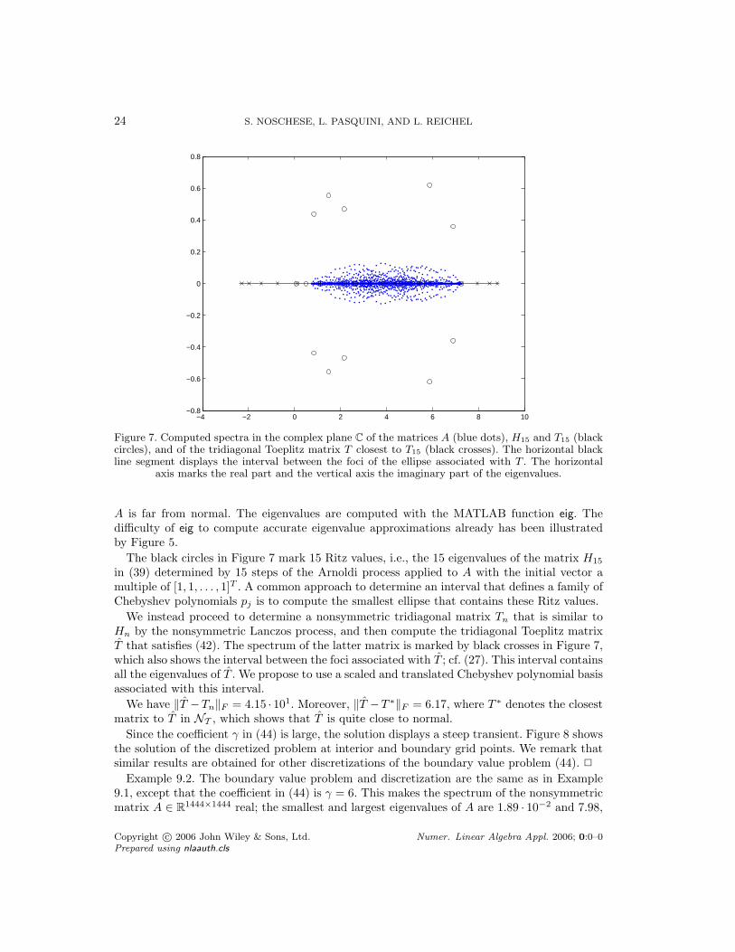
Figure 7. Computed spectra in the complex plane C of the matrices A (blue dots), H15 and T15 (blackcircles), and of the tridiagonal Toeplitz matrix T closest to T15 (black crosses). The horizontal blackline segment displays the interval between the foci of the ellipse associated with T . The horizontal

axis marks the real part and the vertical axis the imaginary part of the eigenvalues.

A is far from normal. The eigenvalues are computed with the MATLAB function eig. Thedifficulty of eig to compute accurate eigenvalue approximations already has been illustratedby Figure 5.

The black circles in Figure 7 mark 15 Ritz values, i.e., the 15 eigenvalues of the matrix H15

in (39) determined by 15 steps of the Arnoldi process applied to A with the initial vector amultiple of [1, 1, . . . , 1]T . A common approach to determine an interval that defines a family ofChebyshev polynomials pj is to compute the smallest ellipse that contains these Ritz values.

We instead proceed to determine a nonsymmetric tridiagonal matrix Tn that is similar toHn by the nonsymmetric Lanczos process, and then compute the tridiagonal Toeplitz matrixT that satisfies (42). The spectrum of the latter matrix is marked by black crosses in Figure 7,which also shows the interval between the foci associated with T ; cf. (27). This interval containsall the eigenvalues of T . We propose to use a scaled and translated Chebyshev polynomial basisassociated with this interval.

We have ‖T −Tn‖F = 4.15 · 101. Moreover, ‖T −T ∗‖F = 6.17, where T ∗ denotes the closestmatrix to T in NT , which shows that T is quite close to normal.

Since the coefficient γ in (44) is large, the solution displays a steep transient. Figure 8 showsthe solution of the discretized problem at interior and boundary grid points. We remark thatsimilar results are obtained for other discretizations of the boundary value problem (44). 2

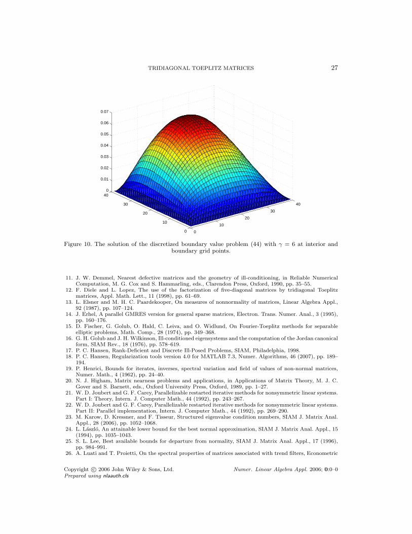
Example 9.2. The boundary value problem and discretization are the same as in Example9.1, except that the coefficient in (44) is γ = 6. This makes the spectrum of the nonsymmetricmatrix A ∈ R

1444×1444 real; the smallest and largest eigenvalues of A are 1.89 · 10−2 and 7.98,



0

10

20

30

40

0

10

20

30

400

0.002

0.004

0.006

0.008

0.01

0.012

0.014

0.016

Figure 8. The solution of the discretized boundary value problem (44) with γ = 60 at interior andboundary grid points.

respectively.

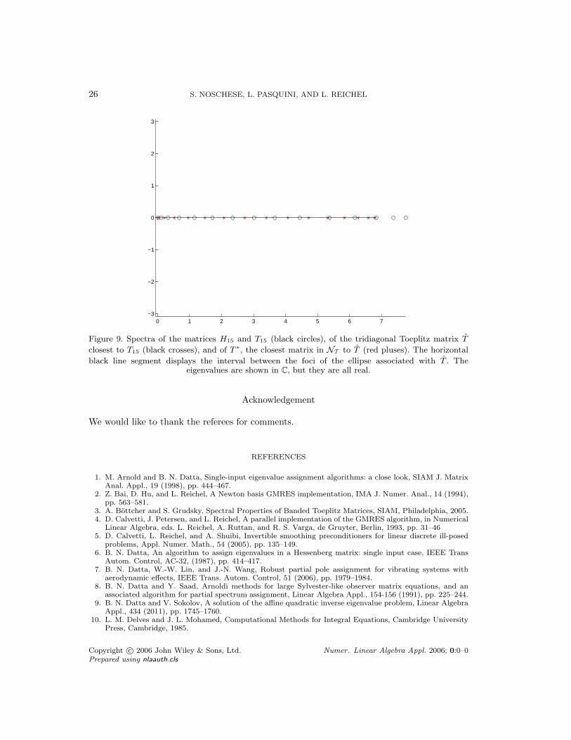
Figure 9 shows 15 Ritz values of A, i.e., the spectra of the matrices H15 in (39) and of thenonsymmetric tridiagonal matrix T15 (black circles). All Ritz values are seen to be real. Thespectrum of the closest tridiagonal Toeplitz matrix T , i.e., the solution of (42), is displayed byblack crosses. The figure also shows the interval between the foci associated with T ; cf. (27).This interval contains all the eigenvalues of T . We may use a scaled and translated Chebyshevpolynomial basis associated with this interval. Finally, Figure 9 depicts the eigenvalues of theclosest normal tridiagonal Toeplitz matrix T ∗ to T ; they are marked by red plus signs. Wealso can use the interval between the foci of T ∗ to define the translated and scaled Chebyshevpolynomials pj in (41). We have ‖T − Tn‖F = 4.91 and ‖T − T ∗‖F = 1.46 · 10−1.

Figure 10 shows the solution of the discretized problem at interior and boundary grid points.2

10. Conclusion

This paper discusses the conditioning of eigenvalues of tridiagonal Toeplitz matrices. Thesimple structure of these matrices makes it possible to derive simple expressions and boundsfor the individual, global, traditional, and structured condition numbers. This led us to discussseveral applications, including an inverse eigenvalue problem. New applications of tridiagonalToeplitz matrices to the construction of regularization matrices for Tikhonov regularizationand to the construction of Krylov subspace bases are described. These applications are verypromising and will be investigated in more detail in forthcoming work.



0 1 2 3 4 5 6 7−3

−2

−1

0

1

2

3

Figure 9. Spectra of the matrices H15 and T15 (black circles), of the tridiagonal Toeplitz matrix T

closest to T15 (black crosses), and of T ∗, the closest matrix in NT to T (red pluses). The horizontal

black line segment displays the interval between the foci of the ellipse associated with T . Theeigenvalues are shown in C, but they are all real.

Acknowledgement

We would like to thank the referees for comments.

REFERENCES

1. M. Arnold and B. N. Datta, Single-input eigenvalue assignment algorithms: a close look, SIAM J. MatrixAnal. Appl., 19 (1998), pp. 444–467.

2. Z. Bai, D. Hu, and L. Reichel, A Newton basis GMRES implementation, IMA J. Numer. Anal., 14 (1994),pp. 563–581.

3. A. Bottcher and S. Grudsky, Spectral Properties of Banded Toeplitz Matrices, SIAM, Philadelphia, 2005.4. D. Calvetti, J. Petersen, and L. Reichel, A parallel implementation of the GMRES algorithm, in Numerical

Linear Algebra, eds. L. Reichel, A. Ruttan, and R. S. Varga, de Gruyter, Berlin, 1993, pp. 31–465. D. Calvetti, L. Reichel, and A. Shuibi, Invertible smoothing preconditioners for linear discrete ill-posed

problems, Appl. Numer. Math., 54 (2005), pp. 135–149.6. B. N. Datta, An algorithm to assign eigenvalues in a Hessenberg matrix: single input case, IEEE Trans

Autom. Control, AC-32, (1987), pp. 414–417.7. B. N. Datta, W.-W. Lin, and J.-N. Wang, Robust partial pole assignment for vibrating systems with

aerodynamic effects, IEEE Trans. Autom. Control, 51 (2006), pp. 1979–1984.8. B. N. Datta and Y. Saad, Arnoldi methods for large Sylvester-like observer matrix equations, and an

associated algorithm for partial spectrum assignment, Linear Algebra Appl., 154-156 (1991), pp. 225–244.9. B. N. Datta and V. Sokolov, A solution of the affine quadratic inverse eigenvalue problem, Linear Algebra

Appl., 434 (2011), pp. 1745–1760.10. L. M. Delves and J. L. Mohamed, Computational Methods for Integral Equations, Cambridge University

Press, Cambridge, 1985.



0

10

20

30

40

0

10

20

30

400

0.01

0.02

0.03

0.04

0.05

0.06

0.07

Figure 10. The solution of the discretized boundary value problem (44) with γ = 6 at interior andboundary grid points.

11. J. W. Demmel, Nearest defective matrices and the geometry of ill-conditioning, in Reliable NumericalComputation, M. G. Cox and S. Hammarling, eds., Clarendon Press, Oxford, 1990, pp. 35–55.

12. F. Diele and L. Lopez, The use of the factorization of five-diagonal matrices by tridiagonal Toeplitzmatrices, Appl. Math. Lett., 11 (1998), pp. 61–69.

13. L. Elsner and M. H. C. Paardekooper, On measures of nonnormality of matrices, Linear Algebra Appl.,92 (1987), pp. 107–124.

14. J. Erhel, A parallel GMRES version for general sparse matrices, Electron. Trans. Numer. Anal., 3 (1995),pp. 160–176.

15. D. Fischer, G. Golub, O. Hald, C. Leiva, and O. Widlund, On Fourier-Toeplitz methods for separableelliptic problems, Math. Comp., 28 (1974), pp. 349–368.

16. G. H. Golub and J. H. Wilkinson, Ill-conditioned eigensystems and the computation of the Jordan canonicalform, SIAM Rev., 18 (1976), pp. 578–619.

17. P. C. Hansen, Rank-Deficient and Discrete Ill-Posed Problems, SIAM, Philadelphia, 1998.18. P. C. Hansen, Regularization tools version 4.0 for MATLAB 7.3, Numer. Algorithms, 46 (2007), pp. 189–

194.19. P. Henrici, Bounds for iterates, inverses, spectral variation and field of values of non-normal matrices,

Numer. Math., 4 (1962), pp. 24–40.20. N. J. Higham, Matrix nearness problems and applications, in Applications of Matrix Theory, M. J. C.

Gover and S. Barnett, eds., Oxford University Press, Oxford, 1989, pp. 1–27.21. W. D. Joubert and G. F. Carey, Parallelizable restarted iterative methods for nonsymmetric linear systems.

Part I: Theory, Intern. J. Computer Math., 44 (1992), pp. 243–267.22. W. D. Joubert and G. F. Carey, Parallelizable restarted iterative methods for nonsymmetric linear systems.

Part II: Parallel implementation, Intern. J. Computer Math., 44 (1992), pp. 269–290.23. M. Karow, D. Kressner, and F. Tisseur, Structured eigenvalue condition numbers, SIAM J. Matrix Anal.

Appl., 28 (2006), pp. 1052–1068.24. L. Laszlo, An attainable lower bound for the best normal approximation, SIAM J. Matrix Anal. Appl., 15

(1994), pp. 1035–1043.25. S. L. Lee, Best available bounds for departure from normality, SIAM J. Matrix Anal. Appl., 17 (1996),

pp. 984–991.26. A. Luati and T. Proietti, On the spectral properties of matrices associated with trend filters, Econometric



Theory, 26 (2010), pp. 1247–1261.27. S. Morigi, L. Reichel, and F. Sgallari, A truncated projected SVD method for linear discrete ill-posed

problems, Numer. Algorithms, 43 (2006), pp. 197–213.28. S. Noschese and L. Pasquini, Eigenvalue condition numbers: zero-structured versus traditional, J. Comput.

Appl. Math., 185 (2006), pp. 174–189.29. S. Noschese and L. Pasquini, Eigenvalue patterned condition numbers: Toeplitz and Hankel cases, J.

Comput. Appl. Math., 206 (2007), pp. 615–624.30. S. Noschese, L. Pasquini, and L. Reichel, The structured distance to normality of an irreducible real

tridiagonal matrix, Electron. Trans. Numer. Anal., 28 (2007), pp. 65–77.31. S. Noschese and L. Reichel, The structured distance to normality of banded Toeplitz matrices, BIT, 49

(2009), pp. 629–640.32. B. Philippe and L. Reichel, On the generation of Krylov subspace bases, Appl. Numer. Math., in press.33. L. Reichel and Q. Ye, Simple square smoothing regularization operators, Electron. Trans. Numer. Anal.,

33 (2009), pp. 63–83.34. L. Reichel and L. N. Trefethen, Eigenvalues and pseudo-eigenvalues of Toeplitz matrices, Linear Algebra

Appl., 162-164 (1992), pp. 153–185.35. Y. Saad, Iterative Methods for Sparse Linear Systems, 2nd ed., SIAM, Philadelphia, 2003.36. R. B. Sidje, Alternatives to parallel Krylov subspace basis computation, Numer. Linear Algebra Appl., 4

(1997), pp. 305–331.37. G. D. Smith, Numerical Solution of Partial Differential Equations, 2nd ed., Clarendon Press, Oxford, 1978.38. L. Smithies, The structured distance to nearly normal matrices, Electron. Trans. Numer. Anal., 36 (2010),

pp. 99–112.39. G. W. Stewart and J. Sun, Matrix Perturbation Theory, Academic Press, London, 1990.40. L. N. Trefethen and M. Embree, Spectra and Pseudospectra, Princeton University Press, Princeton, 2005.41. W.-C. Yueh and S. S. Cheng, Explicit eigenvalues and inverses of tridiagonal Toeplitz matrices with four

perturbed corners, ANZIAM J., 49 (2008), pp. 361–387.42. J. H. Wilkinson, The Algebraic Eigenvalue Problem, Clarendon Press, Oxford, 1965.43. J. H. Wilkinson, Sensitivity of eigenvalues II, Util. Math., 30 (1986), pp. 243–286.


tridiagonal toeplitz matrices: properties and novel ...reichel/publications/toep3.pdf ·...

Documents