trigonometric graphs and models
TRANSCRIPT

Chapter Outline
2.1 Graphs of the Sine andCosine Functions 78
2.2 Graphs of the Tangentand CotangentFunctions 96
2.3 Transformations andApplications ofTrigonometricGraphs 114
2.4 Trigonometric Models131
Trigonometric Graphsand Models
PreviewWhile written records of trigonometry are much more recent that thoseof geometry and algebra, the roots of trigonometry are likely just asancient. Peering into the night-time heavens, ancient scholars noticedpatterns among the celestial bodies, giving rise to the desire to modeltheir regular reoccurrence. But even at the beginning of the modernage, with the tools of geometry at hand and the study of algebramaturing, astronomers were unable to come up with accurate models.This had to wait for the study of periodic functions to mature. Via thepopular media, many people have an awareness of sinusoidal
graphs like the image shown on the oscilloscope in the figure, and abasic understanding of cycles, periods, and wave phenomenon.
Chapter 2
77
cob10054_ch02_77-158.qxd 10/12/06 4:43 PM Page 77 CONFIRMING PAGES

CHAPTER 2 Trigonometric Graphs and Models 2–278
2.1 Graphs of the Sine and Cosine FunctionsINTRODUCTION
As with the graphs of other functions, trigonometric graphs contribute a great dealtoward the understanding of each trig function and its applications. For now, ourprimary interest is the general shape of each basic graph and some of the transfor-mations that can be applied. We will also learn to analyze each graph, and to capi-talize on the features that enable us to apply the functions as real-world models. Fora review of graphical transformations, see Appendix II.
LEARNING OBJECTIVES
In Section 2.1 you will learn how to:
A. Graph usingstandard values andsymmetry
B. Graph usingstandard values andsymmetry
C. Graph sine and cosinefunctions with variousamplitudes and periods
D. Investigate graphs of thereciprocal functions
and
E. Write the equation for agiven graph
f(t) � sec(Bt)f(t) � csc(Bt)
f(t) � cos t
f(t) � sin t
P O I N T O F I N T E R E S T
The close of the third century B.C. marked the end of the glory years of Grecian
mathematics. Lacking the respect his predecessors had for math, science, and art,
Ptolemy VII exiled all scholars who would not swear loyalty to him. As things
turned out, Alexandria’s loss was the rest of Asia Minor’s gain, and mathematical
and scientific knowledge spread. According to one Athenaeus of Naucratis, “The
king sent many Alexandrians into exile, filling the islands and towns with . . . philol-
ogists, philosophers, mathematicians, musicians, painters, physicians and other
professional men. The refugees, reduced by poverty to teaching what they knew,
instructed many other men.”
A. Graphing
From our work in previous sections, we have the values for in the interval
shown in Table 2.1.c0, �
2d
y � sin t
f(t) � sin t
▼
Observe that in this interval (representingQuadrant I), sine values are increasing from
0 to 1. From to (Quadrant II), standard values
taken from the unit circle show sine values aredecreasing from 1 to 0, but through the same out-put values as in QI. See Figures 2.1 through 2.3.
With this information we can extend ourtable of values through noting that sin � � 0�,
��
2
Table 2.1
(�1, 0) (1, 0)
(0, 1)
x
y�� , �2
12
√3
2�3
(�1, 0) (1, 0)
(0, 1)
x
y
3�4
�� , �2√2
2√2
(�1, 0) (1, 0)
(0, 1)
x
y
5�6
2√3
21�� , �
Figure 2.1
Figure 2.2 Figure 2.3
sin a2�
3b �
13
2
sin a3�
4b �
12
2sin a5�
6b �
1
2
t 0
0 113
2
12
2
1
2sin t
�
2
�
3
�
4
�
6
cob10054_ch02_77-158.qxd 10/12/06 4:43 PM Page 78 CONFIRMING PAGES

2–3 Section 2.1 Graphs of the Sine and Cosine Functions 79
(see Table 2.2). Note that both the table and unit circle show the range of the sinefunction is y � 3�1, 1 4 .
Table 2.2
Using the symmetry of the circle and the fact that y is negative in QIII and QIV,we can complete the table for values between and 2�.�
t 0
0 1 01
2
12
2
13
2
13
2
12
2
1
2sin t
�5�
6
3�
4
2�
3
�
2
�
3
�
4
�
6
▼EXAMPLE 1 Use the symmetry of the unit circle and reference arcs of stan-dard values to complete Table 2.3.
Solution: Symmetry shows that for any odd multiple of function
values will be depending on the quadrant of the terminal
side. Similarly, for any reference arc of while for
a reference arc of . With these, we complete the
table as shown in Table 2.4.
sin t � �13
2
�
3,
sin t � �1
2,
�
6,
�12
2
t ��
4,
Table 2.4
NOW TRY EXERCISES 7 AND 8 ▼
Noting that and we plot these points and
connect them with a smooth curve to graph for The first fiveplotted points are labeled in Figure 2.4.
t � 30, 2� 4 .y � sin t
13
2� 0.87,
12
2� 0.71,
1
2� 0.5,
Table 2.3
t
sin t
2�11�
6
7�
4
5�
3
3�
2
4�
3
5�
4
7�
6�
t
0 0�1
2�12
2�13
2�1�
13
2�12
2�
1
2sin t
2�11�
6
7�
4
5�
3
3�
2
4�
3
5�
4
7�
6�
cob10054_ch02_77-158.qxd 10/12/06 4:43 PM Page 79 CONFIRMING PAGES

CHAPTER 2 Trigonometric Graphs and Models 2–480
Expanding the table from to using reference arcs and the unit circle
shows that function values begin to repeat. For example, since
since and so on. Functions that cycle through
a set pattern of values are said to be periodic functions.
�r ��
4,�r �
�
6; sin a9�
4b � sin a�
4b
sin a13�
6b � sin a�
6b
4�2�
sin t
1
Decreasing
�2
Increasing
� 3�2
t2�
�1
�0.5
0.5
(0, 0)
�6� , 0.5� �
4� , 0.71��3� , 0.87�
�2� , 1�
Figure 2.4
PERIODIC FUNCTIONS
A function f is said to be periodic if there is a positive number Psuch that for all t in the domain. The smallestnumber P for which this occurs is called the period of f.
f 1t � P2 � f 1t2
For the sine function we have as in
and with the idea extending to all other real
numbers t: for all integers k. The sine function is periodic withperiod
Although we initially focused on positive values of t in and are certainly possibilities and we note the graph of extends infinitely inboth directions (see Figure 2.5).
y � sin tk 6 030, 2� 4 , t 6 0
P � 2�.sin t � sin1t � 2�k2
sin a9�
4b � sin a�
4� 2�b,sin a�
6� 2�b
sin a13�
6b �sin t � sin1t � 2�2,
Figure 2.5
y � sin t
t
y
�0.5
�1
1
0.5
4��2����
4�3 �
2�3 �
�3
�3 3 3
�� , �12� �
� , 12� �
cob10054_ch02_077-095.qxd 11/22/06 10:36 AM Page 80

2–5 Section 2.1 Graphs of the Sine and Cosine Functions 81
From Figure 2.5 we also note that is an odd function. For instance, we
have and in general for all As
a handy reference, the following box summarizes the main characteristics of using features discussed here and ideas from Section 1.4.
y � sin t
t � R.sin1�t2 � �sin t�sin a�
2b � �1sin a��
2b �
y � sin t
CHARACTERISTICS OF
Unit CircleDefinition Domain Symmetry Maximum values Increasing:
Odd: at
Period Range Zeroes Minimum values Decreasing:
at t � a�
2,
3�
2bt �
3�
2� 2�ksin t � �1t � k�, k � Zy � 3�1, 1 42�
t � 10, 2�2a3�
2, 2�bt � a0,
�
2b ´�
2� 2�kt �sin t � 1� �sin tsin1�t2t � Rsin t � y
t � 10, 2�2f(t) � sin t
Many of the transformations applied to algebraic graphs can also be applied totrigonometric graphs (see Appendix II). These transformations may stretch, reflect,or translate the graph, but it will still retain its basic shape. In numerous applica-tions it will help if you’re able to draw a quick, accurate sketch of the transforma-tions involving To assist this effort, we’ll begin with the standard inter-val combine the characteristics just listed with some simple geometry,and offer the following four-step process. Steps I through IV are illustrated inFigures 2.6 through 2.9.
Step I: Draw the y-axis, mark zero halfway up, with and 1 an equaldistance from this zero. Then draw an extended t-axis and tick mark
to the extreme right.
Step II: Mark halfway between the y-axis and and label it “ ” mark
halfway between on either side and label the marks and
Halfway between these you can draw additional tick marks to repre-
sent the remaining multiples of
Step III: Next, lightly draw a rectangular frame, which we’ll call the referencerectangle, units wide and 2 units tall, centered on the t-axisand with the y-axis along one side.
Step IV: Knowing is positive and increasing in QI; that the range is[�1, 1]; that the zeroes are 0, and and that maximum andminimum values occur halfway between the zeroes (since there is nohorizontal shift), we can draw a reliable graph of by parti-tioning the reference rectangle into four equal parts to locate thezeroes and max/min values. We will call this partitioning of the ref-erence rectangle the rule of fourths, since we are then scaling the
t-axis in increments of .P
4
y � sin t
2�;�,y � sin t
P � 2�
�
4.
3�
2.
�
2�
�,2�
2�
�1
t � 30, 2� 4 , f 1t2 � sin t.
cob10054_ch02_77-158.qxd 10/12/06 4:43 PM Page 81 CONFIRMING PAGES

▼
CHAPTER 2 Trigonometric Graphs and Models 2–682
t
y
�1
1
02� t
y
�1
1
03�2
�2
� 2�
t
y
�1
1
03�2
�2
� 2�
Increasing Decreasing
t
y
�1
1
03�2
�2
� 2�
Figure 2.6
Figure 2.8 Figure 2.9
Figure 2.7
EXAMPLE 2 Use steps I through IV to draw a sketch of for
.
Solution: Begin by completing steps Iand II, then extend the t-axis
to include Beginning at
draw a reference rectangle
2 units high and wide (cen-tered on the x-axis), ending
at The zeroes still occur at and with the max/min
values spaced equally between and on either side (rule of fourths). Plotthese points and connect them with a smooth curve (see the figure).
t � �,t � 03�
2.
2�
��
2,
��
2.
t � c��
2,
3�
2d
y � sin t
Increasing Decreasing
t
y
�1
1
3�2
�2
��2�
NOW TRY EXERCISES 9 AND 10 ▼
B. Graphing
With the graph of established, sketching the graph of is a verynatural next step. First, note that when so the graph of
will begin at (0, 1) in the interval Second, we’ve seen
and are all points on the unit circle since they satisfy
Since and the equation can be
obtained by direct substitution. This means if then and vice
versa, with the signs taken from the appropriate quadrant. The table of values for cosinethen becomes a simple extension of the table for sine, as shown in Table 2.5 fort � 30, � 4 .
cos t � �13
2sin t � �
1
2,
cos2t � sin2t � 1sin t � y,cos t � xx 2 � y2 � 1.
�12
2ba�12
2,a�13
2, �
1
2b
a�1
2, �13
2b,30, 2� 4 .
y � cos tcos t � 1t � 0,f 1t2 � cos tf 1t2 � sin t
f(t) � cos t
I.
III.
II.
IV.
cob10054_ch02_77-158.qxd 10/12/06 4:44 PM Page 82 CONFIRMING PAGES
2–7 Section 2.1 Graphs of the Sine and Cosine Functions 83
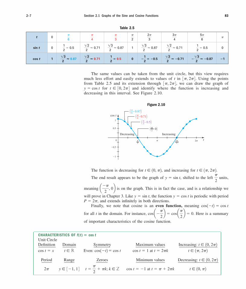
The same values can be taken from the unit circle, but this view requiresmuch less effort and easily extends to values of t in Using the pointsfrom Table 2.5 and its extension through we can draw the graph of
for and identify where the function is increasing anddecreasing in this interval. See Figure 2.10.
t � 30, 2� 4y � cos t3�, 2� 4 , 3�, 2� 4 .
Table 2.5
cos t
1
Decreasing
0 �2
Increasing
� 3�2
t2�
�1
�0.5
0.5
�3� , 0.5�
�2� , 0�
�4� , 0.71�
�6� , 0.87�
Figure 2.10
The function is decreasing for and increasing for .
The end result appears to be the graph of shifted to the left units,
meaning is on the graph. This is in fact the case, and is a relationship we
will prove in Chapter 3. Like the function is periodic with periodand extends infinitely in both directions.
Finally, we note that cosine is an even function, meaning
for all t in the domain. For instance, Here is a summary
of important characteristics of the cosine function.
cos a��
2b � cos a�
2b � 0.
cos1�t2 � cos tP � 2�,
y � cos ty � sin t,
a��
2, 0b
�
2y � sin t,
t � 1�, 2�2t � 10, �2,
t 0
0 1 0
1 0 �1�132
� �0.87122
� �0.71�12
� �0.512
� 0.5122
� 0.71132
� 0.87cos t
1
2� 0.5
12
2� 0.71
13
2� 0.87
13
2� 0.87
12
2� 0.71
1
2� 0.5sin t
�5�
6
3�
4
2�
3
�
2
�
3
�
4
�
6
CHARACTERISTICS OF f(t) �Unit CircleDefinition Domain Symmetry Maximum values Increasing:
Even: at
Period Range Zeroes Minimum values Decreasing:
at t � 10, �2t � � � 2�kcos t � �1k � Zt ��
2� �k;y � 3�1, 1 42�
t � 10, 2�2t � 1�, 2�2t � 2�kcos t � 1cos tcos1�t2�t � Rcos t � x
t � 10, 2�2cos t
cob10054_ch02_77-158.qxd 10/12/06 4:44 PM Page 83 CONFIRMING PAGES

▼
CHAPTER 2 Trigonometric Graphs and Models 2–884
▼EXAMPLE 3Draw a sketch of for
Solution: Using steps I through IV (frame, scaling, zeroes, and max/min
values) produces this graph for in Note the
reference rectangle goes from to ( units in length), and
the graph was then extended to the interval c��, 3�
2d .
2����
c��, 3�
2d .y � cos t
t � c��, 3�
2d .y � cos t
Increasing
Decreasing
t
y
�1
1
�0�� �2
3�2
�2�
y � cos t
NOW TRY EXERCISES 11 AND 12 ▼
C. Graphing and
In many applications, trig functions have maximum and minimum values other than1 and and periods other than For instance, in tropical regions the maximumand minimum temperatures may vary by no more than while for desert regionsthis difference may be or more. This variation is modeled by the amplitude ofsine and cosine functions.
Amplitude and the Coefficient A (B � 1)
For functions of the form and let M represent the Maximum
value and m the minimum value of the functions. Then the quantity gives
the average value of the function, while gives the amplitude of the function.
Amplitude is the maximum displacement from the average value in the positiveor negative direction. It is represented by with A playing a role similar to thatseen for algebraic graphs vertically stretches or compresses the graph of f,and reflects it across the t-axis if Graphs of the form (and
) can quickly be sketched with any amplitude by noting that the zeroesof the function remain fixed (since implies and that the max-imum and minimum values are A and �A respectively (since or implies or Connecting the points that result with a smooth curvewill complete the graph.
�A2.A sin t � A�1sin t � 1
A sin t � 02,sin t � 0y � cos t
y � sin tA 6 02.1Af 1x2�A�,
M � m
2
M � m
2
y � A cos t,y � A sin t
40°20°,
2�.�1,
y � A cos(Bt)y � A sin(Bt)W O R T H Y O F N OT E
Note that the equations and both indicate y is afunction of t, with no reference tothe unit circle definitions and sin t � y.
cos t � x
y � A cos ty � A sin t
EXAMPLE 4 Draw a sketch of for
Solution: This graph has the same zeroes as but the maximum
value is with a minimum value of4 sin a�2b � 4112 � 4,
y � sin t,
t � 30, 2� 4 .y � 4 sin t
cob10054_ch02_77-158.qxd 10/12/06 4:44 PM Page 84 CONFIRMING PAGES

2–9 Section 2.1 Graphs of the Sine and Cosine Functions 85
Zeroes remainfixed
y � 4 sin t
y � sin t
t
�4
4
� 2��2
3�2
NOW TRY EXERCISES 13 THROUGH 18 ▼
Period and the Coefficient B
While basic sine and cosine functions have a period of in many applications theperiod may be very long (tsunami’s) or very short (electromagnetic waves). For theequations and the period depends on the value of B.To see why, consider the function and Table 2.6. Multiplying input val-ues by 2 means each cycle will be completed twice as fast. The table shows that
completes a full cycle in giving a period of (Figure 2.11,red graph).
P � �30, � 4 ,y � cos(2t)
y � cos(2t)y � A cos(Bt),y � A sin(Bt)
2�,
Table 2.7
Dividing input values by 2 (or multiplying by will cause the function to com-plete a cycle only half as fast, doubling the time required to complete a fullcycle. Table 2.7 shows completes only one-half cycle in (Figure 2.11,blue graph).
2�y � cos A12 tB12)
Table 2.6
t 0
2t 0
1 0 0 1�1cos (2t)
2�3�
2�
�
2
�3�
4
�
2
�
4
t 0
0
1 0.92 0.38 0 �1�0.92�22
2�0.38
22
2cos a1
2tb
�7�
8
3�
4
5�
8
�
2
3�
8
�
4
�
8
12
t
2�7�
4
3�
2
5�
4�
3�
4
�
2
�
4
(the amplitude is . Connecting
these points with a “sine curve” gives the graph shown is also shown for comparison).
(y � sin t
�A� � 4241�12 � �44 sin a3�
2b�
cob10054_ch02_77-158.qxd 10/12/06 4:44 PM Page 85 CONFIRMING PAGES

CHAPTER 2 Trigonometric Graphs and Models 2–1086
To sketch these functions for periods other than , we still use a reference rect-angle of height 2A and length P, then break the enclosed t-axis in four equal parts tohelp find and graph the zeroes and max/min values. In general, if the period is “verylarge” one full cycle is appropriate for the graph. If the period is very small, graph at leasttwo cycles.
Note the value of B in Example 5 includes a factor of . This actually happensquite frequently in applications of the trig functions.
�
2�
PERIOD FORMULA FOR SINE AND COSINE
For B a real number and functions and
the period is given by P �2�
B.
y � A cos1Bt2,y � A sin1Bt2▼EXAMPLE 5 Draw a sketch of for
Solution: The amplitude is so the reference rectangle will beunits high. Since the graph will be vertically
reflected across the t-axis. The period is (note the
factors of reduce to 1), so the frame will be 5 units in length.Breaking the t-axis into four parts within the frame gives
units, indicating that we should scale the t-axis in multiples of In cases where the factor reduces, we scale the t-axis as a “stan-dard” number line, and estimate the location of multiples of Forpractical reasons, we first draw the unreflected graph (shown inblue) for guidance in drawing the reflected graph.
�.�
14.5
4
A14B 5 ��
P �2�
0.4�� 5
A 6 02122 � 4�A� � 2,
t � 3��, 2� 4 .y � �2 cos10.4�t2
y � �2 cos(0.4�t)
y � ��2�cos(0.4�t)
t
y
�2
�1
2
1
1 2 3 4 5 6�3 �2 �1
�� � 2�
NOW TRY EXERCISES 19 THROUGH 30 ▼
The graphs of and shown in Figure 2.11clearly illustrate this relationship and howthe value of B affects the period of a graph.
To find the period for arbitrary values
of B, the formula is used. Note for
and as
shown. For and 4�.P �2�
1�2�B �
1
2,y � cos a1
2 tb,
P �2�
2� �,B � 2,y � cos12t2,
P �2�
B
y � cosA12 tB y � cos(2t),y � cos t, Figure 2.11
y � cos ty � cos(2t)y
y � cos� t�12
t
�1
1
� 2� 3� 4�
cob10054_ch02_77-158.qxd 10/12/06 4:44 PM Page 86 CONFIRMING PAGES

2–11 Section 2.1 Graphs of the Sine and Cosine Functions 87
▼
D. Graphs of and
The graphs of these reciprocal functions follow quite naturally from the graphs ofand by using these observations: (1) you cannot divide
by zero, (2) the reciprocal of a very small number is a very large number (and viceversa), and (3) the reciprocal of 1 is 1. Just as with rational functions, division by
zero creates a vertical asymptote, so the graph of will have a
vertical asymptote at every point where This occurs at where kis an integer Further, the graph of willshare the maximums and minimums of since the reciprocal of 1 and
are still 1 and Finally, due to observation 2, the graph of the cosecantfunction will be increasing when the sine function is decreasing, and decreasingwhen the sine function is increasing. In most cases, we graph by draw-ing a sketch of then using the preceding observations as demonstratedin Example 6. In doing so, we discover that the period of the cosecant function isalso 2�.
y � sin1Bt2, y � csc1Bt2�1.�1
y � sin1Bt2, y � csc1Bt2��, 0, �, 2�, . . .2.1. . . �2�,t � �k,sin t � 0.
y � csc t �1
sin t
y � A cos1Bt2,y � A sin1Bt2y � sec(Bt)y � csc(Bt)
EXAMPLE 6 Graph the function for
Solution: The related sine function is which means we’ll draw a rectangular frame units high.
The period is so the reference frame will be units in length. Breaking the t-axis
into four parts within the frame means each tick mark will be units apart, with the
asymptotes occurring at 0, and A partial table and the resulting graph are shown.2�.�,
a1
4b a2�
1b�
�
2
2�P �2�
1� 2�,
2A � 2y � sin t,
t � 30, 4� 4 .y � csc t
y � csc (t)
t
y
�1
1• Vertical asymptoteswhere sine is zero
• Shares maximum andminimum valueswith sine
• Output values are reciprocated
��2
3�2
5�2
7�2
2� 3� 4�
NOW TRY EXERCISES 31 AND 32 ▼
Similar observations can be made regarding and its relationship to(see Exercises 8, 33, and 34). The most important characteristics of the
cosecant and secant functions are summarized in the following box. For these func-tions, there is no discussion of amplitude, and no mention is made of their zeroessince neither graph intersects the t-axis.
y � cos1Bt2 y � sec1Bt2
t
0 0 S undefined
1 1�
2
213� 1.15
13
2� 0.87
�
3
212� 1.41
12
2� 0.71
�
4
2
1� 2
1
2� 0.5
�
6
1
0
csc tsin t
cob10054_ch02_77-158.qxd 10/12/06 4:44 PM Page 87 CONFIRMING PAGES

CHAPTER 2 Trigonometric Graphs and Models 2–1288
E. Writing Equations from Graphs
Mathematical concepts are best reinforced by working with them in both “forwardand reverse.” Where graphs are concerned, this means we should attempt to find theequation of a given graph, rather than only using an equation to sketch the graph.Exercises of this type require that you become very familiar with the graph’s basiccharacteristics and how each is expressed as part of the equation.
▼EXAMPLE 7 The graph shown here is of the form Find thevalue of A and B.
Solution: By inspection, the graph has an amplitude of and a period of
To find B we used the period formula substituting
for P and solving.
period formula
substitute for P
multiply by 2B
solve for B
The result is which gives us the equation y � 2 sinA43 tB.B � 43,
B �4
3
3�B � 4�
3�
2 3�
2�
2�
B
P �2�
B
3�
2
P �2�
B,P �
3�
2.
A � 2
y � A sin1Bt2.
y � A sin(Bt)
y
t
�2
2
� 2��2
��2
3�2
There are a number of interesting applications of this “graph to equation”process in the exercise set. See Exercises 59 to 70.
CHARACTERISTICS OF and
Unit Circle Unit CircleDefinition Period Definition Period
Domain Range Domain Range
y � 1�q, �1 4 ´ 31, q 2t ��
2� �ky � 1�q, �1 4 ´ 31, q 2t � k�
2�sec t �1x
2�csc t �1y
y � sec ty � csc ty � sec ty � csc t
NOW TRY EXERCISES 35 THROUGH 56 ▼
cob10054_ch02_77-158.qxd 10/12/06 4:44 PM Page 88 CONFIRMING PAGES

2–13 Section 2.1 Graphs of the Sine and Cosine Functions 89
TECHNOLOGY H IGHLIGHT
Exploring Amplitudes and PeriodsThe keystrokes shown apply to a TI-84 Plus model.
Please consult your manual or our Internet site for
other models.
In practice, trig applications offer an immense
range of coefficients, creating amplitudes that are
sometimes very large and sometimes extremely
small, as well as periods ranging from nanoseconds,
to many years. This Technology Highlight is
designed to help you use the calculator more effec-
tively in the study of these functions. To begin, we
note the Plus offers
a preset option
that automatically
sets a window size
convenient to many
trig graphs. The
resulting after
pressing 7:ZTrigis shown in Figure 2.12
for a calculator set in Radian .
One important concept of Section 2.1 is that a
change in amplitude will not change the location
of the zeroes or max/min values. On the
screen, enter
and then
use 7:ZTrig to
graph the functions.
As you see in Figure
2.13, each graph rises
to the expected ampli-
tude, while “holding
on” to the zeroes
(graph the functions
in Simultaneous ).
To explore concepts related to the coefficient B
and its effect on the period of a trig function,
enter and on the
screen and graph using 7:ZTrig. While the
result is “acceptable,” the graphs are difficult to
read and compare, so we manually change the
window size to obtain a better view (Figure 2.14).
Y2 � sin12x2Y1 � sin a12
xb
Y4 � 4 sin x,
Y3 � 2 sin x,Y2 � sin x,Y1 �1
2 sin x,
TI-84
After pressing
we can use
and the up or down
arrows to help
identify each
function.
A true test of
effective calculator
use comes when the
amplitude or period is
a very large or very
small number. For
instance, the tone you
hear while pressing
“5“ on your
telephone is actually
a combination of the
tones modeled by and
Graphing these functions
requires a careful analysis of the period, otherwise
the graph can appear either garbled, misleading, or
difficult to read—try graphing on the
7:ZTrig or 6:ZStandard screens (see
Figure 2.15). First note the amplitude is
and the period is or With a period
this short, even graphing the function from
to gives a distorted graph.
Setting Xmin to
Xmax to
and Xscl
to gives the
graph in Figure 2.16,
which can be used to
investigate characteris-
tics of the function.
Exercise 1: Graph the
second tone mentioned here and
find its value at sec.
Exercise 2: Graph the function
on a “friendly” window and find the value at
x � 550.
Y1 � 950 sin10.005t2t � 0.00025
Y2 � sin 32�113362t 4
11/7702�10
1�770,
�1�770,
Xmax � 1Xmin � �1
1
770.P �
2�
2�770
A � 1,
Y1
Y2 � sin 32�113362t 4 .Y1 � sin 32�17702t 4
Figure 2.12
Figure 2.13
ZOOM
ZOOM
WINDOW
Figure 2.15
Figure 2.16
Figure 2.14
MODE
Y�
ZOOM
MODE
Y�
ZOOM
TRACE
GRAPH
ZOOM
ZOOM
cob10054_ch02_77-158.qxd 10/12/06 4:44 PM Page 89 CONFIRMING PAGES
CHAPTER 2 Trigonometric Graphs and Models 2–1490
3. For the sine and cosine functions, thedomain is and the range is
.
2.1 E X E R C I S E S
CONCEPTS AND VOCABULARY
Fill in each blank with the appropriate word or phrase. Carefully reread the section if needed.
1. For the sine function, output values
are in the interval c 0, �
2d .
2. For the cosine function, output values are
in the interval c 0, �
2d .
4. The amplitude of sine and cosine is de-fined to be the maximum from the value in the pos-itive and negative directions.
5. Discuss/describe the four-step processoutlined in this section for the graphingof basic trig functions. Include aworked-out example and a detailedexplanation.
6. Discuss/explain how you would deter-mine the domain and range ofWhere is this function undefined? Why?Graph using
What do you notice?y � 2 cos12t2.y � 2 sec 12t2y � sec x.
DEVELOPING YOUR SKILLS
7. Use the symmetry of the unit circle and reference arcs of standard values to complete atable of values for in the interval
8. Use the standard values for for to create a table of values foron the same interval.
Use steps I through IV given in this section to draw a sketch of
9. for 10. for
11. for 12. for
Use a reference rectangle and the rule of fourths to draw an accurate sketch of thefollowing functions through two complete cycles—one where and one where
Clearly state the amplitude and period as you begin.
13. 14. 15.
16. 17. 18.
19. 20. 21.
22. 23. 24.
25. 26. 27.
28. 29. 30.
Draw the graph of each function by first sketching the related sine and cosine graphs, andapplying the observations made in this section.
31. 32.
33. 34. f 1t2 � 3 sec 12t2y � 2 sec t
g1t2 � 2 csc 14t2y � 3 csc t
g1t2 � 3 cos1184�t2f 1t2 � 2 sin 1256�t2y � 2.5 cos a2�
5tb
y � 4 sin a5�
3 tbg1t2 � 5 cos18�t2f 1t2 � 3 sin 14�t2
y � �3 cos a3
4 tbf 1t2 � 4 cos a1
2 tby � 1.7 sin 14t2
y � 0.8 cos12t2y � �cos12t2y � �sin 12t2y �
3
4 sin ty �
1
2 sin ty � �3 cos t
y � �2 cos ty � 4 sin ty � 3 sin t
t 6 0.t 7 0,
t � c��
2,
5�
2dy � cos tt � c��
2, 2� dy � cos t
t � 3��, � 4y � sin tt � c�3�
2,
�
2dy � sin t
y � sec tt � 3�, 2� 4y � cos t
t � 3�, 2� 4 .y � cos t
cob10054_ch02_77-158.qxd 10/17/06 2:04 PM Page 90CONFIRMING PAGES

2–15 Exercises 91
Clearly state the amplitude and period of each function, then match it with the correspond-ing graph.
35. 36. 37.
38. 39. 40.
41. 42. 43.
44. 45. 46.
a. b.
c. d.
e. f.
g. h. i.
j. k. l.
The graphs shown are of the form or Use the characteristicsillustrated for each graph to determine its equation.
47. 48. 49.
�0.4
�0.8
0.4
0 t
0.8y
2� 4� 6�
�4
�8
4
0 15
25
35
45
1 t
8y
�0.5
�1
0.5
0
1
�
8�
2�
43�
85�
8t
y
y � A csc 1Bt2.y � A cos1Bt2
�1
�2
1
0
2
�
4�
23�
4�
y
t
�1
�2
1
0
2
�
4�
23�
4� t
y
�2
�4
2
0 t
4y
112
16
14
13
512
�2
�4
2
0 t
4y
112
16
14
13
512
�2
�4
2
0 2� 4� 6� 8� t
4y
�2
�4
2
0 2� 4� 6� 8� t
4y
�2
�4
2
0 �
23�
22�� t
4y
�2
�4
2
0 �
23�
22�� t
4y
�2
�4
2
0 1144
172
148
136
5144
4
t
y
�2
�4
2
0 1144
172
148
136
5144
t
4y
4� 5� 6�3�2�
�1
�2
1
0
2
�
y
t4� 5�3�2�
�1
�2
1
0
2
�
y
t
y � 4 cos172�t2y � 4 sin 1144�t2y � csc 112�t2y � sec 18�t2g1t2� 7
4 cos10.8t2f 1t2 �
3
4 cos 10.4t2
y � 2 sec a1
4 tby � 2 csc a1
2tby � �3 cos12t2
y � 3 sin 12t2y � 2 sin 14t2y � �2 cos14t2
cob10054_ch02_77-158.qxd 10/12/06 4:44 PM Page 91 CONFIRMING PAGES
50. 51. 52.
Match each graph to its equation, then graphically estimate the points of intersection. Con-firm or contradict your estimate(s) by substituting the values into the given equations usinga calculator.
53. 54.
55. 56.
WORKING WITH FORMULAS
57. The Pythagorean theorem in trigonometric form:
The formula shown is commonly known as a Pythagorean identity and is introducedmore formally in Chapter 3. It is derived by noting that on a unit circle, and
while Given that use the formula to find the valueof in Quadrant I. What is the Pythagorean triple associated with these values ofx and y?
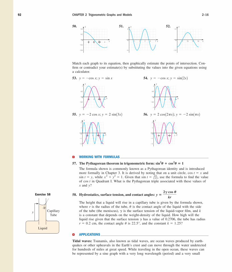
58. Hydrostatics, surface tension, and contact angles:
The height that a liquid will rise in a capillary tube is given by the formula shown,where r is the radius of the tube, is the contact angle of the liquid with the sideof the tube (the meniscus), is the surface tension of the liquid-vapor film, and kis a constant that depends on the weight-density of the liquid. How high will theliquid rise given that the surface tension has a value of 0.2706, the tube has radius
cm, the contact angle is and the constant ?
APPLICATIONS
Tidal waves: Tsunamis, also known as tidal waves, are ocean waves produced by earth-quakes or other upheavals in the Earth’s crust and can move through the water undetectedfor hundreds of miles at great speed. While traveling in the open ocean, these waves canbe represented by a sine graph with a very long wavelength (period) and a very small
k � 1.2522.5°,�r � 0.2g
g
�
y �2� cos �
kr
cos tsin t � 15
113,x 2 � y2 � 1.sin t � y,
cos t � x
sin2� � cos2� � 1
�1
�2
1
0 32
2
2
12
1 x
y
�1
�2
1
0 �
23�
2� 2� x
2y
y � �2 sin 1�x 2y � 2 cos12�x 2;y � 2 sin 13x 2y � �2 cos x;
�0.5
�1
0.5
0�
23�
2� 2�
x
1y
�0.5
�1
0.5
0 �
23�
2� 2�
1
x
y
y � sin 12x 2y � �cos x;y � sin xy � �cos x;
�1.2
0 � 2� t
1.2y
3� 4�
�6
0 1 2 3 4 5
6y
t
�0.2
�0.4
0.2
0 �
4�
23�
4� t
0.4y
CHAPTER 2 Trigonometric Graphs and Models 2–1692
y CapillaryTube
Liquid
�
Exercise 58
cob10054_ch02_77-158.qxd 10/12/06 4:44 PM Page 92 CONFIRMING PAGES

amplitude. Tsunami waves only attain a monstrous size as they approach the shore, andrepresent a very different phenomenon than the ocean swells created by heavy winds overan extended period of time.
59. A graph modeling a tsunami wave is given in the figure.(a) What is the height of the tsunami wave (from crest totrough)? Note that is considered the level of a calmocean. (b) What is the tsunami’s wavelength? (c) Find theequation for this wave.
60. A heavy wind is kicking up ocean swells approximately 10 fthigh (from crest to trough), with wavelengths of 250 ft.(a) Find the equation that models these swells. (b) Graph theequation. (c) Determine the height of a wave measured 200 ftfrom the trough of the previous wave.
Sinusoidal models: The sine and cosine functions are of great importance to meteorologicalstudies, as when modeling the temperature based on the time of day, the illumination of theMoon as it goes through its phases, or even the prediction of tidal motion.
61. The graph given shows the deviation from the average dailytemperature for the hours of a given day, with corre-sponding to 6 A.M. (a) Use the graph to determine the relatedequation. (b) Use the equation to find the deviation at (5 P.M.) and confirm that this point is on the graph. (c) If theaverage temperature for this day was what was thetemperature at midnight?
62. The equation models the height of the tide along a certain coastal area, as
compared to average sea level. Assuming is midnight, (a) graph this function overa 12-hr period. (b) What will the height of the tide be at 5 A.M.? (c) Is the tide rising or fallingat this time?
Sinusoidal movements: Many animals exhibit a wavelike motion in their movements, asin the tail of a shark as it swims in a straight line or the wingtips of a large bird in flight.Such movements can be modeled by a sine or cosine function and will vary depending onthe animal’s size, speed, and other factors.
63. The graph shown models the position of a shark’s tail at timet, as measured to the left (negative) and right (positive) of astraight line along its length. (a) Use the graph to determinethe related equation. (b) Is the tail to the right, left, or at cen-ter when sec? How far? (c) Would you say the sharkis “swimming leisurely,” or “chasing its prey”? Justify your answer.
64. The State Fish of Hawaii is the humuhumunukunukuapua’a, a small colorful fish foundabundantly in coastal waters. Suppose the tail motion of an adult fish is modeled by theequation with d(t) representing the position of the fish’s tail at time t, asmeasured in inches to the left (negative) or right (positive) of a straight line along its length.(a) Graph the equation over two periods. (b) Is the tail to the left or right of center at
sec? How far? (c) Would you say this fish is “swimming leisurely,” or “runningfor cover”? Justify your answer.
Kinetic energy: The kinetic energy a planet possesses as it orbits the Sun can be modeledby a cosine function. When the planet is at its apogee (greatest distance from the Sun), itskinetic energy is at its lowest point as it slows down and “turns around” to head backtoward the Sun. The kinetic energy is at its highest when the planet “whips around the Sun”to begin a new orbit.
t � 2.7
d 1t2 � sin 115�t2
t � 6.5
t � 0
y � 7 sin a�
6 tb
72°,
t � 11
t � 0
h � 0
2–17 Exercises 93
2
1
20 40 60 80 100
Heightin feet
Miles�2
�1
Temperaturedeviation
�2
�4
2
04 8 12 16 20 24
t
4
20
10
1
Distancein inches
t sec
�20
�10 2 3 4 5
cob10054_ch02_77-158.qxd 10/12/06 4:44 PM Page 93 CONFIRMING PAGES

CHAPTER 2 Trigonometric Graphs and Models 2–1894
65. Two graphs are given here. (a) Which of the graphs could represent the kinetic energy ofa planet orbiting the Sun if the planet is at its perigee (closest distance to the Sun) when
? (b) For what value(s) of t does this planet possess 62.5% of its maximum kineticenergy with the kinetic energy increasing? (c) What is the orbital period of this planet?
a. b.
66. The potential energy of the planet is the antipode of its kinetic energy, meaning whenkinetic energy is at 100%, the potential energy is 0%, and when kinetic energy is at 0%the potential energy is at 100%. (a) How is the graph of the kinetic energy related to thegraph of the potential energy? In other words, what transformation could be applied to thekinetic energy graph to obtain the potential energy graph? (b) If the kinetic energy is at62.5% and increasing [as in Graph 65(b)], what can be said about the potential energy inthe planet’s orbit at this time?
Visible light: One of the narrowest bands in the electromagnetic spectrum is the regioninvolving visible light. The wavelengths (periods) of visible light vary from 400 nano-meters (purple/violet colors) to 700 nanometers (bright red). The approximate wavelengthsof the other colors are shown in the diagram.
67. The equations for the colors in this spectrum have the form where
gives the length of the sine wave. (a) What color is represented by the equation
? (b) What color is represented by the equation ?
68. Name the color represented by each of the graphs (a) and (b) here and write therelated equation.
a. b.
Alternating current: Surprisingly, even characteristics of the electric current supplied toyour home can be modeled by sine or cosine functions. For alternating current (AC), theamount of current I (in amps) at time t can be modeled by where A repre-sents the maximum current that is produced, and � is related to the frequency at which thegenerators turn to produce the current.
69. Find the equation of the household current modeled by the graph, then use the equa-tion to determine I when sec. Verify that the resulting ordered pair is onthe graph.
t � 0.045
I � A sin1�t2,
y � sin a �
310 tby � sin a �
240 tb
2�
gy � sin 1gt2,
t � 0
�1
0 150 300 450 600 750 900 1050 1200
1y
t (nanometers)
�1
0 150 300 450 600 750 900 1050 1200
1y
t (nanometers)
25
0
50
75
100
12 48 60 72 84 96
t days
Perc
ent o
f K
E
24 36
25
0
50
75
100
12 48 60 72 84 96
t days
Perc
ent o
f K
E
24 36
Violet Blue Green Yellow Orange Red
400 500 600 700
�30
�15
30
15
Current I
t sec
150
125
350
225
110
Exercise 69
cob10054_ch02_77-158.qxd 10/12/06 4:44 PM Page 94 CONFIRMING PAGES

2–19 Exercises 95
70. If the voltage produced by an AC circuit is modeled by the equation (a) what is the period and amplitude of the related graph? (b) What voltage is producedwhen
WRITING, RESEARCH, AND DECISION MAKING
71. For and the expression gives the average value
of the function, where M and m represent the maximum and minimum values respec-tively. What was the average value of every function graphed in this section? Computea table of values for the function and note its maximum and mini-mum values. What is the average value of this function? What transformation has beenapplied to change the average value of the function? Can you name the average valueof by inspection? How is the amplitude related to this average value?
(Hint: Graph the horizontal line on the same grid.)
72. Use the Internet or the resources of a local library to do some research on tsunamis(see Exercises 59 and 60). Attempt to find information on (a) exactly how they aregenerated; (b) some of the more notable tsunamis in history; (c) the average amplitudeof a tsunami; (d) their average wavelength or period; and (e) the speeds they travel inthe open ocean. Prepare a short summary of what you find.
73. To understand where the period formula came from, consider that if
the graph of completes one cycle from to Ifcompletes one cycle from to Discuss how this
observation validates the period formula.
74. Horizontal stretches and compressions are remarkably similar for all functions. Use agraphing calculator to graph the functions and on a 7:ZTrig screen (graph in bold). Note that completes two periods in the time ittakes to complete 1 period (the graph of is horizontally compressed). Nowenter and substituting 2x for xas before. After graphing these on a 4:ZDecimal screen, what do you notice?How do these algebraic graphs compare to the trigonometric graphs?
EXTENDING THE CONCEPT
75. The tone you hear when pressing the digit “9” on your telephone is actually acombination of two separate tones, which can be modeled by the functions
and Which of the two functions has the shortest period? By carefully scaling the axes, graph the function having the shorterperiod using the steps I through IV discussed in this section.
76. Consider the functions and For one of these functions, theportion of the graph below the x-axis is reflected above the x-axis, creating a series of“humps.” For the other function, the graph obtained for is reflected across the y-axis to form the graph for After a thoughtful contemplation (without actuallygraphing), try to decide which description fits and which fits justifying yourthinking. Then confirm or contradict your guess using a graphing calculator.
MAINTAINING YOUR SKILLS
g1x2,f 1x 2t 6 0.t 7 0
g1x2 � �sin t�.f 1x 2 � sin 1 �t �2
g1t2 � sin 32� 11477 2 t 4 .f 1t2 � sin 32� 1852 2t 4
Y2 � 1 32x 42 � 1 2 1 32x 42 � 4 2,Y1 � 1x 2 � 1 2 1x
2 � 4 2 Y2Y1
Y2Y1
Y2 � sin 12x 2Y1 � sin x
Bt � 2�.Bt � 0y � sin 1Bt2B � 1,1t � 2�.1t � 0y � sin 1Bt2 � sin 11t2
B � 1,P �2�
B
y �M � m
2
y � �2 cos t � 1
y � 2 sin t � 3,
M � m
2y � A cos1Bx 2,y � A sin 1Bx 2
t � 0.2?
E � 155 sin 1120�t2,
ZOOM
ZOOM
77. (1.3) Given sin find an ad-ditional value of t in that makesthe equation true.
78. (1.1) Invercargill, New Zealand, is atsouth latitude. If the Earth
has a radius of 3960 mi, how far isInvercargill from the equator?
46° 14 ¿ 24–sin t � 0.9
30, 2� 21.12 � 0.9,
cob10054_ch02_77-158.qxd 10/12/06 4:44 PM Page 95 CONFIRMING PAGES

2.2 Graphs of the Tangent and Cotangent FunctionsLEARNING OBJECTIVES
In Section 2.2 you will learn how to:
A. Graph usingasymptotes, zeroes, and the
ratio
B. Graph usingasymptotes, zeroes, and the
ratio
C. Identify and discussimportant characteristics of
and
D. Graph andwith various
values of A and B
E. Solve applications ofand y � cot ty � tan t
y � A cot(Bt)y � A tan(Bt)
y � cot ty � tan t
cos t
sin t
y � cot t
sin t
cos t
y � tan t
INTRODUCTION
Unlike the other four trig functions, tangent and cotangent have no maximum orminimum value on any open interval of their domain. However, it is precisely thisunique feature that adds to their value as mathematical models. Collectively, the sixfunctions give scientists the tools they need to study, explore, and investigate a widerange of phenomena, extending our understanding of the world around us.
P O I N T O F I N T E R E S T
The sine and cosine functions evolved from studies of the chord lengths within
a circle and their applications to astronomy. Although we know today they are
related to the tangent and cotangent functions, it appears the latter two devel-
oped quite independently of this context. When time was measured by the length
of the shadow cast by a vertical stick, observers noticed the shadow was
extremely long at sunrise, cast no shadow at noon, and returned to extreme
length at sunset. Records tracking shadow length in this way date back as far as
1500 B.C. in ancient Egypt, and are the precursor of our modern tangent and
cotangent functions.▼
CHAPTER 2 Trigonometric Graphs and Models 2–2096
79. (1.3) Given with (a) find the related values of x, y, and r; (b) state
the quadrant of the terminal side; and (c) give the value of the other five trig functions of t.
80. (1.1) Use a standard triangle to calculate the distance from the ball to the pin on the sev-enth hole, given the ball is in a straight line with the 100-yd plate, as shown in the figure.
tan t 6 0:cos t �28
53
81. (1.1) The Ferris wheel shown has a radius of 25 ft and is turning at a rate of 14 rpm.(a) What is the angular velocity in radians? (b) What distance does a seat on the rim travelas the Ferris wheel turns through an angle of 225�? (c) What is the linear velocity(in miles per hour) of a person sitting in a seat at the rim of the Ferris wheel?
82. (1.2) The world’s tallest unsupported flagpole was erected in 1985 in Vancouver, BritishColumbia. Standing 60 ft from the base of the pole, the angle of elevation is 78�. How tallis the pole?
60�
100 yd
100 yd
Exercise 80 Exercise 81
cob10054_ch02_096-113.qxd 11/22/06 10:34 AM Page 96

2–21 Section 2.2 Graphs of the Tangent and Cotangent Functions 97
A. The Graph of
Like the secant and cosecant functions, tangent is defined in terms of a ratio thatcreates asymptotic behavior at the zeroes of the denominator. In terms of the unit
circle, which means in vertical asymptotes occur at
and , since the x-coordinate on the unit circle is zero. We further note
when the y-coordinate is zero, so the function will have t-intercepts atand in the same interval. This produces the framework for graph-
ing the tangent function shown in Figure 2.17.2�t � ��, 0, �,
tan t � 0
3�
2t �
�
2,
t � ��
2,3��, 2� 4 ,tan t �
yx,
y � tan t
tan t
t3�2
�2
��� 2��2
�2
Asymptotes atodd multiples of
t-intercepts atinteger multiples of �
�2
�1
2
1
�
Knowing the graph must go through these zeroes and approach the asymptotes,we are left with determining the direction of the approach. This can be discoveredby noting that in QI, the y-coordinates of points on the unit circle start at 0 and increase,
while the x-values start at 1 and decrease. This means the ratio defining tan t is
increasing, and in fact becomes infinitely large as t gets very close to A similar
observation can be made for a negative rotation of t in QIV. Using the additional
points provided by and we find the graph of tan t is
increasing throughout the interval and that the function has a period of
We also note is an odd function (symmetric about the origin), sinceas evidenced by the two points just computed. The completed
graph is shown in Figure 2.18 with the primary interval in red.tan1�t2 � �tan t
y � tan t
�.a��
2,
�
2b
tan a�
4b � 1,tan a��
4b � �1
�
2.
y
x
Figure 2.17
�� , 1�
tan t
t3�2
�2
��� 2��2
�4
�2
4
2
�4� , 1�
�4
��
�
Figure 2.18
x
y
(x, y)
(1, 0)(0, 0)
(0, 1)
t
(0, �1)
(�1, 0)
xy
tan t �
cob10054_ch02_77-158.qxd 10/12/06 4:49 PM Page 97 CONFIRMING PAGES

▼
CHAPTER 2 Trigonometric Graphs and Models 2–2298
Table 2.8
EXAMPLE 1Complete Table 2.8 shown for using the values given for sin t and cos t. tan t �
yx
Solution: For the noninteger values of x and y, the “twos will cancel” each time we compute This means we
can simply list the ratio of numerators. The results are shown in Table 2.9.
yx.
Table 2.9
NOW TRY EXERCISES 7 AND 8 ▼
t 0
0 1 0
1 0
tan t �y
x
�1�13
2�12
2�
1
2
1
2
12
2
13
2cos t � x
1
2
12
2
13
2
13
2
12
2
1
2sin t � y
�5�
63�
42�
3�
2�
3�
4�
6
t 0
0 1 0
1 0
0 1 undefined 0�113
�1�1313 � 1.7113
� 0.58tan t �y
x
�1�13
2�12
2�
1
2
1
2
12
2
13
2cos t � x
1
2
12
2
13
2
13
2
12
2
1
2sin t � y
�5�
63�
42�
3�
2�
3�
4�
6
The graph can also be developed by noting the ratio relationship that exists between
sin t, cos t, and tan t. In particular, since and we have
by direct substitution. These and other relationships between the trig
functions will be fully explored in Chapter 3.
tan t �sin t
cos t
tan t �yx,cos t � x,sin t � y,
Additional values can be found using a calculator as needed. For future use andreference, it will help to recognize the approximate decimal equivalent of all standard
values and radian angles. In particular, note that and See
Exercises 9 through 14.
B. The Graph of
Since the cotangent function is also defined in terms of a ratio, it too displaysasymptotic behavior at the zeroes of the denominator, with t-intercepts at the zeroes
y � cot t
113� 0.58.13 � 1.73
cob10054_ch02_77-158.qxd 10/12/06 4:49 PM Page 98 CONFIRMING PAGES
of the numerator. Like the tangent function, can be written in terms of
and and the graph obtained by plotting points as in
Example 2.
cot t �cos t
sin t,sin t � y:cos t � x
cot t �xy
2–23 Section 2.2 Graphs of the Tangent and Cotangent Functions 99
t 0
0 1 0
1 0
undefined 1 0 undefined�13�1�113
11313cot t �
x
y
�1�13
2�12
2�
1
2
1
2
12
2
13
2cos t � x
1
2
12
2
13
2
13
2
12
2
1
2sin t � y
�5�
63�
42�
3�
2�
3�
4�
6
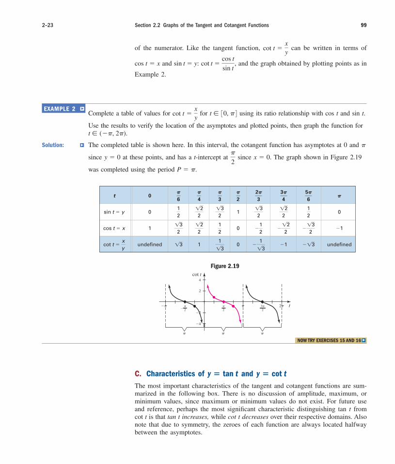
▼EXAMPLE 2Complete a table of values for for using its ratio relationship with cos t and sin t.
Use the results to verify the location of the asymptotes and plotted points, then graph the function for
Solution: The completed table is shown here. In this interval, the cotangent function has asymptotes at 0 and
since at these points, and has a t-intercept at since The graph shown in Figure 2.19
was completed using the period P � �.
x � 0.�
2y � 0
�
t � (��, 2�).
t � 30, � 4cot t �xy
NOW TRY EXERCISES 15 AND 16 ▼
cot t
t3�2
�2
��� 2��2
�4
�2
4
2
���
�
Figure 2.19
C. Characteristics of and
The most important characteristics of the tangent and cotangent functions are sum-marized in the following box. There is no discussion of amplitude, maximum, orminimum values, since maximum or minimum values do not exist. For future useand reference, perhaps the most significant characteristic distinguishing tan t fromcot t is that tan t increases, while cot t decreases over their respective domains. Alsonote that due to symmetry, the zeroes of each function are always located halfwaybetween the asymptotes.
y � cot ty � tan t
cob10054_ch02_77-158.qxd 10/12/06 4:49 PM Page 99 CONFIRMING PAGES

Since the tangent function is more common than the cotangent, many neededcalculations will first be done using the tangent function and its properties, then
reciprocated. For instance, to evaluate we reason that cot t is an odd
function, so Since cotangent is the reciprocal of tangent and
See Exercises 23 and 24.�cot a�
6b � �13.tan a�
6b �
113,
cot a��
6b � �cot a�
6b.
cot a��
6b
CHAPTER 2 Trigonometric Graphs and Models 2–24100
▼EXAMPLE 3Given what can you say about
and ?
Solution: Each of the arguments differs by a multiple of
and
Since the period of the tangent function is
all of these expressions have a value of 113
.P � �,
tan a�
6� �b.
tan a�5�
6b �tan a13�
6b � tan a�
6� 2�btan a�
6� �b,
tan a7�
6b ��:
tan a�5�
6b
tan a13�
6b,tan a7�
6b,tan a�
6b�
113,
NOW TRY EXERCISES 17 THROUGH 22 ▼
CHARACTERISTICS OF and
Unit Circle Unit CircleDefinition Domain Range Definition Domain Range
Period Behavior Symmetry Period Behavior Symmetry
increasing Odd decreasing Odd
cot1�t2 � �cot ttan1�t2 � �tan t
��
k � Zk � Z
y � 1�q, q 2t � k�cot t �xy
y � 1�q, q 2t �12k � 12�
2tan t �
yx
y � cot ty � tan ty � cot ty � tan t
D. Graphing y � A tan(Bt) and y � A cot(Bt)
The Coefficient A: Vertical Stretches and Compressions
For the tangent and cotangent functions, the role of coefficient A is best seen throughan analogy from basic algebra (the concept of amplitude is foreign to these func-tions). Consider the graph of (Figure 2.20), which you may recall has theappearance of a vertical propeller. Comparing the parent function with func-tions the graph is stretched vertically if (see Figure 2.21) and com-pressed if In the latter case the graph becomes very “flat” near thezeroes, as shown in Figure 2.22.
0 6 � A� 6 1.� A� 7 1y � Ax
3,y � x
3y � x
3
cob10054_ch02_77-158.qxd 10/12/06 4:49 PM Page 100 CONFIRMING PAGES

2–25 Section 2.2 Graphs of the Tangent and Cotangent Functions 101
x
y
x
y
x
y
Figure 2.20
y � x 3 y � 4x
3; A � 4 y � 14x
3; A � 14
Figure 2.21 Figure 2.22
While cubic functions are not asymptotic, they are a good illustration of A’s effecton the tangent and cotangent functions. Fractional values of A compress thegraph, flattening it out near its zeroes. Numerically, this is because a fractional part
of a small quantity is an even smaller quantity. For instance, compare with
To two decimal places, while so the
graph must be “nearer the t-axis” at this value.
1
4 tan a�
6b � 0.14,tan a�
6b � 0.57,
1
4 tan a�
6b.
tan a�
6b
( 0A 0 6 1)
▼EXAMPLE 4 Draw a “comparative sketch” of and on thesame axis and discuss similarities and differences. Use the inter-val ,
Solution: Both graphs will maintain their essential features (zeroes, asymp-totes, period increasing, and so on). However, the graph of
is vertically compressed, causing it to flatten out nearits zeroes and changing how the graph approaches its asymptotesin each interval.
y � 14 tan t
2� 4 .t � 3��
y � 14 tan ty � tan t
NOW TRY EXERCISES 25 THROUGH 28 ▼
y
t3�2
�2
��� 2��2
�4
�2
4
2
14
�
y � tan ty � tan t
The Coefficient B: The Period of Tangent and Cotangent
Like the other trig functions, the value of B has a material impact on the period ofthe function, and with the same effect. The graph of completes a cycle
twice as fast as versus while completes
a cycle one-half as fast versus This type of reasoning leads us to a period formula for tangent and cotangent,
namely, where B is the coefficient of the input variable.P ��
B,
P � �2.1P � 2�
y � cot a1
2 tbP � �b,aP �
�
2y � cot t
y � cot12t2W O R T H Y O F N OT E
It may be easier to interpret thephrase “twice as fast” as and “one-half as fast” as Ineach case, solving for P gives thecorrect interval for the period of thenew function.
12P � �.2P � �
cob10054_ch02_77-158.qxd 10/12/06 4:49 PM Page 101 CONFIRMING PAGES
CHAPTER 2 Trigonometric Graphs and Models 2–26102
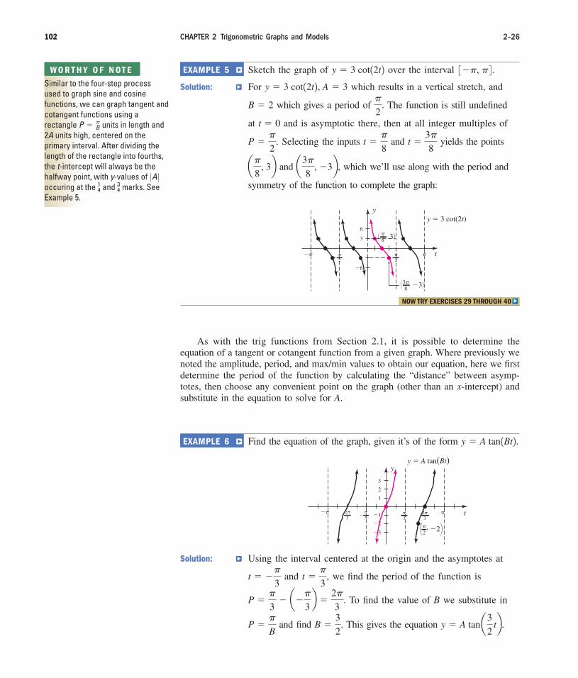
▼EXAMPLE 5 Sketch the graph of over the interval
Solution: For which results in a vertical stretch, and
which gives a period of The function is still undefined
at and is asymptotic there, then at all integer multiples of
Selecting the inputs and yields the points
and which we’ll use along with the period and
symmetry of the function to complete the graph:
a3�
8, �3b,a�
8, 3b
t �3�
8t �
�
8P �
�
2.
t � 0
�
2.B � 2
y � 3 cot12t2, A � 3
3��, � 4 .y � 3 cot12t2
NOW TRY EXERCISES 29 THROUGH 40 ▼
y � 3 cot(2t)
3�8� , �3�
�8� , 3�
y
t�2
��� �2
�6
6
3
�
As with the trig functions from Section 2.1, it is possible to determine theequation of a tangent or cotangent function from a given graph. Where previously wenoted the amplitude, period, and max/min values to obtain our equation, here we firstdetermine the period of the function by calculating the “distance” between asymp-totes, then choose any convenient point on the graph (other than an x-intercept) andsubstitute in the equation to solve for A.
▼EXAMPLE 6 Find the equation of the graph, given it’s of the form y � A tan1Bt2.y � A tan(Bt)
t�� 2�3
�3
��3
�2�3
�
y
�3
3
2
1
�1
�2�2� , �2�
Solution: Using the interval centered at the origin and the asymptotes at
and we find the period of the function is
To find the value of B we substitute in
and find This gives the equation y � A tan a3
2 tb.B �
3
2.P �
�
B
P ��
3� a��
3b �
2�
3.
t ��
3,t � �
�
3
W O R T H Y O F N OT E
Similar to the four-step processused to graph sine and cosinefunctions, we can graph tangent andcotangent functions using arectangle units in length and2A units high, centered on theprimary interval. After dividing thelength of the rectangle into fourths,the t-intercept will always be thehalfway point, with y-values of occuring at the and marks. SeeExample 5.
34
14
0A 0
P � �B
cob10054_ch02_77-158.qxd 10/12/06 4:49 PM Page 102 CONFIRMING PAGES

2–27 Section 2.2 Graphs of the Tangent and Cotangent Functions 103
To find A, we take the point given, and use with
to solve for A:
substitute for B
substitute for y and for t
multiply
solve for A
result
The equation of the graph is y � 2 tan A32 tB.� 2
A ��2
tan a3�
4b
�2 � A tan a3�
4b
�
2�2 �2 � A tan c a3
2b a�
2b d
32
y � A tan a3
2 tb
y � �2
t ��
2a�
2, �2b
NOW TRY EXERCISES 41 THROUGH 46 ▼
▼
E. Applications of Tangent and Cotangent Functions
We end this section with one example of how tangent and cotangent functions canbe applied. Numerous others can be found in the exercise set.
EXAMPLE 7 One evening, in port during a Semester at Sea, Marlon is debat-ing a project choice for his Precalculus class. Looking out hisporthole, he notices a revolvinglight turning at a constant speednear the corner of a long ware-house. The light throws its beamalong the length of the ware-house, then disappears into theair, and then returns time andtime again. Suddenly—Marlonhas his project. He notes thetime it takes the beam to traversethe warehouse wall is very closeto 4 sec, and in the morning he measures the wall’s length at127.26 m. His project? Modeling the distance of the beam from thecorner of the warehouse with a tangent function. Can you help?
Solution: The equation model will have the form whereis the distance (in meters) of the beam from the corner after
t sec. The distance along the wall is measured in positive valuesso we’re using only the period of the function, giving (the beam “disappears” at ) so Substitution in the
period formula gives and the equation D � A tan a�
8 tb.B �
�
8
P � 8.t � 4
12 P � 41
2
D 1t2 D 1t2 � A tan1Bt2,
cob10054_ch02_77-158.qxd 10/12/06 4:49 PM Page 103 CONFIRMING PAGES
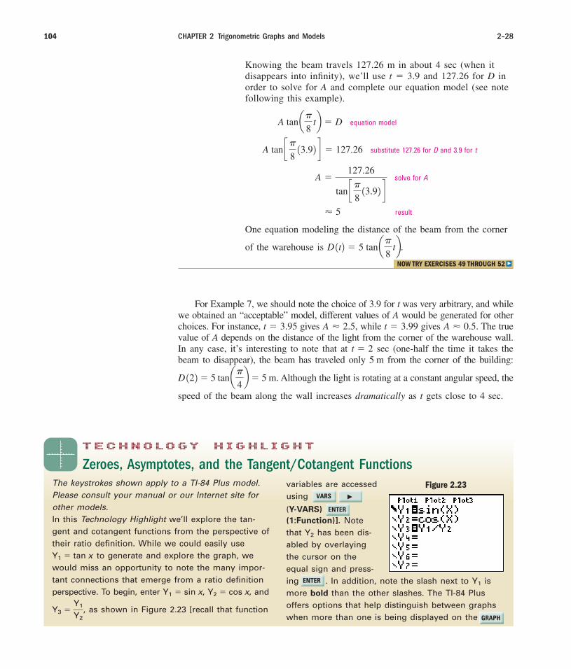
Knowing the beam travels 127.26 m in about 4 sec (when itdisappears into infinity), we’ll use t � 3.9 and 127.26 for D inorder to solve for A and complete our equation model (see notefollowing this example).
equation model
substitute 127.26 for D and 3.9 for t
solve for A
result
One equation modeling the distance of the beam from the corner
of the warehouse is D 1t2 � 5 tan a�
8 tb.
� 5
A �127.26
tan c�8
13.92 d
A tan c�8
13.92 d � 127.26
A tan a�
8 tb � D
CHAPTER 2 Trigonometric Graphs and Models 2–28104
NOW TRY EXERCISES 49 THROUGH 52 ▼
For Example 7, we should note the choice of 3.9 for t was very arbitrary, and whilewe obtained an “acceptable” model, different values of A would be generated for otherchoices. For instance, gives while gives The truevalue of A depends on the distance of the light from the corner of the warehouse wall.In any case, it’s interesting to note that at sec (one-half the time it takes thebeam to disappear), the beam has traveled only 5 m from the corner of the building:
Although the light is rotating at a constant angular speed, the
speed of the beam along the wall increases dramatically as t gets close to 4 sec.
D 122 � 5 tan a�
4b � 5 m.
t � 2
A � 0.5.t � 3.99A � 2.5,t � 3.95
TECHNOLOGY H IGHLIGHT
Zeroes, Asymptotes, and the Tangent/Cotangent FunctionsThe keystrokes shown apply to a TI-84 Plus model.
Please consult your manual or our Internet site for
other models.
In this Technology Highlight we’ll explore the tan-
gent and cotangent functions from the perspective of
their ratio definition. While we could easily use
to generate and explore the graph, we
would miss an opportunity to note the many impor-
tant connections that emerge from a ratio definition
perspective. To begin, enter and
as shown in Figure 2.23 [recall that functionY3 �Y1
Y2
,
Y2 � cos x,Y1 � sin x,
Y1 � tan x
variables are accessed
using
(Y-VARS)(1:Function)]. Note
that has been dis-
abled by overlaying
the cursor on the
equal sign and press-
ing . In addition, note the slash next to is
more bold than the other slashes. The TI-84 Plus
offers options that help distinguish between graphs
when more than one is being displayed on the
Y1
Y2
Figure 2.23
VARS �
ENTER
ENTER
GRAPH
cob10054_ch02_77-158.qxd 10/12/06 4:49 PM Page 104 CONFIRMING PAGES
2–29 Exercises 105
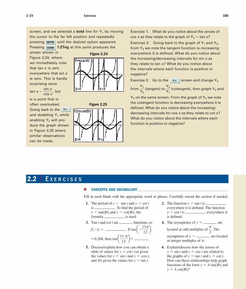
screen, and we selected a bold line for by moving
the cursor to the far left position and repeatedly
pressing until the desired option appeared.
Pressing 7:ZTrig at this point produces the
screen shown in
Figure 2.24, where
we immediately note
that is zero
everywhere that
is zero. This is hardly
surprising since
but
is a point that is
often overlooked.
Going back to the
and disabling while
enabling will pro-
duce the graph shown
in Figure 2.25 where
similar observations
can be made.
Y2
Y1
tan x �sin x
cos x ,
sin x
tan x
Y1 Exercise 1: What do you notice about the zeroes of
cos x as they relate to the graph of ?
Exercise 2: Going back to the graph of and
from we note the tangent function is increasing
everywhere it is defined. What do you notice about
the increasing/decreasing intervals for sin x as
they relate to tan x? What do you notice about
the intervals where each function is positive or
negative?
Exercise 3: Go to the m screen and change
from (tangent) to (cotangent), then graph and
on the same screen. From the graph of we note
the cotangent function is decreasing everywhere it is
defined. What do you notice about the increasing/
decreasing intervals for cos x as they relate to cot x?
What do you notice about the intervals where each
function is positive or negative?
Y3Y3
Y2
Y2
Y1
Y1
Y2
Y3
Y3
Y3,Y1
Y3 � tan x
Figure 2.25
Y�
2.2 E X E R C I S E S
CONCEPTS AND VOCABULARY
Fill in each blank with the appropriate word or phrase. Carefully reread the section if needed.
1. The period of and is . To find the period of
and theformula is used.
y � cot1Bt2,y � tan1Bt2y � cot ty � tan t 2. The function is
everywhere it is defined. The functionis everywhere it
is defined.y � cot t
y � tan t
3. and are functions, so
. If
then .tan a11 �
12b��0.268,
tan a�11�
12b ,f 1�t2 �
cot tTan t 4. The asymptotes of are
located at odd multiples of The
asymptotes of are locatedat integer multiples of .�
y �
�
2.
y �
5. Discuss/explain how you can obtain atable of values for (a) giventhe values for and and (b) given the values for y � tan t.
y � cos t,y � sin ty � cot t
6. Explain/discuss how the zeroes ofand are related to
the graphs of and How can these relationships help graphfunctions of the form and
?y � A cot1Bt2 y � A tan1Bt2y � cot t.y � tan t
y � cos ty � sin t
Figure 2.24
ZOOM
ENTER
Y�
cob10054_ch02_77-158.qxd 10/12/06 4:49 PM Page 105 CONFIRMING PAGES

CHAPTER 2 Trigonometric Graphs and Models 2–30106
9. Without reference to a text or calculator,attempt to name the decimal equivalent ofthe following values to one decimal place.
213
12
212
�
6
�
4
�
2
10. Without reference to a text or calculator,attempt to name the decimal equivalent ofthe following values to one decimal place.
113
13
213
3�
2�
�
3
DEVELOPING YOUR SKILLS
Use the values given for sin t and cos t to complete the tables.
t
0
0
tan t �y
x
�1
2�12
2�13
2�1cos t � x
�1�13
2�12
2�
1
2sin t � y
3�
24�
35�
47�
6�
0
0 1
tan t �y
x
13
2
12
2
1
2cos t � x
�1
2�12
2�13
2�1sin t � y
2�11�
67�
45�
33�
2
7. 8.
11. State the value of each expressionwithout the use of a calculator.
a. b.
c. d. tan a�
3bcot a3�
4b
cot a�
6btan a��
4b
12. State the value of each expression with-out the use of a calculator.
a. b.
c. d. cot a�5�
6btan a�
5�
4b
tan �cot a�
2b
13. State the value of each expression withoutthe use of a calculator, given terminates in the quadrant indicated.
a. in QIV
b. in QIII
c. in QIV
d. in QIItan t � �1, t
cot t � �113
, t
cot t � 13, t
tan t � �1, t
t � 30, 2�2 14. State the value of each expression withoutthe use of a calculator, given terminates in the quadrant indicated.
a. in QI
b. in QII
c. in QI
d. in QIIIcot t � 1, t
tan t �113
, t
tan t � �13, t
cot t � 1, t
t � 30, 2�2
Use the values given for sin t and cos t to complete the tables.
15. 16.
17. Given is a solution to
use the period of the function to namethree additional solutions. Check youranswer using a calculator.
tan t � 7.6,t �11�
2418. Given is a solution to
use the period of the function to namethree additional solutions. Check youranswer using a calculator.
cot t � 0.77,t �7�
24
t
0
0
cot t �x
y
�1
2�12
2�13
2�1cos t � x
�1�13
2�12
2�
1
2sin t � y
3�
24�
35�
47�
6�
0
0 1
cot t �x
y
13
2
12
2
1
2cos t � x
�1
2�12
2�13
2�1sin t � y
2�11�
67�
45�
33�
2
cob10054_ch02_096-113.qxd 11/22/06 9:40 AM Page 106

2–31 Exercises 107
Verify the value shown for t is a solution to the equation given, then use the period of thefunction to name all real roots. Check two of these roots on a calculator.
21. ; 22.
23. 24.
Graph each function over the interval indicated, noting the period, asymptotes, zeroes, andvalue of A. Include a comparative sketch of or as indicated.
25. 26.
27. 28.
Graph each function over the interval indicated, noting the period, asymptotes, zeroes, andvalue of A.
29. 30.
31. 32.
33. 34.
35. 36.
37. 38.
39. 40.
Find the equation of each graph, given it is of the form
41.
42. y
t�6
�6
�3
�3
�2
�2
�2
�1
2
1
�12
12� , �� �
y
t3�2
3�2
�2
� 2��2� �� �2
�9
9
��
�2� , 3�
y � A tan1Bt2.3�4, 44p 1t2� 1
2 cot a�
4 tb;3�1, 1 4f 1t2 � 2 cot1�t2;3�2, 2 4y � 4 tan a�
2 tb;c�1
2,
1
2dy � 3 tan12�t2;
c��
2,
�
2dy �
1
2 cot12t2;3�3�, 3�4y � 5 cot a1
3 tb;
3�2�, 2�4y � 4 tan a12
tb;c��
4,
�
4dy � 2 tan14t2;
3�2�, 2� 4y � cot a1
2 tb;c��
4,
�
4dy � cot14t2;
3�4�, 4� 4y � tan a1
4 tb;c��
2,
�
2dy � tan 12t2;
3�2�, 2� 4r 1t2 �1
4 cot t;3�2�, 2� 4h 1t2 � 3 cot t;
3�2�, 2� 4g1t2 �1
2 tan t;3�2�, 2� 4f 1t2 � 2 tan t;
y � cot ty � tan t
cot t � 2 � 13.t �5�
12;cot t � 2 � 13t �
�
12;
tan t � �0.1989t � ��
16;tan t � 0.3249t �
�
10
19. Given is a solution touse the period of the func-
tion to name three additional solutions.Check your answers using a calculator.
cot t � 0.07,t � 1.5 20. Given is a solution to
use the period of the functionto name three additional solutions.Check your answers using a calculator.
tan t � 3,t � 1.25
cob10054_ch02_77-158.qxd 10/12/06 4:49 PM Page 107 CONFIRMING PAGES

CHAPTER 2 Trigonometric Graphs and Models 2–32108
Find the equation of each graph, given it is of the form
43. 44. 19� , √3 �
16
12
13
16�
13
�12
�
y
t
�3
3
14� , 2√3 �y
t
�3
3
32�1�2�3 1
y � A cot1Bt2.
45. Given that and are
solutions to use a graph-ing calculator to find two additionalsolutions in .30, 2� 4
cot13t2 � tan t,
t � �3�
8t � �
�
846. Given is a solution to
use a graphing calculator tofind two additional solutions in 3�1, 1 4 .cot 1�t2, tan12�t2 �t � 1
6
WORKING WITH FORMULAS
47. Position of an image reflected from a spherical lens:
The equation shown is used to help locate theposition of an image reflected by a spherical mirror,where s is the distance of the object from the lensalong a horizontal axis, is the angle of elevationfrom this axis, h is the altitude of the right triangleindicated, and k is distance from the lens to the footof altitude h. Find the distance k given mm,
and that the object is 24 mm from the lens.
48. The height of an object calculated from a distance:
The height h of a tall structure can be computed using twoangles of elevation measured some distance apart along astraight line with the object. This height is given by theformula shown, where d is the distance between the twopoints from which angles u and v were measured. Find theheight h of a building if and ft.
APPLICATIONS
Tangent function data models: Model the data in Exercises 49 and 50 using the functiony A tan(Bx). State the period of the function, the location of the asymptotes, the valueof A, and name the point (x, y) used to calculate A (answers may vary). Use your equationmodel to evaluate the function at and What observations can you make?Also see Exercise 58.
49. 50.
x � 2.x � �2
�
d � 100v � 65�,u � 40�,
h �d
cot u � cot v
� ��
24,
h � 3
�
tan � �h
s � k
Lens
PObject
PReflected
image
k
s
h�
d x � d
h
u v
Input Output Input Output
1 1.4
2 3
3 5.2
4 9.7
5 20
1 6
0 0
q�1.4
�3�2
�5.2�3
�9.7�4
�20�5
�q�6
Input Output Input Output
0.5 6.4
1 13.7
1.5 23.7
2 44.3
2.5 91.3
3
0 0
q�6.4�0.5
�13.7�1
�23.7�1.5
�44.3�2
�91.3�2.5
�q�3
cob10054_ch02_77-158.qxd 10/12/06 4:49 PM Page 108 CONFIRMING PAGES

2–33 Exercises 109
51. As part of a lab setup, a laser pen is made to swivel on alarge protractor as illustrated in the figure. For their labproject, students are asked to take the instrument to oneend of a long hallway and measure the distance of theprojected beam relative to the angle the pen is beingheld, and collect the data in a table. Use the data to find afunction of the form State the period ofthe function, the location of the asymptotes, the value ofA, and name the point ( , y) you used to calculate A(answers may vary). Based on the result, can youapproximate the length of the laser pen? Note that in
degrees, the period formula for tangent is
52. Use the equation model obtained in Exercise 51 to comparethe values given by the equation with the actual data. As apercentage, what was the largest deviation between the two?
53. Circumscribed polygons: The perimeter of a regular polygon circumscribed about a
circle of radius r is given by where n is the number of sides
and r is the radius of the circle. Given cm, (a) What is the perimeter of the circle?(b) What is the perimeter of the polygon when ? Why? (c) Calculate the perimeter ofthe polygon for 20, 30, and 100. What do you notice?
54. Circumscribed polygons: The area of a regular polygon circumscribed about a circle of
radius r is given by where n is the number of sides and r is the
radius of the circle. Given cm,
a. What is the area of the circle?
b. What is the area of the polygon when ? Why?
c. Calculate the area of the polygon for 20, 30, and 100. What do you notice?
Coefficients of friction: Pulling someone on a sledis much easier during the winter than in the sum-mer, due to a phenomenon known as the coefficientof friction. The friction between the sled’s skidsand the snow is much lower than the frictionbetween the skids and the dry ground or pavement.Basically, the coefficient of friction is defined by therelationship where is the angle atwhich a block composed of one material will slidedown an inclined plane made of another material, with a constant velocity. Coefficients offriction have been established experimentally for many materials and a short list is shown here.
55. Graph the function with in degrees over the interval and use thegraph to estimate solutions to the following. Confirm or contradict your estimates using acalculator.
a. A block of copper is placed on a sheet of steel, which is slowly inclined. Is the blockof copper moving when the angle of inclination is ? At what angle of inclinationwill the copper block be moving with a constant velocity down the incline?
b. A block of copper is placed on a sheet of cast-iron. As the cast-iron sheet is slowlyinclined, the copper block begins sliding at a constant velocity when the angle of inclina-tion is approximately What is the coefficient of friction for copper on cast-iron?
c. Why do you suppose coefficients of friction greater than are extremelyrare? Give an example of two materials that likely have a high -value.�
� � 2.5
46.5�.
30�
30�, 60� 4�� � tan �
�� � tan �,
n � 10,
n � 4
r � 10
1n � 32A � nr2tan a�
nb,
n � 10,n � 4
r � 10
1n � 3 2tan a�nb,P � 2nr
P �180°
B.
�
y � A tan1B�2.L
aser
Lig
ht
Distance(degrees) (cm)
0 0
10 2.1
20 4.4
30 6.9
40 10.1
50 14.3
60 20.8
70 33.0
80 68.1
89 687.5
�
r
Exercise 53
Exercise 51
Material Coefficient
steel on steel 0.74
copper on glass 0.53
glass on glass 0.94
copper on steel 0.68
wood on wood 0.5
cob10054_ch02_77-158.qxd 10/12/06 4:50 PM Page 109 CONFIRMING PAGES

CHAPTER 2 Trigonometric Graphs and Models 2–34110
56. Graph the function with in radians over the interval and use the
graph to estimate solutions to the following. Confirm or contradict your estimates using acalculator.
a. A block of glass is placed on a sheet of glass, which is slowly inclined. Is the block of
glass moving when the angle of inclination is ? What is the smallest angle of
inclination for which the glass block will be moving with a constant velocity downthe incline (rounded to four decimal places)?
b. A block of Teflon is placed on a sheet of steel. As the steel sheet is slowly inclined,the Teflon block begins sliding at a constant velocity when the angle of inclination isapproximately 0.04. What is the coefficient of friction for Teflon on steel?
c. Why do you suppose coefficients of friction less than are extremely rarefor two solid materials? Give an example of two materials that likely have a very low
value.
57. Tangent lines: The actual definition of the word tangent comesfrom the Latin tangere, meaning “to touch.” In mathematics, atangent line touches the graph of a circle at only one point andfunction values for are obtained from the length of theline segment tangent to a unit circle.
a. What is the length of the line segment when ?
b. If the line segment is 16.35 units long, what is the valueof ?
c. Can the line segment ever be greater than 100 units long?Why or why not?
d. How does your answer to (c) relate to the asymptotic behavior of the graph?
WRITING, RESEARCH, AND DECISION MAKING
58. Rework Exercises 49 and 50, obtaining a new equation for the data using a differentordered pair to compute the value of A. What do you notice? Try yet another ordered pairand calculate A once again for another equation . Complete a table of values using thegiven inputs, with the outputs of the three equations generated (original, and Does any one equation seem to model the data better than the others? Are all of theequation models “acceptable”? Please comment.
59. The golden ratio has long been thought to be the most pleasing ratio in art and
architecture. It is commonly believed that many forms of ancient architecture wereconstructed using this ratio as a guide. The ratio actually turns up in some surprisingplaces, far removed from its original inception as a line segment cut in “mean andextreme” ratio. Do some research on the golden ratio and some of the equations that havebeen used to produce it. Given , try to find a connection between
and
EXTENDING THE CONCEPT
60. Regarding Example 7, we can use the standard distance/rate/time formula tocompute the average velocity of the beam of light along the wall in any interval of time:
For example, using the average velocity in the interval 30, 2 4D 1t2 � 5 tan a�
8 tb,R �
D
T.
D � RT
y � sin x.y � cos x, y � tan x,x � 0.6662394325
�1 � 15
2
Y22.Y1,Y2
�
� � 80�
tan �
�
� � 0.04
�
4
c0, 5�
12d�� � tan �
1
tan �
�
cob10054_ch02_77-158.qxd 10/12/06 4:50 PM Page 110 CONFIRMING PAGES

2–35 Exercises 111
is Calculate the average velocity of the beam in the time
intervals , and sec. What do you notice? How would the averagevelocity of the beam in the interval sec compare?
61. Determine the slope of the line drawn through the parabola (called a secant line) inFigure I. Use the same method (any two points on the line) to calculate the slope of theline drawn tangent to the parabola in Figure II. Compare your calculations to the tangentof the angles and that each line makes with the x-axis. What can you conclude? Writea formula for the point/slope equation of a line using instead of m.tan �
��
33.9, 3.99 433.5, 3.8 433, 3.5 4 ,32, 3 42.5 m/sec.
D122 � D1022 � 0
�
5 10
5
10
�
y
x 5 10
5
10
x
y
�
Exercise 62 Exercise 63
Figure I Figure II
2 ft
4 ft
�
r
MAINTAINING YOUR SKILLS
62. (1.2) A tent rope is 4 ft long and attached to the tent wall 2 ft above the ground. How farfrom the tent is the stake holding the rope?
63. (1.1) A lune is a section of surface area on a sphere, which is subtended by an angle atthe circumference. For in radians, the surface area of a lune is where r is theradius of the sphere. Find the area of a lune on the surface of the Earth which is subtendedby an angle of Assume the radius of the Earth is 6373 km.
64. (1.4) Use a reference arc to determine the value of
65. (1.4) State the points on the unit circle that correspond to and
What is the value of ? Why?
66. (1.3) Given find another angle in that satisfieswithout using a calculator.
67. (2.1) At what value(s) of t does the horizontal line intersect the graph ofy � �3 sin t?
y � 3
sin � � �0.5330�, 360�2�sin 212° � �0.53,
tan a�
2b2�.
3�
2,
3�
4,�,
�
2,
�
4,t � 0,
cos a29�
6b.
15�.
A � 2r 2�,�
�
I. II.
cob10054_ch02_77-158.qxd 10/12/06 4:50 PM Page 111 CONFIRMING PAGES
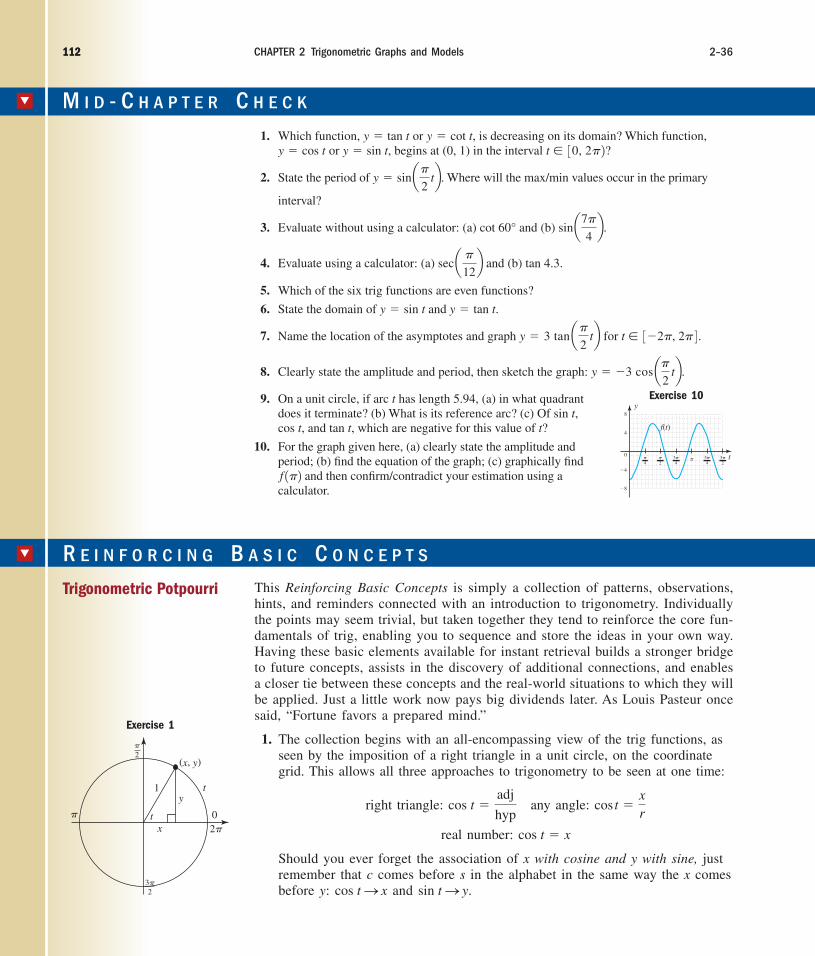
CHAPTER 2 Trigonometric Graphs and Models 2–36112
▼ R E I N F O R C I N G B A S I C C O N C E P T S
Trigonometric Potpourri This Reinforcing Basic Concepts is simply a collection of patterns, observations,hints, and reminders connected with an introduction to trigonometry. Individuallythe points may seem trivial, but taken together they tend to reinforce the core fun-damentals of trig, enabling you to sequence and store the ideas in your own way.Having these basic elements available for instant retrieval builds a stronger bridgeto future concepts, assists in the discovery of additional connections, and enablesa closer tie between these concepts and the real-world situations to which they willbe applied. Just a little work now pays big dividends later. As Louis Pasteur oncesaid, “Fortune favors a prepared mind.”
1. The collection begins with an all-encompassing view of the trig functions, asseen by the imposition of a right triangle in a unit circle, on the coordinategrid. This allows all three approaches to trigonometry to be seen at one time:
right triangle: any angle:
real number:
Should you ever forget the association of x with cosine and y with sine, justremember that c comes before s in the alphabet in the same way the x comesbefore y: and sin t S y.cos t S x
cos t � x
cos t �xr
cos t �adj
hyp
(x, y)
t
ty
x�
1
0
3�2
2�
�2
Exercise 1
112
1. Which function, or is decreasing on its domain? Which function,or begins at (0, 1) in the interval
2. State the period of Where will the max/min values occur in the primary
interval?
3. Evaluate without using a calculator: (a) and (b) .
4. Evaluate using a calculator: (a) and (b)
5. Which of the six trig functions are even functions?
6. State the domain of
7. Name the location of the asymptotes and graph for
8. Clearly state the amplitude and period, then sketch the graph:
9. On a unit circle, if arc t has length 5.94, (a) in what quadrantdoes it terminate? (b) What is its reference arc? (c) Of sin t,cos t, and tan t, which are negative for this value of t?
10. For the graph given here, (a) clearly state the amplitude andperiod; (b) find the equation of the graph; (c) graphically find
and then confirm/contradict your estimation using acalculator.f 1�2
y � �3 cos a�2
tb.t � 3�2�, 2� 4 .y � 3 tan a�
2 tb
y � sin t and y � tan t.
tan 4.3.sec a �
12b
sin a7�
4bcot 60°
y � sin a�
2 tb.
t � 30, 2� 2?y � sin t,y � cos ty � cot t,y � tan t
�8
�4
0
8
4
y
t
f(t)
�4
�2
3�4
5�4
3�2
�
Exercise 10
M I D - C H A P T E R C H E C K▼
cob10054_ch02_77-158.qxd 10/12/06 4:50 PM Page 112 CONFIRMING PAGES

2-37 Reinforcing Basic Concepts 113
2. Know the standard angles and the standard values. As mentioned earlier, theyare used repeatedly throughout higher mathematics to introduce new conceptsand skills without the clutter and distraction of large decimal values. It isinteresting to note the standard values (from QI) can always be recreated usingthe pattern of fourths. Simply write the fractions with integer numerators from
through , and take their square root:
3. There are many decimal equivalents in elementary mathematics that contributeto concept building. In the same way you recognize the decimal values of
and others, it helps tremendously to recognize or “know” decimal equiva-lents for values that are commonly used in a study of trig. They help toidentify the quadrant of an arc/angle’s terminal side when t is expressed inradians, they assist in graphing and estimation skills, and are used extensivelythroughout this text and in other areas of mathematics. In terms of these are
and In terms of radicals they are , , and
Knowing leads directly to and while adding the
decimal values for and gives Further, since
and since
4. To specifically remember what standard value is associated with a standardangle or arc, recall that
a. If t is a quadrantal arc/angle, it’s easiest to use the coordinates (x, y) of apoint on a unit circle.
b. If t is any odd multiple of sin t and cos t must be or with
the choice depending on the quadrant of the terminal side. The values of the other functions can be found using these.
c. If t is a multiple of (excluding the quadrantal angles), the value for sine
and cosine must be either or depending on the quadrant of the
terminal side. If there’s any hesitationabout which value applies to sine and which to cosine, mental imagery can once
again help. Since
we simply apply the larger value to the
larger arc/angle. Note that for the triangle
drawn in QI angle at vertex ,
y is obviously longer than x, meaning the
ba�
3� 60°
13
2� 0.87 7
1
2� 0.5,
�13
2,�
1
2
�
6
12
2,�
12
2
�
4,
13
2� 0.87.13 � 1.73,
12 � 1.41, 12
2� 0.7,
3�
2� 4.71.
�
2�
2� � 6.28,�
2� 1.57� � 3.14
13
2.13
12
2,122�.
3�
2,�,
�
2,
�
34,
12,1
4,
A4
4� 1A3
4�13
2A2
4�12
2A1
4�
1
2A0
4� 0
44
04
(x, y)
(x, y)y
y
xx�
y
x
1
0
3�2
2�
�2
cob10054_ch02_77-158.qxd 10/12/06 4:50 PM Page 113 CONFIRMING PAGES

CHAPTER 2 Trigonometric Graphs and Models 2–38114
2.3 Transformations and Applications of Trigonometric GraphsINTRODUCTION
From your algebra experience, you may remember beginning with a study of lineargraphs, then moving on to quadratic graphs and their characteristics. By combiningand extending the knowledge you gained, you were able to investigate and under-stand a variety of polynomial graphs—along with some powerful applications. Astudy of trigonometry follows a similar pattern, and by “combining and extending”our understanding of the basic trig graphs, we’ll look at some powerful applicationsin this section.
LEARNING OBJECTIVES
In Section 2.3 you will learn how to:
A. Apply vertical translations incontext
B. Apply horizontal translationsin context
C. Solve applications involvingharmonic motion
P O I N T O F I N T E R E S T
In some coastal areas, tidal motion is simple, predictable, and under perfect con-
ditions can be approximated using a single sine function. In other areas, how-
ever, a combination of factors make the motion much more complex, although
still predictable. The mathematical model for these tides requires more than a
single trig function, a concept known as the addition of ordinates. Similar
concepts also apply in areas such as sound waves and musical tones.
▼
association must be and For the triangle in QII
whose reference angle is , x is longer than y, meaning
the association must be and
5. Although they are often neglected or treated lightly in a study of trig, thesecant, cosecant, and cotangent functions play an integral role in moreadvanced mathematics classes. Be sure you’re familiar with their reciprocalrelationship to the more common cosine, sine, and tangent functions:
6. Finally, the need to be very familiar with the basic graphs of the trig functionswould be hard to overstate. As with transformations of the toolbox functions(from algebra), transformations of the basic trig graphs are a huge help to theunderstanding and solution of trig equations and inequalities, as well as totheir application in the context of real-world phenomena.
tan 60° � 13 S cot 60° �113
tan t � 1;cot ttan t �1
cot t,cot t �
1
tan t,
sin a2�
3b �13
2S csc a2�
3b�
213sin t � 1;csc tsin t �
1
csc t,csc t �
1
sin t,
sec a2�
3b� �2Scos a2�
3b � �
1
2cos t � 1;sec tcos t �
1
sec t ,sec t �
1
cos t ,
sin t �1
2.cos t � �
13
2
b30°a5�
6� 150°
cos t �1
2.sin t �
13
2
114
cob10054_ch02_77-158.qxd 10/12/06 5:04 PM Page 114 CONFIRMING PAGES

2–39 Section 2.3 Transformations and Applications of Trigonometric Graphs 115
▼
A. Vertical Translations: y � A sin(Bt) � D
On any given day, outdoor temperatures tend to follow a sinusoidal pattern, or apattern that can be modeled by a sine function. As the sun rises, the morning tem-perature begins to warm and rise until reaching its high in the late afternoon, thenbegins to cool during the early evening and nighttime hours until falling to its night-time low just prior to sunrise. Next morning, the cycle begins again. In the northernlatitudes where the winters are very cold, it’s not unreasonable to assume an aver-age daily temperature of and a temperature graph in degrees Celsius thatlooks like the one in Figure 2.26. For the moment, we’ll assume that corre-sponds to 12:00 noon.
t � 0132°F2,0°C
6 12 18 24 t
�C
�15�
15�
Figure 2.26
EXAMPLE 1 Use the graph in Figure 2.26 to: (a) state the amplitude and periodof the function, (b) estimate the temperature at 9:00 P.M., and(c) estimate the number of hours the temperature is below
Solution: a. By inspection we see the amplitude of the graph is since this is the maximum displacement from the averagevalue. As the context and graph indicate, the period is 24 hr.
b. Since 9:00 P.M. corresponds to we read along the t-axisto 9, then move up to the graph to approximate the relatedtemperature value on the axis (see figure). It appears thetemperature will be close to
c. In part (b) we’re given the time and asked for a temperature.Here we’re given a temperature and asked for a time. Beginon the axis at move horizontally until you intersectthe graph, then move upward to the t-axis. The temperature isbelow for about 5 hr (from to t � 20.5.2t � 15.512°C
�12°,°C
11°C.°C
t � 9,
�A� � 15,
�12°C.
NOW TRY EXERCISES 7 THROUGH 10 ▼
If you live in a more temperate area, the daily temperatures still follow a sinusoidalpattern, but the average temperature could be much higher. This is an example of a ver-tical shift, and is the role D plays in the equation All other aspectsof a graph remain the same; it is simply shifted D units up if and D units down
if As in Section 2.1, for maximum value M and minimum value m,
gives the amplitude A of a sine curve, while gives the average value D.
From Example 1 we have and 15 � 1�152
2� 15✓.
15 � 1�1522
� 0
M � m
2
M � m
2D 6 0.
D 7 0y � A sin1Bt2 � D.
6 12 18
�15�
15�
t
�C
�15�
15�
(b)
(c)24
cob10054_ch02_77-158.qxd 10/12/06 5:04 PM Page 115 CONFIRMING PAGES
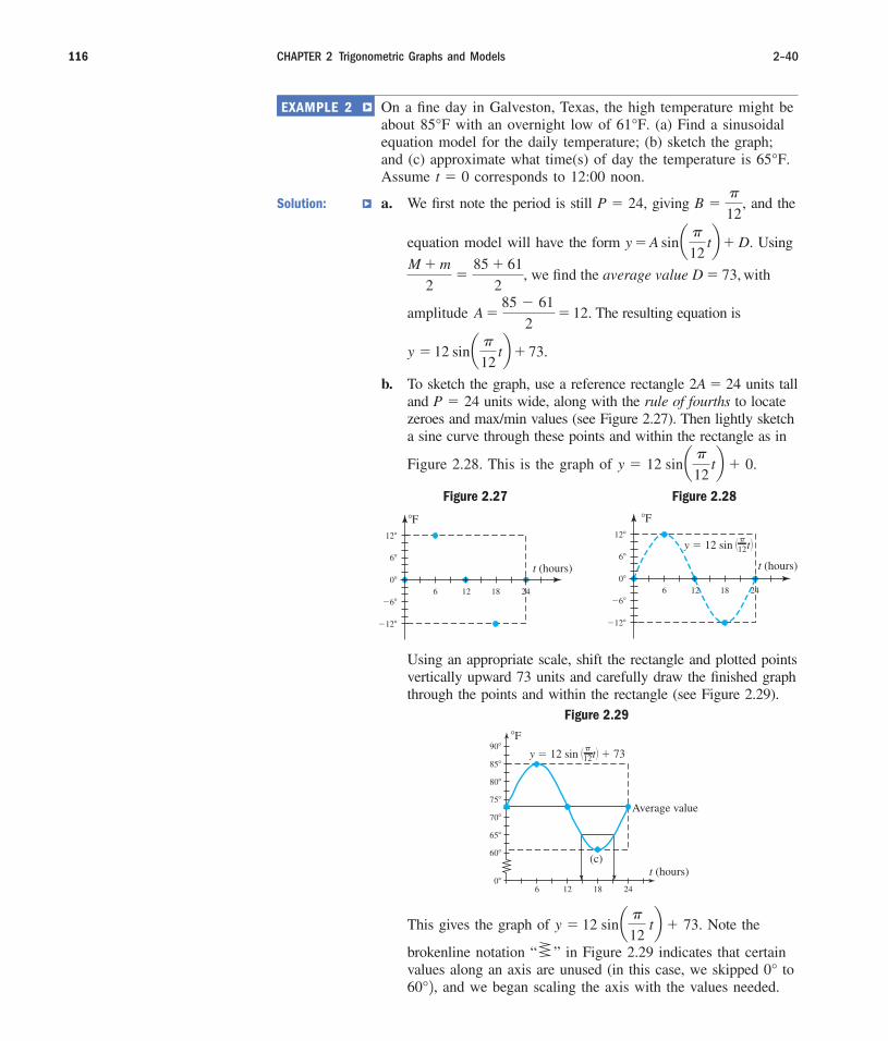
▼EXAMPLE 2 On a fine day in Galveston, Texas, the high temperature might beabout with an overnight low of (a) Find a sinusoidalequation model for the daily temperature; (b) sketch the graph;and (c) approximate what time(s) of day the temperature is Assume corresponds to 12:00 noon.
Solution: a. We first note the period is still giving and the
equation model will have the form Using
we find the average value with
amplitude The resulting equation is
b. To sketch the graph, use a reference rectangle units talland units wide, along with the rule of fourths to locatezeroes and max/min values (see Figure 2.27). Then lightly sketcha sine curve through these points and within the rectangle as in
Figure 2.28. This is the graph of y � 12 sin a �
12 tb � 0.
P � 242A � 24
y � 12 sin a �
12 tb� 73.
A �85 � 61
2� 12.
D � 73,M � m
2�
85 � 61
2,
y � A sin a �
12 tb� D.
B ��
12,P � 24,
t � 065°F.
61°F.85°F
CHAPTER 2 Trigonometric Graphs and Models 2–40116
Figure 2.27
Figure 2.29
Figure 2.28
6 12 18 24
t (hours)
�F
�12�
�6�
12�
6�
0�6 12 18 24
t (hours)
�F
�12�
�6�
12�
6�
0�
y � 12 sin � t��12
Using an appropriate scale, shift the rectangle and plotted pointsvertically upward 73 units and carefully draw the finished graphthrough the points and within the rectangle (see Figure 2.29).
y � 12 sin � t� � 73�12
12 18 2460�
t (hours)
Average value
�F
65�
75�
85�
60�
70�
80�
90�
(c)
This gives the graph of Note the
brokenline notation “ ” in Figure 2.29 indicates that certainvalues along an axis are unused (in this case, we skipped to
and we began scaling the axis with the values needed.60°2, 0°
y � 12 sin a �
12 tb � 73.
cob10054_ch02_77-158.qxd 10/12/06 5:04 PM Page 116 CONFIRMING PAGES
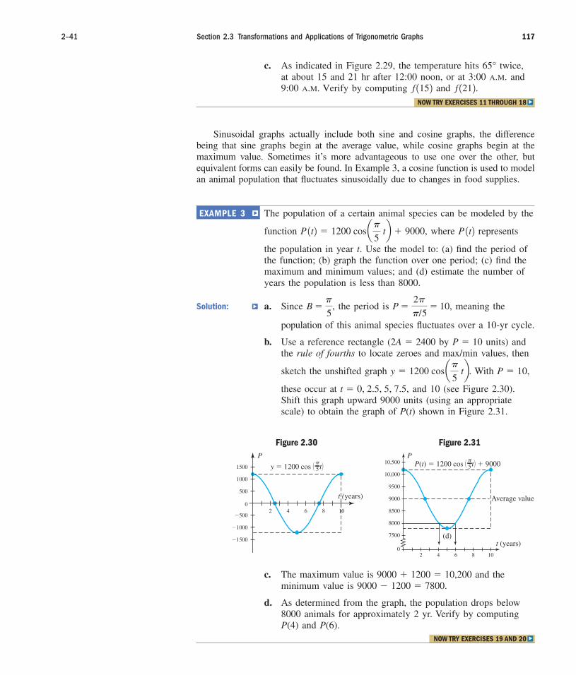
2–41 Section 2.3 Transformations and Applications of Trigonometric Graphs 117
▼
c. As indicated in Figure 2.29, the temperature hits twice,at about 15 and 21 hr after 12:00 noon, or at 3:00 A.M. and9:00 A.M. Verify by computing and .f 1212f 1152
65°
NOW TRY EXERCISES 11 THROUGH 18 ▼
Sinusoidal graphs actually include both sine and cosine graphs, the differencebeing that sine graphs begin at the average value, while cosine graphs begin at themaximum value. Sometimes it’s more advantageous to use one over the other, butequivalent forms can easily be found. In Example 3, a cosine function is used to modelan animal population that fluctuates sinusoidally due to changes in food supplies.
EXAMPLE 3 The population of a certain animal species can be modeled by the
function where represents
the population in year t. Use the model to: (a) find the period ofthe function; (b) graph the function over one period; (c) find themaximum and minimum values; and (d) estimate the number ofyears the population is less than 8000.
Solution: a. Since the period is meaning the
population of this animal species fluctuates over a 10-yr cycle.
b. Use a reference rectangle ( by units) andthe rule of fourths to locate zeroes and max/min values, then
sketch the unshifted graph With
these occur at and 10 (see Figure 2.30).Shift this graph upward 9000 units (using an appropriatescale) to obtain the graph of P(t) shown in Figure 2.31.
t � 0, 2.5, 5, 7.5,
P � 10,y � 1200 cos a�
5 tb.
P � 102A � 2400
P �2�
�/5� 10,B �
�
5,
P 1t2P 1t2 � 1200 cos a�
5 tb � 9000,
2 4 6 8 10
�1500
1500
1000
500
0
�1000
�500
y � 1200 cos � t��5
P
t (years)
P(t) � 1200 cos � t� � 9000�5
102 4 6 80
t (years)
Average value
P10,500
10,000
9500
9000
8000
8500
7500 (d)
Figure 2.30 Figure 2.31
c. The maximum value is and theminimum value is
d. As determined from the graph, the population drops below8000 animals for approximately 2 yr. Verify by computingP(4) and P(6).
9000 � 1200 � 7800.9000 � 1200 � 10,200
NOW TRY EXERCISES 19 AND 20 ▼
cob10054_ch02_77-158.qxd 10/12/06 5:04 PM Page 117 CONFIRMING PAGES

▼
B. Horizontal Translations: y � A sin(Bt � C) � D
In some cases, scientists would rather “benchmark” their study of sinusoidal phenom-enon by placing the average value at instead of a maximum value (as in Exam-ple 3), or by placing the maximum or minimum value at instead of the averagevalue (as in Example 1). Rather than make additional studies or recompute using avail-able data, we can simply shift these graphs using a horizontal translation. To help under-stand how, consider the graph of . The graph is a parabola, concave up, with avertex at the origin. Comparing this function with and we note is simply the parent graph shifted 3 units right, and is the parent graphshifted 3 units left (“opposite the sign”). See Figures 2.32 through 2.34.
y2y1
y2 � 1x � 322,y1 � 1x � 322y � x2
t � 0t � 0
CHAPTER 2 Trigonometric Graphs and Models 2–42118
x
y
x
y
3 x
y
�3
Figure 2.32
y � x2
Figure 2.33
y1 � 1x � 322Figure 2.34
y2 � 1x � 322
While quadratic functions have no maximum value if these graphs area good reminder of how a basic graph can be horizontally shifted. We simply replacethe independent variable x with or t with where h is the desiredshift and the sign is chosen depending on the direction of the shift.
1t � h2,1x � h2A � 0,
EXAMPLE 4 Use a horizontal translation to shift the graph from Example 3 sothat the average population value begins at Verify the resulton a graphing calculator, then find a sine function that gives thesame graph as the shifted cosine function.
Solution: For from Example 3, the average
value first occurs at For theaverage value to occur at wecan shift the graph to the right 2.5 units.Replacing t with gives
A graphing calculator shows thedesired result is obtained (see figure),and it appears to be a sine function with the same amplitude
and period. The equation is y � 1200 sin a�
5 tb � 9000.
P 1t2 � 1200 cos c�5
1t � 2.52 d � 9000.
1t � 2.52t � 0,
t � 2.5.
P 1t2 � 1200 cos a�
5 tb� 9000
t � 0.
NOW TRY EXERCISES 21 AND 22 ▼
cob10054_ch02_77-158.qxd 10/17/06 2:06 PM Page 118CONFIRMING PAGES
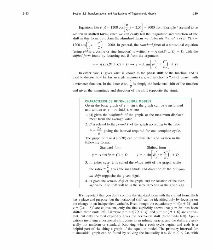
2–43 Section 2.3 Transformations and Applications of Trigonometric Graphs 119
Equations like from Example 4 are said to be
written in shifted form, since we can easily tell the magnitude and direction of theshift in this form. To obtain the standard form we distribute the value of B:
In general, the standard form of a sinusoidal equation
(using either a cosine or sine function) is written with theshifted form found by factoring out B from the argument:
In either case, C gives what is known as the phase shift of the function, and isused to discuss how far (as an angle measure) a given function is “out of phase” with
a reference function. In the latter case, is simply the horizontal shift of the function
and gives the magnitude and direction of the shift (opposite the sign).
C
B
y � A sin1Bt � C2 � D S y � A sin cB at �C
Bb d � D
y � A sin1Bt � C2 � D,
1200 cos a�
5 t �
�
2b � 9000.
P 1t2 �
P 1t2 � 1200 cos c�5
1t � 2.52 d � 9000
It’s important that you don’t confuse the standard form with the shifted form. Eachhas a place and purpose, but the horizontal shift can be identified only by focusing onthe change in an independent variable. Even though the equations and
are equivalent, only the first explicitly shows that has beenshifted three units left. Likewise and are equiva-lent, but only the first explicitly gives the horizontal shift (three units left). Appli-cations involving a horizontal shift come in an infinite variety, and the shifts are gen-erally not uniform or standard. Knowing where each cycle begins and ends is ahelpful part of sketching a graph of the equation model. The primary interval fora sinusoidal graph can be found by solving the inequality with0 � Bt � C 6 2�,
y � sin 12t � 62y � sin 321t � 32 4 y � 2x 2y � 12x � 622 y � 41x � 322
CHARACTERISTICS OF SINUSOIDAL MODELS
Given the basic graph of the graph can be transformedand written as where
1. gives the amplitude of the graph, or the maximum displace-ment from the average value.
2. B is related to the period P of the graph according to the ratio
giving the interval required for one complete cycle.
The graph of can be translated and written in thefollowing forms:
Standard form Shifted form
3. In either case, C is called the phase shift of the graph, while
the ratio gives the magnitude and direction of the horizon-
tal shift (opposite the given sign).
4. D gives the vertical shift of the graph, and the location of the aver-age value. The shift will be in the same direction as the given sign.
�
C
B
y � A sin cB at �C
Bb d � Dy � A sin1Bt � C2 � D
y � A sin1Bt2P �
2�
B,
�A�y � A sin1Bt2,y � sin t,
cob10054_ch02_77-158.qxd 10/12/06 5:04 PM Page 119 CONFIRMING PAGES

▼
the reference rectangle and rule of fourths giving the zeroes, max/min values, and asketch of the graph in this interval. The graph can then be extended as needed ineither direction, then shifted vertically D units.
CHAPTER 2 Trigonometric Graphs and Models 2–44120
EXAMPLE 5 For each function, identify the amplitude, period, horizontal shift,vertical shift (average value), and endpoints of the primary interval.
a.
b.
Solution: a. The equation shows amplitude with an average valueof This indicates the maximum value will be
with a minimum of
Since the period is With
the argument in factored form, we note the horizontal shift is6 units to the right (6 units opposite the sign). For the endpoints
of the primary interval we solve giving
b. The equation shows amplitude with an average valueof The maximum value will be
with a minimum of With the
period is To find the horizontal shift, we factor
out from the argument to place the equation in shifted
form: The horizontal shift is 3 units
left (3 units opposite the sign). For the endpoints of the primary
interval we solve which gives �3 � t 6 5.0 ��
4 1t � 32 6 2�,
a�
4 t �
3�
4b �
�
4 1t � 32.
�
4
P �2�
�/4� 8.
B ��
4,y � 2.51�12 � 6 � 3.5.
y � 2.5112 � 6 � 8.5,D � 6.�A� � 2.5,
6 � t 6 22.
0 ��
8 1t � 62 6 2�,
P �2�
�/8� 16.B �
�
8,� 350 � 230.
y � 120 1�12120112 � 350 � 470,y �D � 350.
�A� � 120,
y � 2.5 sin a�
4 t �
3�
4b� 6
y � 120 cos c�8
1t � 62 d � 350
NOW TRY EXERCISES 23 THROUGH 34 ▼G R A P H I C A L S U P P O R T
The analysis of from
Example 5(b) can be verified on a graphing calcu-
lator. Enter the function as on the screen
and set an appropriate window size using the in-
formation gathered. Press the key and
and the calculator gives the average value
as output. Repeating this for shows
one complete cycle has been completed.
x � 5y � 6
�3
Y1
y � 2.5 sin c�4
1t � 32 d � 6
Y�
TRACE
ENTER
cob10054_ch02_77-158.qxd 10/17/06 4:42 PM Page 120CONFIRMING PAGES
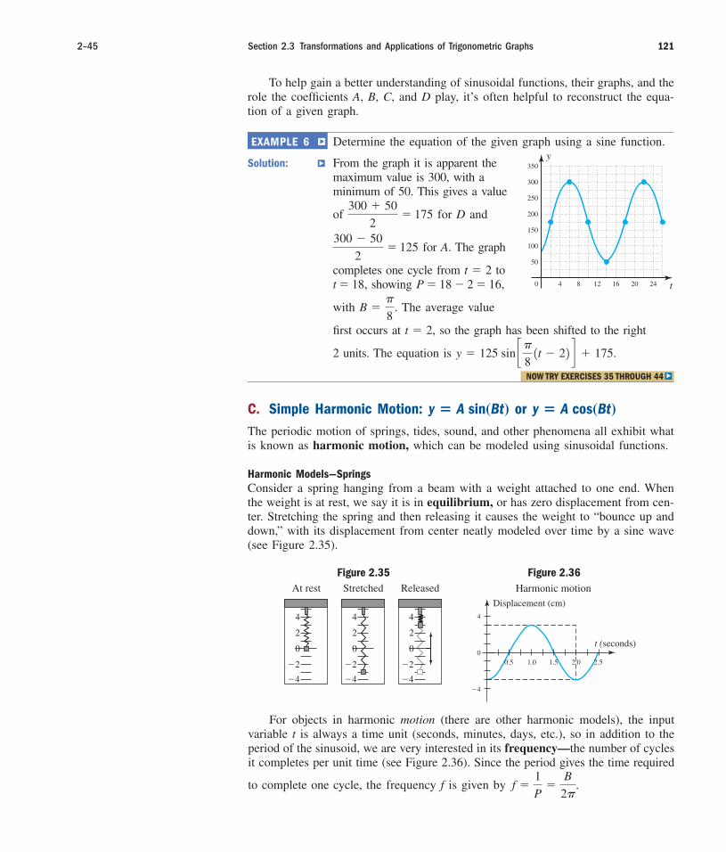
2–45 Section 2.3 Transformations and Applications of Trigonometric Graphs 121
To help gain a better understanding of sinusoidal functions, their graphs, and therole the coefficients A, B, C, and D play, it’s often helpful to reconstruct the equa-tion of a given graph.
▼EXAMPLE 6 Determine the equation of the given graph using a sine function.
Solution: From the graph it is apparent themaximum value is 300, with aminimum of 50. This gives a value
of for D and
for A. The graph
completes one cycle from toshowing
with The average value
first occurs at so the graph has been shifted to the right
2 units. The equation is y � 125 sin c�8
1t � 22 d � 175.
t � 2,
B ��
8.
P � 18 � 2 � 16,t � 18,t � 2
300 � 50
2� 125
300 � 50
2� 175
24201612840
350
300
250
150
200
100
50
t
y
NOW TRY EXERCISES 35 THROUGH 44 ▼
C. Simple Harmonic Motion: or
The periodic motion of springs, tides, sound, and other phenomena all exhibit whatis known as harmonic motion, which can be modeled using sinusoidal functions.
Harmonic Models—Springs
Consider a spring hanging from a beam with a weight attached to one end. Whenthe weight is at rest, we say it is in equilibrium, or has zero displacement from cen-ter. Stretching the spring and then releasing it causes the weight to “bounce up anddown,” with its displacement from center neatly modeled over time by a sine wave(see Figure 2.35).
y � A cos(Bt)y � A sin(Bt)
0
2
�2
�4
4
At rest
0
2
�2
�4
4
Stretched
0
2
�2
�4
4
Released
0.5 1.0 1.5 2.0 2.5
t (seconds)
Displacement (cm)
Harmonic motion
�4
4
0
Figure 2.35 Figure 2.36
For objects in harmonic motion (there are other harmonic models), the inputvariable t is always a time unit (seconds, minutes, days, etc.), so in addition to theperiod of the sinusoid, we are very interested in its frequency—the number of cyclesit completes per unit time (see Figure 2.36). Since the period gives the time required
to complete one cycle, the frequency f is given by f �1
P�
B
2�.
cob10054_ch02_77-158.qxd 10/12/06 5:04 PM Page 121 CONFIRMING PAGES

▼EXAMPLE 7 For the harmonic motion modeled by the sinusoid in Figure 2.36,(a) find an equation of the form (b) determine thefrequency; and (c) use the equation to find the position of theweight at sec.
Solution: a. By inspection the graph has an amplitude and a period
After substitution into we obtain andthe equation
b. Frequency is the reciprocal of the period so showing
one-half a cycle is completed each second (as the graph indicates).
c. Evaluating the model at gives meaning the weight is 2.43 cm below the equilibrium
point at this time.�2.43,
y � �3 cos 3� 11.82 4 �t � 1.8
f �1
2,
y � �3 cos1�t2. B � �P �2�
B,P � 2.
�A� � 3
t � 1.8
y � A cos1Bt2;
CHAPTER 2 Trigonometric Graphs and Models 2–46122
NOW TRY EXERCISES 47 THROUGH 50 ▼
Harmonic Models—Sound Waves
A second example of harmonic motion is the production of sound. For the pur-poses of this study, we’ll look at musical notes. The vibration of matter producesa pressure wave or sound energy, which in turn vibrates the eardrum. Throughthe intricate structure of the middle ear, this sound energy is converted intomechanical energy and sent to the inner ear where it is converted to nerveimpulses and transmitted to the brain. If the sound wave has a high frequency,the eardrum vibrates with greater frequency, which the brain interprets as a “high-pitched” sound. The intensity of the sound wave can also be transmitted tothe brain via these mechanisms, and if the arriving sound wave has a high ampli-tude, the eardrum vibrates more forcefully and the sound is interpreted as“loud” by the brain. These characteristics are neatly modeled using For the moment we will focus on the frequency, keeping the amplitude constantat
The musical note known as or “the A above middle C” is produced with a fre-quency of 440 vibrations per second, or 440 hertz (Hz) (this is the note most often usedin the tuning of pianos and other musical instruments). For any given note, the same noteone octave higher will have double the frequency, and the same note one octave lower
will have one-half the frequency. In addition, with the value of can
always be expressed as so has the equation (afterrearranging the factors). The same note one octave lower is and has the equa-tion , with one-half the frequency. To draw the representativegraphs, we must scale the t-axis in very small increments (seconds � ) since
for and for Both are graphed in A3.P �1
220� 0.0045A 4,P �
1
440� 0.0023
10�3sin 322012�t2 4y �
A3
y � sin 344012�t2 4A4B � 2�f,
B � 2� a 1
Pbf �
1
P
A4
A � 1.
y � A sin1Bt2.
cob10054_ch02_77-158.qxd 10/12/06 5:04 PM Page 122 CONFIRMING PAGES
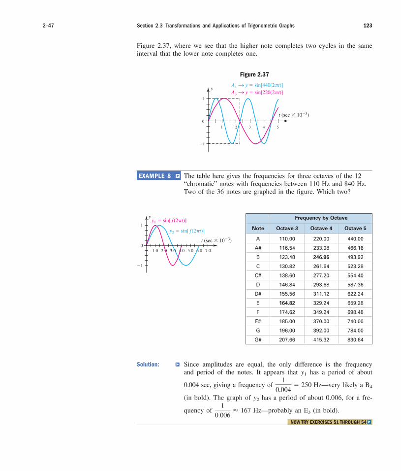
▼EXAMPLE 8 The table here gives the frequencies for three octaves of the 12“chromatic” notes with frequencies between 110 Hz and 840 Hz.Two of the 36 notes are graphed in the figure. Which two?
2–47 Section 2.3 Transformations and Applications of Trigonometric Graphs 123
Figure 2.37
1 2 3 4 5
t (sec � 10�3)
A4 y � sin[440(2�t)]y
�1
1
0
A3 y � sin[220(2�t)]
Frequency by Octave
Note Octave 3 Octave 4 Octave 5
A 110.00 220.00 440.00
A# 116.54 233.08 466.16
B 123.48 246.96 493.92
C 130.82 261.64 523.28
C# 138.60 277.20 554.40
D 146.84 293.68 587.36
D# 155.56 311.12 622.24
E 164.82 329.24 659.28
F 174.62 349.24 698.48
F# 185.00 370.00 740.00
G 196.00 392.00 784.00
G# 207.66 415.32 830.64
5.0 6.0 7.0
t (sec � 10�3)
y1 � sin[ f (2�t)]
y2 � sin[ f (2�t)]
y
�1
1
01.0 2.0 3.0 4.0
Solution: Since amplitudes are equal, the only difference is the frequencyand period of the notes. It appears that has a period of about
0.004 sec, giving a frequency of Hz—very likely a
(in bold). The graph of has a period of about 0.006, for a fre-
quency of Hz—probably an (in bold).E31
0.006� 167
y2
B41
0.004� 250
y1
NOW TRY EXERCISES 51 THROUGH 54 ▼
Figure 2.37, where we see that the higher note completes two cycles in the sameinterval that the lower note completes one.
cob10054_ch02_77-158.qxd 10/12/06 5:04 PM Page 123 CONFIRMING PAGES
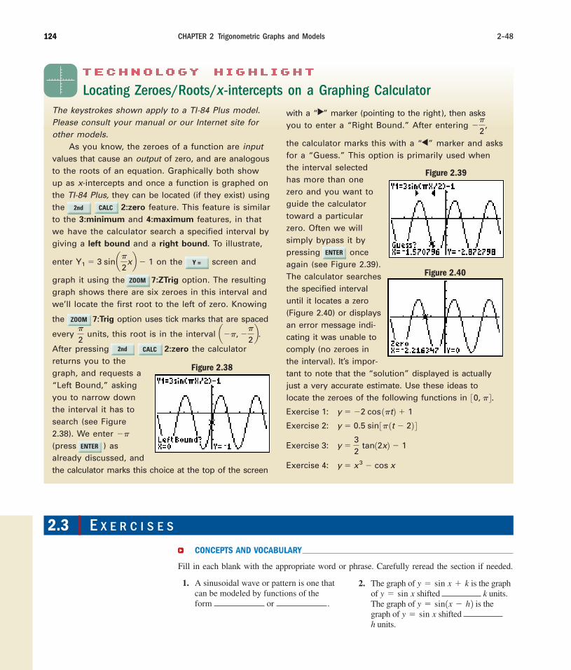
CHAPTER 2 Trigonometric Graphs and Models 2–48124124
TECHNOLOGY H IGHLIGHT
Locating Zeroes/Roots/x-intercepts on a Graphing CalculatorThe keystrokes shown apply to a TI-84 Plus model.
Please consult your manual or our Internet site for
other models.
As you know, the zeroes of a function are input
values that cause an output of zero, and are analogous
to the roots of an equation. Graphically both show
up as x-intercepts and once a function is graphed on
the TI-84 Plus, they can be located (if they exist) using
the 2:zero feature. This feature is similar
to the 3:minimum and 4:maximum features, in that
we have the calculator search a specified interval by
giving a left bound and a right bound. To illustrate,
enter on the screen and
graph it using the 7:ZTrig option. The resulting
graph shows there are six zeroes in this interval and
we’ll locate the first root to the left of zero. Knowing
the 7:Trig option uses tick marks that are spaced
every units, this root is in the interval
After pressing 2:zero the calculator
returns you to the
graph, and requests a
“Left Bound,” asking
you to narrow down
the interval it has to
search (see Figure
2.38). We enter
(press ) as
already discussed, and
the calculator marks this choice at the top of the screen
��
a��, ��
2b.�
2
Y1 � 3 sin a�
2xb � 1
with a “ ” marker (pointing to the right), then asks
you to enter a “Right Bound.” After entering
the calculator marks this with a “ ” marker and asks
for a “Guess.” This option is primarily used when
the interval selected
has more than one
zero and you want to
guide the calculator
toward a particular
zero. Often we will
simply bypass it by
pressing once
again (see Figure 2.39).
The calculator searches
the specified interval
until it locates a zero
(Figure 2.40) or displays
an error message indi-
cating it was unable to
comply (no zeroes in
the interval). It’s impor-
tant to note that the “solution” displayed is actually
just a very accurate estimate. Use these ideas to
locate the zeroes of the following functions in
Exercise 1:
Exercise 2:
Exercise 3:
Exercise 4: y � x 3 � cos x
y �3
2 tan12x2 � 1
y � 0.5 sin 3� 1t � 22 4y � �2 cos 1�t2 � 1
30, � 4 .
▲
��
2,
▲
Figure 2.40
Figure 2.38
Figure 2.39
2nd CALC
Y =
ZOOM
2nd CALC
ENTER
ENTER
CONCEPTS AND VOCABULARY
Fill in each blank with the appropriate word or phrase. Carefully reread the section if needed.
2.3 E X E R C I S E S
1. A sinusoidal wave or pattern is one thatcan be modeled by functions of theform or .
2. The graph of is the graphof shifted k units.The graph of is thegraph of shifted h units.
y � sin xy � sin 1x � h 2y � sin xy � sin x � k
ZOOM
cob10054_ch02_77-158.qxd 10/17/06 4:42 PM Page 124CONFIRMING PAGES

2–49 Exercises 125125
3. To find the primary interval of a sinu-soidal graph, solve the inequality
.
5. Explain/discuss the difference betweenthe standard form of a sinusoidal equa-tion, and the shifted form. How do youobtain one from the other? For whatbenefit?
4. Given the period P, the frequency is, and given the frequency f,
the value of B is .
6. Write out a step-by-step procedure for sketching the graph of
Include
use of the reference rectangle, primary interval, zeroes, max/mins, and so on.Be complete and thorough.
y � 30 sin a�
2 t �
1
2b � 10.
DEVELOPING YOUR SKILLS
Use the graphs given to (a) state the amplitude A and period P of the function; (b) estimatethe value at and (c) estimate the interval in where
7. 8.
Use the graphs given to (a) state the amplitude A and period P of the function; (b) estimatethe value at and (c) estimate the interval in where
9. 10.
Use the information given to write a sinusoidal equation and sketch its graph. Recall
11. Max: 100, min: 20, 12. Max: 95, min: 40,
13. Max: 20, min: 4, 14. Max: 12,000, min: 6500,
Use the information given to write a sinusoidal equation, sketch its graph, and answer thequestion posed.
15. In Geneva, Switzerland, the daily temperature in January ranges from an average high ofto an average low of . (a) Find a sinusoidal equation model for the daily
temperature; (b) sketch the graph; and (c) approximate the time(s) each January day thetemperature reaches the freezing point Assume corresponds to noon.
Source: 2004 Statistical Abstract of the United States, Table 1331.
16. In Nairobi, Kenya, the daily temperature in January ranges from an average high ofto an average low of . (a) Find a sinusoidal equation model for the daily
temperature; (b) sketch the graph; and (c) approximate the time(s) each January daythe temperature reaches a comfortable . Assume corresponds to noon.
Source: 2004 Statistical Abstract of the United States, Table 1331.
17. In Oslo, Norway, the number of hours of daylight reaches a low of 6 hr in January,and a high of nearly 18.8 hr in July. (a) Find a sinusoidal equation model for the
t � 072°F
58°F77°F
t � 0132°F 2.29°F39°F
P � 10P � 360
P � 24P � 30
B �2�
P.
�100
100
21 3 5 74 6 8
f (x)
x
�250
250f (x)
x32
92
154
214
274
94
3 434
f 1x 2 � �100.30, P 4 ,x � 2;
�50
50
30252015105
f (x)
x
�50
50
6 12 18 24 30
f (x)
x
f 1x 2 � 20.30, P 4 ,x � 14;
cob10054_ch02_77-158.qxd 10/17/06 2:06 PM Page 125CONFIRMING PAGES

CHAPTER 2 Trigonometric Graphs and Models 2–50126
number of daylight hours each month; (b) sketch the graph; and (c) approximatethe number of days each year there are more than 15 hr of daylight. Use1 month 30.5 days. Assume corresponds to January 1.
Source: www.visitnorway.com/templates.
18. In Vancouver, British Columbia, the number of hours of daylight reaches a low of8.3 hr in January, and a high of nearly 16.2 hr in July. (a) Find a sinusoidal equa-tion model for the number of daylight hours each month; (b) sketch the graph; and(c) approximate the number of days each year there are more than 15 hr of day-light. Use 1 month 30.5 days. Assume corresponds to January 1.
Source: www.bcpassport.com/vital/temp.
19. Recent studies seem to indicate the population of North American porcupine (Erethizondorsatum) varies sinusoidally with the solar (sunspot) cycle due to its effects onEarth’s ecosystems. Suppose the population of this species in a certain locality is
modeled by the function where P(t) represents the
population of porcupines in year t. Use the model to (a) find the period of the func-tion; (b) graph the function over one period; (c) find the maximum and minimumvalues; and (d) estimate the number of years the population is less than 740 animals.
Source: Ilya Klvana, McGill University (Montreal), Master of Science thesis paper,
November 2002.
20. The population of mosquitoes in a given area is primarily influenced by precipitation,humidity, and temperature. In tropical regions, these tend to fluctuate sinusoidally in thecourse of a year. Using trap counts and statistical projections, fairly accurate estimatesof a mosquito population can be obtained. Suppose the population in a certain region
was modeled by the function where P(t) was the mosquito
population (in thousands) in week t of the year. Use the model to (a) find theperiod of the function; (b) graph the function over one period; (c) find the maxi-mum and minimum population values; and (d) estimate the number of weeks thepopulation is less than 915,000.
21. Use a horizontal translation to shift the graph from Exercise 19 so that the averagepopulation of the North American porcupine begins at Verify results on agraphing calculator, then find a sine function that gives the same graph as theshifted cosine function.
22. Use a horizontal translation to shift the graph from Exercise 20 so that the averagepopulation of mosquitoes begins at t � 0. Verify results on a graphing calculator, thenfind a sine function that gives the same graph as the shifted cosine function.
Identify the amplitude (A), period (P), horizontal shift (HS), vertical shift (VS), and endpointsof the primary interval (PI) for each function given.
23. 24. 25.
26. 27. 28.
29. 30.
31. 32.
33. 34. y � 1450 sin a3�
4 t �
�
8b � 2050y � 2500 sin a�
4 t �
�
12b � 3150
f 1t2 � 90 sin a �
10 t �
�
5b � 120g1t2 � 28 sin a�
6 t �
5�
12b � 92
g1t2 � 40.6 sin c �6
1t � 4 2 d � 13.4f 1t2 � 24.5 sin c �
10 1t � 2.5 2 d � 15.5
y � sin a�
3 t �
5�
12by � sin a�
4 t �
�
6br 1t2 � sin a �
10 t �
2�
5b
h1t2 � sin a�
6 t �
�
3by � 560 sin c �
4 1t � 4 2 dy � 120 sin c �
12 1t � 6 2 d
t � 0.
P1t2 � 50 cos a �
26 tb � 950,
P1t2 � 250 cos a2�
11 tb � 950,
t � 0�
t � 0�
cob10054_ch02_77-158.qxd 10/12/06 5:04 PM Page 126 CONFIRMING PAGES

Find the equation of the graph given. Write answers in the form
35. 36.
37. 38.
39. 40.
Sketch one complete period of each function.
41. 42.
43. 44.
WORKING WITH FORMULAS
45. The relationship between the coefficient B, the frequency f, and the period P
In many applications of trigonometric functions, the equation is written as
where Justify the new equation using and .
In other words, explain how becomes as though you weretrying to help another student with the ideas involved.
46. Number of daylight hours:
The number of daylight hours for a particular day of the year is modeled by the for-mula given, where D(t) is the number of daylight hours on day t of the year and K isa constant related to the total variation of daylight hours, latitude of the location, andother factors. For the city of Reykjavik, Iceland, while for Detroit, Michigan,
How many hours of daylight will each city receive on June 30 (the 182nd dayof the year)?
APPLICATIONS
47. Harmonic motion: A weight on the end of a spring is oscillating in harmonic motion.
The equation model for the oscillations is where d is the distance
(in centimeters) from the equilibrium point in t sec.
a. What is the period of the motion? What is the frequency of the motion?
b. What is the displacement from equilibrium at ? Is the weight moving towardthe equilibrium point or away from equilibrium at this time?
t � 2.5
d 1t2 � 6 sin a�
2 tb,
K � 6.K � 17,
D1t2 �K2
sin c 2�
365 1t � 792 d � 12
A sin 3 12�f 2t 4 ,A sin 1Bt2P �
2�
Bf �
1
PB � 2�f.y � A sin 3 12�f 2t 4 ,
y � A sin 1Bt2
p1t2 � 350 sin a�
6 t �
�
3b � 420h 1t2 � 1500 sin a�
8 t �
�
4b � 7000
g 1t2 � 24.5 sin c �
10 1t � 2.5 2 d � 15.5f 1t2 � 25 sin c �
4 1t � 2 2 d � 55
24 3630181260
6000
5000
4000
3000
2000
1000
x
y
360270180900
12
10
8
6
4
2
x
y
24 30 36181260
120
140
100
80
60
40
20
x
y
100 1257550250
18
20
16
14
12
10
8
x
y
32241680
120
140
100
80
60
40
20
t
y
24181260
600
700
500
400
300
200
100
t
y
y � A sin 1Bt � C 2 � D.
2–51 Exercises 127
cob10054_ch02_77-158.qxd 10/12/06 5:04 PM Page 127 CONFIRMING PAGES

c. What is the displacement from equilibrium at ? Is the weight moving towardthe equilibrium point or away from equilibrium at this time?
d. How far does the weight move between and sec? What is the averagevelocity for this interval? Do you expect a greater or lesser velocity for to
? Explain why.
48. Harmonic motion: The bob on the end of a 24-in. pendulum is oscillating in har-monic motion. The equation model for the oscillations is where d isthe distance (in inches) from the equilibrium point, t sec after being released from oneside.
a. What is the period of the motion? What is the frequency of the motion?
b. What is the displacement from equilibrium at sec? Is the weight movingtoward the equilibrium point or away from equilibrium at this time?
c. What is the displacement from equilibrium at sec? Is the weight movingtoward the equilibrium point or away from equilibrium at this time?
d. How far does the bob move between and sec? What is its averagevelocity for this interval? Do you expect a greater velocity for the interval to ? Explain why.
49. Harmonic motion: A simple pendulum 36 in. in length is oscillating in harmonicmotion. The bob at the end of the pendulum swings through an arc of 30 in. (from thefar left to the far right, or one-half cycle) in about 0.8 sec. What is the equation modelfor this harmonic motion?
50. Harmonic motion: As part of a study of wave motion, the motion of a floater isobserved as a series of uniform ripples of water move beneath it. By careful observa-tion, it is noted that the floater bobs up and down through a distance of 2.5 cm every
sec. What is the equation model for this harmonic motion?
51. Sound waves: Two of the musical notes from the chart on page 123 are graphed inthe figure. Use the graphs given to determine which two.
1
3
t � 0.6t � 0.55
t � 0.35t � 0.25
t � 1.3
t � 0.25
d 1t2 � 20 cos14t2,t � 2
t � 1.75t � 1.5t � 1
t � 3.5
CHAPTER 2 Trigonometric Graphs and Models 2–52128
d d
2 4 6 8 10
t (sec � 10�3)
y1 � sin[ f (2�t)]
y2 � sin[ f (2�t)]y
�1
1
0
0.4 0.8 1.2 1.6 2.0
t (sec � 10�2)
y1 � sin[ f (2�t)]
y2 � sin[ f (2�t)]
y
�1
1
0
52. Sound waves: Two chromatic notes not on the chart from page 123 are graphed in thefigure. Use the graphs and the discussion regarding octaves to determine which two.Note the scale of the t-axis has been changed to hundredths of a second.
cob10054_ch02_77-158.qxd 10/12/06 5:04 PM Page 128 CONFIRMING PAGES

2–53 Exercises 129
Sound waves: Use the chart on page 123 to draw graphs representing each pair of thesenotes. Write the equation for each note in the form and clearly state theperiod of each note.
53. notes and 54. the notes and
Temperature models: Use the information given to determine the amplitude, period, aver-age value (AV), and horizontal shift. Then write the equation and sketch the graph. Assumeeach context is sinusoidal.
55. During a typical January (summer) day in Buenos Aires, Argentina, the daily hightemperature is and the daily low is Assume the low temperature occursaround 6:00 A.M. Assume corresponds to midnight.
56. In Moscow, Russia, a typical January day brings a high temperature of and alow of Assume the high temperature occurs around 4:00 P.M. Assume corresponds to midnight.
Daylight hours model: Solve using a graphing calculator and the formula given inExercise 46.
57. For the city of Caracas, Venezuela, while for Tokyo, Japan,
a. How many hours of daylight will each city receive on January 15th (the 15th day ofthe year)?
b. Graph the equations modeling the hours of daylight on the same screen. Then deter-mine (i) what days of the year these two cities will have the same number of hours ofdaylight, and (ii) the number of days each year that each city receives 11.5 hr or lessof daylight.
58. For the city of Houston, Texas, while for Pocatello, Idaho,
a. How many hours of daylight will each city receive on December 15 (the 349th dayof the year)?
b. Graph the equations modeling the hours of daylight on the same screen. Thendetermine (i) how many days each year Pocatello receives more daylight thanHouston, and (ii) the number of days each year that each city receives 13.5 hr ormore of daylight.
WRITING, RESEARCH, AND DECISION MAKING
59. Some applications of sinusoidal graphs use variable amplitudes and variable fre-quencies, rather than constant values of f and P as illustrated in this section. Theclassic example is AM (amplitude modulated) and FM (frequency modulated) radiowaves. Use the Internet, an encyclopedia, or the resources of a local library toresearch the similarities and differences between AM and FM radio waves, andinclude a sketch of each type of wave. What are the advantages and disadvantagesof each? Prepare a short summary on what you find. For other applications involv-ing variable amplitudes, see the Calculator Exploration and Discovery feature atthe end of this chapter.
60. A laser beam is actually a very narrow beam of light with a constant frequencyand very high intensity (LASER is an acronym for light amplified by stimulatedemission of radiation). Lasers have a large and growing number of practicalapplications, including repair of the eye’s retina, sealing of blood vessels duringsurgery, treatment of skin cancer, drilling small holes, and making precisemeasurements. In the study of various kinds of laser light, sinusoidal equations
K � 6.2.K � 3.8,
K � 4.8.K � 1.3,
t � 011°F.21°F
t � 064°F.84°F
C#3A5G4D3
y � sin 3 f 12�t2 4
cob10054_ch02_77-158.qxd 10/12/06 5:04 PM Page 129 CONFIRMING PAGES

CHAPTER 2 Trigonometric Graphs and Models 2–54130
are used to model certain characteristics of the light emitted. Do some furtherreading and research on lasers, and see if you can locate and discuss some ofthese sinusoidal models.
EXTENDING THE CONCEPT
61. The formulas we use in mathematics can sometimes seem very mysterious. We know they “work,” and we can graph and evaluate them—but where did they come from? Consider the formula for the number of daylight hours from Exercise 46:
a. We know that the addition of 12 represents a vertical shift, but what does a verticalshift of 12 mean in this context?
b. We also know the factor represents a phase shift of 79 to the right. But whatdoes a horizontal (phase) shift of 79 mean in this context?
c. Finally, the coefficient represents a change in amplitude, but what does a change
of amplitude mean in this context? Why is the coefficient bigger for the northernlatitudes?
62. Use a graphing calculator to graph the equation
a. Determine the interval between each peak of the graph. What do you notice?
b. Graph on the same screen and comment on what you observe.
c. What would the graph of look like? What is the
x-intercept?
MAINTAINING YOUR SKILLS
63. (1.1) In what quadrant does the angle terminate? What is the reference arc?
64. (1.3) The planet Venus orbits the Sun in a path that is nearly circular, with a radius of67.2 million miles. Through what angle of its orbit has the planet moved after travel-ing 168 million miles?
65. (1.3) Given with find the value of all six trig functions of
66. (1.4) While waiting for John in the parking lot of the hotel, Rick passes the time byestimating the angle of elevation of the hotel’s exterior elevator. By careful observa-tion, he notes that from an angle of elevation of 20�, it takes the elevator 5 sec untilthe angle grows to 52� and reaches the penthouse floor. If his car is parked 150 ftfrom the hotel, (a) how far does the elevator move during this time? (b) What is theaverage speed (in miles per hour) of the elevator?
67. (1.1) The vertices of a triangle have coordinates (1, 10), and (2, 3). Verifythat a right triangle is formed and find the measures of the two acute angles.
68. (2.1/2.2) Draw a quick sketch of , and for
x � c��
2, 2� d .
y � 2 tan xy � 2 cos xy � 2 sin x,
1�2, 6 2,
�.tan � 6 0,sin � � � 512
t � 3.7
f 1x 2 � �3x
2� 2 sin 12x 2 � 1.5
g1x2 �3x
2� 1.5
f 1x 2 �3x
2� 2 sin 12x 2 � 1.5.
K
2
1t � 79 2
sin c 2�
365 1t � 792 d � 12.D 1t2 �
K
2
cob10054_ch02_77-158.qxd 10/12/06 5:04 PM Page 130 CONFIRMING PAGES
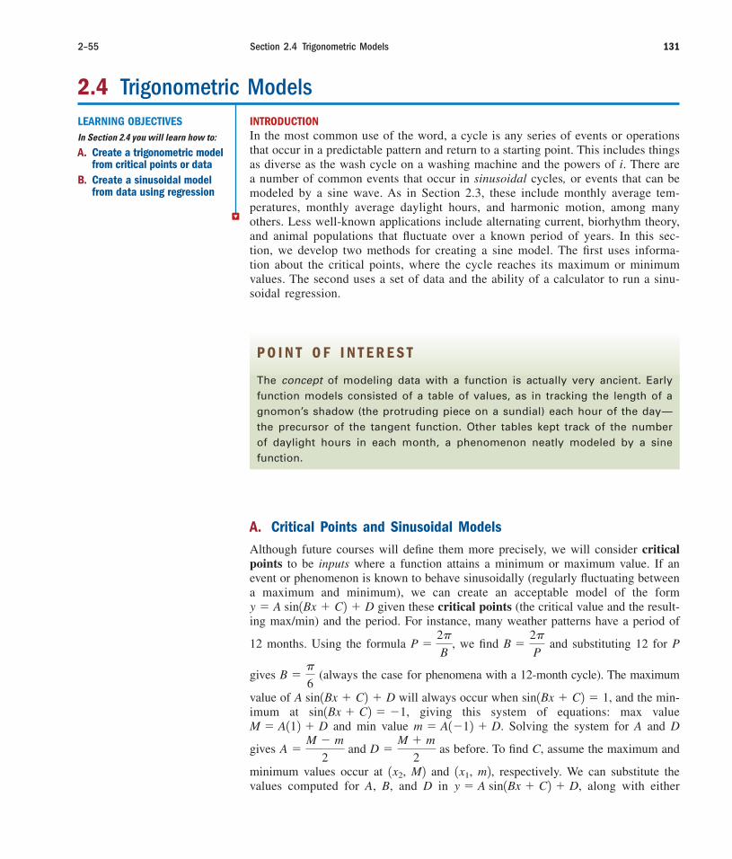
2.4 Trigonometric Models
2–55 Section 2.4 Trigonometric Models 131
INTRODUCTION
In the most common use of the word, a cycle is any series of events or operationsthat occur in a predictable pattern and return to a starting point. This includes thingsas diverse as the wash cycle on a washing machine and the powers of i. There area number of common events that occur in sinusoidal cycles, or events that can bemodeled by a sine wave. As in Section 2.3, these include monthly average tem-peratures, monthly average daylight hours, and harmonic motion, among manyothers. Less well-known applications include alternating current, biorhythm theory,and animal populations that fluctuate over a known period of years. In this sec-tion, we develop two methods for creating a sine model. The first uses informa-tion about the critical points, where the cycle reaches its maximum or minimumvalues. The second uses a set of data and the ability of a calculator to run a sinu-soidal regression.
LEARNING OBJECTIVES
In Section 2.4 you will learn how to:
A. Create a trigonometric modelfrom critical points or data
B. Create a sinusoidal modelfrom data using regression
P O I N T O F I N T E R E S T
The concept of modeling data with a function is actually very ancient. Early
function models consisted of a table of values, as in tracking the length of a
gnomon’s shadow (the protruding piece on a sundial) each hour of the day—
the precursor of the tangent function. Other tables kept track of the number
of daylight hours in each month, a phenomenon neatly modeled by a sine
function.
A. Critical Points and Sinusoidal Models
Although future courses will define them more precisely, we will consider criticalpoints to be inputs where a function attains a minimum or maximum value. If anevent or phenomenon is known to behave sinusoidally (regularly fluctuating betweena maximum and minimum), we can create an acceptable model of the form
given these critical points (the critical value and the result-ing max/min) and the period. For instance, many weather patterns have a period of
12 months. Using the formula we find and substituting 12 for P
gives (always the case for phenomena with a 12-month cycle). The maximum
value of will always occur when and the min-imum at giving this system of equations: max value
and min value Solving the system for A and D
gives and as before. To find C, assume the maximum and
minimum values occur at , M and , m respectively. We can substitute thevalues computed for A, B, and D in along with eithery � A sin1Bx � C2 � D,
2,x112x21D �
M � m
2A �
M � m
2
m � A1�12 � D.M � A112 � Dsin1Bx � C2 � �1,
sin1Bx � C2 � 1,A sin1Bx � C2 � D
B ��
6
B �2�
PP �
2�
B,
y � A sin1Bx � C2 � D
▼
cob10054_ch02_77-158.qxd 12/10/06 16:39 Page 131 CONFIRMING PAGES

▼
, M or , m , and solve for C. Using the minimum value , where and , we have:
sinusoidal equation model
substitute for y and for x
isolate sine function
Fortunately, for sine models constructed from critical points we have
which is always equal to (see Exercise 33). This gives a simple
result for C, since leads to or .
Exercises 7 through 12 offer abundant practice with these ideas. Note how they’re used in the context of an application.
C �3�
2� Bx1
3�
2� Bx1 � C�1 � sin 1Bx1 � C2
�1y � D
A S
m � D
A,
m � D
A� sin1Bx1 � C2
x1m m � A sin1Bx1 � C2 � D y � A sin1Bx � C2 � D
y � mx � x12x1, m12x112x21
CHAPTER 2 Trigonometric Graphs and Models 2–56132
EXAMPLE 1 When the Spirit and Odyssey Rovers landed on Mars (January2004), there was a renewed public interest in studying the planet.Of particular interest were the polar ice caps, which are nowthought to hold frozen water, especially the northern cap. TheMartian ice caps expand and contract with the seasons, just as theydo here on Earth but there are about 687 days in a Martian year,making each Martian “month” just over 57 days long (1 Martianday 1 Earth day). At its smallest size, the northern ice cap coversan area of roughly 0.17 million square miles. At the height of win-ter, the cap covers about 3.7 million square miles (an area aboutthe size of the 50 United States). Suppose these occur at the begin-ning of month 4 x � 4 and month 10 x � 10 respectively.(a) Use this information to create a sinusoidal model of the form
(b) use the model to predict the areaof the ice cap in the eighth Martian month, and (c) use a graphingcalculator to determine the number of months the cap covers lessthan 1 million mi2.
Solution: a. Assuming a “12-month” weather pattern, and
The maximum and minimum points are 10, 3.7 and
Using this information,
and Using gives
The equation model is
where represents
millions of square miles in month x.
f 1x2f 1x2 � 1.765 sin a�
6 x �
5�
6b � 1.935,
C �3�
2�
�
6 142 �
5�
6.
C �3�
2� Bx1,A �
3.7 � 0.17
2� 1.765.
D �3.7 � 0.17
2� 1.93514, 0.172.21
B ��
6.P � 12
f 1x2 � A sin1Bx � C2 � D,
2121
�
W O R T H Y O F N OT E
For a complete review of solvingequations graphically using agraphing calculator, see Appendix II.
cob10054_ch02_77-158.qxd 12/10/06 16:39 Page 132 CONFIRMING PAGES

▼
b. For the size of the cap in month 8 we evaluate the function at
sinusoidal equation model
substitute
evaluate using a calculator
In month 8, the polar ice cap will cover about 2,817,500 mi2.
c. Of the many options available, we opt to solve by locating the
points where and
intersect. After entering the functions on the screen,we set an appropriate window. Here we set and
for a window with a frame around the outputvalues. On the TI-84 Plus, press (CALC)5:intersect to find the intersection points. To four decimalplaces they occur at and The ice capat the northern pole ofMars has an area of less than1 million from early in thesecond month to late in the fifthmonth. The second intersectionis shown in the figure.
mi2
x � 5.9337.x � 2.0663
y � 3�1, 5 4 x � 30, 12 4Y2 � 1Y1 � 1.765 sin a�
6 x �
5�
6b � 1.935
� 2.8175
x � 8 f 182 � 1.765 sin c�6
182 �5�
6d � 1.935
f 1x2 � 1.765 sin a�
6 x �
5�
6b � 1.935
x � 8.
2–57 Section 2.4 Trigonometric Models 133
Y =
2nd TRACE
NOW TRY EXERCISES 15 AND 16 ▼
EXAMPLE 2 Naturalists have found that many animal populations, such as thearctic lynx, some species of fox, and certain rabbit breeds, tendto fluctuate sinusoidally over 10-year periods. Suppose that anextended study of a lynx population began in 1990, and in thethird year of the study, the population had fallen to a minimum of2500. In the eighth year the population hit a maximum of 9500.(a) Use this information to create a sinusoidal model of the form
(b) use the model to predict the lynxpopulation in the year 1996, and (c) use a graphing calculator todetermine the number of years the lynx population is above8000 in a 10-year period.
P 1x2 � A sin1Bx � C2 � D,
While this form of “equation building” can’t match the accuracy of a regressionmodel (computed from a larger set of data), it does lend insight as to how sinusoidalfunctions work. The equation will always contain the maximum and minimum val-ues, and using the period of the phenomena, we can create a smooth sine wave that“fills in the blanks” between these critical points.
cob10054_ch02_77-158.qxd 12/10/06 16:39 Page 133 CONFIRMING PAGES

Solution: a. Since we have Using 1990 as year zero,
the minimum and maximum populations occur at ( ) and
(8, 9500). From the information given,
and Using the minimum value we
have giving an equation model of
where P(x) represents the
lynx population in year x.
b. For the population in 1996 we evaluate the function at
sinusoidal function model
substitute
evaluate using a calculator
In 1996, the lynx population was about 7082.
c. Using a graphing calculator and the functions
and we attempt to
find points of intersection. Enter the functions (press ) andset the viewing window (we used and
). On the TI-84 Plus, press (CALC) 5:intersect to find where and intersect.To four decimal places this occurs at and
The lynx population exceeded 8000 for roughly3 yr. The first intersection is shown.x � 9.5319.
x � 6.4681Y2Y1
y � 30, 10,000 4 x � 30, 12 4
Y2 � 8000,3500 sin a�
5 x �
9�
10b � 6000
Y1 �
� 7082
x � 6 P 162 � 3500 sin c�5
162 �9�
10d � 6000
P 1x2 � 3500 sin a�
5 x �
9�
10b � 6000
x � 6.
P 1x2 � 3500 sin a�
5 x �
9�
10b� 6000,
C �3�
2�
�
5 132 �
9�
10,
A �9500 � 2500
2� 3500.
D �9500 � 2500
2� 6000,
3, 2500
B �2�
10�
�
5.P � 10,
CHAPTER 2 Trigonometric Graphs and Models 2–58134
Y =
2nd TRACE
NOW TRY EXERCISES 17 AND 18 ▼
This type of equation building isn’t limited to the sine function, in fact there aremany situations where a sine model cannot be applied. Consider the length of theshadows cast by a flagpole or radio tower as the Sun makes its way across the sky.The shadow’s length follows a regular pattern (shortening then lengthening) and“always returns to a starting point,” yet when the Sun is low in the sky the shadowbecomes (theoretically) infinitely long, unlike the output values from a sine function.In this case, an equation involving might provide a good model, although thedata will vary greatly depending on latitude. We’ll attempt to model the data using
with the D-term absent since a vertical shift in this context has
no meaning. Recall that the period of the tangent function is and that
gives the magnitude and direction of the horizontal shift, in a direction opposite thesign.
�C
BP �
�
�B�
y � A tan1Bx � C2,tan x
cob10054_ch02_77-158.qxd 12/10/06 16:39 Page 134 CONFIRMING PAGES
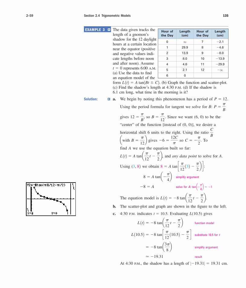
▼
2–59 Section 2.4 Trigonometric Models 135
EXAMPLE 3 The data given tracks the length of a gnomon’sshadow for the 12 daylighthours at a certain locationnear the equator (positiveand negative values indi-cate lengths before noonand after noon). Assume
represents 6:00 A.M.(a) Use the data to findan equation model of theform (b) Graph the function and scatter-plot.(c) Find the shadow’s length at 4:30 P.M. (d) If the shadow is6.1 cm long, what time in the morning is it?
Solution: a. We begin by noting this phenomenon has a period of
Using the period formula for tangent we solve for B:
gives so Since we want (6, 0) to be the
“center” of the function [instead of (0, 0)], we desire a
horizontal shift 6 units to the right. Using the ratio
with gives so To
find A we use the equation built so far:
and any data point to solve for A.
Using ( we obtain
simplify argument
solve for A:
The equation model is
b. The scatter-plot and graph are shown in the figure to the left.
c. 4:30 P.M. indicates Evaluating L(10.5) gives
function model
substitute 10.5 for t
simplify argument
result
At 4:30 P.M., the shadow has a length of cm.��19.31� � 19.31
� �19.31
� �8 tan a3�
8b
L 110.52 � �8 tan c �
12 110.52 �
�
2d
L 1t2 � �8 tan a �
12 t �
�
2b
t � 10.5.
L 1t2 � �8 tan a �
12 t �
�
2b.
tan a��
4b � �1 �8 � A
8 � A tan a��
4b
8 � A tan c �
12 132 �
�
2b d :3, 82
L 1t2 � A tan a �
12 t �
�
2b,
C � ��
2.�6 �
12C�
B ��
12ba
C
B
B ��
12.12 �
�
B,
P ��
B
P � 12.
L 1t2 � A tan1Bt � C2.
t � 0
Hour of Length Hour of Lengththe Day (cm) the Day (cm)
0 7
1 29.9 8
2 13.9 9
3 8.0 10
4 4.6 11
5 2.1 12
6 0
�q
�29.9
�13.9
�8.0
�4.6
�2.1q
cob10054_ch02_77-158.qxd 12/10/06 16:40 Page 135 CONFIRMING PAGES

▼
d. Substituting 6.1 for andsolving for t graphically givesthe graph shown, where we notethe day is about 3.5 hr old—it isabout 9:30 A.M.
L 1t2
CHAPTER 2 Trigonometric Graphs and Models 2–60136
EXAMPLE 4 The data shown givethe record high tem-perature for selectedmonths for Bismarck,North Dakota. (a) Usethe data to draw ascatter-plot, then finda sinusoidal regressionmodel and graph both on the same screen. (b) Use the equationmodel to estimate the record high temperatures for months 2, 6,and 8. (c) Determine what month gives the largest differencebetween the actual data and the computed results. Source: NOAA Comparative Climate Data 2004.
Solution: a. Entering the data and running the regression results in thecoefficients shown in Figure 2.41. After entering the equationin and pressing 9:Zoom Stat we obtain the graphshown in Figure 2.42.
Y1
Figure 2.41 Figure 2.42
NOW TRY EXERCISES 19 THROUGH 22 ▼
B. Data and Sinusoidal Regression
Most graphing calculators are programmed to handle numerous forms of polynomialand nonpolynomial regression, including sinusoidal regression. The sequence ofsteps used is the same regardless of the form chosen, and the fundamentals arereviewed in Appendix III. Exercises 23 through 26 offer further practice with regres-sion fundamentals. Example 4 illustrates their use in context.
Month Temp. Month Temp.(Jan 1) ( F) (Jan 1) ( F)
1 63 9 105
3 81 11 79
5 98 12 65
7 109
�S�S
ZOOM
cob10054_ch02_77-158.qxd 12/10/06 16:40 Page 136 CONFIRMING PAGES
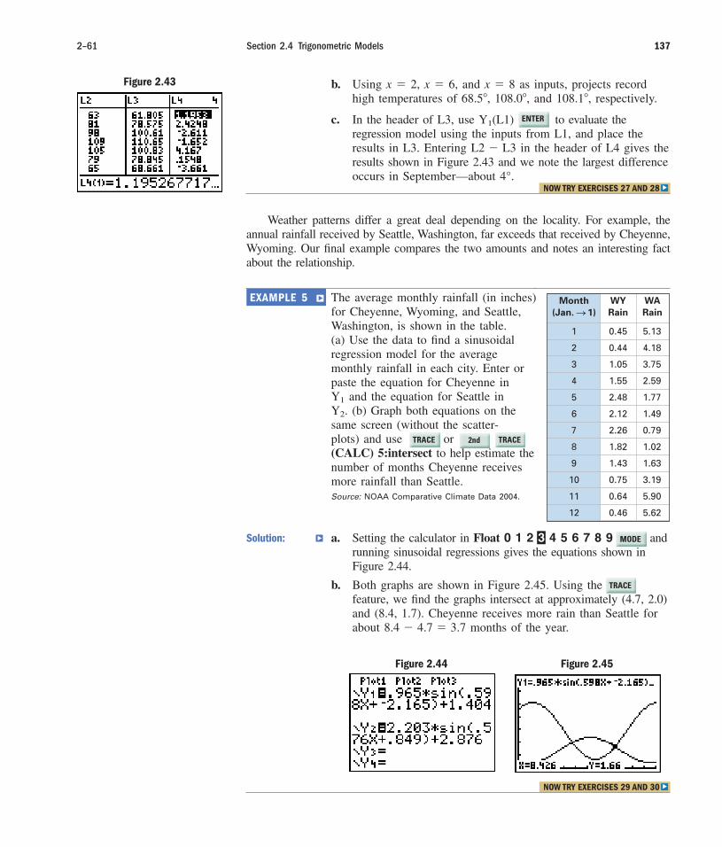
▼
b. Using x � 2, x � 6, and x � 8 as inputs, projects recordhigh temperatures of 68.5�, 108.0�, and 108.1�, respectively.
c. In the header of L3, use (L1) to evaluate theregression model using the inputs from L1, and place theresults in L3. Entering in the header of L4 gives theresults shown in Figure 2.43 and we note the largest differenceoccurs in September—about .4°
L2 � L3
Y1
2–61 Section 2.4 Trigonometric Models 137
Figure 2.43
Weather patterns differ a great deal depending on the locality. For example, theannual rainfall received by Seattle, Washington, far exceeds that received by Cheyenne,Wyoming. Our final example compares the two amounts and notes an interesting factabout the relationship.
EXAMPLE 5 The average monthly rainfall (in inches)for Cheyenne, Wyoming, and Seattle,Washington, is shown in the table.(a) Use the data to find a sinusoidalregression model for the averagemonthly rainfall in each city. Enter orpaste the equation for Cheyenne in
and the equation for Seattle in(b) Graph both equations on the
same screen (without the scatter-plots) and use or(CALC) 5:intersect to help estimate thenumber of months Cheyenne receivesmore rainfall than Seattle.Source: NOAA Comparative Climate Data 2004.
Solution: a. Setting the calculator in Float 0 1 2 3 4 5 6 7 8 9 andrunning sinusoidal regressions gives the equations shown inFigure 2.44.
b. Both graphs are shown in Figure 2.45. Using thefeature, we find the graphs intersect at approximately (4.7, 2.0)and (8.4, 1.7). Cheyenne receives more rain than Seattle forabout months of the year.8.4 � 4.7 � 3.7
Y2.Y1
Month WY WA (Jan. 1) Rain Rain
1 0.45 5.13
2 0.44 4.18
3 1.05 3.75
4 1.55 2.59
5 2.48 1.77
6 2.12 1.49
7 2.26 0.79
8 1.82 1.02
9 1.43 1.63
10 0.75 3.19
11 0.64 5.90
12 0.46 5.62
S
Figure 2.44 Figure 2.45
NOW TRY EXERCISES 29 AND 30 ▼
TRACE
TRACE
MODE
2nd TRACE
ENTER
NOW TRY EXERCISES 27 AND 28 ▼
cob10054_ch02_77-158.qxd 12/10/06 16:40 Page 137 CONFIRMING PAGES

The exercise set offers additional significant and interesting applications, andmany more can be found by searching the Internet for data generated by sinu-soidal phenomena.
CHAPTER 2 Trigonometric Graphs and Models 2–62138
TECHNOLOGY H IGHLIGHT
Working with Data—Common “Breaks and Fixes”The keystrokes illustrated refer to a Plus model.
For other models please consult your manual or visit
our Internet site.
In the process of using a calculator to explore
data sets, extensive work is done with lists, regres-
sions, equations, tables, and graphs, with these and
other features combined. With so many ideas working
together, it helps to be aware of the most common
mistakes and how to correct them. The following list
is not exhaustive, but could prove helpful when using
graphing and calculating technology in support of
your studies.
1. Break: You accidently skip a data entry;
Fix: (INS).
The calculator will insert a new position between
the cursor location and the previous datum.
2. Break: You enter data in the wrong list, say L2
instead of L1; Fix: Use
Place the cursor in the heading of List1 and
press (L2) . The calculator
will automatically copy the contents of L2 into
L1. You can then overwrite or the entries
in L2.
3. Break: You accidently delete a List name;
Fix: Reset List names using 5:SetUpEditor.Using 5:SetUpEditor will reset list names
to the default L1 through L6, without affecting
the data in any list. Use with caution in case you
have Lists stored under custom names.
4. Break: You get the message ERR:DIM MISMATCH;
Fix: several.
This usually occurs when the lists used to run
a regression have an unequal number of
entries (one was overlooked or accidently
L1 � L2.
TI-84 deleted). The primary fix is to double-check the
Lists and find the missing entry. If you are
investigating the regression equation and no
longer need a scatter-plot, try turning the plots
off ( (STATPLOT)) so the calculator
won’t recognize the lists.
5. Break: The axes do not show up on the
screen; Fix: AXESON.
Some programs run on the TI will “turn-off” the
axes so they don’t interfere with how the program
is displayed. Just turn them back on.
6. Break: You get the message ERR:WINDOWRANGE; Fix: reset window size.
This occurs if you accidently enter
(other situations as well).
Simply double-check and correct the entries for
window size.
7. Break: You get the message ERR:domain;
Fix: check context/adjust data.
Most of the time this happens when the form of
regression you’ve chosen can’t use zero entries.
Rethink the context of the data and try another
form of regression, or replace the zero with 0.001.
(Use with caution! and sometimes
results can be significantly affected.)
Exercise 1: In Example 4, suppose the entry was
accidently skipped when inputting the data.
Do you place the cursor on the 81 or the
109 before pressing (INS)?
Exercise 2: While working through Example 5,
the temperatures for Seattle were
accidently listed in L1 instead of L3
where you wanted them. How do you
move the entries to L3?
98°
0 � 0.001
Ymin or Xmax 6 Xmin
Ymax 6DEL2nd
2nd
2nd
2nd DEL
Y=
GRAPH
zoom
2nd ENTER
DEL
STAT
2
cob10054_ch02_77-158.qxd 12/10/06 16:40 Page 138 CONFIRMING PAGES

2–63 Exercises 139
2.4 E X E R C I S E S
CONCEPTS AND VOCABULARY
Fill in each blank with the appropriate word or phrase. Carefully reread the section if needed.
1. For themaximum value occurs when
� 1, leaving y � .
3. For the value
of C is found using
where x is a point.
C �3�
2� Bx,
y � A sin 1Bx � C2 � D,
y � A sin 1Bx � C2 � D, 2. For the mini-mum value occurs when �
leaving y � .
4. Any phenomenon with sinusoidal behavior regularly fluctuates between a
and value.
�1,
y � A sin 1Bx � C2 � D,
5. Rework Example 1, but this time use the maximum value in the calculation for C. Dothe equations differ? Discuss/explain why either critical point can be used to build theequation model.
6. Discuss/explain: (a) How is data concerning average rainfall related to the averagedischarge rate of rivers? (b) How is data concerning average daily temperature relatedto water demand? Are both sinusoidal with the same period? Are there other associa-tions you can think of?
DEVELOPING YOUR SKILLS
Find the sinusoidal equation for the information as given.
7. minimum value at (9, 25); maximumvalue at (3, 75); period: 12 min
9. minimum value at (15, 3); maximumvalue at (3, 7.5); period: 24 hr
11. minimum value at (5, 279); maximumvalue at (11, 1285); period: 12 yr
8. minimum value at (4.5, 35); maximumvalue at (1.5, 121); period: 6 yr
10. minimum value at (3, 3.6); maximumvalue at (7, 12); period: 8 hr
12. minimum value at (6, 8280); maximumvalue at (22, 23,126); period: 32 yr
WORKING WITH FORMULAS
13. Orbiting distance north or south ofthe equator: Unless a satellite is placed in a strictequatorial orbit, its distance north orsouth of the equator will vary accordingto the sinusoidal model shown, whereD(t) is the distance t min after enteringorbit. Negative values indicate it issouth of the equator, and the distance Dis actually a two-dimensional distance,as seen from a vantage point in outer space. The value of B depends on the speed ofthe satellite and the time it takes to complete one orbit, while represents the maxi-mum distance from the equator. (a) Find the equation model for a satellite whose maxi-mum distance north of the equator is 2000 miles and that completes one orbit every2 hr ( ). (b) How many minutes after entering orbit is the satellite directlyabove the equator ? (c) Is the satellite north or south of the equator 257 minafter entering orbit? How far north or south?
14. Biorhythm theory: Advocates of biorhythm theory believe that human beings are influenced by certainbiological cycles that begin at birth, have different periods, and continue throughout
P (d ) � 50 sin(Bd ) � 50
3D1t2 � 0 4P � 120
�A�
D (t) � A cos(Bt)
cob10054_ch02_77-158.qxd 12/10/06 16:40 Page 139 CONFIRMING PAGES

life. The classical cycles and their periods are physical potential (23 days), emotionalpotential (28 days), and intellectual potential (33 days). On any given day of life, thepercent of potential in these three areas is purported to be modeled by the functionshown, where P(d) is the percent of available potential on day d of life. Find the valueof B for each of the physical, emotional, and intellectual potentials and use it to seewhat the theory has to say about your potential today. Use day since last birthday.
APPLICATIONS
15. The U.S. National Oceanic and Atmospheric Administration (USNOAA) keeps temper-ature records for most major U.S. cities. For Phoenix, Arizona, they list an averagehigh temperature of F for the month of January (month 1) and an average hightemperature of F for July (month 7). Assuming January and July are the coolestand warmest months of the year, (a) build a sinusoidal function model for tempera-tures in Phoenix, and (b) use the model to find the average high temperature in Sep-tember. (c) If a person has a tremendous aversion to temperatures over duringwhat months should they plan to vacation elsewhere?
16. Much like the polar ice cap on Mars, thesea ice that surrounds the continent ofAntarctica (the Earth’s southern polar cap)varies seasonally, from about 8 million mi2 inSeptember to about 1 million mi2 in March.Use this information to (a) build a sinusoidalequation that models the advance and retreat ofthe sea ice, and (b) determine the size of theice sheet in May. (c) Find the months ofthe year that the sea ice covers more than6.75 million mi2.
17. A phenomenon is said to be circadian if itoccurs in 24-hr cycles. A person’s body tem-perature is circadian, since there are normallysmall, sinusoidal variations in body tempera-ture from a low of to a high of throughout a 24-hr day. Use this informationto (a) build the circadian equation for a per-son’s body temperature, given corre-sponds to midnight and that a person usuallyreaches their minimum temperature at 5 A.M.;(b) find the time(s) during a day when a person reaches “normal” body temperature
and (c) find the number of hours each day that body temperature is or less.
18. For an internal combustion engine, the position of a piston in the cylinder can be mod-eled by a sinusoidal function. For a particular engine size and idle speed, the pistonhead is 0 in. from the top of the cylinder (the minimum value) when at thebeginning of the intake stroke, and reaches a maximum distance of 4 in. from the topof the cylinder (the maximum value) when sec at the beginning of the compres-sion stroke. Following the compression stroke is the power stroke the exhauststroke and the intake stroke after which it all begins again. Giventhe period of a four-stroke engine under these conditions is second, (a) find thesinusoidal equation modeling the position of the piston, and (b) find the distance ofthe piston from the top of the cylinder at sec. Which stroke is the engine in atthis moment?
t � 19
P � 124
1t � 448 2,1t � 3
48 2,1t � 2
48 2,t � 1
48
t � 0
98.4°F198.6°2;
t � 0
99°F98.2°F
95°,
104.2°65.0°
d � 365.25 1age 2 � days
CHAPTER 2 Trigonometric Graphs and Models 2–64140
Ice caps
mininum
maximum
Exercise 16
cob10054_ch02_77-158.qxd 12/10/06 16:40 Page 140 CONFIRMING PAGES

x y x y
1 2.1
2 6.8
3 15.3
4 25.4
4.5 59
0 0
�1.9�1
�7.2�2
�14.8�3
�26�4
�61�4.5
Exercise 21
2–65 Exercises 141
x y x y
0 7
1 20 8
2 9.7 9
3 5.2 10
4 3 11
5 1.4 12
6 0
�q
�20
�9.7
�5.2
�3
�1.4q
x y x y
0 7 6.4
1 8 13.7
2 9 23.7
3 10 44.3
4 11 91.3
5 12
6 0
q�6.4
�13.7
�23.7
�44.3
�91.3
q
21. While driving toward a Midwestern town on a long, flat stretch of highway, Idecide to pass the time by measuring the apparent height of the tallest building inthe downtown area as I approach. At the time the idea occurred to me, the build-ings were barely visible. Three miles later I hold a 30 cm ruler up to my eyes atarm’s length, and the apparent height of the tallest building is 1 cm. After threemore miles the apparent height is 1.8 cm. Measurements are taken every 3 miuntil I reach town and are shown in the table (assume I was 24 mi from the park-ing garage when I began this activity). (a) Use the data to come up with a tangentfunction model of the building’s apparent height after traveling a distance of x micloser. (b) What was the apparent height of the building at after I had driven19 mi? (c) How many miles had I driven when the apparent height of the buildingtook up all 30 cm of my ruler?
22. The theory of elastic rebound has been used by seismologists to study the cause ofearthquakes. As seen in the figure, the Earth’s crust is stretched to a breaking point bythe slow movement of one tectonic plate in a direction opposite the other along a faultline, and when the rock snaps—each half violently rebounds to its original alignmentcausing the Earth to quake.
Distance HeightTraveled (mi) (cm)
0 0
3 1
6 1.8
9 2.8
12 4.2
15 6.3
18 10
21 21
24 q
Use the data given to find an equation model of the form Then graph thefunction and scatter plot to help find (a) the output for and (b) the value of x where
19. 20.
f 1x2 � 16.x � 2.5
f 1x2� A tan 1Bx � C2.
After yearsof movement
Elasticrebound
POP!
Fault line
Stress line
Start
(0, 0)
0Intake
1234
01234
01234
Compression01234
cob10054_ch02_77-158.qxd 12/10/06 16:40 Page 141 CONFIRMING PAGES
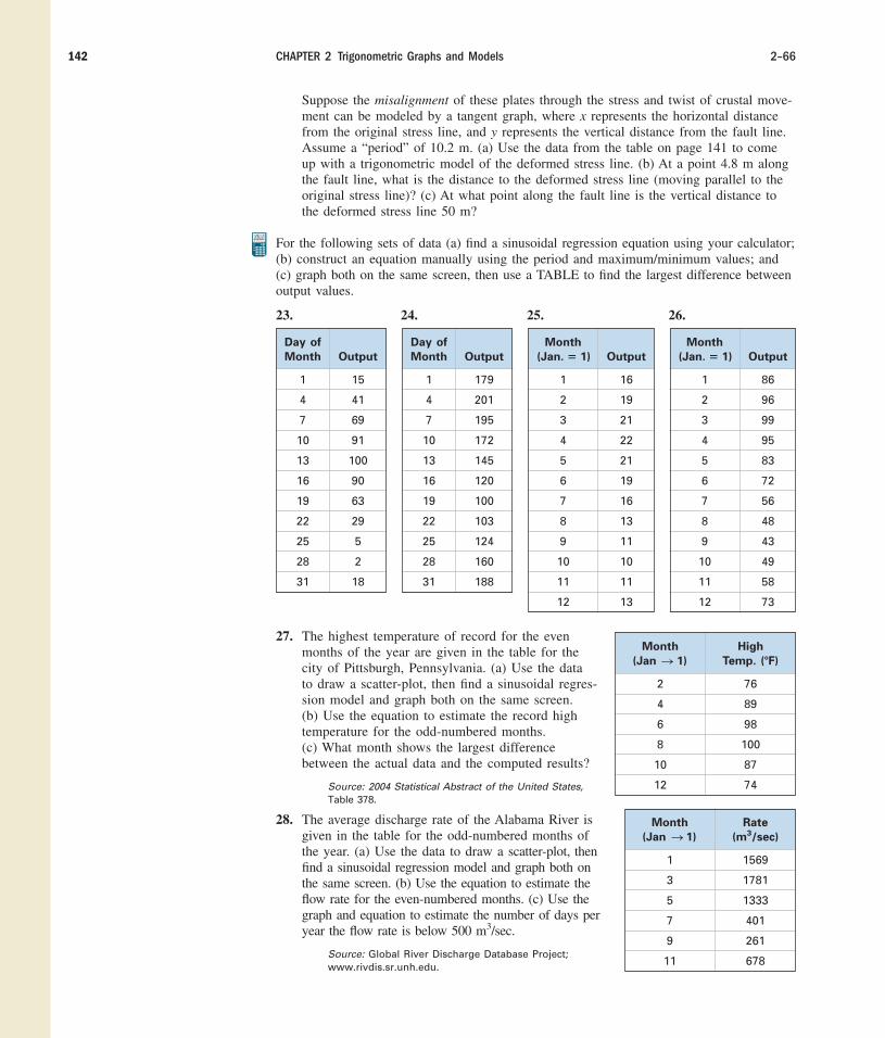
CHAPTER 2 Trigonometric Graphs and Models 2–66142
Suppose the misalignment of these plates through the stress and twist of crustal move-ment can be modeled by a tangent graph, where x represents the horizontal distancefrom the original stress line, and y represents the vertical distance from the fault line.Assume a “period” of 10.2 m. (a) Use the data from the table on page 141 to comeup with a trigonometric model of the deformed stress line. (b) At a point 4.8 m alongthe fault line, what is the distance to the deformed stress line (moving parallel to theoriginal stress line)? (c) At what point along the fault line is the vertical distance tothe deformed stress line 50 m?
For the following sets of data (a) find a sinusoidal regression equation using your calculator;(b) construct an equation manually using the period and maximum/minimum values; and(c) graph both on the same screen, then use a TABLE to find the largest difference betweenoutput values.
23. 24. 25. 26.
Day ofMonth Output
1 15
4 41
7 69
10 91
13 100
16 90
19 63
22 29
25 5
28 2
31 18
Day ofMonth Output
1 179
4 201
7 195
10 172
13 145
16 120
19 100
22 103
25 124
28 160
31 188
Month(Jan. � 1) Output
1 16
2 19
3 21
4 22
5 21
6 19
7 16
8 13
9 11
10 10
11 11
12 13
Month(Jan. � 1) Output
1 86
2 96
3 99
4 95
5 83
6 72
7 56
8 48
9 43
10 49
11 58
12 73
27. The highest temperature of record for the evenmonths of the year are given in the table for thecity of Pittsburgh, Pennsylvania. (a) Use the datato draw a scatter-plot, then find a sinusoidal regres-sion model and graph both on the same screen.(b) Use the equation to estimate the record hightemperature for the odd-numbered months.(c) What month shows the largest differencebetween the actual data and the computed results?
Source: 2004 Statistical Abstract of the United States,
Table 378.
28. The average discharge rate of the Alabama River isgiven in the table for the odd-numbered months ofthe year. (a) Use the data to draw a scatter-plot, thenfind a sinusoidal regression model and graph both onthe same screen. (b) Use the equation to estimate theflow rate for the even-numbered months. (c) Use thegraph and equation to estimate the number of days peryear the flow rate is below 500 m3/sec.
Source: Global River Discharge Database Project;
www.rivdis.sr.unh.edu.
Month High (Jan ) Temp. ( F)
2 76
4 89
6 98
8 100
10 87
12 74
�S 1
Month Rate(Jan ) (m3/sec)
1 1569
3 1781
5 1333
7 401
9 261
11 678
S 1
cob10054_ch02_77-158.qxd 12/10/06 16:40 Page 142 CONFIRMING PAGES

Exercise 30
2–67 Exercises 143
29. The average monthly rainfall (in inches)for Reno, Nevada, is shown in the table.(a) Use the data to find a sinusoidalregression model for the monthly rain-fall. (b) Graph this equation modeland the rainfall equation model forCheyenne, Wyoming (from Example 5),on the same screen, and estimate thenumber of months that Reno gets morerainfall than Cheyenne.
Source: NOAA Comparative Climate Data 2004.
30. The number of daylight hours per month (asmeasured on the 15th of each month) is shown inthe table for the cities of Beaumont, Texas, andMinneapolis, Minnesota. (a) Use the data to find asinusoidal regression model of the daylight hoursfor each city. (b) Graph both equations on thesame screen and use the graphs to estimate thenumber of days each year that Beaumont receivesmore daylight than Minneapolis (use 1 month �30.5 days).
Source: www.encarta.msn.com/media_701500905/
Hours_of_Daylight_by_Latitude.html.
31. The table given indicates the percent of the Moonthat is illuminated for the days of a particularmonth, at a given latitude. (a) Use a graphingcalculator to find a sinusoidal regression model.(b) Use the model to determine what percent ofthe Moon is illuminated on day 20. (c) Use themaximum and minimum values with the periodand an appropriate horizontal shift to create your own model of the data. How do thevalues for A, B, C, and D compare?
32. The mood of persons with SAD syndrome (seasonal affective disorder) often dependson the weather. Victims of SAD are typically more despondent in rainy weather thanwhen the Sun is out, and more comfortable in the daylight hours than at night. Thetable shows the average number of daylight hours for Vancouver, British Columbia,for 12 months of a year. (a) Use a calculator to find a sinusoidal regression model.(b) Use the model to estimate the number of days per year (use 1 month 30.5 days)with more than 14 hr of daylight. (c) Use the maximum and minimum values with theperiod and an appropriate horizontal shift to create a model of the data. How do thevalues for A, B, C, and D compare?
Source: Vancouver Climate at www.bcpassport.com/vital.
�
Month TX MN(Jan 1) Sunlight Sunlight
1 10.4 9.1
2 11.2 10.4
3 12.0 11.8
4 12.9 13.5
5 14.4 16.2
6 14.1 15.7
7 13.9 15.2
8 13.3 14.2
9 12.4 12.6
10 11.5 11.0
11 10.7 9.6
12 10.2 8.7
S
Month Reno Month Reno(Jan 1) Rainfall (Jan 1) Rainfall
1 1.06 7 0.24
2 1.06 8 0.27
3 0.86 9 0.45
4 0.35 10 0.42
5 0.62 11 0.80
6 0.47 12 0.88
SS
Exercise 31
Day % Illum. Day % Illum.
1 28 19 34
4 55 22 9
7 82 25 0
10 99 28 9
13 94 31 30
16 68
Exercise 32
Month Hours Month Hours
1 8.3 7 16.2
2 9.4 8 15.1
3 11.0 9 13.5
4 12.9 10 11.7
5 14.6 11 9.9
6 15.9 12 8.5
cob10054_ch02_77-158.qxd 10/17/06 4:05 PM Page 143CONFIRMING PAGES

CHAPTER 2 Trigonometric Graphs and Models 2–68144
x y x y
4.64 1.33
3.14 1.02
2.04 1.0913�
4
�
4
9�
4�
3�
4
5�
4�
7�
4
MAINTAINING YOUR SKILLS
36. (2.2) Draw a quick sketch of for .
37. (1.3) What four values of t satisfy the equation ?
38. (2.3) Determine the equation of the graph shown, given it’s ofthe form
39. (2.2) The graph of is shifted to the right units. What is the equation of the
shifted graph?
40. (1.2) Clarke is standing between two tall buildings. The angle of elevation to the topof the building to her north is while the angle of elevation to the top of the build-ing to her south is . If she is 400 m from the northern building and 200 m fromthe southern building, which one is taller?
41. (1.1) Lying on his back in three inches of newly fallen snow, Mitchell stretches outhis arms and moves them back and forth (like a car’s wiper blades) to form a snowangel. If his arms are 24 in. long and move through an angle of at the shoulders,what is the area of the angel’s wings that are formed?
35°
70°60°,
�
3y � sec x
y � A cos1Bt ; C2 � D.
| cos t | �1
2
x � c�3�
2, 2� dy � �tan x
�6
0
6
4 8 12 16
y
t
WRITING, RESEARCH, AND DECISION MAKING
33. For the equations from Examples 1 and 2, use the minimum value (x, m) to show that
is equal to Then verify this relationship in general by substituting
for A, for D.
34. Unlike the rainfall data from Example 5, precipitation models are often valid for onlypart of the year, usually during an annual rainy season. Using the Internet or theresources of a local library, do some research on rainfall patterns and construct a sinu-soidal exercise of your own.
EXTENDING THE CONCEPT
35. A dampening factor is any function whose product with a sinusoidal function causes asystematic change in amplitude. In the graph shown, is dampened by the
function Notice the peaks and valleys of the sine graph are points on
the graph of this line. The table given shows points of intersection for andanother dampening factor. Use the regression capabilities of a graphing calculator tofind its equation and graph both functions on the same screen.
y � sin13x2y � �
1
4 x � 2.
y � sin13x2
M � m
2
M � m
2
�1.y � D
AS m � D
A
Exercise 38
cob10054_ch02_77-158.qxd 12/10/06 16:40 Page 144 CONFIRMING PAGES

145
KEY CONCEPTS
• On a unit circle, and Graphing these functions using the x- andy-coordinates of points on the unit circle, results in a periodic, wavelike graph withdomain 1�q, q 2.
sin t � y.cos t � x
SECTION 2.1 Graphs of the Sine and Cosine Functions
▼
S U M M A R Y A N D C O N C E P T R E V I E W ▼
cos t
�2
�
�6
�0.5
�1
1
0.5
� , 0.87� �4� , 0.71�
�3� , 0.5�
�2� , 0�
2� t
Decreasing
3�2
(0, 0)
(0, 0) 3�2
�2
�
�6
�0.5
�1
1
0.5
� , 0.5� �4� , 0.71�
�3� , 0.87�
�2� , 1�
2�
Increasing
t
sin t
• The characteristics of each graph play a vital role in their contextual application, and theseare summarized on pages 81 and 83.
• The amplitude of a sine or cosine graph is the maximum displacement from the averagevalue. For and where no vertical shift has been applied, theaverage value is (x-axis).
• When sine and cosine functions are applied in context, they often have amplitudes otherthan 1 and periods other than For and gives the
amplitude; gives the period.
• If the graph is vertically stretched, if the graph is vertically com-pressed, and if the graph is reflected across the x-axis, just as with algebraicfunctions.
• If the graph is horizontally compressed (the period is smaller/shorter); if the graph is horizontally stretched (the period is larger/longer).
• To graph or draw a reference rectangle 2A units high and
units wide, then use the rule of fourths to locate zeroes and max/min values. Connect thesepoints with a smooth curve.
• The graph of will be asymptotic everywhere increasing where
is decreasing, and decreasing where is increasing. It will also “share” themax/min values of cos t.
cos tcos t
cos t � 0,y � sec t �1
cos t
P �2�
BA cos 1Bt2,y � A sin 1Bt2
B 6 1B 7 1,
A 6 00 6 � A � 6 1�A � 7 1,
P �2�
B
�A �y � A cos 1Bt2,y � A sin 1Bt22�.
y � 0y � A cos 1Bt2,y � A sin 1Bt2
2–69 Summary and Concept Review
cob10054_ch02_77-158.qxd 12/10/06 16:43 Page 145 CONFIRMING PAGES
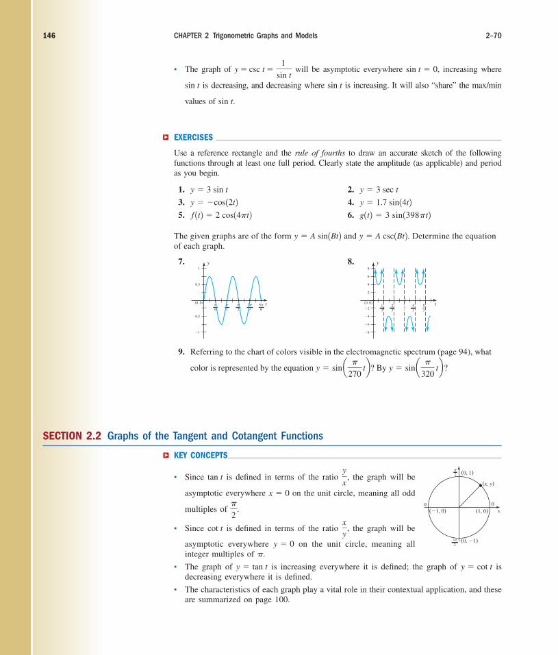
146
SECTION 2.2 Graphs of the Tangent and Cotangent Functions
KEY CONCEPTS
• Since is defined in terms of the ratio , the graph will be
asymptotic everywhere on the unit circle, meaning all odd
multiples of .
• Since is defined in terms of the ratio , the graph will be
asymptotic everywhere on the unit circle, meaning allinteger multiples of
• The graph of is increasing everywhere it is defined; the graph of isdecreasing everywhere it is defined.
• The characteristics of each graph play a vital role in their contextual application, and theseare summarized on page 100.
y � cot ty � tan t
�.y � 0
xy
cot t
�
2
x � 0
y
xtan t
▼
• The graph of will be asymptotic everywhere increasing where
is decreasing, and decreasing where is increasing. It will also “share” the max/min
values of
EXERCISES
Use a reference rectangle and the rule of fourths to draw an accurate sketch of the followingfunctions through at least one full period. Clearly state the amplitude (as applicable) and periodas you begin.
sin t.
sin tsin t
sin t � 0,y � csc t �1
sin t
▼
1.
3.
5.
2.
4.
6. g1t2 � 3 sin 1398�t2y � 1.7 sin14t2y � 3 sec t
f 1t2 � 2 cos14�t2y � �cos12t2y � 3 sin t
The given graphs are of the form and Determine the equationof each graph.
y � A csc1Bt2.y � A sin1Bt27. 8.
(0, 0)13
23
43
53
y
�2
�4
�6
�8
6
8
2
4
t11
(0, 0)�
6�
3�
22�
35�
6
y
�0.5
�1
1
0.5
t
9. Referring to the chart of colors visible in the electromagnetic spectrum (page 94), what
color is represented by the equation ? By ? y � sin a �
320 tby � sin a �
270 tb
CHAPTER 2 Trigonometric Graphs and Models 2–70
x0
(x, y)
(1, 0)
(0, 1)
(0, �1)
(�1, 0)
3�
2
�
2
�
cob10054_ch02_77-158.qxd 10/17/06 9:39 PM Page 146CONFIRMING PAGES
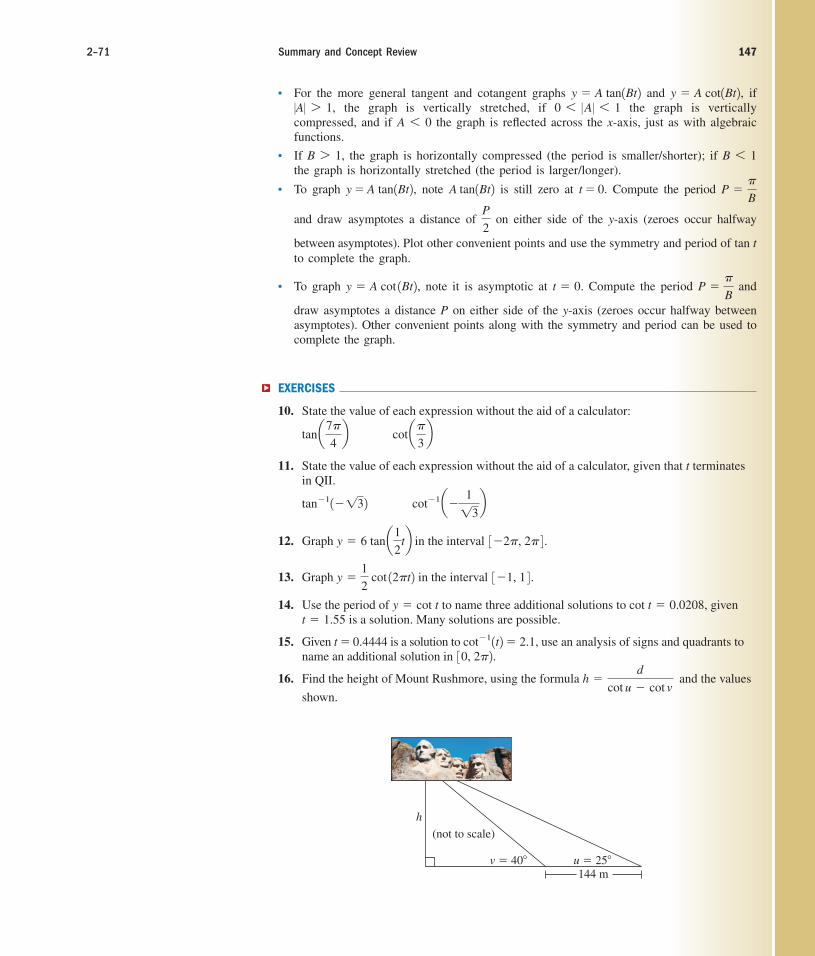
147
▼
2–71 Summary and Concept Review
• For the more general tangent and cotangent graphs and ifthe graph is vertically stretched, if the graph is vertically
compressed, and if the graph is reflected across the x-axis, just as with algebraicfunctions.
• If the graph is horizontally compressed (the period is smaller/shorter); if the graph is horizontally stretched (the period is larger/longer).
• To graph note is still zero at Compute the period
and draw asymptotes a distance of on either side of the y-axis (zeroes occur halfway
between asymptotes). Plot other convenient points and use the symmetry and period of to complete the graph.
• To graph note it is asymptotic at Compute the period and
draw asymptotes a distance P on either side of the y-axis (zeroes occur halfway betweenasymptotes). Other convenient points along with the symmetry and period can be used tocomplete the graph.
EXERCISES
10. State the value of each expression without the aid of a calculator:
11. State the value of each expression without the aid of a calculator, given that t terminatesin QII.
12. Graph in the interval .
13. Graph in the interval
14. Use the period of to name three additional solutions to givenis a solution. Many solutions are possible.
15. Given is a solution to use an analysis of signs and quadrants toname an additional solution in
16. Find the height of Mount Rushmore, using the formula and the values
shown.
h �d
cot u � cot v
30, 2�2.cot�11t2� 2.1,t � 0.4444
t � 1.55cot t � 0.0208,y � cot t
3�1, 1 4 .y �1
2 cot 12�t2
3�2�, 2� 4y � 6 tan a1
2tb
cot�1 a� 113
btan�11�132
cot a�
3btan a7�
4b
P ��
Bt � 0.y � A cot 1Bt2,
tan t
P
2
P ��
Bt � 0.A tan1Bt2y � A tan1Bt2,
B 6 1B 7 1,
A 6 00 6 �A� 6 1�A� 7 1,
y � A cot1Bt2,y � A tan1Bt2
(not to scale)
h
v � 40�144 m
u � 25�
cob10054_ch02_77-158.qxd 12/10/06 16:43 Page 147 CONFIRMING PAGES
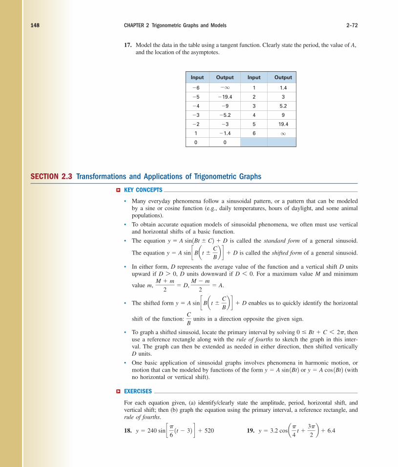
148
SECTION 2.3 Transformations and Applications of Trigonometric Graphs
KEY CONCEPTS
• Many everyday phenomena follow a sinusoidal pattern, or a pattern that can be modeledby a sine or cosine function (e.g., daily temperatures, hours of daylight, and some animalpopulations).
• To obtain accurate equation models of sinusoidal phenomena, we often must use verticaland horizontal shifts of a basic function.
• The equation is called the standard form of a general sinusoid.
The equation is called the shifted form of a general sinusoid.
• In either form, D represents the average value of the function and a vertical shift D unitsupward if D units downward if For a maximum value M and minimum
value m,
• The shifted form enables us to quickly identify the horizontal
shift of the function: units in a direction opposite the given sign.
• To graph a shifted sinusoid, locate the primary interval by solving thenuse a reference rectangle along with the rule of fourths to sketch the graph in this inter-val. The graph can then be extended as needed in either direction, then shifted verticallyD units.
• One basic application of sinusoidal graphs involves phenomena in harmonic motion, ormotion that can be modeled by functions of the form or (withno horizontal or vertical shift).
EXERCISES
For each equation given, (a) identify/clearly state the amplitude, period, horizontal shift, andvertical shift; then (b) graph the equation using the primary interval, a reference rectangle, andrule of fourths.
y � A cos 1Bt2y � A sin 1Bt2
0 � Bt � C 6 2�,
C
B
y � A sin cB at �C
Bb d � D
M � m
2� D,
M � m
2� A.
D 6 0.D 7 0,
y � A sin cB at �C
Bb d � D
y � A sin 1Bt � C2 � D
▼▼
18. 19. y � 3.2 cos a�
4 t �
3�
2b � 6.4y � 240 sin c�
6 1t � 32 d � 520
CHAPTER 2 Trigonometric Graphs and Models 2–72
17. Model the data in the table using a tangent function. Clearly state the period, the value of A,and the location of the asymptotes.
Input Output Input Output
1 1.4
2 3
3 5.2
4 9
5 19.4
1 6
0 0
q�1.4
�3�2
�5.2�3
�9�4
�19.4�5
�q�6
cob10054_ch02_77-158.qxd 12/10/06 16:43 Page 148 CONFIRMING PAGES

149
Day Dayof Year Output of Year Output
1 4430 184 90
31 3480 214 320
62 3050 245 930
92 1890 275 2490
123 1070 306 4200
153 790 336 4450
SECTION 2.4 Trigonometric Models
KEY CONCEPTS
• If the period P and critical points (X, M) and (x, m) of a sinusoidal function are known,a model of the form can be obtained:
• If an event or phenomenon is known to be sinusoidal, a graphing calculator can be usedto find an equation model if at least four data points are given.
EXERCISES
For the following sets of data, (a) find a sinusoidal regression equation using your calcula-tor; (b) construct an equation manually using the period and maximum/minimum values;and (c) graph both on the same screen, then use a TABLE to find the largest differencebetween output values.
23. 24.
C �3�
2� BxD �
M � m
2A �
M � m
2B �
2�
P
y � A sin1Bx � C2 � D
▼▼
2–73 Summary and Concept Review
25. The record high temperature for the even months of the year are given in the table forthe city of Juneau, Alaska. (a) Use a graphing calculator to find a sinusoidal regression
20. 21.
30
0
60
90
120
150
180
210
�
4�
23�
4�
t
y
t60
12 18 24
50
100
150
200
250
300
350
y
22. Monthly precipitation in Cheyenne, Wyoming, can be modeled by a sine function, by us-ing the average precipitation for July (2.26 in.) as a maximum (actually slightly higher inMay), and the average precipitation for February (0.44 in.) as a minimum. Assume t � 0corresponds to March. (a) Use the information to construct a sinusoidal model, and (b)use the model to estimate the inches of precipitation Cheyenne receives in August (t � 5)and December (t � 9).
Source: 2004 Statistical Abstract of the United States, Table 380.
For each graph given, identify the amplitude, period, horizontal shift, and vertical shift, andgive the equation of the graph.
Day Dayof Month Output of Month Output
1 69 19 98
4 78 22 92
7 84 25 85
10 91 28 76
13 96 31 67
16 100
cob10054_ch02_77-158.qxd 12/10/06 16:43 Page 149 CONFIRMING PAGES
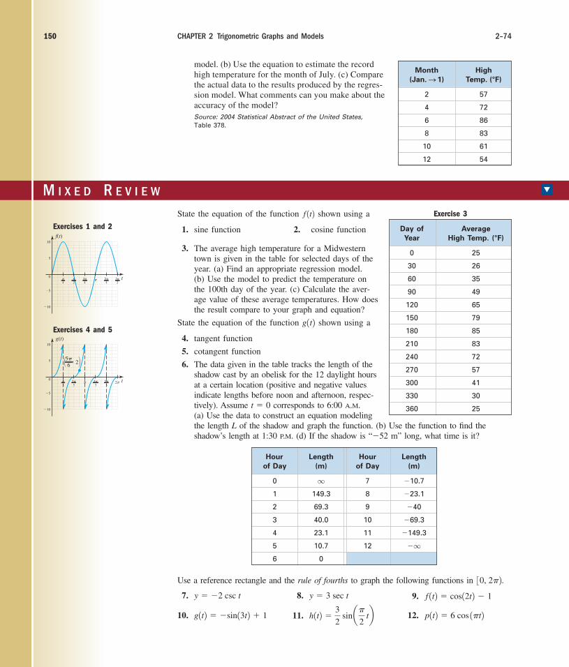
150 CHAPTER 2 Trigonometric Graphs and Models 2–74
Hour Length Hour Lengthof Day (m) of Day (m)
0 7 �10.7
1 149.3 8 �23.1
2 69.3 9 �40
3 40.0 10 �69.3
4 23.1 11 �149.3
5 10.7 12 �
6 0
q
q
M I X E D R E V I E W ▼
State the equation of the function shown using a
1. sine function 2. cosine function
3. The average high temperature for a Midwesterntown is given in the table for selected days of theyear. (a) Find an appropriate regression model.(b) Use the model to predict the temperature onthe 100th day of the year. (c) Calculate the aver-age value of these average temperatures. How doesthe result compare to your graph and equation?
State the equation of the function shown using a
4. tangent function
5. cotangent function
6. The data given in the table tracks the length of theshadow cast by an obelisk for the 12 daylight hoursat a certain location (positive and negative valuesindicate lengths before noon and afternoon, respec-tively). Assume corresponds to 6:00 A.M.(a) Use the data to construct an equation modelingthe length L of the shadow and graph the function. (b) Use the function to find theshadow’s length at 1:30 P.M. (d) If the shadow is “�52 m” long, what time is it?
t � 0
g1t2
f 1t2
�10
�5
0
10
5
t
f(t)
�4
3�4
5�4
3�2
��2
Exercises 1 and 2
�10
�5
0
10
5
t
g(t)
�3
4�3
5�3
� 2�2�3
5�6� , 2�
Exercises 4 and 5
Exercise 3
model. (b) Use the equation to estimate the recordhigh temperature for the month of July. (c) Comparethe actual data to the results produced by the regres-sion model. What comments can you make about theaccuracy of the model?Source: 2004 Statistical Abstract of the United States,
Table 378.
Month High(Jan. 1) Temp. (°F)
2 57
4 72
6 86
8 83
10 61
12 54
S
Day of AverageYear High Temp. (°F)
0 25
30 26
60 35
90 49
120 65
150 79
180 85
210 83
240 72
270 57
300 41
330 30
360 25
7. 8. 9. f 1t2 � cos12t2 � 1y � 3 sec ty � �2 csc t
Use a reference rectangle and the rule of fourths to graph the following functions in .30, 2�2
10. 11. 12. p1t2 � 6 cos 1�t2h1t2 �3
2 sin a�
2 tbg1t2 � �sin13t2 � 1
cob10054_ch02_77-158.qxd 12/10/06 16:43 Page 150 CONFIRMING PAGES

1511512–75 Practice Test
P R A C T I C E T E S T ▼
1. Complete the table using exact values, including the point on the unit circle associatedwith t.
13. Monthly precipitation in Minneapolis, Minnesota, can be modeled by a sine function,by using the average precipitation for August (4.05 in.) as a maximum (actuallyslightly higher in June), and the average precipitation for February (0.79 in.) as aminimum. Assume t � 0 corresponds to April. (a) Use the information to construct asinusoidal model, and (b) use the model to approximate the inches of precipitationMinneapolis receives in July (t � 3) and December (t � 8).
Source: 2004 Statistical Abstract of the United States, Table 380.
14. Which of the following functions indicates that the graph of has been shifted
horizontally units left?
a. b.
c. d.
15. Given is an approximate solution to , use an analysis of signsand quadrants to name another solution in
16. Solve each equation in [0, 2�) without the use of a calculator. If the expression isundefined, so state.
a. x � b. c.
d. e. f.
State the amplitude, period, horizontal shift, vertical shift, and endpoints of the primaryinterval, then sketch the graph using a reference rectangle and the rule of fourths.
17. 18.
State the period and phase shift, then sketch the graph of each function.
19. 20. y � 3 sec ax ��
2by � 2 tan a1
4 tb
y �7
2 sin c�
2 1x � 12 dy � 5 cos 12t2 � 8
tan a�
2b � xcsc x �
213
3cos � � x
cot a�
2b � xsec x � 12sin a��
4b
30, 2�2.tan t � �0.3t � 2.85
y � sin12t2 ��
4y � sin c2 at �
�
4b d
y � sin a2t ��
4by � sin c2 at �
�
4b d
�
4
y � sin12t2
t 0
sin t
cos t
tan t
csc t
sec t
cot t
P (x, y)
3�
24�
35�
45�
62�
3�
2�
4�
6
cob10054_ch02_77-158.qxd 12/10/06 16:43 Page 151 CONFIRMING PAGES

152152 CHAPTER 2 Trigonometric Graphs and Models 2–76
2. State the value of each expression without the use of a calculator:
a. b. c. d.
3. State the value of each expression without the use of a calculator:
a. b.
c. d.
State the amplitude (if it exists) and period of each function, then sketch the graph in theinterval indicated using a reference rectangle and the rule of fourths.
4. 5. ,
6. ,
State the amplitude (if it exists), period, horizontal shift, and vertical shift of each function,then sketch the graph in the interval indicated using a reference rectangle and the rule offourths.
7. 8.
9.
10. The revenue for Otake’s Mower Repair is very seasonal, with business in thesummer months far exceeding business in the winter months. Monthly revenue for the
company can be modeled by the function where
is the average revenue (in thousands of dollars) for month (a) What isthe average revenue for September? (b) For what months of the year is revenue atleast $12,500?
11. Given is a solution to use the period to find two othersolutions.
12. Given is a solution to , find another solution using a referenceangle/arc.
13. Although Reno, Nevada, is a very arid city, the amountof monthly precipitation tends to follow a sinusoidalpattern. (a) Find an equation model for the precipita-tion in Reno, given the annual high is 1.06 in., whileannual low is 0.24 in. and occurs in the month of July. (b) In what month does the annual high occur?
14. The lowest record temperature for the even monthsof the year are given in the table for the city ofDenver, Colorado. (a) Use a graphing calculator tofind a sinusoidal regression model, and (b) use theequation to estimate the record low temperature forthe odd numbered months.Source: 2004 Statistical Abstract of the United States, Table 379.
15. Due to tidal motions, the depth of water in Brentwood Bay varies sinusoidally asshown in the diagram, where time is in hours and depth is in feet. Find an equationthat models the depth of water at time t.
16. Determine the equation of the graph shown, given it is of the form y � A csc 1Bt2 � D.
tan�11t2 � 9t � 1.4602
P � �tan t � 2,t � 4.25
x 1x � 1 S Jan2.R 1x2R 1x2 � 7.5 cos a�
6 x �
4�
3b � 12.5,
y � 2 cot c 13
� at �3
2b d , t � 30, 62
y �3
4 cos a1
2 �tb �
1
2, t � 3�2, 62y � 12 sin c3at �
�
6b d � 19, t � 30, 2�2
t � 30, �2y � 4 tan 13t2t � 30, 2�2y � 2 sec 12t2t � 30, 102y � 3 sin a�
5 tb,
sec�1 1122; QIVsin�1 a�23
2b; QIII
cos�1 a�1
2b; QIItan�1
113 2; QI
sec a�
6btan a5�
4bsin � cos a3�
2b
Month High(Jan. 1) Temp. (°F)
2 �30
4 �2
6 30
8 41
10 3
12 �25
S
Exercise 14
Exercise 15
Time (hours)
Depth (ft)
20 241612840
8
4
16
20
12
Exercise 16
�4
�2
2
1 2 3 4 5 6 7 8
f(t)
t
cob10054_ch02_77-158.qxd 12/10/06 16:43 Page 152 CONFIRMING PAGES

2–77 Calculator Exploration and Discovery 153
▼C A L C U L A T O R E X P L O R A T I O N A N D D I S C O V E R Y
Variable Amplitudes andModeling the Tides
As mentioned in the Point of Interest from Section 2.3, tidal motion is often too complexto be modeled by a single sine function. In this Exploration and Discovery, we’ll look at amethod that combines two sine functions to help model a tidal motion with variable ampli-tude. In the process, we’ll use much of what we know about the amplitude, horizontal shifts,and vertical shifts of a sine function. The graph in Figure 2.46 shows three days of tidalmotion for Davis Inlet, Canada.
0.90.7 0.8 0.7 0.7 0.6
2.42.4
2.01.9 1.92.3
t
Height (m)
0
1
2
Midnight Noon Midnight Noon Midnight Noon Midnight
As you can see, the amplitude of the graph varies, and there is no single sine function thatcan serve as a model. However, notice that the amplitude varies predictably, and that the hightides and low tides can independently be modeled by a sine function. To simplify our explo-ration, we will use the assumption that tides have an exact 24-hr period (close, but no), thatvariations between high and low tides takes place every 12 hr (again close but not exactly true),
Figure 2.46
Match each equation with its corresponding graph.
17. 18.
19. 20.
a. b.
c. d.
y � 3 sin a2t ��
6by � �3 sin 1�t2 � 1
y � 3 sin 1�t2 � 1y � 3 sin c2 at ��
6b d
2�
�2
�1
�4
�3
2
1
3
4
�
y
t 61 2 3 4 5
�2
�1
�4
�3
2
1
3
4
y
t
61 2 3 4 5
�2
�1
�4
�3
2
1
3
4
y
t
�2
�1
�4
�3
2
1
3
4
y
t2���
23�
2
cob10054_ch02_77-158.qxd 12/10/06 16:43 Page 153 CONFIRMING PAGES
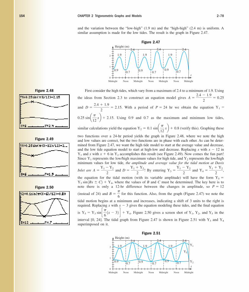
CHAPTER 2 Trigonometric Graphs and Models 2–78154
Figure 2.51
0.90.7 0.9 0.7 0.7
2.42.4
1.91.9 1.9
Y2
Y5
Y1
2.4
t
Height (m)
0
1
2
Midnight Noon Midnight Noon Midnight Noon Midnight
0.9
Figure 2.50
0.90.7 0.9 0.7
0.90.7
2.42.4
1.91.9 1.9
2.4
t
Height (m)
0
1
2
Midnight Noon Midnight Noon Midnight Noon Midnight
Figure 2.47
First consider the high tides, which vary from a maximum of 2.4 to a minimum of 1.9. Using
the ideas from Section 2.3 to construct an equation model gives
and With a period of hr we obtain the equation
Using 0.9 and 0.7 as the maximum and minimum low tides,
similar calculations yield the equation (verify this). Graphing these
two functions over a 24-hr period yields the graph in Figure 2.48, where we note the highand low values are correct, but the two functions are in phase with each other. As can be deter-mined from Figure 2.47, we want the high tide model to start at the average value and decrease,and the low tide equation model to start at high-low and decrease. Replacing x with in
and x with in accomplishes this result (see Figure 2.49). Now comes the fun part!Since represents the low/high maximum values for high tide, and represents the low/highminimum values for low tide, the amplitude and average value for the tidal motion at Davis
Inlet are and By entering and
the equation for the tidal motion (with its variable amplitude) will have the form where the values of B and C must be determined. The key here is to
note there is only a 12-hr difference between the changes in amplitude, so
(instead of 24) and for this function. Also, from the graph (Figure 2.47) we note the
tidal motion begins at a minimum and increases, indicating a shift of 3 units to the right isrequired. Replacing x with gives the equation modeling these tides, and the final equation
is Figure 2.50 gives a screen shot of Y1, Y2, and Y5 in the
interval [0, 24]. The tidal graph from Figure 2.47 is shown in Figure 2.51 with and superimposed on it.
Y4Y3
Y3 sin c�6
1x � 32 d � Y4.Y5 �
x � 3
B ��
6
P � 12Y3 sin 1Bx � C2 � Y4,
Y5 �
Y4 �Y1 � Y2
2,Y3 �
Y1 � Y2
2D �
Y1 � Y2
2!A �
Y1 � Y2
2
Y2Y1
Y2x � 6Y1
x � 12
Y2 � 0.1 sin a �
12 xb � 0.8
2.15.0.25 sin a �
12 xb �
Y1 �P � 24D �2.4 � 1.9
2� 2.15.
A �2.4 � 1.9
2� 0.25
Figure 2.49
Figure 2.48
and the variation between the “low-high” (1.9 m) and the “high-high” (2.4 m) is uniform. Asimilar assumption is made for the low tides. The result is the graph in Figure 2.47.
cob10054_ch02_77-158.qxd 12/10/06 16:43 Page 154 CONFIRMING PAGES

2–79 Strengthening Core Skills 155
▼
Exercise 1: The website www.tides.com/tcpred.htm offers both tide and current predictionsfor various locations around the world, in both numeric and graphical form. Inaddition, data for the “two” high tides and “two” low tides are clearly highlighted.Select a coastal area where tidal motion is similar to that of Davis Inlet, andrepeat this exercise. Compare your model to the actual data given on the web-site. How good was the fit?
S T R E N G T H E N I N G C O R E S K I L L S
Standard Angles, ReferenceAngles, and the TrigFunctions
A review of the main ideas discussed in this chapter indicates there are four of what mightbe called “core skills.” These are skills that (a) play a fundamental part in the acquisition ofconcepts, (b) hold the overall structure together as we move from concept to concept, and(c) are ones we return to again and again throughout our study. The first of these is (1) know-ing the standard angles and standard values.
The standard angles/values brought us to the trigonometry of any angle, forming astrong bridge to the second core skill: (2) using reference angles to determine the valueof the trig functions in each quadrant. For any angle where or
since the ratio is fixed but the sign depends on the quadrant of : [QI], [QII], [QIII], [QIV], and so on (see Figure 2.52).sin 330° � �1
2sin 210° � �12sin 150° � 1
2
sin 30° � 12�sin � � �1
2
sin � � 12�r � 30°,�
In turn, the reference angles led us to a third core skill, helping us realize that if was not
a quadrantal angle, (3) equations like must have two solutions in
The solutions in are and (see Figure 2.53).Of necessity, this brings us to the fourth core skill, (4) effective use of a calculator.
The standard angles are a wonderful vehicle for introducing the basic ideas of trigonom-etry, and actually occur quite frequently in real-world applications. But by far, most ofthe values we encounter will be nonstandard values where must be found using acalculator.
The Summary and Concept Review Exercises, as well as the Practice Test offer ampleopportunities to refine these skills.
�r
� � 210°� � 150°30, 360°230, 360°2.cos 1�2 � �
13
2
�
2�2
�2
2
x
y
(�√3, �1)
(�√3, 1)
cos �r � 2√3
2
2
150�
210�
�r � 30�
�r � 30�
Figure 2.53Figure 2.52
2�2
�2
2
x
y
(�√3, �1)
(�√3, 1)
(√3, �1)
(√3, 1)
sin �r � 21
2
2
2
2
�r � 30�
�r � 30�
�r � 30�
�r � 30�
cob10054_ch02_77-158.qxd 12/10/06 16:44 Page 155 CONFIRMING PAGES

6. During a storm, a tall tree snapped, as shown in thediagram. Find the tree’s original height. Round to tenthsof a meter.
7. Find the measure of angle � for the triangle shown andconvert it to
a. decimal degrees b. radians
CHAPTER 2 Trigonometric Graphs and Models 2–80156
▼C U M U L A T I V E R E V I E W C H A P T E R S 1 – 2
1. Use a reference rectangle and the rule of fourths to graph in .
2. State the period, horizontal shift, and x-intercepts of the function
in Then state whether the function is increasing or decreasing and sketch its
graph.
3. Given that draw a right triangle that corresponds to this ratio, then use the
Pythagorean theorem to find the length of the missing side. Finally, find the two acute angles.
tan � �80
39,
c��
2, �b.
y � �tan a2x ��
2b
3�2, 62y � 2.5 sin a�
2 tb
4. Without a calculator, what values inmake the equation true:
?sin t � �13
2
30, 2�2 5. Given is a point on the unit
circle corresponding to t, find all sixtrig functions of t.
a3
4, �17
4b
12 cm
56�
t 0
tan t �y
x
cos t � x
sin t � y
5�
47�
6�
5�
63�
42�
3�
2�
3�
4�
6
Exercise 1: Fill in the table from memory.
Exercise 2: Solve each equation in without the use of a calculator.
a. b.
c. d.
Exercise 3: Solve each equation in using a calculator and rounding answers to fourdecimal places.
a. b.
c. d. 2 sec t � �53 tan t �1
2� �
1
4
�312 cos t � 12 � 016 sin t � 2 � 1
30, 2�2
2 sin t � 1�13 tan t � 2 � 1
� 312 cos t � 4 � 12 sin t � 13 � 0
30, 2�2
Exercise 6
Exercise 7
29� 24'54"
�
cob10054_ch02_145-158.qxd 11/22/06 9:39 AM Page 156
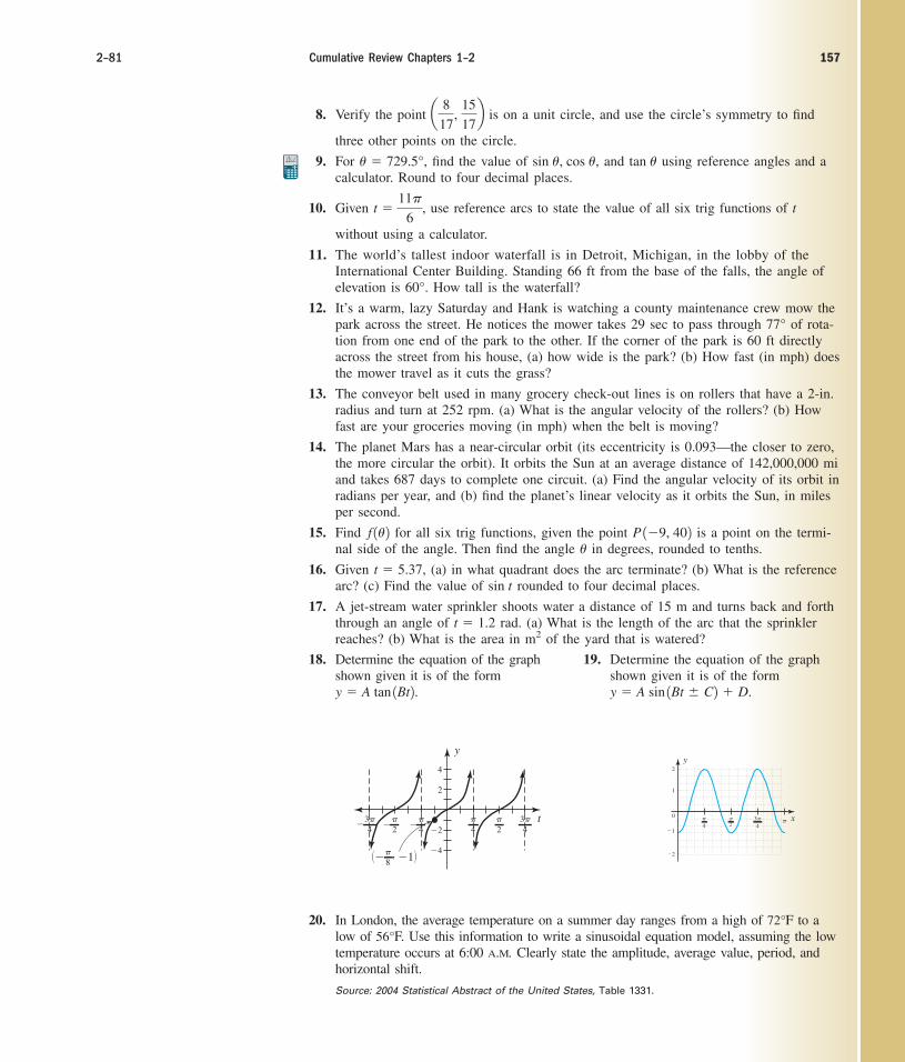
2–81 Cumulative Review Chapters 1–2 157
y
t3�4
3�4
�4
�2
�4
�4
�2
4
2
��2��
�8�� , �1� �2
�1
0
1
2
y
x�
4� 3�
4�
2
18. Determine the equation of the graphshown given it is of the form
19. Determine the equation of the graphshown given it is of the formy � A sin 1Bt � C2 � D.y � A tan 1Bt2.
20. In London, the average temperature on a summer day ranges from a high of F to alow of F. Use this information to write a sinusoidal equation model, assuming the lowtemperature occurs at 6:00 A.M. Clearly state the amplitude, average value, period, andhorizontal shift.
Source: 2004 Statistical Abstract of the United States, Table 1331.
56°72°
8. Verify the point is on a unit circle, and use the circle’s symmetry to find
three other points on the circle.
9. For , find the value of and using reference angles and acalculator. Round to four decimal places.
10. Given use reference arcs to state the value of all six trig functions of t
without using a calculator.
11. The world’s tallest indoor waterfall is in Detroit, Michigan, in the lobby of theInternational Center Building. Standing 66 ft from the base of the falls, the angle ofelevation is How tall is the waterfall?
12. It’s a warm, lazy Saturday and Hank is watching a county maintenance crew mow the park across the street. He notices the mower takes 29 sec to pass through of rota-tion from one end of the park to the other. If the corner of the park is 60 ft directlyacross the street from his house, (a) how wide is the park? (b) How fast (in mph) doesthe mower travel as it cuts the grass?
13. The conveyor belt used in many grocery check-out lines is on rollers that have a 2-in.radius and turn at 252 rpm. (a) What is the angular velocity of the rollers? (b) Howfast are your groceries moving (in mph) when the belt is moving?
14. The planet Mars has a near-circular orbit (its eccentricity is 0.093—the closer to zero,the more circular the orbit). It orbits the Sun at an average distance of 142,000,000 miand takes 687 days to complete one circuit. (a) Find the angular velocity of its orbit inradians per year, and (b) find the planet’s linear velocity as it orbits the Sun, in milesper second.
15. Find for all six trig functions, given the point is a point on the termi-nal side of the angle. Then find the angle in degrees, rounded to tenths.
16. Given (a) in what quadrant does the arc terminate? (b) What is the referencearc? (c) Find the value of rounded to four decimal places.
17. A jet-stream water sprinkler shoots water a distance of 15 m and turns back and forththrough an angle of rad. (a) What is the length of the arc that the sprinklerreaches? (b) What is the area in of the yard that is watered?m2
t � 1.2
sin tt � 5.37,
�P 1�9, 402f 1�2
77°
60°.
t �11�
6,
tan �sin �, cos �,� � 729.5°
a 8
17,
15
17b
cob10054_ch02_77-158.qxd 10/17/06 2:12 PM Page 157CONFIRMING PAGES

21. State true or false and explain your response:
22. Complete the following statement: The cofunction of sine is cosine because . . . .
23. Find the value of all six trig functions given and
24. The profits of Red-Bud Nursery can be modeled by a sinusoid, with profit peakingtwice each year. Given profits reach a yearly low of $4000 in mid-January (month 1.5),and a yearly high of $14,000 in mid-April (month 4.5), (a) construct an equation fortheir yearly profits. (b) Use the model to find their profits for August. (c) Name theother month at which profit peaks.
25. The Earth has a radius of 3960 mi. Mexico City, Mexico, is located at approximatelyN latitude, and is almost exactly due south of Hutchinson, Kansas, located at
about N latitude. How many miles separate the two cities?38°19°
sin t 7 0.tan t � �68
51
1sin t2 1sec t2 � 1.
CHAPTER 2 Trigonometric Graphs and Models 2–82158
cob10054_ch02_77-158.qxd 12/10/06 16:44 Page 158 CONFIRMING PAGES